generalized linear mixed models (illustrated with r on ... · generalized linear mixed ......
TRANSCRIPT

Generalized Linear Mixed Models
(illustrated with R on Bresnan et al.’s datives data)
Christopher Manning
23 November 2007
In this handout, I present the logistic model with fixed and random effects, a form of Generalized LinearMixed Model (GLMM). I illustrate this with an analysis of Bresnan et al. (2005)’s dative data (the versionsupplied with the languageR library). I deliberately attempt this as an independent analysis. It is animportant test to see to what extent two independent analysts will come up with the same analysis of a setof data. Sometimes the data speaks so clearly that anyone sensible would arrive at the same analysis. Often,that is not the case. It also presents an opportunity to review some exploratory data analysis techniques, aswe start with a new data set. Often a lot of the difficulty comes in how to approach a data set and to definea model over which variables, perhaps transformed.
1 Motivating GLMMs
I briefly summarize the motivations for GLMMs (in linguistic modeling):
• The Language-as-fixed-effect-fallacy (Clark 1973 following Coleman 1964). If you want to make state-ments about a population but you are presenting a study of a fixed sample of items, then you cannotlegitimately treat the items as a fixed effect (regardless of whether the identity of the item is a factorin the model or not) unless they are the whole population.
– Extension: Your sample of items should be a random sample from the population about whichclaims are to be made. (Often, in practice, there are sampling biases, as Bresnan has discussedfor linguistics in some of her recent work. This can invalidate any results.)
• Ignoring the random effect (as is traditional in psycholinguistics) is wrong. Because the often significantcorrelation between data coming from one speaker or experimental item is not modeled, the standarderror estimates, and hence significances are invalid. Any conclusion may only be true of your randomsample of items, and not of another random sample.
• Modeling random effects as fixed effects is not only conceptually wrong, but often makes it impossibleto derive conclusions about fixed effects because (without regularization) unlimited variation can beattributed to a subject or item. Modeling these variables as random effects effectively limits how muchvariation is attributed to them (there is an assumed normal distribution on random effects).
• For categorical response variables in experimental situations with random effects, you would like tohave the best of both worlds: the random effects modeling of ANOVA and the appropriate modelingof categorical response variables that you get from logistic regression. GLMMs let you have bothsimultaneously (Jaeger 2007). More specifically:
– A plain ANOVA is inappropriate with a categorical response variable. The model assumptionsare violated (variance is heteroscedastic, whereas ANOVA assumes homoscedasticity). This leadsto invalid results (spurious null results and significances).
1

– An ANOVA can perform poorly even if transformations of the response are performed. At anyrate, there is no reason to use this technique: cheap computing makes use of a transformedANOVA unnecessary.
– A GLMM gives you all the advantages of a logistic regression model:1
∗ Handles a multinomial response variable.
∗ Handles unbalanced data
∗ Gives more information on the size and direction of effects
∗ Has an explicit model structure, adaptable post hoc for different analyses (rather than re-quiring different experimental designs)
∗ Can do just one combined analysis with all random effects in it at once.
• Technical statistical advantages (Baayen, Davidson, and Bates). Maybe mainly incomprehensible, butyou can trust that worthy people think the enterprise worthy.
– Traditional methods have deficiencies in power (you fail to demonstrate a result that you shouldbe able to demonstrate)
– GLMMs can robustly handle missing data, while traditional methods cannot.
– ?? GLMMs improve on disparate methods for treating continuous and categorical responses ??.[I never quite figured out what this one meant – maybe that working out ANOVA models andtractable approximations for different cases is tricky, difficult stuff?]
– You can avoid unprincipled methods of modeling heteroscedasticity and non-spherical error vari-ance.
– It is practical to use crossed rather than nested random effects designs, which are usually moreappropriate
– You can actually empirically test whether a model requires random effects or not.
∗ But in practice the answer is usually yes, so the traditional ANOVA practice of assuming yesis not really wrong.
– GLMMs are parsimonious in using parameters, allowing you to keep degrees of freedom (givingsome of the good effects listed above). The model only estimates a variance for each randomeffect.
2 Exploratory Data Analysis (EDA)
First load the data (I assume you have installed the languageR package already). We will use the dativedata set, which we load with the data function. Typing dative at the command line would dump it to yourwindow, but that isn’t very useful for large data sets. You can instead get a summary:
> library(languageR)
> data(dative)
> summary(dative)
Speaker Modality Verb SemanticClass LengthOfRecipient AnimacyOfRec
S1104 : 40 spoken :2360 give :1666 a:1433 Min. : 1.000 animate :3024
S1083 : 30 written: 903 pay : 207 c: 405 1st Qu.: 1.000 inanimate: 239
S1151 : 30 sell : 206 f: 59 Median : 1.000
S1139 : 29 send : 172 p: 228 Mean : 1.842
1Jaeger’s suggesting that GLMMs give you the advantage of penalized likelihood models is specious; similar regularizationmethods have been developed and are now widely used for every type of regression analysis, and ANOVA is equivalent to atype of linear regression analysis, as Jaeger notes.
2
S1019 : 28 cost : 169 t:1138 3rd Qu.: 2.000
(Other):2203 tell : 128 Max. :31.000
NA’s : 903 (Other): 715
DefinOfRec PronomOfRec LengthOfTheme AnimacyOfTheme DefinOfTheme
definite :2775 nonpronominal:1229 Min. : 1.000 animate : 74 definite : 929
indefinite: 488 pronominal :2034 1st Qu.: 2.000 inanimate:3189 indefinite:2334
Median : 3.000
Mean : 4.272
3rd Qu.: 5.000
Max. :46.000
PronomOfTheme RealizationOfRecipient AccessOfRec AccessOfTheme
nonpronominal:2842 NP:2414 accessible: 615 accessible:1742
pronominal : 421 PP: 849 given :2302 given : 502
new : 346 new :1019
Much more useful!In terms of the discussion in the logistic regresssion handout, this is long form data – each observed data
point is a row. Though note that in a case like this with many explanatory variables, the data wouldn’tactually get shorter if presented as summary statistics, because the number of potential cells (# speakers ×# Modality × # Verb × . . . ) well exceeds the observed number of data items. The data has also all beenset up right, with categorical variables made into factors etc. If you are starting from data read in from atab-separated text file, that’s often the first thing to do.
If you’ve created a data set, you might know it intimately. Otherwise, it’s always a good idea to get agood intuitive understanding of what is there. The response variable is RealizationOfRecipient (long variablenames, here!). Note the very worrying fact that over half the tokens in the data are instances of the verbgive. If it’s behavior is atypical relative to ditransitive verbs, that will skew everything. Under, Speaker,NA is R’s special “not available” value for missing data. Unavailable data attributes are very common inpractice, but often introduce extra statistical issues (and you often have to be careful to check how R ishandling the missing values). Here, we guess from the matching 903’s that all the written data doesn’t havethe Speaker listed. Since we’re interested in a mixed effects model with Speaker as a random effect, we’llwork with just the spoken portion (which is the Switchboard data).
spdative <- subset(dative, Modality=="spoken")
You should look at the summary again, and see how it has changed. It has changed a bit (almost all thepronominal recipients are in the spoken data, while most of the nonpronominal recipients are in the writtendata; nearly all the animate themes are in the spoken data). It’s also good just to look at a few rows (notethat you need that final comma in the array selector!):
> spdative[1:5,]
Speaker Modality Verb SemanticClass LengthOfRecipient AnimacyOfRec DefinOfRec
903 S1176 spoken give a 1 inanimate definite
904 S1110 spoken give c 2 animate indefinite
905 S1110 spoken pay a 1 animate definite
906 S1146 spoken give a 2 animate definite
907 S1146 spoken give t 2 animate definite
PronomOfRec LengthOfTheme AnimacyOfTheme DefinOfTheme PronomOfTheme
903 pronominal 2 inanimate indefinite nonpronominal
904 nonpronominal 1 inanimate definite pronominal
905 pronominal 1 inanimate indefinite nonpronominal
906 nonpronominal 4 inanimate indefinite nonpronominal
907 nonpronominal 3 inanimate definite nonpronominal
3
spdative.xtabs
RealizationOfRecipient
Ani
mac
yOfR
ec
NP PP
anim
ate
inan
imat
e
animate inanimate animate inanimate
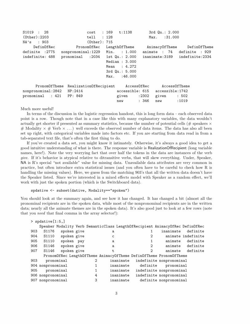
Figure 1: Mosaic plot. Most data instances are animate recipient, inanimate theme, realized as an NPrecipient.
RealizationOfRecipient AccessOfRec AccessOfTheme
903 NP given accessible
904 PP new given
905 PP given accessible
906 NP accessible new
907 PP accessible accessible
2.1 Categorical predictors
Doing exploratory data analysis of categorical variables is harder than for numeric variables. But it’s certainlyuseful to look at crosstabs (even though, as discussed, you should trust regression outputs not the marginalsof crosstabs for what factors are important). But they give you a sense of the data, and having done this willat least allow you to notice when you make a mistake in model building and the predictions of the modelproduced are clearly not right. For just a couple of variables, you can also graph them with a mosaicplot. Butthat quickly becomes unreadable for too many variables at once. . . . Figure 1 already isn’t that informativeto me beyond the crosstabs. I concluded that a majority of the data instances have inanimate theme andanimate recipient, and these are overwhelmingly realized as a ditransitive (NP recipient).
> spdative.xtabs <- xtabs(~ RealizationOfRecipient + AnimacyOfRec + AnimacyOfTheme)
> spdative.xtabs
, , AnimacyOfTheme = animate
AnimacyOfRec
RealizationOfRecipient animate inanimate
NP 17 0
PP 46 5
4
, , AnimacyOfTheme = inanimate
AnimacyOfRec
RealizationOfRecipient animate inanimate
NP 1761 81
PP 378 72
> mosaicplot(spdative.xtabs, color=T)
These methods should be continued looking at various of the other predictors in natural groups. The responseis very skewed: 1859/(1859 + 501) = 78.8% of the examples are NP realization (ditransitives). Looking atother predictors, most of the data is also indefinite theme and definite recipient, realized as an NP. Andmost of the data is nonpronominal theme and pronominal recipient which is overwhelmingly realized as anNP. With slightly less skew, much of the data has anaccessible theme and a given recipient, usually realizedas an NP. For semantic class, “t” stands out as preferring PP realization of the theme (see Bresnan et al.(2005, p. 12) on these semantic classes – “t” is transfer of possession). Class “p” (prevention of possession)really seems to prefer NP realization. Finally, we might check whether give does on average behave like otherverbs. The straight marginal looks okay (if probably not passing a test for independence). A crosstab alsoincluding PronomOfRec looks more worrying: slightly over half of instances of give with a nonpronominalrecipient NP are nevertheless ditransitive, whereas less than one third over such cases with other verbs haveNP realization. Of course, there may be other factors which explain this, which a regression analysis cantease out.
> xtabs(~ RealizationOfRecipient + I(Verb == "give"))
I(Verb == "give")
RealizationOfRecipient FALSE TRUE
NP 776 1083
PP 321 180
> xtabs(~ RealizationOfRecipient + I(Verb == "give") + PronomOfRec)
, , PronomOfRec = nonpronominal
I(Verb == "give")
RealizationOfRecipient FALSE TRUE
NP 83 109
PP 185 98
, , PronomOfRec = pronominal
I(Verb == "give")
RealizationOfRecipient FALSE TRUE
NP 693 974
PP 136 82
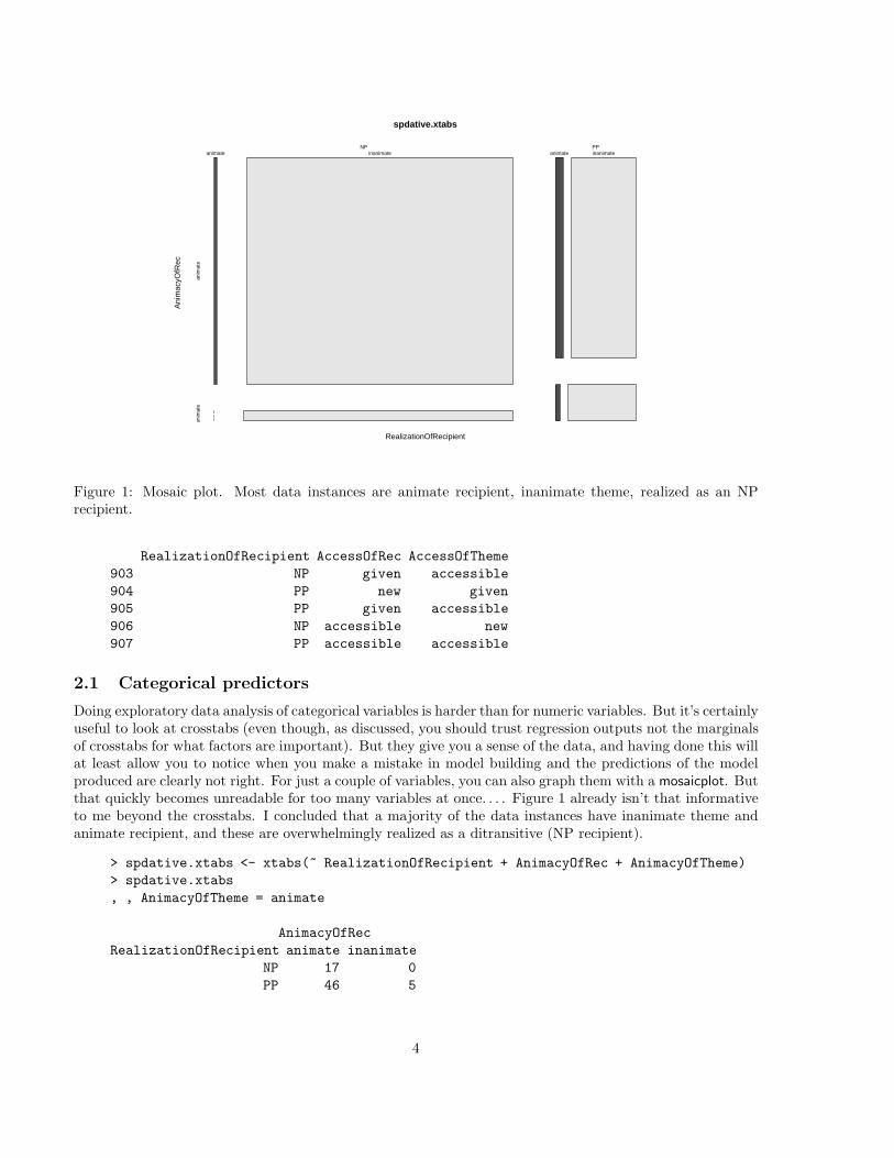
It can also be useful to do crosstabs without the response variable. An obvious question is how pronom-inality, definiteness, and animacy interrelate. I put a couple of mosaic plots for this in Figure 2. Theirdistribution is highly skewed and strongly correlated.2
2.2 Numerical predictors
There are some numeric variables (integers, not real numbers): the two lengths. If we remember the Wasowpaper and Hawkins’s work, we might immediately also wonder where the difference between these two
2These two were drawn with the mosaic() function in the vcd package, which has extra tools for visualizing categorical data.This clearly seems to have been what Baayen actually used to draw his Figure 2.6 (p. 36) and not mosaicplot(), despite whatis said on p. 35.
5
ThemeDefinOfTheme
An
imac
yOfT
hem
e
Pro
no
mO
fTh
eme
inan
imat
e
pron
omin
alno
npro
nom
inal
anim
ate definite indefinite
pron
omin
alno
npro
nom
inal
RecipientDefinOfRec
An
imac
yOfR
ec
Pro
no
mO
fRec
inan
imat
e
pron
omin
alno
npro
nom
inal
anim
ate
definite indefinite
pron
omin
alno
npro
nom
inal
Figure 2: Interaction of definiteness, animacy, and pronominality
lengths might be an even better predictor, so we’ll add it to the data frame. Thinking ahead to transformingexplanatory variables, it also seems useful to have the ratio of the two lengths. We’ll add these variablesbefore we attach to the data frame, so that they will be available.3
> spdative <- transform(spdative, LengthOfThemeMinusRecipient = LengthOfTheme - LengthOfRecipient)
> spdative <- transform(spdative, RatioOfLengthsThemeOverRecipient = LengthOfTheme / LengthOfRecipient)
> attach(spdative)
If we’re fitting a logistic model, we might check whether a logistic model works for these numeric variables.Does a unit change in length cause a constant change in the log odds. We could plot with untransformedvalues, looking for a logistic curve, but it is usually better to plot against logit values and to check againsta straight line. We’ll do both. First we examine the data with crosstabs:
> xtabs(~ RealizationOfRecipient + LengthOfRecipient)
LengthOfRecipient
RealizationOfRecipient 1 2 3 4 5 6 7 8 9 10 11 12 15
NP 1687 133 19 8 4 4 2 0 1 0 0 1 0
PP 228 139 61 24 12 8 9 8 2 4 2 3 1
> xtabs(~ RealizationOfRecipient + LengthOfTheme)
LengthOfTheme
RealizationOfRecipient 1 2 3 4 5 6 7 8 9 10 11 12 13 14 15 16
NP 358 515 297 193 145 77 75 46 35 22 20 19 12 9 13 1
PP 268 116 42 22 16 14 3 4 2 4 4 1 2 0 1 1
LengthOfTheme
RealizationOfRecipient 17 18 19 21 23 24 25 27 28 29 30 46
NP 3 3 5 2 1 2 1 1 1 1 1 1
PP 0 0 0 0 0 0 0 0 1 0 0 0
We could directly use length as an integer in our plot, but it gets hopelessly sparse for big lengths (P (NP realization) =0.33 for length 9 but 0 for length 8 or 10. . . ). So we will group using the cut command. This defines a factorby categoricalizing a numeric variable into ranges, but I’m going to preserve and use the numeric values inmy plot. I hand chose the cut divisions to put a reasonable amount of data into each bin. Given the integernature of most of the data, hand-done cuts seemed more sensible than cutting it automatically. (The output
3Of course, in reality, I didn’t do this. I only thought to add these variables later in the analysis. I then added them as here,and did an attach again. It complains about hiding the old variables, but all works fine.
6

of the cut command is a 2360 element vector mapping the lengths onto ranges. So I don’t print it out here!)The table command then produces a crosstab (like xtabs, but not using the model syntax), and prop.tablethen turns the counts into a proportion of a table by row, from which we take the first column (recipientNP realization proportion).
> divs <- c(0,1,2,3,4,5,6,10,100)
> divs2 <- c(-40,-6,-4,-3,-2,-1,0,1,2,3,4,6,40)
> divs3 <- c(-2.5,-1.5,-1,-0.5,-0.25,0,0.5,1,1.5,2,2.5,4)
> recip.leng.group <- cut(LengthOfRecipient, divs)
> theme.leng.group <- cut(LengthOfTheme, divs)
> theme.minus.recip.group <- cut(LengthOfThemeMinusRecipient, divs2)
> log.theme.over.recip.group <- cut(log(RatioOfLengthsThemeOverRecipient), divs3)
> recip.leng.table <- table(recip.leng.group, RealizationOfRecipient)
> recip.leng.table
RealizationOfRecipient
recip.leng.group NP PP
(0,1] 1687 228
(1,2] 133 139
(2,3] 19 61
(3,4] 8 24
(4,5] 4 12
(5,6] 4 8
(6,10] 3 23
(10,100] 1 6
> theme.leng.table <- table(theme.leng.group, RealizationOfRecipient)
> theme.minus.recip.table <- table(theme.minus.recip.group, RealizationOfRecipient)
> log.theme.over.recip.table <- table(log.theme.over.recip.group, RealizationOfRecipient)
> rel.freq.NP.recip.leng <- prop.table(recip.leng.table, 1)[,1]
> rel.freq.NP.recip.leng
(0,1] (1,2] (2,3] (3,4] (4,5] (5,6] (6,10] (10,100]
0.8809399 0.4889706 0.2375000 0.2500000 0.2500000 0.3333333 0.1153846 0.1428571
> rel.freq.NP.theme.leng <- prop.table(theme.leng.table, 1)[,1]
> rel.freq.NP.theme.minus.recip <- prop.table(theme.minus.recip.table, 1)[,1]
> rel.freq.NP.log.theme.over.recip <- prop.table(log.theme.over.recip.table, 1)[,1]
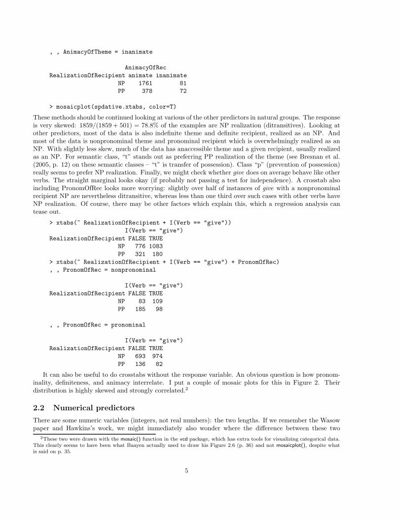
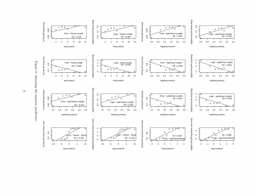
That’s a lot of setup! Doing EDA can be hard work. But now we can actually plot numeric predictorsagainst the response variable and fit linear models to see how well they correlate. It sticks out in the datathat most themes and recipients are quite short, but occasional ones can get very long. The data cries outfor some sort of data transform. sqrt() and log() are the two obvious data transforms that should come tomind when you want to transform data with this sort of distribution (with log() perhaps more natural here).We can try them out. We plot each of the raw and log and sqrt transformed values of each of theme andrecipient length against each of a raw probability of NP realization and the logit of that quantity, giving 12plots and 12 regressions. Then I make 4 more plots by considering the difference between their lengths andthe log of the ratio between their lengths against both the probability and the logit, giving 16 plots in total.Looking ahead to using a log() transform was why I defined the ratio of lengths – since I can’t apply log()to 0 or negative numbers, but it is completely sensible to apply it to a ratio. In fact, there is every reasonto think that this might be a good explanatory factor.
This gives a fairly voluminous amount of commands and output to wade through, so I will display thegraphical results in Figure 3, and put all the calculation details in an appendix. But you’ll need to look atthe calculation details to see what I did to produce the figure.
I made the regression lines by simply making linear models. I define a center for each factor, which is amixture of calculation and sometimes just a reasonable guess for the extreme values. Then I fit regressionlines by ordinary linear regression not logistic regression. So model fit is assessed by squared error (which
7
2 4 6 8 10 12
0.60
0.80
leng.centers
rel.f
req.
NP
.them
e.le
ng
Prob ~ Theme Length
R2 = 0.376
2 4 6 8 10 12
0.5
1.5
2.5
leng.centers
logi
t(re
l.fre
q.N
P.th
eme.
leng
)
Logit ~ Theme LengthR2 = 0.454
0.0 0.5 1.0 1.5 2.0 2.5
0.60
0.80
log(leng.centers)
rel.f
req.
NP
.them
e.le
ng
Prob ~ log(Theme Length)R2 = 0.684
0.0 0.5 1.0 1.5 2.0 2.5
0.5
1.5
2.5
log(leng.centers)
logi
t(re
l.fre
q.N
P.th
eme.
leng
)
Logit ~ log(Theme Length)R2 = 0.736
2 4 6 8 10 12
0.2
0.6
leng.centers
rel.f
req.
NP
.rec
ip.le
ng
Prob ~ Recip Length
R2 = 0.508
2 4 6 8 10 12
−2
01
2
leng.centers
logi
t(re
l.fre
q.N
P.r
ecip
.leng
)
Logit ~ Recip LengthR2 = 0.544
0.0 0.5 1.0 1.5 2.0 2.5
0.2
0.6
log(leng.centers)
rel.f
req.
NP
.rec
ip.le
ng
Prob ~ log(Recip Length)
R2 = 0.788
0.0 0.5 1.0 1.5 2.0 2.5
−2
01
2
log(leng.centers)
logi
t(re
l.fre
q.N
P.r
ecip
.leng
)
Logit ~ log(Recip Length)R2 = 0.804
1.0 1.5 2.0 2.5 3.0 3.5
0.60
0.80
sqrt(leng.centers)
rel.f
req.
NP
.them
e.le
ng
Prob ~ sqrt(Theme Length)
R2 = 0.519
1.0 1.5 2.0 2.5 3.0 3.5
0.5
1.5
2.5
sqrt(leng.centers)
logi
t(re
l.fre
q.N
P.th
eme.
leng
)
Logit ~ sqrt(Theme Length)R2 = 0.593
1.0 1.5 2.0 2.5 3.0 3.5
0.2
0.6
sqrt(leng.centers)
rel.f
req.
NP
.rec
ip.le
ng
Prob ~ sqrt(Recip Length)R2 = 0.647
1.0 1.5 2.0 2.5 3.0 3.5
−2
01
2
sqrt(leng.centers)
logi
t(re
l.fre
q.N
P.r
ecip
.leng
)
Logit ~ sqrt(Recip Length)R2 = 0.676
−10 −5 0 5 10
0.2
0.6
leng.centers2
rel.f
req.
NP
.them
e.m
inus
.rec
ip
Prob ~ Theme − RecipR2 = 0.706
−10 −5 0 5 10
−3
−1
13
leng.centers2logi
t(re
l.fre
q.N
P.th
eme.
min
us.r
ecip
)
Logit ~ Theme − Recip
R2 = 0.765
−2 −1 0 1 2 30.
20.
6leng.centers3
rel.f
req.
NP
.log.
them
e.ov
er.r
ecip
Prob ~ log(Theme/Recip)
R2 = 0.827
−2 −1 0 1 2 3
−2
02
leng.centers3logi
t(re
l.fre
q.N
P.lo
g.th
eme.
over
.rec
ip)
Logit ~ log(Theme/Recip)
R2 = 0.885
Fig
ure
3:
Assessin
gth
enum
ericpred
ictors.
8

ignores the counts supporting each cell), not logistic model likelihood. This is sort of wrong, but it seemsnear enough for this level of EDA, and avoids having to do more setup. . . . This isn’t the final model, we’rejust trying to see how the data works. Note also that for plot() you specify x first then y, whereas in modelbuilding, you specify the response variable y first. . . . I was careful to define the extreme bins as wide enoughto avoid any categorical bins (so I don’t get infinite logits).
Having spent 2 hours producing Figure 3, what have I learned?
• For both theme length and recipient length, I get better linear fit by using a logit response variablethan a probability, no matter what else I do. That’s good for a logit link function, which we’ll be using.
• For both theme length and recipient length, for both probabilities and logits, using raw length worksworst, sqrt is in the middle, and log scaling is best.
• Recipient length is more predictive of the response variable than theme length. Log transformedrecipient length has an R2 of 0.80 with the logit of the response variable.
• The difference between lengths between theme and recipient works noticeably better than either usedas a raw predictor. But it isn’t better than those lengths log transformed, and we cannot log transforma length difference.
• Incidentally, although the graph in the bottom right looks much more like a logistic S curve thananything we have seen so far, it seems like it isn’t actually a logistic S but too curvy. That is, plottedagainst the logit scale in the next graph, it still doesn’t become a particularly straight line. (Thisactually surprised me at first, and I thought I’d made a mistake, but it seems to be correct.)
• Using log(LengthOfTheme/LengthOfRecipient) really works rather nicely, and has R2 = 0.89. Thisseems a good place to start with a model!
3 Building GLMMs
There are essentially two ways to proceed: starting with a small model and building up or starting with abig model and trimming down. Many prefer the latter. Either can be done automatically or by hand. Ingeneral, I’ve been doing things by hand. Maybe I’m a luddite, but I think you pay more attention that way.Model building is still an art. It also means that you build an order of magnitude less models. Agresti (2002,p. 211) summarizes the model building goal as follows: “The model should be complex enough to fit thedata well. On the other hand, it should be simple to interpret, smoothing rather than overfitting the data.”The second half shouldn’t be forgotten.
For the spoken datives data, the two random effects are Speaker and Verb. Everything else is a fixedeffect (except the response variable, and Modality, which I ignore – I should really have dropped it fromthe data frame). Let’s build a model of this using the raw variables as main effects. You use the lmer()function in the lme4 library, and to get a logistic mixed model (not a regular linear mixed model), you mustspecify the family=”binomial” parameter. Random effects are described using terms in parentheses using apipe (|) symbol. I’ve just put in a random intercept term for Speaker and Verb. In general this seems tobe sufficient (as Baayen et al. explain, you can add random slope terms, but normally the model becomesoverparameterized/unidentifiable). Otherwise the command should look familiar from glm() or lrm(). Thefirst thing you’ll notice if you try it is that the following model is really slow to build. Florian wasn’t wrongabout exploiting fast computers. . . .
> library(lme4)
> dative.glmm1 <- lmer(RealizationOfRecipient ~ SemanticClass +
LengthOfRecipient + AnimacyOfRec + DefinOfRec + PronomOfRec + AccessOfRec +
LengthOfTheme + AnimacyOfTheme + DefinOfTheme + PronomOfTheme + AccessOfTheme +
(1|Speaker) + (1|Verb), family="binomial")
> print(dative.glmm1, corr=F)
9
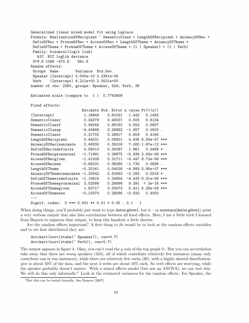
Generalized linear mixed model fit using Laplace
Formula: RealizationOfRecipient ~ SemanticClass + LengthOfRecipient + AnimacyOfRec +
DefinOfRec + PronomOfRec + AccessOfRec + LengthOfTheme + AnimacyOfTheme +
DefinOfTheme + PronomOfTheme + AccessOfTheme + (1 | Speaker) + (1 | Verb)
Family: binomial(logit link)
AIC BIC logLik deviance
979.6 1089 -470.8 941.6
Random effects:
Groups Name Variance Std.Dev.
Speaker (Intercept) 5.000e-10 2.2361e-05
Verb (Intercept) 4.211e+00 2.0521e+00
number of obs: 2360, groups: Speaker, 424; Verb, 38
Estimated scale (compare to 1 ) 0.7743409
Fixed effects:
Estimate Std. Error z value Pr(>|z|)
(Intercept) 1.16849 0.81021 1.442 0.1492
SemanticClassc 0.24379 0.48257 0.505 0.6134
SemanticClassf 0.49244 0.89162 0.552 0.5807
SemanticClassp -4.43666 2.26662 -1.957 0.0503 .
SemanticClasst 0.21702 0.26817 0.809 0.4184
LengthOfRecipient 0.44031 0.08921 4.935 8.00e-07 ***
AnimacyOfRecinanimate 2.49330 0.35316 7.060 1.67e-12 ***
DefinOfRecindefinite 0.59010 0.30097 1.961 0.0499 *
PronomOfRecpronominal -1.71991 0.28975 -5.936 2.92e-09 ***
AccessOfRecgiven -1.41009 0.31711 -4.447 8.72e-06 ***
AccessOfRecnew -0.66231 0.38280 -1.730 0.0836 .
LengthOfTheme -0.20161 0.04038 -4.993 5.95e-07 ***
AnimacyOfThemeinanimate -1.20542 0.52563 -2.293 0.0218 *
DefinOfThemeindefinite -1.10615 0.24954 -4.433 9.31e-06 ***
PronomOfThemepronominal 2.52586 0.26898 9.391 < 2e-16 ***
AccessOfThemegiven 1.62717 0.30073 5.411 6.28e-08 ***
AccessOfThemenew -0.23374 0.28066 -0.833 0.4050
---
Signif. codes: 0 *** 0.001 ** 0.01 * 0.05 . 0.1 1
When doing things, you’ll probably just want to type dative.glmm1, but it – or summary(dative.glmm1) printa very verbose output that also lists correlations between all fixed effects. Here, I use a little trick I learnedfrom Baayen to suppress that output, to keep this handout a little shorter.
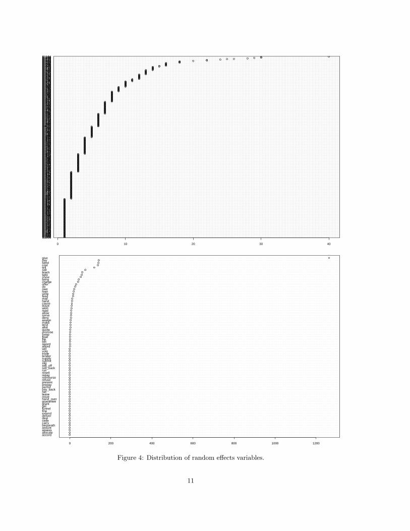
Are the random effects important? A first thing to do would be to look at the random effects variablesand to see how distributed they are:
dotchart(sort(xtabs(~ Speaker)), cex=0.7)
dotchart(sort(xtabs(~ Verb)), cex=0.7)
The output appears in figure 4. Okay, you can’t read the y axis of the top graph /. But you can neverthelesstake away that there are many speakers (424), all of which contribute relatively few instances (many onlycontribute one or two instances), while there are relatively few verbs (38), with a highly skewed distribution:give is about 50% of the data, and the next 3 verbs are about 10% each. So verb effects are worrying, whilethe speaker probably doesn’t matter. With a mixed effects model (but not an ANOVA), we can test this.We will do this only informally.4 Look at the estimated variances for the random effects. For Speaker, the
4But this can be tested formally. See Baayen (2007).
10
S1000S1001S1004S1008S1047S1054S1068S1076S1089S1095S1100S1129S1153S1154S1163S1185S1191S1194S1195S1221S1262S1270S1283S1284S1287S1290S1309S1311S1317S1336S1340S1342S1343S1360S1365S1366S1377S1386S1412S1422S1428S1441S1442S1443S1447S1448S1454S1466S1471S1478S1482S1505S1508S1509S1515S1521S1532S1541S1542S1546S1552S1557S1561S1563S1564S1569S1571S1580S1587S1590S1591S1592S1606S1607S1608S1610S1612S1614S1623S1624S1630S1632S1643S1646S1653S1654S1670S1673S1677S1688S1699S1017S1020S1044S1057S1069S1075S1086S1091S1101S1114S1135S1142S1152S1165S1169S1170S1171S1211S1231S1266S1279S1282S1288S1291S1298S1299S1325S1327S1334S1350S1353S1368S1370S1379S1389S1404S1413S1419S1424S1426S1429S1459S1472S1475S1495S1519S1524S1553S1567S1568S1574S1575S1586S1593S1596S1611S1613S1619S1651S1674S1684S1691S1701S1023S1024S1072S1078S1090S1133S1178S1188S1204S1213S1226S1238S1297S1302S1316S1344S1351S1371S1383S1399S1403S1405S1420S1421S1462S1480S1484S1485S1494S1496S1498S1499S1502S1507S1518S1530S1537S1554S1570S1601S1621S1697S1050S1070S1103S1145S1157S1179S1245S1251S1280S1285S1315S1320S1321S1324S1361S1378S1382S1390S1393S1400S1417S1457S1463S1465S1469S1473S1489S1501S1516S1525S1543S1547S1556S1573S1582S1597S1626S1641S1661S1025S1060S1084S1098S1102S1105S1112S1116S1168S1199S1303S1307S1362S1367S1388S1411S1418S1423S1440S1455S1458S1461S1493S1504S1669S0S1026S1053S1059S1085S1087S1093S1094S1115S1123S1140S1190S1229S1232S1233S1244S1278S1281S1313S1372S1381S1385S1410S1449S1450S1464S1476S1490S1536S1595S1031S1055S1061S1064S1092S1107S1119S1176S1239S1249S1257S1259S1292S1300S1341S1357S1374S1394S1407S1408S1444S1470S1497S1513S1531S1539S1577S1602S1011S1013S1014S1022S1027S1043S1056S1073S1126S1130S1147S1155S1208S1236S1254S1264S1304S1349S1406S1409S1425S1437S1446S1549S1016S1032S1039S1052S1124S1138S1159S1260S1438S1467S1488S1005S1007S1035S1106S1174S1224S1253S1255S1312S1414S1477S1533S1676S1108S1180S1230S1263S1555S1033S1042S1051S1071S1074S1096S1120S1214S1252S1352S1359S1010S1018S1110S1141S1167S1237S1258S1486S1528S1680S1122S1127S1128S1148S1149S1212S1219S1268S1002S1415S1028S1132S1156S1209S1402S1436S1487S1117S1235S1248S1481S1041S1146S1181S1225S1175S1121S1019S1139S1083S1151S1104
0 10 20 30 40
accordallocateassessassurebequeathcarrycededealdeliverextendfinefunnelgetgrantguaranteehand_overissueleasenetpay_backpermitprepaypresentrefusereimburserepayresellrunsell_backsell_offslipsubmitsupplytendertradevotewillaffordawardbetflipfloatswappromisequoteallotlendmakeassigndenyserveallowreadwishleavecausehandmailfeedwriteloanowedoofferchargebringshowtaketeachselltellcostsendpaygive
0 200 400 600 800 1000 1200
Figure 4: Distribution of random effects variables.
11

optimal variance is 5.0e-10 (= 0.0000000005), which is virtually zero: the model gains nothing by attributingthe response to Speaker variation. Speaker isn’t a significant effect in the model. But for Verb, the choiceof verb introduces a large variance (4.2). Hence we can drop the random effect for Speaker. This is great,because model estimation is a ton faster without it ,. Note that we’ve used one of the advantages of aGLMM over an ANOVA. We’ve shown that it is legitimate to ignore Speaker as a random effect for thisdata. As you can see below, fitting the model without Speaker as a random effect makes almost no difference.However, dropping Verb as a random effect makes big differences. (Note that you can’t use lmer() to fit amodel with no random effects – so I revert to lrm() from the Design package.)
> dative.glmm2 <- lmer(RealizationOfRecipient ~ SemanticClass +
LengthOfRecipient + AnimacyOfRec + DefinOfRec + PronomOfRec + AccessOfRec +
LengthOfTheme + AnimacyOfTheme + DefinOfTheme + PronomOfTheme + AccessOfTheme +
(1|Verb), family="binomial")
> print(dative.glmm2, corr=F)
Generalized linear mixed model fit using Laplace
Formula: RealizationOfRecipient ~ SemanticClass + LengthOfRecipient + AnimacyOfRec +
DefinOfRec + PronomOfRec + AccessOfRec + LengthOfTheme + AnimacyOfTheme +
DefinOfTheme + PronomOfTheme + AccessOfTheme + (1 | Verb)
Family: binomial(logit link)
AIC BIC logLik deviance
977.6 1081 -470.8 941.6
Random effects:
Groups Name Variance Std.Dev.
Verb (Intercept) 4.2223 2.0548
number of obs: 2360, groups: Verb, 38
Estimated scale (compare to 1 ) 0.7736354
Fixed effects:
Estimate Std. Error z value Pr(>|z|)
(Intercept) 1.17210 0.81017 1.447 0.1480
SemanticClassc 0.24845 0.48211 0.515 0.6063
SemanticClassf 0.49276 0.89174 0.553 0.5805
SemanticClassp -4.45746 2.27092 -1.963 0.0497 *
SemanticClasst 0.21602 0.26806 0.806 0.4203
LengthOfRecipient 0.43832 0.08903 4.923 8.51e-07 ***
AnimacyOfRecinanimate 2.48833 0.35307 7.048 1.82e-12 ***
DefinOfRecindefinite 0.59095 0.30085 1.964 0.0495 *
PronomOfRecpronominal -1.71852 0.28962 -5.934 2.96e-09 ***
AccessOfRecgiven -1.41119 0.31699 -4.452 8.51e-06 ***
AccessOfRecnew -0.65906 0.38264 -1.722 0.0850 .
LengthOfTheme -0.20108 0.04035 -4.984 6.24e-07 ***
AnimacyOfThemeinanimate -1.20629 0.52556 -2.295 0.0217 *
DefinOfThemeindefinite -1.10467 0.24943 -4.429 9.47e-06 ***
PronomOfThemepronominal 2.52546 0.26892 9.391 < 2e-16 ***
AccessOfThemegiven 1.62756 0.30061 5.414 6.15e-08 ***
AccessOfThemenew -0.23392 0.28055 -0.834 0.4044
---
Signif. codes: 0 *** 0.001 ** 0.01 * 0.05 . 0.1 1
> library(Design)
> dative.dd <- datadist(spdative)
12
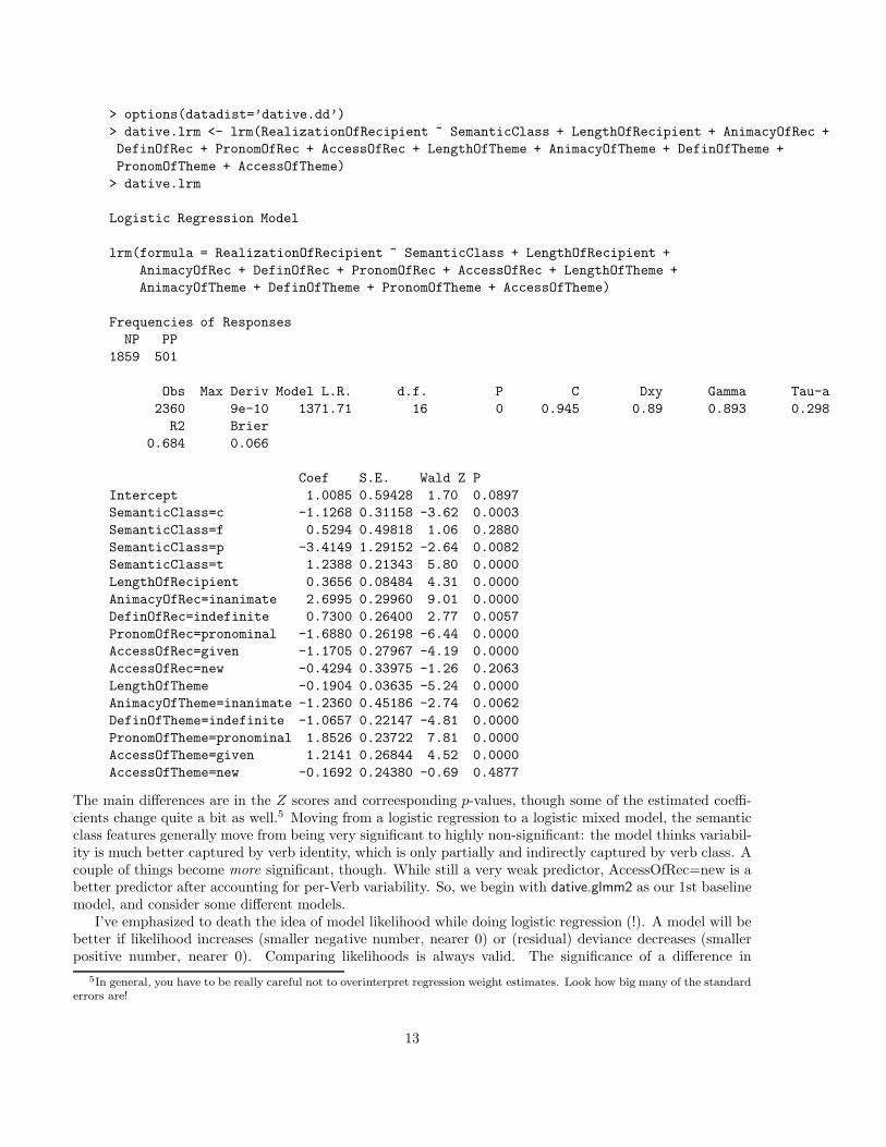
> options(datadist=’dative.dd’)
> dative.lrm <- lrm(RealizationOfRecipient ~ SemanticClass + LengthOfRecipient + AnimacyOfRec +
DefinOfRec + PronomOfRec + AccessOfRec + LengthOfTheme + AnimacyOfTheme + DefinOfTheme +
PronomOfTheme + AccessOfTheme)
> dative.lrm
Logistic Regression Model
lrm(formula = RealizationOfRecipient ~ SemanticClass + LengthOfRecipient +
AnimacyOfRec + DefinOfRec + PronomOfRec + AccessOfRec + LengthOfTheme +
AnimacyOfTheme + DefinOfTheme + PronomOfTheme + AccessOfTheme)
Frequencies of Responses
NP PP
1859 501
Obs Max Deriv Model L.R. d.f. P C Dxy Gamma Tau-a
2360 9e-10 1371.71 16 0 0.945 0.89 0.893 0.298
R2 Brier
0.684 0.066
Coef S.E. Wald Z P
Intercept 1.0085 0.59428 1.70 0.0897
SemanticClass=c -1.1268 0.31158 -3.62 0.0003
SemanticClass=f 0.5294 0.49818 1.06 0.2880
SemanticClass=p -3.4149 1.29152 -2.64 0.0082
SemanticClass=t 1.2388 0.21343 5.80 0.0000
LengthOfRecipient 0.3656 0.08484 4.31 0.0000
AnimacyOfRec=inanimate 2.6995 0.29960 9.01 0.0000
DefinOfRec=indefinite 0.7300 0.26400 2.77 0.0057
PronomOfRec=pronominal -1.6880 0.26198 -6.44 0.0000
AccessOfRec=given -1.1705 0.27967 -4.19 0.0000
AccessOfRec=new -0.4294 0.33975 -1.26 0.2063
LengthOfTheme -0.1904 0.03635 -5.24 0.0000
AnimacyOfTheme=inanimate -1.2360 0.45186 -2.74 0.0062
DefinOfTheme=indefinite -1.0657 0.22147 -4.81 0.0000
PronomOfTheme=pronominal 1.8526 0.23722 7.81 0.0000
AccessOfTheme=given 1.2141 0.26844 4.52 0.0000
AccessOfTheme=new -0.1692 0.24380 -0.69 0.4877
The main differences are in the Z scores and correesponding p-values, though some of the estimated coeffi-cients change quite a bit as well.5 Moving from a logistic regression to a logistic mixed model, the semanticclass features generally move from being very significant to highly non-significant: the model thinks variabil-ity is much better captured by verb identity, which is only partially and indirectly captured by verb class. Acouple of things become more significant, though. While still a very weak predictor, AccessOfRec=new is abetter predictor after accounting for per-Verb variability. So, we begin with dative.glmm2 as our 1st baselinemodel, and consider some different models.
I’ve emphasized to death the idea of model likelihood while doing logistic regression (!). A model will bebetter if likelihood increases (smaller negative number, nearer 0) or (residual) deviance decreases (smallerpositive number, nearer 0). Comparing likelihoods is always valid. The significance of a difference in
5In general, you have to be really careful not to overinterpret regression weight estimates. Look how big many of the standarderrors are!
13

likelihood can be assessed, as before, with the G2 test: testing −2 times the change in likelihood against aχ2 test with the difference in the degrees of freedom.6 However, this time, instead of doing it all by hand,I’ll do it as everyone else does, using the anova() command. I’d avoided it before since it’s an opaque wayto do a simple calculation. But in practice it is the easiest way to do the calculation, so now I’ll use it ,.
But to mention a couple of other criterion, we can also explore model fit by looking at Somers’ Dxy whichgives the rank correlation between predicted probabilities and observed responses. It has a value between 0(random) and 1 (perfect correlation). High is good. While the Design library gives you this as part of theoutput of lrm(), with lme4, you need to calculate it explicitly using the somers2() function.
> somers2(binomial()$linkinv(fitted(dative.glmm2)), as.numeric(RealizationOfRecipient)-1)
C Dxy n Missing
0.9671502 0.9343003 2360.0000000 0.0000000
A final criteria of interest is the Akaike Information Criterion, which is a penalized G2: AIC = G2 − 2 df .The criterion argues for choosing the model that minimizes the AIC. This more strongly favors a simplemodel that captures most of what is going on with the data.
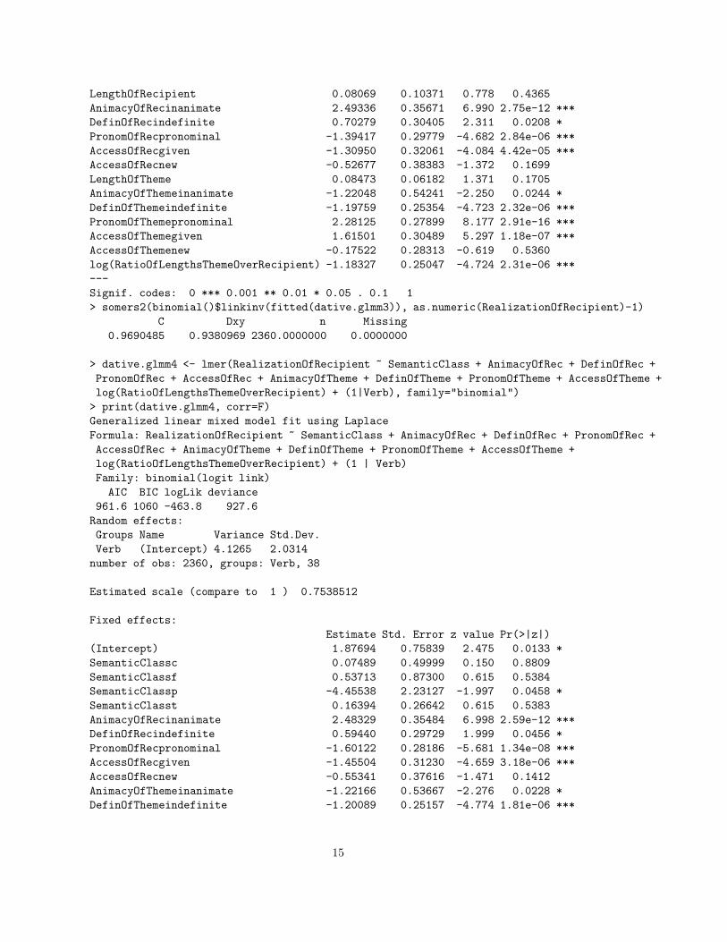
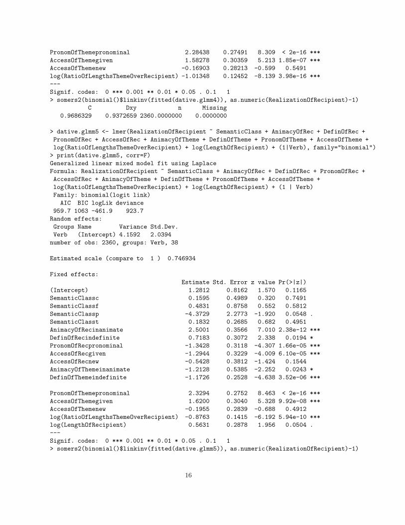
Since I spent so long playing with length models, let me first try if my log ratio length model is better.I could first add it to see if it replaces the others in explanatory effect. It does, as you see below, and themodel is better (dative.glmm3). That is, it’s a little better . . . you can decide whether it was worth the timeI spent. I then delete the plain length factors from the model (dative.glmm4). Adding in the log of one of thelengths, is almost but not quite significant at the 95% level (dative.glmm5), but I would have been resistantto adding it to the model even if it squeaked significance at the 95% level. Adding both log lengths to themodel results in an ill-formed model because the log length ratio is a linear combination of these two factors!lmer() complains.
> dative.glmm3 <- lmer(RealizationOfRecipient ~ SemanticClass + LengthOfRecipient +
AnimacyOfRec + DefinOfRec + PronomOfRec + AccessOfRec + LengthOfTheme + AnimacyOfTheme +
DefinOfTheme + PronomOfTheme + AccessOfTheme + log(RatioOfLengthsThemeOverRecipient) +
(1|Verb), family="binomial")
> print(dative.glmm3, corr=F)
Generalized linear mixed model fit using Laplace
Formula: RealizationOfRecipient ~ SemanticClass + LengthOfRecipient + AnimacyOfRec +
DefinOfRec + PronomOfRec + AccessOfRec + LengthOfTheme + AnimacyOfTheme + DefinOfTheme +
PronomOfTheme + AccessOfTheme + log(RatioOfLengthsThemeOverRecipient) + (1 | Verb)
Family: binomial(logit link)
AIC BIC logLik deviance
960.4 1070 -461.2 922.4
Random effects:
Groups Name Variance Std.Dev.
Verb (Intercept) 4.3188 2.0782
number of obs: 2360, groups: Verb, 38
Estimated scale (compare to 1 ) 0.7457653
Fixed effects:
Estimate Std. Error z value Pr(>|z|)
(Intercept) 1.29310 0.81346 1.590 0.1119
SemanticClassc 0.15628 0.49985 0.313 0.7546
SemanticClassf 0.44694 0.88427 0.505 0.6133
SemanticClassp -4.40247 2.29297 -1.920 0.0549 .
SemanticClasst 0.17068 0.26922 0.634 0.5261
6This test is only necessarily valid for nested models, but in practice it usually works well in all cases where candidate modelsdiffer by just a few degrees of freedom, and so can be used in other cases (Agresti 2002, p. 187).
14
LengthOfRecipient 0.08069 0.10371 0.778 0.4365
AnimacyOfRecinanimate 2.49336 0.35671 6.990 2.75e-12 ***
DefinOfRecindefinite 0.70279 0.30405 2.311 0.0208 *
PronomOfRecpronominal -1.39417 0.29779 -4.682 2.84e-06 ***
AccessOfRecgiven -1.30950 0.32061 -4.084 4.42e-05 ***
AccessOfRecnew -0.52677 0.38383 -1.372 0.1699
LengthOfTheme 0.08473 0.06182 1.371 0.1705
AnimacyOfThemeinanimate -1.22048 0.54241 -2.250 0.0244 *
DefinOfThemeindefinite -1.19759 0.25354 -4.723 2.32e-06 ***
PronomOfThemepronominal 2.28125 0.27899 8.177 2.91e-16 ***
AccessOfThemegiven 1.61501 0.30489 5.297 1.18e-07 ***
AccessOfThemenew -0.17522 0.28313 -0.619 0.5360
log(RatioOfLengthsThemeOverRecipient) -1.18327 0.25047 -4.724 2.31e-06 ***
---
Signif. codes: 0 *** 0.001 ** 0.01 * 0.05 . 0.1 1
> somers2(binomial()$linkinv(fitted(dative.glmm3)), as.numeric(RealizationOfRecipient)-1)
C Dxy n Missing
0.9690485 0.9380969 2360.0000000 0.0000000
> dative.glmm4 <- lmer(RealizationOfRecipient ~ SemanticClass + AnimacyOfRec + DefinOfRec +
PronomOfRec + AccessOfRec + AnimacyOfTheme + DefinOfTheme + PronomOfTheme + AccessOfTheme +
log(RatioOfLengthsThemeOverRecipient) + (1|Verb), family="binomial")
> print(dative.glmm4, corr=F)
Generalized linear mixed model fit using Laplace
Formula: RealizationOfRecipient ~ SemanticClass + AnimacyOfRec + DefinOfRec + PronomOfRec +
AccessOfRec + AnimacyOfTheme + DefinOfTheme + PronomOfTheme + AccessOfTheme +
log(RatioOfLengthsThemeOverRecipient) + (1 | Verb)
Family: binomial(logit link)
AIC BIC logLik deviance
961.6 1060 -463.8 927.6
Random effects:
Groups Name Variance Std.Dev.
Verb (Intercept) 4.1265 2.0314
number of obs: 2360, groups: Verb, 38
Estimated scale (compare to 1 ) 0.7538512
Fixed effects:
Estimate Std. Error z value Pr(>|z|)
(Intercept) 1.87694 0.75839 2.475 0.0133 *
SemanticClassc 0.07489 0.49999 0.150 0.8809
SemanticClassf 0.53713 0.87300 0.615 0.5384
SemanticClassp -4.45538 2.23127 -1.997 0.0458 *
SemanticClasst 0.16394 0.26642 0.615 0.5383
AnimacyOfRecinanimate 2.48329 0.35484 6.998 2.59e-12 ***
DefinOfRecindefinite 0.59440 0.29729 1.999 0.0456 *
PronomOfRecpronominal -1.60122 0.28186 -5.681 1.34e-08 ***
AccessOfRecgiven -1.45504 0.31230 -4.659 3.18e-06 ***
AccessOfRecnew -0.55341 0.37616 -1.471 0.1412
AnimacyOfThemeinanimate -1.22166 0.53667 -2.276 0.0228 *
DefinOfThemeindefinite -1.20089 0.25157 -4.774 1.81e-06 ***
15
PronomOfThemepronominal 2.28438 0.27491 8.309 < 2e-16 ***
AccessOfThemegiven 1.58278 0.30359 5.213 1.85e-07 ***
AccessOfThemenew -0.16903 0.28213 -0.599 0.5491
log(RatioOfLengthsThemeOverRecipient) -1.01348 0.12452 -8.139 3.98e-16 ***
---
Signif. codes: 0 *** 0.001 ** 0.01 * 0.05 . 0.1 1
> somers2(binomial()$linkinv(fitted(dative.glmm4)), as.numeric(RealizationOfRecipient)-1)
C Dxy n Missing
0.9686329 0.9372659 2360.0000000 0.0000000
> dative.glmm5 <- lmer(RealizationOfRecipient ~ SemanticClass + AnimacyOfRec + DefinOfRec +
PronomOfRec + AccessOfRec + AnimacyOfTheme + DefinOfTheme + PronomOfTheme + AccessOfTheme +
log(RatioOfLengthsThemeOverRecipient) + log(LengthOfRecipient) + (1|Verb), family="binomial")
> print(dative.glmm5, corr=F)
Generalized linear mixed model fit using Laplace
Formula: RealizationOfRecipient ~ SemanticClass + AnimacyOfRec + DefinOfRec + PronomOfRec +
AccessOfRec + AnimacyOfTheme + DefinOfTheme + PronomOfTheme + AccessOfTheme +
log(RatioOfLengthsThemeOverRecipient) + log(LengthOfRecipient) + (1 | Verb)
Family: binomial(logit link)
AIC BIC logLik deviance
959.7 1063 -461.9 923.7
Random effects:
Groups Name Variance Std.Dev.
Verb (Intercept) 4.1592 2.0394
number of obs: 2360, groups: Verb, 38
Estimated scale (compare to 1 ) 0.746934
Fixed effects:
Estimate Std. Error z value Pr(>|z|)
(Intercept) 1.2812 0.8162 1.570 0.1165
SemanticClassc 0.1595 0.4989 0.320 0.7491
SemanticClassf 0.4831 0.8758 0.552 0.5812
SemanticClassp -4.3729 2.2773 -1.920 0.0548 .
SemanticClasst 0.1832 0.2685 0.682 0.4951
AnimacyOfRecinanimate 2.5001 0.3566 7.010 2.38e-12 ***
DefinOfRecindefinite 0.7183 0.3072 2.338 0.0194 *
PronomOfRecpronominal -1.3428 0.3118 -4.307 1.66e-05 ***
AccessOfRecgiven -1.2944 0.3229 -4.009 6.10e-05 ***
AccessOfRecnew -0.5428 0.3812 -1.424 0.1544
AnimacyOfThemeinanimate -1.2128 0.5385 -2.252 0.0243 *
DefinOfThemeindefinite -1.1726 0.2528 -4.638 3.52e-06 ***
PronomOfThemepronominal 2.3294 0.2752 8.463 < 2e-16 ***
AccessOfThemegiven 1.6200 0.3040 5.328 9.92e-08 ***
AccessOfThemenew -0.1955 0.2839 -0.688 0.4912
log(RatioOfLengthsThemeOverRecipient) -0.8763 0.1415 -6.192 5.94e-10 ***
log(LengthOfRecipient) 0.5631 0.2878 1.956 0.0504 .
---
Signif. codes: 0 *** 0.001 ** 0.01 * 0.05 . 0.1 1
> somers2(binomial()$linkinv(fitted(dative.glmm5)), as.numeric(RealizationOfRecipient)-1)
16
C Dxy n Missing
0.96894 0.93788 2360.00000 0.00000
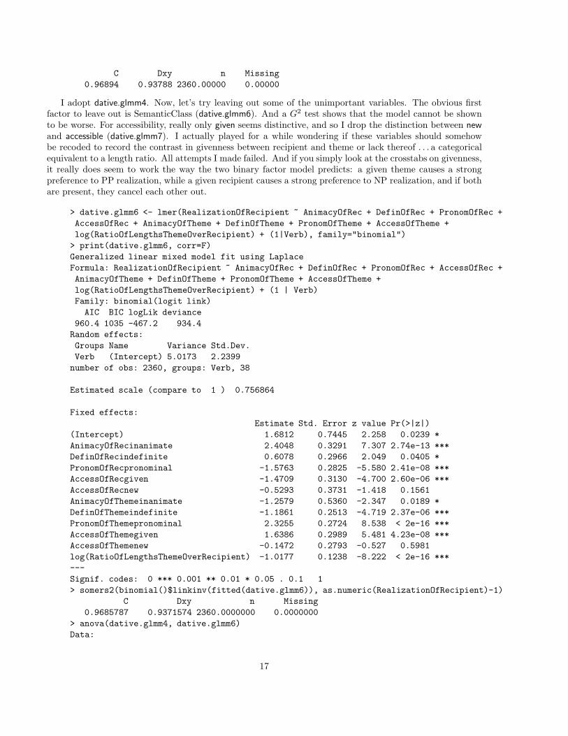
I adopt dative.glmm4. Now, let’s try leaving out some of the unimportant variables. The obvious firstfactor to leave out is SemanticClass (dative.glmm6). And a G2 test shows that the model cannot be shownto be worse. For accessibility, really only given seems distinctive, and so I drop the distinction between newand accessible (dative.glmm7). I actually played for a while wondering if these variables should somehowbe recoded to record the contrast in givenness between recipient and theme or lack thereof . . . a categoricalequivalent to a length ratio. All attempts I made failed. And if you simply look at the crosstabs on givenness,it really does seem to work the way the two binary factor model predicts: a given theme causes a strongpreference to PP realization, while a given recipient causes a strong preference to NP realization, and if bothare present, they cancel each other out.
> dative.glmm6 <- lmer(RealizationOfRecipient ~ AnimacyOfRec + DefinOfRec + PronomOfRec +
AccessOfRec + AnimacyOfTheme + DefinOfTheme + PronomOfTheme + AccessOfTheme +
log(RatioOfLengthsThemeOverRecipient) + (1|Verb), family="binomial")
> print(dative.glmm6, corr=F)
Generalized linear mixed model fit using Laplace
Formula: RealizationOfRecipient ~ AnimacyOfRec + DefinOfRec + PronomOfRec + AccessOfRec +
AnimacyOfTheme + DefinOfTheme + PronomOfTheme + AccessOfTheme +
log(RatioOfLengthsThemeOverRecipient) + (1 | Verb)
Family: binomial(logit link)
AIC BIC logLik deviance
960.4 1035 -467.2 934.4
Random effects:
Groups Name Variance Std.Dev.
Verb (Intercept) 5.0173 2.2399
number of obs: 2360, groups: Verb, 38
Estimated scale (compare to 1 ) 0.756864
Fixed effects:
Estimate Std. Error z value Pr(>|z|)
(Intercept) 1.6812 0.7445 2.258 0.0239 *
AnimacyOfRecinanimate 2.4048 0.3291 7.307 2.74e-13 ***
DefinOfRecindefinite 0.6078 0.2966 2.049 0.0405 *
PronomOfRecpronominal -1.5763 0.2825 -5.580 2.41e-08 ***
AccessOfRecgiven -1.4709 0.3130 -4.700 2.60e-06 ***
AccessOfRecnew -0.5293 0.3731 -1.418 0.1561
AnimacyOfThemeinanimate -1.2579 0.5360 -2.347 0.0189 *
DefinOfThemeindefinite -1.1861 0.2513 -4.719 2.37e-06 ***
PronomOfThemepronominal 2.3255 0.2724 8.538 < 2e-16 ***
AccessOfThemegiven 1.6386 0.2989 5.481 4.23e-08 ***
AccessOfThemenew -0.1472 0.2793 -0.527 0.5981
log(RatioOfLengthsThemeOverRecipient) -1.0177 0.1238 -8.222 < 2e-16 ***
---
Signif. codes: 0 *** 0.001 ** 0.01 * 0.05 . 0.1 1
> somers2(binomial()$linkinv(fitted(dative.glmm6)), as.numeric(RealizationOfRecipient)-1)
C Dxy n Missing
0.9685787 0.9371574 2360.0000000 0.0000000
> anova(dative.glmm4, dative.glmm6)
Data:
17

Models:
dative.glmm6: RealizationOfRecipient ~ AnimacyOfRec + DefinOfRec + PronomOfRec +
dative.glmm4: AccessOfRec + AnimacyOfTheme + DefinOfTheme + PronomOfTheme +
dative.glmm6: AccessOfTheme + log(RatioOfLengthsThemeOverRecipient) + (1 |
dative.glmm4: Verb)
dative.glmm6: RealizationOfRecipient ~ SemanticClass + AnimacyOfRec + DefinOfRec +
dative.glmm4: PronomOfRec + AccessOfRec + AnimacyOfTheme + DefinOfTheme +
dative.glmm6: PronomOfTheme + AccessOfTheme + log(RatioOfLengthsThemeOverRecipient) +
dative.glmm4: (1 | Verb)
Df AIC BIC logLik Chisq Chi Df Pr(>Chisq)
dative.glmm6 13 960.42 1035.38 -467.21
dative.glmm4 17 961.61 1059.63 -463.80 6.8106 4 0.1462
> dative.glmm7 <- lmer(RealizationOfRecipient ~ AnimacyOfRec + DefinOfRec + PronomOfRec +
I(AccessOfRec=="given") + AnimacyOfTheme + DefinOfTheme + PronomOfTheme +
I(AccessOfTheme=="given") + log(RatioOfLengthsThemeOverRecipient) + (1|Verb), family="binomial")
> print(dative.glmm7, corr=F)
Generalized linear mixed model fit using Laplace
Formula: RealizationOfRecipient ~ AnimacyOfRec + DefinOfRec + PronomOfRec +
I(AccessOfRec == "given") + AnimacyOfTheme + DefinOfTheme + PronomOfTheme +
I(AccessOfTheme == "given") + log(RatioOfLengthsThemeOverRecipient) + (1 | Verb)
Family: binomial(logit link)
AIC BIC logLik deviance
959 1022 -468.5 937
Random effects:
Groups Name Variance Std.Dev.
Verb (Intercept) 4.831 2.1980
number of obs: 2360, groups: Verb, 38
Estimated scale (compare to 1 ) 0.7587144
Fixed effects:
Estimate Std. Error z value Pr(>|z|)
(Intercept) 1.5126 0.7272 2.080 0.0375 *
AnimacyOfRecinanimate 2.4003 0.3256 7.373 1.67e-13 ***
DefinOfRecindefinite 0.7071 0.2891 2.446 0.0144 *
PronomOfRecpronominal -1.5265 0.2795 -5.461 4.75e-08 ***
I(AccessOfRec == "given")TRUE -1.3441 0.3018 -4.454 8.44e-06 ***
AnimacyOfThemeinanimate -1.2424 0.5318 -2.336 0.0195 *
DefinOfThemeindefinite -1.2082 0.2498 -4.838 1.31e-06 ***
PronomOfThemepronominal 2.3142 0.2716 8.522 < 2e-16 ***
I(AccessOfTheme == "given")TRUE 1.6337 0.2952 5.535 3.11e-08 ***
log(RatioOfLengthsThemeOverRecipient) -1.0154 0.1238 -8.200 2.41e-16 ***
---
Signif. codes: 0 *** 0.001 ** 0.01 * 0.05 . 0.1 1
> somers2(binomial()$linkinv(fitted(dative.glmm7)), as.numeric(RealizationOfRecipient)-1)
C Dxy n Missing
0.9684595 0.9369191 2360.0000000 0.0000000
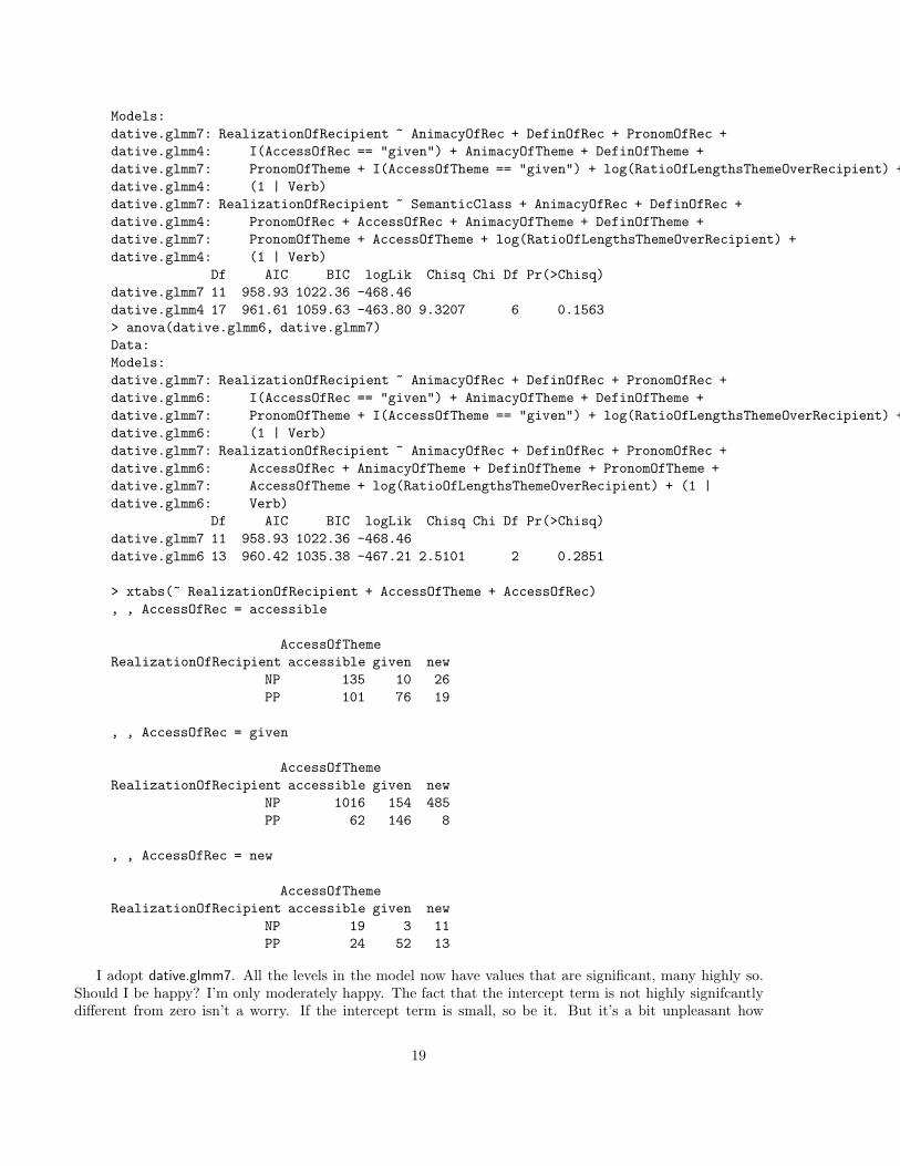
> anova(dative.glmm4, dative.glmm7)
Data:
18
Models:
dative.glmm7: RealizationOfRecipient ~ AnimacyOfRec + DefinOfRec + PronomOfRec +
dative.glmm4: I(AccessOfRec == "given") + AnimacyOfTheme + DefinOfTheme +
dative.glmm7: PronomOfTheme + I(AccessOfTheme == "given") + log(RatioOfLengthsThemeOverRecipient) +
dative.glmm4: (1 | Verb)
dative.glmm7: RealizationOfRecipient ~ SemanticClass + AnimacyOfRec + DefinOfRec +
dative.glmm4: PronomOfRec + AccessOfRec + AnimacyOfTheme + DefinOfTheme +
dative.glmm7: PronomOfTheme + AccessOfTheme + log(RatioOfLengthsThemeOverRecipient) +
dative.glmm4: (1 | Verb)
Df AIC BIC logLik Chisq Chi Df Pr(>Chisq)
dative.glmm7 11 958.93 1022.36 -468.46
dative.glmm4 17 961.61 1059.63 -463.80 9.3207 6 0.1563
> anova(dative.glmm6, dative.glmm7)
Data:
Models:
dative.glmm7: RealizationOfRecipient ~ AnimacyOfRec + DefinOfRec + PronomOfRec +
dative.glmm6: I(AccessOfRec == "given") + AnimacyOfTheme + DefinOfTheme +
dative.glmm7: PronomOfTheme + I(AccessOfTheme == "given") + log(RatioOfLengthsThemeOverRecipient) +
dative.glmm6: (1 | Verb)
dative.glmm7: RealizationOfRecipient ~ AnimacyOfRec + DefinOfRec + PronomOfRec +
dative.glmm6: AccessOfRec + AnimacyOfTheme + DefinOfTheme + PronomOfTheme +
dative.glmm7: AccessOfTheme + log(RatioOfLengthsThemeOverRecipient) + (1 |
dative.glmm6: Verb)
Df AIC BIC logLik Chisq Chi Df Pr(>Chisq)
dative.glmm7 11 958.93 1022.36 -468.46
dative.glmm6 13 960.42 1035.38 -467.21 2.5101 2 0.2851
> xtabs(~ RealizationOfRecipient + AccessOfTheme + AccessOfRec)
, , AccessOfRec = accessible
AccessOfTheme
RealizationOfRecipient accessible given new
NP 135 10 26
PP 101 76 19
, , AccessOfRec = given
AccessOfTheme
RealizationOfRecipient accessible given new
NP 1016 154 485
PP 62 146 8
, , AccessOfRec = new
AccessOfTheme
RealizationOfRecipient accessible given new
NP 19 3 11
PP 24 52 13
I adopt dative.glmm7. All the levels in the model now have values that are significant, many highly so.Should I be happy? I’m only moderately happy. The fact that the intercept term is not highly signifcantlydifferent from zero isn’t a worry. If the intercept term is small, so be it. But it’s a bit unpleasant how
19
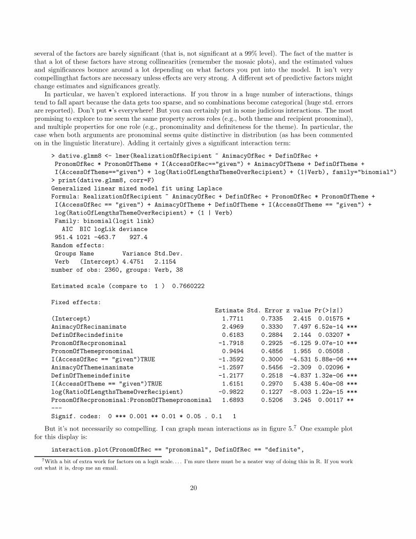
several of the factors are barely significant (that is, not significant at a 99% level). The fact of the matter isthat a lot of these factors have strong collinearities (remember the mosaic plots), and the estimated valuesand significances bounce around a lot depending on what factors you put into the model. It isn’t verycompellingthat factors are necessary unless effects are very strong. A different set of predictive factors mightchange estimates and significances greatly.
In particular, we haven’t explored interactions. If you throw in a huge number of interactions, thingstend to fall apart because the data gets too sparse, and so combinations become categorical (huge std. errorsare reported). Don’t put *’s everywhere! But you can certainly put in some judicious interactions. The mostpromising to explore to me seem the same property across roles (e.g., both theme and recipient pronominal),and multiple properties for one role (e.g., pronominality and definiteness for the theme). In particular, thecase when both arguments are pronominal seems quite distinctive in distribution (as has been commentedon in the linguistic literature). Adding it certainly gives a significant interaction term:
> dative.glmm8 <- lmer(RealizationOfRecipient ~ AnimacyOfRec + DefinOfRec +
PronomOfRec * PronomOfTheme + I(AccessOfRec=="given") + AnimacyOfTheme + DefinOfTheme +
I(AccessOfTheme=="given") + log(RatioOfLengthsThemeOverRecipient) + (1|Verb), family="binomial")
> print(dative.glmm8, corr=F)
Generalized linear mixed model fit using Laplace
Formula: RealizationOfRecipient ~ AnimacyOfRec + DefinOfRec + PronomOfRec * PronomOfTheme +
I(AccessOfRec == "given") + AnimacyOfTheme + DefinOfTheme + I(AccessOfTheme == "given") +
log(RatioOfLengthsThemeOverRecipient) + (1 | Verb)
Family: binomial(logit link)
AIC BIC logLik deviance
951.4 1021 -463.7 927.4
Random effects:
Groups Name Variance Std.Dev.
Verb (Intercept) 4.4751 2.1154
number of obs: 2360, groups: Verb, 38
Estimated scale (compare to 1 ) 0.7660222
Fixed effects:
Estimate Std. Error z value Pr(>|z|)
(Intercept) 1.7711 0.7335 2.415 0.01575 *
AnimacyOfRecinanimate 2.4969 0.3330 7.497 6.52e-14 ***
DefinOfRecindefinite 0.6183 0.2884 2.144 0.03207 *
PronomOfRecpronominal -1.7918 0.2925 -6.125 9.07e-10 ***
PronomOfThemepronominal 0.9494 0.4856 1.955 0.05058 .
I(AccessOfRec == "given")TRUE -1.3592 0.3000 -4.531 5.88e-06 ***
AnimacyOfThemeinanimate -1.2597 0.5456 -2.309 0.02096 *
DefinOfThemeindefinite -1.2177 0.2518 -4.837 1.32e-06 ***
I(AccessOfTheme == "given")TRUE 1.6151 0.2970 5.438 5.40e-08 ***
log(RatioOfLengthsThemeOverRecipient) -0.9822 0.1227 -8.003 1.22e-15 ***
PronomOfRecpronominal:PronomOfThemepronominal 1.6893 0.5206 3.245 0.00117 **
---
Signif. codes: 0 *** 0.001 ** 0.01 * 0.05 . 0.1 1
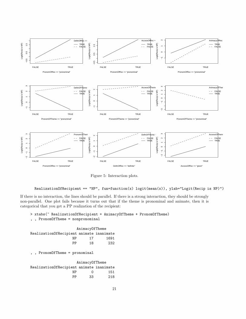
But it’s not necessarily so compelling. I can graph mean interactions as in figure 5.7 One example plotfor this display is:
interaction.plot(PronomOfRec == "pronominal", DefinOfRec == "definite",
7With a bit of extra work for factors on a logit scale. . . . I’m sure there must be a neater way of doing this in R. If you workout what it is, drop me an email.
20
−0.
50.
51.
5
PronomOfRec == "pronominal"
Logi
t(R
ecip
is N
P)
FALSE TRUE
DefinOfRec == "definite"
TRUEFALSE
−0.
50.
51.
5
PronomOfRec == "pronominal"
Logi
t(R
ecip
is N
P)
FALSE TRUE
AccessOfRec == "given"
TRUEFALSE
−1
01
2
PronomOfRec == "pronominal"
Logi
t(R
ecip
is N
P)
FALSE TRUE
AnimacyOfRec == "animate"
TRUEFALSE
−1
01
23
PronomOfTheme == "pronominal"
Logi
t(R
ecip
is N
P)
FALSE TRUE
DefinOfTheme == "definite"
FALSETRUE
−1
01
2
PronomOfTheme == "pronominal"
Logi
t(R
ecip
is N
P)
FALSE TRUE
AccessOfTheme == "given"
FALSETRUE
−3
−1
01
23
PronomOfTheme == "pronominal"
Logi
t(R
ecip
is N
P)
FALSE TRUE
AnimacyOfTheme == "animate"
FALSETRUE
−2
−1
01
23
PronomOfRec == "pronominal"
Logi
t(R
ecip
is N
P)
FALSE TRUE
PronomOfTheme == "pronominal"
FALSETRUE
−2
−1
01
2
DefinOfRec == "definite"
Logi
t(R
ecip
is N
P)
FALSE TRUE
DefinOfTheme == "definite"
FALSETRUE
−2
−1
01
23
AccessOfRec == "given"
Logi
t(R
ecip
is N
P)
FALSE TRUE
AccessOfTheme == "given"
FALSETRUE
Figure 5: Interaction plots.
RealizationOfRecipient == "NP", fun=function(x) logit(mean(x)), ylab="Logit(Recip is NP)")
If there is no interaction, the lines should be parallel. If there is a strong interaction, they should be stronglynon-parallel. One plot fails because it turns out that if the theme is pronominal and animate, then it iscategorical that you get a PP realization of the recipient:
> xtabs(~ RealizationOfRecipient + AnimacyOfTheme + PronomOfTheme)
, , PronomOfTheme = nonpronominal
AnimacyOfTheme
RealizationOfRecipient animate inanimate
NP 17 1691
PP 18 232
, , PronomOfTheme = pronominal
AnimacyOfTheme
RealizationOfRecipient animate inanimate
NP 0 151
PP 33 218
21

I hadn’t realized that! Doing more visualizations almost always leads you to learn more about your data.This clearly shows that there are strong interactions going on for Theme that don’t occur with Recipientor across semantic roles. It turns out to be hard to fully resolve the theme factor interactions becauseof the strong collinearities in the data. It ends up kind of a toss-up whether to put in an interaction ofPronomOfTheme and AccessOfTheme==given or PronomOfTheme and DefinOfTheme. You want one butnot both. I favor the latter because DefinOfTheme seems to have a clearer main effect in the presence of aninteraction term.
If I instead try interaction terms for pronominality and definiteness, for both the theme and recipient, theconjunction is highly significant for the theme but not the recipient. Note that definiteness of the recipienthas now become completely non-significant in this model.
> dative.glmm9 <- lmer(RealizationOfRecipient ~ AnimacyOfRec + DefinOfRec * PronomOfRec +
I(AccessOfRec=="given") + AnimacyOfTheme + DefinOfTheme * PronomOfTheme +
I(AccessOfTheme=="given") + log(RatioOfLengthsThemeOverRecipient) + (1|Verb), family="binomial")
> print(dative.glmm9, corr=F)
Generalized linear mixed model fit using Laplace
Formula: RealizationOfRecipient ~ AnimacyOfRec + DefinOfRec * PronomOfRec +
I(AccessOfRec == "given") + AnimacyOfTheme + DefinOfTheme * PronomOfTheme +
I(AccessOfTheme == "given") + log(RatioOfLengthsThemeOverRecipient) + (1 | Verb)
Family: binomial(logit link)
AIC BIC logLik deviance
919.6 994.5 -446.8 893.6
Random effects:
Groups Name Variance Std.Dev.
Verb (Intercept) 4.9575 2.2265
number of obs: 2360, groups: Verb, 38
Estimated scale (compare to 1 ) 0.7625426
Fixed effects:
Estimate Std. Error z value Pr(>|z|)
(Intercept) 1.5850 0.7714 2.055 0.039906 *
AnimacyOfRecinanimate 2.3007 0.3262 7.052 1.76e-12 ***
DefinOfRecindefinite 0.3549 0.3222 1.101 0.270733
PronomOfRecpronominal -1.8111 0.3268 -5.542 2.99e-08 ***
I(AccessOfRec == "given")TRUE -1.2024 0.3162 -3.802 0.000143 ***
AnimacyOfThemeinanimate -1.3387 0.5831 -2.296 0.021690 *
DefinOfThemeindefinite -0.7497 0.2670 -2.808 0.004978 **
PronomOfThemepronominal 3.9053 0.4055 9.630 < 2e-16 ***
I(AccessOfTheme == "given")TRUE 0.8276 0.3438 2.407 0.016078 *
log(RatioOfLengthsThemeOverRecipient) -0.9433 0.1249 -7.550 4.36e-14 ***
DefinOfRecindefinite:PronomOfRecpronominal 0.8821 0.6303 1.399 0.161684
DefinOfThemeindefinite:PronomOfThemepronominal -4.3583 0.7961 -5.475 4.38e-08 ***
---
Signif. codes: 0 *** 0.001 ** 0.01 * 0.05 . 0.1 1
> dative.glmm10 <- lmer(RealizationOfRecipient ~ AnimacyOfRec + PronomOfRec +
I(AccessOfRec=="given") + AnimacyOfTheme + DefinOfTheme * PronomOfTheme +
I(AccessOfTheme=="given") + log(RatioOfLengthsThemeOverRecipient) + (1|Verb), family="binomial")
> print(dative.glmm10, corr=F)
Generalized linear mixed model fit using Laplace
Formula: RealizationOfRecipient ~ AnimacyOfRec + PronomOfRec + I(AccessOfRec == "given") +
22

AnimacyOfTheme + DefinOfTheme * PronomOfTheme + I(AccessOfTheme == "given") +
log(RatioOfLengthsThemeOverRecipient) + (1 | Verb)
Family: binomial(logit link)
AIC BIC logLik deviance
921.2 984.6 -449.6 899.2
Random effects:
Groups Name Variance Std.Dev.
Verb (Intercept) 5.0413 2.2453
number of obs: 2360, groups: Verb, 38
Estimated scale (compare to 1 ) 0.7754766
Fixed effects:
Estimate Std. Error z value Pr(>|z|)
(Intercept) 1.8436 0.7631 2.416 0.01570 *
AnimacyOfRecinanimate 2.3012 0.3248 7.084 1.40e-12 ***
PronomOfRecpronominal -1.5822 0.2810 -5.631 1.80e-08 ***
I(AccessOfRec == "given")TRUE -1.5588 0.2765 -5.638 1.72e-08 ***
AnimacyOfThemeinanimate -1.4105 0.5786 -2.438 0.01479 *
DefinOfThemeindefinite -0.7494 0.2649 -2.829 0.00467 **
PronomOfThemepronominal 3.9052 0.4040 9.665 < 2e-16 ***
I(AccessOfTheme == "given")TRUE 0.8003 0.3431 2.333 0.01966 *
log(RatioOfLengthsThemeOverRecipient) -0.9366 0.1233 -7.595 3.08e-14 ***
DefinOfThemeindefinite:PronomOfThemepronominal -4.3920 0.7898 -5.561 2.69e-08 ***
---
Signif. codes: 0 *** 0.001 ** 0.01 * 0.05 . 0.1 1
> anova(dative.glmm9, dative.glmm10)
Data:
Models:
dative.glmm10: RealizationOfRecipient ~ AnimacyOfRec + PronomOfRec + I(AccessOfRec ==
dative.glmm9: "given") + AnimacyOfTheme + DefinOfTheme * PronomOfTheme +
dative.glmm10: I(AccessOfTheme == "given") + log(RatioOfLengthsThemeOverRecipient) +
dative.glmm9: (1 | Verb)
dative.glmm10: RealizationOfRecipient ~ AnimacyOfRec + DefinOfRec * PronomOfRec +
dative.glmm9: I(AccessOfRec == "given") + AnimacyOfTheme + DefinOfTheme *
dative.glmm10: PronomOfTheme + I(AccessOfTheme == "given") + log(RatioOfLengthsThemeOverRecipient)
dative.glmm9: (1 | Verb)
Df AIC BIC logLik Chisq Chi Df Pr(>Chisq)
dative.glmm10 11 921.19 984.62 -449.59
dative.glmm9 13 919.57 994.53 -446.78 5.6211 2 0.06017 .
---
Signif. codes: 0 *** 0.001 ** 0.01 * 0.05 . 0.1 1
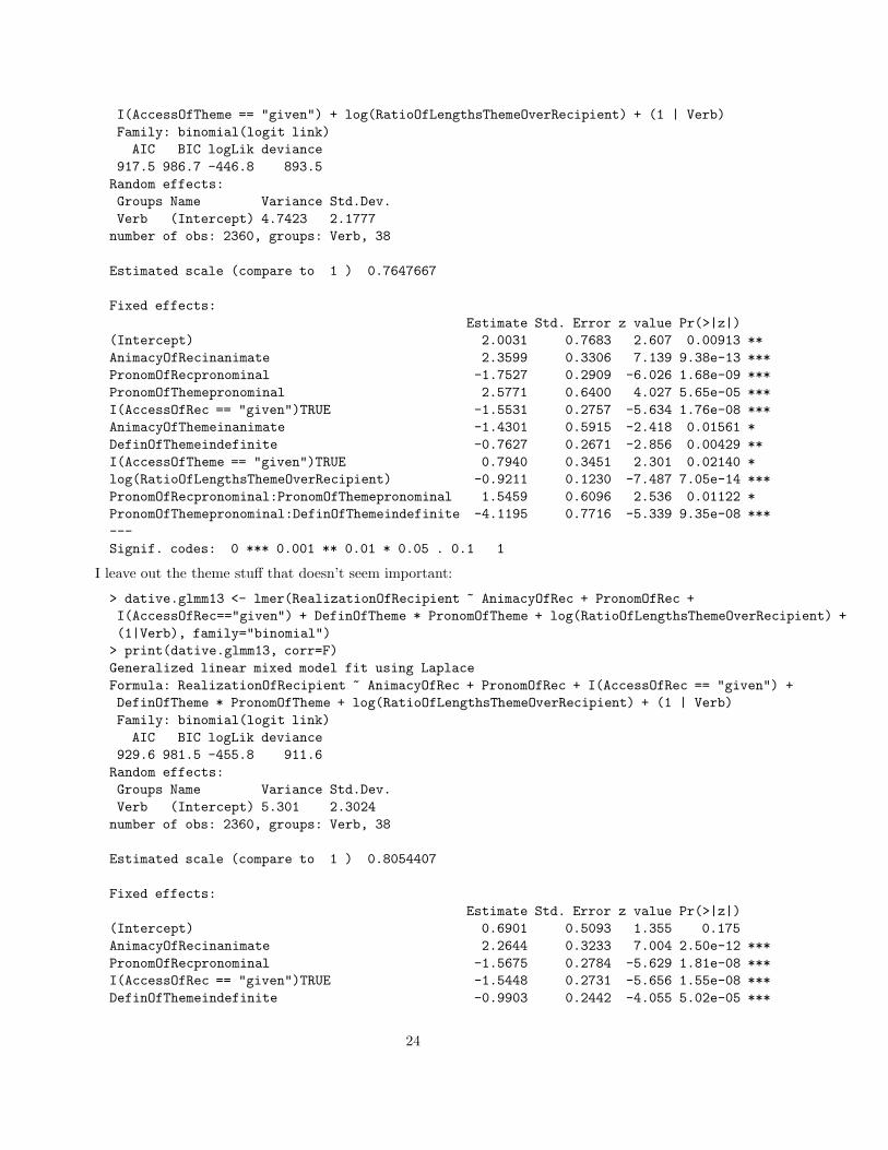
I try putting in both the interactions . . . not so compelling.
> dative.glmm11 <- lmer(RealizationOfRecipient ~ AnimacyOfRec + PronomOfRec * PronomOfTheme +
I(AccessOfRec=="given") + AnimacyOfTheme + DefinOfTheme * PronomOfTheme +
I(AccessOfTheme=="given") + log(RatioOfLengthsThemeOverRecipient) + (1|Verb), family="binomial")
> print(dative.glmm11, corr=F)
Generalized linear mixed model fit using Laplace
Formula: RealizationOfRecipient ~ AnimacyOfRec + PronomOfRec * PronomOfTheme +
I(AccessOfRec == "given") + AnimacyOfTheme + DefinOfTheme * PronomOfTheme +
23
I(AccessOfTheme == "given") + log(RatioOfLengthsThemeOverRecipient) + (1 | Verb)
Family: binomial(logit link)
AIC BIC logLik deviance
917.5 986.7 -446.8 893.5
Random effects:
Groups Name Variance Std.Dev.
Verb (Intercept) 4.7423 2.1777
number of obs: 2360, groups: Verb, 38
Estimated scale (compare to 1 ) 0.7647667
Fixed effects:
Estimate Std. Error z value Pr(>|z|)
(Intercept) 2.0031 0.7683 2.607 0.00913 **
AnimacyOfRecinanimate 2.3599 0.3306 7.139 9.38e-13 ***
PronomOfRecpronominal -1.7527 0.2909 -6.026 1.68e-09 ***
PronomOfThemepronominal 2.5771 0.6400 4.027 5.65e-05 ***
I(AccessOfRec == "given")TRUE -1.5531 0.2757 -5.634 1.76e-08 ***
AnimacyOfThemeinanimate -1.4301 0.5915 -2.418 0.01561 *
DefinOfThemeindefinite -0.7627 0.2671 -2.856 0.00429 **
I(AccessOfTheme == "given")TRUE 0.7940 0.3451 2.301 0.02140 *
log(RatioOfLengthsThemeOverRecipient) -0.9211 0.1230 -7.487 7.05e-14 ***
PronomOfRecpronominal:PronomOfThemepronominal 1.5459 0.6096 2.536 0.01122 *
PronomOfThemepronominal:DefinOfThemeindefinite -4.1195 0.7716 -5.339 9.35e-08 ***
---
Signif. codes: 0 *** 0.001 ** 0.01 * 0.05 . 0.1 1
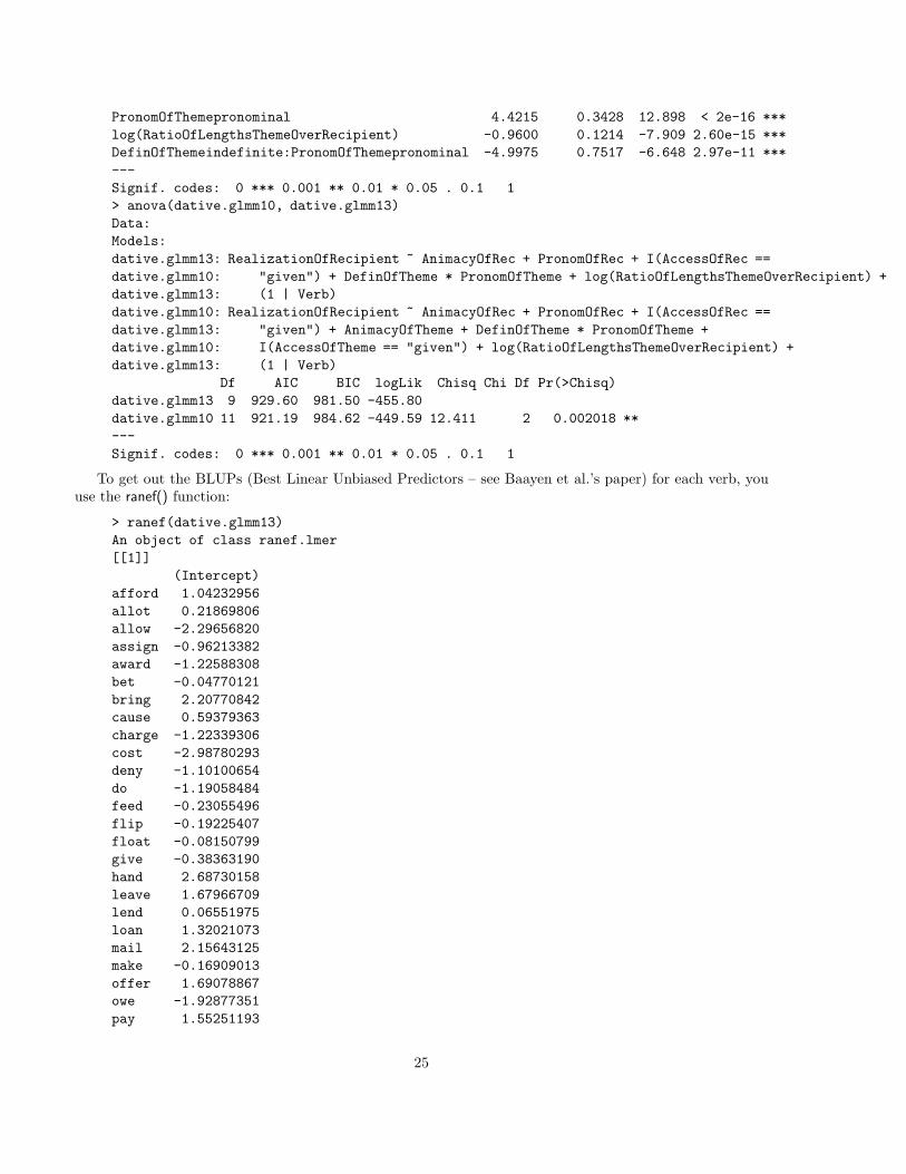
I leave out the theme stuff that doesn’t seem important:
> dative.glmm13 <- lmer(RealizationOfRecipient ~ AnimacyOfRec + PronomOfRec +
I(AccessOfRec=="given") + DefinOfTheme * PronomOfTheme + log(RatioOfLengthsThemeOverRecipient) +
(1|Verb), family="binomial")
> print(dative.glmm13, corr=F)
Generalized linear mixed model fit using Laplace
Formula: RealizationOfRecipient ~ AnimacyOfRec + PronomOfRec + I(AccessOfRec == "given") +
DefinOfTheme * PronomOfTheme + log(RatioOfLengthsThemeOverRecipient) + (1 | Verb)
Family: binomial(logit link)
AIC BIC logLik deviance
929.6 981.5 -455.8 911.6
Random effects:
Groups Name Variance Std.Dev.
Verb (Intercept) 5.301 2.3024
number of obs: 2360, groups: Verb, 38
Estimated scale (compare to 1 ) 0.8054407
Fixed effects:
Estimate Std. Error z value Pr(>|z|)
(Intercept) 0.6901 0.5093 1.355 0.175
AnimacyOfRecinanimate 2.2644 0.3233 7.004 2.50e-12 ***
PronomOfRecpronominal -1.5675 0.2784 -5.629 1.81e-08 ***
I(AccessOfRec == "given")TRUE -1.5448 0.2731 -5.656 1.55e-08 ***
DefinOfThemeindefinite -0.9903 0.2442 -4.055 5.02e-05 ***
24
PronomOfThemepronominal 4.4215 0.3428 12.898 < 2e-16 ***
log(RatioOfLengthsThemeOverRecipient) -0.9600 0.1214 -7.909 2.60e-15 ***
DefinOfThemeindefinite:PronomOfThemepronominal -4.9975 0.7517 -6.648 2.97e-11 ***
---
Signif. codes: 0 *** 0.001 ** 0.01 * 0.05 . 0.1 1
> anova(dative.glmm10, dative.glmm13)
Data:
Models:
dative.glmm13: RealizationOfRecipient ~ AnimacyOfRec + PronomOfRec + I(AccessOfRec ==
dative.glmm10: "given") + DefinOfTheme * PronomOfTheme + log(RatioOfLengthsThemeOverRecipient) +
dative.glmm13: (1 | Verb)
dative.glmm10: RealizationOfRecipient ~ AnimacyOfRec + PronomOfRec + I(AccessOfRec ==
dative.glmm13: "given") + AnimacyOfTheme + DefinOfTheme * PronomOfTheme +
dative.glmm10: I(AccessOfTheme == "given") + log(RatioOfLengthsThemeOverRecipient) +
dative.glmm13: (1 | Verb)
Df AIC BIC logLik Chisq Chi Df Pr(>Chisq)
dative.glmm13 9 929.60 981.50 -455.80
dative.glmm10 11 921.19 984.62 -449.59 12.411 2 0.002018 **
---
Signif. codes: 0 *** 0.001 ** 0.01 * 0.05 . 0.1 1
To get out the BLUPs (Best Linear Unbiased Predictors – see Baayen et al.’s paper) for each verb, youuse the ranef() function:
> ranef(dative.glmm13)
An object of class ranef.lmer
[[1]]
(Intercept)
afford 1.04232956
allot 0.21869806
allow -2.29656820
assign -0.96213382
award -1.22588308
bet -0.04770121
bring 2.20770842
cause 0.59379363
charge -1.22339306
cost -2.98780293
deny -1.10100654
do -1.19058484
feed -0.23055496
flip -0.19225407
float -0.08150799
give -0.38363190
hand 2.68730158
leave 1.67966709
lend 0.06551975
loan 1.32021073
mail 2.15643125
make -0.16909013
offer 1.69078867
owe -1.92877351
pay 1.55251193
25
promise -0.18367423
quote -0.36809443
read 2.22800804
sell 2.01520967
send 1.69002910
serve 1.16722514
show -0.63290084
swap -0.08150799
take 3.32309741
teach -2.63624274
tell -5.02953831
wish -0.66430852
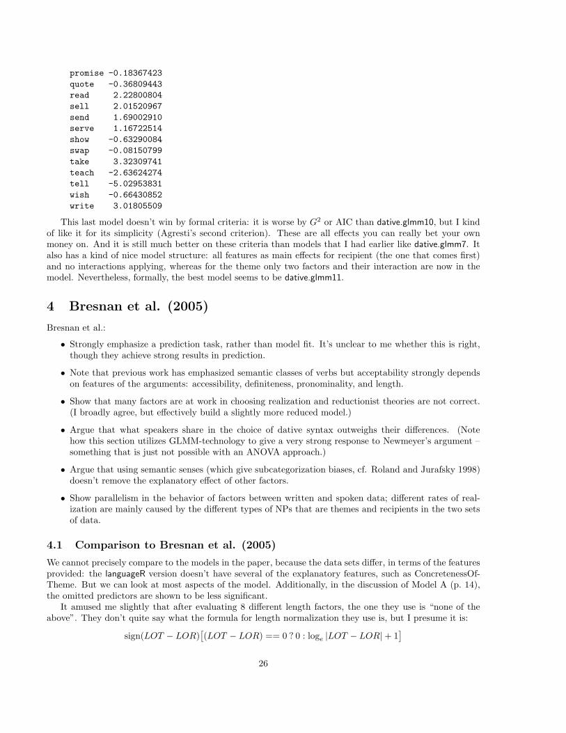
write 3.01805509
This last model doesn’t win by formal criteria: it is worse by G2 or AIC than dative.glmm10, but I kindof like it for its simplicity (Agresti’s second criterion). These are all effects you can really bet your ownmoney on. And it is still much better on these criteria than models that I had earlier like dative.glmm7. Italso has a kind of nice model structure: all features as main effects for recipient (the one that comes first)and no interactions applying, whereas for the theme only two factors and their interaction are now in themodel. Nevertheless, formally, the best model seems to be dative.glmm11.
4 Bresnan et al. (2005)
Bresnan et al.:
• Strongly emphasize a prediction task, rather than model fit. It’s unclear to me whether this is right,though they achieve strong results in prediction.
• Note that previous work has emphasized semantic classes of verbs but acceptability strongly dependson features of the arguments: accessibility, definiteness, pronominality, and length.
• Show that many factors are at work in choosing realization and reductionist theories are not correct.(I broadly agree, but effectively build a slightly more reduced model.)
• Argue that what speakers share in the choice of dative syntax outweighs their differences. (Notehow this section utilizes GLMM-technology to give a very strong response to Newmeyer’s argument –something that is just not possible with an ANOVA approach.)
• Argue that using semantic senses (which give subcategorization biases, cf. Roland and Jurafsky 1998)doesn’t remove the explanatory effect of other factors.
• Show parallelism in the behavior of factors between written and spoken data; different rates of real-ization are mainly caused by the different types of NPs that are themes and recipients in the two setsof data.
4.1 Comparison to Bresnan et al. (2005)
We cannot precisely compare to the models in the paper, because the data sets differ, in terms of the featuresprovided: the languageR version doesn’t have several of the explanatory features, such as ConcretenessOf-Theme. But we can look at most aspects of the model. Additionally, in the discussion of Model A (p. 14),the omitted predictors are shown to be less significant.
It amused me slightly that after evaluating 8 different length factors, the one they use is “none of theabove”. They don’t quite say what the formula for length normalization they use is, but I presume it is:
sign(LOT − LOR)[
(LOT − LOR) == 0 ? 0 : loge|LOT − LOR| + 1
]
26
−3 −2 −1 0 1 2 3 4
−2
−1
01
2
leng.centers4
logi
t(re
l.fre
q.N
P.b
resn
an.le
ng)
Logit ~ Bresnan Length
R2 = 0.92
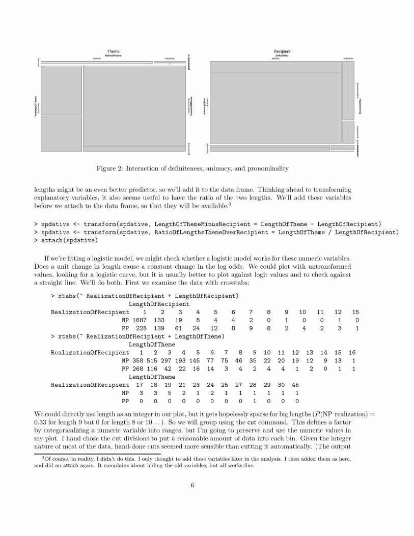
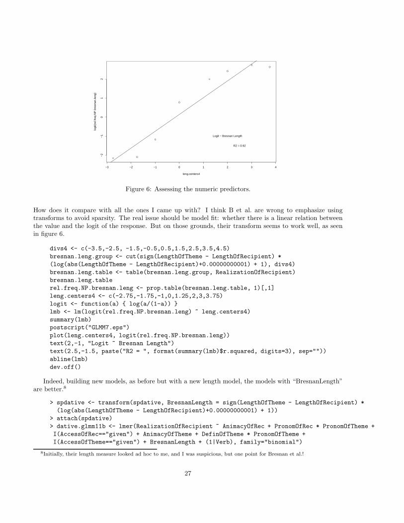
Figure 6: Assessing the numeric predictors.
How does it compare with all the ones I came up with? I think B et al. are wrong to emphasize usingtransforms to avoid sparsity. The real issue should be model fit: whether there is a linear relation betweenthe value and the logit of the response. But on those grounds, their transform seems to work well, as seenin figure 6.
divs4 <- c(-3.5,-2.5, -1.5,-0.5,0.5,1.5,2.5,3.5,4.5)
bresnan.leng.group <- cut(sign(LengthOfTheme - LengthOfRecipient) *
(log(abs(LengthOfTheme - LengthOfRecipient)+0.00000000001) + 1), divs4)
bresnan.leng.table <- table(bresnan.leng.group, RealizationOfRecipient)
bresnan.leng.table
rel.freq.NP.bresnan.leng <- prop.table(bresnan.leng.table, 1)[,1]
leng.centers4 <- c(-2.75,-1.75,-1,0,1.25,2,3,3.75)
logit <- function(a) { log(a/(1-a)) }
lmb <- lm(logit(rel.freq.NP.bresnan.leng) ~ leng.centers4)
summary(lmb)
postscript("GLMM7.eps")
plot(leng.centers4, logit(rel.freq.NP.bresnan.leng))
text(2,-1, "Logit ~ Bresnan Length")
text(2.5,-1.5, paste("R2 = ", format(summary(lmb)$r.squared, digits=3), sep=""))
abline(lmb)
dev.off()
Indeed, building new models, as before but with a new length model, the models with “BresnanLength”are better.8
> spdative <- transform(spdative, BresnanLength = sign(LengthOfTheme - LengthOfRecipient) *
(log(abs(LengthOfTheme - LengthOfRecipient)+0.00000000001) + 1))
> attach(spdative)
> dative.glmm11b <- lmer(RealizationOfRecipient ~ AnimacyOfRec + PronomOfRec * PronomOfTheme +
I(AccessOfRec=="given") + AnimacyOfTheme + DefinOfTheme * PronomOfTheme +
I(AccessOfTheme=="given") + BresnanLength + (1|Verb), family="binomial")
8Initially, their length measure looked ad hoc to me, and I was suspicious, but one point for Bresnan et al.!
27
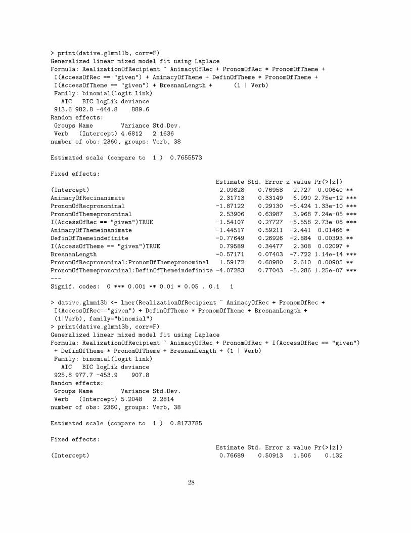
> print(dative.glmm11b, corr=F)
Generalized linear mixed model fit using Laplace
Formula: RealizationOfRecipient ~ AnimacyOfRec + PronomOfRec * PronomOfTheme +
I(AccessOfRec == "given") + AnimacyOfTheme + DefinOfTheme * PronomOfTheme +
I(AccessOfTheme == "given") + BresnanLength + (1 | Verb)
Family: binomial(logit link)
AIC BIC logLik deviance
913.6 982.8 -444.8 889.6
Random effects:
Groups Name Variance Std.Dev.
Verb (Intercept) 4.6812 2.1636
number of obs: 2360, groups: Verb, 38
Estimated scale (compare to 1 ) 0.7655573
Fixed effects:
Estimate Std. Error z value Pr(>|z|)
(Intercept) 2.09828 0.76958 2.727 0.00640 **
AnimacyOfRecinanimate 2.31713 0.33149 6.990 2.75e-12 ***
PronomOfRecpronominal -1.87122 0.29130 -6.424 1.33e-10 ***
PronomOfThemepronominal 2.53906 0.63987 3.968 7.24e-05 ***
I(AccessOfRec == "given")TRUE -1.54107 0.27727 -5.558 2.73e-08 ***
AnimacyOfThemeinanimate -1.44517 0.59211 -2.441 0.01466 *
DefinOfThemeindefinite -0.77649 0.26926 -2.884 0.00393 **
I(AccessOfTheme == "given")TRUE 0.79589 0.34477 2.308 0.02097 *
BresnanLength -0.57171 0.07403 -7.722 1.14e-14 ***
PronomOfRecpronominal:PronomOfThemepronominal 1.59172 0.60980 2.610 0.00905 **
PronomOfThemepronominal:DefinOfThemeindefinite -4.07283 0.77043 -5.286 1.25e-07 ***
---
Signif. codes: 0 *** 0.001 ** 0.01 * 0.05 . 0.1 1
> dative.glmm13b <- lmer(RealizationOfRecipient ~ AnimacyOfRec + PronomOfRec +
I(AccessOfRec=="given") + DefinOfTheme * PronomOfTheme + BresnanLength +
(1|Verb), family="binomial")
> print(dative.glmm13b, corr=F)
Generalized linear mixed model fit using Laplace
Formula: RealizationOfRecipient ~ AnimacyOfRec + PronomOfRec + I(AccessOfRec == "given")
+ DefinOfTheme * PronomOfTheme + BresnanLength + (1 | Verb)
Family: binomial(logit link)
AIC BIC logLik deviance
925.8 977.7 -453.9 907.8
Random effects:
Groups Name Variance Std.Dev.
Verb (Intercept) 5.2048 2.2814
number of obs: 2360, groups: Verb, 38
Estimated scale (compare to 1 ) 0.8173785
Fixed effects:
Estimate Std. Error z value Pr(>|z|)
(Intercept) 0.76689 0.50913 1.506 0.132
28

AnimacyOfRecinanimate 2.22064 0.32397 6.854 7.16e-12 ***
PronomOfRecpronominal -1.68741 0.27935 -6.040 1.54e-09 ***
I(AccessOfRec == "given")TRUE -1.53037 0.27502 -5.565 2.63e-08 ***
DefinOfThemeindefinite -1.00229 0.24596 -4.075 4.60e-05 ***
PronomOfThemepronominal 4.42668 0.34188 12.948 < 2e-16 ***
BresnanLength -0.59528 0.07337 -8.114 4.92e-16 ***
DefinOfThemeindefinite:PronomOfThemepronominal -4.97538 0.75918 -6.554 5.62e-11 ***
---
Signif. codes: 0 *** 0.001 ** 0.01 * 0.05 . 0.1 1
B et al. make some of the same choices as I did, such as collapsing accessibility to given vs. not given.9
We saw the same qualitative harmonic alignment effects as they describe (slightly obscured by the way Rchooses a reference level alphabetically): animate, pronominal, given recipient prefer recipient NP realization(on the negative side of the weight scale). Animate, definite, given or pronominal theme prefer recipient PPrealization (on the positive side of the weight scale).
The nearest analog of the model they present with random effects that we could build is to use all thefixed effects in model B (p. 23) that we have in the data set,10 with a random effect of verb conjoined withsemantic class:11 This does fit the data much better, confirming results of Roland and Jurafsky (1998) thatverb sense strongly effects subcategorization.
> dative.glmmBresnanBprime <- lmer(RealizationOfRecipient ~ SemanticClass +
I(AccessOfRec == "given") + I(AccessOfTheme == "given") + AnimacyOfRec + DefinOfRec +
PronomOfRec + AnimacyOfTheme + DefinOfTheme + PronomOfTheme + BresnanLength - 1 +
(1| Verb:SemanticClass), family="binomial")
> print(dative.glmmBresnanBprime, corr=F)
Generalized linear mixed model fit using Laplace
Formula: RealizationOfRecipient ~ SemanticClass + I(AccessOfRec == "given") +
I(AccessOfTheme == "given") + AnimacyOfRec + DefinOfRec + PronomOfRec + AnimacyOfTheme +
DefinOfTheme + PronomOfTheme + BresnanLength - 1 + (1 | Verb:SemanticClass)
Family: binomial(logit link)
AIC BIC logLik deviance
817.3 903.8 -393.6 787.3
Random effects:
Groups Name Variance Std.Dev.
Verb:SemanticClass (Intercept) 4.808 2.1927
number of obs: 2360, groups: Verb:SemanticClass, 55
Estimated scale (compare to 1 ) 0.7882124
Fixed effects:
Estimate Std. Error z value Pr(>|z|)
SemanticClassa 2.5081 0.9378 2.674 0.007489 **
SemanticClassc 1.1377 1.1004 1.034 0.301198
SemanticClassf 2.3393 1.3232 1.768 0.077073 .
SemanticClassp -2.4542 2.3180 -1.059 0.289707
SemanticClasst 3.3723 0.9245 3.648 0.000265 ***
I(AccessOfRec == "given")TRUE -1.6223 0.3431 -4.728 2.27e-06 ***
I(AccessOfTheme == "given")TRUE 1.4898 0.3258 4.573 4.80e-06 ***
AnimacyOfRecinanimate 1.7389 0.4767 3.648 0.000265 ***
9Though they present this as done in advance to avoid sparsity rather than as a result of model construction.10I leave in AnimacyOfTheme, which they omit, since it probably correlates with ConcretenessOfTheme, which they use.11I use −1 to remove the intercept, as they do, but I really believe it makes no difference here (unlike for a linear regression),
since the intercept term just gets renamed to the otherwise suppressed reference value of the first factor.
29
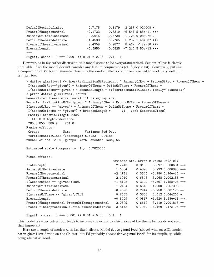
DefinOfRecindefinite 0.7175 0.3179 2.257 0.024008 *
PronomOfRecpronominal -2.1733 0.3319 -6.547 5.85e-11 ***
AnimacyOfThemeinanimate -0.9916 0.5738 -1.728 0.083972 .
DefinOfThemeindefinite -1.4538 0.2765 -5.257 1.46e-07 ***
PronomOfThemepronominal 2.4359 0.2877 8.467 < 2e-16 ***
BresnanLength -0.5950 0.0825 -7.212 5.50e-13 ***
---
Signif. codes: 0 *** 0.001 ** 0.01 * 0.05 . 0.1 1
However, as in my earlier discussion, this model seems to be overparameterized. SemanticClass is clearlyunreliable. And the model doesn’t consider any feature conjunctions (cf. Sigley 2003). Conversely, puttinga conjunction of Verb and SemanticClass into the random effects component seemed to work very well. I’lltry that too:
> dative.glmm11vsci <- lmer(RealizationOfRecipient ~ AnimacyOfRec + PronomOfRec * PronomOfTheme +
I(AccessOfRec=="given") + AnimacyOfTheme + DefinOfTheme * PronomOfTheme +
I(AccessOfTheme=="given") + BresnanLength + (1|Verb:SemanticClass), family="binomial")
> print(dative.glmm11vsci, corr=F)
Generalized linear mixed model fit using Laplace
Formula: RealizationOfRecipient ~ AnimacyOfRec + PronomOfRec * PronomOfTheme +
I(AccessOfRec == "given") + AnimacyOfTheme + DefinOfTheme * PronomOfTheme +
I(AccessOfTheme == "given") + BresnanLength + (1 | Verb:SemanticClass)
Family: binomial(logit link)
AIC BIC logLik deviance
785.8 855 -380.9 761.8
Random effects:
Groups Name Variance Std.Dev.
Verb:SemanticClass (Intercept) 5.8483 2.4183
number of obs: 2360, groups: Verb:SemanticClass, 55
Estimated scale (compare to 1 ) 0.7825365
Fixed effects:
Estimate Std. Error z value Pr(>|z|)
(Intercept) 2.7740 0.8166 3.397 0.000681 ***
AnimacyOfRecinanimate 1.6064 0.4878 3.293 0.000990 ***
PronomOfRecpronominal -2.4741 0.3545 -6.980 2.96e-12 ***
PronomOfThemepronominal 2.1010 0.6848 3.068 0.002155 **
I(AccessOfRec == "given")TRUE -1.8128 0.3199 -5.667 1.45e-08 ***
AnimacyOfThemeinanimate -1.2434 0.6543 -1.900 0.057398 .
DefinOfThemeindefinite -0.9590 0.2944 -3.258 0.001123 **
I(AccessOfTheme == "given")TRUE 0.7655 0.3806 2.012 0.044266 *
BresnanLength -0.5409 0.0817 -6.620 3.58e-11 ***
PronomOfRecpronominal:PronomOfThemepronominal 2.0629 0.6614 3.119 0.001815 **
PronomOfThemepronominal:DefinOfThemeindefinite -3.5173 0.7942 -4.429 9.47e-06 ***
---
Signif. codes: 0 *** 0.001 ** 0.01 * 0.05 . 0.1 1
This model is rather better, but tends to increase the extent to which some of the theme factors do not seemthat important.
Here are a couple of models with less fixed effects. Model dative.glmm11vsci (above) wins on AIC, modeldative.glmm11vsci2 wins on the G2 test, but I’d probably choose dative.glmm11vsci3 for its simplicity, whilebeing almost as good.
30

> dative.glmm11vsci2 <- lmer(RealizationOfRecipient ~ AnimacyOfRec + PronomOfRec * PronomOfTheme +
I(AccessOfRec=="given") + DefinOfTheme * PronomOfTheme + I(AccessOfTheme=="given") +
BresnanLength + (1|Verb:SemanticClass), family="binomial")
> print(dative.glmm11vsci2, corr=F)
Generalized linear mixed model fit using Laplace
Formula: RealizationOfRecipient ~ AnimacyOfRec + PronomOfRec * PronomOfTheme +
I(AccessOfRec == "given") + DefinOfTheme * PronomOfTheme + I(AccessOfTheme == "given") +
BresnanLength + (1 | Verb:SemanticClass)
Family: binomial(logit link)
AIC BIC logLik deviance
787.5 851 -382.8 765.5
Random effects:
Groups Name Variance Std.Dev.
Verb:SemanticClass (Intercept) 6.0148 2.4525
number of obs: 2360, groups: Verb:SemanticClass, 55
Estimated scale (compare to 1 ) 0.791159
Fixed effects:
Estimate Std. Error z value Pr(>|z|)
(Intercept) 1.56744 0.50675 3.093 0.001980 **
AnimacyOfRecinanimate 1.60648 0.48911 3.285 0.001022 **
PronomOfRecpronominal -2.45889 0.35145 -6.996 2.63e-12 ***
PronomOfThemepronominal 2.03569 0.68549 2.970 0.002981 **
I(AccessOfRec == "given")TRUE -1.84243 0.31834 -5.788 7.14e-09 ***
DefinOfThemeindefinite -0.98112 0.29308 -3.348 0.000815 ***
I(AccessOfTheme == "given")TRUE 0.82047 0.37944 2.162 0.030594 *
BresnanLength -0.53505 0.08126 -6.585 4.56e-11 ***
PronomOfRecpronominal:PronomOfThemepronominal 2.07895 0.66271 3.137 0.001707 **
PronomOfThemepronominal:DefinOfThemeindefinite -3.47463 0.79440 -4.374 1.22e-05 ***
---
Signif. codes: 0 *** 0.001 ** 0.01 * 0.05 . 0.1 1
> dative.glmm11vsci3 <- lmer(RealizationOfRecipient ~ AnimacyOfRec + I(AccessOfRec=="given") +
PronomOfRec * PronomOfTheme + DefinOfTheme * PronomOfTheme + BresnanLength + (1|Verb:SemanticClass),
family="binomial")
> print(dative.glmm11vsci3, corr=F)
Generalized linear mixed model fit using Laplace
Formula: RealizationOfRecipient ~ AnimacyOfRec + I(AccessOfRec == "given") +
PronomOfRec * PronomOfTheme + DefinOfTheme * PronomOfTheme + BresnanLength + (1 | Verb:SemanticClass)
Family: binomial(logit link)
AIC BIC logLik deviance
790.1 847.8 -385.0 770.1
Random effects:
Groups Name Variance Std.Dev.
Verb:SemanticClass (Intercept) 6.0267 2.4549
number of obs: 2360, groups: Verb:SemanticClass, 55
Estimated scale (compare to 1 ) 0.8137598
Fixed effects:
31
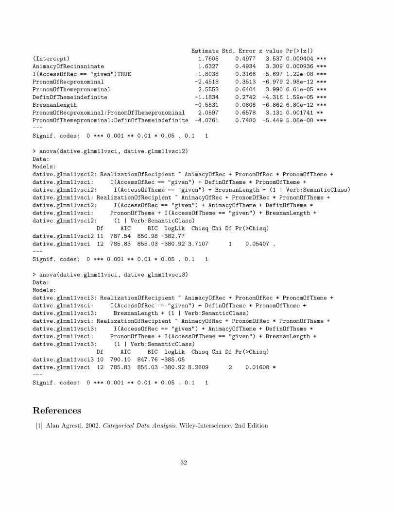
Estimate Std. Error z value Pr(>|z|)
(Intercept) 1.7605 0.4977 3.537 0.000404 ***
AnimacyOfRecinanimate 1.6327 0.4934 3.309 0.000936 ***
I(AccessOfRec == "given")TRUE -1.8038 0.3166 -5.697 1.22e-08 ***
PronomOfRecpronominal -2.4518 0.3513 -6.979 2.98e-12 ***
PronomOfThemepronominal 2.5553 0.6404 3.990 6.61e-05 ***
DefinOfThemeindefinite -1.1834 0.2742 -4.316 1.59e-05 ***
BresnanLength -0.5531 0.0806 -6.862 6.80e-12 ***
PronomOfRecpronominal:PronomOfThemepronominal 2.0597 0.6578 3.131 0.001741 **
PronomOfThemepronominal:DefinOfThemeindefinite -4.0761 0.7480 -5.449 5.06e-08 ***
---
Signif. codes: 0 *** 0.001 ** 0.01 * 0.05 . 0.1 1
> anova(dative.glmm11vsci, dative.glmm11vsci2)
Data:
Models:
dative.glmm11vsci2: RealizationOfRecipient ~ AnimacyOfRec + PronomOfRec * PronomOfTheme +
dative.glmm11vsci: I(AccessOfRec == "given") + DefinOfTheme * PronomOfTheme +
dative.glmm11vsci2: I(AccessOfTheme == "given") + BresnanLength + (1 | Verb:SemanticClass)
dative.glmm11vsci: RealizationOfRecipient ~ AnimacyOfRec + PronomOfRec * PronomOfTheme +
dative.glmm11vsci2: I(AccessOfRec == "given") + AnimacyOfTheme + DefinOfTheme *
dative.glmm11vsci: PronomOfTheme + I(AccessOfTheme == "given") + BresnanLength +
dative.glmm11vsci2: (1 | Verb:SemanticClass)
Df AIC BIC logLik Chisq Chi Df Pr(>Chisq)
dative.glmm11vsci2 11 787.54 850.98 -382.77
dative.glmm11vsci 12 785.83 855.03 -380.92 3.7107 1 0.05407 .
---
Signif. codes: 0 *** 0.001 ** 0.01 * 0.05 . 0.1 1
> anova(dative.glmm11vsci, dative.glmm11vsci3)
Data:
Models:
dative.glmm11vsci3: RealizationOfRecipient ~ AnimacyOfRec + PronomOfRec * PronomOfTheme +
dative.glmm11vsci: I(AccessOfRec == "given") + DefinOfTheme * PronomOfTheme +
dative.glmm11vsci3: BresnanLength + (1 | Verb:SemanticClass)
dative.glmm11vsci: RealizationOfRecipient ~ AnimacyOfRec + PronomOfRec * PronomOfTheme +
dative.glmm11vsci3: I(AccessOfRec == "given") + AnimacyOfTheme + DefinOfTheme *
dative.glmm11vsci: PronomOfTheme + I(AccessOfTheme == "given") + BresnanLength +
dative.glmm11vsci3: (1 | Verb:SemanticClass)
Df AIC BIC logLik Chisq Chi Df Pr(>Chisq)
dative.glmm11vsci3 10 790.10 847.76 -385.05
dative.glmm11vsci 12 785.83 855.03 -380.92 8.2609 2 0.01608 *
---
Signif. codes: 0 *** 0.001 ** 0.01 * 0.05 . 0.1 1
References
[1] Alan Agresti. 2002. Categorical Data Analysis. Wiley-Interscience. 2nd Edition
32

[2] R. Harald Baayen. forthcoming. Analyzing Linguistic Data. A Practical Introduction to Statistics. Cam-bridge University Press.
[3] Baayen, R.H., Davidson, D.J. and Bates, D.M. (submitted). Mixed-effects modeling with crossed randomeffects for subjects and items. MS, 2007.
[4] Joan Bresnan, Anna Cueni, Tatiana Nikitina, and R. Harald Baayen. 2005. Predicting the DativeAlternation. In G. Boume, I. Kraemer, and J. Zwarts (eds.), Cognitive Foundations of Interpretation,Amsterdam: Royal Netherlands Academy of Science, pp. 69–94.
[5] Robert Sigley. 2003. The importance of interaction effects. Language Variation and Change 15: 227–253.
Appendix: Plotting and R-squared for numeric variables
> postscript("GLMM2.eps")
> leng.centers <- c(1,2,3,4,5,6,8.5,12)
> leng.centers2 <- c(-10,-4.5,-3,-2,-1,0,1,2,3,4,5.5,10)
> leng.centers3 <- c(-2,-1.25,-0.75,-0.33,0,0.33,0.75,1.25,1.75,2.25,3)
> logit <- function(a) { log(a/(1-a)) }
> par(mfrow=c(4,4))
>
> lm1 <- lm(rel.freq.NP.theme.leng ~ leng.centers)
> summary(lm1)
Call:
lm(formula = rel.freq.NP.theme.leng ~ leng.centers)
Residuals:
Min 1Q Median 3Q Max
-0.18958 -0.02742 0.02955 0.06465 0.07760
Coefficients:
Estimate Std. Error t value Pr(>|t|)
(Intercept) 0.74193 0.06374 11.640 2.42e-05 ***
leng.centers 0.01954 0.01029 1.899 0.106
---
Signif. codes: 0 *** 0.001 ** 0.01 * 0.05 . 0.1 1
Residual standard error: 0.09864 on 6 degrees of freedom
Multiple R-Squared: 0.3755,Adjusted R-squared: 0.2714
F-statistic: 3.608 on 1 and 6 DF, p-value: 0.1062
> plot(leng.centers, rel.freq.NP.theme.leng)
> text(8,0.7, "Prob ~ Theme Length")
> text(9,0.6, paste("R2 = ", format(summary(lm1)$r.squared, digits=3), sep=""))
> abline(lm1)
> lm2 <- lm(logit(rel.freq.NP.theme.leng) ~ leng.centers)
> summary(lm2)
Call:
lm(formula = logit(rel.freq.NP.theme.leng) ~ leng.centers)
Residuals:
Min 1Q Median 3Q Max
-0.9907 -0.3004 0.2085 0.3966 0.4926
33
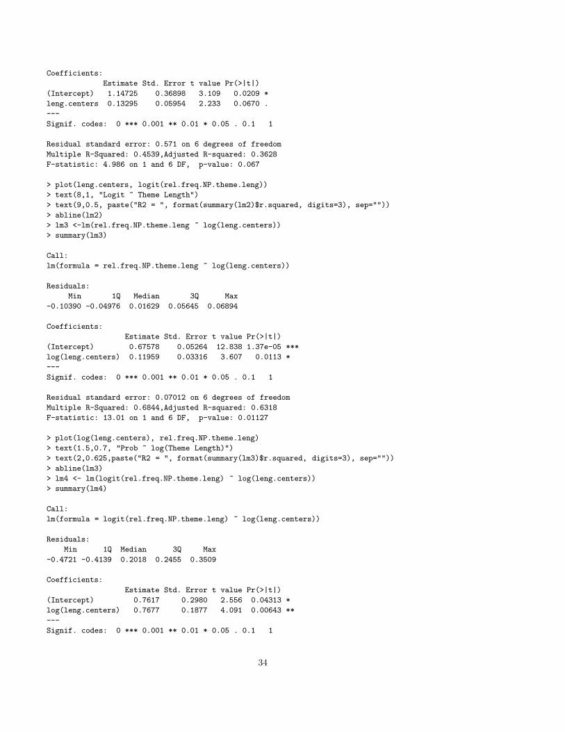
Coefficients:
Estimate Std. Error t value Pr(>|t|)
(Intercept) 1.14725 0.36898 3.109 0.0209 *
leng.centers 0.13295 0.05954 2.233 0.0670 .
---
Signif. codes: 0 *** 0.001 ** 0.01 * 0.05 . 0.1 1
Residual standard error: 0.571 on 6 degrees of freedom
Multiple R-Squared: 0.4539,Adjusted R-squared: 0.3628
F-statistic: 4.986 on 1 and 6 DF, p-value: 0.067
> plot(leng.centers, logit(rel.freq.NP.theme.leng))
> text(8,1, "Logit ~ Theme Length")
> text(9,0.5, paste("R2 = ", format(summary(lm2)$r.squared, digits=3), sep=""))
> abline(lm2)
> lm3 <-lm(rel.freq.NP.theme.leng ~ log(leng.centers))
> summary(lm3)
Call:
lm(formula = rel.freq.NP.theme.leng ~ log(leng.centers))
Residuals:
Min 1Q Median 3Q Max
-0.10390 -0.04976 0.01629 0.05645 0.06894
Coefficients:
Estimate Std. Error t value Pr(>|t|)
(Intercept) 0.67578 0.05264 12.838 1.37e-05 ***
log(leng.centers) 0.11959 0.03316 3.607 0.0113 *
---
Signif. codes: 0 *** 0.001 ** 0.01 * 0.05 . 0.1 1
Residual standard error: 0.07012 on 6 degrees of freedom
Multiple R-Squared: 0.6844,Adjusted R-squared: 0.6318
F-statistic: 13.01 on 1 and 6 DF, p-value: 0.01127
> plot(log(leng.centers), rel.freq.NP.theme.leng)
> text(1.5,0.7, "Prob ~ log(Theme Length)")
> text(2,0.625,paste("R2 = ", format(summary(lm3)$r.squared, digits=3), sep=""))
> abline(lm3)
> lm4 <- lm(logit(rel.freq.NP.theme.leng) ~ log(leng.centers))
> summary(lm4)
Call:
lm(formula = logit(rel.freq.NP.theme.leng) ~ log(leng.centers))
Residuals:
Min 1Q Median 3Q Max
-0.4721 -0.4139 0.2018 0.2455 0.3509
Coefficients:
Estimate Std. Error t value Pr(>|t|)
(Intercept) 0.7617 0.2980 2.556 0.04313 *
log(leng.centers) 0.7677 0.1877 4.091 0.00643 **
---
Signif. codes: 0 *** 0.001 ** 0.01 * 0.05 . 0.1 1
34
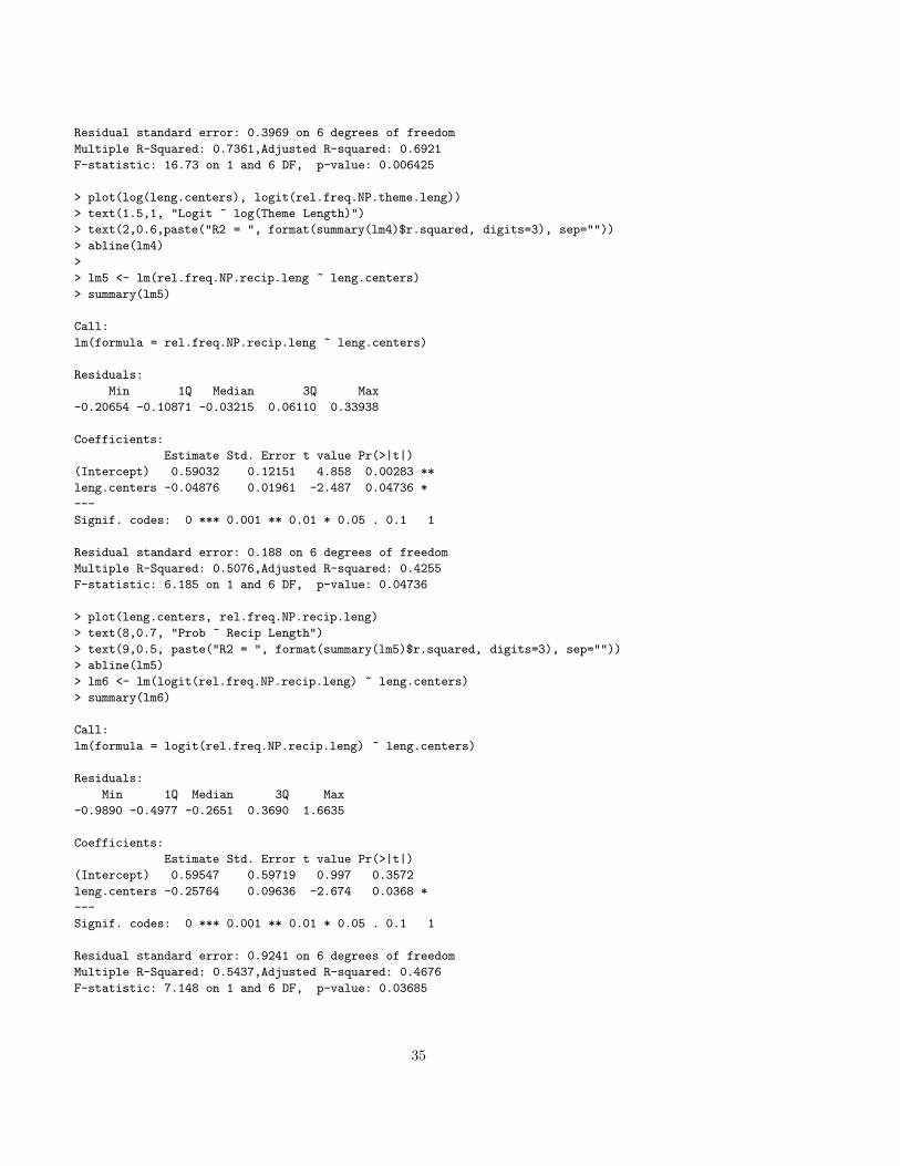
Residual standard error: 0.3969 on 6 degrees of freedom
Multiple R-Squared: 0.7361,Adjusted R-squared: 0.6921
F-statistic: 16.73 on 1 and 6 DF, p-value: 0.006425
> plot(log(leng.centers), logit(rel.freq.NP.theme.leng))
> text(1.5,1, "Logit ~ log(Theme Length)")
> text(2,0.6,paste("R2 = ", format(summary(lm4)$r.squared, digits=3), sep=""))
> abline(lm4)
>
> lm5 <- lm(rel.freq.NP.recip.leng ~ leng.centers)
> summary(lm5)
Call:
lm(formula = rel.freq.NP.recip.leng ~ leng.centers)
Residuals:
Min 1Q Median 3Q Max
-0.20654 -0.10871 -0.03215 0.06110 0.33938
Coefficients:
Estimate Std. Error t value Pr(>|t|)
(Intercept) 0.59032 0.12151 4.858 0.00283 **
leng.centers -0.04876 0.01961 -2.487 0.04736 *
---
Signif. codes: 0 *** 0.001 ** 0.01 * 0.05 . 0.1 1
Residual standard error: 0.188 on 6 degrees of freedom
Multiple R-Squared: 0.5076,Adjusted R-squared: 0.4255
F-statistic: 6.185 on 1 and 6 DF, p-value: 0.04736
> plot(leng.centers, rel.freq.NP.recip.leng)
> text(8,0.7, "Prob ~ Recip Length")
> text(9,0.5, paste("R2 = ", format(summary(lm5)$r.squared, digits=3), sep=""))
> abline(lm5)
> lm6 <- lm(logit(rel.freq.NP.recip.leng) ~ leng.centers)
> summary(lm6)
Call:
lm(formula = logit(rel.freq.NP.recip.leng) ~ leng.centers)
Residuals:
Min 1Q Median 3Q Max
-0.9890 -0.4977 -0.2651 0.3690 1.6635
Coefficients:
Estimate Std. Error t value Pr(>|t|)
(Intercept) 0.59547 0.59719 0.997 0.3572
leng.centers -0.25764 0.09636 -2.674 0.0368 *
---
Signif. codes: 0 *** 0.001 ** 0.01 * 0.05 . 0.1 1
Residual standard error: 0.9241 on 6 degrees of freedom
Multiple R-Squared: 0.5437,Adjusted R-squared: 0.4676
F-statistic: 7.148 on 1 and 6 DF, p-value: 0.03685
35
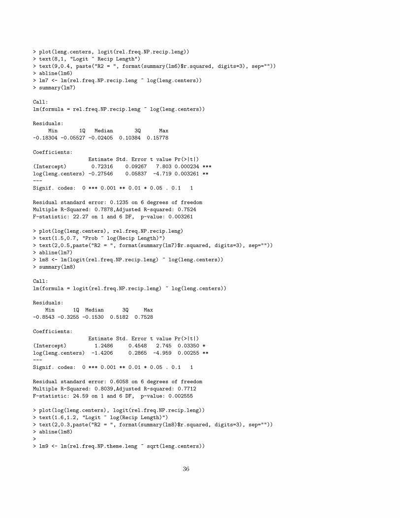
> plot(leng.centers, logit(rel.freq.NP.recip.leng))
> text(8,1, "Logit ~ Recip Length")
> text(9,0.4, paste("R2 = ", format(summary(lm6)$r.squared, digits=3), sep=""))
> abline(lm6)
> lm7 <- lm(rel.freq.NP.recip.leng ~ log(leng.centers))
> summary(lm7)
Call:
lm(formula = rel.freq.NP.recip.leng ~ log(leng.centers))
Residuals:
Min 1Q Median 3Q Max
-0.18304 -0.05527 -0.02405 0.10384 0.15778
Coefficients:
Estimate Std. Error t value Pr(>|t|)
(Intercept) 0.72316 0.09267 7.803 0.000234 ***
log(leng.centers) -0.27546 0.05837 -4.719 0.003261 **
---
Signif. codes: 0 *** 0.001 ** 0.01 * 0.05 . 0.1 1
Residual standard error: 0.1235 on 6 degrees of freedom
Multiple R-Squared: 0.7878,Adjusted R-squared: 0.7524
F-statistic: 22.27 on 1 and 6 DF, p-value: 0.003261
> plot(log(leng.centers), rel.freq.NP.recip.leng)
> text(1.5,0.7, "Prob ~ log(Recip Length)")
> text(2,0.5,paste("R2 = ", format(summary(lm7)$r.squared, digits=3), sep=""))
> abline(lm7)
> lm8 <- lm(logit(rel.freq.NP.recip.leng) ~ log(leng.centers))
> summary(lm8)
Call:
lm(formula = logit(rel.freq.NP.recip.leng) ~ log(leng.centers))
Residuals:
Min 1Q Median 3Q Max
-0.8543 -0.3255 -0.1530 0.5182 0.7528
Coefficients:
Estimate Std. Error t value Pr(>|t|)
(Intercept) 1.2486 0.4548 2.745 0.03350 *
log(leng.centers) -1.4206 0.2865 -4.959 0.00255 **
---
Signif. codes: 0 *** 0.001 ** 0.01 * 0.05 . 0.1 1
Residual standard error: 0.6058 on 6 degrees of freedom
Multiple R-Squared: 0.8039,Adjusted R-squared: 0.7712
F-statistic: 24.59 on 1 and 6 DF, p-value: 0.002555
> plot(log(leng.centers), logit(rel.freq.NP.recip.leng))
> text(1.6,1.2, "Logit ~ log(Recip Length)")
> text(2,0.3,paste("R2 = ", format(summary(lm8)$r.squared, digits=3), sep=""))
> abline(lm8)
>
> lm9 <- lm(rel.freq.NP.theme.leng ~ sqrt(leng.centers))
36
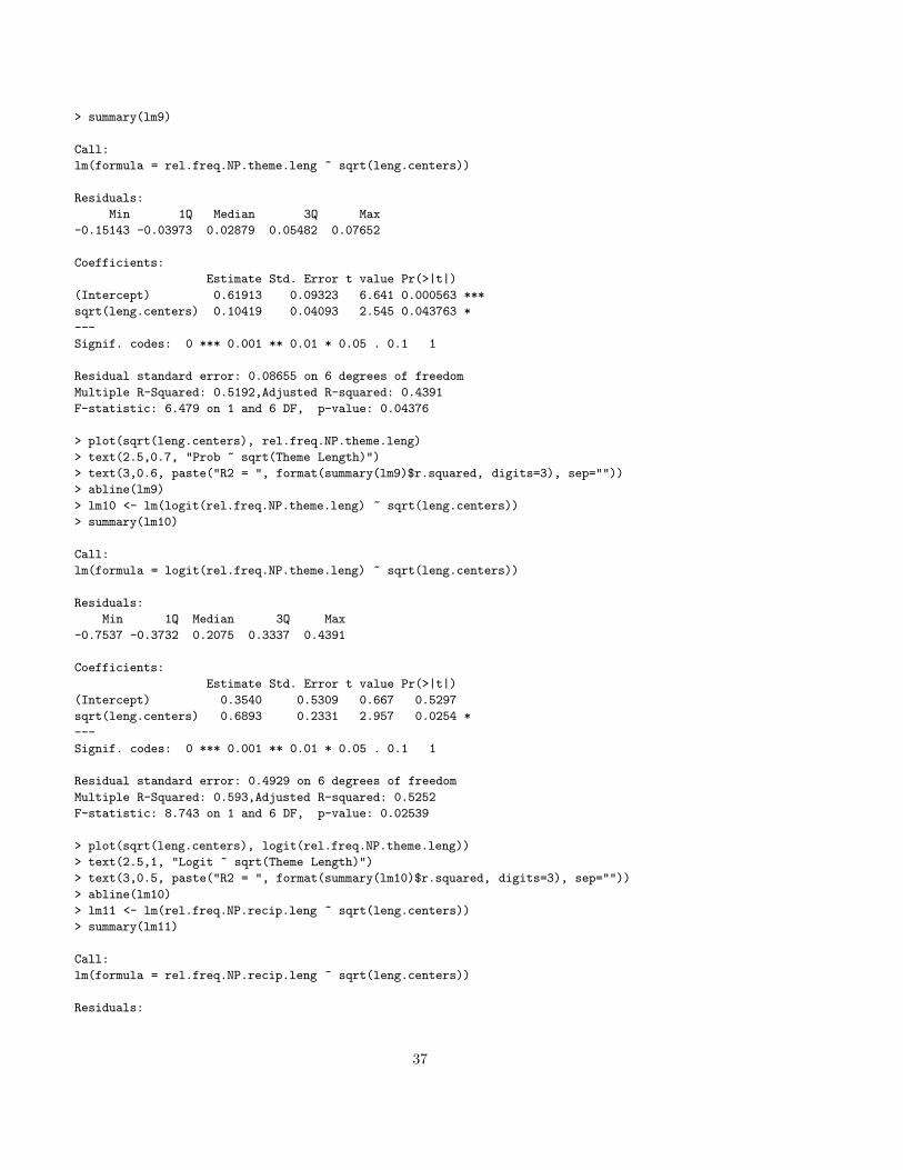
> summary(lm9)
Call:
lm(formula = rel.freq.NP.theme.leng ~ sqrt(leng.centers))
Residuals:
Min 1Q Median 3Q Max
-0.15143 -0.03973 0.02879 0.05482 0.07652
Coefficients:
Estimate Std. Error t value Pr(>|t|)
(Intercept) 0.61913 0.09323 6.641 0.000563 ***
sqrt(leng.centers) 0.10419 0.04093 2.545 0.043763 *
---
Signif. codes: 0 *** 0.001 ** 0.01 * 0.05 . 0.1 1
Residual standard error: 0.08655 on 6 degrees of freedom
Multiple R-Squared: 0.5192,Adjusted R-squared: 0.4391
F-statistic: 6.479 on 1 and 6 DF, p-value: 0.04376
> plot(sqrt(leng.centers), rel.freq.NP.theme.leng)
> text(2.5,0.7, "Prob ~ sqrt(Theme Length)")
> text(3,0.6, paste("R2 = ", format(summary(lm9)$r.squared, digits=3), sep=""))
> abline(lm9)
> lm10 <- lm(logit(rel.freq.NP.theme.leng) ~ sqrt(leng.centers))
> summary(lm10)
Call:
lm(formula = logit(rel.freq.NP.theme.leng) ~ sqrt(leng.centers))
Residuals:
Min 1Q Median 3Q Max
-0.7537 -0.3732 0.2075 0.3337 0.4391
Coefficients:
Estimate Std. Error t value Pr(>|t|)
(Intercept) 0.3540 0.5309 0.667 0.5297
sqrt(leng.centers) 0.6893 0.2331 2.957 0.0254 *
---
Signif. codes: 0 *** 0.001 ** 0.01 * 0.05 . 0.1 1
Residual standard error: 0.4929 on 6 degrees of freedom
Multiple R-Squared: 0.593,Adjusted R-squared: 0.5252
F-statistic: 8.743 on 1 and 6 DF, p-value: 0.02539
> plot(sqrt(leng.centers), logit(rel.freq.NP.theme.leng))
> text(2.5,1, "Logit ~ sqrt(Theme Length)")
> text(3,0.5, paste("R2 = ", format(summary(lm10)$r.squared, digits=3), sep=""))
> abline(lm10)
> lm11 <- lm(rel.freq.NP.recip.leng ~ sqrt(leng.centers))
> summary(lm11)
Call:
lm(formula = rel.freq.NP.recip.leng ~ sqrt(leng.centers))
Residuals:
37
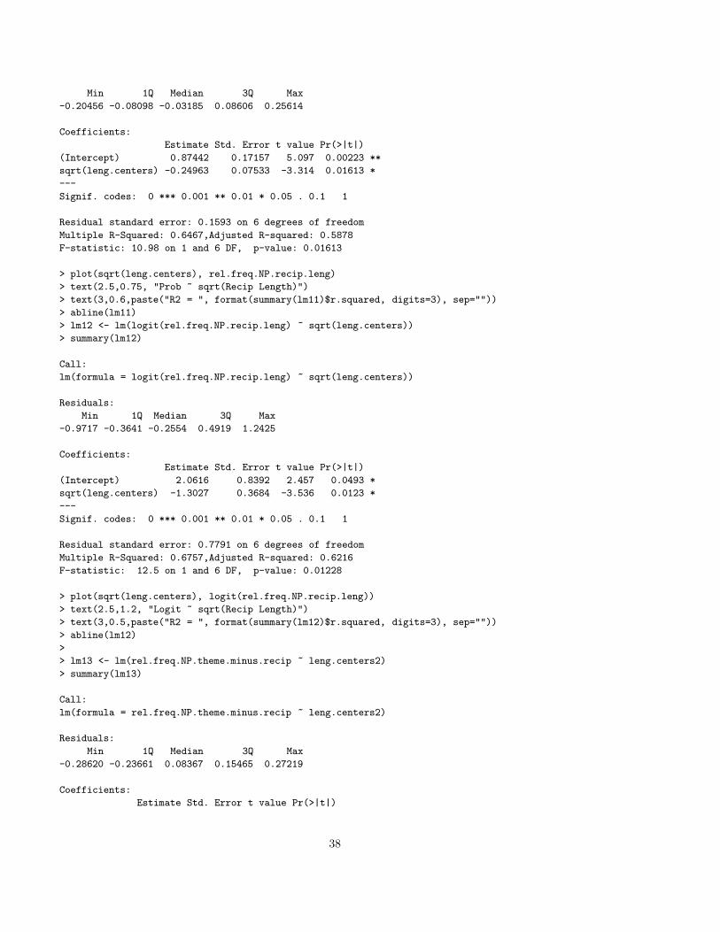
Min 1Q Median 3Q Max
-0.20456 -0.08098 -0.03185 0.08606 0.25614
Coefficients:
Estimate Std. Error t value Pr(>|t|)
(Intercept) 0.87442 0.17157 5.097 0.00223 **
sqrt(leng.centers) -0.24963 0.07533 -3.314 0.01613 *
---
Signif. codes: 0 *** 0.001 ** 0.01 * 0.05 . 0.1 1
Residual standard error: 0.1593 on 6 degrees of freedom
Multiple R-Squared: 0.6467,Adjusted R-squared: 0.5878
F-statistic: 10.98 on 1 and 6 DF, p-value: 0.01613
> plot(sqrt(leng.centers), rel.freq.NP.recip.leng)
> text(2.5,0.75, "Prob ~ sqrt(Recip Length)")
> text(3,0.6,paste("R2 = ", format(summary(lm11)$r.squared, digits=3), sep=""))
> abline(lm11)
> lm12 <- lm(logit(rel.freq.NP.recip.leng) ~ sqrt(leng.centers))
> summary(lm12)
Call:
lm(formula = logit(rel.freq.NP.recip.leng) ~ sqrt(leng.centers))
Residuals:
Min 1Q Median 3Q Max
-0.9717 -0.3641 -0.2554 0.4919 1.2425
Coefficients:
Estimate Std. Error t value Pr(>|t|)
(Intercept) 2.0616 0.8392 2.457 0.0493 *
sqrt(leng.centers) -1.3027 0.3684 -3.536 0.0123 *
---
Signif. codes: 0 *** 0.001 ** 0.01 * 0.05 . 0.1 1
Residual standard error: 0.7791 on 6 degrees of freedom
Multiple R-Squared: 0.6757,Adjusted R-squared: 0.6216
F-statistic: 12.5 on 1 and 6 DF, p-value: 0.01228
> plot(sqrt(leng.centers), logit(rel.freq.NP.recip.leng))
> text(2.5,1.2, "Logit ~ sqrt(Recip Length)")
> text(3,0.5,paste("R2 = ", format(summary(lm12)$r.squared, digits=3), sep=""))
> abline(lm12)
>
> lm13 <- lm(rel.freq.NP.theme.minus.recip ~ leng.centers2)
> summary(lm13)
Call:
lm(formula = rel.freq.NP.theme.minus.recip ~ leng.centers2)
Residuals:
Min 1Q Median 3Q Max
-0.28620 -0.23661 0.08367 0.15465 0.27219
Coefficients:
Estimate Std. Error t value Pr(>|t|)
38
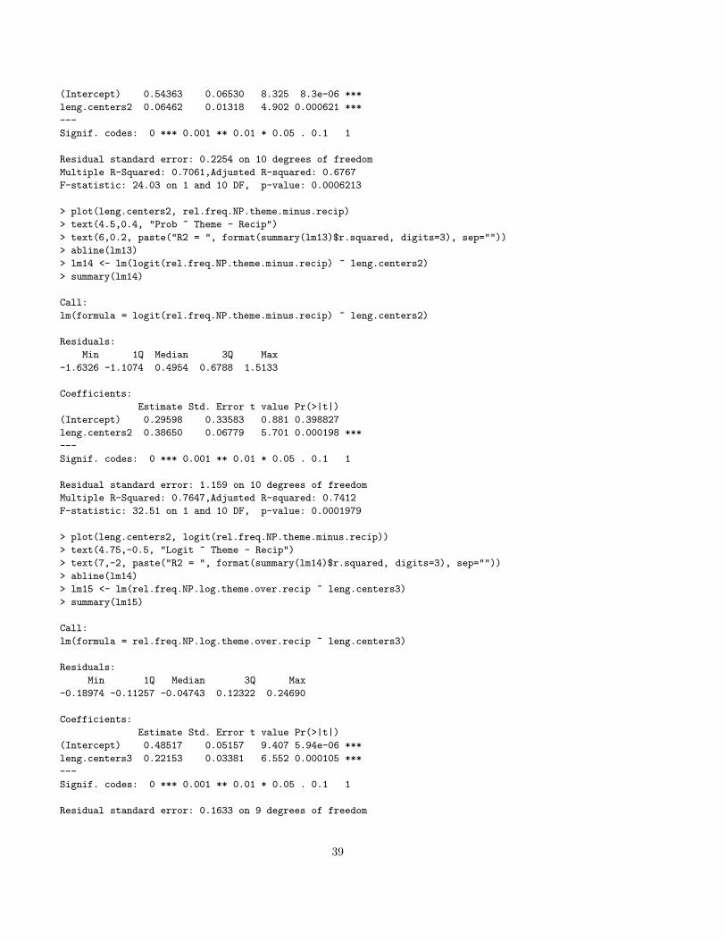
(Intercept) 0.54363 0.06530 8.325 8.3e-06 ***
leng.centers2 0.06462 0.01318 4.902 0.000621 ***
---
Signif. codes: 0 *** 0.001 ** 0.01 * 0.05 . 0.1 1
Residual standard error: 0.2254 on 10 degrees of freedom
Multiple R-Squared: 0.7061,Adjusted R-squared: 0.6767
F-statistic: 24.03 on 1 and 10 DF, p-value: 0.0006213
> plot(leng.centers2, rel.freq.NP.theme.minus.recip)
> text(4.5,0.4, "Prob ~ Theme - Recip")
> text(6,0.2, paste("R2 = ", format(summary(lm13)$r.squared, digits=3), sep=""))
> abline(lm13)
> lm14 <- lm(logit(rel.freq.NP.theme.minus.recip) ~ leng.centers2)
> summary(lm14)
Call:
lm(formula = logit(rel.freq.NP.theme.minus.recip) ~ leng.centers2)
Residuals:
Min 1Q Median 3Q Max
-1.6326 -1.1074 0.4954 0.6788 1.5133
Coefficients:
Estimate Std. Error t value Pr(>|t|)
(Intercept) 0.29598 0.33583 0.881 0.398827
leng.centers2 0.38650 0.06779 5.701 0.000198 ***
---
Signif. codes: 0 *** 0.001 ** 0.01 * 0.05 . 0.1 1
Residual standard error: 1.159 on 10 degrees of freedom
Multiple R-Squared: 0.7647,Adjusted R-squared: 0.7412
F-statistic: 32.51 on 1 and 10 DF, p-value: 0.0001979
> plot(leng.centers2, logit(rel.freq.NP.theme.minus.recip))
> text(4.75,-0.5, "Logit ~ Theme - Recip")
> text(7,-2, paste("R2 = ", format(summary(lm14)$r.squared, digits=3), sep=""))
> abline(lm14)
> lm15 <- lm(rel.freq.NP.log.theme.over.recip ~ leng.centers3)
> summary(lm15)
Call:
lm(formula = rel.freq.NP.log.theme.over.recip ~ leng.centers3)
Residuals:
Min 1Q Median 3Q Max
-0.18974 -0.11257 -0.04743 0.12322 0.24690
Coefficients:
Estimate Std. Error t value Pr(>|t|)
(Intercept) 0.48517 0.05157 9.407 5.94e-06 ***
leng.centers3 0.22153 0.03381 6.552 0.000105 ***
---
Signif. codes: 0 *** 0.001 ** 0.01 * 0.05 . 0.1 1
Residual standard error: 0.1633 on 9 degrees of freedom
39

Multiple R-Squared: 0.8267,Adjusted R-squared: 0.8074
F-statistic: 42.92 on 1 and 9 DF, p-value: 0.0001050
> plot(leng.centers3, rel.freq.NP.log.theme.over.recip)
> text(1.5,0.175, "Prob ~ log(Theme/Recip)")
> text(2,0.4, paste("R2 = ", format(summary(lm15)$r.squared, digits=3), sep=""))
> abline(lm15)
> lm16 <- lm(logit(rel.freq.NP.log.theme.over.recip) ~ leng.centers3)
> summary(lm16)
Call:
lm(formula = logit(rel.freq.NP.log.theme.over.recip) ~ leng.centers3)
Residuals:
Min 1Q Median 3Q Max
-0.8650 -0.6090 -0.3581 0.6503 1.1329
Coefficients:
Estimate Std. Error t value Pr(>|t|)
(Intercept) 0.04521 0.24371 0.186 0.857
leng.centers3 1.33263 0.15978 8.341 1.58e-05 ***
---
Signif. codes: 0 *** 0.001 ** 0.01 * 0.05 . 0.1 1
Residual standard error: 0.7716 on 9 degrees of freedom
Multiple R-Squared: 0.8854,Adjusted R-squared: 0.8727
F-statistic: 69.57 on 1 and 9 DF, p-value: 1.584e-05
> plot(leng.centers3, logit(rel.freq.NP.log.theme.over.recip))
> text(1.5,-1.5, "Logit ~ log(Theme/Recip)")
> text(2,0, paste("R2 = ", format(summary(lm16)$r.squared, digits=3), sep=""))
> abline(lm16)
> dev.off()
quartz
2
40