generalized ornstein-uhlenbeck processes and infinite
TRANSCRIPT

Publ. RIMS, Kyoto Univ.14 (1978), 741-788
Generalized Ornstein-Uhlenbeck Processesand Infinite Particle Branching
Brownian Motions
By
Richard A. HOLLEY*(1)(2>
and
Daniel W. STROOCK*(1)
Introduction
The origins of this paper lie in a question posed to us by Frank
Spitzer who, in fact, ended up solving most of his problem on his
own. His problem is the following. Consider an infinite system of
independent (^-dimensional branching Brownian motions which at
their branching times disappear or double with equal probabilities,
and assume that the initial distribution of the system is a Poisson
point process. Denote by 5?,(-O, *^0 and r^<%Rd, the number of
particles in F at time t. The first question is to determine if ^ t (e )
has a non-trivial limiting distribution (as measure-valued random
variables) when £->oo. The answer is yes if d>3 and no if d — \ or
2 (cf. [2], [4], [6] and for a related situation [3]). The question
in which Spitzer was interested is what happens if (when d>3) one
appropriately rescales the limiting random variable 5700. To be precise,
given tf^>0, define for bounded
where \F denotes the Lebesgue measure of F ; and think of 5?(a) as
Communicated by K. ltd, November 7, 1977.* Department of Mathematics, University of Colorado, Boulder, Colorado 80302, U. S. A.
C1) Research partially supported by N. S. F. Grants MPS 74-18926 and MCS 77-14881.C2) Alfred PIS.oan Fellow.

742 RICHARD A. HOLLEY AND DANIEL W. STROOCK
taking values among tempered distributions. Using some very prettymoment calculations, Spitzer found that as a-^oo the distribution of57°° tends to the Gaussian measure on tempered distributions whosecharacteristic function is
for test functions <p. Independently, Dawson [2] recently discoveredthe same result.
The idea in this paper is to study what happens if one reversesthe limit procedures just described (a similar but somewhat differentlimit problem was studied by Martm-Lof in [7], In fact a minormodification of our procedure can be used to prove his result). Thatis, consider
and think of rfu} as a continuous process with values in tempereddistributions. What we have shown is that, when d>3, the distributionof rfa} as a-»oo tends to the distribution of the Ornstein-Uhlenbeckprocess N. determined by the relation:
where W is the standard Siegel process on tempered distributions.When d = 2 the situation reduces to one which has been studiedextensively by Dawson (see [2], [13], and [14] and the remarkfollowing Theorem (4. 11) below.)
We next classify all the invariant measures for the process N. andshow that they are all closely related to the Gaussian measure foundby Spitzer et. al. Finally, we have isolated a dense Fa subspace ofthe tempered distributions on which N, is concentrated and for whichN. is ergodic.
Throughout this paper we will use £P (Rd) to denote the Schwartzspace of raz/-vaiued C°°-function which together with all their deriv-atives are rapidly decreasing. The space £f' (Rd) is then the spaceof rea/-valued tempered distributions. At only one point (cf. Lemma

GENERALIZED ORNSTEIN-UHLENBEGK PROCESSES 743
(5. 17)) will we need complex valued tempered distributions, and we
will then use the notation £fc(Rd}. Also, ! ' ,- | | denotes L2-norm
throughout.
It should be obvious that we are deeply in debt to Frank Spitzer,
and we take this opportunity to thank him.
§ 1. Existence and Uniqueness of Generalized
O.-U. Processes
Throughout this section we will be using the following notation
and assumptions. Let A: £f (Rd) -> S? (Rd) be a bounded linear
operator which admits a non-positive definite self-adjoint extention
A on L2(Rd)a We further assume that there is a strongly continuous
semi-group [Tt ;£>0} of bounded linear operators on £f (Rd) into
itself such that
(1. 1) JV(7» -N(9) =
for aU N^^'(Rd) and (p^ff>(Rd). It is easy to check that Tt<p=etAy
a. e. for (p^£f(Rd) (here etA denotes the semi-group of self -adjoint
contractions on L2(Rd) generated by A) and that ATt<p = TtA<p. We
will often use the notation
(1.2) ?>, = ?>.
(1. 3) Lemma : Ift-*Xt is a continuous map from [0, oo) into <?' (Rd}
and if cp^^(Rd), then (5, t)^>X,((pt) is continuous on ([0, oo))2.
Proof: Let (s03 O be given. Since [Xs \ 5e[03 50 + 1]} is compact
in £f'(Rd) and t^xpt is strongly continuous,
lim
Thus
lim |X f(^-X (Pf ) |<Iim|X f(Pf )-X.(ft0) 1=0.••>-»(.„. V ° ° ^o
Q. E. D.

744 RICHARD A. HOLLEY AND DANIEL W. STROOCK
Let 0 = C([0, oo), ̂ ' (#'))• For t>0, set Jtt=o(N,(<p) : 0<s<t
and pe^(U')) andputuf=*(Uur , ) . Finally, let 5 : L2(Rd)^L2(Rd)feo
be a bounded linear operator. The next result is central to our
analysis.
(1. 4) Theorem : I/e£ P be a probability measure on (Q, ̂ ) such
that
(1. 5)
w a martingale relative to (Q, J[t9 P) for all f<=C~(Rd), <p(=<y(Rd) and
stopping times T such that sup sup \NtArM(A(p, of) |<C°°« Then, for all
and
is a martingale relative to (Q, Jt „ P). Moreover, for alld), and
(1.6)
~5 (a. s., P),
where g(t, y) = — \T7re~y /2t- ^n particular, the condition (1.5) on(27ft)
P plus a knowledge ofP\^0 uniquely determines P on (Q, ̂ ). Finally,
P satisfies this condition if and only if the distribution of Nt — TtN0
also satisfies it.
Proof: Given (ps=ff>(Rd)9 define
rn-(inf{;>0: \Nt(A<p} \>n}) /\n.
Then rn f oo as n-*oo and
is a P-martingale for each n. From this fact it is easy to see that

GENERALIZED ORNSTEIN-UHLENBECK PROCESSES 745
is a P-martingale for each n. But now we can let n-^oo and there-
by conclude that
N,(9) -
is a P-martingale. Using Theorem 2. 1 in [12], we next see that for
any <pt=ff>(Rd) and s>0:
is a P-martingale. It is our plan to prove from this that for all
and <p^&>(Rd) :
i
is a P-martingale. To this end, let 0<^<if2<T be given. Then, by
the continuity of (5, t)-*Ns((pt), it is easy to show that
-=lim II -X"*"1^
where o >B l t=^ i+— -(^ 2 ~"^i)« Moreover, since that convergence is
72
bounded, it takes place in Ll(P}. Thus, if H^Jlt, then
But if l<m<n — 1, then
0 T~"n,k
where it is understood that
n j0
It follows that

746 RICHARD A. HOLLEY AND DANIEL W. STROOCK
which is to say that (Yl(t), J( „ P) is a martingale. It particular, if
0<s<t, then
and clearly (1. 5) is an easy consequence of this.
The assertion about the uniqueness of P is obtained by standard
Markovian reasoning from (1.6). Finally, the statement about trans-
lating Nt by TtN0 is an easy consequence of standard manipulations
with martingales. Q. E. D.
(1. 7) Corollary : Let P be as in Theorem 1. 4 and assume in
addition that P(JV0=0) =1. Then for each T>0 and
(1.8) JE*[sup0<t<T
In particular,
(i. 9)M a P-martingale for all /eCJ(-R')
Proof : The second part follows from the first part lapplied to
A(p. To prove (1.8), note that by Theorem 1.4,
f(Nt (p) - f AT, (^p) du) - IKr /"(ATM (p) - (m N, (Ay) ds)du\ Jo / Z, Jo \ Jo /
is a P-martingale for all f^C~(Rd). From this fact it is not hard to
verify that the same is true for f^C2(R) which, together with their
first two derivatives, grow no faster than C^ 2 * for some finite Cx
and C2. Thus
and
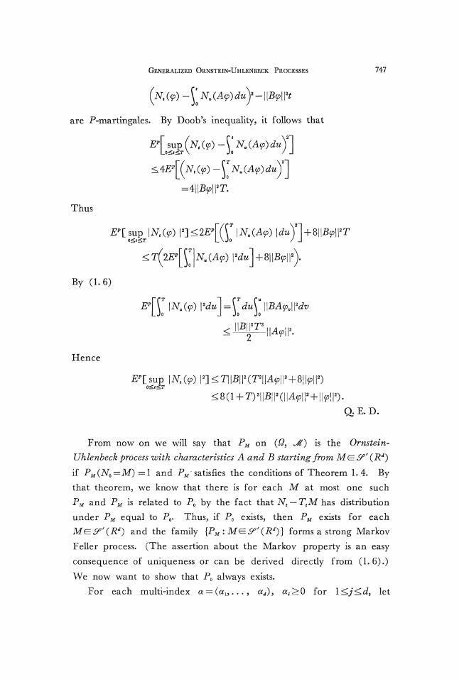
GENERALIZED ORNSTEIN-UHLENBECK PROCESSES 747
(AT, (?) - \' NU\ Jo
are P-martingales. By Doob's inequality, it follows that
Ep\ sup (Nt(<p)-{* Nu (A<p) duLo^^rX Jo /
Thus
By (1.6)
Hence
Q. E. D.
From now on we will say that PM on (Q, Jt} is the Ornstein-Uhlenbeck process with characteristics A and B starting from M^£f' (Rd)
if PM(JV0=M)=1 and PM satisfies the conditions of Theorem 1.4. Bythat theorem, we know that there is for each M at most one such
PM and PM is related to P0 by the fact that JV,-T,Mhas distributionunder PM equal to P0. Thus, if P0 exists, then PM exists for eachM<^<y'(Rd) and the family {PM:M^^'(Rd)} forms a strong MarkovFeller process. (The assertion about the Markov property is an easy
consequence of uniqueness or can be derived directly from (1.6).)
We now want to show that P0 always exists.For each multi-index a = (aly...9 ad)9 a,->0 for l<j<d, let

748 RICHARD A. HOLLEY AND DANIEL W. STROOCK
ha(x}=h, (X).../z,, (xd) where hk denotes the k'k Hermite function
(cf. A. 7). Given n>0, define #„: U(Rd~)->&(£*) by
(1. 10) nf9= Z (9, h,}ha!«!£»
It is weU-known that IIn<p-^(p as n-*oo 'm L2(Rd) for all <p^L2(Rd)
and that IIn(p->y in ^(Rd) for all <pE^<9*(Rd) (cf. A. 15).In order to carry out our construction we proceed as follows.
For n>0, set Dn = card{a: \a\<n} and define
(1.11) a..,=I r l
and
(1-12) b
for |a|, | /31 <n. Next let
(1. 13) L-" c\ L-i *~a,
It is easily shown that there exists on C([03 oo)5 RDn) exactly one
probability measure QM such that QM(y(0) =0) =1, EQU)[sup \y(f) |2]
<oo for all T>05 and f(y (t)) -{' LMf(y (5))ds is a QM-martingaleJo
for each f&C2b(R
Dn). (One can use, for example, Ito's stochasticdifferential equations as described in H. P. Mckean's [8].) Nextdefine t-^Nt^^'(Rd} by
(1. 14) Nt(9} = 2] (P, A.)y.(0, *>0 andui^»
Given a <p^ff>(Rd) and f<^C~(R1}, define
Note that
-ol.lfl^n
(V, ha)(
and

GENERALIZED ORNSTEIN-UHLENBECK PROCESSES 749
u|S J*.., (P, A.) (9, A,) = ^ E<n )rgM (Bh., Ar) (Bh,, Ar) (9, A.) (p, A,)
= E (Bnn(p,hry=\\nnBnn(p\\2.
Thus
1 ~2
+ (I] Jf, A.) ( g_6..^ (0)/' (#. (P)) •
But
L (P,A.) S6. lAy,(0= 2(2
From these calculations, we see that if Pw on (£?, Jf) is the distri-
bution of N. under Qw, then PW(N0=0)=1 and for all
and p
" (Ns (<p) ) ̂ — f (N,Z Jo
is a P('l)-martingale5 where
An=nnAHn and Bn=nnBIIn.
The next step is to show that {PM : n>Q] is weakly precompact.
To this end, note that because A is bounded from ^ (Rd) into itself,
there is an ra0>0 such that
(1.15)
for some C<\oo(cf. A. 18). For this m0, set n0 = m0-\-d + l and define
| |1- | | | on #"(Rd} by
(1.16)
It is easy to check that
(1.17) Xmt
is a complete separable Hilbert space under |||-||| and that the dual
of ffln can be identified in a natural way with the completion of
<? (Rd) under H H I l " 0 . Certainly it is enough for us to show that

750 RICHARD A. HOLLEY AND DANIEL W. STROOCK
P(n) is concentrated on C([0, oo), jf ) (which is an F,-subset of
C((0, oo), y" (£<))) for all n>Q and that {Pw : n>0} is weakly
precompact subset of probability measures on C([0, oo), j fB) . Since
under P(n) each N.(<p) is continuous and 2V. (AJ =0 a. s. for |a|>n, it
is clear that P(n) is concentrated on C([0, oo), j f B ) . Furthermore,
by (1.6)
for n>0, 0<^<^2, and <p^^(Rd). Thus, for any m>0, T>0, and
£>0:
lim sup P(w)( sup max |W( (Aa) -AT, (AJ | >e) =0.5^0 n O^t^t^T lal^m 2 !
'2- fl<3
Since PU) (NQ = 0) = 1 for all n>0, it only remains to check that for
T>0 and £>0 :
(1. 18) lim sup P(M)( sup |j|/7iWf|||>e) =0m-»oo n 0<.t<,T
where H^N is defined so that
But by (1.8) plus (1.15) :
and so
< L (2 a|+d)""ȣ'w[sup I^.CAJ

GENERALIZED ORNSTEIN-UHLENBECK PROCESSES 751
This proves that
lim sup EpW[sup|l!/7;^V,j|n=0m-»oo n Q<,t<T
which certainly implies (1. 18).
The final step in the construction is to show that if P is the limit
of a convergent subsequence {Pu/)} of {PU) : n>0} , then P(JVo = 0) =1,
Ep[sup \Nt(<p) |]<oo for all T>0 and <pSE^(Rd}, and0<,t<ZT
(1. 19) f(Nt(9))-\N,(A<p}f'(Nu(<p)}du-^^\f(Nu(<p)}duJo Z Jo
is a P-martingale for each f<=C™(Rd) and <p<E.y(Rd). But clearly
P(Aro=0)>TIrn P<»'>(N0 = 0)=1 and, by (1.8),
(1. 20) E"\_ sup |JV,(?>) ]2]<supEPll[ sup |tf,(fO 2]<oo.
Thus it only remains to prove that the expression in (1. 19) is a
P-martingale. Since the analogous expression, with An replacing A
and Bn replacing B, is a P^-martingale, it is easily seen that all we
must show is that
(1. 21) Ep[_Nt(A<p}F-] =HmEp(n''[Nt(An/riF]
for all £>0, <pE^^(Rd), and continnous P:C([0, oo), ̂ )->[- 1, 1].
But, by (1.6),
and clearly | |AM^— A^||->0 as n->oo. Thus proving (1.21) reduces
to showing that
(1. 22) Ep[Nt(A<p}F~] -lim Ep(n'\Nt(A^F~\.
However Nt(A(p)F is continuous, and therefore (1. 20) together with
the assumption that P(n/)->P implies (1.22). One final comment is
in order. We have just seen that {PU) : n>0] is precompact and
that every limit point satisfies P(N0=Q) =1 as well as the hypothesis of
Theorem (1.4). Thus by the uniqueness assertion in that theorem,
we conclude that P(n)-*P. We summarize our findings in the next

752 RICHARD A. HOLLEY AND DANIEL W. STROOCK
theorem.
(1. 23) Theorem : For each A and B there is a unique probability
measure P on (£?, ^) such that P(NQ=0) =1 and P satisfies thehypothesis of Theorem (1.4). Moreover, if An=IJnAIIn, Bn=nnBHn)
and P(n^ is the measure associated with An and Bn, then PM tendsweakly to P.
(1.24) Remark-. With very little alteration, the proof just givento get existence can be used to show that if An and Bn are generaloperators satisfying our basic hypothesis (not necessarily given byAn=nnAnn and En=UnEUn} and if there exists ra0>0 and C<oo
such that
then the measure PM associated with An and Bn tends to the P goingwith A and B if An-»A and Bn-*B strongly in L2(Rd).
§ 2. Branching Brownian Motion Having Finitely
Many Particles
In this section we recast the theory of branching Brownian motionin the setting of Levy processes. To be precise, let (Rd)(n} be definedfor n>\ to be the space of equivalence classes of 72-triples of
elements x^Rd mod permutations (i. e. (x1, . . . , ̂ ">=<y, . . . ,y> in(jRd) (n) if and only if there is a permutation a such that yk=xa(k\
\<k<d). Use n^ i (Rd)n-*(Rd)M to be the map taking (x\.. . ,xn)
into it's equivalence class in (Rd)M and topologize (Rd)M so that /7(n)
is open and continuous. Given a function/: (Rd)M->Rl, we say that/eC*((#')w)(C*((l?')^^
or C{((^)"))- Let E={$} U U (Rd)(n\ where 6 is an abstract point
and topologize E so that {0} as well as (Rd)M for each n>\ is bothopen and closed. Finally, let & (E) stand for the set of FiE-^R1
such that F restricted to (Rd)M is in C0°°((^)(n)) for all n>\ and

GENERALIZED ORNSTEIN-UHLENBECK PROCESSES 753
F = 0 on (Rd)M for all sufficiently large w's.
We are now nearly ready to describe the branching Brownian
motion with which we will be concerned. However, before doing so,
we need a little more notation. First, if F^C(E) has the property
that its restriction fn to (Rd)M is in C 2 ( ( R d ) M ) for all n>l , we
define JF(0) =0 and
where Ak stands for the Laplacian with respect to xk (notice that AF
is indeed well-defined on JE). Next, define for n>\ and \<k<n
<*\ . . . , *•>*€= (£<)(»+1) and <x\. . . ,*->4e (I?-)-1 (EE{^} ifn = l ) t obe, respectively, the element of E obtained by repeating or deleting xk.
With this convention we now define K on C(E) so that KF(<f>) =0
and for all n>l :
The branching Brownian motion which we want is the Levy process
on E having "diffusion part" determined by 1/2 A and "jump part"
governed by K. That is, <f> is absorbing and for n>\ the process
restricted to (Rd)M consists of n indepedent J-dimensional Brownian
motions, each of which waits a unit exponential holding time and then
with equal probabilities splits into two independent copies of itself
(moving the process to (^)(B+1)) or disappears (moving the process
to (fl')0"1')-For our purposes it is best to characterize the above process in
terms of a martingale problem. Let i2£=D([0, oo)3 E) be the space
of right continuous functions [0, oo) into E having left limits, and
endow @E with the usual Skorohod topology (this is possible since it
is clear that E admits a metrization in which it becomes a Polish
space). We will denote a generic element of E by rj and for w^QE
we will use r)(t, o>) to denote the position of a) at time £>0. For
£>0, set Jit = G(T](S) : Q<s<t) and observe that a ( \ J J [ t } coincides
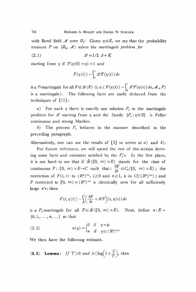
754 RICHARD A. HOLLEY AND DANIEL W. STROOCK
with Borel field Jt over QEm Given 5?e£, we say that the probability
measure P on (QE, ^) solves the martingale problem for
(2.1) J2? = l/2 A+K
starting from 37 if P(^(0) =37) =1 and
is a P-martingale for all F^ 3 (£) (i. e. ( F(i) (*) ) - J^F()? (5) ) <fc, uTf, P)Jo
is a martingale). The following facts are easily deduced from the
techniques of [11] :
a) For each j] there is exactly one solution P, to the martingale
problem for & starting from T] and the family [P^irj^E] is Feller
continuous and strong Markov.
6) The process P, behaves in the manner described in the
preceding paragraph.
Alternatively, one can use the results of [5] to arrive at a) and b).
For future reference, we will spend the rest of this section deriv-
ing some facts and estimates satisfied by the P/s. In the first place,
it is not hard to see that if S([0, oo) x£) stands for the class of
continuous F: [0, oo) xE-*C such that: <EC6([0, oo) xE) ; theot
restriction of F(t, •) to (U')w, t>0 and n>l, is in C!((-R')W) ; and
F restricted to [0, oo) x (^)Cn) is identically zero for all sufficientlylarge n's; then
is a P,-martingale for all Fe^([0, oo) x£). Next, define niE-
{0, 1,. . . , w,. . .} so that
0 if 3 = 0(2.2) *(?)= .,
m if
We then have the following estimate.
(2. 3) Lemma : // T>0 and ^<log( 1 +~ ),

GENERALIZED ORNSTEIN-UHLENBECK PROCESSES 755
Proo/: Set w(0 =1+ 2 -, 0<£<T, and, for m>l, define4 £(£ 1)
It is then clear that
°^* ro — <y p 0<9<T-^ xrt., USJS^ ,
so long as n(rj)<m. Hence
Fm(T-t/\T.,
is a P,-martingale, where
In particular,
j5;p,[^n(,(T))j <E\Fm(T-rm, ^(
i 2(g' — 1)
for all T>0 and /i>0 satisfying ^<logf 1 + ™ -. From this we see
/ 0 \that if ^</^<logf 1+^-J, then
and therefore {^w('(0) : 0<^<T} are uniformly P,-integrable. But this
means that we can let m t °° in the equality
and thereby arrive at (2.4) (since EP'|Vn(T)]<oo for some /!>0
certainly implies that rm | T (a. s., P,) as m->oo). Q. E. D.
One easy and important consequence of (2. 3) is the next theorem.

756 RICHARD A. HOLLEY AND DANIEL W. STROOCK
(2.5) Theorem: Let FeC([0, oo) xE) have the properties that
-T=—eC([0, oo) x£), F restricted to (Rd)(n} is in C2b((R
d')M) for eachot
n>l , and there is an M>0 and a C<oo such that
3F ,,, \D>F(t,ri\}<C n(rjr
for all t>0 and 5?e£, where D2F(t,<f>)=0 and for jye (U*)00, n>\
D2F denotes a generic second order spatial derivative of FoII(n\ Then
/(^^(O) "~\ \-^— + ̂ F)(sJ7](s)}ds is a P -martingale for allJo\ os J
(2. 6) Corollary : For all T>0 and ^<log( 1 +^
E '[ sup gin('(t-
/or a//
Proof: Take -F(^) =n(^) in the preceding theorem and concluded
that n(57(0) is a P,-martingale. Thus, if ^<logfl+|r\ then e^(fAT)
is a non-negative P,-submartingale. But this means (by Doob's
inequality) that
pEP'[sup
O^^T
where J</<log(l +|r. Q; E. D.
At this juncture we want to make a slight change in our point
of view. Namely, it is clear that E is homeomorphic to the set of
purely atomic integer-valued finite measures on Rd given the topology
of weak* convergence. That is, given r]EiE define for
(0 if v = <(2.7) ? (? )=<
As a consequence of (2.6), we see that for all <p(=B(Rd), T>0

GENERALIZED ORNSTEIN-UHLENBECK PROCESSES 757
(2.8) EP*[ sup eVf)]<oo,Q^t^T
where ^t((o) is the measure associated with ^(t, <x>) by the relation in
(2.7). We are now going to make exact computations of E '[^
and £
(2.9) Lemma: Set
(2. 10) ?t(x) = l /2 g-'*|2/2*, £>0 and
and for <p(=B(Rd) define
(2.11) <pt=r**<P-
(2. 12)
Moreover, if
(2. 13) £
Jw particular, if )7-
(2. 14) ^'[^(^l-W^^+ Cr,-.' (ft)1] (*)<&•
Proo/: We will assume that <p^C2b(R
d}. Given T>05 set
and
Since
it follows from (2.5) that F(t/\T, ij(t/\T)) and G(t/\T, y(t/\T))
are P,-martingales. Thus
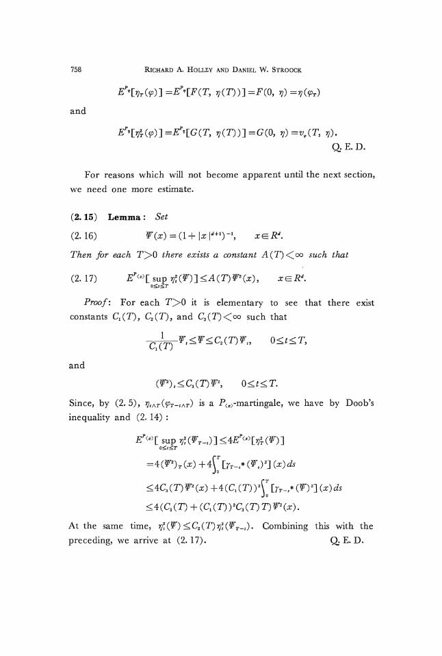
758 RICHARD A. HOLLEY AND DANIEL W. STROOCK
and
, ?(T))]=G(0, 7)=»f(T, 7).Q. E. D.
For reasons which will not become apparent until the next section,
we need one more estimate.
(2.15) Lemma: Set
(2. 16) W(x) =(l+\x I"1)-1, xeR1.
Then for each T>0 there exists a constant A(T)<oo such that
(2. 17) £P<3:>[sup
Proof: For each T^>0 it is elementary to see that there existconstants Q(T), C2(T), and C3(T)<oo such that
C(L ^<^<C2(T)f f, 0<t<T,
and
Since, by (2.5), ^Ar(^r-*Ar) is a P<x> -martingale, we have by Doob'sinequality and (2. 14) :
P<*1 supo^^r
<4C3 (T) F2 (j;) +4(C, (T)
At the same time, rft(W) <C2(T}rft(WT_t}. Combining this with the
preceding, we arrive at (2.17). Q. E. D.

GENERALIZED ORNSTEIN-UHLENBECK PROCESSES 759
§ 3. Branching Brownian Motion Having Infinitely
Many Particles
In this section we again discuss processes of the sort introduced
in section (2), only now we allow there to be infinitely many particles
initially. The approach that we adopt mimicks, for our setting, the
construction by Durrett [3].
For each x^Rd let QX=QE and ^x=^. Given a probability
space (£?, ̂ , P) on which there is an .Revalued point process ^
satisfying
(3.1) £
for bounded F^^Rd (\F\ denotes the Lebesgue measure of /"*), let
P=Px UP, on (Q, Jt}, where Q=Qx U Qx and J=Jx UJtf.
If w^Q, we let QJX, x^Rd, denote the xth coordinate of ft) and define
7r..(0) =37«(^«)-
(3-2) Lemma: Let W be the function in (2.16). Then for all
T>0:
(3.3) £*[£ sup %*e? o^t^r
In particular, if
(3.4) ft =
is a P-null set B^^ such that for all aJ&B the function
t-*fjt(<d) is right continuous and has left limits as a mapping from
[0, oo) into &"(Rd).
Proof: Suppose that (3. 3) has been proved. Then there is a
P-null set B<=^1 such that
converges uniformly on each bounded time interval for each
But if <p^Se(Rd), then \<p\<C,W for some C,<°°5 and therefore for

760 RICHARD A. HOLLEY AND DANIEL W. STROOCK
each &&B 2 fy.xfa ^) converges uniformly and absolutely on eachx<=$
bounded time interval. Since yt,x((p, #) is right continuous and has
left limits for all x(=Rd, <p^^(Rd), and a><=Q, we conclude that for
all co^B t-*r}t(a>) has the desired properties.
To prove (3.3), observe that by (2. 17) :
Thus, by (3. 1) :
Q.E.D.
Define *Mt for t>0 to be the a-algebra of subsets of & generated
by 9, (0>) for 0<s<£ and <p£=£f(Rd). The next theorem plays a
crucial role in our future results.
(3.5) Theorem: Given f^C2b(R
l) and
(3. 6)
w an (Q, J£t, P) -martingale.
Proof: What we must show is that if 0<t1<^t2 then
where
_ f ' / /(?. (y) + v (y) ) +/(g. (y) - p (y) )Jo H 2

GENERALIZED ORNSTEIN-UHLENBECK PROCESSES 761
and B is a set of the form
withn>l ;()<$!<. . .<5 W <^;^ , . . . ,^neE^(#«) ; and
Given ra>l, set
and define X (OT)(°) in terms of /, <p, and ^U). the same way as X(»)
is given in terms of /, 9, and 9. Then
where
and
Since (2. 5) applies to F, we know that
-0
for each d), and therefore we have now shown that
(XW(0, Jn P)
is a martingale. But, using (3. 3), it is easy to check that
as w-*oo in LX(P).
a- E. D.
We conclude this section with some preparations for the next two
sections. From now on we will be making the following assumption
about j] (in addition to (3. 1)) :

762 RICHARD A. HOLLEY AND DANIEL W. STROOCK
(3.7)
for some l<C<oo. Notice that both (3.1) and (3.7) are satisfied
by a Poisson random field. Also, observe that, in view of (3. 1),
(3.7) is an estimate on the variance of
(3. 8) Lemma : For all t>Q and
(3.9)
and
(3. 10)
Proof: To see (3.9), note that by (3. 1) and (2. 12) :
Next, by (2. 12) and (2. 14) :
SO

GENERALIZED ORNSTEIN-UHLENBECK PROCESSES 763
<(C+OIMI 2 . Q,E.D.
We next introduce a "central limit" type scaling of the process f).
Given #>0, we set
and define
(3. 12)
Observe that
(3.13)
and
That is:
(3. 14)
We next want to see what must be subtracted from /($"' (?0 ) to geta P-martingale. First observe that by (3.5) for /
- r' ^ ( r /(^(^(
is an (fl, ^2^5 -P) martingale. Since
and

764 RICHARD A. HOLLEY AND DANIEL W. STROOCK
we conclude that
,y-w+2)/2 rt
(?>W))— ̂ — \ ?,z, Jo a s
is an (<03 Ji 2t, P) martingale. Finally, because \A(jj(x}dx=Q for
all <p^y(Rd), we now have that for all f<=C2b(R
d) :
(3. 15)
.M (y) + PW ( • ) ) +/(^(g) (y) - yu)
is an (A ^_2j, P) martingale for all f^CKR1*) and co
Our final task in this section is to estimate Ep[ sup (^"'(p))2]- Too^jsr
this end first observe that (3. 14) together with (3. 15) shows that
is an (P, ^2 ? P) martingale. Thus, by Doob's inequality
£tr f ... r, .r /\ sup(7L 0<^T\
/2
and therefore :
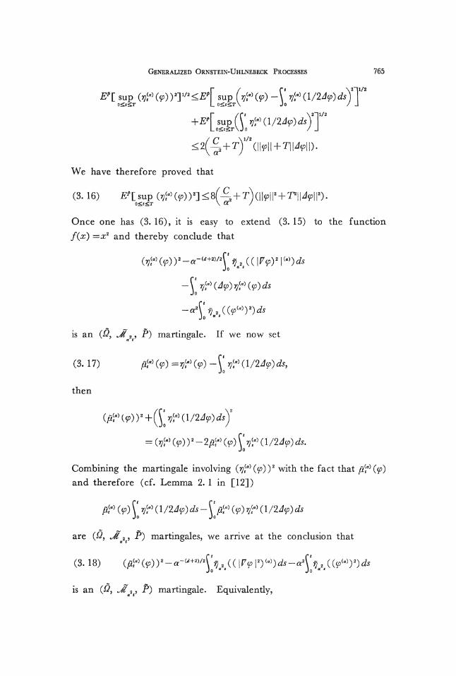
GENERALIZED ORNSTEIN-UHLNEBECK PROCESSES 765
sup W(9-)W<Ef\ sup
f /f* \2~|
sup(\ 7«(l/2^)&)Lo£t<£r\Jo / J
2~|l/2
1/2
We have therefore proved that
(3. 16) £?
Once one has (3. 16), it is easy to extend (3. 15) to the function
f ( x ) =xz and thereby conclude that
is an (Q9 JV 2> -P) martingale. If we now set
(3. 17) /2« (p) =7« (p)
then
Combining the martingale involving (^(a)(^))2 with the fact thatand therefore (cf. Lemma 2. 1 in [12])
are (Q9 Jt 2 , P) martingales, we arrive at the conclusion that
(3. 18) (/Z
is an (fi, ̂ 2 ? P) martingale. Equivalently,

766 RICHARD A. HOLLEY AND DANIEL W. STROOGK
(3.19) (/z^p))2-«-w+a)/a\V^Jo Jo
-a-*t\\\l79\\\*-t\\<p\\2
is an (Q9 ̂ av ^) martingale.
§4. Tightness of the Processes ^(a)
Let (O9 j?9 P), {^/t:t>Q}, and rf°\ be as in section (3) anddenote by P(tt) the distribution on D([0, oo), &' (Rd)} of ^(a). underP (cf. Lemma (3. 2)). What we are going to do in this section is showthat {P(tt) : a>l} is a tight (i.e. pre-compact) family, and then wewill show that for d>3 the limit lim P(a) exists and is the Ornstein-
«-»oo
Uhlenbeck process with characteristics 1/2^ and I. Although it is inconflict with the notation in section (1), we will use in this section Qto denote D([0, °o)3 &" (Rd)) and then define Nt, £>0; Jl ; and{Jtt : £>0} correspondly as in section (1) (only now for our newchoice of £). Finally, define the Hilbert space Jfd+3 with norm |||-|||as in (1. 16) and (1. 17) (i. e. take nQ=d + 3 in those equations). Thenext lemma shows that the P(fl° are concentrated on D([0, 00), Jt?d+3).
(4. 1) Lemma : // T>0 and a> 1, then
(4.2) ^U)[sup(Ar t(/i,))o^t^r
In particular, for all T>0 :
(4. 3)
(4. 4) lim sup £pG° [ sup 1 1 \H±Nt\ 1 12] - 0n-»oo «^i O^t^r
where Un is defined as in section (1).
Proof-. Clearly all that we have to do is prove (4.2). But (4.2)is an immediate consequence of (3. 16) plus the inequality (cf. A. 9)
Q.E.D.

GENERALIZED ORNSTEIN-UHLENBECK PROCESSES 767
In view of (4.4) we will have shown that {P(a) : a>l} is tight
and that any limit, as a->oo, lives on C([0, oo), jj?d+3) once we show
that for all n>l , £>0, and T>0 there is an a0 and a <5>0 for which:
(4.5) s u p P w ( s u p \\\nnNt-
Since IInN. is finite-dimensional, this reduces to studying each coor-
dinate N.(hp), \fi\<n, separately. Precisely what we need is proved
in the next lemma.
(4.6) Lemma: For all fl, s>0 and T>0 there is an aQ>l and a
d^>0 such that
(A 7\ SUP P^( sup \Nt(hp) — Ns(hp) i >s)<£.a^a° °^-1<^r
Proof: Given any right-continuous function /: [0, T]-*^1 having
left limits define
°^W<3"a-a^Vi50
( sup |/(0 -/(O) |) V( sup |/(T) -/(T-0 |)
and
^(«)= sup
Under the assumption that sup |/(^ + ) ~~/(^~) ^r? it is well-knownO^f^T
(cf. Parthasarathy [10] Lemma 6. 4) that wf(d) <2o)f(5) +r- Thus in
order to prove (4.7), all that we have to do is choose a0>l so that
JB)(#) |<e/2 whenever a>a0 and then show that
(4. 8) lim sup PM (ti.N(hft} (5) >s/4) =0.
The reason that this suffices is because one can easily show (cf. [11])
from (3. 15) that
(<p)-Nt_(& |<sup|f0wGr) | for allX
To prove (4. 8) we proceed as follows. By (3. 16) we can find

768 RICHARD A. HOLLEY AND DANIEL W. STROOCK
for each p^>0 an A<^oo such that
sup P«(sup (\Nt«£i o<Zt£T
Thus if
then P(a)(V<T)O for all a>\. Now define
Clearly, since p was arbitrary, (4. 8) will follow once we show that
(4. 9) lim sup Pw (0Z (<5) >s/4) -0.5-»0 a^l
Using Censov's criterion (cf. Theorem 15.6 in [!])> we will have
(4. 9) if we can prove that
sup £?w[(X(t3) -X(tJY(X(t2) -Xa)2]<52(^3-O2
«ai
for some B<^oo and all 0<^<^2<^<T. But we saw in section (3)
that (X(0, ̂ ,, -Pw) is a martingale; and, by (3. 19), it is clear that
is a supermartingale when 5 =.4 + 1+111^^1 If. Thus
Q. E. D.
We have now proved the next theorem (the details here, given
(4. 4) and (4. 5), are essentially the same as those given in preparation
for Theorem 1. 23)
(4.10) Theorem: The family {P(a) : a>\] is precompact on
£>([0, oo)? JfJ+3). Moreover, if aM-»oo and P=limP("") then P isn-»oo
concentrated on C([0, oo)3 jfJ+3) and therefore on C([0, oo)5 y'^))-

GENERALIZED ORNSTEIN-UHLENBECK PROCESSES 769
We are now ready to prove the main result of this section.
(4.11) Theorem: If d>3 then P(a)-*P as a-»oo where P is the
Ornstein-Uhlenbeck process with characteristics l/2d and I starting
from 0.
Proof: Because of Theorem (4. 10) and Theorem (1.4), it suffices
to show that if an->oo and P(%)-*Q, then Q(]V0=iO) =1, and for all
5 T>00£t£T
and
is a Q-martingale wheneverWe first note that Q(JV 0=0)=1 and that
sup^CjN.Cp) |]<°°3 T>0 and0£t£T
Indeed, each of these facts is an immediate consequence of (3. 14).Now let (p^^(Rd), /eQ0^1) and 0<^<^2 be given and suppose
that 0 : £)([0, oo)5 Jfd+3)-^[05 1] is a continuous J?t -measurable function.i
We must show that
(4. 12)
Let
Then, by (3. 15) :

770 RICHARD A. HOLLEY AND DANIEL W. STROOCK
i
where
Since sup £pU)[ sup (N,(^))2]<oo for all T>0 and ^e^(JZ'), ita£l OilfiT
is clear from the preceding that all we need do is show that (in the
notation of section (3)) :
(4. 13)
But, since /eCJ°(-Rrf), there is an A<oo such that :
where A=A s u i ^ ( ^ ) |. Thus
at a rate which is independent of 5. Thus we need only show that
as a-^oo3 uniformly on bounded ^-intervals. But to do this reduces to
proving
uniformly on bounded s-intervals. To this end, note that

GENERALIZED ORNSTEIN-UHLENBECK PROCESSES 771
and
Hence
and so, by (3. 14) :
11/2
We have therefore proved (4.13). Q. E. D.
The reader should remark that it is only in the derivation of(4. 13) that we have used the assumption that d>3. When d = 2one can proceed as follows. Denote by PU), a>l, the distributionunder P of f) 2 (^(a)). Observe that P(a) is concentrated on paths
as
with values in the space of "tempered measures" (i. e. non-negativeelements of ^'(P2)). One can then use the preceding to show that[Pa: «>1) is precompact and that any limit P as a-^-oo has theproperties that
P(iV0=Lebesgue measure) =1
and
(4. 14)
is a P-martingale for all <pe^(P2) and /eQ0^1)- G. Papanicolauhas pointed out to us that if [PN : N a tempered measure) is a familyof measures satisfying PN(NQ=N) =1 and (4.14) is a P^ martingalefor all ^e^(P2) and /eCr(P2) then it is the Markov family of

772 RICHARD A. HOLLEY AND DANIEL W. STROOCK
measures studied by Dawson in [2], [13], and [14], To see this let
g(t, x) solve the equation -^-=-^-^g — ̂ -g2 with g(Q, x)=<p(x)>Q.
Then setting f ( x ) =e~x in (4. 14) one sees that for all temperedmeasures N, exp[— Nt (g(T— t, - ))] is a P^ martingale for 0<t<T.(A careful proof of this uses critically the positivity of (p and henceof g(t, .) and Nt(g(T-t, • ))). Thus
This proves uniqueness of the solution to the martingale problem in(4. 14) and identifies the process.
Dawson [14] has shown that in 2 dimensions
for all £>0 and all (p with compact support. This corresponds to thesituation when d = 2 mentioned in the first paragraph of the introduc-tion.
If d = l, the Pws are again tight. Moreover Ep * [^(^)] =— ^W
and so any limit of the ^(a)'s must be concentrated at 0. ThusP(a^d0 as a f oo.
§ 5. Ergodic Theorems for Generalized Ornstein-Uhlenbeck Processses
In this section we consider O-U processes with characteristics Aand /. Throughout this section we assume that the semi-group, Tt
generated by A satisfies, in addition to the assumptions in Section 1,
the following :
(5. 1) p->\ \\Tt<p\\2dt is a continuous function onJo
Note that if there is a distribution R^&"(Rd) and
(5.2)
then (5.1) is satisfied. If A=~d and d>3 then (5.2) holds with
R(x) = constant/ | x\d~\ If A = -A2 and d>5 then (5.2) holds with

GENERALIZED ORNSTEIN-UHLENBECK PROCESSES 773
= constant/ \x \d~\ If A=A- \x \2 then
and so (5.1) holds (but not (5.2) since A—\x\2 is not translationinvariant.)
We rely heavily on the following fact :
(5.3) Levy Continuity Theorem (see [9]) : // {CB(0 \n>\} arecharacteristic functions of measures {/4;n>l} on <$?' (Rd) and foreach <p^^(Rd) Cn(^)— >C(^) where C(°) is continuous, then C is thecharacteristic function of a measure /j. and fjtn converges weakly to fj..
(5.4) Lemma: Let {PM : M^^(Rd)} be the O-U process withcharacteristics A and I. Then there is a probability measure /j, on^' (Rd) with characteristic function
and (JL satisfies
(5.5) \Pu(Nt^r)[t(dM)=n(.r) for all measurable rc#"(
(i.e., ft is stationary for [PM : Mey '(#*)})•
Proof: From Theorem (1. 4) (with Af = 0) we see that for all
is the characteristic function of a measure. Hence the existence offjt with characteristic function C follows from (5. 1) and (5.3). Tocheck (5. 5) it suffices to show that
(5.6)
But this follows immediately from Theorem (1.4). Q. E. D.
Now if f J t ^ ^ ' ( R d ) we define /*M to be ft shifted by M. Then

774 RICHARD A. HOLLEY AND DANIEL W. STROOGK
HM has characteristic function
Our next theorem shows that all stationary measures of the O-U
process with characteristics A and / must be a special kind of average
of the /*M5s.
(5. 7) Theorem : Let v be a stationary measure for the O-U process
with characteristics A and I. Then
(5.8) i>
where m satisfies
(5. 9) m(N^r) = m(TtN<=r)
for all £>0 and measurable rc^'(^).
Conversely any such measure m defines a stationary measure v by
(5. 8).
Proof: Suppose v is stationary. Then for all
(5. 10)
Hence \e** fV i>(d{jt), which is the characteristic function of a measure
»„ is equal to e*^''{f''(e™Vi>(dN). As t goes to infinity
(5. 11) \e^\ (dN) ^e*S~l[T*9{
which is continuous by (5. 1) ; and hence by (5. 3) is the characteristic
function of a measure m. Thus
(dM}

GENERALIZED ORNSTEIN-UHLENBECK PROCESSES 775
and therefore v = \fjtMm (dM) . Also
f iN(T «>) / 7 A T x T f *\ e 'ra ( rfJV) = lim \ eJ 5->00 J
- lim
which proves (5. 9) .
Conversely suppose (5.9) holds and define v by (5.8). Then
=̂ f g«(T|f)-i-/^V"a''-*/X^'
and so v is stationary. Q. E. D.
The next few lemmas are concerned with measures satisfying
(5.9).
(5.12) Lemma: If for all <p^^(Rd), Tt(<p)-*Q in & (Rd) as t^oo
then the only measure satisfying (5. 9) is the one concentrated on
zero. In this case, for all starting points M, PM°N~l converges weakly
to fji as t goes to infinity.
Proof: The first part of this lemma follows from (5. 3) and the
second part follows from (5.3) and Theorem (4. 1). Q. E. D.
(5.13) Example: If A=A— \x\2 then the hypotheses of Lemma
(5.12) are satisfied (see (A. 10) and (A. 15)).
(5. 14) Lemma : If m satisfies (5. 9) and is such that
m({N: there is an n such that AnN=Q}) =1
then m({N: TtN=N for all *})=!.
Proof: Using induction on (1. 1) one can easily show that for

776 RICHARD A. HOLLEY AND DANIEL W. STROOGK
all N^y'(Rd} and all
Thus if N is such that AnN=0 for some n, then N(Tt(p) -N(y>) as
a function of t is a polynomial with zero constant term. In particular
if N(Tt<p)±N(<p) for some t then \N(Tt<p) -N(<p) \ goes to infinity as
t goes to infinity. From this observation it is an easy exercise to show
that since N(Tt<p) and N(<p) have the same law under m for all t,
N(Tt<p) must equal N(<p) with m probability one. Since Tt(p is con-
tinuous in t and (p separately and [0, oo) and y (Rd) are separable,
it follows that
m(N=TtN for allQ. E. D.
We want to show that the hypotheses of Lemma (5. 14) are
satisfied by A =-~-4 but first we need the following result about tem-
pered distributions.
(5. 15) Lemma : Let ffE=C°°(Rd) and assume that a and its derivatives
grow no faster than polynomials. Let N be a tempered distribution
with support S and assume that Sd{x:a(x} = 0}. Then there is an
integer m such that amN = 0.
Proof: Suppose first that S is compact. Then AT is a distribution
with compact support and hence there is a number C>0 and an
integer n such that for all (p
(5.16) \N(<p)\<Clal^n y
We take m=n + l and show that amN=Q.
Let p$E:C~(Rd) with support in [x : \x \ <!}, ^>0 and (p(x)dx = l.
Define ps (x) =e~dp(—} and ^s (x) =p.*I 2e, where 5e = [x : dist (x, S) <e] .\ e / s
Note that <p<(x) =1 if x^S* and thus, since supp amNdS, </>eamN=amN.
Next note that \Da<f>.(y) | <e~ | a l\ \Dtp(x) \dx and that sup \o*(x)\ isJ xGS36
bounded by a constant times ey. Thus if 0<^s<l and \a\<^m, then

GENERALIZED ORNSTEIN-UHLENBECK PROCESSES 777
sup \Daam(x} | is bounded by a constant times sm~ | a l. Since <J)t(x) =0*eS3e
if x^S3e it follows easily that sup | Da$s(jm (y ) is bounded by a
y _
constant times eTO~ Ia |. Thus there is a constant C such that for all
0<e<l
<p) I <C 2 sup |
that is, amN=Q.
If *S is not compact let ?n^C~ be such that
1 ifr 3; =
10 if
Then ynN has compact support and satisfies the hypotheses of the
lemma. Thus by the above there is an m, which depends only on
the order of N, such that j-namN = 0. (Here we rely on the assump-
tion that N is tempered.) In particular the support of 0mN does not
intersect [x : \x\<n}. Since this is true for all n, amN=0.
Q. E. D.
We want to apply the above lemma to the following situation.
Suppose 0^C°°(Rd), 0<Q} a(x)=a(—x),> and a and its derivatives
grow no faster than polynomials. If <p^,9yc(R
d) let 0 denote its/\
Fourier transform. Define an operator A on £fc(Rd) by A<p=a<p,
Since 0"<0 A is non-positive definite; and, since a(x)=a(—x), A<p
is real valued if <p is real valued. A generates a self -adjoint semi-/\
group, T0 given by Tt<p=eta(p.
If AT is a tempered distribution N (<p) = N (iff) .
(5. 17) Lemma : Let A and Tt be as above and let m be a probability
measure on <?' ' (Rd) satisfying (5.9). Then
m(T,N=N for all 0=1-
Proof: By Lemma (5. 14) it suffices to show that
(5. 18) m([N: there is an m such that AmN = 0} ) = 1 .

778 RICHARD A. HOLLEY AND DANIEL W. STROOCK
But 'A"*N=amN, and thus by Lemma (5. 15), (5. 18) will follow if
we can show that
(5. 19) m({N: supp #czeros of <?}) =1.
To see (5. 19) let <p<=3*c(Rd) be such that support £?n [x : o(x} =$} = <f>.
Then as t goes to infinity eat<p converges to 0 in £fc(Rd). Now since
for all £>0 the laws under m of N and TtN are the same, it follows
that the laws of N and TtN are the same. Hence N(<p) and
T\N((p)=N(eta(p} have the same law for all t>0. But #(*"p)-*0
as t-*oo for all N^9"(Rd). (5. 14) foUows easily from this.
Q. E. D.
(5.20) Example: If A=-L/ and a(x) = -y \x |2, then A and a
are related as in Lemma (5. 17). Thus it follows from Lemmas (5. 17)
and (5. 7) that all stationary measures for the O-U process with
characteristics -^-J and I are convex combinations of {{JLH ' H a har-
monic function in £?'(Rd)}. It is also easy to see that the //H are
the extreme points of the set of stationary measures.If v is a stationary measure given by (5. 8) with m satisfying
(5. 9), then whether or not u makes the process time reversible seems
to be closely related to whether or not m satisfies
(5.21) m({N: TtN=N})=l
for all £>0. One direction of this relation is made clear by the
following lemma.
(5. 22) Lemma : // v is given by (5. 8) and m satisfies (5. 21) then
v makes the process time reversible^ i. e.5 for all 0<s<^t and <p,
(5. 23)
Proof: By making use of Theorem (1.4) it is a straightforward
computation to check that

GENERALIZED ORNSTEIN-UHLENBEGK PROCESSES 779
r w(f.+v-*JoM|^||2rf«-*/^^
and
r oo TOO
Since Tf is self -adjoint \ (^tt, ^_s+u)<^ = \ (^_^M3 $u)du. If m
satisfies (5. 21) then M(&)°=M (0) and M (p,°) =M(p) for all £ and
s(a. 5. ra). and we have the desired result. Q. E. D.
(5. 24) Remark : From the proof of Lemma (5. 22) we see that
the condition on m that is equivalent to \> being time reversible is
that for all 0<s<£ and all p, <p^ff>(Rd), the law of (Af(p,), M(&))under m is the same as the law of (M(<^)5 M(^,)) under m. Clearly
(5. 21) implies this, but we are unable to decide if the oppositeimplication holds.
The final goal of this section is to find a Banach space (X, ||-||z)contained (topologically) in &*' (Rd) such that: i) X is a dense Fff in
£f'(Rd) ; ii) for each MeX the O.-U. process PM with characteristics
-^A and I starting from M is concentrated on C([0, oo), X) ; and
iii) for each MeX and all $eC6(X), £ M [ ^ ( A T J ] - > ^ 0 as
where //0 is the probability measure on &' (Rd) with characteristic
function
[—^exp
Observe that if we prove iii), then automatically /^0(X) =1. Moreover,
we will have shown that X is a state space for the (Feller continuous)
Markov family [PM : MeX} and that [PM : MeX] is ergodic with
fjtQ as its unique stationary measure. (The Feller continuity is irrele-
vant for these considerations but will follow from our estimates below
plus the uniqueness which we have already proved in Theorem

780 RICHARD A. HOLLEY AND DANIEL W. STROOCK
(1. 4)).
In view of our characterization of the stationary measures for
{PM: M<=y'(jRJ)h it is clear that what has to be done is find aBanach subspace X of &" (Rd) such that 7-,*Af-»0 strongly as £-»oo
for all M^X. At the same time, this subspace must be chosen sothat P0 is concentrated on C([0, oo)3 X) and in addition that t->yt*M
is strongly continuous into X for all M^X (this latter condition isneeded in order to assure that PM is also concentrated on C([0, oo),X)). Finally, X must have the property that the one-dimensionaltime marginals P^N^1 of P0 are tight. Considering all the conditionsthat must be met, it is somewhat surprising that X is so easy to describe.
Given p>0 and w>0, define ||-||(,.»> on ff" (Rd) by
and let X(p,m, = {N^ff"(R*} : ||N||(,..)<oo}. (See (A. 19) for the
definition cf | l | - | | l ( » )« ) It is easy to see that each X(,I|B) is a dense Fa
in &"(Rd) (density comes from the inclusion C%(Rd)<^X^tm^ and
that (X(pifB), | | - | l ( p , m ) ) is a Banach space.
(5.25) Lemma: For all M^.X(pifn^ t-*ft*N is strongly continuous
on [0, oo ) into X(/,iJB) and ll^*2V|| ( />fW)->0 as t-*oo. Moreover, for all
Q<^p<^a and w>0, bounded closed subsets of X(0im^ are compact as
subsets of X(,iBI+1).
Proof: Since rt+t=rt*T*9 we need only check that t-*7t*N iscontinuous from [0, 1) into X(/,tm). To this end, note that by (A. 23) :
and
supll lr^rQ£t£l
Thus, in order to prove that
]im\\rt*N-r,*N\\<,.*=Ut-*sf£Q
for WeX(/,§m) and 5e[0, 1), it suffices to show that

GENERALIZED ORNSTEIN-UHLENBECK PROCESSES 781
When s>0, this is obvious from (A. 24). When 5=0, we argue as
follows. Since N^X(pim^ it is clear that Yi/n*N-*N in X(,I|B) as n->oo00
because 2 ra'lll7'i/.*-N— Nl'lw^00- Thus if s>0 and we choose n, so
that 2C./».<« and |||ri/.*Mr--N'lllw<e for n>n,, then, by (A. 24),
for all te.\ - — . — where n>n, :L n+l nj
\\\r,*N-N\\\M<\\\rt*N-ri,a*N\\\w+e
The proof that \\Tt*N\\(pim)-*Q as t-*oo for N^X(pim^ is an easy
consequence of the definition of X(ptm^ together with (A. 23). Finally,
the assertion that bounded subsets of X(ffim^ are compact subsets of
X(p>OT+1) is proved in exactly the same way as one shows that a bound-
ed self-adjoint operator is compact if it has a completely discrete
spectrum having zero as its only accumulation point. Q. E. D.
(5.26) Lemma: For all 0<io<l/2 and m>rf + 6 the measure PQ is
concentrated on C([0. oo), X (p>m)) and
(5.27)<SO
Proof: First note that for 0<s<£
and that if X is a normal random variable with mean zero, then
E[X6]=15(E[X2])3. Thus
(5.28) E
Applying (5. 28) to f,-i*<p we have

782 RICHARD A. HOLLEY AND DANIEL W. STROOCK
Also
and for n>2 :
Using (A. 11) and (A. 12) together with the above, we get:
(5. 29) E\% n'||!r.-,*JV1-r.-l«N.|||«w]^A..,.,(«-*)'n = l
and
(5. 30) £P°[Z n'HIr.-.-N.IH?.,] <Bm,d,fn = l
for some Amidi? and Bm.rf,p so long as m^>d + 6 and
Next, from (5. 28) we have
Also, taking s=Q;
2 \ 3
du
2
du
Since, by (A. 14), \\Aha\\*<dC(Q, 2)(2|«|+^)2, we can use the pre-
ceding to find Cm:dif and Dm:dif such that
(5.31) ^e[f:
and
(5. 32) £P°[i;

GENERALIZED ORNSTEIN-UHLENBECK PROCESSES 783
for all 0<><l/2 and m>d+6.
Combining (5.29) and (5.30), we arrive at
(5. 33) E
which implies that P0(C([0. oo), X (,, t JB)))=l (since we already know
that t-+Nt(<p) is continuous for all ^e^(^))- Finally, (5.30) and
(5.31) yield:
Q. E. D.
We now have all the necessary facts to complete our program. Let
and 0<10<l/2 be given. By the preceding we know that
oo)3 X ( j B i m ) ) )=l . Since for every MeX(,>BO PM coincides
with the distribution of ft*M+Nt under P0, it follows from Lemma
(5.25) that PM(C([0, oo)5 X(,. „)))=! and that for any @<=Cb(X(pim^
=0.
Finally, by Lemmas (5. 25) and (5. 26) we know that the measures
{P0oN~l: t>0} are pre-compact on X(/,>m) and we have already seen
that P0°N~l-*/ji0 on &"(Rd} ; and therefore jPjfOJVr1-*/^ on X(pim^ for
all M"eX(p>m). With these remarks we have now proved our final
theorem.
(5.34) Theorem: If m>d + 7 and 0<><l/2, then the collection
[PM : M^X(pim^} forms a strong Markov, Feller continuous family on
C([0, oo), X(,.m)) and
for all
Appendix
The purpose of this appendix is to catalogue some facts about
Hermite functions. We do not pretend that these facts are unknown,

784 RICHARD A. HOLLEY AND DANIEL W. STROOCK
in fact many of them have become part of the standard folklore
among experts in distribution theory. All that we want to do is
compile them here for the convenience of our readers.
Given k>0, define gh: Rl-*Rl by
(A.I) gk(x)=(-iye*'*Die-*\
An obvious and basic fact is that
(A. 2) E-£-g*(x) =e-*2/*+2**-*\ x^R1 ando k\
From (A. 2) it is not hard to derive :
(A. 3) xgk (*) =±gk+l (x) +kgk_1 (x)
and
(A. 4) &(x) =kgk_l(x) -
where #_! = (). Combining (A. 3) and (A. 4), one can easily arrive
at
(A. 5)
Starting once again with (A. 2), one sees that
rO if(A. 6)
Thus if
(A. 7)
then {hk: k>0} forms an orthonormal sequence in L2(R^. The
function hk is called the kth Hermite function. A well-known fact is
that {hk: k>0} is a basis in U(R1}. From (A. 3), (A. 4) and (A. 5),
we obtain:
(A. 8) xht(x)
(A. 9) h\(x)

GENERALIZED ORNSTEIN-UHLENBECK PROCESSES 785
and
(A. 10) (-D2x+x2)hkW=
Another consequence of (A. 2) is
(A. 11) hk=ikhk, k>0,
where
Thus, by the Fourier inversion formula and (A. 8) :
1/2
for each e>0. Taking £1/2 = (2& + l)1/4, we arrive at:
(A. 1 2) i hk O) | < C-?- Y/2 (2k + 1 ) 1/4, A > 0 and x e ^'.\ 7T /
Next define for «e({0, 1, . . . , ^,...}) i the function h, : Rd^R"
by
(A. 1 3) hm (x) = h« (xj ...h. (xd) , x<=Rd.1 d
Properties of the ha's art easily read off from the correspondingproperties of the hk's. In particular, from (A. 8) and (A. 9), we can
use induction to show that for all //, ye({0, 1 , . . . ,k,...})d there isa C((JL, v) such that
(A. 14) \\x*D:ha\f<C(& p ) (2 | a |+d )W + M .
Also, if <p^<Sf(Rd), then integration by parts shows that {(^?, Aa) :
a:>0} is rapidly decreasing (i.e. |a|"|(^, htt) |— >0 as | a | — >oo for all
n>0). Thus if 9?e^(-R r f), then from (A. 14) we have:
\\x'DX<p- Z C ^ A J A J I I ^ E l(pA)|

786 RICHARD A. HOLLEY AND DANIEL W. STROOGK
as 2V t °°. In other words:
(A. 15) E (MJ^— ? in ST(Rd)\a\£N
for all <p^<9y(Rd). In particular, we can again use (A. 8) and (A. 9)
to show the existence of K([JL, i/) such that
(A. 16) \\x«D:9\\2<K([jt, i,) E (2 k I
for all <p<^y (Rd). In view of (A. 10) and (A. 16), we come to the
important conclusion that for each m>0 there exist
such that
(A. 17)
where
(A. 18)a
We now want to derive some slightly less standard facts about
&"(Rd}. Namely, let
(A. 19)
It is obvious that 3? (OT) is a complete separable Hilbert space. In fact
Jf(m) can be identified as the dual of the completion Jf(OT) of Sf (Rd)
with respect to iHIU ) (for this identification one uses (A. 15)) ; and
the action of JV(Ejf(m) on JfU) is given by:
(A. 20)
Of course, if (p^^(Rd} then N(p) given by (A. 20) coincides with
the action of A^ as an element of Sf* (Rd} on <p (this fact justifies
our use of the notation N(<p) in (A. 20).) Asa consequence of these
considerations we see that
(A. 21) |||tf|||w= sup
We are at last ready to prove the next estimate.
(A. 22) Theorem : Define r.*N, ^>0 and N^^f(Rd}, by -{t*N(<p) =
N(r,*<p)- Then for all m>® and T>0 there is a COT(T)<oo such
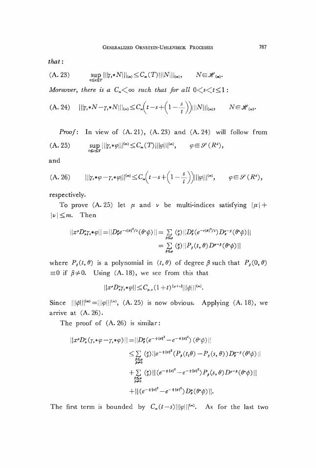
GENERALIZED ORNSTEIN-UHLENBECK PROCESSES 787
that:
(A. 23) sup \\\rt*N\\\M<Cm(TmN\\\M,O^t^T
Moreover, there is a Cm<^oo such that for all
(A. 24) l!!n*^-
Proof: In view of (A. 21), (A. 23) and (A. 24) will follow from
(A.25) sup | i [0<£*£T
and
(A. 26) ||lr,^
respectively.
To prove (A.25) let ^ and v be multi-indices satisfying \fi\
\v\<m. Then
where Pp(t,0) is a polynomial in (t,0) of degree (3 such that
= 0 if j8^=0. Using (A. 18), we see from this that
Since |||^l||(")=ilMH("), (A.25) is now obvious. Applying (A. 18), we
arrive at (A. 26) .
The proof of (A. 26) is similar :
<£ OD»<.?f-t-o
The first term is bounded by Cw(it—5)|||p|||('"). As for the last two

788 RICHARD A. HOLLEY AND DANIEL W. STROOCK
terms, note that \e~~fl(?|2 — e~'fm | achieves its maximum at any
such that se * °°l =te + *0' . Thus
«" - - tHence the last two terms are bounded by
Applying (A. 17) we arrive at (A. 26).
References
[ 1 ] Billingsley, P., Convergence of Probability Measures, New York: John Wiley and Sons(1968).
[ 2 ] Dawson, D., and Ivanoff, G.5 Branching Diffusions and Random Measures, to appear.[ 3 ] Durrett, R., An infinite particle system with additive interactions, to appear.[ 4 ] Fleischman, J., Limiting distributions for branching random fields, to appear Trans.
Amer.Math. Soc.[ 5 ] Ikeda, N., Nagasawa, M., and Watanabe, S., Branching Markov processes I, II, and
III, J.Math. Kyoto Univ.,8 (1968), 233-278, 365-410, 9 (1969), 95-110.[ 6 ] Kallenberg, O., Stability of critical cluster fields, to appear.[ 7 ] Martin-Lof, A. Limit theorems for motion of a Pousson system of independent Mar-
kovian particles with high density, Z. Wahr. Verw.Geb.,U (1976) 205-223.[8] McKean, H. P., Stochastic Integrals, New York: Academic Press (1969).[9] Meyer, P. A., Le Theoreme de Continuite de P. Levy sur les Espaces Nucleairs. Sem.
Bourbaki, 18 e annee, 1965/66 no. 311.[10] Parthasarathy, K. R., Probability Measures on Metric Space, New York: Academic
Press (1969).[11] Stroock, D.W., Diffusion processes associated with Levy generators, Z. Wahr. Verw.
Geb.,B2 (1975), 209-244.[12] Stroock, D.W. and Varadhan, S. R. S., Diffusion processes with boundary conditions,
Comm.Pure. Appl.Math.,24 (1971) 147-225.[13] Dawson, D., Stochastic Evolution Equations and Related Measure Processes, J. Multi-
variate Anal.,5 (1975), 1-52.[14] Dawson, D., The Critical Measure Diffusion Process, to appear.