Generating Compiler Optimizations from Proofs ∗

Ross Tate Michael Stepp Sorin LernerUniversity of California, San Diego{rtate,mstepp,lerner}@cs.ucsd.edu

AbstractWe present an automated technique for generating compiler op-timizations from examples of concrete programs before and afterimprovements have been made to them. The key technical insightof our technique is that a proof of equivalence between the originaland transformed concrete programs informs us which aspects of theprograms are important and which can be discarded. Our techniquetherefore uses these proofs, which can be produced by translationvalidation or a proof-carrying compiler, as a guide to generalizethe original and transformed programs into broadly applicable op-timization rules.

We present a category-theoretic formalization of our proof gen-eralization technique. This abstraction makes our technique appli-cable to logics besides our own. In particular, we demonstrate howour technique can also be used to learn query optimizations for re-lational databases or to aid programmers in debugging type errors.

Finally, we show experimentally that our technique enables pro-grammers to train a compiler with application-specific optimiza-tions by providing concrete examples of original programs and thedesired transformed programs. We also show how it enables a com-piler to learn efficient-to-run optimizations from expensive-to-runsuper-optimizers.

Categories and Subject Descriptors D.3.4 [Programming Lan-guages]: Processors – Compilers; Optimization

General Terms Languages, Performance, Theory

1. IntroductionCompilers are one of the core tools that developers rely upon, andas a result they are expected to be reliable and provide good perfor-mance. Developing good compilers however is difficult, and the op-timization phase of the compiler is one of the trickiest to develop.Compiler writers must develop complex transformations that arecorrect, do not have unexpected interactions, and provide good per-formance, a task that is made all the more difficult given the numberof possible transformations and their possible interactions.

The broad focus of our recent work in this space has beento provide tools that help programmers with the difficulties ofwriting compiler optimizations. In this context, we have done workon automatically proving correctness of transformation rules, on

∗ This work was supported by NSF CAREER grant CCF-0644306.

Permission to make digital or hard copies of all or part of this work for personal orclassroom use is granted without fee provided that copies are not made or distributedfor profit or commercial advantage and that copies bear this notice and the full citationon the first page. To copy otherwise, to republish, to post on servers or to redistributeto lists, requires prior specific permission and/or a fee.POPL’10, January 17–23, 2010, Madrid, Spain.Copyright c© 2010 ACM 978-1-60558-479-9/10/01. . . $5.00

generating provably correct dataflow analyses, and on mitigatingthe complexity of how transformation rules interact.

Despite all these advances, programmers who wish to imple-ment optimizations often still have to write down the transforma-tion rules that make up the optimizations in the first place. This taskis error prone and tedious, often requiring multiple iterations to getthe rules to be correct. It also often involves languages and inter-faces that are not familiar to the programmer: either a language forrewrite rules that the programmer needs to become familiar with,or an interface in the compiler that the programmer needs to learn.These difficulties raise the barrier to entry for non-compiler-expertswho wish to customize their compiler.

In this paper, we present a new paradigm for expressing com-piler optimizations that drastically reduces the burden on the pro-grammer. To implement an optimization in our approach, all theprogrammer needs to do is provide a simple concrete example ofwhat the optimization looks like. Such an optimization instanceconsists of some original program and the corresponding trans-formed program. From this concrete optimization instance, our sys-tem abstracts away inessential details and learns a general opti-mization rule that can be applied more broadly than on the givenconcrete examples and yet is still guaranteed to be correct. In otherwords, our system generalizes optimization instances into correctoptimization rules.

Our approach reduces the burden on the programmer whowishes to implement optimizations because optimization instancesare much easier to develop than optimization rules. There is nomore need for the programmer to learn a new language or inter-face for expressing transformations. Instead, the programmer cansimply write down examples of the optimizations that they want tosee happen, and our system can generate optimization rules fromthese examples. The simplicity of this paradigm would even enableend-user programmers, who are not compiler experts, to extend thecompiler using what is most familiar to them, namely the sourcelanguage they program in. In particular, if an end-user programmersees that a program is not compiled as they wish, they can simplywrite down the desired transformed program, and from this con-crete instance our approach can learn a general optimization rule toincorporate into the compiler. Furthermore, optimization instancescan also be found by simply running a set of existing benchmarksthrough some existing compiler, thus allowing a programmer toharvest optimization capabilities from several existing compilers.

The key technical challenge in generalizing an optimizationinstance into an optimization rule is that we need to determinewhich parts of the programs in the optimization instance mattered,and how they mattered. Consider for example the very simpleconcrete optimization instance x+(x-x) �⇒ x, in which the variablex is used three times in the original program. This optimizationhowever does not depend on all three uses referring to the samevariable x. All that is required is that the uses in (x-x) refer tothe same variable, whereas the first use of x can refer to anothervariable, or more broadly, to an entire expression.

Our insight is that a proof of correctness for the optimizationinstance can tell us precisely what conditions are necessary for theoptimization to apply correctly. This proof could either be gener-ated by a compiler (if the optimization instance was generated froma proof-generating compiler), or more realistically, it can be gener-ated by performing translation validation on the optimization in-stance. Since the proof of correctness of the optimization instancecaptures precisely what parts of the programs mattered for correct-ness, it can be used as a guide for generalizing the instance. Inparticular, while keeping the structure of the proof unchanged, wesimultaneously generalize the concrete optimization instance andits proof of correctness to get a generalized transformation and aproof that the generalized transformation is correct. In the exampleabove, the proof of correctness for x+(x-x) �⇒ x does not rely onthe first use of x referring to the same variable as the other uses in(x-x), and so the optimization rule we would generate from theproof would not require them to be the same. In this way we cangeneralize concrete instances into optimization rules that apply insimilar, but not identical, situations while still being correct.

Our contributions can therefore be summarized as follows:

• We present a technique for generating optimization rules fromoptimization instances by generalizing proofs of correctnessand the objects that these proofs manipulate (Section 2).• We formalize our technique as a category-theoretic framework

that can be instantiated in various ways by defining a few keycategories and operations on them (Section 3). The general na-ture of our formalism makes our technique broadly applicable.• We illustrate the generality of our framework by instantiating

it not only to compiler optimizations (Section 4), but to otherdomains (Section 5). In the database domain, we show thatproof generalization can be used to learn efficient query opti-mizations. In the type-inference domain, we show that proofgeneralization can be used to improve type-error messages.• We used an implementation of our approach in the Peggy com-

piler infrastructure [22] to validate the following three hypothe-ses about our approach: (1) our approach can learn complex op-timizations not performed by gcc -O3 from simple examplesprovided by the programmer (2) it can learn optimizations fromPeggy’s expensive super-optimization phase (3) it can learn op-timizations that are useful on code that it was not trained on.

2. OverviewThe goal that we are trying to achieve is to generalize optimizationinstances into optimization rules. The key to our approach is touse a proof of correctness of the optimization instance as a guidefor generalization. The proof of correctness tells us precisely whatparts of the program mattered and how, so that we can generalizethem in a way that retains the validity of the proof structure.

Intuitively, our approach is to fix the proof structure, and thentry to find the most general optimization rule that a proof of thatstructure proves correct. Focusing on a given proof structure alsohas the added advantage that, once the structure is fixed, we will beable to show that there exists a unique most general optimizationrule that can be inferred from the proof structure, something thatdoes not hold in general. For example, consider the optimizationinstance 0 ∗ 0 �⇒ 0. This transformation has two incomparablegeneralizations, X ∗ 0 �⇒ 0 and 0 ∗ X �⇒ 0, depending on whetherone uses the axiom ∀x.x∗0 = 0 or ∀x.0∗x = 0 to prove correctness.However, once we settle on a given proof of correctness, not onlydoes there exists a most general optimization rule given the proofstructure, but we can also show that our algorithm infers it.

In this section, we start by giving some examples of proof-basedgeneralization (Section 2.1), explain some of the challenges be-

hind generalization (Section 2.2), give an overview of our technique(Section 2.3), and finally describe a way of decomposing optimiza-tions we generate into smaller independent ones (Section 2.4).

2.1 Generalization examplesFigure 1 shows an example of how our approach works. We de-scribe the process at a high-level, and then describe the details ofeach step. At a high-level, we start with two concrete programs,presenting an example of what the desired transformation shoulddo – parts (a) and (b); we convert these programs into our own in-termediate representation – parts (c) and (d); we then prove that thetwo programs are equivalent, a process known as translation vali-dation – part (e); from the proof of equivalence we then generalizeinto optimization rules – parts (f) and (g) show two possible gener-alizations. We now go through each of these steps in detail.

The optimization that is illustrated in parts (a) and (b) of Fig-ure 1 is called loop-induction variable strength reduction (LIVSR).The optimization essentially replaces a multiplcation with an addi-tion inside of a loop.

As we will show in Section 3, our approach is general and canbe applied to many kinds of intermediate representations, and evento domains other than compiler optimizations. However, to makethings concrete for our examples, we will use the PEG and E-PEG intermediate representations from our previous work on thePeggy compiler [22] (this is also the representation we use in ourimplementation and evaluation).

Part (c) of Figure 1 shows a Program Expression Graph (PEG)representing the use of i*5 in the code of part (a). A PEG containsnodes representing operators (for example “+” and “∗”), and edgesrepresenting which nodes are arguments to which other nodes. Thearguments to a node are displayed below the node. The top of thePEG contains a multiply node representing the multiply from i*5.The θ node represents the value of i inside the loop. In particular,the θ node states that the initial value of i (the left child of θ) is 0,and that the next value of i (the right child of θ) is 1 plus the currentvalue of i. Similarly, part (d) of the figure shows the PEG for theuse of i in part (b).

Now that we have represented the two programs in our interme-diate reprensentation, we must prove that they are equivalent. Wedo so using an E-PEG, which is a PEG augmented with equalityinformation between nodes. Graphically, we represent two nodesbeing equal with a dotted edge between then, although in our imple-mentation we represent equality by storing the equivalence classesof nodes. Part (e) of Figure 1 is an E-PEG, constructed by apply-ing four equality axioms to the original PEG: edge a© is added byapplying the axiom θ(x, y) ∗ z = θ(x ∗ z, y ∗ z); edge b© is added byapplying the axiom (x + y) ∗ z = x ∗ z + y ∗ z; edge c© is added byapplying the axiom 1 ∗ x = x; and edge d© is added by applyingthe axiom 0∗ x = 0. This E-PEG represents many different versionsof the original program, depending on how we choose to computeeach equivalence class. By picking θ to compute the {∗, θ} equiva-lence class, and + to compute the {∗,+} equivalence class, we getthe PEG from Figure 1(d), and as a result, the E-PEG thereforeshows that the PEGs from parts (c) and (d) are equivalent.

In our Peggy compiler, there are two ways of arriving at theE-PEG in Figure 1(d). The first is as described above: we converttwo programs into PEGs and then repeatedly add equalities untilthe result of the two programs become equal. The other approachis to start with just an original program and PEG, say the onesfrom Figure 1(a) and 1(c), and construct an E-PEG by repeatedlyapplying axioms to infer equalities. A profitability heuristic canthen select which PEG is the most efficient way of computing theresults in the E-PEG, which in our case would be the PEG fromFigure 1(d).

θ+0

1

*

5

θ+0

5

i := 0while(...){use(i)i := i+5

}

i := 0while(...){use(i*5)i := i+1

}

θ+0

1

* θ

*5

+*0 5

05*

1 55

a

c

d b

(b)

(a)

(d)

(c)

θ+0

1

*

Cθ

+0C

θ

OP2C2

C3

OP1

C1

θ

OP2C2

C1

where:distributes(OP1, OP2)zero(C2, OP1)identity(C3, OP1)

(e)

(f)

(g)

Original Programs Translated PEGs Translation Validation Possible Generalized Optimizations

Figure 1. Loop Induction Variable Strength Reduction (LIVSR)

Whichever approach is used, the starting point of generalizationis the E-PEG from Figure 1(e), which represents a proof that thePEGs from Figure 1(c) and Figure 1(d) are equivalent. In particular,edges a© through d© in the E-PEG represent the steps of theequivalence proof.

Our goal is to take the conclusion of the proof – in this case edgea© – and determine how one can generalize the E-PEG so that theproof encoded in the E-PEG is still valid. Figures 1(f) and 1(g)show two possible generalized optimizations that can result fromthis process. We represent a generalized optimization as an E-PEGwhich contains a single equality edge, representing the conclusionof the proof. There are two ways of interpreting such E-PEGs. Oneis that it represents a transformation rule, with the single equalityedge representing the transformation to perform. The direction ofthe rule is determined by which of the two programs in the instancewas the original, and which was the transformed.

Another way to interpret these rules is that they represent equal-ity analyses to be used in our Peggy optimizer [22]. Optimizationsin Peggy take the form of equality analyses that infer equality infor-mation in an E-PEG. Starting with some original program, Peggyconverts the program to a PEG, and then repeatedly applies equalityanalyses to construct an E-PEG. It then uses a global profitabilityheuristic to select the best PEG represented in the computed E-PEG, and converts this PEG back to a program, which is the resultof optimization. Section 7 will show that our generated optimiza-tions, when used as equality analyses, make Peggy faster while stillproducing the same results. Furthermore, as equality analyses, ourgenerated optimizations will just infer additional information fromwhich the profitability heuristic can choose. We therefore do nothave to worry about whether a generated optimization will alwaysbe just as profitable as the optimization instance.

Figure 1(f) shows a generalization where the constant 5 has beenreplaced with an arbitrary constant C. The key observation is thatthe particular choice of constant does not affect the proof – if wehave a proof of LIVSR for 5, the same proof holds for an arbitraryconstant. Note that PEGs abstract away the details of the controlflow graph. As a result the generalizations of Figure 1(f) could beapplicaple to a PEG even if there were many other nodes in the PEGrepresenting various kinds of loops or statements not affecting theinduction variable being optimized.

Figure 1(g) shows a more sophisticated generalization, whereinstead of just generalizing constants, we also generalize operators.In particular, the “∗” and “+” operators have been generalized toOP1 and OP2, with the added side condition that OP1 distributesover OP2 (there is no need to add a side-condition stating that OP1distributes over θ since all operators distribute over θ). Furthermore,

+

- -

+

0α

+

-

+

0X

-

+

ZY

(b)(a)

c

eb

a

d

Figure 2. Example showing the need for splitting

the constants 0 and 1 have been generalized to C2 and C3 withthe additional side conditions that C2 is a zeroing constant forOP1 and C3 is an identity constant for OP2. The generalization inFigure 1(g) can apply to operators that have the same algebraicproperties as integer plus/multiply, for example boolean OR/AND,vector plus/multiply, set union/intersection, or any other operatorsfor which the programmer states that the side conditions fromFigure 1(g) hold.

The choice of axioms is what makes the difference betweenthe above two generalizations. Figure 1(g) results from a proofexpressed with more general axioms. Instead of the axiom (x + y) ∗z = x ∗ z + y ∗ z, the proof uses:

OP1(OP2(x, y), z) = OP2(OP1(x, z),OP1(y, z))where distributes(OP1,OP2)

and instead of 0 ∗ x = 0, the proof uses:

OP(C, x) = C where zero(C,OP)

The LIVSR example therefore shows that the domain of axiomsand proofs affects the kind of generalization that one can perform.More general axioms typically lead to more general generaliza-tions. By using category theory to formalize our algorithm, we willbe able to abstract away the domain in which axioms and proofs areexpressed, thus separating the particular choice of domains fromthe description of our algorithm. As a result, our algorithm as ex-pressed in category theory will be general enough so that it can beinstantiated with many different kinds of domains for proofs andaxioms, including those that produce the different generalizationspresented above (and many others too).

2.2 Challenge with obtaining the most general formLooking at the LIVSR example, one may think that generaliza-tion is as simple as replacing all nodes and operators in an E-PEG with meta-variables, and then constraining the meta-variables

+

+

0

+

0

0

PC

P

C

+

0

77

5

Second Axiom

First Axiom

(a)

(b) (c)

Step 1

Step 2

ba

Figure 3. Example showing how generalization works

based on the axioms that were applied. Although this approach isvery simple, it does not always produce the most general optimiza-tion rule for a given proof. Consider for example the E-PEG fromFigure 2(a), where α is some PEG expression. Edge a© is producedby axiom x+0 = x; edge b© by x−x = 0; edge c© by (x+y)−y = x;edge d© by 0 + x = x; and edge e© by transitivity of edges c© andd© . This E-PEG therefore represents a proof that the plus expressionat the top is equivalent to α. If we replace nodes with meta-variablesand constrain the meta-variables based on axiom applications, onewould simply generalize α to a meta-variable. However, the mostgeneral optimization rule from the proof encoded in Figure 2(a) isshown in Figure 2(b). The key difference is that by duplicating theshared “+” node, one can constrain the arguments of the two newplus nodes differently. However, because PEGs can contain cycles,one cannot simply duplicate every node that is shared, as this wouldlead to an infinite expansion. The main challenge then with gettingthe most general form is determining precisely how much to split.

2.3 Our ApproachInstead of generalizing the operators in the final E-PEG to meta-variables and then constraining the meta-variables, our approach isto start with a near empty E-PEG, and step through the proof back-wards, augmenting and constraining the E-PEG as each axiom isapplied in the backward direction. This allows us to solve the abovesplitting problem by essentially turning the problem on its head: in-stead of starting with the final E-PEG and splitting, we graduallyadd new nodes to a near-empty E-PEG, constraining and mergingas needed. Our algorithm therefore merges only when required bythe proof structure, keeping nodes separate when possible.

We illustrate our approach on a very simple example so that wecan show all the steps. Consider the E-PEG of Figure 3(a), wheretwo axioms have been applied to determine equality edges a© andb© . The axioms are shown in Figure 3(c), with each axiom being anE-PEG where one edge has been labeled “P” for “Premise”, and oneedge has been labeled “C” for “Conclusion”. The • in the axiomsrepresent meta-variables to be instantiated. The first axiom statesx − x = 0, and the second axiom states x + 0 = x.

Our process is shown in Figure 3(b). We start at the top witha single equality edge representing the conclusion of the proof,and then work our way downward by applying the proof in reverseorder: in step 1 we apply the second axiom backward, and then instep 2 we apply the first axiom backward. Each time we apply anaxiom backward, we create and/or constrain E-PEG nodes in orderto allow that axiom to be applied. Figure 3 shows using fine-dotted

eval

θ+0

1

*5

θ+0

pass

≥

p ki 0

pass

≥

evalp 0

if (!p) return 0sum,i,j := 0while (i < k)sum += jj += 5i++

return sum

if (!p) k = 0sum,i := 0while (i < k)sum += 5*ii++

return sum

ki

O

O

a

b

θ+0

1

θ+0

5

θ+0

Figure 4. One E-PEG with two conceptual optimizations

edges how the “Premise” and “Conclusion” edges of the axiomsmap onto the E-PEGs being constructed. For example, note that instep 1, when the second axiom is applied backward, we remove thefinal conclusion edge, and instead replace it with an E-PEG thatessentially represents • + 0.

There is an alternate way of viewing our approach. In thisalternate view, we instantiate all the axioms that have been appliedin the proof with fresh meta-variables, and then use unificationto stitch these freshly instantiated axioms together so that theyconnect in the right way to make the proof work. With this view inmind, we show in Figure 3 how the first and second axioms wouldbe stitched together using a bi-directional arrow.

This section has only given an overview of how our approachworks. Sections 3 and 4 will formalize our approach using categorytheory and revisit the above example in much more detail.

2.4 DecompositionEven though our algorithm finds the most general transformationrule for a given proof, the produced rule may still be too specificto be reused. This can happen if the input-output example hasseveral conceptually different optimizations happening at the sametime. Consider for example the optimization instance shown inFigure 4. The top of the Figure shows the original and transformedcode. There are two independent high-level optimizations. Thefirst is LIVSR, which replaces the i*5 with a variable j thatis incremented by 5 each time around the loop; the second isspecialization for the true case of the if(!p) branch, so that itimmediately returns.

The corresponding E-PEG is shown at the bottom of the Figure.The E-PEG does not show all the steps – instead it just displaysthe final equality edge a© , and an additional edge b© , which wewill discuss shortly. This E-PEG uses three new kinds of nodes (allof which were introduced in [22]): φ(p, et, e f ) evaluates to et if pis true and e f otherwise; eval(s, i) returns the ith element from thesequence s; and pass(s) returns the index of the first element in theboolean sequence s that is true. The eval/pass operators are usedto extract the value of a variable after a loop. Consider for examplethe top-leftmost θ in Figure 4, which represents the sequence ofvalues that the variable sum takes throughout the loop. The passnode computes the index of the last loop iteration, and the result ofpass is used to index into the sequence of values of sum.

In the E-PEG, the two optimizations manifest themselves as fol-lows: LIVSR happens using steps similar to those from Figure 1 on

the PEG rooted at the “∗” node (producing edge b© ); the special-ization optimization happens by pulling the φ node up through the≥, pass and eval nodes (producing edge a© ). Each of these opti-mizations takes several axiom applications to perform, introducingvarious temporary nodes that are not shown in Figure 4.

If we simply apply the generalization algorithm outlined in Sec-tion 2.3, we will get a single rule (although generalized) that appliesthe two optimizations together. However, these two optimizationsare really independent of each other in the sense that each can beapplied fruitfully in cases where the other does not apply. Thus, inorder to learn optimizations that are more broadly applicable, wefurther decompose optimizations that have been generalized intosmaller optimizations. One has to be careful, however, because de-composing too much could just produce the axioms we started with.

To find a happy medium, we decompose optimizations as muchas possible, subject to the following constraint: we want to avoidgenerating optimization rules that introduce and/or manipulate tem-porary nodes (i.e. nodes that are not in the original or transformedPEGs). The intuition is that these temporary nodes really embodyintermediate steps in the proof, and there is no reason to believethat these intermediate steps individually would produce a goodoptimization.

To achieve this goal, we pick decomposition points to be equal-ities between nodes in the generalized original and transformedPEGs (and not intermediate nodes). In particular, we perform de-composition in two steps. In the first step, we generalize the entireproof without any decomposition, which allows us to identify thenodes that are part of the generalized original or final terms. Wecall such nodes required, and equalities between them representdecomposition points. In the second step, we perform generaliza-tion again, but this time, if we reach an equality between two re-quired nodes we take that equality as an assumption for the currentgeneralization, and start another generalization beginning with thatequality.

In the example of Figure 4, we would find one such equalityedge, namely edge b© . As a result, our decomposition algorithmwould perform two generalizations. The first one starts at the con-clusion a© , going backwards from there, but stops when edge b© isreached (i.e. edge b© is treated as an assumption). This would pro-duce a branch-lifting optimization. Separately, our decompositionalgorithm would perform a generalization starting with b© as theconclusion, which would essentially produce the LIVSR optimiza-tion.

3. FormalizationHaving seen an overview of how our approach works, we nowgive a formal description of our framework for generalizing proofsusing category theory. The generality of our framework not onlygives us flexibility in applying our algorithm to the setting ofcompiler optimizations by allowing us to choose the domain ofaxioms and proofs, but it also makes our framework applicable tosettings beyond compilers optimizations. After a quick overview ofcategory theory (Section 3.1), we show how axioms (Section 3.2)and inference (Section 3.3) can be encoded in category theory. Wethen define what a generalization is (Section 3.4), and finally showhow to construct the most general one (Section 3.5).

3.1 Overview of category theoryA category is a collection of objects and morphisms from oneobject to another. For example, the objects of the commonly usedSet category are sets, and its morphisms are functions between sets.Not all categories use functions for morphisms, and the conceptswe present here apply to categories in general, not only to thosewhere morphisms are functions. Nonetheless, thinking of the casewhere morphisms are functions is a good way of gaining intuition.

Given two objects A and B in a category, the notation f :A → B indicates that f is a morphism from A to B. This sameinformation is displayed graphically as follows:

A B................................................................................................................. ............f

In addition to defining the collection of objects and morphisms,a category must also define how morphisms compose. In particular,for every f : A → B and g : B → C the category must define amorphism f ; g : A→ C that represents the composition of f and g .The composition f ; g is also denoted g ◦ f . Morphism compositionin the Set category is simply function composition. Morphismcomposition must be associative. Also, each object A of a categorymust have an identity morphism id A : A → A such that id A is anidentity for composition (that is to say: (id A; f ) = (f ; id A) = f , forany morphism f ).

Information about objects and morphisms in category theory isoften displayed graphically in the form of commuting diagrams.Consider for example the following diagram:

A B

C D

..................................................... ............f

.................................................................

g.................................................................h

..................................................... ............

iBy itself, this diagram simply states the existence of four objectsand the appropriate morphisms between them. However, if we saythat the above diagram commutes then it also means that f ; h = g ; i .In other words, the two paths from A to D are equivalent. Theabove diagram is known as a commuting square. In general, adiagram commutes if all paths between any two objects in thediagram are equivalent. Commuting diagrams are a useful visualtool in category theory, and in our exposition all diagrams we showcommute.

Although there are many kinds of categories, we will be focus-ing on structured sets. In such categories, objects are sets with someadditional structure and the morphisms are structure-preservingfunctions. The Set category mentioned previously is the simplestexample of such a category, since there is no structure imposedon the sets. A more structured example is the Rel category of bi-nary relations. An object in this category is a binary relation (rep-resented, say, as a set of pairs), and a morphism is a relation-preserving function. In particular, the morphism f : R1 → R2 isa function from the domain of R1 to the domain of R2 satisfying:∀x, y . x R1 y =⇒ f (x) R2 f (y). Informally, there are also cat-egories of expressions, even recursive expressions, and the mor-phisms are substitutions of variables. As shown in more detail inSection 4, in the setting of compiler optimizations, we will use acategory in which objects are E-PEGs and morphisms are substitu-tions.

3.2 Encoding axioms in category theoryMany axioms can be expressed categorically as morphisms [1]. Forexample, transitivity (∀x, y, z. xRy∧ yRz⇒ xRz) can be expressedas the following morphism in the Rel category:

x yy z

x yy zx z

............................................................................................. ............trans (1)

where trans is the function (x 7→ x, y 7→ y, z 7→ z) (we displaya relation graphically as a listing of pairs – the left object aboveis the relation {(x, y), (y, z)}). In this case, the axiom is “identity-carried”, meaning the underlying function (namely trans) is theidentity function, but that need not be the case in general.

Now consider an object A in the Rel category. We will see howto state that this object (relation) is transitive. In particular, we saythat A satisfies trans if for every morphism f : {(x, y), (y, z)} → A,there exists a morphism f ′ : {(x, y), (y, z), (x, z)} → A such that thefollowing diagram commutes:

x yy z

x yy zx z

A

............................................................................................................ ............trans

.........................................................

f........................................................................................................................................

...............

f ′(2)

To see how this definition of A satisfying trans implies that Ais a transitive relation, consider a morphism f from {(x, y), (y, z)} toA. This morphism is a function that selects three elements a, b, c inthe domain of A such that aAb and bAc. Since trans is the identityfunction, a morphism f ′ will exist if and only if aAc also holds.Since this has to hold for any f (i.e. any three elements a, b, c inthe domain of A with aAb and bAc), A will satisfy trans preciselywhen the relation defined by A is transitive.

Similarly, our E-PEG axioms can be encoded as identity-carriedmorphisms which simply add an equality. The axiom x ∗ 0 = 0 isencoded as the identity-carried morphism from the E-PEG x ∗ y,with y equivalent to 0, to the E-PEG x ∗ y, with y equivalent to 0and x ∗ y equivalent to 0. Thus, an E-PEG satisfies this axiom if forevery x ∗ y node where y is equivalent to 0, the x ∗ y node is alsoequivalent to 0. More details on our E-PEG category can be foundin Section 4.

3.3 Encoding inference in category theoryInference is the process of taking some already known informa-tion and applying axioms to learn additional information. In theE-PEG setting, inference consists of applying axioms to learnequality edges. To start with a simpler example, consider the re-lation {(a, b), (b, c), (c, d)}, and suppose we want to apply transi-tivity to (a, b) and (b, c) to learn (a, c). Applying transitivity firstinvolves selecting the elements on which we want to apply theaxiom. This can be modeled as a morphism from {(x, y), (y, z)} to{(a, b), (b, c), (c, d)}, specifically (x 7→ a, y 7→ b, z 7→ c). This pro-duces the following diagram:

x yy z

x yy zx z

a bb cc d

............................................................................................. ............trans

.................................................................................................

x 7→ a,y 7→ b,z 7→ c

(3)

Adding (a, c) completes the diagram into a commuting square:

x yy z

x yy zx z

a bb cc d

a bb cc da c

............................................................................................. ............trans

................................................................................................................

x 7→ a,y 7→ b,z 7→ c

.......................................................................................

x 7→ a,y 7→ b,z 7→ c

........................................................................................ ............

(4)

The above commuting diagram therefore encodes that transivitywas used to learn information, in particular (a, c), but unfortunately,it does not state that nothing more than transivity was learned. Forexample, the bottom-right object (relation) in the above commut-

ing square could acually contain more entries, say (a, a), and thediagram would still commute. To address this issue, we use theconcept of pushouts from category theory.

Definition 1 (Pushout). A commuting square [A,B,C,D] is saidto be a pushout square if for any object E that makes [A,B,C,E]a commuting square, there exists a unique morphism from D to Esuch that the following diagram commutes:

A B

C D

E

........................................... ............f

.......................................................

g.......................................................h

........................................... ............i

........................................................................................................................

................................................................................................. ............

............................ ............

Furthermore, given A, B, C, f and g in the diagram above, thepushout operation constructs the appropriate D, i and h that makes[A,B,C,D] a pushout square. When the morphisms are obviousfrom context, we omit them from the list of arguments to the pushoutoperation, and in such cases we use the notation B +A C for theresult D of the above pushout operation.

Pushouts in general are useful for imposing additional structure.Intuitively, when constructing pushouts, A represents “glue” thatwill tie together B and C: f says where to apply the glue in B;g says where to apply the glue in C. The pushout produces D bygluing B and C together where indicated by f and g . For example,in a category of expressions, pushouts can be used to accomplishunification: if A is the expression consisting of a single variable x,and f and g map x to the root of expressions B and C respectively,then the pushout D is the unification of B and C. If the expressionscannot be unified, then no pushout exists.

Going back to our example, to encode the application of thetransitivity axiom, we require that the commuting square in dia-gram (4) be a pushout square. The pushout square property appliedto diagram (4) ensures that, for any relation E such that aEc, therewill be a morphism from the bottom right object in the diagram(call it D) to E, meaning that E contains as much or more informa-tion than D, which in turn means that D encodes the least relationthat includes (a, c). This is exactly the result we want from applyingtransitivity on our example.

Furthermore, we can obtain the bottom right coner of dia-gram (4) by taking the pushout of diagram (3). Thus, inferenceis the process of repeatedly identifying points where axioms canapply and pushing out to add the learned information. This pro-duces a sequence of pushout squares whose bottom edges all chaintogether. For example, in the diagram below, app1 states where toapply axiom1 in E0, and the pushout E0 +A1 C1 produces the resultE1; in the second step, app2 states where to apply axiom2 in E1, andthe pushout E1 +A2 C2 produces E2; this process can continue toproduce an entire sequence Ei, where each Ei encodes more infor-mation than the previous one.

A1 C1 A2 C2

E0 E1 E2

. . .

................................................................................... ............axiom1

................................................................................... ............axiom2

........................................................................................................................... ............ ........................................................................................................................... ............

.......................................................app1

.......................................................

.......................................................app2

.......................................................

(5)

In the E-PEG setting, each Ei will be an E-PEG, and each axiomapplication will add an equality edge. The entire sequence aboveconstitutes a proof in our formalism: it encodes both the axiomsbeing applied (axiom1, axiom2, etc.), how they are applied (app1,app2, etc.), and the sequence of conclusions that are made (E0, E1,E2, etc.). Traditional tree-style proofs (such as derivations) can belinearized into our categorical encoding of proofs (see Section 6 formore details on how this can be done).

3.4 Defining generalization in category theoryProof generalization involves identifying a property of the resultof an inference process and determining the minimal informationnecessary for that proof to still infer that property. We represent aproperty as a morphism to the final result of the inference process.For example, in the Rel category, a morphism from {(x, y)} to thefinal result of inference would identify a related a and b whoseinferred relationship we are interested in generalizing. For E-PEGs,a morphism from α ≈ β to an E-PEG E identifies two equivalentnodes in E, phrasing the property “these two nodes are equivalent”.Generalization applied to this property will produce a generalizedE-PEG for which the proof will make those two nodes equivalent.

We start by looking at the last axiom application in the inferenceprocess, the one that produces the final result. In this case we have:

A C

E E′

P

.......................................................... ............axiom

......................................................................

app......................................................................app′

.......................................................... ............

................................................................... prop

Aaxiom−−−→ C is the (last) axiom being applied. A

app−−→ E is where the

axiom is being applied. E′ is the result of pushing out axiom and app.P

prop−−−→ E′ is the property of E′ for which we want a generalized

proof.Next we need to identify which parts of P the last axiom ap-

plication concludes. This step is necessary because, in general, Pmay only be partially established by the last step of inference. Forexample, in the Rel category, we may be interested in generalizinga proof whose conclusion is that the final relation includes (a, b)and (b, c). In this case, it is entirely possible that the last step ofinference produced (a, b) whereas an earlier step produced (b, c).

To identify which parts of P the last axiom application con-cludes, we use the concept of pullbacks from category theory. Pull-backs are the dual concept to pushouts.

Definition 2 (Pullback). A commuting square [A,B,C,D] is saidto be a pullback square if for any object E that makes [E,B,C,D]a commuting square, there exists a unique morphism from E to Asuch that the following diagram commutes:

A B

C D

E

..................................................... ............

f.................................................................g

.................................................................h

..................................................... ............

i

........................................................................................................ ............

..............................................................................................................................

............................ ............

Furthermore, given B, C, D, i and h in the diagram above, thepullback operation constructs the appropriate A, f and g thatmakes [A,B,C,D] a pullback square. When the morphisms areobvious from context, we omit them from the list of arguments to thepullback operation, and in such cases we use the notation B ×D Cfor the result A of the above pullback operation.

Whereas pushouts are good for imposing additional structure,pullbacks are good for identifying common structure. For example,in the Set category with injective functions, B ×D C would intu-itively be the intersection of the images of B and C in D.

Returning to our diagram, we take the pullback C ×E′ P:

A C

E E′

P

O

.......................................................... ............axiom

......................................................................

app......................................................................app′

.......................................................... ............

................................................................... prop

...................................................................

......................................................................

O now identifies where the result of the application and the propertyoverlap.

A generalization of E is an object G with a morphism gen : G→E (see diagram (6) below). A generalization of app is a morphismapp

G: A → G with app

G; gen = app. We apply axiom to the

generalized application appG

by taking the pushout to produce G′.Lastly, we want our property to hold in G′ for the same reasonthat it holds in E′; that is, any information added by axiom tomake the property prop hold in E′ should also make the propertyhold in G′. We enforce this by requiring an additional morphismprop

G: P → G′. To summarize, then, a generalization of applying

axiom via app to produce prop is an object G with morphisms gen ,app

G, and prop

Gmaking the following diagram commute:

A C

E E′

P

O

G G′

................................................................................... ............axiom

......................................................................................................

app

......................................................................................................

................................................................................... ............

................................................................................................................ prop

...........................................................................................

............

.......................................................................................

............................................... ............app

G

.............................................................. gen

................................................................................... ............

............................................... ............

............................................

.................................................................

propG

(6)

Recall that G′ in the above diagram is the pushout of axiom andapp

G. The dashed line from G′ to E′ is the unique morphism induced

by that pushout (note that there is a morphism from G to E′ passingthrough E).

The above diagram defines a generalization for the last step ofthe inference process. A generalization for an entire sequence ofsteps – such as diagram (5) – is an initial G0 and a morphism genfrom G0 to E0 with a sequence of generalized axiom applicationssuch that the property holds in the final Gn.

3.5 Constructing generalizations using category theoryAbove we have defined what a generalization is, but not how toconstruct one. Furthermore, our goal is not just to construct somegeneralization; after all E is a trivial generalization of itself. Wewould like to construct the most general generalization, meaningthat not only does it generalize E, but it also generalizes any othergeneralization of E.

In order to express our generalization algorithm, we introduce anew category-theoretic operation called a pushout completion.

Definition 3 (Pushout completion). Given a diagram

A B

D

.............................. ............f

..........................................g

the pushout completion of [A,B,D, f , g ] is a pushout square[A,B,C,D] with the property that for any other pushout square[A,B,E,F] in which the morphism from B to F passes throughD, there is a unique morphism from C to E (shown below with adashed arrow) such that the following diagram commutes:

A B

DC

E F

....................................................................................................... ............f

.............................................g

.......................................................... ............

................................. ............

...................................................................................................................

.............................................

....................................................................................................... ............

.................................................

When the morphisms are obvious from context, we omit them fromthe list of arguments to the pushout completion, and in such caseswe use the notation D −A B for the result C of the above pushoutcompletion (the minus notation is used because in the above dia-gram we have D = B +A C).

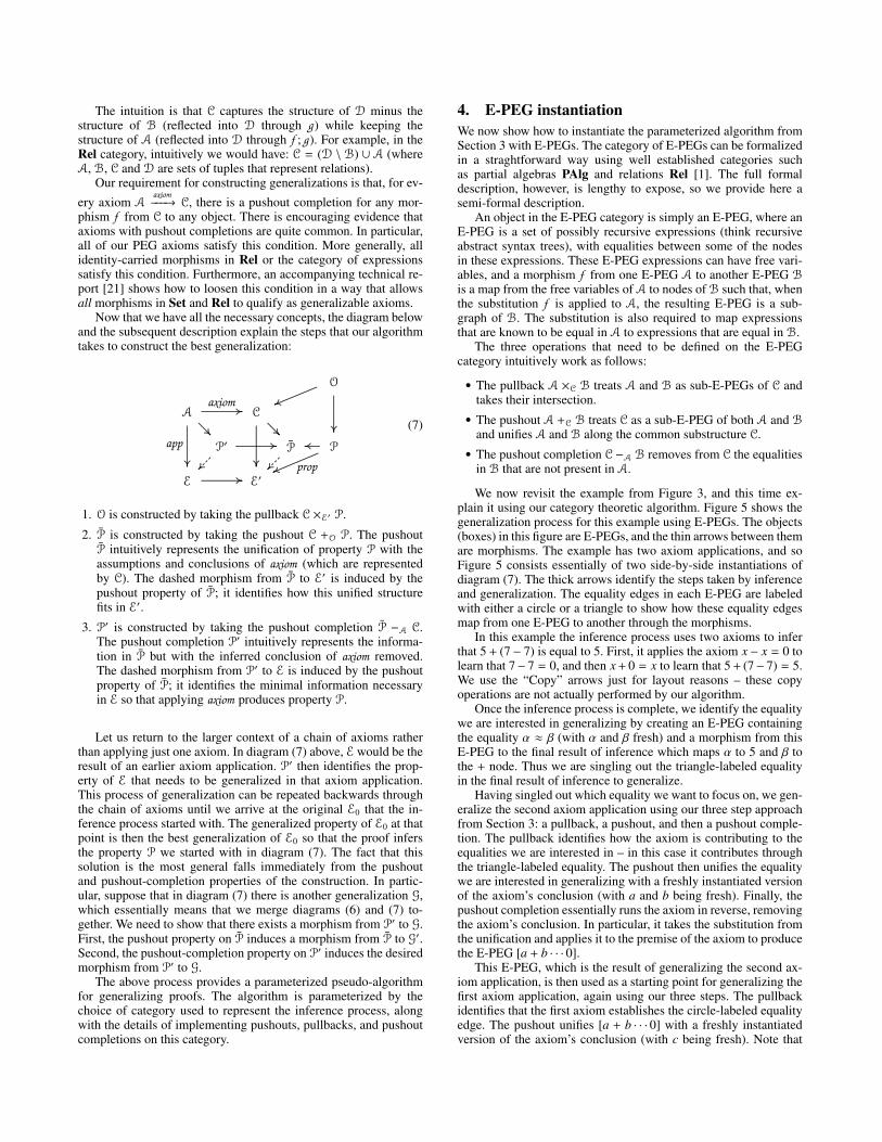
The intuition is that C captures the structure of D minus thestructure of B (reflected into D through g ) while keeping thestructure of A (reflected into D through f ; g ). For example, in theRel category, intuitively we would have: C = (D \ B) ∪ A (whereA, B, C and D are sets of tuples that represent relations).

Our requirement for constructing generalizations is that, for ev-

ery axiom Aaxiom−−−→ C, there is a pushout completion for any mor-

phism f from C to any object. There is encouraging evidence thataxioms with pushout completions are quite common. In particular,all of our PEG axioms satisfy this condition. More generally, allidentity-carried morphisms in Rel or the category of expressionssatisfy this condition. Furthermore, an accompanying technical re-port [21] shows how to loosen this condition in a way that allowsall morphisms in Set and Rel to qualify as generalizable axioms.

Now that we have all the necessary concepts, the diagram belowand the subsequent description explain the steps that our algorithmtakes to construct the best generalization:

A C

E E′

P

O

P′ P

................................................................................... ............axiom

...............................................................................................

app

...............................................................................................

................................................................................... ............

.................................................................................................

............ prop

...........................................................................................

............

.......................................................................................

......................................... ............

........................................

................................................................................... ............

......................................... ............

........................................

..................................................

(7)

1. O is constructed by taking the pullback C ×E′ P.

2. P is constructed by taking the pushout C +O P. The pushoutP intuitively represents the unification of property P with theassumptions and conclusions of axiom (which are representedby C). The dashed morphism from P to E′ is induced by thepushout property of P; it identifies how this unified structurefits in E′.

3. P′ is constructed by taking the pushout completion P −A C.The pushout completion P′ intuitively represents the informa-tion in P but with the inferred conclusion of axiom removed.The dashed morphism from P′ to E is induced by the pushoutproperty of P; it identifies the minimal information necessaryin E so that applying axiom produces property P.

Let us return to the larger context of a chain of axioms ratherthan applying just one axiom. In diagram (7) above, E would be theresult of an earlier axiom application. P′ then identifies the prop-erty of E that needs to be generalized in that axiom application.This process of generalization can be repeated backwards throughthe chain of axioms until we arrive at the original E0 that the in-ference process started with. The generalized property of E0 at thatpoint is then the best generalization of E0 so that the proof infersthe property P we started with in diagram (7). The fact that thissolution is the most general falls immediately from the pushoutand pushout-completion properties of the construction. In partic-ular, suppose that in diagram (7) there is another generalization G,which essentially means that we merge diagrams (6) and (7) to-gether. We need to show that there exists a morphism from P′ to G.First, the pushout property on P induces a morphism from P to G′.Second, the pushout-completion property on P′ induces the desiredmorphism from P′ to G.

The above process provides a parameterized pseudo-algorithmfor generalizing proofs. The algorithm is parameterized by thechoice of category used to represent the inference process, alongwith the details of implementing pushouts, pullbacks, and pushoutcompletions on this category.

4. E-PEG instantiationWe now show how to instantiate the parameterized algorithm fromSection 3 with E-PEGs. The category of E-PEGs can be formalizedin a straghtforward way using well established categories suchas partial algebras PAlg and relations Rel [1]. The full formaldescription, however, is lengthy to expose, so we provide here asemi-formal description.

An object in the E-PEG category is simply an E-PEG, where anE-PEG is a set of possibly recursive expressions (think recursiveabstract syntax trees), with equalities between some of the nodesin these expressions. These E-PEG expressions can have free vari-ables, and a morphism f from one E-PEG A to another E-PEG Bis a map from the free variables of A to nodes of B such that, whenthe substitution f is applied to A, the resulting E-PEG is a sub-graph of B. The substitution is also required to map expressionsthat are known to be equal in A to expressions that are equal in B.

The three operations that need to be defined on the E-PEGcategory intuitively work as follows:

• The pullback A ×C B treats A and B as sub-E-PEGs of C andtakes their intersection.• The pushout A +C B treats C as a sub-E-PEG of both A and B

and unifies A and B along the common substructure C.• The pushout completion C −A B removes from C the equalities

in B that are not present in A.

We now revisit the example from Figure 3, and this time ex-plain it using our category theoretic algorithm. Figure 5 shows thegeneralization process for this example using E-PEGs. The objects(boxes) in this figure are E-PEGs, and the thin arrows between themare morphisms. The example has two axiom applications, and soFigure 5 consists essentially of two side-by-side instantiations ofdiagram (7). The thick arrows identify the steps taken by inferenceand generalization. The equality edges in each E-PEG are labeledwith either a circle or a triangle to show how these equality edgesmap from one E-PEG to another through the morphisms.

In this example the inference process uses two axioms to inferthat 5 + (7 − 7) is equal to 5. First, it applies the axiom x − x = 0 tolearn that 7− 7 = 0, and then x + 0 = x to learn that 5 + (7− 7) = 5.We use the “Copy” arrows just for layout reasons – these copyoperations are not actually performed by our algorithm.

Once the inference process is complete, we identify the equalitywe are interested in generalizing by creating an E-PEG containingthe equality α ≈ β (with α and β fresh) and a morphism from thisE-PEG to the final result of inference which maps α to 5 and β tothe + node. Thus we are singling out the triangle-labeled equalityin the final result of inference to generalize.

Having singled out which equality we want to focus on, we gen-eralize the second axiom application using our three step approachfrom Section 3: a pullback, a pushout, and then a pushout comple-tion. The pullback identifies how the axiom is contributing to theequalities we are interested in – in this case it contributes throughthe triangle-labeled equality. The pushout then unifies the equalitywe are interested in generalizing with a freshly instantiated versionof the axiom’s conclusion (with a and b being fresh). Finally, thepushout completion essentially runs the axiom in reverse, removingthe axiom’s conclusion. In particular, it takes the substitution fromthe unification and applies it to the premise of the axiom to producethe E-PEG [a + b · · · 0].

This E-PEG, which is the result of generalizing the second ax-iom application, is then used as a starting point for generalizing thefirst axiom application, again using our three steps. The pullbackidentifies that the first axiom establishes the circle-labeled equalityedge. The pushout unifies [a + b · · · 0] with a freshly instantiatedversion of the axiom’s conclusion (with c being fresh). Note that

x x x x0

+

7 75

+

7 75 0

+

c ca

+

c ca 0

0

+

ba 0

+

ba 0

+

7 75 0

+

7 75 0

+

yx 0

+

yx 0

+

ba 0

First Axiom Second Axiom

AxiomApplication

Copy

PushoutPushout

Copy

PushoutCompletion

AxiomApplication

PushoutCompletion

PullbackPullback

Identify Equalityto Generalize

Figure 5. Example of generalization using E-PEGs

the circle-labeled equality edge in [a + b · · · 0] must unify with thecorresponding equality edge in the axiom’s conclusion, and so bgets unified with the minus node. Finally, the pushout completionruns the first axiom in reverse, essentially removing the axiom’sconclusion. The result is our generalized starting E-PEG for thatproof. We then generate a rule stating that whenever this startingE-PEG is found, the final conclusion of the proof is added, in thiscase the triangle-labeled equality.

The details of how our E-PEG category is designed affects theoptimizations that our approach can learn. For example, the cate-gory described above has free variables, but they only range overE-PEG nodes. For additional flexiblity, we can also introduce freevariables that range over node operators, such as variables OP1 andOP2 in Figure 1. This would allow us to generate optimizations thatare valid for any operator, for example pulling an operation out of aloop if its arguments are invariant in the loop. For even more flex-ibility, we can augment our E-PEG catgory with domain-specificrelationships on operator variables, which could be used to indi-cate that one operator distributes over another. With this additionalflexiblity, we can learn the more general version of LIVSR show inFigure 1. In all these cases, to learn the more general optimizations,one has to not only add flexiblity to the category, but also re-expressthe axioms so that they take advantage of the more general cate-gory (as was shown in Section 2.1). The E-PEG category can alsobe augmented with new structure in order to accommodate anal-yses not based on equalities. For example, an alias analysis couldadd a distinctness relation to identify when two references point todifferent locations. This would allow our generalization techniqueto apply beyond the kinds of equality-based optimizations that ourPeggy compiler currently performs [22].

5. Other applications of generalizationThe main advantage of having an abstract framework for proof gen-eralization is that it separates the domain-independent componentsof proof generalization — how to combine pullbacks, pushouts, andpushout completions — from the domain-specific components ofthe algorithm — how to compute pullbacks, pushouts, and pushoutcompletions. As a result, not only does this abstraction provides uswith a significant degree of flexibility within our own domain ofE-PEGs, as described in Section 4, but it also enables applicationsof proof generalization to problems unrelated to E-PEGs. We illus-trate this point by showing how our generalization framework from

Section 3 can be used to learn efficient query optimizations in re-lational databases (Section 5.1) and also assist programmers withdebugging static type errors (Section 5.2). Additional applicationsof our proof generalization framework such as type generalization,can be found in the technical report [21].

5.1 Database query optimizationIn relational databases, a small optimization in a query can producemassive savings. However, these optimizations become more ex-pensive to find as the query size grows and as the database schemagrows. We focus here on the setting of conjunctive queries, whichare existentially quantified conjunctions of the predicates definedin the database schema. For example, the query ∃y. R(x, y)∧R(y, z)returns all elements x and z for which there exists a y such that(x, y) and (y, z) are in the R table (relation). For sake of brevity, wediscuss only conjunctive queries without existential quantification.

A conjuctive query can itself be represented as a small database.For example, the query q := R(x, y, z, 1) ∧ R(x′, y, 0, 1) can berepresented by the following database (our notation assumes thereis one table in the database called R and just lists the tuples in R):

Q := x y z 1x′ y 0 1

Any result produced by q on a database instance I corresponds witha relation-preserving and constant-preserving function from Q to I.One nice property of this representation is that the number of joinsrequired to execute a query is exactly one less than the number ofrows in the small database representing the query. Thus, reducingthe number of rows means reducing the number of joins.

Most databases have some additional structure known by thedesigner. One such structure could be that the first column of Rdetermines the third column (we will use A, B, C, and D to referto the columns of R). This is known as a functional dependency,noted by A→ C. Functional dependencies fit into the broader classof equality-generating dependencies since they can be used to in-fer equalities. A query optimizer can exploit this information toreduce the number of variables in a query, identify better opportu-nities for joins, or even identify redundant joins. Unfortunately, thefunctional dependency A → C provides no additional informationfor our example query, at least not yet.

Another form of dependencies is known as tuple-generatingdependencies. These dependencies take the form “if these tuples

are present, then so are these”. One common example is knownas multi-valued dependencies. Suppose in our example database,the designer knows that, for a fixed element in B, column A iscompletely independent of C and D. In other words, R(a, b, c, d) ∧R(a′, b, c′, d′) implies R(a, b, c′, d′), as well as R(a′, b, c, d). This isdenoted as B� A or equivalently as B� CD.

Adding tuples to a query in general is harmful because eachadded tuple represents an additional join. However, combined withequality-generating dependencies, these additional tuples can beused to infer useful equalities, which can then simplify the query.Let us apply an algorithm known as “the chase” [6] to optimize ourexample query using A→ C and B� A:

x y z 1x′ y 0 1

|B�A===⇒

x y z 1x′ y 0 1x y 0 1

|A→C===⇒

x y 0 1x′ y 0 1

The added tuple was used to infer that z must equal 0, whichthen simplifies the rightmost database above into two tuples. Theoptimizer can use this to select only tuples with C equal to 0 beforejoining, a potentially huge savings. Although this example wasbeneficial, many times adding tuples is harmful because it addsadditional joins which can be inefficient. Thus, a query optimizerprefers to infer equalities without introducing unnecessary tuples.

Our framework from Section 3, instantiated to the databasesetting, can use instances of optimized queries to identify generalrules for when adding tuples to a query is helpful. In particular, inthe above example, it could identify exactly what properties of theoriginal query led to the inferred equality. The category we willuse in this example is like Rel but with quaternary relations. The“axiom” A→ C can be expressed categorically by the morphism

a b c da b′ c′ d′

c, c′ 7→ c−−−−−−→

a b c da b′ c d′

The “axiom” B� A can be expressed using the morphism

a b c da′ b c′ d′

→

a b c da′ b c′ d′

a b c′ d′

Applying our framework to our sample query optimization se-quence will produce the theorem

a b c da′ b c′ d′

c, c′ 7→ c−−−−−−→

a b c da′ b c d′

or simply B → C. Thus, our framework can be used to learnequality-generating dependencies, removing the need for the in-termediate generated tuples. This was possible because the de-pendencies involved, namely A → C and B � A, could be ex-pressed categorically as morphisms. We have proven that our learn-ing technique can be used so long as all the dependencies can beexpressed in this manner. Although the primary purpose of apply-ing our framework to database optimizations was to demonstratethe flexibility of our framework, discussions with an expert in thedatabase community [5] have revealed that our technique is in facta promising approach that would merit further investigation.

5.2 Type debuggingAs type systems grow more complex, it also becomes more difficultto understand why a program does not type check. Type systems re-lying on Hindly-Milner type inference [18] are well known for pro-ducing obscure error messages since a type error can be caused byan expression far removed from where the error was finally noticedby the compiler. Below we show how to apply our framework asa type-debugging assistant that is similar to [12], but is also easilyadaptable to additional language features such as type classes.

In Haskell, heap state is an explicit component of a type. Forexample, readSTRef is the function used to read references. Thisis a stateful operation, so it has type ∀s a. STRef s a → ST s a.STRef s a is the type for a reference to a in heap s. ST s a standsfor a stateful computation using heap s to produce a value of type a.In order to use this stateful value, Haskell uses the type class Monadto represent sequential operations such as stateful operations. ThusST s is an instance of Monad for any heap s. A problem that quicklyarises is that operations such as + take two Ints, not two ST s Ints.Thus, + has to be lifted to handle effects. To do this, there isa function liftM2 which lifts binary functions to handle effectsencoded using any Monad. Likewise, liftM lifts unary functions.

Now consider the task of computing the maximum value from alist of references to integers. If the list is empty, the returned valueshould be −∞. In Haskell, integers with −∞ are encoded usingthe Maybe Int type: the Nothing case represents −∞ and theJust n case represents the integer n. Conveniently, max defined onInt automatically extends to Maybe Int. The following programwould seem to accomplish our goal:

maxInRefList refs= case refs of

[] -> Nothingref : tail -> liftM2 max

(liftM Just (readSTRef ref))(maxInRefList tail)

Since readSTRef is a stateful operation, the lifting functionsliftM2 and liftM allow max and Just to handle this state. Unfor-tunately, this program does not type check. The Glasgow HaskellCompiler, when run on the above program using do notation forthe recursive call, produces the error “readSTRef ref has inferredtype ST s a but is expected to have type Maybe a”. This error mes-sage does not point directly to the problem, so the programmer hasto examine the program, possibly even callers of maxInRefList,to understand why the compiler expects readSTRef ref to have adifferent type. Within maxInRefList alone there are many possi-blities, such as the lifting operations, dealing with Maybe correctly,and the recursive call. Here we can apply proof generalization tolimit the scope of where the programmer has to search, therebyhelping identify the cause of the type error.

Type inference can be encoded categorically using a categoryof typed expressions. An object is a set of program expressionsand a map from these program expressions to type expressions,although this map is not required to be a valid typing. Programexpressions can have program variables, and type expressions canhave type variables. A morphism from A to B is a type-preservingsubstitution of program and type variables in A to program and typeexpressions in B such that when the substitution is applied to A, theresulting expressions are sub-expressions of the ones in B. In thiscategory, typing rules can be encoded as morphisms. For example,function application can be encoded as:

(( f : α) (x : β)) : γ (( f : β→ γ) (x : β)) : γ........................................................................................................................ ............α 7→ (β→ γ)

This states that, for any program expressions f and x where x hastype β, f must have type β → γ for f x to have type γ. Hence,the type α of f is mapped to β → γ by the morphism. In effect,applying this axiom unifies the type of f with β→ γ.

Rules for polymorphic values can also be encoded as mor-phisms. For example, the rule for Nothing can be encoded as:

Nothing : α Nothing : Maybe β..................................................................................................................................................................... ............α 7→ Maybe β

This states that, for the value Nothing to have type α, there mustexist a type β such that α equals Maybe β. As before, applying thisaxiom unifies the type of Nothing with Maybe β.

Putting aside type classes for simplicity, the rule for liftM is:

liftM : α liftM : (β→ γ)→ M β→ M γ........................................................................................................................ ............α 7→ . . .

This rule uses a type variable M, which is treated like other typevariables except it maps to unary type constructors, such as Maybeor the partially applied type constructor ST s.

Going back to the maxInRefList example, since the compilerexpects readSTRef ref to have type Maybe a, the type inferenceprocess could be made to produce a proof that this fact must betrue for the program to type check. This proof can be expressedcategorically using the above encoding, which allows us to nowapply our generalization technique. We ask the question “Why doesreadSTRef ref need to have type Maybe a?” categorically usinga morphism from object (x : Maybe ζ) that maps x to readSTRefref and ζ to a. We then proceed backwards through the inferenceprocess. For each step, we determine whether it contributes to theproperty; if it does, we generalize it, otherwise we skip the stepentirely so as not to needlessly constrain the program.

The first useful step to generalize is the function application rulewhere the function is liftM Just and the argument is readSTRefref. During inference, before applying this axiom, liftM Justhad type M a→ M (Maybe α) for some M, a, and α; liftM Just(readSTRef ref) had type Maybe β for some β; and readSTRefref still had the unconstrained type γ. Applying the function ap-plication rule during inference causes γ to be unified with M a andM (Maybe α) with Maybe β. In turn, this forces M to unify withMaybe, contributing to the reason why readSTRef ref must havetype Maybe a. Generalization can analyze this axiom applicationto determine that readSTRef ref has type Maybe a because oftwo key properties: (1) liftM Just had type M a → M δ (whereδ generalizes Maybe α) and (2) liftM Just (readSTRef ref)had type Maybe β (the same as the non-generalized type).

Generalizing property (1) eventually recognizes liftM as animportant value in the program, whereas Just is not. Generalizingproperty (2) reaches similar kinds of conclusions in the rest of theprogram. In this manner, generalization identifies exactly whichcomponents of the program are causing the compiler to expectreadSTRef ref to have type Maybe a. The resulting skeletonprogram is shown below, using dots for irrelevant expressions:

. = case . of. -> Nothing. -> liftM2 . (liftM . .) .

The skeleton program makes it clear that only the two cases, thelifting operations, and the use of Nothing are causing the incor-rect expectation. Combining these three facts, the programmer canquickly realize that they forgot to lift the stateless value Nothinginto the stateful effect ST s, easily fixed by passing Nothing to thereturn function. This mistake was hidden before because Maybe iscoincidentally an instance of Monad, so the lifting functions wereinterpreted as lifting Maybe rather than ST s. The mistake was ina different case than where the error was reported, misleading theprogrammer into examining the wrong part of the program. Gener-alization, however, helps the programmer pinpoint the problem byremoving parts of the program that do not contribute to the error.

6. Manipulating proofsGiven a proof of correctness, our generalization technique producesthe most general optimization for which the same proof applies.This still allows different proofs of the same fact to produce in-comparable generalizations. However, by changing proofs intelli-gently, we can ensure better generalizations. Below we illustratethree classes of proof edits that we use to produce more broadlyapplicable optimizations: sequencing axiom applications, remov-ing irrelevant axiom applications, and decomposing proofs.

6.1 Sequencing axiom applicationsOur generalization technique requires proofs to be represented asa sequence of linear steps. However, proofs are often expressedas trees, in which case one needs to linearize the tree before ourtechnique is applicable. The most faithful encoding of a proof treeis to use “parallel” axiom applications (which are formalized inthe technical report [21]) to directly encode the tree: each stepin the linearized proof corresponds to the parallel application ofall axioms in one layer of the proof tree. This encoding is themost faithful linearization of a proof tree because the tree can bereconstructed from the linearization.

A simpler linearization is to flatten the tree so that each axiomapplication in the linearized proof corresponds to an axiom applica-tion in the proof tree. In this setting, axiom applications that are un-ordered in the tree must somehow be ordered. Unfortunately, whentwo axiom applications have overlapping conclusions, different or-ders in the linearized proof can lead to different and incomparablegeneralizations. Nonetheless, we have shown that no matter whatorder is selected, the generalized result will be equal to or possiblybetter than the result of using the “parallel” encoding which keepsthe tree structure intact. As a result, since sequencing can only help,our implementation sequences axiom applications before general-izing, rather than retaining the parallel encoding.

6.2 Removing irrelevant axiom applicationsSometimes certain axiom applications infer information that is ir-relevant to the final property that we are interested in concluding.An irrelevant axiom application can overly restrict the generalizedoptimization by making certain equalities (those required by theaxiom) seem important to the optimization when they are not. Priorto generalization, it is difficult to identify which steps of the proofare relevant to the optimization. However, since generalization pro-ceeds backwards through the proof, each step of the algorithm caneasily identify when an axiom application is not contributing to thecurrent property being generalized and simply skip it. In essence,our algorithm edits the original proof on the fly, as generalizationproceeds, to remove steps not useful for the end goal.

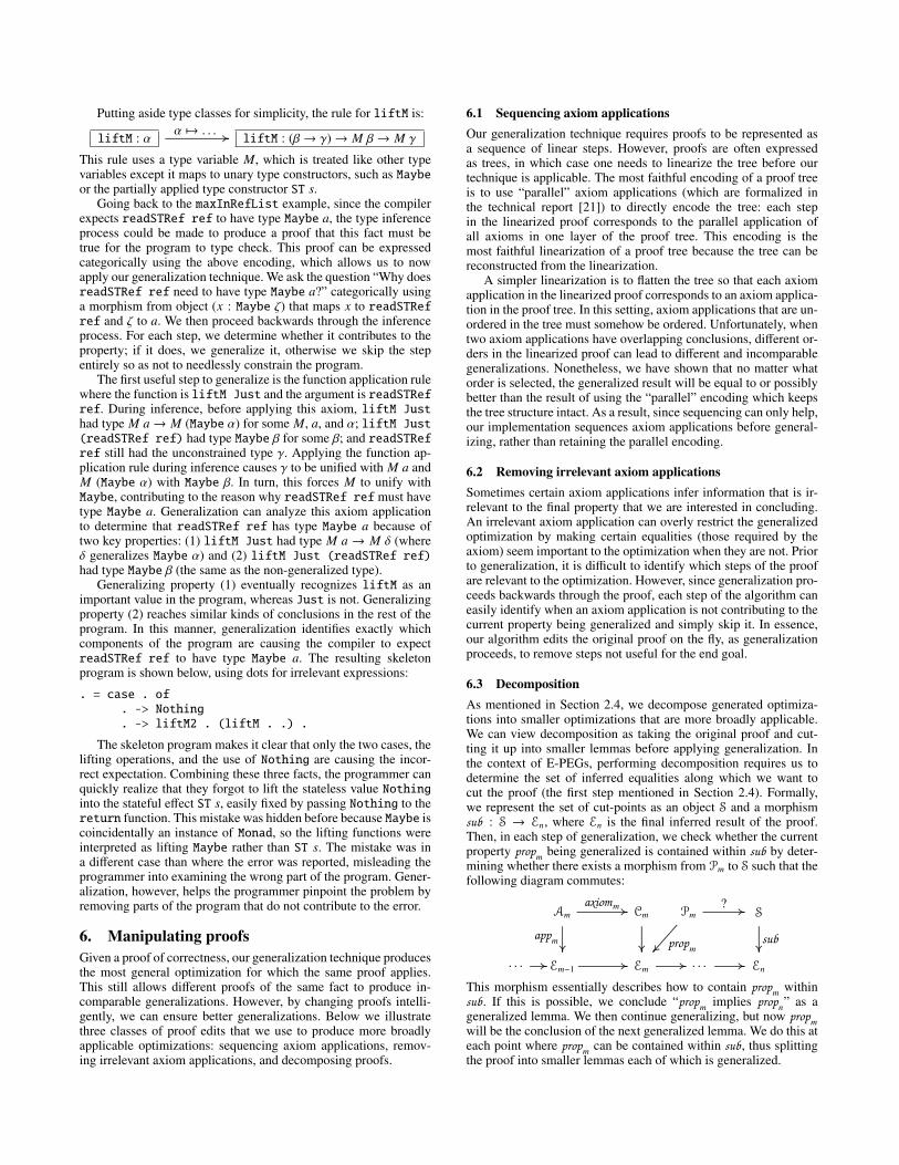
6.3 DecompositionAs mentioned in Section 2.4, we decompose generated optimiza-tions into smaller optimizations that are more broadly applicable.We can view decomposition as taking the original proof and cut-ting it up into smaller lemmas before applying generalization. Inthe context of E-PEGs, performing decomposition requires us todetermine the set of inferred equalities along which we want tocut the proof (the first step mentioned in Section 2.4). Formally,we represent the set of cut-points as an object S and a morphismsub : S → En, where En is the final inferred result of the proof.Then, in each step of generalization, we check whether the currentproperty propm being generalized is contained within sub by deter-mining whether there exists a morphism from Pm to S such that thefollowing diagram commutes:

. . .

Am

Em−1

Cm

Em

Pm

. . . En

S

........................................ ............

.................................................................................................. ............axiomm

...................................................................

appm

...................................................................

............................................................................................... ............

.....................................................................................

propm

............................................................... ............ ............................................................... ............

...................................................................sub

................................................................................... ............?

This morphism essentially describes how to contain propm withinsub. If this is possible, we conclude “propm implies propn” as ageneralized lemma. We then continue generalizing, but now propmwill be the conclusion of the next generalized lemma. We do this ateach point where propm can be contained within sub, thus splittingthe proof into smaller lemmas each of which is generalized.

Optimization DescriptionLIVSR Loop-induction variable SRInter-loop-SR SR across two loopsLIVSR-bounds Optimizes loop bounds after LIVSRILSR-bounds Optimizes loop bounds after Inter-loop-SRFun-specific-opts Function-specific optimizationsSpec-inlining Inline only for special parameter valuesPartial-inlining Inline only part of the calleeTmp-obj-removal Remove temporary objectsLoop-op-Factor Factor op out of loopLoop-op-Distr Distribute op into loop to cancel other opsEntire-loop-SR Replace entire loop with one opArray-copy-prop Copy prop through array elementsDesign-pats-opts Remove overhead of design patterns

Figure 6. Learned optimizations (SR = Strength Reduction)

for (i=0; i<h; i++)for (j=0; j<w; j++)img[i*w+j] /= 2;

�=⇒for (i=0; i<h*w; i+=w)for (j=i; j<i+w; j++)img[j] /= 2;

(a) Concrete example

for (I=E1; I<E2; I++)for (J=0; J<E3; J++)E4(I*E3+J)

�=⇒for (I=E1; I<E2*E3; I+=E3)for (J=I; J<I+E3; J++)E4(J)

where E1, E2, E3, and E4 are any loop-invariant expressions(b) Generated optimization rule

Figure 7. Generalized inter-loop strength reduction

7. Experimental evaluationWe used the Peggy infrastructure [22] and E-PEGs to implementour technique for generating optimizations (as was illustrated inSections 2 and 4). In this section, we experimentally validate threehypotheses about our technique: (1) our technique allows a pro-grammer to easily extend the compiler by sketching what an op-timization looks like with before-and-after examples (2) our tech-nique can amortize the cost of expensive-to-run super-optimizersby generating fast-to-run optimizations and (3) our technique caneven learn optimizations that are significantly profitable on codethat the compiler was not trained on.

7.1 Extending the compiler through examplesWhen the compiler does not perform an optimization that the pro-grammer would like to see, our technique allows the programmerto train the compiler by providing a concrete example of what thedesired optimization does. By using our implementation to learna variety of optimizations in this way, we demonstrate experimen-tally that our technique enables the compiler to be extensible in aneasy-to-program way, without the programmer having to learn anynew language or compiler interface.

The optimizations that our system learned from examples arelisted in Figure 6. It took on average 3.5 seconds to learn each ex-ample (including translation validation). The only optimizations inthis list that are performed by gcc -O3 are LIVSR and Array-copy-prop. This demonstrates the benefit of our system: it allows an end-user programmer to easily implement non-standard optimizationstargeting application domains with high-performance needs, suchas computer graphics, image processing, and scientific computing.

The LIVSR optimization was already shown in Section 2. Op-timizations LIVSR-bounds through Loop-op-Factor will be cov-ered throughout the remainder of Section 7. We start with Inter-loop-SR and ILSR-bounds. These optimizations apply to a com-mon programming idiom in image processing, which is shown in

len = array.length;sum = 0;for (i=0; i<len; i++)sum += array[i] * 7;

�=⇒

len = array.length;sum = 0;for (i=0; i<len; i++)sum += array[i];

sum *= 7;

(a) Concrete example

X = 0while (E1)X += E2 * E3

�=⇒

X = 0while (E1)X += E2

X *= E3

where E3 is a loop-invariant expression(b) Generated optimization rule

Figure 8. Loop-operation factoring

the left part of Figure 7(a). The img variable is a two-dimensionalimage represented as a one-dimensional array in row-major form.Programmers commonly use this kind of representation to effi-ciently store dynamically-sized two-dimensional images. The orig-inal code in Figure 7(a) uses a convenient way of iterating oversuch arrays, whereas the transformed code uses the more efficient,yet harder to program, formulation that programmers typically use(it removes the multiplication and addition from the inner loop).From the concrete instance, our generalizer determines that the imgarray is actually insignificant (the only part that matters is the i*w+ j computation); it determines that the starting point of the outerloop is insignificant; and that the bounds on both loops can be gen-eralized into loop invariant expressions. Furthermore, although weshow the learned optimization as one rule, our decomposition algo-rithm would split this into two optimizations: one which optimizesthe body of the loop (Inter-loop-SR), and one which optimizes thebounds of the loop (ILSR-bounds). A similar decomposition whenlearning LIVSR would also produce LIVSR-bounds. Also, all ourgenerated optimization rules — including the one in Figure 7(b) —can apply to programs containing other statements in the loops thatdo not affect the significant program fragments being optimized.

When traditional compilers like gcc -O3 do not perform theoptimization described above, an image-processing programmerwould be forced to use the more efficient but error-prone version ofthe code. With our system, the programmer can use the simpler ver-sion and rely on the compiler to optimize it into the more efficientone. Furthermore, if the programmer encounters a new instance ofthe programming pattern that the generated rule does not cover, theprogrammer can train the compiler with another example. This sce-nario emphasizes how easy it is for non-compiler-experts to benefitfrom our system. Extending the compiler is as simple as provid-ing a single concrete example, without having to worry about theside conditions required for correctness or having to learn a newlanguage — like the language in Figure 7(b), including expressionvariables like E1 and side conditions like “E1 is loop-invariant”.

We next show another example of an optimization not per-formed by gcc -O3, loop-operation factoring (Loop-op-Factor inFigure 6). The concrete example that we used to sketch the op-timization is shown in Figure 8(a). The multiplication inside theloop gets factored out of the loop through the additions. The gen-eralization that our system generates is shown in Figure 8(b). Ourgeneralizer determined that the use of the array is insignificant andthe format of the loop is insignificant, as is the constant 7, whichcan in fact be any loop-invariant expression.

Finally, we show how our system can learn several optimiza-tions for the power function from Figure 9. Starting with the con-crete optimization instance pow(a, p) * pow(b, p) �⇒ pow(a* b, p), our generalizer shows that the two concrete programsare equivalent, and then generalizes the example into the optimiza-

int pow(int base, int power)int prod = 1;for (int i = 0; i < power; i++)prod *= base;

return prod;

Figure 9. The power function for integers

tion ∀x, y, z ∈ int. pow(x, z) * pow(y, z) �⇒ pow(x * y, z). Thisis an example of Fun-specific-opts from Figure 6. Similarly, wewere able to get our generalizer to learn the non-trivial optimiza-tion: ∀x ∈ uint. pow(2, x) �⇒ 1 � x (which is an example ofSpec-inlining in Figure 6). Here again, neither of these optimiza-tions are performed by gcc -O3, whereas our approach allows theprogrammer to easily specify these optimizations by example.

7.2 Learning from super-optimizersAnother possible use of our approach is to amortize the cost of run-ning a super-optimizer. Given an input program, a super-optimizerperforms a brute force exploration through the large space of trans-formed programs to find the (near) optimal version of the inputprogram. Our approach can mitigate the cost of running super-optimizers by learning optimizations from one run of the super-optimizer, and then applying only the learned optimizations to getmuch of the benefit of the super-optimizer at a fraction of the cost.

The Peggy compiler at its core performs a super-optimizer-stylebrute-force exploration by applying axioms to build an E-PEG thatcompactly represents exponentially many different versions of theinput program, and then using a profitability heuristic to find thebest PEG represented in this E-PEG. To evaluate our approach inthe setting of super-optimizers, we used Peggy to super-optimizesome microbenchmarks and SpecJVM, and used our technique onthe original and transform programs to learn optimizations.

Several of the optimizations learned using before-and-afterexamples in Section 7.1 cannot be learned by using the super-optimizer – they really do require a programmer to give aninput-output example. For instance, if the Peggy super-optimizerwere given pow(a,p)*pow(b,p) to optimize using basic axioms,it would not be able to find the desired transformed programpow(a*b,p) because, even though it can decompose the originalexpression into smaller pieces, it cannot guess how to reassemblethem into pow(a*b,p). However, Peggy can prove the original andtransformed programs equivalent because it sees the pow(a*b,p)term to which it can apply axioms. In essence it is easier to applyaxioms on the original and transformed programs, and meet in themiddle, rather than derive the transformed program from the origi-nal. With the proof, our approach can learn a new optimization thatthe Peggy super-optimizer would not have performed.

Our super-optimizer experiments also show how inlining com-bined with generalization produces useful and unconventional opti-mizations. Inlining in Peggy simply adds the information that a callnode is equivalent to the body of the called function. Adding thisequality does not force Peggy to choose the inlined version; it justprovides more options in the caller’s E-PEG for the profitabilityheuristic to choose from. When running on code that uses the powfunction from Figure 9, the super-optimizer applied the inlining ax-iom on pow, thus pulling the body of pow into the E-PEG. Peggythen exploited the fact that pow does not affect the heap to optimizethe surrounding context, but chose not to inline pow in the final re-sult. From this our generalizer learned the optimization that pow isheap-invariant; in future compilations, Peggy can immediately usethe fact that pow does not affect the heap to optimize the surround-ing context without the expensive process of inlining pow. This isan example of what we call partial inlining (Partial-inlining in Fig-ure 6), where the optimizer exploits the information learned from

inlining without opting to inline the function. Another example ofpartial inlining we observed involved a large function that modi-fies the heap but always returns 0. By applying the inlining axiom,Peggy was able to optimize the surrounding context with the infor-mation that the return value was 0, but then chose not to inline thecalled function because it was too large. In this case the generalizerwould learn that the function always returns 0, which can be usedin future compilations without having to apply the inlining axiom.

We evaluate the effectiveness of amortizing the cost of a super-optimizer on the SpecJVM suite. For each class in SpecJVM, asa first step we used the Peggy super-optimizer to compile theclass using basic axioms, and used our generalization techniqueto generate a set of optimizations for that class. As a second step,we removed all the basic axioms from Peggy and re-optimized theclass using the axioms that were learned in the first step. Acrossall benchmarks, it took on average 11.15 seconds to generalize amethod, and the average cost of compiling each method went downfrom 26.64 seconds in the first step to 1.47 seconds in the secondstep, while still producing the same output programs.

These experiments show that, for expensive super-optimizers,our technique can improve compilation time while still produc-ing the same result. Furthermore, our benchmark-specific optimiza-tions can still apply even if small changes are made to the code.As a result, we can avoid a super-optimizing compile after eachsmall change, while still retaining many of the benefits of the super-optimizer. Eventually, however, the learned optimizations will goout of date, at which point a super-optimizing compile would beneeded. Thus, we envision that our approach could be used to per-form an expensive super-optimization run every so often while us-ing the generated optimizations in between.

7.3 Cross-trainingThe above experiment illustrates the benefits of learning optimiza-tions when compiling exactly the same code that was learned on.We now show some encouraging evidence that even cross-trainingis possible. Our hypothesis is that many libraries are used in styl-ized ways, and so training with Peggy’s super-optimizer on someuses of a library can discover optimizations that would be useful onpreviously unseen code that uses the same library.

We conducted a preliminary evaluation of this hypothesis ona Java ray tracer that uses a functional vector library. Peggy’soptimization phase improves this benchmark’s performance by 7%,compared to only using Sun’s Java 6 JIT, by removing the short-lived temporary objects (Tmp-obj-removal in Figure 6).

Most of these gains come from one important method, call it m.We identified another vector-intense method, call it f, to train ourlearning optimizer on. Using only the axioms learned from opti-mizing the expressions within f, Peggy was able to optimize m toproduce a 3.1% runtime improvement on the ray tracer, instead ofthe 7.1% speed-up gained by fully optimizing m. Alternatively, us-ing a slightly larger training set produces a 5.1% speed-up. Uponfurther investigation, we found that the learned optimizations per-form large-step simplifications of common usage patterns of thevector library (for example, a vector-scale followed by a vector-add). Furthermore, if in addition to the learned optimizations fromeither training set, we allow Peggy to also use those original ax-ioms which infer equalities without creating any new terms (41%of all axioms), Peggy produces the fully optimized m. The purposeof these axioms is to simplify a program, so they cannot lead theoptimizer down a fruitless path. Using simplifying axioms alone onm produces only a 0.6% speed-up. Thus, the optimizations learnedfrom either training set lead the optimizer in the right direction,and the remaining axioms simplify the resulting expressions intothe fully optimized m. These findings show that our technique canbe effective at cross-training even on a small training set.

8. Related workThere has been a long line of work on making optimizers extensibleor easier to develop, including Sharlit [23], Whitfield and Soffa’sGospel system [24], the Broadway extensible compiler [11], andthe Rhodium system for expressing optimizations [14, 15]. In allthese systems, however, the programmer has to learn a new lan-guage or compiler interface to express optimizations. In contrast,our approach learns an optimization from a single example pro-vided by the programmer in a language already familiar to them.

In the context of machine learning, our approach is an instanceof Explanation-Based Learning (EBL) [9]. EBL refers to learningfrom a single example using an explanation of that example. EBLhas been applied to a wide variety of domains, such as Prolog op-timization [10], logic circuit designs [8], and software reuse [3].Many of these applications use algorithms based on unification orProlog [7, 8, 10]. The declarative components of Prolog can be en-coded in our framework by combining categories of expressionswith categories of relations. Furthermore, most EBL implementa-tions provide no guarantees on what is learned, while we can provethat our technique learns the most general lesson for a given expla-nation. Within EBL, our work is closely related that of Dietzen andPfenning [7]. They use λProlog to extend EBL to higher-order andmodal logic, and apply this framework to various settings includingprogram transformations. However, they do not investigate waysto automatically train the optimizer, relying instead on the user toprove the transformation correct using tacticals. As a consequence,they do not attempt to decompose an optimization into subopti-mizations, since a user manually proving an optimization wouldalready do this. Furthermore, we experimentally demonstrate thatgeneralization can be useful for extending compilers and amortiz-ing the cost of super-optimizers.

Aside from EBL, there have been other uses of machine learningin the context of compiler optimizations. Techniques like geneticalgorithms, reinforcement learning, and supervised learning, havebeen used to generate effective heuristics for instruction schedul-ing [17, 20], register allocation [20], prefetching [20], loop-unrollfactors [19], and for optimization ordering [4]. In all these cases,the parts being learned are not the transformation rules themselves,but profitability heuristics, which are functions that decide whenor where to apply certain transformations. As a result, these tech-niques are complementary to our technique: we generate the opti-mization rules themselves, but not the profitability heuristics (weuse a single global profitability heuristic for all optimizations).Also, while modern machine learning techniques use statisticalmethods over large data sets, our EBL-based approach can learnfrom a very small dataset, even from just one example.

The idea of discovering optimizations has also been beenexplored in the setting of super-optimizers [2, 13, 16]. Super-optimizers try to discover optimizations by a brute-force explo-ration of possible transformed programs for a given input program.Traditional super-optimizers find concrete optimization instances,whereas our approach starts with optimization instances, andtries to generalize the instances into reusable optimization rules.As such, our work is complementary to super-optimization tech-niques. However, Bansal and Aiken’s recent super-optimizer [2]does achieve a simple form of generalization, namely abstractionof register names and constants. In contrast, we perform a moresophisticated kind of generalization based on the reasons why theoriginal and transformed programs are equivalent.

Acknowledgments We thank Suresh Jagannathan, Todd Mill-stein, Zachary Tatlock and the anonymous reviewers for their in-valuable feedback on earlier drafts of this paper, as well as AlinDeutsch, Daan Leijen, and Rustan Leino for their feedback on al-ternative applications of proof generalization.

References[1] J. Adamek, H. Herrlich, and G. E. Strecker. Abstract and Concrete

Categories: The Joy of Cats. John Wiley & Sons, 1990.

[2] S. Bansal and A. Aiken. Automatic generation of peepholesuperoptimizers. In ASPLOS, 2006.

[3] R. Bergmann. Explanation-based learning for the automated reuse ofprograms. In CompEuro, 1992.

[4] K. D. Cooper, D. Subramanian, and L. Torczon. Adaptive optimizingcompilers for the 21st century. The Journal of Supercomputing,23(1):7–22, Aug. 2002.

[5] A. Deutsch. Author of [6]. Personal communication, July 2009.

[6] A. Deutsch, A. Nash, and J. Remmel. The chase revisited. In PODS,2008.

[7] S. Dietzen and F. Pfenning. Higher-order and modal logic as aframework for explanation-based generalization. Machine Learning,9(1):23–55, June 1992.

[8] T. Ellman. Generalizing logic circuit designs by analyzing proofs ofcorrectness. In IJCAI, volume 1, pages 643–646, 1985.

[9] T. Ellman. Explanation-based learning: a survey of programs andperspectives. ACM Computing Surveys, 21(2):163–221, June 1989.

[10] M. Gandhe and G. Venkatesh. Improving prolog performance byinductive proof generalizations. In Knowledge Based ComputerSystems, 1990.

[11] S. Z. Guyer and C. Lin. Broadway: A compiler for exploiting thedomain-specific semantics of software libraries. Proceedings ofIEEE, 93(2), 2005.

[12] C. Haack and J. B. Wells. Type error slicing in implicitly typedhigher-order languages. Science of Computer Programming, 50(1-3):189–224, 2004.

[13] R. Joshi, G. Nelson, and K. Randall. Denali: a goal-directedsuperoptimizer. In PLDI, June 2002.

[14] S. Kundu, Z. Tatlock, and S. Lerner. Proving optimizations correctusing parameterized program equivalence. In PLDI, 2009.

[15] S. Lerner, T. Millstein, E. Rice, and C. Chambers. Automatedsoundness proofs for dataflow analyses and transformations via localrules. In POPL, 2005.

[16] H. Massalin. Superoptimizer: a look at the smallest program. InASPLOS, 1987.

[17] A. McGovern, J. E. B. Moss, and A. G. Barto. Building a basicblock instruction scheduler with reinforcement learning and rollouts.Machine Learning, Special Issue on Reinforcement Learning,49(2/3):141–160, May 2002.

[18] R. Millner. A theory of type polymorphism in programming. Journalof Computer and System Sciences, 1978.

[19] M. Stephenson and S. Amarasinghe. Predicting unroll factors usingsupervised classification. In CGO, Mar. 2005.

[20] M. Stephenson, S. Amarasinghe, M. Martin, and U.-M. O’Reilly.Meta optimization: Improving compiler heuristics with machinelearning. In PLDI, June 2003.

[21] R. Tate, M. Stepp, and S. Lerner. Generating compiler optimizationsfrom proofs. Technical report, University of California, San Diego,Nov. 2009.

[22] R. Tate, M. Stepp, Z. Tatlock, and S. Lerner. Equality saturation: anew approach to optimization. In POPL, Jan. 2009.

[23] S. W. K. Tjiang and J. L. Hennessy. Sharlit – A tool for buildingoptimizers. In PLDI, 1992.

[24] D. L. Whitfield and M. L. Soffa. An approach for exploring codeimproving transformations. ACM Transactions on ProgrammingLanguages and Systems, 19(6):1053–1084, Nov. 1997.