generatingsyntheticrdfdatawithconnected blank...

Generating Synthetic RDF Data with Connected

Blank Nodes for Benchmarking

Christina Lantzaki, Thanos Yannakis, Yannis Tzitzikas, and Anastasia Analyti

Computer Science Department, University of Crete,Institute of Computer Science, FORTH-ICS, GREECE{kristi,yannakis,tzitzik,analyti}@ics.forth.gr

Abstract. Generators for synthetic RDF datasets are very importantfor testing and benchmarking various semantic data management tasks(e.g. querying, storage, update, compare, integrate). However, the cur-rent generators do not support sufficiently (or totally ignore) blank nodeconnectivity issues. Blank nodes are used for various purposes (e.g. fordescribing complex attributes), and a significant percentage of resourcesis currently represented with blank nodes. Moreover, several semanticdata management tasks, like isomorphism checking (useful for checkingequivalence), and blank node matching (useful in comparison, version-ing, synchronization, and in semantic similarity functions), not only haveto deal with blank nodes, but their complexity and optimality dependson the connectivity of blank nodes. To enable the comparative evalua-tion of the various techniques for carrying out these tasks, in this paperwe present the design and implementation of a generator, called BGen,which allows building datasets containing blank nodes with the desiredcomplexity, controllable through various features (morphology, size, di-ameter, density and clustering coefficient). Finally, the paper reportsexperimental results concerning the efficiency of the generator, as wellas results from using the generated datasets, that demonstrate the valueof the generator.

1 Introduction

Several works (e.g. [10]) have demonstrated the usefulness of blank nodes forthe representation of the Semantic Web data. In a nutshell, from a theoreticalperspective blank nodes play the role of the existential variables and from atechnical perspective, as gathered in [2], they give the capability to (a) describemulti-component structures, like the RDF containers, (b) apply reification (i.e.provenance information), (c) represent complex attributes without having toname explicitly the auxiliary node (e.g. the address of a person consisting ofthe street, the number, the postal code and the city) and (d) offer protection ofthe inner information (e.g. protecting the sensitive information of the customersfrom the browsers). In [10] the authors survey the treatment of blank nodes inRDF data and prove the relatively high percentages of their usage. Indicatively,and according to their results, the data fetched from the ‘rdfabout.com’ domain

Authors Suppressed Due to Excessive Length

and the ‘opencalais.com’ domain, both of them parts of the LOD (Linked OpenData) cloud, consist of 41.7% and 44.9% of blank nodes, respectively.

However, their existence requires special treatment in various tasks. For in-stance, [10] states that the inability to match blank nodes increases the delta size(the number of triples that need to be deleted and added in order to transformone graph to another) and does not assist in detecting the changes between sub-sequent versions of a Knowledge Base, while [15] proves that building a mappingbetween the blank nodes of two compared Knowledge Bases that minimizes thedelta size is NP-Hard in the general case. In [6] it is proved that (a) decidingsimple or RDF/S entailment of RDF graphs is NP-Complete, and (b) decidingequivalence of simple RDF graphs is Isomorphism-Complete. In [8], a tutorialon how to publish Linked Data, the authors state that it becomes much moredifficult to merge data from different sources when blank nodes are used, as thereis no URI to serve as a common key. However we should note that the abovetasks become tractable for the cases of non-directly connected blank nodes. Still,more complex blank node structures (i.e. cyclic) occur in practice. Indicatively,in [10] 1.6% of the structures are cyclic, while when querying the LOD CloudCache endpoint1 we found out that it contains around 19 millions of blank nodesand almost 30 thousands of them participate in cyclic blank node structures.

In the face of strong identification needs, skolemization2 is suggested, thatreplaces (some or all of) the anonymous resources with globally unique URIs.However, we will never “escape” from blank nodes. Even if we assign to all blanknodes URIs, we are obliged to treat them as unnamed elements when comparingor integrating data. For example, suppose that we want to integrate personaldata from two or more sources where URIs are used for addresses (an addressgroups a street, a number, a city, etc). If we do not treat addresses as blanknodes, then we will treat all addresses as different, and thus we will end up withvery poor information integration. We should also note that blank nodes is not anidiosyncratic feature of RDF. They occur everywhere; consider for instance theworld of relational databases, and suppose that the same information is storedin two different relational databases, each supporting two different policies forautokeys. If we compare these databases then we would like to conclude that theyare identical, but without treating the autokeys as blank nodes this is obviouslyimpossible.

As regards the tasks in which blank nodes require special treatment, studiesare oriented towards either finding special cases where the problems becometractable, or constructing algorithms that approximate the optimal solutions.Indicatively, [15] elaborates on a special case (i.e. RDF graphs with no directlyconnected blank nodes) where the problem of finding the optimal blank nodesmapping is solved in polynomial time, and provides two polynomial algorithmsthat approximate this mapping and can be used in the general case. One of themcan map 150 thousands of bnodes in around 10 seconds. Another notable instanceis [14], where the authors introduce the concept of bounded treewidth to prove

1 http://lod.openlinksw.com/sparql/2 http://www.w3.org/TR/rdf11-concepts/#section-skolemization

Title Suppressed Due to Excessive Length

that entailment checking can be efficient for RDF blank node structures thathave bounded treewidth. Other works avoid matching blank nodes and insteadmake some quite simplistic assumptions (e.g. [9] for studying the dynamics ofLinked Data).

In any of the above cases, an integrated benchmark would be really useful inorder to create a common way to evaluate and compare these (and forthcoming)works. To fill this gap, in this paper we present the design and implementationof a generator, called BGen, which allows building big datasets containing blanknodes satisfying particular connectivity requirements. BGen is not the first RDFgenerator; there are several examples of RDF generators (described in Section 2).However, none of them deals sufficiently with the issue of benchmarking meth-ods that become hard in the presence of blank nodes. The main objective of thisgenerator is to create datasets with blank nodes of variable complexity. Key ele-ment for controlling the complexity of blank nodes is the notion of BComponent

which is essentially a maximal sub-graph of blank nodes that is part of the wholegraph. Having isolated this component we can control its complexity, throughfeatures like the size, the diameter, the density and the clustering coefficient.

The key contribution of this work is that we provide a method to producevariable in size and in complexity blank node components supporting a plethoraof configuration parameters; including diameter, density, clustering coefficient,as well as a parameter for controlling the similarity of the named resources con-nected to the blank nodes. With the introduced method we can produce biggraphs in size under a plausible time and without main memory problems. Wealso provide evidence that the selected features succeed in capturing the com-plexity that is crucial for the intended tasks, by reporting experimental resultsof blank node matching over the produced datasets.

The rest of this paper is organized as follows. Section 2 describes relatedgenerators and introduces the basic requirements of BGen. Section 3 describesthe generator, i.e. its schema, parameters and phases. Section 4 reports exper-imental results regarding time and space, as the generated datasets are scaledup, and uses the generated datasets to evaluate an approximation task. Finally,Section 5 concludes the paper and identifies issues for further research. Moreinformation is available in the Web3.

2 Related Work

Benchmarking in RDF is focused on the performance evaluation of the SemanticWeb repositories. Some notable benchmark tools and works follow. The LehighUniversity Benchmark (LUBM) [5, 4] aims at benchmarking systems with respectto use in OWL applications with large repositories. For data generation, theyhave built the UBA (Univ-Bench Artificial) data generator, that features randomand repeatable data generation. The minimum unit of data generation is theuniversity and for each university a set of OWL files describing its departments(e.g. courses, students, professors) are generated.

3 http://www.ics.forth.gr/isl/bnodeland


The BSBM benchmark [1] is built around an e-commerce use case, and itsdata generator supports the creation of arbitrarily large datasets using the num-ber of products as scale factor.

The Social Intelligence BenchMark (SIB) [11] is an RDF benchmark thatintroduces the S3G2 (Scalable Structure-correlated Social Graph Generator) forgenerating social graphs that contain certain structural correlations. Regardingqualitative evaluation, they evaluate the ability to have some plausible corre-lation in the data, while regarding quantitative evaluation, they evaluate scal-ability in terms of various parameters like clustering coefficient, average pathlength and number of the users. Even though S3G2 offers correlation betweenthe graph structure and the generated data, it does not handle blank nodes andtheir connectivity issues.

A slightly adjusted version of the UBA generator was used to generate syn-thetic data with blank nodes in [15]. However, that version supports a limitedset of control parameters (e.g. it does not support control over cycles, clusteringcoefficient etc); consequently it is not convenient for benchmarking.

To the best of our knowledge there is no generator in the literature thatdeals with the generation of blank nodes adequately. Although there is not anyparticular difficulty in adjusting an already existing generator to produce blanknodes, the difficulty arises when the blank nodes should be connected underparticular connectivity patterns. These patterns differentiate from the previous,as the performance criteria of the evaluated functions are different, too. To fillthis gap in this paper we focus on connectivity issues between the blank nodesof the instance layer.

3 The BGen Generator

At first we describe the requirements of the generator (§3.1), the RDF/S schemathat we have defined (§3.2), and provide a simple instantiation example of thatschema which also introduces the notion of BComponent (§3.3). Then, we analyzehow we control the structural complexity of a BComponent (§3.4), and finallywe present the main algorithm and its phases (§3.5 - §3.7).

3.1 Requirements

Here we list the main requirements, while in Section 3.5 we describe how BGenmeets these requirements.A. Correlation of data. The generator should produce resources that are notrandomly correlated in order to control the structure of the generated dataset and gain realism. A sensible method to implement such a correlation is toproduce data over a specific real-world-like schema that supports various kindsof relationships (i.e. one-to-one, one-to-many, many-to-many).B. Scaling of data. The generator should be able to generate big datasets suitablefor evaluating how the tasks/applications (or the RDF systems upon which theyare built) scale.C. Generation of anonymous data. The generator should support the creation


of blank nodes as a percentage of the totally generated resources.D. Connectivity in anonymous data. The generator should allow controlling theway blank nodes are connected using various features like diameter, density,clustering coefficient. The connectivity between the anonymous and the nameddata should also be controlled (through the schema and a similarity mode).

3.2 The Social Network Schema

Analogously to the UBA generator [5], we have created a schema that describessome basic classes and relations inside a social network. It is illustrated as aUML class diagram in Figure 1. A social network is the minimum unit of datageneration. The primitive building block of this network is the class Person

representing the members of this network. Each person has its personal info, de-scribed through its name (first name and last name), its address (street, zipcode,number and city), its gender and its birth date. Additionally, it has one or morepublic messages (where each public message is characterized by its content andits date). The instance personal info has its own security mode, which can getone of the following values: FriendsOnly, Public, Private.

Fig. 1. The Social Network Schema of BGen

Each person is also connected with other persons through the hasFriend

property indicating who is friend of whom. Apart from the friendship connec-tions, other relationships (parentOf, siblingOf) can be created, too.

The class diagram of Figure 1 is represented in RDF/S and all classes arerepresented as instances of the rdfs:Class, while the ranges of their attributesare represented as subclasses of the rdfs:Literal. The enumeration classes


(Gender mode, Security mode) are represented through the owl:DataOneOf. Tomake the schema as realistic as possible, some restrictions were applied basedon common sense and domain investigation: they are denoted in Figure 1 by themultiplicities of the depicted associations, e.g. each person has one personal info,while it can have more than one public messages and friends.

3.3 Instantiating the Social Network Schema: Example

Here we provide an example showing how the schema is instantiated. Figure 2shows a person (always represented as a blank node instance) accompanied withits personal info, its messages etc. inside a social network, named sn:socialNet1

(always represented as a URI instance). We shall call this a BPerson instantia-

tion.

��

��

��

��

��

��

��

��

��

��

��

��

��

!��"

#�$%��$&'�(��(

��%��

��

��

��

��

��

��

��

��

��%��

)��*

��+��

��,��

��

��

Fig. 2. A simple instantiation paradigm

The decision on how many of the generated instances inside a BPerson in-

stantiation will be presented as blank nodes is based on a parameter named|bPer|, where |bPer| ≥ 1 (i.e. a person is always instantiated as blank node),while |uPer| controls how many will be presented as URIs. For the BPerson

instantiation of Figure 2 we can see that |bPer| = 4 and |uPer| = 3 (3 URIinstances). Although all classes of the social network schema can potentiallyacquire blank nodes as instances, the classes City and Activity are instantiatedonly by URIs because these resources need to be identified and indicated locallyand even globally in real-world-like datasets.

Notice that each BPerson instantiation produces exactly one maximal treeof blank nodes, that is called bTree (nodes and edges in bold in Figure 2). Morecomplex structures of blank nodes (e.g. cycles) require more than one BPerson

instantiations to be connected and will be analyzed later. For the case where|bPer| = 1 the bTree is actually a single node and its height is 0, while as |bPer|increases it becomes wider and its height can come up to 2 (the schema itself


poses this upper bound, as the longest paths that can be created for a BPerson

instantiation is hasPersonalInfo-address and hasPersonalInfo-name).For comprehension reasons we further separate a BPerson instantiation into

two parts: (a) the isolated part that contains the personal information, the ac-tivities, and the public message(s) (upper right part of Figure 2), and (b) theconnection part that contains all the connections of the person with other per-

sons (lower left part). These connections are achieved through the propertieshasFriend and parentOf (or siblingOf).

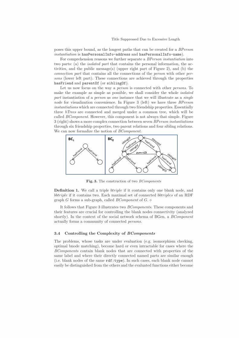
Let us now focus on the way a person is connected with other persons. Tomake the example as simple as possible, we shall consider the whole isolated

part instantiation of a person as one instance that we will illustrate as a single

node for visualization convenience. In Figure 3 (left) we have three BPerson

instantiations which are connected through two friendship properties. Essentiallythree bTrees are connected and merged under a common tree, which will becalled BComponent. However, this component is not always that simple. Figure3 (right) shows a more complex connection between seven BPerson instantiations

through six friendship properties, two parent relations and four sibling relations.We can now formalize the notion of BComponent.

��

��

Fig. 3. The construction of two BComponents

Definition 1. We call a triple btriple if it contains only one blank node, andbbtriple if it contains two. Each maximal set of connected bbtriples of an RDFgraph G forms a sub-graph, called BComponent of G. ⋄

It follows that Figure 3 illustrates two BComponents. These components andtheir features are crucial for controlling the blank nodes connectivity (analyzedshortly). In the context of the social network schema of BGen, a BComponent

actually forms a community of connected persons.

3.4 Controlling the Complexity of BComponents

The problems, whose tasks are under evaluation (e.g. isomorphism checking,optimal bnode matching), become hard or even intractable for cases where theBComponents contain blank nodes that are connected with properties of thesame label and where their directly connected named parts are similar enough(i.e. blank nodes of the same rdf:type). In such cases, each blank node cannoteasily be distinguished from the others and the evaluated functions either become


more time consuming, or their output deviates significantly from the optimal one.Therefore, the following parameters are critical for controlling the BComponents

and generating the desired datasets.

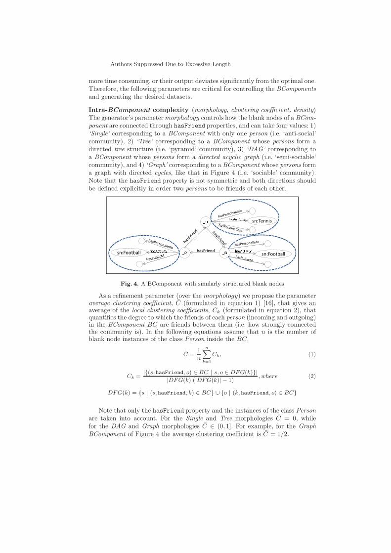
Intra-BComponent complexity (morphology, clustering coefficient, density)The generator’s parametermorphology controls how the blank nodes of a BCom-

ponent are connected through hasFriend properties, and can take four values: 1)‘Single’ corresponding to a BComponent with only one person (i.e. ‘anti-social’community), 2) ‘Tree’ corresponding to a BComponent whose persons form adirected tree structure (i.e. ‘pyramid’ community), 3) ‘DAG’ corresponding toa BComponent whose persons form a directed acyclic graph (i.e. ‘semi-sociable’community), and 4) ‘Graph’ corresponding to a BComponent whose persons forma graph with directed cycles, like that in Figure 4 (i.e. ‘sociable’ community).Note that the hasFriend property is not symmetric and both directions shouldbe defined explicitly in order two persons to be friends of each other.

� !

hasFriend

sn:Tennis

sn:Football"#$%&'()('*

sn:Football +,-./012103 � 4 � 5

"#$%&'()('*

Fig. 4. A BComponent with similarly structured blank nodes

As a refinement parameter (over the morphology) we propose the parameteraverage clustering coefficient, C̄ (formulated in equation 1) [16], that gives anaverage of the local clustering coefficients, Ck (formulated in equation 2), thatquantifies the degree to which the friends of each person (incoming and outgoing)in the BComponent BC are friends between them (i.e. how strongly connectedthe community is). In the following equations assume that n is the number ofblank node instances of the class Person inside the BC.

C̄ =1

n

n∑

k=1

Ck, (1)

Ck =|{(s, hasFriend, o) ∈ BC | s, o ∈ DFG(k)}|

|DFG(k)|(|DFG(k)| − 1), where (2)

DFG(k) = {s | (s,hasFriend, k) ∈ BC} ∪ {o | (k, hasFriend, o) ∈ BC}

Note that only the hasFriend property and the instances of the class Personare taken into account. For the Single and Tree morphologies C̄ = 0, whilefor the DAG and Graph morphologies C̄ ∈ (0, 1]. For example, for the Graph

BComponent of Figure 4 the average clustering coefficient is C̄ = 1/2.


For making the dataset more realistic we allow other relations (apart fromhasFriend) to exist between two persons (i.e. the relations parentOf andsiblingOf for our schema). The number of these properties inside a BComponentis computed by the parameter density [3], D (formulated in equation 3).

D =|{(s, parentOf, o) ∈ BC} ∪ {(s, siblingOf, o) ∈ BC)}|

n(n− 1)(3)

Density actually counts the number of parentOf and siblingOf relations thatare going to be added between the persons of the BComponent. Even though thetheoretical upper bound of density is 1, it will rarely have high values (i.e. it isvery rare all the persons of the BComponent to be parents or siblings betweenthem).

BComponent similarity It is not hard to see that the named parts of theRDF graphs assist the matching algorithms to identify and match their blanknodes. In our schema the named information (URIs or literals) that is connecteddirectly with the person (i.e. activity, personal info, public messages) gives to thisblank node a higher discrimination ability. For instance, in Figure 4 person : 1differentiates from person : 2 through its different activity. On the other hand,persons : 2 and : 3 have exactly the same named parts (i.e. both of them haveFootball as their activity). The similarityMode of the generator provides theability to make the adjacent named structure of the blank nodes as similar aspossible by (i) turning more URIs to blank node instances (increasing the |bPer|parameter), (ii) making more URIs and literals same (i.e. more persons withsame activity, street or city). In particular, the generator supports three scalesof similarity: easy, medium, and hard. As it scales up, the similarity becomeshigher and thus the bnode matching (as well as other tasks like blocking [13])becomes more difficult.

3.5 The Generation Algorithm (Parameters and Phases)

The main algorithm of BGen takes the following seven input parameters4 thatexpress the desired features of the data set to be created:1. N : the number of resources of the graph2. P : the number of persons3. |BC|: the number of BComponents (i.e. the number of communities of the

social network)4. [minDmtr, maxDmtr]: the range of the diameter5 between the persons of the

BComponents. Diameters will be distributed uniformly to the BComponents.5. morphologies: a subset of {Single, T ree,DAG,Graph} that controls how

the persons of the BComponents are connected (as described earlier)6. mode1: its range is {realistic, uniform, powerlaw} and controls the dis-

tribution of the BComponents to the morphologies. The realistic mode dis-tributes them according to the results of an analyzed corpus of real data in

4 In case the combination of the values produces non-valid states, the user is urged toadjust them appropriately.

5 The diameter is the greatest distance between any pair of vertices [7].


[10], the uniform mode distributes them equally, while the powerlaw modeapproximates the 80 - 20 rule [12].

7. mode2: its range is {random, uniform, powerlaw} and controls the distri-bution of the persons to the BComponents. The random mode distributesthe persons randomly, the uniform equally, and the powerlaw according tothe Zipfian distribution [12].

In order to give the user the ability to evaluate the approximation functionsto a greater extent, the following three parameters are also configurable (theirvalues are auto-configured in case they are not given as input):

1. [minC̄, maxC̄]: the range for the average clustering coefficient between thepersons of the BComponents.

2. [minD, maxD]: the range of the density between the persons of the BCom-

ponents.3. similarityMode: its range is {easy,medium, hard} and controls the simi-

larity of the named resources connected to the BComponents.

Note that for the ranges ([minC̄, maxC̄],[minD, maxD]) their values are dis-tributed uniformly to the BComponents. Recall that both morphology and av-

erage clustering coefficient are computed in terms of the hasFriend propertiesof a BComponent, while the density is computed in terms of the parentOf andsiblingOf properties. Let us now see the production process. Initially, the gen-erator enters the Preparation phase (described in §3.6) that aims at computingall the necessary parameters for the internal steps of the algorithms (i.e. it com-putes the features of each BComponent that will be created). Then, it enters theInstance Generation phase (described in §3.7) that produces all the BCompo-

nents, as well as the named resources that are connected with them. The lastphase is the Connection phase, that connects all the generated BComponents

under the finally generated graph. Below we present analytically these threephases.

3.6 Phase I: The Preparation Phase

The Preparation Phase takes as input the parameters of the main algorithm andoutputs a set of arrays; one array with |BC| elements for each feature of theBComponents to be created. Thus, each BComponent BCi of the final graph isdescribed through the values of the i-th elements of the exported arrays.

At first, the algorithm computes the number of blank nodes (B) and thenumber of URIs (U) taking N , P and similarityMode into account. The restof the algorithm computes the following features of each BComponent BCi: (a)|bPeri|: the number of blank nodes inside each one of the BPerson instantia-

tions of BCi, (b) |uPeri|: the number of URIs inside each one of the BPerson

instantiations of BCi, (c) |peri|: the number of persons in BCi, (d) mori: themorphology of BCi, (e) dmtri: the diameter of BCi, (f) |friendsi|: the number offriends that each person of BCi has, when C̄i = 0, (g) C̄i: the average clustering

coefficient of the persons in BCi and (h) Di: the density of persons in BCi.


Specifically, in order to compute the |uPeri|, the U URIs are shared tothe P persons uniformly. The |BC| BComponents are split to the availablemorphologies (⊆ {Single, Tree, DAG, Graph}) based on the parameter mode1.

The |Single| BComponents can be easily initialized, since all their featuresare fixed. For the rest |BC| − |Single| BComponents, |peri| is decided accordingto mode2.

It follows the computation of the parameters dmtri, C̄i and Di which appliesthe uniform distribution to the ranges [minDmtr, maxDmtr], [minC̄, maxC̄]and [minD, maxD], respectively. Finally, the parameter |friendsi| is computedfor each BComponent separately by solving the following equation:

dmtri =⌈

log|friendsi|(|friendsi| − 1) + log|friendsi| |peri | − 1⌉

As regards dmtri, the main structure of each BComponent forms a non-perfectk-ary tree of size N , where k = |friendsi| and N = |peri| (recall the connectionof bTrees into a common tree). The diameter of the BComponent, dmtri, isactually given as the height of this tree6. Afterwards, this tree is enriched withmore hasFriend properties according to the value of C̄i.

3.7 Phase II: Instance Generation and Connection phase

At this phase BGen has a table with all the values that are needed to describethe BComponents. For each tuple i of this table it produces the triples of theBComponent BCi. Having explained the features of a BComponent, let us showhow the parameters determine the generated sub-graph through the examples ofFigure 3. Recall that each isolated part instantiation (illustrated as a super nodein Figure 3) is actually a set of instances of a BPerson instantiation. For thisexample, suppose that the similarityMode is set to easy for both BComponents;each instantiation contains only one blank node, so |bper1| = |bper2| = 1.

For the first BComponent, say BC1, we get that there are three BPerson

instantiations, so |per1| = 3 and dmtr1 = 1. From these values, we get thateach person (apart from the leaf nodes) should be connected with two outgoinghasFriend relations, so |friends1| = 2. Finally, mor1 = Tree, C̄1 = 0, as nocycles or DAGs are formed between them through the hasFriend relations, andD1 = 0, as no other relations (i.e.parentOf, siblingOf) exist.

For the second BComponent, say BC2, there are seven BPerson instantia-

tions, so |per2| = 7. As, dmtr2 = 2 each one of the persons is connected withtwo outgoing hasFriend relations; so |friends2| = 2. Moreover, there are foursiblingOf relations and two parentOf relations, as D2 = 0.07. Again, sincemor2 = Tree, C̄2 = 0 (i.e. there are no cycles or DAGs between them throughfriendship relations).

Phase III: Connection phase Finally, all the created BComponents with theirconnected information (URIs and literals) are connected into the same graph.

6 http://xlinux.nist.gov/dads/HTML/perfectKaryTree.html


This is implemented by connecting each person with a common instance of theSocial Network.

4 Usage and Experimental Evaluation

The experimental evaluation7 has two main objectives: (a) to investigate thetime efficiency of the generator and how that depends on the input parameters(§4.1), and (b) to provide evidence that the selected features succeed in capturingthe complexity that is crucial for the intended tasks (§4.2).

4.1 Evaluating efficiency

In brief, for creating a data set of 5 millions triples the required time ranges from3.5 to 8 minutes depending on the complexity of blank nodes. These timings donot include the time required for saving in disk the output which depends on thetechnology of the storage media, rather than the problem at hand. Most of thetime is spent in the instance generation phase, so the algorithm does not haveany forbidding complexity, memory requirements or overhead.

Increasing the Number of Resources We generated datasets having BCom-

ponents of moderate complexity, where their resources (N , P , |BC|) graduallyscale up ceteris paribus (i.e. keeping the complexity of the BComponents stable).

Figure 5(left) shows how this scaling impacts the total time, as well as thepartial times for (i) the preparation phase, (ii) the construction of blank nodes inthe BComponents, (iii) the generation of the rest of the graph (URIs and literals)(i.e. population time), and (iv) writing triples to the repository. It is evident thatthe times increase linearly to the number of resources. Just indicatively, for thegiven main memory space, BGen can generate a data set of up to 15 millionresources (53 million triples) in less than 10 minutes.

Increasing the Complexity of Resources Regarding the rest of the param-eters, we produce datasets with a stable number of resources (N = 5 million)scaling up the complexity of the BComponents, by gradually scaling the com-plexity parameters.

Figure 5(right) shows four different groups of datasets and how the totaltime is affected when increasing the complexity of the BComponents. Inside eachgroup the aforementioned parameters are scaled up in three complexity levels.Clustering coefficient gets [0.2, 0.4],[0.6, 0.8] and [0.6, 0.8], density gets [0, 0.1],[0, 0.2] and [0, 0.4], while the similarityMode gets easy, medium and hard, foreach complexity level, low, medium, high, respectively. From one group to the

7 All experiments were conducted using the Sesame SailRepository over Main Mem-ory Store (http://openrdf.callimachus.net/sesame/2.7/apidocs/org/openrdf/repository/sail/SailRepository.html)using a PC with Intel i5-2500 3.3 GHz, 8GB Ram, running Windows 7 (64-bit).


other, |BC| is scaled down creating BComponents with more persons (as shownin the X-axis). As the complexity of BComponents increases we can see a linearincrease in the total generation time; thus BGen remains time efficient.

The only restriction factor for BGen is the data structure that temporarilystores the hasFriend properties of a current BComponent. On the worst casescenario, where |BC| = 1 and C̄ =1, the space complexity comes to P 2. Indica-tively, for the given memory space, in the extreme case where N = 107, P = 107,and |BC| = 1 we get an out of memory exception for C̄ = 0.8.

Fig. 5. Generation times scaling up the resources and their complexity

4.2 Using the Generated datasets for Benchmarking

For checking that the selected features succeed in capturing the complexitythat is crucial for tasks like blank node matching, we generated one group ofeight datasets scaling up the values of the average clustering coefficient for eachsimilarityMode, easy, medium and hard, respectively. Each generated datasethas N = 25,000, P = 3,000, |BC| = 10, [minDmtr, maxDmtr]= [1, 3], containsgraph morphologies, [minD, maxD]= 0, and mode1 = mode2 = uniform. Therange [minC̄, maxC̄] is [0, 0.2] for the dataset KB1, [0,0.4] for KB2, [0.2, 0.4]for KB3, [0.3,0.5] for KB4, [0.4, 0.6] for KB5, [0.5, 0.7] for KB6, [0.6, 0.8] forKB7, and [0.7, 0.8] for KB8. Each dataset is compared to itself. Because of spacelimitations, the datasets were only tested using the signature-based blank nodematching method introduced in [15]8. This method returns a mapping betweenthe blank nodes of two graphs, aiming at minimizing the delta size when compar-ing these graphs. However, note that this method only approximates the optimalsolution. The following experiments will allow us to consider which factors andin what way make this method deviate from the optimal. Figure 6 (left) showsthe delta size, when each one of these datasets is compared to itself and Figure6 (right) shows the time needed for this matching. It is evident that both theaverage clustering coefficient and the similarityMode, affect the deviation fromthe optimal delta size, that is zero, as the dataset is compared to itself. Theyalso affect the time efficiency of the signaturemethod. Recall that according to[15] the method can map 153,600 bnodes in 11 seconds. The current experiments

8 The datasets are also tested using other blank node matching methods in http:

//www.ics.forth.gr/isl/bgen/results.


show that for the non-easy similarityMode the method loses its capability todetect the optimal solutions even for low values of the average clustering co-

efficient. As these values increase the deviation is increased gradually. Noticethat the delta size comes up to 234, 676 triples for the last pair of datasets,where each dataset contains 291, 000 triples, has [minC̄,maxC̄] in [0.6, 0.8] andthe similarityMode is hard. As regards time, the signature-based method hastime complexity linear to the number of blank nodes (i.e. P * |bPer|); thereforethe increase of the clustering coefficient does not impact significantly on time.The small increases are explained because of the increase of the hasFriend prop-erties that means bigger signatures. As the similarityMode increases we observebigger increases in time because of the increase of the number of blank nodes(through the increase of bPer).

Fig. 6. Using the generated datasets to evaluate the signature method

In conclusion, we can say the generated datasets succeed in making clearhow approximate solutions deviate from the optimal solution, and thus suchdatasets are suitable for comparatively evaluating such methods, e.g. for rapidlyevaluating the potential and limits of various heuristics. All datasets used in thispaper, as well as the current version of the generator are accessible for use9.

5 Concluding Remarks

BGen is the first Semantic Web synthetic data generator able to create datasetswith blank nodes appropriate for comparing and benchmarking various semanticdata management tasks, e.g. equivalence and comparison.

Since the complexity of solving optimally such problems depends on the con-nectivity of blank nodes, the datasets produced by BGen can aid the assessmentand the comparative evaluation of the various techniques that have been (or willbe) proposed for carrying out such tasks.

The proposed method can produce variable in size and in complexity struc-tures of blank nodes controlled through a plethora of configuration parameters,e.g. morphology (tree, DAG, cycle), diameter, density, clustering coefficient, sim-ilarity of the named resources connected to the blank nodes.

The construction algorithm has linear time and space requirements with re-spect to the number of resources. We also provided evidence that the selected

9 http://www.ics.forth.gr/isl/bgen/results


features succeed in capturing the complexity that is crucial for the intendedtasks, by reporting experimental results of bnode matching over the produceddatasets. The results make evident how approximate solutions deviate from theoptimal ones.

In the future we will use BGen for evaluating (and devising new) bnodematching techniques. We also plan to make this generator publicly available andassociate it with LDBC10. Moreover one could easily extend the generator, e.g.by adding parameters controlling the lexical similarity of URIs and literals, forusing it also for entity matching.

References

1. C. Bizer and A. Schultz. The berlin SPARQL benchmark. International JournalOn Semantic Web and Information Systems, 2009.

2. L. Chen, H. Zhang, Y. Chen, and W. Guo. Blank Nodes in RDF. Journal ofSoftware, 2012.

3. Thomas F. Coleman and Jorge J. More. Estimation of Sparse Jacobian Matricesand Graph Coloring Problems. SIAM Journal on Numerical Analysis, 1983.

4. Y. Guo, Z. Pan, and J. Heflin. An evaluation of knowledge base systems for largeOWL datasets. In International Semantic Web Conference, 2004.

5. Y. Guo, Z. Pan, and J. Heflin. LUBM: A benchmark for OWL knowledge basesystems. In Selected Papers from the Intern. Semantic Web Conf. ISWC, 2004.

6. C. Gutierrez, C. Hurtado, and A. Mendelzon. Foundations of Semantic WebDatabases. In Proceedings of the Twenty-third Symposium on Principles ofDatabase Systems (PODS), 2004, Paris, France, 2004.

7. F. Harary. Graph Theory. Addison-Wesley, Reading, MA, 1969.8. T. Heath and C. Bizer. Linked Data: Evolving the Web into a Global Data Space.

Morgan & Claypool, 2011.9. T. Kfer, A. Abdelrahman, J. Umbrich, P. O’Byrne, and A. Hogan. Observing

Linked Data Dynamics. In ESWC, 2013.10. A. Mallea, M. Arenas, A. Hogan, and A. Polleres. On Blank Nodes. In Procs of

the 10th Intern. Semantic Web Conference (ISWC 2011), 2011.11. P. Minh Duc, P. A. Boncz, and O Erling. S3g2: A Scalable Structure-Correlated So-

cial Graph Generator. In TPC Technology Conference on Performance Evaluation& Benchmarking, 2012.

12. M. E. J. Newman. Power laws, pareto distributions and zipf’s law. ContemporaryPhysics, 2005.

13. G. Papadakis, E. Ioannou, T. Palpanasa, C. Niederee, and W. Nejdl. A blockingframework for entity resolution in highly heterogeneous information spaces. IEEEKnowledge and Data Engineering, 2012.

14. R. Pichler, A. Polleres, F. Wei, and S. Woltran. dRDF: Entailment for Domain-Restricted RDF. In Extended Semantic Web Conference (ESWC), 2008.

15. Y. Tzitzikas, C. Lantzaki, and D. Zeginis. Blank Node Matching and RDF/SComparison Functions. In Procs of the 11th Intern. Semantic Web Conference(ISWC 2012), 2012.

16. D.J. Watts and S.H. Strogatz. Collective dynamics of small-world networks. Na-ture, 1998.

10 http://www.ldbc.eu/

generatingsyntheticrdfdatawithconnected blank...

Documents