generation of optimized spectrum compatible near …

INTERNATIONAL JOURNAL OF OPTIMIZATION IN CIVIL ENGINEERING

Int. J. Optim. Civil Eng., 2018; 8(4):689-708

GENERATION OF OPTIMIZED SPECTRUM COMPATIBLE

NEAR-FIELD PULSE-LIKE GROUND MOTIONS USING

ARTIFICIAL INTELLIGENCE

A. Gholizad1*, † and S. Eftekhar Ardabili

2

1University of Mohaghegh Ardabili, Ardabil, Iran 2Department of Civil Engineering, Ahar Branch, Islamic Azad University, Ahar, Iran

ABSTRACT

The existence of recorded accelerograms to perform dynamic inelastic time history analysis

is of the utmost importance especially in near-fault regions where directivity pulses impose

extreme demands on structures and cause widespread damages. But due to the scarcity of

recorded acceleration time histories, it is common to generate proper artificial ground

motions. In this paper an alternative approach is proposed to generate near-fault pulse-like

ground motions. A smoothening approach is taken to extract directivity pulses from an

ensemble of near-fault pulse-like ground motions. First, it is proposed to simulate nonpulse-

type ground motion using Adaptive Neuro-Fuzzy Inference Systems (ANFIS) and Wavelet

Packet Transform (WPT). Next, the pulse-like ground motion is produced by superimposing

directivity pulse on the previously generated nonpulse-type motion. The main objective of

this study is to generate near-field spectrum compatible records. Particle Swarm

Optimization (PSO) is employed to optimize both the parameters of pulse model and cluster

radius in subtractive clustering and Principle Component Analysis (PCA) is used to reduce

the dimension of ANFIS input vectors. Artificial records are generated for the first, second

and third level of wavelet packet decomposition. Finally, a number of interpretive examples

are presented to show how the method works. The results show that the response spectra of

generated records are decently compatible with the target near-field spectrum, which is the

main objective of the study.

Keywords: near-field; directivity; synthetic ground motion; pulse-like; wavelet analysis;

ANFIS.

Received: 12 December 2017; Accepted: 5 April 2018

*Corresponding author: University of Mohaghegh Ardabili, Ardabil, Iran †E-mail address: [email protected] (A. Gholizad)

A. Gholizad and S. Eftekhar Ardabili 690

1. INTRODUCTION

Near-fault ground motions have different characteristics from those of far-fault ground

motions. Forward-directivity pulse and permanent displacement so-called "fling step" are

the most important ones which should be considered during designing and analyzing the

response of structures located near the source. The high-amplitude, long-period velocity

pulses are produced by the forward-directivity effects which are resulting from the pattern of

fault dislocation. When fault rapture propagates toward the site with a velocity that is almost

equal to shear wave velocity and the direction of fault slip is aligned with the site, this shows

itself in the form of velocity pulse in the velocity time history [1]. In case of strike-slip

faults, forward-directivity pulses and fling steps occur in fault normal and fault parallel

directions, respectively. But for dip-slip faults, both the fling step and the directivity pulse

occur on the strike-normal component [2]. The forward-directivity pulses are just considered

here for the aims of this study. Imposing extreme demands (such as higher base shears,

inter-story drifts and roof displacements) on structures by pulse-like ground motions on the

one hand and the lack of recorded near-source acceleration time histories plus the

importance of existence of such records in order to perform dynamic inelastic time history

analysis on the other, provide researchers with an extra incentive to investigate and present

methods in order to generate proper near-fault pulse-like ground motions.

There are different methods of generating artificial records in the literature using artificial

intelligence and wavelet analysis; Ghaboussi and Lin [3] used a replicator neural network as

a compression tool which was obligated to squeeze the discrete Fourier spectra of

accelerograms into smaller dimension. Then they used a multi-layer feed-forward neural

network to establish a relation between response spectrum and compressed Fourier

spectrum. Lin and Ghaboussi [4] used stochastic neural networks to generate multiple

spectrum compatible accelerograms, so that they corrected the shortcoming of their previous

method which was generating just one accelerogram using deterministic neural networks.

Lee and Han [5] developed five neural-network-based models to produce artificial

earthquake and response spectra. Rajasekaran et al. [6] presented five models based on

neural networks in order to generate artificial records and response spectra using wavelet

transform and principal component analysis.

Suarez and Montejo [7] presented a new approach by scaling the wavelet time history

components of accelerogram so that its response spectrum is well matched with a specified

design spectrum within specific periods. Hancock et al. [8] provided a new method to match

response spectra of recorded accelerograms using wavelets where there is no need to

subsequently apply baseline correction. Kaveh and Mahdavi [9] modified ground motions

using a new method based on wavelet transform and enhanced colliding bodies optimization

in a way that the response and the target spectra are well-matched. Kaveh and Mahdavi [10]

used the capability of wavelet transform in decomposing a ground motion into its frequency

components and the vibrating particles system (VPS) algorithm to modify earthquake

ground motion where their response spectra are compatible with a specific target spectrum.

As of the 1994 Northridge, California, earthquake, most of the engineers and

seismologists were sensible of special effects of pulse-like ground motions on structural

damages and started studying characteristics and structural responses of these records [11-

18]. Many also tried to model forward-directivity pulses and simulate pulse-like records.

GENERATION OF OPTIMIZED SPECTRUM COMPATIBLE NEAR-FIELD … 691

Mavroeidis and Papageorgiou [19] used Gabor wavelet obtained through multiplying a

harmonic oscillator by a bell-shaped function to model pulses and then generated pulse-like

ground motions via combining synthetic high-frequency component with the generated

long-period pulse. Li and Zhu [20] presented an equivalent pulse model with pulse period,

pulse intensity, number of half-period cycles and contribution ratio as its parameters. They

concluded that the pulse period is not the same as the predominant period in the velocity

response spectrum, but their ratio tends to remain constant. Yushan et al. [21] used empirical

mode decomposition (EMD) as an adaptive filter to decompose near-fault pulse-like ground

motions and identify acceleration pulses in them. Tian et al. [22] used a simple continuous

function to simulate pulse-like velocity time history and their equivalent model includes 5

parameters in which two of them refer to pulse period and peak velocity and the rest

represent the shape of the pulse. Baker [23] used self-similarity revealing capability of the

wavelet analysis to extract velocity pulses from velocity time histories and then developed a

quantitative criterion for classifying a ground motion as "pulse-like". Fan and Dong [24]

generated near-fault pulse-like ground motion by combining filtered real or artificial far-

fault nonpulse-type ground motion by time-frequency filter with equivalent pulse where the

generated motion could reflect the local characteristics of site and the pulse-like

characteristics of near-fault ground motion. Nicknam et al. [25] proposed a hybrid method, a

combination of theoretical green's function method and a stochastic finite-fault approach, to

synthesize the near-fault broadband time histories. Yaghmaei-Sabegh [26] proposed a

method based on continues wavelet transform to identify pulse-like ground motions through

considering contribution of different levels of frequency. Ghodrati et al. [27] used PSO-

based neural networks to simulate near-fault ground motions. Tahghighi [28] examined the

validity of simulating near-fault ground motions using stochastic finite-fault methods.

Mukhopadhyay and Gupta [29] used smoothening technique to extract directivity pulses

from accelerograms directly and then represented "pulse index" based on the value of

maximum fractional signal energy contribution by any half-cycle of the velocity time history

for identifying pulse-like records. They also proposed using Mexican Hat function as the

equivalent pulse models.

In this study, an alternative algorithm is presented in order to generate artificial pulse-like

ground motion which its response spectrum is compatible with a near-field target spectrum.

The generation process includes simulation of nonpulse-type spectrum compatible high

frequency component of ground motions and directivity pulses separately and then

combining them to accomplish final pulse-like ground motion. Adaptive Neuro-Fuzzy

Inference System (ANFIS), Wavelet Packet Transform (WPT), Discrete Wavelet Transform

(DWT), Particle Swarm Optimization (PSO) and Principal Component Analysis (PCA) are

used to achieve the desired goal. Smoothening method of pulse extraction is used here to

extract directivity pulses, for it represents the directivity pulses far better than other methods

of the same kind. After pulse extraction, the residual ground motions are used to train

ANFIS networks. ANFIS can provide mapping between any input and output data;

therefore, it is considered as an alternative to neural networks which are used frequently in

the literature. In this study, ANFIS has been used to generate the high-frequency

components of the ground motions and the equivalent pulse model has been adopted to

replicate the intermediate- to long-period directivity pulses of the near-field ground motions.

PCA is employed to reduce the dimensions of the ANFIS input vector. PSO is applied to


optimize the cluster radius in subtractive clustering, so that ANFIS networks are provided

with minimum number of rules. PSO is also applied to optimize the parameters of the pulse

model where there is a poor compatibility between the response spectrum of the artificial

record and the target spectrum.

2. MATERIALS

2.1 Wavelet analysis

2.1.1 Discrete wavelet transform

The low frequency component forms the most important segment of many signals, so

decomposing a signal into its frequency components is counted as the most important

application of signal analysis tools. The discrete wavelet transform (DWT) is one of those

tools that provide such possibility where signal is decomposed into two low- and high-

frequency components and are called approximation and detail, respectively. In fact, this

method can be regarded as application of low-pass and high-pass filters. If each decomposed

frequency components have as many data points as the original signal, this can lead to have

doubled information rather than the signal itself where it is awkward to manage, so a process

named downsampling is used to reduce the data points in approximation and detail

coefficients by half [30]. DWT is reversible, that is, it is possible to reconstruct the original

signal from its coefficients via inverse discrete wavelet transform (IDWT). To this end, first

downsampled coefficients are reconstructed into real coefficients which have the same

length as the original signal and then they are combined to synthesize the original signal.

Each of the detail coefficients cover certain frequency range.

2.1.2 Wavelet packet transform

In wavelet packet transform (WPT) details as well as approximations are decomposed into

their approximation and detail coefficients at each level. WPT includes downsampling and

reconstruction just like DWT.

2.2 Fuzzy logic

Fuzzy logic (FL) is a concept derived from fuzzy sets in which membership depends on

membership degree. There are two fundamental concepts that FL is based on: linguistic

variables and fuzzy if-then rules with a mechanism to deal with the antecedents and

consequences of rules. An effective method, called Adaptive Neuro-Fuzzy Inference System

(ANFIS), developed by Dr. Roger Jang through combining FL and neurocomputing in order

to deduct rules from observations where the tolerance for imprecision, uncertainty, partial

truth and lower solution cost are counted as its advantageous [31]. ANFIS achieved

prominence due to mapping an input space to an output space.

There are two types of fuzzy inference systems: Mamdani and Sugeno. Sugeno systems

are used with adaptive techniques like ANFIS, mainly because they are much more compact

and highly efficient in terms of computation [32]. The inference process in Sugeno-type

inference system includes:


Fuzzification of input variables, as they are crisp numbers, into fuzzy sets

Application of fuzzy operators (AND or OR) in the antecedent part of the rules

Linear or constant output membership functions can be used in Sugeno-type system, so

that a rule in Sugeno-type fuzzy model can have the form:

If Input1 = x and Input2 = y, then Output is z = ax + by + c

The output of each rule, zi, is weighted by the firing strength wi of the rule. The firing

strength for the above rule is equal to:

𝑤𝑖 = 𝐴𝑛𝑑𝑀𝑒𝑡ℎ𝑜𝑑(𝐹1(𝑥), 𝐹2(𝑦)) (1)

where F1(x) and F2(y) are membership functions for Input1 and Input2.

Final output here is the weighted average of all rules' outputs:

𝐹𝑖𝑛𝑎𝑙 𝑂𝑢𝑡𝑝𝑢𝑡 =∑ 𝑤𝑖𝑧𝑖

𝑁𝑖=1

∑ 𝑤𝑖𝑁𝑖=1

(2)

where N is the number of rules. The whole process in which a rule in a Sugeno system acts

is shown in Fig. 1.

Generation of a fuzzy inference system (FIS) with the minimum number of rules required

to model the data and determination of its membership functions parameters are of primary

importance in the formation of a FIS. One satisfactory solution is to use clustering.

Subtractive clustering method proposed by Chiu [33] is used here in this study.

In this method, first, each data point is considered to be cluster center and the potential of

being cluster center for each data point xi is defined as follow:

𝑃𝑖 = ∑ 𝑒−𝛼‖𝑥𝑖−𝑥𝑗‖2

𝑛

𝑗=1

(3)

where α=4/ra2 and ra is neighborhood radius. The data point with the highest potential is

chosen as the first cluster center and then the potential of each data point decreases:

𝑃𝑖 ⇐ 𝑃𝑖 − 𝑃𝑘∗𝑒−𝛽‖𝑥𝑖−𝑥𝑘

∗ ‖2

(4)

in which β=4/rb2, rb=ηra, Pk

* and xk* are the potential and the location of kth cluster

center, respectively. η is called squash factor and is chosen somewhat greater than 1 in order

to avoid obtaining cluster centers close to each other. The second cluster center is the data

point with the highest revised potential after decreasing the potential of all data points. There

are further parameters such as accept and reject ratios for which the cluster center

determination process depends on. The potentials above the accept ratio are definitely

accepted as cluster centers and the ones below the reject ratio are definitely rejected. In this

study, the squash factor is set to 1.5, indicating that only clusters adequately far from each

other are needed, the accept ratio is set to 0.8, indicating that only data points that have a


very strong potential for being cluster centers are accepted and the reject ratio is set to 0.7,

indicating that you want to reject all data points without a strong potential. In subtractive

clustering, each cluster is considered as a if-then rule. In this study, gaussian membership

function with two parameter is used:

𝜇𝐴𝑖(𝑥) = 𝑒𝑥𝑝 {− (

𝑥 − 𝑐𝑖

𝜎𝑖)

2

} (5)

where c is cluster center and σ is standard deviation, defined:

𝜎 = 𝑟𝑎 ∙ (max 𝑋 − min 𝑋) √8⁄ (6)

where X is data vector including input and output data.

Figure 1. The operation of a fuzzy if-then rule in a Sugeno-type system

Using a given input/output data set, ANFIS makes it possible to tune and adjust

membership function parameters during training process. A hybrid method consisting of

backpropagation algorithm and least squares estimation is used here to tune parameters of

the input and the output membership functions, respectively.

2.3 Principal component analysis

Principal component analysis (PCA) is a statistical method that is used for converting

correlated variables into linearly uncorrelated variables/axes called principal components.

This transform selects the axes which have the largest variances, so the number of principal

components are usually less than the number of original variables. The largest the variance

is, the higher the resolution and the identification ability are.

PCA is used to reduce the higher-dimensional data to a lower one. The

feature/compressed space in this technique obtains as:

𝑌 = 𝑄𝑇𝑋 (7)

in which Qm×L is called projection matrix and consists of L eigenvectors corresponding to

L largest eigenvalues, Xm×n is the data matrix and Y is feature space with lowered L

dimensions.

x

y

AND w

Rule

Weight

(firing strength)

F1(x)

F2(y)

zOutput

Level

Input MF

Input MF

Output MF

z = ax +bx + c

Input 1

Input 2


2.4 Particle swarm optimization

Particle swarm optimization (PSO) is a population-based stochastic optimization algorithm

that has been presented in 1995 inspired by mass movement of birds and fish [34]. The

algorithm is based on Generating a random number of particles (swarm) in the search-space

with position (having the same dimension as the search-space) and velocity which are

defined as follows:

𝑋𝑖𝑘 = (𝑥𝑖1

𝑘 , 𝑥𝑖2𝑘 , ⋯ , 𝑥𝑖𝑑

𝑘 ) (8)

𝑉𝑖𝑘 = (𝑣𝑖1

𝑘 , 𝑣𝑖2𝑘 , ⋯ , 𝑣𝑖𝑑

𝑘 ) (9)

where Xik is the ith particle at the kth instance in a d-dimensional space and Vi

k is its velocity.

For each particle, its velocity and position are updated, respectively, by the formulas:

𝑣𝑘+1𝑖 = 𝑤𝑣𝑘

𝑖 + 𝑐1𝑟1

(𝑝𝑖 − 𝑥𝑘𝑖 )

∆𝑡+ 𝑐2𝑟2

(𝑝𝑘𝑔

− 𝑥𝑘𝑖 )

∆𝑡 (10)

𝑥𝑘+1𝑖 = 𝑥𝑘

𝑖 + 𝑣𝑘+1𝑖 ∆𝑡 (11)

in which w is inertia weight, c1 is personal learning coefficient, c2 is global learning

coefficient, r1 and r2 are random numbers in the range of 0 and 1, and ∆t is time interval and

usually its value is equal to 1. The method, called constriction coefficient, proposed by Clerc

and Kennedy [35] for determining the mentioned coefficients of the Eq. (10), is used here:

𝜒 =2

𝜑 − 2 + √𝜑2 + 4𝜑 (12)

𝜑 = 𝜑1 + 𝜑2, 𝜑 > 4 (13)

𝑤 = 𝜒, 𝑐1 = 𝜒𝜑1, 𝑐2 = 𝜒𝜑2 (14)

In this study, it is proposed to use φ1 = φ2 = 2.05 which keeps a good balance between

the two ability of developing the exiting responses (exploitation or local-search) and

producing new responses (exploration).

3. PROPOSED METHOD

The objective of this study is to present an alternative method to generate near-fault

spectrum compatible ground motions using ANFIS networks and wavelet analysis. To this

end, first, it is proposed to extract pulses from an ensemble of near-source records. Then, the

residual records are used to train ANFIS networks to simulate the nonpulse-type part of the

near-source records.

There are two well-known methods to extract velocity pulses in the literature: Baker's

method [23] Mukhopadhyay and Gupta's method [29]. The smoothening technique of

extracting pulses proposed by Mukhopadhyay and Gupta [29] is preferred to that of Baker

[23] for the following reasons:

Comparing Figs. 2a and b reveals that extracting pulses using Baker's method via


subtracting wavelets repetitively makes the residual ground motion lose more information

than just pulse itself, only because of the wavelet shape. Multiple pulses are also treated the

same as single ones in this method. Therefore, in this study, it is proposed to use

Mukhopadhyay and Gupta's [29] pulse extraction technique and their proposed pulse model

which are concurrent with each other.

In this study, to find out if selected records are pulse-like, the pulse index for all has been

calculated using following equation:

𝑃𝐼 =1

1 + 𝑒7.64−27𝑓𝑟𝑎𝑐𝐸𝑛(1) (15)

where fracEn(1) is the largest fractional energy contribution among different half-cycles of

velocity time history. PI>0.5 indicates that the record is classified as pulse-like (see Table

A1 in the Appendix for the records used in this study, their pulse index, and their dominant

Fourier period of pulse). After identifying a record as pulse-like, velocity pulses are

extracted using smoothening method. In this method, pulses are categorized into three

groups: (i) pulses of Type 1 with a large half-cycle in the middle and two small adjacent

half-cycles, (ii) pulses of Type 2 with two comparable half-cycles, and third multiple pulses.

The extraction process consists of 3 main steps: (i) determination of pulse-time window,

that is, t = boundL and t = boundR, (ii) smoothening acceleration time history in order to

exclude the incoherent high-frequency part of the signal and identify long-period directivity

pulse through the equation yi = 1/4 xi-1 + 1/2 xi + 1/4 xi+1, where xi is the ith point of

acceleration time history and yi is the smoothed value. The third step is to apply adjustments

which include changing both the first and the last sharp-varying part of the pulse before and

after the first and the last peak\trough to slow- or linear-varying one, and correcting the

baseline, because the velocity and displacement pulses don't reach zero at the last instance of

the pulse. Here, for the baseline correction, polynomial fits of zero and first order are

performed to the first and third part of the entire displacement pulse signal before t =

boundL and after t = boundR, respectively. Then, baseline is corrected using spline fit for

the second part of the displacement pulse between t = boundL and t = boundR. Extracted

and corrected pulse is shown in Fig. 3. After extracting the first pulses, the same procedure

is conducted again on the residual records to have the second pulses extracted if possible. In

the case of multiple pulses, the first and second or even third pulses of Type 1 or 2 can be

extracted from the record. The extracted velocity pulses of Type 1, Type 2 and multiple-type

are shown in Figs. 4a, 5a and 6a, respectively.

Figure 2. Extracted velocity pulse from 1979 Imperial Valley-06, El Centro Array #5: (a) Baker's method

[23], (b) Mukhopadhyay and Gupta's method [29]

0 10 20 30 40-1

-0.6

-0.2

0.2

0.6

1

Time (sec)

Velo

cit

y (

m/s

)

Velocity t ime history

Velocity pulse

Nonpulse-type part of the record

(a)

0 10 20 30 40-1

-0.6

-0.2

0.2

0.6

1

Time (sec)

Velo

cit

y (

m/s

)


Velocity pulse

(b)


Figure 3. Extracted and corrected pulse of the 1979 Imperial Valley-06 event recorded at EC

Meloland Overpass FF station: (a) Pulse time-window identification, (d) Baseline-corrected

acceleration pulse, (c) Baseline-corrected velocity pulse, (d) Baseline-corrected displacement

pulse

As shown in Figs. 4b, 5b and 6b, response spectra of near-fault ground motions have an

amplification in pulse period region and it's not caught by the Boore and Atkinson [36]

median prediction model, however, their attenuation model can predict the residual ground

motion spectra decently (Baker [37]). It can be shown that the response spectra of the

original pulse-like records are in good agreement with the near-fault prediction model

proposed by Rupakhety et al. [38] and the so called narrow-band amplification region is well

described by this model where the spectra of the residual ground motions after pulse

extraction are compatible with the Boore and Atkinson [36] prediction model. The pseudo-

acceleration response spectra of pulse-like records, residuals, Boore and Atkinson [36]

model and Rupakhety et al. [38] model for three records with corresponding pulses of Type

1, 2 and multiple pulse are shown in Figs. 4b, 5b and 6b.

After extracting directivity pulses of three types from near-fault ground motions,

considering that residual ground motions are compatible with Boore and Atkinson [36]

prediction model, residual records are used to train ANFIS in order to simulate spectrum

compatible nonpulse-type record. To improve the efficiency of training process, PCA is

applied to the input vectors as a dimension reduction technique. The network output is the

kth wavelet coefficient of the ith set of wavelet packet decomposition coefficients at the

level j of decomposition. PSO is applied to optimize the cluster radius in subtractive

clustering in a way that the error for the check data is reduced. Subtractive clustering is used

to determine the rules and the membership functions of fuzzy inference systems. Therefore,

giving a response spectrum as input to the trained networks, the wavelet packet coefficients

are obtained. As mentioned before, in wavelet packets, it is possible to synthesize a signal

from its coefficients. Thus, performing inverse wavelet packet transform on the coefficients

will lead to the accelerogram.

Eventually, pulse-type ground motion is obtained by superimposing previously generated

high-frequency nonpulse-type component with long-period directivity pulse model. The

directivity pulse model based on Mexican Hat function is employed here as the long-period

0 10 20 30 40-0.6

-0.2

0.2

0.6

11.2

Velo

cit

y (

m/s

)

Time (sec)boundL boundR

(a)Pulse time-window

0 10 20 30 40-0.16

-0.08

0

0.08

0.16

Accele

rati

on

(g)

Time (sec)

after baseline correction

before baseline correction(b)

0 10 20 30 40

0

0.5

1

Velo

cit

y (

m/s

)

Time (sec)


before baseline correction

(c)

0 10 20 30 40

0

1

2

Dis

pla

cem

en

t (m

)

Time (sec)


before baseline correction(d)


component of near-fault ground motions due to its resemblance with the extracted pulses

(Mukhopadhyay and Gupta [29]):

𝑣𝑀𝐻(𝑡) = 𝐴 (1 −𝑡2

𝜎2) 𝑒

−𝑡2

2𝜎2 (16)

𝑣1𝑀𝐻(𝑡) = 𝐴𝑡𝑒−

𝑡2

2𝜎2 (17)

where A is amplitude of the function, and σ has a relationship with dominant period of pulse

via the following relations:

𝜎 = 0.2220𝑇𝑣,𝑀𝐻 (18)

𝜎 = 0.1570𝑇𝑣,1𝑀𝐻 (19)

For the pulse Type 1, velocity amplitude Av is taken as A and its dominant period Tpv is

used as Tv,MH, while for the pulse Type 2, its amplitude Av and dominant period Tpv are Aσe-

1/2 and Tv,1MH, respectively.

The ultimate goal of this study is to generate synthetic spectrum compatible near-fault

ground motion. To this end, two approaches are adopted. First, it is proposed to use scaling

models to determine the parameters of pulse model. If there is a good compatibility between

the response spectrum of artificial record and the proposed near-fault attenuation spectrum,

the record is accepted as final desired spectrum compatible record. But in the case of poor

compatibility, it is proposed to optimize pulse model parameters using PSO so that the target

and synthetic spectra are in good agreement.

The scaling models proposed by Mukhopadhyay and Gupta [39] are applied here to

determine the parameters of equivalent pulse model: pulse amplitude Av, dominant period

Tpv and occurrence time tlocation,p, that is:

ln 𝐴𝑣,𝑝 = 0.1120𝑀𝑤 − 0.1066 ln(𝑟2 + 0.65622) − 1.1891 (20)

ln 𝑇𝑝𝑣,𝑝 = 0.9639𝑀𝑤 − 5.3948 (21)

𝑡𝑙𝑜𝑐𝑎𝑡𝑖𝑜𝑛,𝑝 ≈ 𝑡𝑃𝐺𝐴 (22)

in which Mw is the moment magnitude and r is the closest distance.

Figure 4. Extracted velocity pulse and response spectra: (a) pulse Type 1, (b) response spectra

0 5 10 15 20 25-0.2

0

0.2

0.4

0.6

Velo

cit

y (

m/s

)

Time (sec)

1979 Coyote Lake, Gilroy Array #6


Pulse Type1

(a)

10-1

100

101

10-2

100

102

Period (sec)

Pse

udo-a

ccel

erati

on

(m

/s2)

Original ground motion

Residual ground motion

Rupakhety et al model

Boore and Atkinson model

(b) narrow-band amplification region


Figure 5. Extracted velocity pulse and response spectra: (a) pulse Type 2, (b) response spectra

Figure 6. Extracted velocity pulse and response spectra: (a) multiple pulse, (b) response spectra

4. INTERPRETIVE EXAMPLE

To evaluate the performance of the proposed method, 25 records are chosen according to the

site soil conditions and also their significant duration. All the records have been rotated into

the fault-normal orientation prior to any other pre-processing. All the records have 180 ≤

Vs30 ≤ 360 meter per second, that is, they are recorded in a stiff soil site condition based on

ASCE code 2010. Pulses of all accelerograms are extracted. All accelerograms are

discretized at 0.01 second. The peak ground acceleration (PGA) of all residual

accelerograms are scaled to 1g. To make all residuals have equal durations of 30 seconds,

first, significant duration of all is selected using Trifunac and Brady [40] method. Their

significant duration after pulse extraction is smaller than 20 seconds. Then pieces of original

record are added to this extracted duration to the extent that they are set to have 30 seconds

total duration and shifted in a way that PGA of all occur at the same time (here in 8 seconds)

due to efficient and convenient training of the ANFIS networks. A series of zeros are added

to the records for which their total durations are shorter than the specified duration. The time

interval between the five percent and the ninety-five percent of the acceleration cumulative

energy, the integral of the square of acceleration, is defined as significant duration here. The

pseudo-velocity response spectra of all accelerograms are calculated by solving the single

degree of freedom equation for earthquake ground motion using linear interpolation method

at 1000 equally spaced points of periods between 0.01-10 sec, in logarithmic scale:

�̈�(𝑡) + 2𝜉𝜔𝑙�̇�(𝑡) + 𝜔𝑙2𝑥(𝑡) = −𝑎𝑔(𝑡) (23)

𝑃𝑆𝑉(𝜔𝑙 , 𝜉) = 𝜔𝑙 × 𝑀𝑎𝑥𝑡|𝑥(𝑡)|,𝑙 = 1, 2, ⋯ , 1000, 𝜉 = 5% (24)

0 5 10 15 20 25-0.6

-0.4

-0.2

0

0.2

0.4

0.6

0.8

1986 N. Palm Springs, North Palm Springs

Time (sec)

Vel

oci

ty (

m/s

)

Velocity time history

Pulse Type 2

(a)

10-1

100

101

10-1

100

101

102

Period (sec)

Pse

udo-a

ccel

erati

on

(m

/s2)






0 10 20 30 40-1.4-1.2

-1-0.8-0.6-0.4-0.2

00.20.40.60.8

1994 Northridge-01, Sylmar - Olive View Med FF

Vel

oci

ty (

m/s

)

Time (sec)

Velocity time history

Multiple velocity pulse

(a)

10-1

100

101

10-1

100

101

102

Period (sec)

Pse

udo-a

ccel

erati

on

(m

/s2)







where ωl, ζ and ag(t) are the natural frequency, the damping ratio of the single degree of

freedom system and the earthquake ground acceleration, respectively.

Calculating pseudo-velocity response spectrum at 1000 discrete frequencies as the input

of the ANFIS networks, we are dealing with a thousand-dimensional problem so that PCA, a

data compression tool, is used to reduce the input space dimension. To this end, just 22

eigenvectors corresponding to 22 largest eigenvalues are chosen providing a reasonably

close approximation. Therefore, for the 23 records used to train the ANFIS networks, the

compressed space equals:

[𝑌]22×23 = [𝑄]1000×22𝑇 ∗ [𝑋]1000×23 (25)

in which [X] includes spectral values in real space for 23 records and thousand frequency

points (dimensions), [Y] is the matrix of spectral values in feature/compressed space

including 22-dimension, and [Q] is the eigenvectors matrix. Matrix Y is used as the input

vectors of the ANFIS.

Then, wavelet packet transform is applied to decompose the residual accelerograms into

wavelet packet coefficients. The output layer of a single ANFIS network consists of just one

node, so let take the kth wavelet packet coefficient in the ith level of decomposition and jth

packet as the output of each ANFIS network:

𝑐𝑗𝑖(𝑘) = ∫ 𝑎𝑔(𝑡)𝜓𝑗,𝑘

𝑖 (𝑡)𝑑𝑡+∞

−∞

(26)

where ag(t) is earthquake ground acceleration and ψij,k(t) is the mother wavelet. In this study,

Daubechies mother wavelet of order 10 (db10) is used. The accelerograms are transformed

into their first, second and third level of wavelet packet decomposition coefficients to

investigate decomposition levels effects. There are 2 packets (just an approximation and a

detail coefficients) at the first level, 4 packets at the second, and 8 packets at the third. Each

packet includes 1509 points at the first level, 764 and 391 points at the levels 2 and 3,

respectively. Therefore, 3018 ANFIS networks for level 1, 3056 ANFIS networks for level

2, and 3128 ANFIS networks for level 3 are trained using PCA coefficients of the response

spectra and single points of wavelet packet coefficients as the input and output of the

networks, respectively. The structure of an ANFIS network with 22 inputs Y1, Y2, Y3, ..., Y22

and one output c(i,j,k) is shown in Fig. 7.

Figure 7. Depiction of ANFIS structure with 22 inputs and one output


In Sugeno-type system, Gaussian membership functions for input variables and linear

membership function for output variable are used here in this study. Subtractive clustering is

also employed to determine both fuzzy if-then rules and membership functions parameters.

PSO is also applied here to optimize neighborhood radius (ra) in subtractive clustering. A

range between 0.15 and 0.3 is considered for variations of ra in ANFIS networks. Stopping

criteria in training networks is to reduce model error for check data considering the training

duration of network. In other words, cluster radius is chosen using PSO so that model mean

square error meets its lowest value as evaluating the check data. This will result in selecting

the most appropriate cluster radius for forming an FIS and avoiding overfitting of the

network. The check records are the ones for which the least error is occurred before

overfitting.

Generally, generation of near-field pulse-like ground motion consists of two parts; the

first part is to generate high-frequency nonpulse-type Boore and Atkinson compatible

artificial record, and the second is to superimpose long-period directivity pulse. MATLAB

software is used for coding each section. After training the networks, providing PCA

coefficients of the response spectra as input of the networks, one can obtain wavelet packet

coefficients of the artificial records in any decomposition level for which they are trained.

Then, by applying inverse wavelet packet transform on the coefficients, the artificial record

is obtained. To improve the results, the synthetic record is decomposed again using discrete

wavelet transform and the detail coefficients for the jth level are modified [41 and 42], that

is:

𝑐𝐷𝑗𝑀𝑜𝑑 = 𝑐𝐷𝑗 ×

∫ 𝑃𝑆𝑉(𝑇)𝑇𝑎𝑟𝑑𝑡𝑇2𝑗

𝑇1𝑗

∫ 𝑃𝑆𝑉(𝑇)𝐶𝑎𝑙𝑐𝑑𝑡𝑇2𝑗

𝑇1𝑗

(27)

𝑇1𝑗 = 2𝑗∆𝑡, 𝑇2𝑗 = 2𝑗+1∆𝑡 (28)

where T1j and T2j are the period range of detail coefficient in the jth level of DWT and ∆t is

the time step of ag(t). PSV(T)Tar is the target pseudo-velocity response spectrum and

PSV(T)Calc is the calculated pseudo-velocity response spectrum of artificial record. Ultimate

spectrum compatible artificial accelerogram is obtained by applying IDWT. Eventually,

final near-fault pulse-like ground motion is obtained by superimposing pulse on the

previously generated accelerogram in a way that there is a good compatibility between

Rupakhety [38] near-field attenuation spectrum and final generated near-fault pulse-like

record. As mentioned earlier, two approaches are taken including: (i) using scaling models

and (ii) using PSO to determine the parameters of pulse model.

Accordingly, the efficiency of the trained networks using accelerograms belonging to the

train and check data set is validated. For first level of wavelet packet decomposition, Figs. 8

and 9 show the test of the network for a record from the train data set and one from the

check data set, respectively. A complete compatibility between the spectra and

accelerograms of the generated records and the original one can be seen in Fig. 8 and a

sensible compatibility is obtained for records from check data as shown in Fig. 9. Fig. 10

shows the generated spectrum compatible non-pulse type records in all three levels and their

response spectra for an earthquake with Mw=6.7, r=10 km, Vs30=280 m/s and fault type=rv.

The generated pulse-like record by networks trained for the first wavelet level with


Mw=6.7, r=10 km, Vs30=280 m/s and fault type=rv, and associated velocity pulse of Type 1

with optimized parameters and its response spectra before and after pulse addition are shown

in Fig. 11. In this example, there is a poor compatibility when using the scaling models, so

pulse parameters are optimized by PSO to gain a spectrum compatible artificial record. To

determine pulse parameters like amplitude, period and time of occurrence by PSO, a range is

defined for each parameter considering the original extracted velocity pulses' parameters in

this study. Spectrum compatibility is the ultimate goal followed in choosing an arbitrary

pulse parameter in this method.

The generated pulse-like records with Mw=6.7, r=10 km, Vs30=280 m/s and fault type=rv

for three levels of WP decomposition using scaling models or PSO to determine parameters

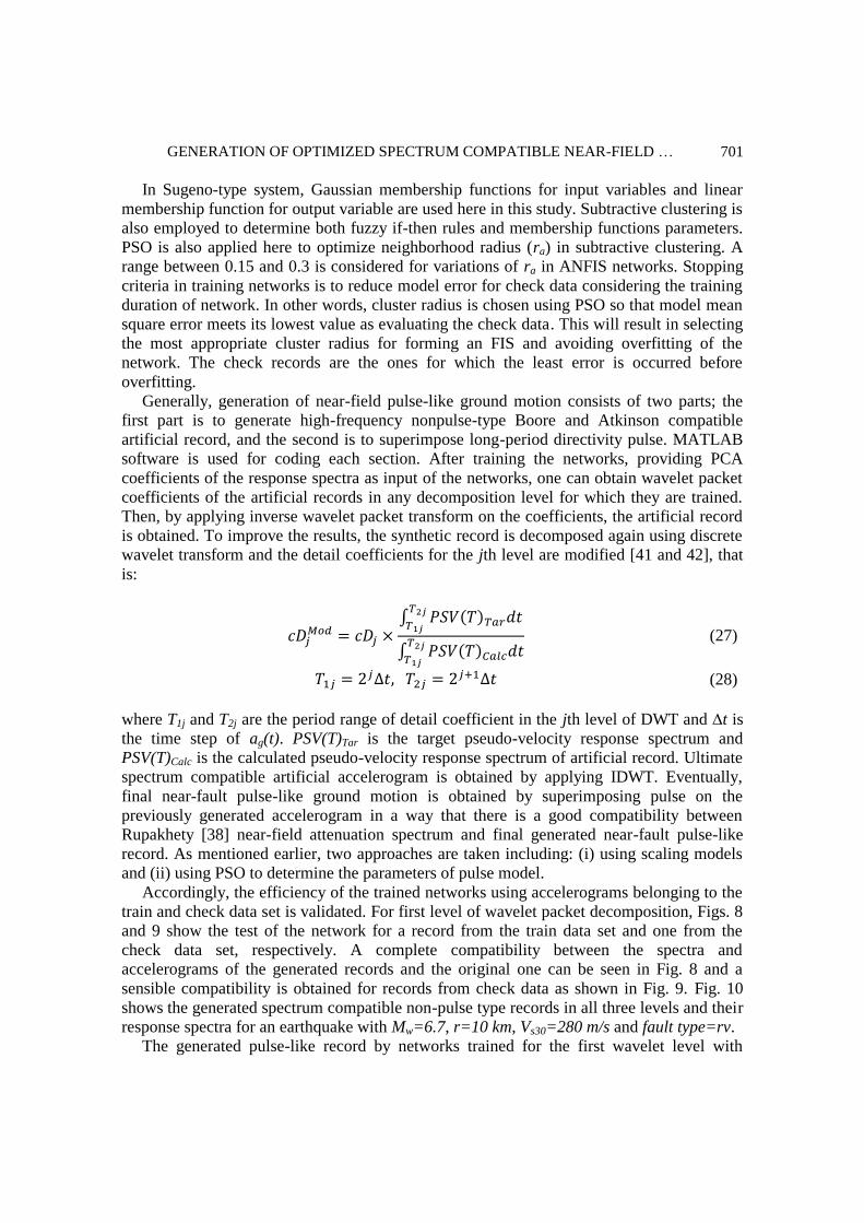
of pulses of Type 1 and 2, are shown in Figs. 12, 13, 14, 15 and 16.

5. CONCLUSIONS

In this study, an alternative method based on wavelet analysis, neuro-fuzzy networks, PSO

and PCA is developed to generated near-fault pulse-like ground motions. First, directivity

pulses, known as the most important characteristic of near-fault ground motions, are

extracted. It was noticed that the Boore and Atkinson [36] prediction model resembles the

spectra of the residual records, therefore, first nonpulse-type ground motions are simulated

using learning abilities of ANFIS networks and multi-resolution wavelet packet transform to

expand the relationship between PCA coefficients of the response spectra and each points of

wavelet packet coefficients. An illustrative example using 23 near-fault records was shown

in which good results of spectrum compatibility for the generated nonpulse-type records was

obtained. At the end, directivity pulse models were used to generate final near-fault pulse-

like ground motion which was compatible with Rupakhety near-fault model. Except for the

records and their response spectra, nothing else is needed in this method to produce near-

fault records.

Figure 8. Comparison of original and generated records belong to train set (1979 Imperial

Valley-06, Brawley Airport): (a) Records, (b) Response spectra

0 5 10 15 20 25 30-1

-0.6

-0.2

0.2

0.6

1

Acc

eler

atio

n (

1g

)

Original

0 5 10 15 20 25 30-1

-0.6

-0.2

0.2

0.6

1

Time (sec)

Artificial

Acc

eler

atio

n (

1g

)

(a)

10-2

10-1

100

101

10-2

10-1

100

Response spectra

Pse

ud

o-v

elo

city

(m

/s)

Period (sec)

Original record

Artificial record

(b)


Figure 9. Comparison of original and generated records belong to check data set (Whittier

Narrows-01 1987, LB - Orange Ave): (a) Records, (b) Response spectra

Fig. 10. (a) Generated non-pulse type ground motion for three levels, (b) Response spectra

Figure 11. (a) Generated pulse-like ground motion for level 1 using PSO and pulse Type 1, (b)

Response spectra

0 5 10 15 20 25 30-1.2-0.8-0.4

00.40.81.2

Acc

eler

atio

n (

1g

)

Original

0 5 10 15 20 25 30-1.2-0.8-0.4

00.40.81.2

Acc

eler

atio

n (

1g

)

Artificial

Time (sec)

(a)

10-2

10-1

100

101

10-2

10-1

100

Response spectra

Period (sec)

Pse

ud

o-v

elo

city

(m

/s)

Original record

Artificial record

(b)

0 10 20 30

-1

0

1

Artificial: L1

Acc

eler

atio

n (

1g

)

0 10 20 30

-1

0

1

Artificial: L2

Acc

eler

atio

n (

1g

)

0 10 20 30

-1

0

1

Artificial: L3

Acc

eler

atio

n (

1g

)

Time (sec)

(a)

10-2

10-1

100

101

10-2

10-1

100

Response spectra

Period (sec)

Pse

ud

o-v

elo

oci

ty (

m/s

2)

Boore and Atkinson

Artificial L1

Artificial L2

Artificial L3

(b)

0 10 20 30

-0.2

0

0.2

0.4

0.6

Vel

oci

ty (

m/s

)

Time (sec)

(a)

10-2

10-1

100

101

10-2

10-1

100

101

Period (sec)

Pse

udo-a

ccel

erati

on

(m

/s2)

Artificial pulse-like ground motion

Rupakhety prediction model

Boore and Atkinson prediction model

Artificial non-pulse like ground motion

(b)


Figure 12. (a) Generated pulse-like ground motion for level 1 using scaling models and pulse

Type 2, (b) Response spectra

Figure 13. (a) Generated pulse-like ground motion for level 2 using PSO and pulse Type 1, (b)

Response spectra





0 10 20 30-0.6

-0.4

-0.2

0

0.2

0.4

0.6V

elo

city

(m

/s)

Time (sec)

(a)

10-2

10-1

100

101

10-2

10-1

100

101

Period (sec)

Pse

udo-a

ccel

erati

on

(m

/s2)





(b)

0 10 20 30-0.4

-0.2

0

0.2

0.4

0.6

0.8

Vel

oci

ty (

m/s

)

Time (sec)

(a)

10-2

10-1

100

101

10-2

10-1

100

101

Period (sec)

Pse

udo-a

ccel

erati

on

(m

/s2)





(b)

0 10 20 30-0.6

-0.4

-0.2

0

0.2

0.4

0.6

Vel

oci

ty (

m/s

)

Time (sec)

(a)

10-2

10-1

100

101

10-2

10-1

100

101

Period (sec)

Pse

udo-a

ccel

erati

on

(m

/s2)





(b)

0 10 20 30

-0.2

0

0.2

0.4

0.6

Vel

oci

ty (

m/s

)

Time (sec)

(a)

10-2

10-1

100

101

10-2

10-1

100

101

Period (sec)

Pse

udo-a

ccel

erati

on

(m

/s2)





(b)


Figure 16. (a): Generated pulse-like ground motion for level 3 using PSO and pulse Type 2, (b):

Response spectra

REFERENCES

[1] Somerville PG, Smith NF, Graves RW, Abrahamson NA. Modification of empirical

strong ground motion attenuation relations to include the amplitude and duration effects

of rupture directivity, Seismol Res Letter 1997; 68(1): 199-222.

[2] Stewart JP, Chiou SJ, Bray JD, Graves RW, Somerville PG, Abrahamson NA. Ground

motion evaluation procedures for performance based design, Rpt. No. PEER-2001/09,

PEER Center, 2001.

[3] Ghaboussi J, Lin CJ. New method of generating spectrum compatible accelerograms

using neural networks, Earthq Eng Struct Dyn 1998; 27: 377-96.

[4] Lin CJ, Ghaboussi J. Generating multiple spectrum compatible accelerograms using

stochastic neural networks, Earthq Eng Struct Dyn 2001; 30: 1021-42.

[5] Lee SC, Han SW. Neural-network-based models for generating artificial earthquakes

and response spectra, Comput Struct 2002; 80: 1627-38.

[6] Rajasekaran S, Latha V, Lee SC. Generation of artificial earthquake motion records

using wavelets and principal component analysis, J Earthq Eng 2006; 10(5): 665-91.

[7] Suarez LE, Montejo LA. Generation of artificial earthquake via the wavelet transform,

Int J Solid Struct 2005; 42: 5905-19.

[8] Hancock J, Waston-Lamprey J, Abrahamson NA, Bommer JJ, Markatis A, Macoy E and

Mendis R. An improved method of matching response spectra of recorded earthquake

ground motion using wavelets, J Earthq Eng 2006; 10(special issue 1): 67-89.

[9] Kaveh A, Mahdavi VR. A new method for modification of ground motions using

wavelet transform and enhanced colliding bodies optimization, Appl Soft Comput 2016;

47: 357-69.

[10] Kaveh A, Mahdavi VR. Modification of ground motions using wavelet transform and

VPS algorithm, Eartq Struct 2017; 12(4): 389-95.

[11] Hall JF, Heaton TH, Halling MW, Wald DJ. Near-source ground motion and its effects

on flexible buildings, Earthq Spect 1995; 11(4): 569-605.

[12] Iwan WD. Drift spectrum: measure of demand for earthquakeground motions, J Struct

Eng ASCE 1997; 123(4): 397-404.

0 10 20 30-0.6

-0.4

-0.2

0

0.2

0.4

0.6V

elo

city

(m

/s)

Time (sec)

(a)

10-2

10-1

100

101

10-2

10-1

100

101

Period (sec)

Pse

udo-a

ccel

erati

on

(m

/s2)





(b)


[13] Makris N. Rigidity-plasticity-viscosity: can electrorheological dampers protect base-

isolated structures from near-source ground motions?, Earthq Eng Struct Dyn 1997;

26(5): 571-91.

[14] Anderson JC, Bertero VV, Bertero RD. Performance improvement of long period

building structures subjected to severe pulse-type ground motions, PEER Report,

University of California at Berkeley, California, 1999.

[15] Malhotra PK. Response of buildings to near-field pulse-like ground motions, Earthq

Eng Struct Dyn 1999; 28: 1309-26.

[16] Chopra AK, Chintanapakdee C. Comparing response of SDOF systems to near-fault and

far-fault earthquake motions in the context of spectral regions, Earthq Eng Struct Dyn

2001; 30: 1769-89.

[17] Pavlou EA, Constantinou MC. Response of elastic and inelastic structures with damping

systems to near-field and soft-soil ground motions, Eng Struct 2004; 26: 1217-30.

[18] Sehhati R, Rodriguez-Marek A, ElGawady M, Cofer WF. Effects of near-fault ground

motions and equivalent pulses on multi-story structures, Eng Struct 2011; 33: 767-79.

[19] Mavroeidis GP, Papageorgiou AS. A mathematical representation of near-fault ground

motions, Bulletin Seismolog Society America 2003; 93(3): 1099-1131.

[20] Li X, Zhu X. Study on equivalent velocity pulse of near-fault ground motions, ACTA

Seismolog Sinica 2004; 17(6): 697-706.

[21] Yushan Z, Yuxian H, Fengxin Z, Jianwen L, Caihong Y. Identification of acceleration

pulses in near-fault ground motion using the EMD method, Earthq Eng Eng Vibrat

2005; 4(2): 201-12.

[22] Tian Y, Yang Q, Lu M. Simulation method of near-fault pulse-type ground motion,

ACTA Seismolog Sinica 2007; 20(1): 80-7.

[23] Baker JW. Quantitative classification of near-fault ground motions using wavelet

analysis, Bulletin Seismolog Society America 2007; 97(5): 1486-1501.

[24] Fan J, Dong P. Simulation of artificial near-fault ground motions based on the S-

transform, Congress on Image and Signal Processing 2008, pp. 518-522.

[25] Nicknam A, Abbasnia R, Bozorgnasab M, Eslamian Y. Synthesizing Broadband Time-

Histories at Near Source Sites; Case Study, 2003 BamMw6.5 Earthquake, J Earthq Eng

2010; 14: 898-917.

[26] Yaghmaei-Sabegh S. Detection of pulse-like ground motions based on continues

wavelet transform, J Seismolo 2010; 14(4): 715-26.

[27] Ghodrati AG, Abdolahi Rad A, Aghajari S, Khanmohamadi Hazaveh N. Generation of

near-field artificial ground motions compatible with median-predicted spectra using

PSO-based neural network and wavelet analysis, Comput-Aided Civil Infrastruct Eng

2012; 27: 711-30.

[28] Tahghighi H. Simulation of strong ground motion using the stochastic method:

application and validation for near-fault region, J Earthq Eng 2012; 16: 1230-47.

[29] Mukhopadhyay S, Gupta VK. Directivity pulses in near-fault ground motions-I:

identification, extraction and modelling, Soil Dyn Earthq Eng 2013; 50: 1-15.

[30] MATLAB. Reference Guide, the Math Works Inc, 2002.

[31] Jang JSR. ANFIS: Adaptive-Network-based Fuzzy Inference Systems, IEEE Trans on

Syst Man Cybern 1993; 23(3): 665-85.

[32] MATLAB. Reference Guide, the Math Works Inc, 2014.


[33] Chiu SL. Fuzzy model identification based on cluster estimation, J Intelligent Fuzzy

Syst 1994; 2(3): 267-278.

[34] Kennedy J, Eberhart R. Particle swarm optimization, Proceedings of the IEEE

International Conference on Neural Networks 1995, pp. 1942-1948.

[35] Clerc M, Kennedy J. The particle swarm-explosion, stability, and convergence in a

multidimensional complex space, IEEE Transact Evolut Comput 2002; 6(1): 58-73.

[36] Boore D, Atkinson G. Ground-motion prediction equations for the average horizontal

component of PGA, PGV, and 5%-damped PSA at spectral periods between 0.01 s and

10.0 s, Earthq Spectra 2008; 24: 99-138.

[37] Baker JW. Identification of near-fault velocity pulses and prediction of resulting

response spectra, Geotechnical Earthquake Engineering and Soil Dynamics IV 2008,

Sacramento, CA, pp. 1-10.

[38] Rupakhety R, Sigurdsson SU, Papageorgiou AS, zigbjörnsson R. Quantification of

ground-motion parameters and response spectra in the near-fault region, Bull Earthq

Eng 2011; 9: 893-930.

[39] Mukhopadhyay S, Gupta VK. Directivity pulses in near-fault ground motions-II:

Estimation of pulse parameters, Soil Dyn Earthq Eng 2013; 50: 38-52.

[40] Trifunac MD, Brady AG. A study of the duration of strong earthquake ground motion,

Bull Seismolo Soc American 1975; 65: 581-626.

[41] Mukherjee S, Gupta K. Wavelet-based characterization of design ground motions,

Earthq Eng Struct Dyn 2002; 31: 1173-90.

[42] Mukherjee S, Gupta K. Wavelet-based generation of spectrum-compatible time-

histories, Soil Dyn Earthq Eng 2002; 22: 799-804.

APPENDIX

See Table A1.

Table A1: Near-fault records used in this study

# Event, Year, Station Mw

Joyner-

Boore

Dist. (km)

Vs30

(m/s) PI

Dominant

Fourier period

of pulse

Extracted

pulse

types

1 Imperial Valley-06, 1979, Agrarias 6.5 0.00 275 1.00 2.16 1

2 Imperial Valley-06, 1979, Brawley

Airport 6.5 8.54 209 0.87 3.72 - 5.85 2 and 2

3 Imperial Valley-06, 1979, EC County

Center FF 6.5 7.31 192 0.99 4.55 2

4 Imperial Valley-06, 1979, El Centro

Array #10 6.5 6.17 203 0.98 6.83 - 5.12 1 and 2


Array #3 6.5 10.79 163 1.00 5.12 1


Array #4 6.5 4.90 209 1.00 4.55 2


Array #5 6.5 1.76 206 1.00 4.10 2



Array #6 6.5 0.00 203 1.00 4.10 2

9 Imperial Valley-06, 1979, Holtville

Post Office 6.5 5.51 203 1.00 4.55 1

10 Westmorland, 1981, Parachute Test

Site 5.9 16.54 349 0.76 5.85 1

11 Taiwan SMART1(40), 1986,

SMART1 C00 6.3

274 0.82 1.52 1

12 Taiwan SMART1(40), 1986,

SMART1 M07 6.3

274 0.99 1.52 1

13 Whittier Narrows-01, 1987, Downey -

Co Maint Bldg 6.0 14.95 272 0.98 0.91 - 1.78 1 and 2

14 Whittier Narrows-01, 1987, LB -

Orange Ave 6.0 19.80 270 0.99 0.93 1

15 Superstition Hills-02, 1987, Parachute

Test Site 6.5 0.95 349 0.85 2.41 1

16 Loma Prieta, 1989, Gilroy Array #2 6.9 10.38 271 0.76 1.64 1

17 Erzican, Turkey, 1992, Erzincan 6.7 0.00 275 0.99 2.56 1

18 Landers, 1992, Barstow 7.3 34.86 371 0.98 8.19 1

19 Landers, 1992, Yermo Fire Station 7.3 23.62 354 1.00 7.45 1

20 Northridge-01, 1994, Newhall - W

Pico Canyon Rd. 6.7 2.11 286 0.99 3.15 2

21 Northridge-01, 1994, Sylmar -

Converter Sta 6.7 0.00 251 0.87 1.79 - 3.57 1 and 1

22 Northridge-01, 1994, Sylmar -

Converter Sta East 6.7 0.00 371 1.00 3.72 - 1.52 1 and 1

23 Kobe, Japan, 1995, Takatori 6.9 1.46 256 0.72 2.28 1

24 Northwest China-03, 1997, Jiashi 6.1

274 1.00 1.67 1

25 Chi-Chi, Taiwan-06, 1999, CHY101 6.3 34.55 259 0.70 2.56 1

generation of optimized spectrum compatible near …

Documents