generation reliability for isolated power sys- tems with...

Generation Reliabilityfor Isolated Power Sys-tems with Solar, Windand Hydro Generation

Jimmy Ehnberg

Department of Electric Power EngineeringCHALMERS UNIVERSITY OF TECHNOLOGY

Goteborg, Sweden 2003

THESIS FOR THE DEGREE OF LICENTIATE OF ENGINEERING

Generation Reliability for IsolatedPower Systems with Solar, Wind and

Hydro Generation

Jimmy Ehnberg

Department of Electric Power EngineeringCHALMERS UNIVERSITY OF TECHNOLOGY

Goteborg, Sweden 2003

Generation Reliability for Isolated Power Systemswith Solar, Wind and Hydro Generation

Jimmy Ehnberg

c© Jimmy Ehnberg, 2003.

Technical Report No. 478LISSN: 1651-4998

Department of Electric Power EngineeringCHALMERS UNIVERSITY OF TECHNOLOGYSE-412 96 GoteborgSwedenTelephone + 46 (0)31 772 1000

Chalmers Bibliotek, ReproserviceGoteborg, Sweden 2003

Abstract

This licentiate thesis deals with reliability issues for small isolated power systems. Thefocus is on power systems in remote areas based entirely on renewable energy sources.The sources investigated in this thesis are mainly solar and wind power and models forthese energy sources are presented.

The solar power model is based on the solar declination and cloud coverage. In addi-tion a Markov theory based model for simulating cloud coverage data is presented. Thewind power model is based on two Markov chains, one for low wind and one for highwind. Both the solar and the wind models use measurements as input but by usingnormalised wind speed measurements a more general wind speed model is obtained.There are still, but minor, needs for site-specific meteorological measurements.

The presented models of solar and wind power are together with some simpler modelsof hydro power, storage and loads used for case studies. Since the solar model is de-pendent on the location, a site in Africa is used. Timbuktu in Mali was chosen for itssubsahara climate and the fact that Mali is considered a developing country. Twelvecases were studied with combinations of solar, wind and hydro power both with andwithout storage possibilities.

A case study with only wind as power source has a higher overall availability thenone with only solar power. But since all the solar power is available during daytimethe availability is higher for solar power during daytime. By adding storage capabil-ity the overall availability will be higher for solar power because more efficient use ofthe storage. Combining the power sources with small hydro power (only 10% of totalmaximum load) the availability will be significantly increased. The hydro power willthen supply the load during low load hours.

A combination of all three power sources gives a high reliability because during thehigh daytime load all three sources are available and during nighttime both wind andhydro are available. The largest availability problems are during mornings and eveningswhen the load is high but the solar power has a low availability. This effect is seasondependent.

To be able to use exclusively renewable energy sources a combination of sources isneeded to secure the reliability of the supply.

Keywords: Renewable energy, Stochastic modelling, Generation reliability, Isolatedpower systems, Solar power, Wind power.

iii

Acknowledgement

First, I would like to thank Professor Math Bollen for initiating the project with AGSand for the support and encouragement. His support was always there and the “doorwas always open” in case of problems and short questions.

I will also thank Professor Stanislaw Gubanski and Assistant Professor Jorgen Blennowfor teaching me the basics of being a Ph.D student and Yuriy Serdyuk, room-mate, forsharing his experience in the field of academic work with me.

I would like to thank the Alliance of Global Sustainability (AGS) for their finan-cial support and Swedish Meteorological and Hydrological Institute (SMHI) and HansBergstrom at Uppsala University for providing meteorological data.

The colleagues at the department, for the help in different areas and making the de-partment a fun place to work, should also be acknowledged. Also other friends, outsidethe department, for their support in their own way.

Finally, I will acknowledge Susanna and my parents for their understanding, encour-agement and love throughout the project.

v

List of Publications

J.S.G. Ehnberg, M.H.J. Bollen, “Simulation of global solar radiation based on cloudobservations,” International Solar Energy Conference, Gothenburg, May 2003.

J.S.G. Ehnberg, M.H.J. Bollen, “Reliability of a small power system using solar powerand hydro,” Submitted to Electric Power Systems Research.

J.S.G. Ehnberg, M.H.J. Bollen, “Reliability of a small isolated power system in remoteareas based on wind power,” Submitted to Nordic Wind Power Conference, Gothen-burg, March 2004.

vii

Contents

Abstract iii

Acknowledgement v

List of Publications vii

1 Introduction 11.1 Isolated power systems . . . . . . . . . . . . . . . . . . . . . . . . . . . 11.2 Stochastic modelling of renewables . . . . . . . . . . . . . . . . . . . . 21.3 Aim of this study . . . . . . . . . . . . . . . . . . . . . . . . . . . . . . 21.4 Contents of this study . . . . . . . . . . . . . . . . . . . . . . . . . . . 2

2 Generation Reliability 52.1 Hierarchical levels . . . . . . . . . . . . . . . . . . . . . . . . . . . . . . 52.2 Level I reliability . . . . . . . . . . . . . . . . . . . . . . . . . . . . . . 52.3 Reliability quantifiers . . . . . . . . . . . . . . . . . . . . . . . . . . . . 62.4 Reliability assessment . . . . . . . . . . . . . . . . . . . . . . . . . . . . 7

2.4.1 Generation capacity outage table . . . . . . . . . . . . . . . . . 72.4.2 Frequency and duration method . . . . . . . . . . . . . . . . . . 82.4.3 Markov models . . . . . . . . . . . . . . . . . . . . . . . . . . . 92.4.4 Monte-Carlo simulation . . . . . . . . . . . . . . . . . . . . . . 12

2.5 Renewable Energy . . . . . . . . . . . . . . . . . . . . . . . . . . . . . 12

3 Power System Models 133.1 Sun power generation model . . . . . . . . . . . . . . . . . . . . . . . . 13

3.1.1 Definitions . . . . . . . . . . . . . . . . . . . . . . . . . . . . . . 143.1.2 Astronomical and Meteorological relationships . . . . . . . . . . 153.1.3 Results . . . . . . . . . . . . . . . . . . . . . . . . . . . . . . . . 173.1.4 Cloud simulations . . . . . . . . . . . . . . . . . . . . . . . . . . 203.1.5 Solar cells . . . . . . . . . . . . . . . . . . . . . . . . . . . . . . 25

3.2 Hydro power generation model . . . . . . . . . . . . . . . . . . . . . . . 283.3 Wind power generation model . . . . . . . . . . . . . . . . . . . . . . . 29

3.3.1 Obtaining the measured data . . . . . . . . . . . . . . . . . . . 303.3.2 Simulation using Markov Models . . . . . . . . . . . . . . . . . 313.3.3 Wind speed variations with height . . . . . . . . . . . . . . . . . 353.3.4 Wind Turbine . . . . . . . . . . . . . . . . . . . . . . . . . . . . 37

3.4 Load model . . . . . . . . . . . . . . . . . . . . . . . . . . . . . . . . . 383.5 Storage model . . . . . . . . . . . . . . . . . . . . . . . . . . . . . . . . 39

ix

3.5.1 Model used in this thesis . . . . . . . . . . . . . . . . . . . . . . 43

4 Case Study, Timbuktu 454.1 Solar power only . . . . . . . . . . . . . . . . . . . . . . . . . . . . . . 484.2 Solar power with ideal storage . . . . . . . . . . . . . . . . . . . . . . . 504.3 Solar and hydro power . . . . . . . . . . . . . . . . . . . . . . . . . . . 524.4 Solar and hydro power with ideal storage . . . . . . . . . . . . . . . . . 544.5 Wind power . . . . . . . . . . . . . . . . . . . . . . . . . . . . . . . . . 574.6 Wind power with ideal storage . . . . . . . . . . . . . . . . . . . . . . . 584.7 Solar and wind power . . . . . . . . . . . . . . . . . . . . . . . . . . . . 604.8 Solar and wind with ideal storage . . . . . . . . . . . . . . . . . . . . . 614.9 Wind and hydro power . . . . . . . . . . . . . . . . . . . . . . . . . . . 634.10 Wind and hydro power with ideal storage . . . . . . . . . . . . . . . . . 644.11 Solar, wind and hydro power . . . . . . . . . . . . . . . . . . . . . . . . 684.12 Solar, wind and hydro power with ideal storage . . . . . . . . . . . . . 714.13 Discussions of Case studies . . . . . . . . . . . . . . . . . . . . . . . . . 74

5 Conclusions 77

6 Future Work 79

References 81

x

Chapter 1

Introduction

1.1 Isolated power systems

The use of electric power has increased during the last centuries and almost anyoneneeds electricity. Despite the wide coverage of large power systems, all costumers arenot connected to a large power system. A small power system that is not connectedto a much larger grid is called an isolated power system.

Example of isolated power systems are

• Cars

• Planes

• Ships

• Oil platforms

• Small islands

• Isolated villages far from a well-developed transmission and distribution grid.

How to provide power for the different small isolated power system varies due to sur-rounding conditions. The traditional source of energy in remote areas is wood but thereare a shift to electric energy through diesel generators. The next, more environmentally-friendly, stage is introducing renewable sources like solar, wind and hydro power. Oneproblem with use of diesel generators are transportation of the fuel. This is a majorenvironmental hazard and high cost for a remote location.

A better solution is to use renewable energy sources: like solar, wind and hydro power.There are advantages and disadvantages of using renewables. The main advantages arethat the system is environmental-friendly and there are very limited transport costs.A disadvantage is the uncertainty in power supply, which gives a lower reliability ofthe system.

Renewables are in most cases used as a complement to a diesel generator or to a largegrid. The challenge however is to build a system with only renewables.

1

1.2 Stochastic modelling of renewables

Stochastic modelling of power sources is often done by assuming a constant genera-tion capacity (often maximal) with planned interruptions and stochastic distributionof unplanned interruptions [1]. This model is valid for generators in power stations likenuclear and with fossil fuel. The method may even be applied to large scale hydro in-stallation, albeit with some restrictions. For power stations that are dependent on themeteorological conditions this method is not applicable. Meteorologically dependentsources are e.g. solar and wind power.

The stochastic behavior of solar and wind power has a strong correlation with theweather. The amount of sunshine and the wind speed are not the only factors thataffect the performance of the sources. Important other factors for solar power aretemperature and shading [2], while for wind they are terrain, shading from other windturbines and air density [3]. The shading from other wind turbines only affects theenergy production in wind farms [4].

1.3 Aim of this study

The aim of this study is to gain understanding of renewable energy sources and interac-tions between sources. This will be done through development of stochastic models forrenewable energy that can be used in power system reliability studies. The emphasiswill be on the development of consistent models. The aim of case studies will be toprove the applicability of the models in the power system reliability studies.

Another issue is the need for meteorological data. We want models that can be appliedto remote villages e.g. in the Mali desert or in the mountains of Tibet, without theneed to do several years of measurements.

Other aims of this study are to indicate where more knowledge is needed and to func-tion as a preparation for future projects with a multi-disciplinary approach.

This study is a part of a larger study within the Alliance for Global Sustainability(AGS). The larger study is a cooperation between Chalmers (Goteborg), ETH (Zurich),MIT (Boston), University of Tokyo and Shanghai Jiao Tong University. The main aimis to study isolated rural distribution networks with a large penetration of renewablesources. The study includes not only reliability issues but also source-system interfaces,social acceptance, controls and stability aspects and studies of currently used facilitiesin China and Africa. Each university is responsible for a part of the project.

1.4 Contents of this study

In this section each chapter is introduced and reading instructions are given accordingto the author.

2

Chapter 2: Generation Reliability

In this chapter the subject “generation reliability” is introduced. The most commontechniques are discussed. Theories behind other methods used in the thesis are brieflyintroduced, such as Markov theory and Monte-Carlo simulation.

Chapter 3: Power System Models

This chapter presents the models used in this thesis.

A stochastic model of solar power based on cloud coverage observations and a methodfor simulating cloud coverage based on Markov theory are proposed. The section aboutsolar power also contains a short presentation of some conversion technologies for solarpower.

A model of hydro power is presented based on constant flow-of-river and a small reser-voir.

A stochastic model of wind power is presented based on two Markov chains for simu-lating low and high wind. The mean value can be adapted to the one that exists atthe investigated geographical location. The section about wind power also contains ashort presentation of the most common conversion technologies for wind power.

A model for the load is also presented. The load model is based on both industrial andresidential loads.

The chapter ends with some discussion regarding storage, both existing methods andfuture technologies and the model used in the case studies.

Chapter 4: Case Study, Timbuktu

In this chapter a case study is presented. Case study of Timbuktu in Africa is done withsolar and wind power and combinations with and without hydro power and storage.The chapter ends with a comparison between different configurations of power sources.

Chapter 5: Conclusions

In this chapter the conclusions of this project are presented.

Chapter 6: Future Works

In this chapter some future research issues are identified.

Reading instructions

The main chapter is the case study and the model chapter contains the models usedin the case study. Chapter two explains some techniques and conceptions used in themodel chapter and in the case study. The reader may want to start by reading thecase studies and use the other chapters as a resource base for further understanding ofthe models used.

3

Chapter 2

Generation Reliability

2.1 Hierarchical levels

Since a modern power system is complex, highly integrated and very large, even ad-vanced computers will have problem to handle all in one entry. Therefore reliabilitystudies of power systems are typically split into three so-called “hierarchical levels”:generation, transmission and distribution [1].

The generation reliability (HLI) is the ability of the generation capacity to supply theload of the system, while the second hierarchical level (HLII) is transmission systemand its ability to deliver the bulk supply. The third and lowest level (HLIII) is thecomplete system and its ability to supply individual consumers [1].

2.2 Level I reliability

The balance between load and generation is very basic in the operation of electricpower systems. The balance is shown in a systematic way in Figure 2.1. At anymoment in time generation and load should be equal, in accordance with the physicallaw of conservation of energy. This balance is the basis of the power-frequency controlin interconnected power systems. Also for reliability assessment do we use this balancebetween generation and load but in a slightly different way. The load is compared withthe so-called “generation capacity”. The generation capacity is the sum of the powerthat can be produces by all generator units that are available to produce electricalenergy. These units do not have to be operational but they should have the potentialto be operational.

Generator units may be unavailable due to failures, this is called “forced unavailability”,or due to preventive maintenance, this is called “planned unavailability”. Both typesof unavailability may be treated stochastically, but the planned unavailability is oftentreated deterministically. The uncertainty in the generation capacity is then only dueto failures (outages) of generator units.

5

PSfrag replacements

G G

G

G

G

Load

Load Load

Load

Load

PowerSystem

Figure 2.1: Model for generation reliability calculations.

2.3 Reliability quantifiers

In reliability calculations some quantifiers are normally used. Some of them are pre-sented here according to the hierarchical level for which they are normally used [1].

Generation

LOLP (Loss Of Load Probability) = risk/probability that the load exceeds the gen-eration capacity for a certain mix of generation and a certain load. Basic calculationis comparing the total generation (with its uncertainties due to failures/outages) withthe annual peak load. This gives the probability that the maximum load cannot besupplied. Scheduled outages are typically not considered as maintenance is tradition-ally scheduled away from the annual peak.

LOLE (Loss Of Load Expectancy) = how much load that is lost, calculated over anumber of short time intervals. For example daily peak loads over one year, or hourlyloads during one year. Planned unavailability has to be considered in such a study.

Transmission

ELL (Expected load losses) = is the load that is expected to be lost. The value of ELLis often expressed in MW.

For HLII studies are also often LOLE used.

6

Distribution

SAIFI (System average interruption frequency index) = is the average interruptionfrequency per costumer. It is calculated as the ratio between total number of costumerinterruptions and the total number of costumers.

SAIDI (System average interruption duration index) = is the average duration of aninterruption per costumer. It is calculated as the ratio between the total time of cos-tumers interruption duration and the total number of costumers.

ASAI (Average service availability index) and ASUI Average service unavailabilityindex) = are the average time when the system is in service. They are calculated asthe ration between costumers hours of availability/unavailability and hours of demand.

AENS (Average energy not supplied index)= is the average amount of energy that arenot supplied and ACCI (average customer curtailment index) = are per costumer.

ENS (Energy not supplied index) = Is the power thatis missing supplied the load.

This thesis

In this thesis the terms availability and unavailability are used. Availability can beseen as the probability that the load will be supplied at an arbitrary chosen time. It isclose to the LOLP but annual peak load is not considered. Unavailability is one minusthe availability.

2.4 Reliability assessment

2.4.1 Generation capacity outage table

One of the most commonly used methods of determining the required generation forLOLE calculations is the generation capacity outage table [1]. If all units in a systemwere considered identical, but that is highly unlikely, an approach based on the bino-mial distribution could be used. The generation capacity outage table is based on theindependent behavior of the different units were each has its own unavailability.

To illustrate this a simple numeric example is shown in Table 2.1. Consider a systemwith three units, two 4 MW and one smaller at 3 MW. The two 4 MW units have anavailability of 0.97 while the 3 MW is more recently installed and has an availabilityof 0.98.

7

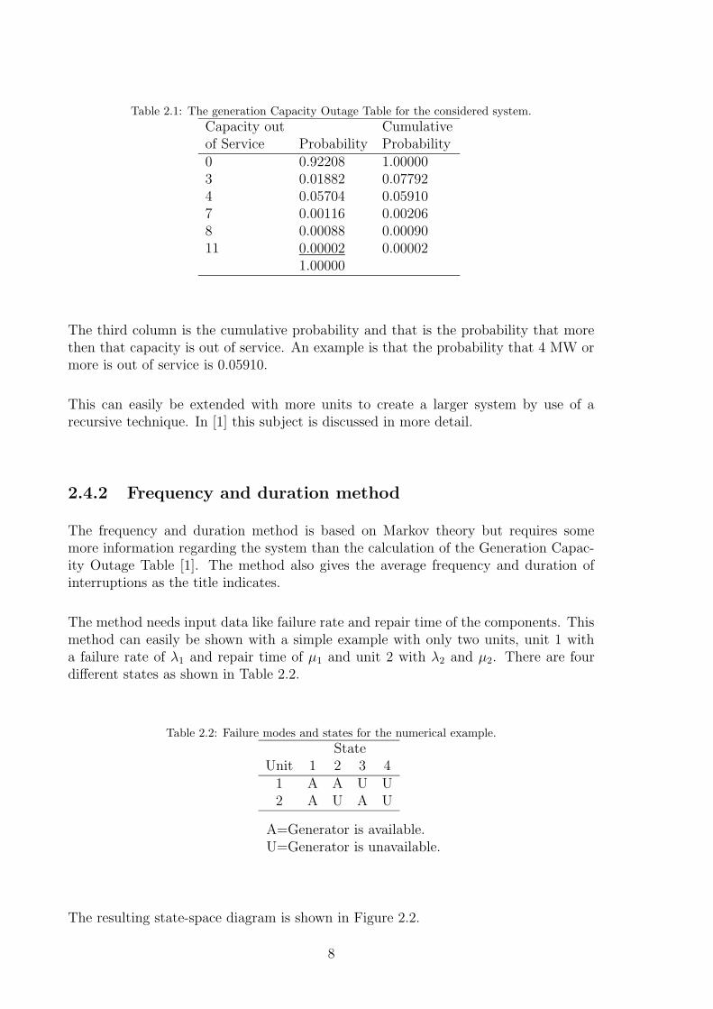
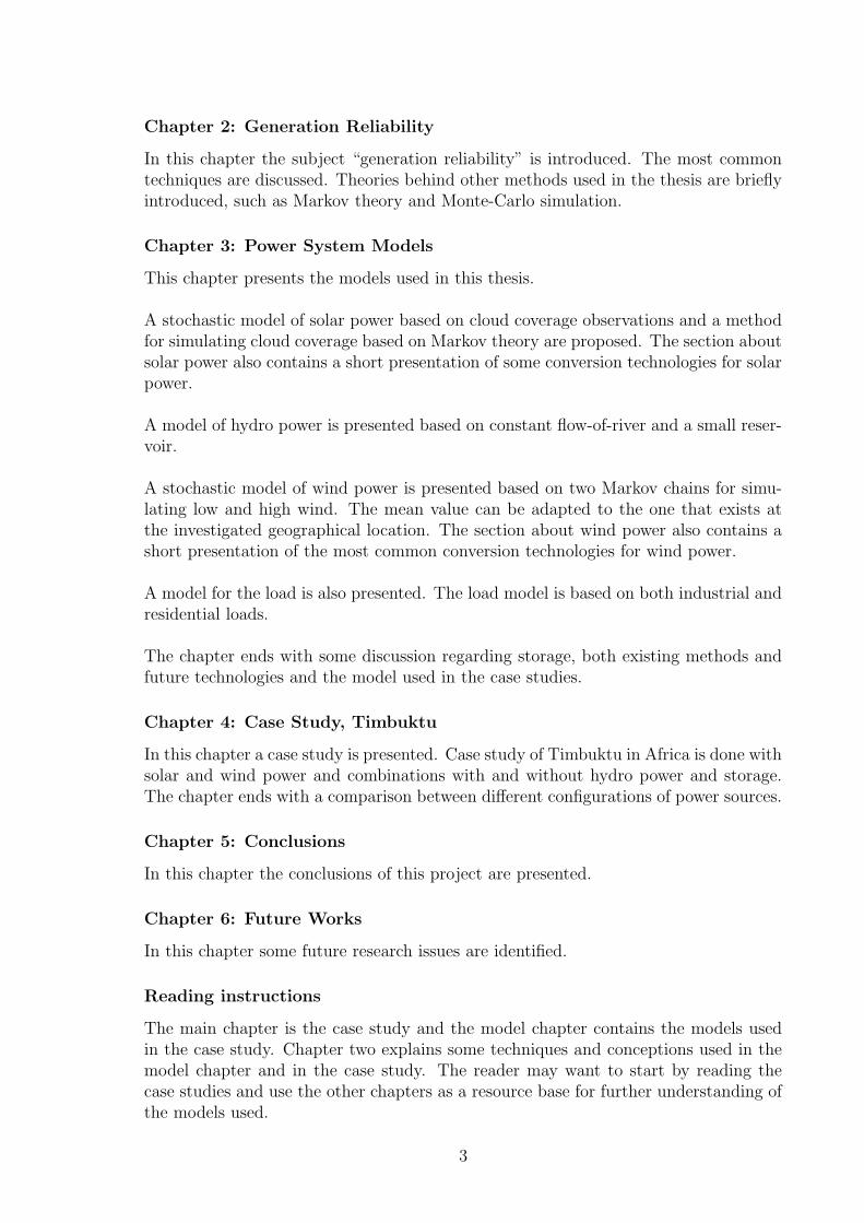
Table 2.1: The generation Capacity Outage Table for the considered system.

Capacity out Cumulativeof Service Probability Probability0 0.92208 1.000003 0.01882 0.077924 0.05704 0.059107 0.00116 0.002068 0.00088 0.0009011 0.00002 0.00002

1.00000

The third column is the cumulative probability and that is the probability that morethen that capacity is out of service. An example is that the probability that 4 MW ormore is out of service is 0.05910.

This can easily be extended with more units to create a larger system by use of arecursive technique. In [1] this subject is discussed in more detail.

2.4.2 Frequency and duration method

The frequency and duration method is based on Markov theory but requires somemore information regarding the system than the calculation of the Generation Capac-ity Outage Table [1]. The method also gives the average frequency and duration ofinterruptions as the title indicates.

The method needs input data like failure rate and repair time of the components. Thismethod can easily be shown with a simple example with only two units, unit 1 witha failure rate of λ1 and repair time of µ1 and unit 2 with λ2 and µ2. There are fourdifferent states as shown in Table 2.2.

Table 2.2: Failure modes and states for the numerical example.

StateUnit 1 2 3 41 A A U U2 A U A U

A=Generator is available.U=Generator is unavailable.

The resulting state-space diagram is shown in Figure 2.2.

8

PSfrag replacements

1 2

3 4λ1

λ1

µ1

µ1

λ2λ2 µ2µ2

Figure 2.2: State-space diagram for the example.

By using this methods and theory of asymptotic solution of a Markov model frequencyand duration may be calculated [5].

2.4.3 Markov models

The theory behind Markov chains and Markov processes is well know and are wellexplained in literature e.g. [5, 6, 7]. In this chapter is first the discrete Markov the-ory with finite states is introduced and then the continuous Markov theory with finitestates. Markov theory is often used in reliability calculation not only in power systemsbut also in e.g. computer science or telecommunication (Theory of Queueing). Markovtheory is also used for modelling stochastic behaviors like the models presented in thisthesis.

In Equation 2.1 the Markov property is shown. The property is the fundamentalequation in the Markov theory. A stochastic process that satisfies the Markov propertyis called a Markov process. The meaning of the Markov property is that the followingvalue in the stochastic process is only dependent on the current value.

P (Xn+1 = ij|Xn = in, Xn−1 = in−1, . . . , X0 = i0) = P (Xn+1 = ij|Xn = in) (2.1)

where Xn, n is an non-negative integer, is a discrete stochastic process with non-negative values and i0 to in and ij are values of that process.

Discrete Markov

In Equation 2.2 the definition of the transition probability is shown. The transitionprobability (pij) is the probability that the next value will be j if the current value isi.

P (Xn+1 = j|Xn = i) = pij (2.2)

The sum of the transition probabilities from a state is one, Equation 2.3 because therealways has to come a next value that has to be something. The next value may be

9

the same value if the transition probability, pii, is non-zero. For an absorbing state thetransition probability pii is one; it will never leave the state.

k∑

j=1

pij = 1 (2.3)

The transition probabilities can be summarized into a matrix (P ), the so-called tran-sition probability matrix. An example of a transition probability matrix can be seenin Equation 2.4.

P =

p00 p01 p02

p10 p11 p12

p20 p21 p22

(2.4)

If the transition probability is dependent on time, see Equation 2.5, the process iscalled non-homogenous or non-stationary. In the models in this thesis only homogenousor stationary process are used and time or other dependencies are modelled throughchanges between homogenous processes.

P (Xn+1 = j|Xn = i) = pij(n) (2.5)

A Markov process is often shown graphically in the form of a state-space diagram. Inthe state-space diagram each state is represented by a node and all non-zero transitionprobabilities are marked as a transition between the nodes. A state-space diagram fora three state process is shown in Figure 2.3. The corresponding transition probabilitymatrix is given in Equation 2.4. All the transition probabilities do not have to benon-zero.PSfrag replacements

p00

p10

p01

p11

p02

p20

p12

p21 p22

Figure 2.3: A state-space diagram for a three state system.

Continuous Markov

There is not a big difference between the discrete and the continuous Markov model.In the discrete there has to a transition inside the chain (could be to the same state)while in the continuous Markov model the time until the next transition is stochastic.

A state-space diagram for a three state system can be seen in Figure 2.2. That systemwill give a matrix, as in Equation 2.6.

10

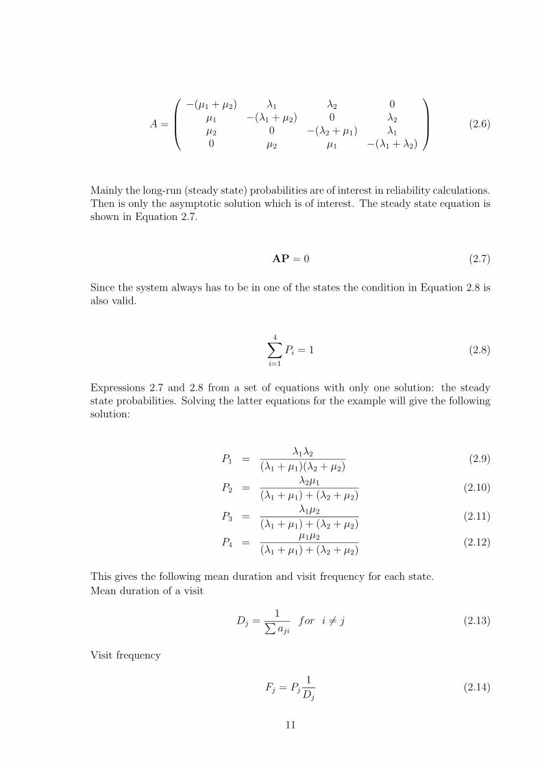
A =

−(µ1 + µ2) λ1 λ2 0µ1 −(λ1 + µ2) 0 λ2

µ2 0 −(λ2 + µ1) λ1

0 µ2 µ1 −(λ1 + λ2)

(2.6)

Mainly the long-run (steady state) probabilities are of interest in reliability calculations.Then is only the asymptotic solution which is of interest. The steady state equation isshown in Equation 2.7.

AP = 0 (2.7)

Since the system always has to be in one of the states the condition in Equation 2.8 isalso valid.

4∑

i=1

Pi = 1 (2.8)

Expressions 2.7 and 2.8 from a set of equations with only one solution: the steadystate probabilities. Solving the latter equations for the example will give the followingsolution:

P1 =λ1λ2

(λ1 + µ1)(λ2 + µ2)(2.9)

P2 =λ2µ1

(λ1 + µ1) + (λ2 + µ2)(2.10)

P3 =λ1µ2

(λ1 + µ1) + (λ2 + µ2)(2.11)

P4 =µ1µ2

(λ1 + µ1) + (λ2 + µ2)(2.12)

This gives the following mean duration and visit frequency for each state.

Mean duration of a visit

Dj =1

∑

ajifor i 6= j (2.13)

Visit frequency

Fj = Pj1

Dj

(2.14)

11

2.4.4 Monte-Carlo simulation

Evaluation techniques are of two main types: analytical and simulation. Using analyti-cal evaluation techniques demands mathematical models that describe everything. Forcomplex systems with a large dependencies the evaluation is not solvable analytically.By using simulation techniques, like Monte-Carlo, even larger complex systems can besolved. The Monte-Carlo methods, described in [5, 8, 9] are quite computer extensivebut have some other advantages. The main advantage is handle of both deterministicand stochastic models and dependencies. The simulation can include almost anythingthat effects the system such as weather variations, human errors, planned shutdownsand interactions with other systems. Differences in the models due to the differentexternal factors can easily be counted for. An example of a complex dependency inelectric power systems is the following. The failure of a component (e.g. a transmissionline or a generator) will lead to higher loading of some of the remaining components.If the loading gets too high this will lead to an increased failure rate of these compo-nents. As many large-scale blackouts are due to multiple failures, such dependenciesare important to consider in a reliability study.

The main idea with the Monte-Carlo method is the simulation of realistic or “typical”simulations. By repeating the “typical” simulations the resulting distribution of anystochastic variable can be determined. The more repetitions the higher accuracy anda high amount of the repetitions is especially needed for rare events [5].

The Monte-Carlo methods are often used in complex mathematical calculations, stochas-tic processes simulations, medical statistics, engineering system analysis and reliabilitycalculations [8].

For further studies of Monte-Carlo methods [9] is recommended.

2.5 Renewable Energy

The generation capacity now contains a third term (next to forced and planned un-availability): the fluctuations in the availability of the energy source. Such studies havebeen done already for large hydro installations, where the water level in the reservoirdepends on the amount of rain or snow over the previous year or so. With wind andsolar power the fluctuations affect the generation capacity even more.

The fluctuations in wind power are dependent on various non-human-controlled fac-tors, e.g. different meteorological conditions. Some factors that affect solar power, thatare also non-human-controlled, are time of the day, day of the year, water content inthe air and cloud coverage.

When use of renewables it is important to investigate the individual potential in eachkind of source get the maximum out of the sources. This will be discussed in moredetail in the next chapter.

12

Chapter 3

Power System Models

To be able to do reliability calculations of isolated power systems are models neededfor various components of the system. The models presented in this chapter are:

• Sun power generation model

• Water power generation model

• Wind power generation model

• Load model

• Storage model

The emphasis of the research has been on modelling solar and wind power. Thereforesimpler models has been taken for the other components.

3.1 Sun power generation model

In this section a model for simulating six-minute mean values of global solar radia-tion without any geographical restrictions is proposed and discussed. This model onlyuses the geographical coordinates of the location and cloud coverage data as input. Amethod of generating cloud coverage data by using a discrete Markov model is alsoproposed.

Several models have been proposed for generation of global radiation. The random na-ture of global solar radiation is included in all proposals, but the way of implementingthis in a model varies significantly. In [10, 11, 12] they model daily global solar radia-tion (thus the yearly variations) but a higher resolution of the simulation is needed forphotovoltaic power generation in an autonomous electric power system. Such modelwould be applicable in a system with a storage capability higher than the daily loaddemand. The model of [10, 12] requires several years of solar radiation measurements,which are for most locations not available. The model proposed by [11] is adapted forclear sky conditions but the authors mentioned the importance of the cloud coverage.In [13] hourly radiation have been modelled but the model could be difficult to applydue to the data requirements. Monthly average values of global radiation are neededwhich can only be obtained from long time measurements. Another model is proposedin [14] the problem with the input of the model remains. A location-dependent fac-tor is used which depends on the probability distribution of the solar radiation. Thismodel can again only be used when a large amount of solar radiation data is available.

13

Outside the atmosphere the solar radiation can accurately be determined [15] and theatmosphere will induce the randomness [13]. The transmittivity of solar radiation inthe atmosphere depends on various factors, e.g. humidity, air pressure and cloud type.A factor that has a great impact on the transmissivity is the cloud coverage [11, 16].By assuming a deterministic relation between cloud coverage and hourly global solarradiation, the need for measurement of the latter disappears. Cloud observations canbe used because of the simplicity of measuring, no expensive equipment is needed. Thelevel of cloudiness is expressed in Oktas which describes how many eight parts of thesky that are covered with clouds [17]. By combining the solar radiation model witha model of simulating cloud coverage the simulation method could be even more suit-able. The solar radiation distribution is expected to be similar in areas with similarclimatological conditions [14]. That means that this method could be used when cloudobservations are available for an area with similar climatological conditions. In reliabil-ity simulations for power systems without storage capacity, simulation data with higherresolution than one hour is needed in some cases. This is the case when short-durationinterruptions (less then one half hour) are a concern.

3.1.1 Definitions

Oktas The integer number of eighth parts of the sky which iscovered with clouds.

Solar declination angle, [δs] The angle between the equator and the center of sun tocenter of earth line, see figure 3.1.

Elevation angle, [ψ] The angle between the sun and the horizon.

UTC Coordinated Universal Time, the reference time,other names are GMT (Greenwich Mean Time) andZulu Z Time.

Global radiation The total radiation to the earth include reflections fromthe clouds, positive towards the center of earth.

Net income radiation The direct radiation from the sun.

14

Center of the sun to

Center of earth

Equator

North Pole

Figure 3.1: The solar declination angle [δs].

3.1.2 Astronomical and Meteorological relationships

The model consists of two parts, one deterministic and one stochastic. The determinis-tic part contains the astronomical effects while the meteorological effects are stochastic.

Astronomical effects are due to the earth orbiting around the sun and the rotationof the earth around its axis. The seasonal and daily variations can be described byequation 3.1 and 3.2 [15].

The equation for the seasonal effects 3.1, is an approximation under the assumptionof circular orbit of the earth around the sun. This assumption is allowed because theexcentricity is only 0.07 and the results are only used in stochastic ways. Equation 3.2describes the daily effects and is dependent on the geographical location.

δs ≈ Φr cos

[

C(d− dr)

dy

]

(3.1)

sinψ = sinφ sin δs

− cosφ cos δs cos

(

CtUTCtd

− λe

)

(3.2)

Where:

δs Solar declination angle, [rad]Φr The tilt of the earth‘s axis relative the orbital plane of the earth around the sun,

Φr = 0.409 [rad]C C = 2π, [rad]d Day of the year, [days]dr The day of the year at summer solstice, 173 (22 June) for non-leap years, [days]dy Total number of days in one year, [days]φ Latitude of the location [rad]λe Longitude of the location [rad]

The adjustment to local time from Coordinated Universal Time (UTC) is needed whenthe model should be used for reliability calculations and then combined with loads.

15

Loads have often a high correlation with time and therefor it is necessary to work withlocal time.

The randomness in this simulation model for global solar radiation is introduced in themeteorological part of the model. The importance of the randomness in the atmosphereis also discussed in [13]. An empirically determined relationship between the globalsolar radiation and the cloud coverage, equation 3.3 was obtained by the authors of[16], after many years of cloud observations, solar elevation measurements and globalsolar radiation measurements. The obtained relationship reads as follows:

S =

[

a0(N) + a1(N) sinψ + a3(N) sin3 ψ − L(N)

a(N)

]

(3.3)

S is the global solar radiation; the values of the constants L(N), a(N) and ai, i = 0, 1, 3in equation 3.3 are given in Table 3.1.

Table 3.1: The empiric determined coefficients for (3.3)

N a0 a1 a3 a L0 -112.6 653.2 174.0 0.73 -95.01 -112.6 686.5 120.9 0.72 -89.22 -107.3 650.2 127.1 0.72 -78.23 -97.8 608.3 110.6 0.72 -67.44 -85.1 552.0 106.3 0.72 -57.15 -77.1 511.5 58.5 0.70 -45.76 -71.2 495.4 -37.9 0.70 -33.27 -31.8 287.5 94.0 0.69 -16.58 -13.7 154.2 64.9 0.69 -4.3

In figure 3.2 the global solar radiation is presented as a function of the solar elevationangle for the nine possible values of cloud coverage. Note that even for a fully cloudedsky, a non-negligible part of the solar radiation reaches the solar panel (about 25%).

0 0.2 0.4 0.6 0.8 1−200

0

200

400

600

800

1000

1200

Sine of Solar Elevation Angle

Glo

bal S

olar

Rad

iatio

n [W

/m2 ]

0 1 2 3

4

5

6

7

8

Figure 3.2: The relationship between global solar radiation and solar elevation angle for different cloudcoverage. The number represents the cloud coverage level.

16

If the global radiation is below zero in 3.3 it should be set to zero according to equation3.4. If the radiation is negative it is from the surface of the earth upwards. Thisradiation has another frequency spectrum and will not generate any power from solarpanels. This situation will occur during night time and for low elevation angles.

if ψi < 0 or Si < 0 then Si = 0 ∀ i (3.4)

By examining global solar radiation measurements it can be seen that the radiationvaries within a one-hour period. This phenomena could be simulated by introducing astatistically varying term according to equation 3.5. This statistical term (ε) proposedto have the same distribution as the short duration variations seen in the measurements.

Sstat = S + ε (3.5)

The statistically varying term can be estimated through cross validation, the so-called”hold out method” proposed by [18]. The deviation from the hourly mean values forday time can be fitted to a normal distribution and the mean value and the standarddeviation can be estimated. The mean value of the deviation was estimated to zeroand the standard deviation to 40 W/m2 for a set of data obtained at Save Airport,close to Goteborg.

3.1.3 Results

To show some result of the global solar power model measured data obtained at SaveAirport (57.72 ◦N, 11.97 ◦E), close to Goteborg, was used. The data series consists ofsix-minute mean values of the global solar radiation and cloud coverage every threehour for 27 year. Hourly values of the cloud coverage were obtained through linear in-terpolation. The interpolated values were rounded to the nearest integer to correspondto a cloud coverage value.

To be able to see the difference between the different oktas, the solar radiation duringa whole year has been calculated with a constant oktas. The maximum value, of thesolar radiation for each day is displayed for each oktas in figure 3.3.

17

0 50 100 150 200 250 300 3500

200

400

600

800

1000

1200

Max

dai

ly g

loba

lradi

atio

n [W

/m2 ]

Time [days]

Oktas 0Oktas 1Oktas 2Oktas 3Oktas 4Oktas 5Oktas 6Oktas 7Oktas 8

Figure 3.3: Global solar radiation during one year for different oktas.

Figure 3.4 shows the maximum value of global solar radiation each day during one year,as measured at Save airport in Goteborg. As expected, the measured curve fluctuatesbetween the curve for oktas 0 (no clouds) and oktas 8 (fully clouded) in figure 3.3.

0 50 100 150 200 250 300 3500

100

200

300

400

500

600

700

800

900

Day of the year

Dai

ly m

axim

um o

f glo

bal s

olar

rad

iatio

n [W

/m2 ]

Figure 3.4: Calculation of the solar radiation for a year in Goteborg.

In figure 3.5 the global solar radiation, both measured and calculated, are shown for afew days in February. The calculated values where obtained by applying equation 3.3to the interpolated 1-hour values of the observed cloud coverage.

18

49 50 51 52 53 54 55 56 57 58−50

0

50

100

150

200

250

300

350

400

Time [days]

Glo

bal r

adita

ion

in G

öteb

org

1998

[W/m

2 ]

MeasuredCalculated

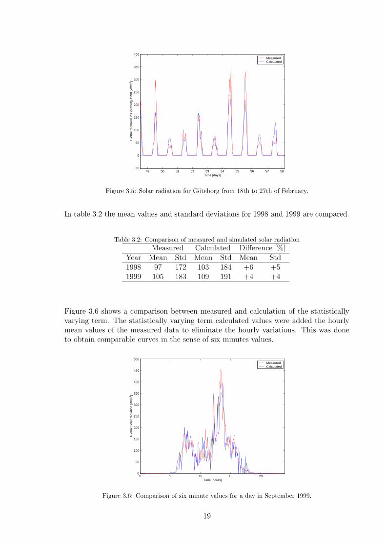
Figure 3.5: Solar radiation for Goteborg from 18th to 27th of February.

In table 3.2 the mean values and standard deviations for 1998 and 1999 are compared.

Table 3.2: Comparison of measured and simulated solar radiation

Measured Calculated Difference [%]Year Mean Std Mean Std Mean Std1998 97 172 103 184 +6 +51999 105 183 109 191 +4 +4

Figure 3.6 shows a comparison between measured and calculation of the statisticallyvarying term. The statistically varying term calculated values were added the hourlymean values of the measured data to eliminate the hourly variations. This was doneto obtain comparable curves in the sense of six minutes values.

0 5 10 15 200

50

100

150

200

250

300

350

400

450

500

Time [hours]

Glo

bal S

olar

rad

iatio

n [W

/m2 ]

MeasuredCalculated

Figure 3.6: Comparison of six minute values for a day in September 1999.

19

3.1.4 Cloud simulations

To make the model less dependent on observed cloud coverage data and thereby makeit more available for power system reliability calculations a model for simulate cloudcoverage data is developed. To use simulation techniques like Monte-Carlo many yearsof global solar radiation data is needed to get some statistic certainties. A Markovmodel is proposed to generate cloud coverage data from which global solar radiationcan be obtained. A Markov model was chosen because of its easiness and whereasit still allows dependencies to be accounted for. The transition probabilities in theMarkov model were obtained from measured values in the perhaps most intuitive way:

λij =fij

Σ8k=0

fik(3.6)

Where:

λij Is the estimated transitions probabilityfij The number of transitions from cloud coverage level i to level jfik The number of transitions from cloud coverage level i to level k

By using 27 years of cloud coverage data the transition probabilities could be deter-mined. The results are shown in matrix form below.

Λ =1

100

54 22 7.1 4.7 2.7 2.3 1.7 2.6 2.616 46 14 9.1 4.3 3.7 3.2 3.0 1.57.0 25 23 15 8.8 7.2 6.2 5.4 2.23.8 13 18 20 13 11 9.0 9.1 3.42.2 8.5 12 16 16 14 13 13 4.21.5 5.1 8.1 12 13 17 19 18 6.21.0 3.0 5.2 7.4 9.5 14 22 28 9.50.6 2.0 2.3 3.0 3.9 6.3 11 50 200.5 0.7 0.8 1.1 1.3 2.0 3.8 14 76

(3.7)

This way of simulating will generate cloud coverage data with the same time step asthe data used for input. The data used for this model have a time step of three hourswhich means that if this model is used it will generate simulated cloud coverage datawith a time step of three hours.

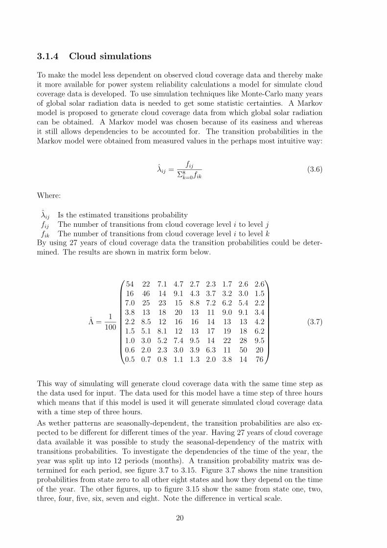
As wether patterns are seasonally-dependent, the transition probabilities are also ex-pected to be different for different times of the year. Having 27 years of cloud coveragedata available it was possible to study the seasonal-dependency of the matrix withtransitions probabilities. To investigate the dependencies of the time of the year, theyear was split up into 12 periods (months). A transition probability matrix was de-termined for each period, see figure 3.7 to 3.15. Figure 3.7 shows the nine transitionprobabilities from state zero to all other eight states and how they depend on the timeof the year. The other figures, up to figure 3.15 show the same from state one, two,three, four, five, six, seven and eight. Note the difference in vertical scale.

20

Jan Feb Mar Apr May Jun Jul Aug Sep Okt Nov Dec0

0.1

0.2

0.3

0.4

0.5

0.6

0.7

Time of the year

Tra

nsiti

ons

prob

abili

ties

to 0to 1to 2to 3to 4to 5to 6to 7to 8

Figure 3.7: The variations of the transition probabilities, from state 0, over a year.


0.1

0.2

0.3

0.4

0.5

0.6

0.7

Time of the year

Tra

nsiti

ons

prob

abili

ties




0.05

0.1

0.15

0.2

0.25

0.3

0.35

Time of the year

Tra

nsiti

ons

prob

abili

ties



21


0.05

0.1

0.15

0.2

0.25

Time of the year

Tra

nsiti

ons

prob

abili

ties




0.05

0.1

0.15

0.2

0.25

Time of the year

Tra

nsiti

ons

prob

abili

ties



22


0.05

0.1

0.15

0.2

0.25

0.3

0.35

Time of the year

Tra

nsiti

ons

prob

abili

ties




0.05

0.1

0.15

0.2

0.25

0.3

0.35

Time of the year

Tra

nsiti

ons

prob

abili

ties




0.1

0.2

0.3

0.4

0.5

0.6

0.7

Time of the year

Tra

nsiti

ons

prob

abili

ties



23


0.1

0.2

0.3

0.4

0.5

0.6

0.7

0.8

0.9

Time of the year

Tra

nsiti

ons

prob

abili

ties



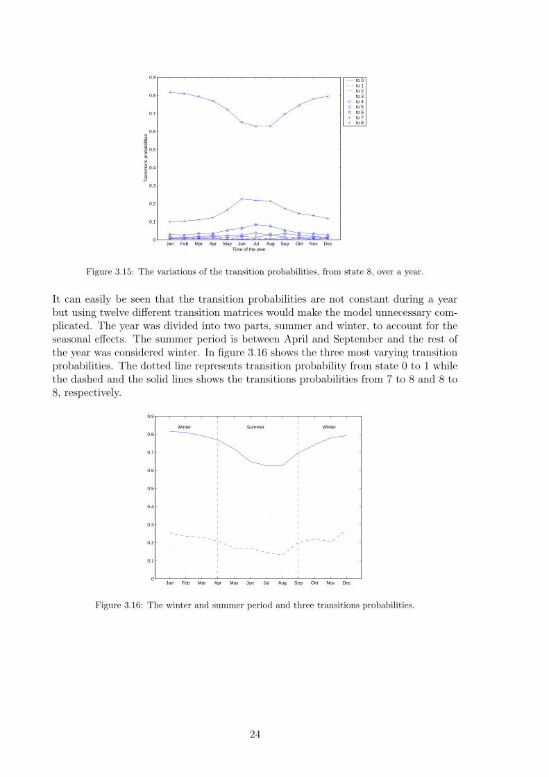
It can easily be seen that the transition probabilities are not constant during a yearbut using twelve different transition matrices would make the model unnecessary com-plicated. The year was divided into two parts, summer and winter, to account for theseasonal effects. The summer period is between April and September and the rest ofthe year was considered winter. In figure 3.16 shows the three most varying transitionprobabilities. The dotted line represents transition probability from state 0 to 1 whilethe dashed and the solid lines shows the transitions probabilities from 7 to 8 and 8 to8, respectively.


0.1

0.2

0.3

0.4

0.5

0.6

0.7

0.8

0.9

Winter Summer Winter

Figure 3.16: The winter and summer period and three transitions probabilities.

24

The resulting transition probabilities are for the summer period:

Λs =1

100

49 29 8.41 4.5 2.3 2.4 13 2.0 1.312 49 15 9.4 4.5 3.3 2.7 2.1 0.854.9 25 26 17 9.3 7.4 5.3 4.3 1.32.5 13 20 23 14 11 8.6 7.1 2.20.93 7.8 12 18 18 16 14 10 2.90.89 4.1 7.9 13 15 20 19 16 4.20.57 2.0 4.7 8.2 11 17 24 26 7.00.27 1.7 2.3 3.6 4.3 8.1 14 49 170.26 0.50 0.78 1.2 1.7 2.7 5.5 18 70

(3.8)

and for the winter period:

Λw =1

100

57 18 6.3 4.8 3.0 2.2 2.0 3.0 3.620 40 12 8.6 4.1 4.2 4.0 4.6 2.511 24 18 13 8.0 6.8 7.9 7.5 3.76.2 15 14 15 11 10 10 13 5.84.6 10 12 12 13 11 13 18 6.72.8 7.1 8.3 11 8.9 13 17 22 101.6 4.6 6.2 6.3 7.7 10 20 30 130.91 2.3 2.3 2.5 3.5 4.6 8.6 52 230.57 0.79 0.82 1.0 1.2 1.7 3.0 12 79

(3.9)

The method of using two matrices, summer and winter, is used for the reliabilitycalculations in this thesis.

3.1.5 Solar cells

There are today many different techniques of convert solar radiation to electric energy.In this chapter a selection of techniques of solar cells are presented [19].

Silicon Cells

There are three different kinds of silicon solar cells, mono-crystalline, poly-crystallineand thin film.

Mono-crystalline solar cells are made from extremely pure silicon. That silicon wasoriginally made for the electronic industry and therefore extremely pure and thereforeexpensive. The efficiency is high but the process to purify (e.g. Czochralski) is veryexpensive and time consuming. Until recently this kind of solar cells has been thetechnique behind the majority of installed solar cells.

The idea behind poly-crystalline solar cells are that the silicon consists of small grainsof mono-crystallines and therefore does not need the extreme purity as for the mono-crystalline cells and thereby reduces the cost of manufacturing. The efficiency will belower due to the impurity. However, solar panels with poly-crystalline can be mademore efficient than mono-crystalline because the poly-crystalline can be made quadratic

25

and thereby have a higher effect area per panel. Poly-crystalline is also be called semi-crystalline or multi-crystalline.

Mono-crystalline and poly-crystalline cells need to have a thickness of several hundredmicrometers to ensure absorption of the photons. If the silica is combined with ad-vanced light trapping techniques the layers of around 20 µm can be used. These arecalled poly-crystalline thin films and the cells need to be supported by ceramic sub-strates. However, these cells are thicker then other thin film cells and are thereforesometimes called “thick film cells”. The advantages of these solar cells are higher ef-ficiency than poly-crystalline cells and lower production cost due to low material costand low processing cost.

Another type of silicon-based solar cells are amorphous silicon (a-Si) solar cells. Inan a-Si cell the atoms are less structured then in crystalline cells and then lose bondswill occur which are then use for the doping. A-Si is less expensive to produce becausethinner layers and lower temperature in manufacturing process. The panels are therebymore flexible and can be formed into almost any shape. A-Si is less effective thancrystalline. A disadvantage of a-Si is that it is degrading due to sunlight.

III-V

Solar cells can be made from other materials then silicon. It are mainly combinationof materials from and around group III to V in the periodic table. Useful combi-nations have been found in Gallium/Arsenic, Copper/Indium/Diselenide and Cad-mium/Tellurium.

Gallium/Arsenic (GaAs) has a crystal structure close to silicon but consists of alter-nating gallium and arsenic atoms. GaAs cells have a high efficiency because the crystalhas a wider band gap then silicon: closer to the optimum of absorbing the energy inthe terrestrial solar spectrum. It has also a high light absorbtion coefficient, so thatonly a thin layer of material is needed. The GaAs cell can operate at relatively hightemperature which makes them useful for concentrators. Despite this advantages thetechniques is not often used because of high cost not only in production but also inmaterial. Since the efficiency is high the GaAs cells have been used for space applica-tions.

Copper/Indium/Diselenide (DIS) is a another thin film technology. DIS has a highefficiency and almost no degradation due to sunlight but Indium is a relative expen-sive material and the manufacturing involves high toxic substances which cause serverhealth hazards in case of an industrial accident.

Cadmium/Tellurium (CdTe) is a low cost cell with no degradation and with useableefficiency. The main problem is the cadmium which is highly toxic. Restrictions needsto be taken during the whole lifetime of the cell from production to disposal.

26

Multi-junction

The benefits from different solar cells can be combined by using multi-junction solarcells. Two or more cells are ”stacked” onto each other. Cells for different part of thefrequency spectrum can be combined. For example a-Si on top for the higher part ofthe spectrum and then another thin film a-Si with a band gap to absorb the lowerpart of the spectrum. This increases the efficiency but also the cost. A cell with twodifferent layers is often called a tandem device.

Concentrating

One of the problem with the solar energy is the lack of solar radiation. By concentrat-ing the radiation the solar cells can be used more efficient. There are different ways ofconcentrating the radiation.

The most obvious and the mostly used way of concentrating radiation is with mirrorsand lenses. By controlling the mirrors and lenses with motors the sun can be followed.

Another method, still under development, is using a fluorescent concentrator. It ab-sorbs light in a wide spectrum and emits in a narrow bands of wavelengths. By choosinga solar cells especially designed for the band the efficiency can be high.

Polymeric

Another technology that is today still under development are polymer solar cells. Thedevelopment is still in an early stage of development. The largest problems are lowefficiency and bad stability. New materials and improved control of the device architec-ture are needed. The main advantages are use of environmental friendly materials andinexpensive production, since the solar cells can be ”printed” on almost any materialsurface [20].

Efficiencies of different solar cells technologies

Table 3.3 gives the maximum efficiency of different solar cells [21]. The values areachieved in test laboratory at global AM 1,5 spectrum (1000 W/m2) except for thepolymeric cells where 100 mW/cm2 was used.

What kind to choose for different situations is not discussed in this thesis. The mostimportant factor for choosing solar cells are in most cases the economical aspects whichare not part of this thesis.

For all the calculations the solar panels in this thesis are considered ideal except forthe efficiency which is assumed to be only 6% to make sure not to overestimate thebenefits of solar cells.

27

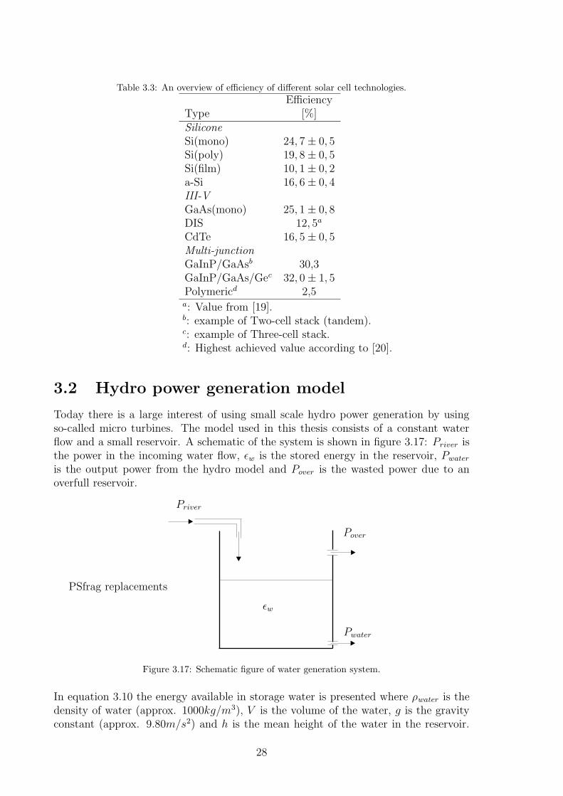
Table 3.3: An overview of efficiency of different solar cell technologies.

EfficiencyType [%]SiliconeSi(mono) 24, 7± 0, 5Si(poly) 19, 8± 0, 5Si(film) 10, 1± 0, 2a-Si 16, 6± 0, 4III-VGaAs(mono) 25, 1± 0, 8DIS 12, 5a

CdTe 16, 5± 0, 5Multi-junctionGaInP/GaAsb 30,3GaInP/GaAs/Gec 32, 0± 1, 5Polymericd 2,5a: Value from [19].b: example of Two-cell stack (tandem).c: example of Three-cell stack.d: Highest achieved value according to [20].

3.2 Hydro power generation model

Today there is a large interest of using small scale hydro power generation by usingso-called micro turbines. The model used in this thesis consists of a constant waterflow and a small reservoir. A schematic of the system is shown in figure 3.17: Priver isthe power in the incoming water flow, εw is the stored energy in the reservoir, Pwateris the output power from the hydro model and Pover is the wasted power due to anoverfull reservoir.

PSfrag replacements

Priver

εw

Pover

Pwater

Figure 3.17: Schematic figure of water generation system.

In equation 3.10 the energy available in storage water is presented where ρwater is thedensity of water (approx. 1000kg/m3), V is the volume of the water, g is the gravityconstant (approx. 9.80m/s2) and h is the mean height of the water in the reservoir.

28

The height of the reservoir was assumed to be 5m and that gives a mean height at2.5m.

Pwater =ρwaterV gh

3.6 · 106(3.10)

The complete system was assumed to have a efficiency of just 50 % to not overestimatethe influence of the water generation. In all other senses the hydro power model wasconsidered ideal.

3.3 Wind power generation model

In this section a model is proposed for generating simulated power output time se-ries from a wind turbine. The model is based on Markov models,“one-seventh powerlaw equation” [3] and data from a conventional wind turbine [22]. The model includesa possibility of adapting to different geographic areas with different yearly mean values.

In the area of wind power modelling many research years have been spent to makemodels and forecast for wind power generation. The methods vary quite a lot butall agree on statistical variations with some correlations between following factors andthe great importance of field measurement as basis of the simulation. The need fordescribing the wind power model statistically is discussed in [23]. It is well knownthat the wind speed distribution can be fitted to a Rayleigh distribution or the moregeneral Weibull distribution. This has been done in [23, 24, 25, 26] but differencesare in including the correlation between two consecutive values. Measurements areneeded to determine this correlations. These models are quite complicated and there-fore need large computational resources and that is not practical when the simulationis just a small part of the system simulation. Some of the models are adapted to windfarms [4, 25] and that adds more complexity to the problem. The wind direction hasa greater importance because of the shading effects of the other wind turbines in thefarm. Due to the greater complexity the model while be more extensive. For simulationof single wind turbines shading generally not included. In [27, 28] Markov models areused to simulate the values. A great advantage of using a Markov model is that it isnot distribution dependent and it is easy to use. In [27] Markov models are coupledto simulation of wind direction. A combination of simulating wind speed and winddirection is very useful because there is normally a strong correlation between speedand direction of the wind. In coastal areas (on land), where it could be beneficial toinstall wind turbines, there are normally great differences between land and sea wind.To determine the model factors, measurements of both wind speed and wind directionare needed. By using only one matrix the wind speed intervals must be large to stillhave a manageable number of elements. In [28] the authors have proposed two differentmodels, both based on the Markov theory. The first model is a Markov model with 19states. The transition probabilities were calculated using measured wind speed data.This method had only correlation between two consecutive values. In the second modelthe wind speed is divided into three regimes, weak (states 1-7), medium (states 4-12)and strong (states 11-19). Overlapping is allowed to enable single high/low values inone regime. A start regime is selected and the time for spending in each regime is

29

determined using the original measured data. The length of time in each regime isstochastic variable. On average the wind speed is 1/3 of time in the weak-wind regime,1/2 of time in medium-wind regime and 1/6 of time in the strong-wind regime. Thestep of the simulations is one hour. According to the authors a further split is neededin to three seasons, winter (120 days), midseason (77 days) and summer (168 days).In comparison with measured data the simulations methods had similar mean valuesand distributions.

3.3.1 Obtaining the measured data

As input for the model data were used that were obtained at Nasudden, Sweden.(57◦4’N18◦13’E) Nasudden is close the very south of Gotland. Nasudden is and has been fora long time used for studies of wind turbines. One of the world’s first 2 MW windturbines was installed in this location. More information regarding the wind turbinesat Nasudden can be found in [29].

Figure 3.18: Map of Gotland, Nasudden is marked.

The data used for determine the Markov models are measured at a height of ten metersand were of contentiously measured ten minutes mean values. The measurements wereconducted by the Department of Earth Sciences at the University of Uppsala 1992 until1994.

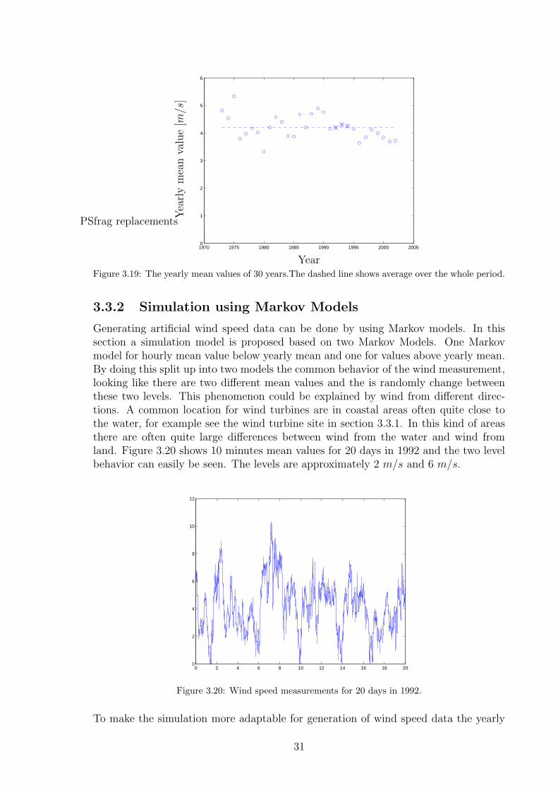
The mean values of the years from 1992 until 1994 were quite average years, as canbe seen in figure 3.19, where the yearly mean values are shown, 1992 until 1994 wereordinary years.

30

1970 1975 1980 1985 1990 1995 2000 20050

1

2

3

4

5

6

PSfrag replacements

Year

Yearlymeanvalue[m/s]

Figure 3.19: The yearly mean values of 30 years.The dashed line shows average over the whole period.

3.3.2 Simulation using Markov Models

Generating artificial wind speed data can be done by using Markov models. In thissection a simulation model is proposed based on two Markov Models. One Markovmodel for hourly mean value below yearly mean and one for values above yearly mean.By doing this split up into two models the common behavior of the wind measurement,looking like there are two different mean values and the is randomly change betweenthese two levels. This phenomenon could be explained by wind from different direc-tions. A common location for wind turbines are in coastal areas often quite close tothe water, for example see the wind turbine site in section 3.3.1. In this kind of areasthere are often quite large differences between wind from the water and wind fromland. Figure 3.20 shows 10 minutes mean values for 20 days in 1992 and the two levelbehavior can easily be seen. The levels are approximately 2 m/s and 6 m/s.

0 2 4 6 8 10 12 14 16 18 200

2

4

6

8

10

12

Figure 3.20: Wind speed measurements for 20 days in 1992.

To make the simulation more adaptable for generation of wind speed data the yearly

31

mean value was normalized to one. This can be done without change the distributionof wind speed which is together with the dependencies, for this case the interestinginformation. The Weibull distribution is most distribution fitted to wind data and thewind speed is in general considered according to this distribution [23, 24, 25, 26, 3].By normalizing the wind speed data the data could easily be adapted to any locationby scaling with the yearly mean wind speed value with the same distribution as theoriginal wind speed series.

By using measured wind speed data as input for the model it was possible to determinethe transition probability matrices for the Markov models. The two models were definedas if the last hourly mean value was above or below the yearly mean value. In the lowwind Markov model it is necessary to allow for some occasional high values becausehigh wind squalls exists. Low wind squalls also exist in the high wind so the high windmodel needs to take this in to account. The low wind model was discretized into 9levels while for the high wind model 14 levels were used. The higher number of levelsfor the high wind model is because large span of wind speeds. The mean value foreach level in the model was chosen so the yearly mean values of the simulated valueswould still be one. The intervals and mean, respectively for each level in the modelsare presented in table 3.4.

Table 3.4: The discretization of the wind speed data for the Markov models.

Low wind High windLevel Interval Mean value Interval Mean value

[m/s] [m/s] [m/s] [m/s]1 < 0.1 0.0325 < 0.7 0.57772 0.1-0.3 0.2230 0.7-0.9 0.84503 0.3-0.5 0.4090 0.9-1.1 1.02264 0.5-0.7 0.5989 1.1-1.3 1.20105 0.7-0.9 0.7984 1.3-1.5 1.39226 0.9-1.1 0.9772 1.5-1.7 1.58907 1.1-1.35 1.1708 1.7-1.9 1.78988 1.35-1.75 1.4651 1.9-2.1 1.99089 > 1.75 2.1356 2.1-2.3 2.191310 2.3-2.5 2.385911 2.5-2.7 2.586212 2.7-2.9 2.782513 2.9-3.25 3.030814 > 3.25 3.3892

The transition matrices can be estimated in many ways, the most intuitively is:

λij =fij

Σnk=1

fik(3.11)

where λij is the transition rate from state i to state j; fij is the number of transitionsfrom state i to state j in the input data set and n is the number of states in the each

32

of the models.

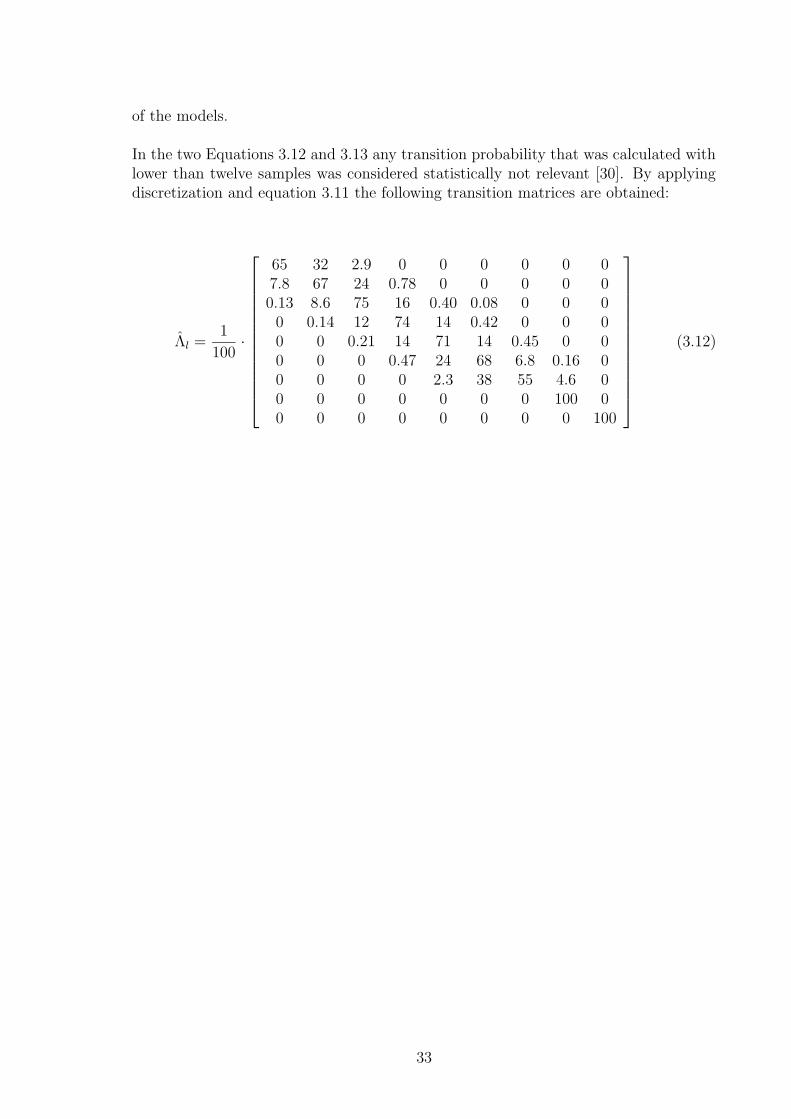
In the two Equations 3.12 and 3.13 any transition probability that was calculated withlower than twelve samples was considered statistically not relevant [30]. By applyingdiscretization and equation 3.11 the following transition matrices are obtained:

Λl =1

100·

65 32 2.9 0 0 0 0 0 07.8 67 24 0.78 0 0 0 0 00.13 8.6 75 16 0.40 0.08 0 0 00 0.14 12 74 14 0.42 0 0 00 0 0.21 14 71 14 0.45 0 00 0 0 0.47 24 68 6.8 0.16 00 0 0 0 2.3 38 55 4.6 00 0 0 0 0 0 0 100 00 0 0 0 0 0 0 0 100

(3.12)

33

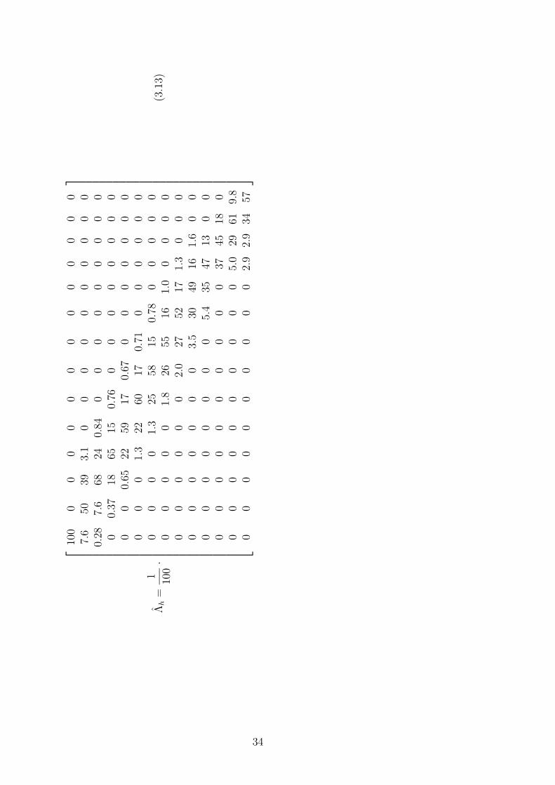
Λh=

1 100·

100

00

00

00

00

00

00

07.6

5039

3.1

00

00

00

00

00

0.28

7.6

6824

0.84

00

00

00

00

00

0.37

1865

150.76

00

00

00

00

00

0.65

2259

170.67

00

00

00

00

00

1.3

2260

170.71

00

00

00

00

00

1.3

2558

150.78

00

00

00

00

00

1.8

2655

161.0

00

00

00

00

00

2.0

2752

171.3

00

00

00

00

00

3.5

3049

161.6

00

00

00

00

00

5.4

3547

130

00

00

00

00

00

037

4518

00

00

00

00

00

05.0

2961

9.8

00

00

00

00

00

2.9

2.9

3457

(3.13)

34

Through use of equations 3.6-3.13 simulated wind speed data is obtained with a yearlymean value of one. This can be seen i figure 3.21 where the result of ten independentsimulations are shown. Each simulation had a length of 100 000 values and the meanvalue was 0.998. Each simulation started at mean value and in the low wind modelbut other simulations that started in the high wind model did not show any significantchange in the result. The transitions between the low and high models occurs whenthe mean value for the last hour passes 1.0.

1 2 3 4 5 6 7 8 9 100.99

0.995

1

1.005

1.01

1.015

Figure 3.21: Mean value of ten simulations.

Since the model is normalised according to the mean value location specifics could beincluded in the model by its yearly mean value. If the simulated wind speed data ismultiplied with the yearly mean value of the desired location artificial wind speed datacan be obtained. The data has the same distribution as the input data but with thelocal yearly mean value.

Figures 3.22 and 3.23 shows measured and simulated wind speed data series. Both theseries are normalized with mean value to one and are over a period of 2 months (8640values). In the figures the similarity is obvious.

The resemblance of Figures 3.22 and 3.23 are only statistically. The two differentlevels, earlier mentioned, can be seen in both but the latter one is more edged becauseof the discretization. The more edged appearance makes a small difference but it isunavoidable if the states should kept at a reasonable number.

3.3.3 Wind speed variations with height

The wind speed vary at different height and that is a well known fact. Measuring windspeed at many different heights are in most cases unpractical because you normally donot at what height you are interested in. By using an relationship between differentheights a measurement at a reference height is only needed. One common used rela-tionship is the power law also known as ”one-seventh power law equation” [3] and itcan also be known as Justus’ formula [31] and can be seen in equation 3.14.

35

0 10 20 30 40 50 600

0.5

1

1.5

2

2.5

3

3.5

Figure 3.22: Two months of measured wind speed data normalized to mean value of one.

0 10 20 30 40 50 600

0.5

1

1.5

2

2.5

3

3.5

Figure 3.23: Two months of simulated wind speed data normalized to mean value of one.

v(z2)

v(z1)=(z2

z1

)α

(3.14)

In equation 3.14, z1 is the height of the measurements and z2 is the height where thewind speed estimation is desired. v(z1) and v(z2) are wind speeds at height z1 andz2, respectively. α is the wind profile constant and is dependent on various factorse.g. height, wind speed, time of the day, season of the year, nature on the terrainand temperature. In [3] the authors have proposed a linear logarithm relationship,equation 3.15, to determined α and it is used in this model.

α = a− b · log10u(z1) (3.15)

Daytime are typical values or a and b 0.11 and 0.061 and for nighttime 0.38 and 0.209.Time considered as daytime are from 6.00 to 19.50 and the rest of the day is considered

36

nighttime. In Figure 3.15 is the relationship shown between the wind profile coefficientand wind speed.

5 10 15 20 25 30 35 40 45 50 55 600

0.05

0.1

0.15

0.2

0.25

0.3

0.35

0.4

Nighttime

Daytime

Figure 3.24: Wind profile coefficient α as a function of wind speed at z1.

3.3.4 Wind Turbine

There are many different ways of converting wind energy into electric energy. Thereare different types of wind turbines. The classical windmill has been used since theninth century. The windmills were used mainly in agriculture and another well-knownapplication of windmills was in draining the polders in The Netherlands whereas todaywind turbines are used to generate electricity for any purpose. This in large part due tothe possibility of transporting electrical energy over large distances and thus allowingany application. The wind turbines of today exists in a wide range of sizes, from lessthen 10 kW and up to offshore wind farms with tens of wind turbines of several MWeach.

The design of small wind turbine differs much from large turbines. Small turbinesare mostly direct-driven machines with variable speed and permanent magnets. Theaerodynamic profiles differs also and since manufacturers of wind turbine have a lessinterest in small turbines. The wing-profile of small turbines is less developed and theyare therefore less effective. A small turbines requires a higher rotor speed to be ableto achieve high reliability and low maintenance.

Large wind turbines were earlier designed according to the Danish Concept with fixedspeed, stall regulation and asynchronous generator. However this concept is more andmore replaced by newer technology. New concepts are based on variable speed withpitch control and either direct driven synchronous ring generator or doubly-fed asyn-chronous generator [32].

In this licentiate report a model is used to obtain the power output from a wind turbineusing the wind speed as input. This is achieved by using the so-called wind-power curveof a wind turbine. The wind-power curve is the relation between the wind speed andthe power output of the wind turbine and differs for different types of wind turbines.

37

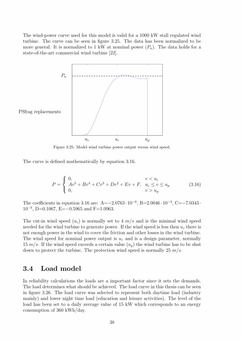
The wind-power curve used for this model is valid for a 1000 kW stall regulated windturbine. The curve can be seen in figure 3.25. The data has been normalized to bemore general. It is normalized to 1 kW at nominal power (Pn). The data holds for astate-of-the-art commercial wind turbine [22].

PSfrag replacements

uc ur up

Pn

Figure 3.25: Model wind turbine power output versus wind speed.

The curve is defined mathematically by equation 3.16.

P =

0, v < ucAv5 +Bv4 + Cv3 +Dv2 + Ev + F, uc ≤ v ≤ up0, v > up

(3.16)

The coefficients in equation 3.16 are: A=−2.0763 · 10−6, B=2.0046 · 10−4, C=−7.0343 ·10−3, D=0.1067, E=−0.5965 and F=1.0963.

The cut-in wind speed (uc) is normally set to 4 m/s and is the minimal wind speedneeded for the wind turbine to generate power. If the wind speed is less then uc there isnot enough power in the wind to cover the friction and other losses in the wind turbine.The wind speed for nominal power output is ur and is a design parameter, normally15 m/s. If the wind speed exceeds a certain value (up) the wind turbine has to be shutdown to protect the turbine. The protection wind speed is normally 25 m/s.

3.4 Load model

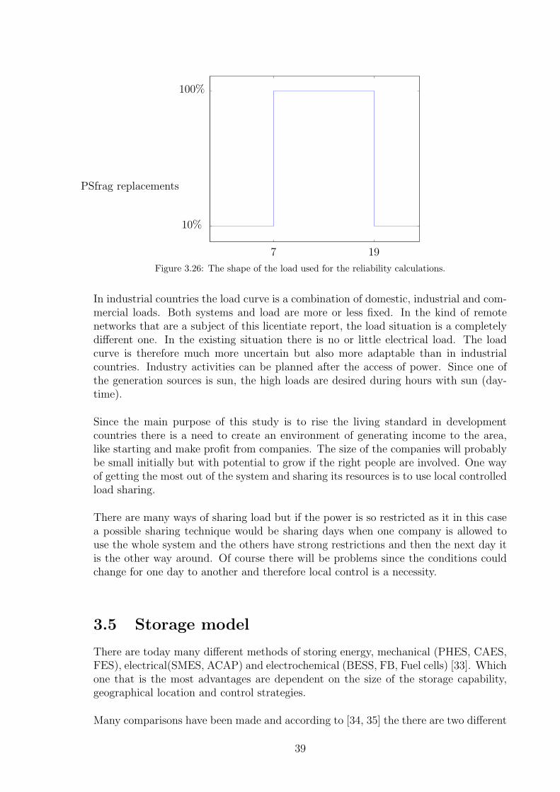
In reliability calculations the loads are a important factor since it sets the demands.The load determines what should be achieved. The load curve in this thesis can be seenin figure 3.26. The load curve was selected to represent both daytime load (industrymainly) and lower night time load (education and leisure activities). The level of theload has been set to a daily average value of 15 kW which corresponds to an energyconsumption of 360 kWh/day.

38

PSfrag replacements

7 19

10%

100%

Figure 3.26: The shape of the load used for the reliability calculations.

In industrial countries the load curve is a combination of domestic, industrial and com-mercial loads. Both systems and load are more or less fixed. In the kind of remotenetworks that are a subject of this licentiate report, the load situation is a completelydifferent one. In the existing situation there is no or little electrical load. The loadcurve is therefore much more uncertain but also more adaptable than in industrialcountries. Industry activities can be planned after the access of power. Since one ofthe generation sources is sun, the high loads are desired during hours with sun (day-time).

Since the main purpose of this study is to rise the living standard in developmentcountries there is a need to create an environment of generating income to the area,like starting and make profit from companies. The size of the companies will probablybe small initially but with potential to grow if the right people are involved. One wayof getting the most out of the system and sharing its resources is to use local controlledload sharing.

There are many ways of sharing load but if the power is so restricted as it in this casea possible sharing technique would be sharing days when one company is allowed touse the whole system and the others have strong restrictions and then the next day itis the other way around. Of course there will be problems since the conditions couldchange for one day to another and therefore local control is a necessity.

3.5 Storage model

There are today many different methods of storing energy, mechanical (PHES, CAES,FES), electrical(SMES, ACAP) and electrochemical (BESS, FB, Fuel cells) [33]. Whichone that is the most advantages are dependent on the size of the storage capability,geographical location and control strategies.

Many comparisons have been made and according to [34, 35] the there are two different

39

interesting cases of storage, load levelling (long term) and power quality (short term).The long term are often close connected to large storage while short term is stronglyconnected to a small storage capability which should only inject power if necessary.Methods of storage that are suitable for short term storage are BESS, SMES, ACAPand FES while for long term are BESS, CAES and PHES more suitable. Fuel cells orflow battery are also for long term storage since it require some startup time [34] andthe storage capability are almost only depend on the size of the storage tanks. Thestart time occurs because of the need of the chemical reaction to be reversed.

Here follows a short presentation of the today existing storage technologies.

Flow Batteries or regenerative fuels cells (FB)

In a storage system of flow batteries is energy stored as chemical potential energy. Thechemical potential energy will be created by ”charging” the two liquid electrolyte whenthey are pumped through a cell which has two electrodes and a proton exchange mem-brane when a potential is applied between the electrodes. The energy will be releasedwhen the procedure is reversed with a a load connected between the electrodes. Thereare many different couples of electrolytes and an example that is today commercial-ized is polysulphide/bromide and in equation 3.17 is the simplified overall chemicalreaction, for this combination of fuel cells, is shown.

3NaBr +Na2S4 ⇔ 2Na2S2 +NaBr3 (3.17)

The main advantage of flow batteries are that the are useful for utility-scale energystorage if combined with large storage of electrolyte. One of the disadvantages are thehazards of using and working with chemicals that are not environmental friendly [33].Today are the appears the focus be mainly in the automotive industry, like buses/truckswhich can be seen as isolated power system.

Super conducting Magnetic Energy Storage (SMES)

A super conducting magnetic energy storage is based on storage of energy in a mag-netic field of a super conducting coil. To obtain the super conducting state of the coilit must be held at cryogenic temperature. This requires a refrigerating system withuse of liquid helium or nitrogen [36, 37]. The super conducting coil can be config-ured as solenoid or a toroid. The solenoid is the most common due to its simplicityand cost effectiveness but the toroid-shape has been used in a number of small SMESsystems [36]. Energy can be stored for several month in a SMES system but it hasstill the access time is still just a few milliseconds. SMES has low maintenance due tono moving parts and its life time is independent of number of charges/discharges [37].Compared with other energy storage technologies SMES is still to costly be alternativebut previous studies have shown that micro (< 0.1 MWh) and midsize (1-100 MWh)has a great potential in the future on transmission and distribution levels. Use of hightemperature super conductors would also improve the cost effectiveness of the SMESin the future [36]. SMES has been used in a number of installations to mitigate powerquality disturbances [38].

40

Battery Energy Storage Systems (BESS)

Batteries are perhaps the most cost effective electrochemical energy storage. There aretoday many types of batteries, lead-acid, nickel-cadmium, hydride batteries, nickel-metal and lithium-ion etc., and the most used today is lead-acid [36] but nickel-cadmium is believed to be something for the future due to higher charge density andlower lifetime cost [34]. The lead-acid battery is today an mature technology and usedfor bulk energy storage and for rapid charge/discharge. A main disadvantages arethe low cycle life, low energy density and environmental hazard during the entire lifetime of the battery. The main advantages are low installation cost and possibilities forsealed battery, which is necessary for mobil applications [36]. The benefits from nickel-cadmium batteries are long life time, high reliability, low maintenance, low cycle costand environmental friendly [34]. Batteries are today a well used storage technology areare almost used everywhere.

Advanced Capacitors (ACAP)

An advanced capacitor stores energy in a electric field by accumulating a positive andnegative charges on two plates separated by an insulating dielectric. The energy E thatcan be stored in a capacitor can described by equation 3.18 where ε is the permittivityof the dielectric, A is the area of the plates, d is the distance between the plates andV is the voltage between the plates.

E =1

2

εA

d· V 2 (3.18)

Capacitors have today a limited use as large-scale energy storage device for power sys-tems and are today only used for short-term storage in power converters. In the futureceramic hyper capacitors and super capacitors (Ultra Capacitors) could be useable aslarge-scale storage in power systems. Ceramic hyper capacitors have a high withstandvoltage and a high dielectric strength but the are not good enough today to be useful.In cryogenic operation they appears to be more interesting but that is perhaps some-thing for the future. Super capacitors are double layers capacitors and thereby havean increase in storage capability. Super capacitors are most useful for high peak-load,low energy situations [36]. The number of charging/discharing cycles are above 106 fora ACAP and there is no decrease in storage capacity for increasing number of cycles[37]. ACAP is often used as very short-term storage in power converters and in smallmobile telecommunication devices (GSM) [36].

Flywheel Energy Storage (FES)

The methods of storing energy in Flywheel is based on the accelerating and retardationof a rotating mass. The energy stored in the flywheel can be described by equation 3.19where E is the energy, r is the radius of the mass, m is the weight of the mass, l is thelength of the mass and ω is the rotation velocity of the wheel.

E =r2mlω2

4(3.19)

41

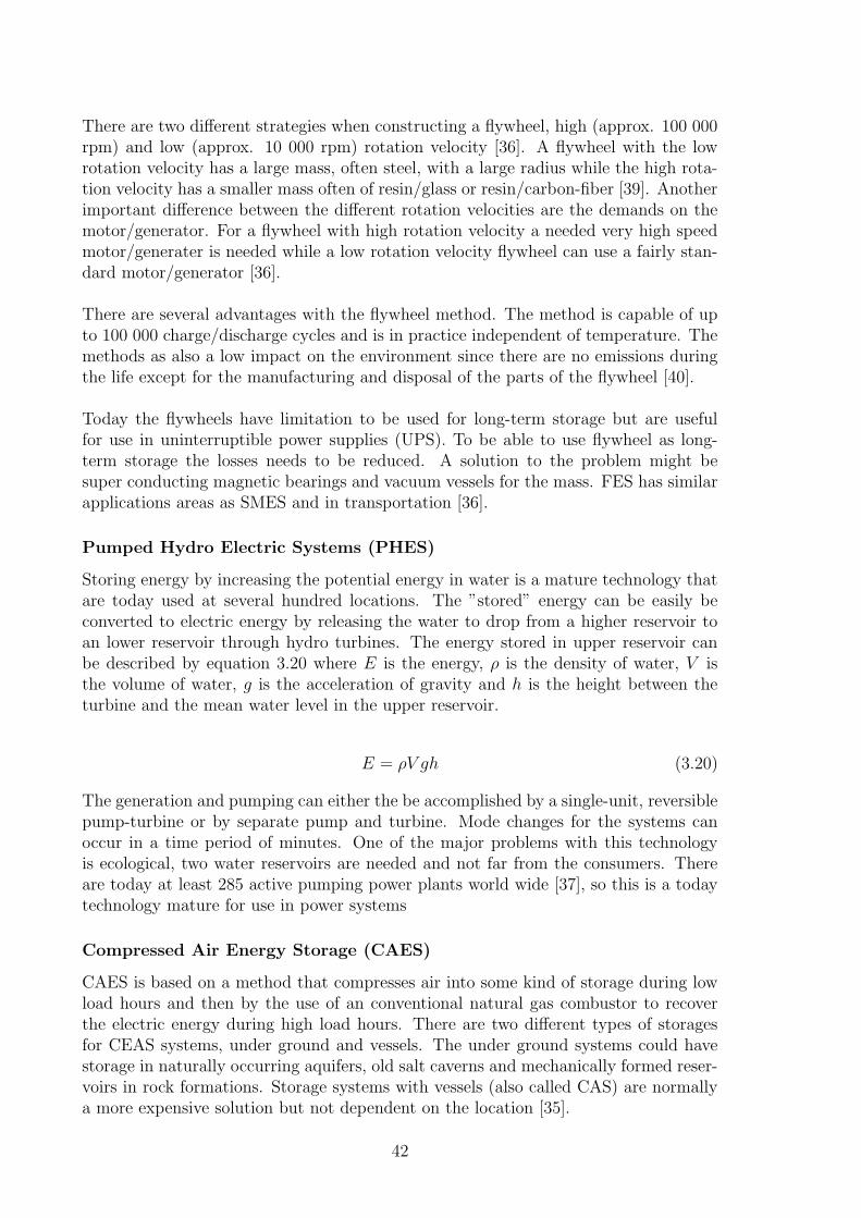
There are two different strategies when constructing a flywheel, high (approx. 100 000rpm) and low (approx. 10 000 rpm) rotation velocity [36]. A flywheel with the lowrotation velocity has a large mass, often steel, with a large radius while the high rota-tion velocity has a smaller mass often of resin/glass or resin/carbon-fiber [39]. Anotherimportant difference between the different rotation velocities are the demands on themotor/generator. For a flywheel with high rotation velocity a needed very high speedmotor/generater is needed while a low rotation velocity flywheel can use a fairly stan-dard motor/generator [36].

There are several advantages with the flywheel method. The method is capable of upto 100 000 charge/discharge cycles and is in practice independent of temperature. Themethods as also a low impact on the environment since there are no emissions duringthe life except for the manufacturing and disposal of the parts of the flywheel [40].

Today the flywheels have limitation to be used for long-term storage but are usefulfor use in uninterruptible power supplies (UPS). To be able to use flywheel as long-term storage the losses needs to be reduced. A solution to the problem might besuper conducting magnetic bearings and vacuum vessels for the mass. FES has similarapplications areas as SMES and in transportation [36].

Pumped Hydro Electric Systems (PHES)

Storing energy by increasing the potential energy in water is a mature technology thatare today used at several hundred locations. The ”stored” energy can be easily beconverted to electric energy by releasing the water to drop from a higher reservoir toan lower reservoir through hydro turbines. The energy stored in upper reservoir canbe described by equation 3.20 where E is the energy, ρ is the density of water, V isthe volume of water, g is the acceleration of gravity and h is the height between theturbine and the mean water level in the upper reservoir.

E = ρV gh (3.20)

The generation and pumping can either the be accomplished by a single-unit, reversiblepump-turbine or by separate pump and turbine. Mode changes for the systems canoccur in a time period of minutes. One of the major problems with this technologyis ecological, two water reservoirs are needed and not far from the consumers. Thereare today at least 285 active pumping power plants world wide [37], so this is a todaytechnology mature for use in power systems

Compressed Air Energy Storage (CAES)

CAES is based on a method that compresses air into some kind of storage during lowload hours and then by the use of an conventional natural gas combustor to recoverthe electric energy during high load hours. There are two different types of storagesfor CEAS systems, under ground and vessels. The under ground systems could havestorage in naturally occurring aquifers, old salt caverns and mechanically formed reser-voirs in rock formations. Storage systems with vessels (also called CAS) are normallya more expensive solution but not dependent on the location [35].

42

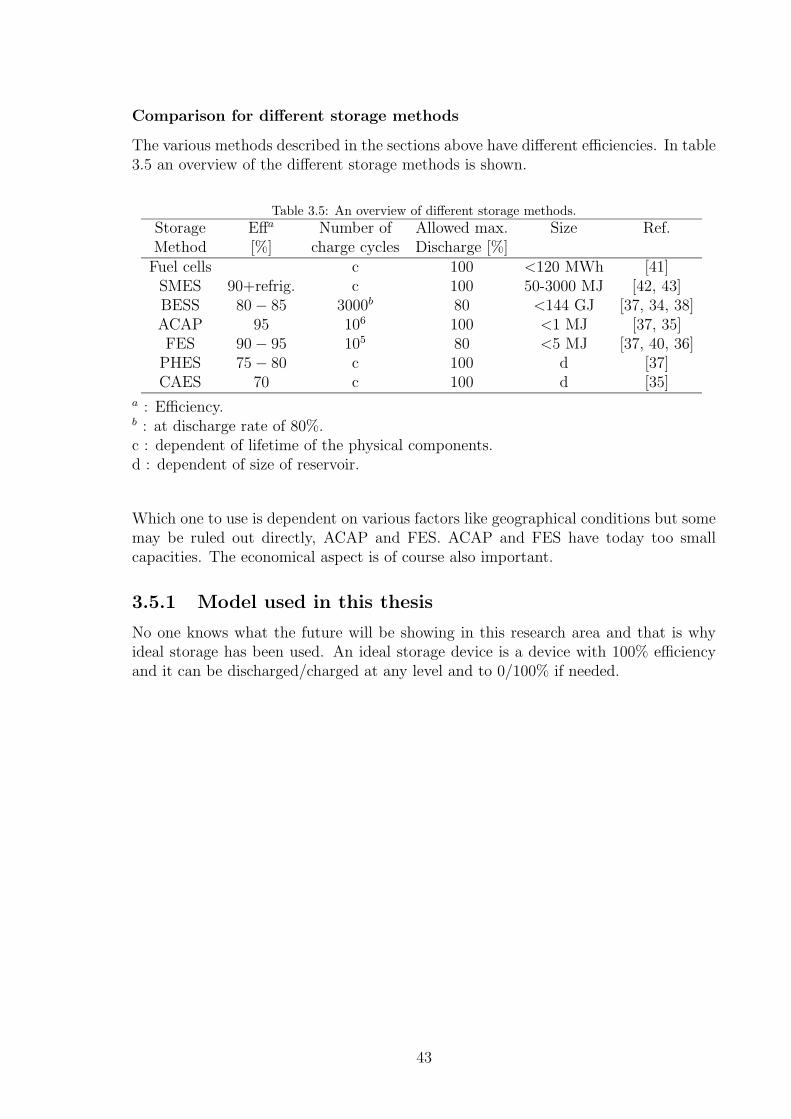
Comparison for different storage methods

The various methods described in the sections above have different efficiencies. In table3.5 an overview of the different storage methods is shown.

Table 3.5: An overview of different storage methods.

Storage Effa Number of Allowed max. Size Ref.Method [%] charge cycles Discharge [%]Fuel cells c 100 <120 MWh [41]SMES 90+refrig. c 100 50-3000 MJ [42, 43]BESS 80− 85 3000b 80 <144 GJ [37, 34, 38]ACAP 95 106 100 <1 MJ [37, 35]FES 90− 95 105 80 <5 MJ [37, 40, 36]PHES 75− 80 c 100 d [37]CAES 70 c 100 d [35]

a : Efficiency.b : at discharge rate of 80%.c : dependent of lifetime of the physical components.d : dependent of size of reservoir.

Which one to use is dependent on various factors like geographical conditions but somemay be ruled out directly, ACAP and FES. ACAP and FES have today too smallcapacities. The economical aspect is of course also important.

3.5.1 Model used in this thesis

No one knows what the future will be showing in this research area and that is whyideal storage has been used. An ideal storage device is a device with 100% efficiencyand it can be discharged/charged at any level and to 0/100% if needed.

43

Chapter 4

Case Study, Timbuktu

In this part of the thesis, the models presented in the previous chapter are used for anumber of case studies. All below listed combinations regarding the models are bothpresented individually and discussed. Twelve different cases were investigated:

• Solar power only

• Solar power with ideal storage

• Solar and hydro power

• Solar and hydro power with ideal storage

• Wind power only

• Wind power with ideal storage

• Solar and wind power

• Solar and wind power with ideal storage

• Wind and hydro power

• Wind and hydro power with ideal storage

• Solar, wind and hydro power

• Solar, wind and hydro power with ideal storage

Cases with only hydro or hydro with ideal storage are not considered. The hydro powermodel is constant and therefor gives no stochastic behavior.

45

In this chapter the following nomenclature is used:Psun Power generated by solar radiationPwind Power generated by windPwater Power generated by flow-of-river (hydro)Pload Load of the systemMGCsolar Maximum Generation Capacity for solar power generationMGCwind Maximum Generation Capacity for wind power generationεstor The energy in the ideal storageεstor(i) The energy in the ideal storage at current step in simulationεstor(i+ 1) The energy in the ideal storage at the following step in the simulationεmaxstor The maximum energy that could be stored in the ideal storage∆εstor The change of energy in the ideal storageεwater The energy in the reservoirεwater(i) The energy in the reservoir at current step in simulationεwater(i+ 1) The energy in the reservoir at the following step in the simulationεmaxwater The maximum energy that could be stored in the reservoir∆εwater The change of energy in the reservoir

The solar model requires a geographical location. For this study the location of Tim-buktu has been chosen, which is the capital of Mali in the southwest of Africa. Tim-buktu is located at a Latitude 16.75 ◦N and Longitude of 3.07 ◦W and the local timeis equal to the GMT. Timbuktu is chosen due to its location and the fact that Maliis a developming country with typical African/Sahara climate according to Koppen´sclimate classification system [15]. Figure 4.1 shows a map over Africa and Mali.

PSfrag replacements T imbuktu

Figure 4.1: A map over Africa showing Mali and Timbuktu.

Assumptions that has been made except those presented in the models are no lossesand no faults on the power system components. The control of the power system areassumed to be done by ideal power electronics. Meteorological data, used as input formodels, are due to lack of data from Timbuktu, measured in Sweden. Cloud coveragedata were collected at Save Airport, Goteborg and wind speed data were collected atNasudden, Gotland and at Save Airport, Goteborg.

46

To be able to relate the generation capacity used in the simulation to the load and tocompare different power sources the Maximum Generation Capacity (MGC) is used.The MGCsolar is the ratio between the theoretical maximum power generation (whenthe sun is in zenith during a cloudless day) and the maximum load for the solar powergeneration. MGCwind is calculated as the ratio between the rated wind power andmaximum load.

As described in Chapter 2 the basis of Monte-Carlo simulation are repeated simulations.In this case studies only one simulation is performed for each data point because asshown in Figure 4.2 little extra useful information will be achieved by repeating thesimulation. In the figure the solid line, showing the mean value of ten simulations, hasa very resemblance with the dashed line, that shows the result of only one simulation.By using only one simulation per data point computational time will be significantlyreduced.

0 1 2 3 4 5 6 7 8 9 100

0.05

0.1

0.15

0.2

0.25

0.3

0.35

0.4

PSfrag replacements

PsunPload

MGCsolar

Availab

ility

Figure 4.2: Availability of a power system with only solar power generation where the solid lineindicates the mean value of ten simulations while the dashed line is the result from a single simulation.

For the reliability calculations in this chapter a time step of one hour is used despite thestochastic varying models, presented in previous chapter, being developed for shortertime steps. From Figure 4.3 and 4.4 it can be concluded that the there is little needof smaller time steps then one hour in this kinds of calculations. Figure 4.3 showsthe the case of only solar power and load and Figure 4.4 shows a system where thepower generation originates from wind power. The differences seen in the figures arenot greater then the difference between two different simulations. A difference shouldnot occur because the mean value is independent on the length of the time steps. Insome cases the use of smaller time step is a necessity, like calculations of number oftimes shortage occurs and the duration of the shortages. This kinds of calculationsare anyway done in this thesis with a time step one hour. These studies are justan estimation of different system configurations and to be able to compare differentconfigurations and therefor shorter times are at this stage not necessary. Especiallywhen using storage or hydro, the short-term fluctuations in solar and wind will besmoothened out.

47

0 1 2 3 4 5 6 7 8 9 100

0.05

0.1

0.15

0.2

0.25

0.3

0.35

0.4

PSfrag replacements

MGCsolar

Availab

ility

Figure 4.3: A comparison between availability calculation with different time steps, one hour (solidline) and 6 minutes (dashed line).

0 1 2 3 4 5 6 7 8 9 100

0.1

0.2

0.3

0.4

0.5

0.6

0.7

PSfrag replacements

MGCwind

Availab

ility

Figure 4.4: A comparison between availability calculation with different time steps, one hour (solidline) and 10 minutes (dashed line).

4.1 Solar power only

The most simple power system and the first case in this study is a power systemwith only solar power as power source and no storage. In Figure 4.5 this system isschematically shown. The supplying energy and load are calculated according to earlierexplained models and the load is considered supplied if:

Psun ≥ Pload (4.1)

48

PSfrag replacements

Psun

Pload

Figure 4.5: Model of power flow in a small power system with only solar power as power source.

Figure 4.6 shows the availability as function ofMGCsolar. For large generation capacitythe availability nears 50 % but it never exceeds this level because the sun is above thehorizon for only 50% of the time. We also see that a large overcapacity is needed toobtain a reasonable availability. For a 40% availability (80% of day time), the installedcapacity should be about 10 times the maximum load. Figure 4.7 shows the loadand the power supply during a few days. It clearly indicates the lack of solar duringnighttime. But not only during night time does this lack of power exist. In dawnand in dusk there are also some problems because beginning and end of the powerproduction is dependent of the season since dawn and dusk change over the year andthe load, is assumed season-independent. The great 24 hours period dependence ismaybe the largest disadvantage of solar power generation. However, as we will seelater in combination with some other power sources solar power generation can beused.

0 1 2 3 4 5 6 7 8 9 10 11 12 13 14 15 16 17 18 19 200

0.05

0.1

0.15

0.2

0.25

0.3

0.35

0.4

0.45

PSfrag replacements

MGCsolar

Availab

ility

Figure 4.6: The availability of a system with only solar power.

49

60 61 62 63 64 65 66 67 68 69 70

0

2

4

6

8

10

12

14x 10

4

PSfrag replacements

Days

Pow

er[kW

]

Figure 4.7: A comparison between load (solid line) and available power (dashed line).

4.2 Solar power with ideal storage

By combining the solar power generation with storage the most obvious problems withsolar power can be avoided. As can be seen in Figure 4.7 the solar capacity oftenexceeds the load. But at other times the solar capacity is insufficient. By storing thedaytime surplus and use it at night, the availability will be improved. In Figure 4.8 amodel of the system is shown. The system uses solar power; the surplus of power isstored and then used when needed. The load is considered supplied if:

Psun + εstor(i) ≥ Pload (4.2)

The change in storage is calculated as follows:

∆εstor = Pload − Psun (4.3)

εstor(i+ 1) =

{

εstor(i) + ∆εstor ∆εstor < εstor(i)0 ∆εstor ≥ εstor(i)

(4.4)

unless εstor(i+ 1) exceeds εmaxstor then

εstor(i+ 1) = εmaxstor (4.5)

50

PSfrag replacements

Pwindεwater Storage

εstor

Psun

PwaterReservoir

Pload

Figure 4.8: Model of power flow in a small power system with use of solar power and ideal storage.

An important factor affecting the availability is the storage capacity (εmaxstor ) and thatis why Figure 4.9 shows the availability curve for five different storage capacities. Thenumber next to the lines represents the storage capacity, which is the number timesmaximum load. The line marked with 0 refers to a none-storage system as in Figure4.2. From this figure it can be concluded that 90% availability can be obtained with 7times maximum load of solar panels and 3 times maximum load of storage.

0 2 4 6 8 10 120

0.1

0.2

0.3

0.4

0.5

0.6

0.7

0.8

0.9

143

2

1

0

PSfrag replacements

MGCsolar

Availab

ility

Figure 4.9: A comparison between different maximum storage capacities. 0: none-storage system, 1:storage capacity equal to the maximum load, 2: Storage capacity twice the maximum load, 3: Storagecapacity of three times the maximum load and 4: storage capacity of four times the maximum load.

Figure 4.10 shows the energy level in the storage for a few days. A typical trend isnoticeable that the storage is filled during daytime and then emptied during nighttimewhich is expected for a solar power system. In the figure MGCsolar is 10.0 and themaximum storage is 3.0 times the maximum load.

51

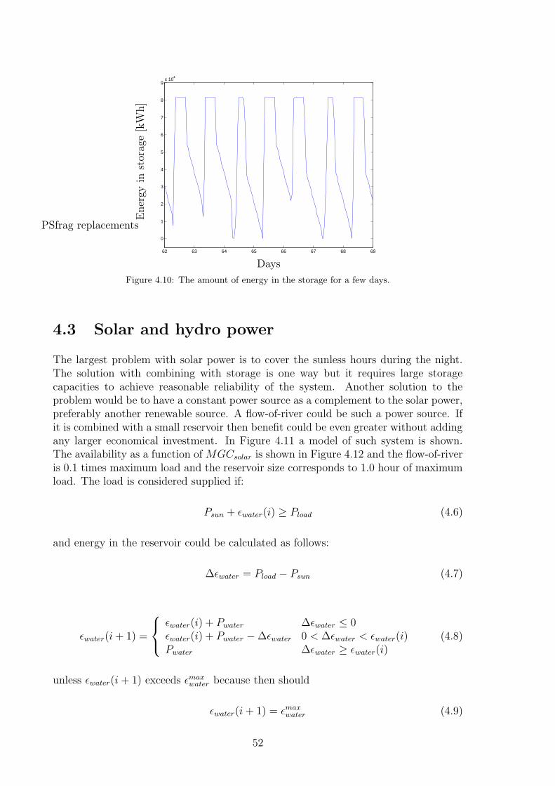
62 63 64 65 66 67 68 69

0

1

2

3

4

5

6

7

8

9x 10

4

PSfrag replacements

Days

Energy

instorag

e[kW

h]

Figure 4.10: The amount of energy in the storage for a few days.

4.3 Solar and hydro power

The largest problem with solar power is to cover the sunless hours during the night.The solution with combining with storage is one way but it requires large storagecapacities to achieve reasonable reliability of the system. Another solution to theproblem would be to have a constant power source as a complement to the solar power,preferably another renewable source. A flow-of-river could be such a power source. Ifit is combined with a small reservoir then benefit could be even greater without addingany larger economical investment. In Figure 4.11 a model of such system is shown.The availability as a function ofMGCsolar is shown in Figure 4.12 and the flow-of-riveris 0.1 times maximum load and the reservoir size corresponds to 1.0 hour of maximumload. The load is considered supplied if:

Psun + εwater(i) ≥ Pload (4.6)

and energy in the reservoir could be calculated as follows:

∆εwater = Pload − Psun (4.7)

εwater(i+ 1) =

εwater(i) + Pwater ∆εwater ≤ 0εwater(i) + Pwater −∆εwater 0 < ∆εwater < εwater(i)Pwater ∆εwater ≥ εwater(i)

(4.8)

unless εwater(i+ 1) exceeds εmaxwater because then should

εwater(i+ 1) = εmaxwater (4.9)

52

PSfrag replacements

Pwind

εwaterStorage

εstor

Psun Pwater

Reservoir

Pload

Figure 4.11: Model of power flow in a small power system with use of solar and hydro power.

0 2 4 6 8 10 12 140

0.1

0.2

0.3

0.4

0.5

0.6

0.7

0.8

0.9

143

2

0

PSfrag replacements

MGCsolar

Availab

ility

Figure 4.12: The availability of a system that combines solar energy, flow-of-river and a small reservoir.The numbers in the figure represents: 0: No part of hydro power used, 2: The power of hydrocorresponds to 7 % of maximum load, 3: The power of hydro corresponds to 10 % of maximum load,4: The power of hydro corresponds to 13 % of maximum load.

As seen in Figure 4.12 the difference of using a flow-of-river of 10 % instead of 7 %corresponding to maximum load is greater, due to the 10 % supplies the load to 100%during low load hours (night time). By increasing the hydro power part even further, isno use if the increase is not significantly so that the hydro power will be a significantlypart of maximum load.

The benefit of using a simple reservoir can be seen in Figure 4.13. The solid lineshows the availability as a function of capacity of the reservoir while the dashed lineshows the case without reservoir. The gain of using a reservoir is larger the greater thereservoir. The calculation without reservoir is of course independent of the reservoirsize. The fluctuation in the dashed curve are due to the random variations inherent tothe Monte-Carlo simulation.

53

0.5 1 1.5 2 2.5 30.5

0.55

0.6

0.65

0.7

0.75

0.8

0.85

0.9

0.95

1

PSfrag replacements

Reservoir Capacity [Maximum load]

Availab

ility

Figure 4.13: A comparison for power system with (solid) and without (dashed) reservoir.

4.4 Solar and hydro power with ideal storage

By adding the hydro power to the solar power generation the availability increasedsignificantly mainly during nighttime. By combining the system with storage capacitycould increase the availability of the system even further. A model of such a systemis shown in Figure 4.14 and the availability is calculated according to the equationsbelow. The load was considered supplied if:

Psun + εstor(i) + εwater(i) ≥ Pload (4.10)

and the energy in the storages will then be:

∆εstor = Pload − Psun (4.11)

∆εwater = Pload − Psun − εstor(i) (4.12)

εstor(i+ 1) =

{

εstor(i)−∆εstor ∆εstor < εstor(i)0 ∆εstor ≥ εstor(i)

(4.13)

εwater(i+ 1) =


(4.14)

if εstor and εwater exceed εmaxstor and εmaxwater, respectively then

εstor(i+ 1) = εmaxstor and εwater(i+ 1) = εmaxwater (4.15)

54

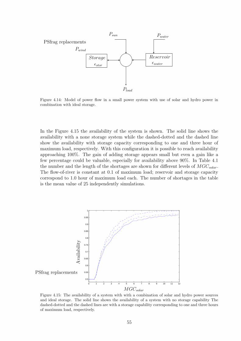
PSfrag replacements

Pwind

εwaterStorage

εstor

Psun Pwater

Reservoir

Pload

Figure 4.14: Model of power flow in a small power system with use of solar and hydro power incombination with ideal storage.

In the Figure 4.15 the availability of the system is shown. The solid line shows theavailability with a none storage system while the dashed-dotted and the dashed lineshow the availability with storage capacity corresponding to one and three hour ofmaximum load, respectively. With this configuration it is possible to reach availabilityapproaching 100%. The gain of adding storage appears small but even a gain like afew percentage could be valuable, especially for availability above 90%. In Table 4.1the number and the length of the shortages are shown for different levels of MGCsolar.The flow-of-river is constant at 0.1 of maximum load; reservoir and storage capacitycorrespond to 1.0 hour of maximum load each. The number of shortages in the tableis the mean value of 25 independently simulations.

0 1 2 3 4 5 6 7 8 9 10 11 12

0.5

0.55

0.6

0.65

0.7

0.75

0.8

0.85

0.9

0.95

1

PSfrag replacements

MGCsolar

Availab

ility

Figure 4.15: The availability of a system with with a combination of solar and hydro power sourcesand ideal storage. The solid line shows the availability of a system with no storage capability Thedashed-dotted and the dashed lines are with a storage capability corresponding to one and three hoursof maximum load, respectively.

55

Table 4.1: Number of shortages for different duration for different MGCsolar

MGCsolarDuration [h]1 2 5 10 20

1 10.8 114 176.6 154.3 120.22 0 145 80.2 53.83 29.4 8.3 58.14 84.4 80.4 39.75 57.2 22.7 9.66 25.8 16.87 6 1.68 0 09 0 010 0 011 0 012 265.9 96.6

Total shortages 474.9 567.9 364.1 208.1 120.2Total hours 4111.8 2135.2 718.1 261.9 120.2

Average h/short. 8.7 3.8 2.0 1.3 1.0

When the load is not supplied that just means that the load is not fully supplied.Figure 4.16 shows the power available for none-fully supplied hours with a MGCsolar

of 10.0. This power could still be used if some actions were taken to reduce the load.From this calculation it can be seen that for almost 10% of the none supplied hours theare less then 10% power is missing. Thus with a limited load reduction the availabilityof the rest of the load could be increased.

>90% 80−90% 70−80% 60−70% 50−60% 40−50% 30−40% 20−30% 10−20% <10%0

5

10

15

20

25

PSfrag replacements

Delivered Power

Number

ofShortages[%

]

Figure 4.16: The supplied power when the load was not supplied to 100%.

Another important aspect are the time of the day when the shortage occurs. In Figure4.17 the number of shortages are shown for each hour of the day. The power supplywas 5.0 MGCsolar and the power from flow-of-river corresponds to 0.1 times maximumload. The storage is 1.0 times maximum load for the storage as well as for the reservoir.

56

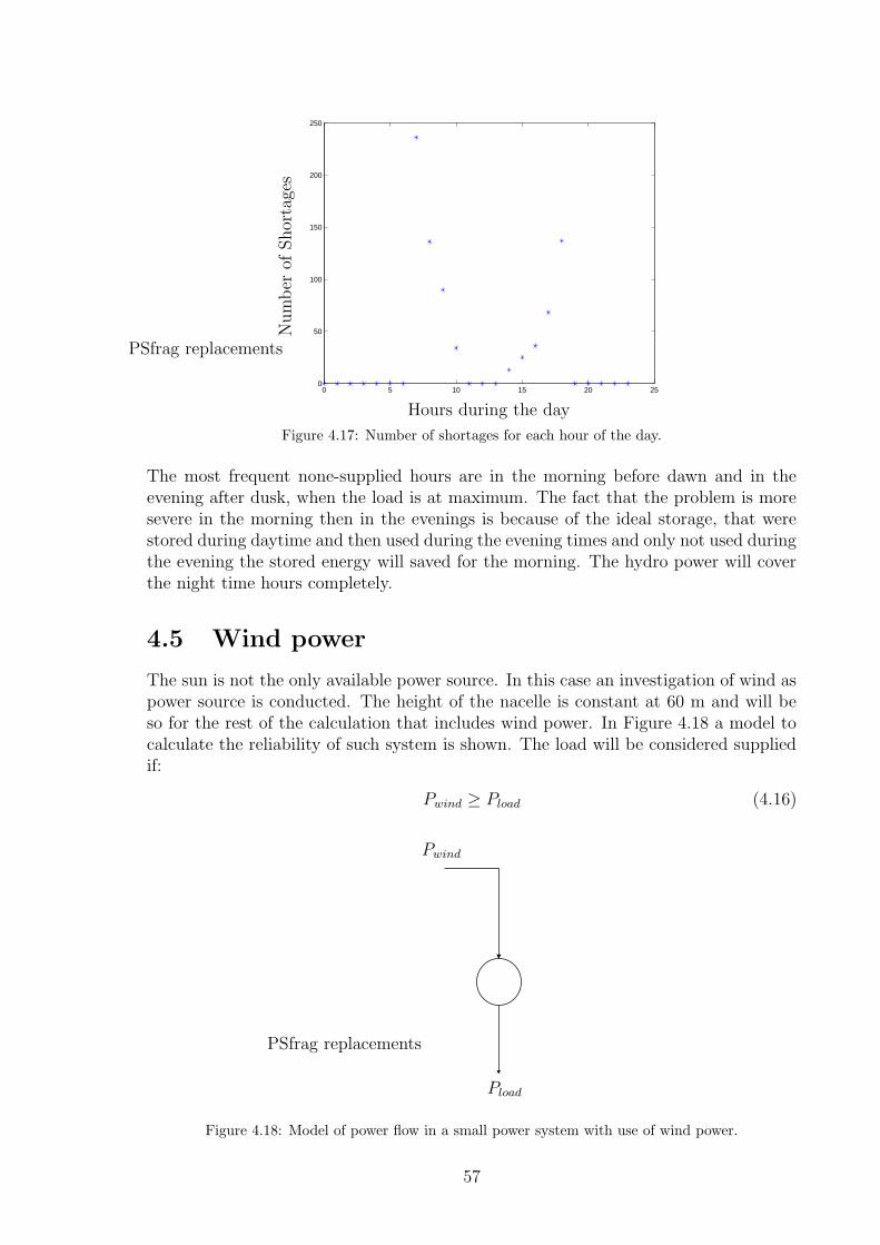
0 5 10 15 20 250

50

100

150

200

250

PSfrag replacements

Hours during the day

Number

ofShortages

Figure 4.17: Number of shortages for each hour of the day.

The most frequent none-supplied hours are in the morning before dawn and in theevening after dusk, when the load is at maximum. The fact that the problem is moresevere in the morning then in the evenings is because of the ideal storage, that werestored during daytime and then used during the evening times and only not used duringthe evening the stored energy will saved for the morning. The hydro power will coverthe night time hours completely.

4.5 Wind power

The sun is not the only available power source. In this case an investigation of wind aspower source is conducted. The height of the nacelle is constant at 60 m and will beso for the rest of the calculation that includes wind power. In Figure 4.18 a model tocalculate the reliability of such system is shown. The load will be considered suppliedif:

Pwind ≥ Pload (4.16)

PSfrag replacements

Pwind

Pload

Figure 4.18: Model of power flow in a small power system with use of wind power.

57

Figure 4.19 shows the availability for the system shown i Figure 4.18. Availability iscalculated for different values of MGCwind. Again a large overcapacity is needed toobtain an availability more than a few tens of percent. Availabilities more then 65%are hard to obtain with only wind power. Note that the fast fluctuations in Figure 4.19are ”stochastic noise” inherent to the Monte-Carlo simulation.

0 5 10 15 20 25 300

0.1

0.2

0.3

0.4

0.5

0.6

0.7

PSfrag replacements

MGCwind

Availab

ility

Figure 4.19: The availability of a system with only wind power.

The power supplied from wind power has not a regular (daily) pattern as solar powerhas. The fluctuations in wind power during a 10-day period can be seen in Figure 4.20.The availability differences between low and high load hours (i.e. between night andday) are small for wind power. The figure is calculated with MGCwind = 10.

60 61 62 63 64 65 66 67 68 69 700

0.5

1

1.5

2

2.5

3x 10

5

PSfrag replacements

Days

Pow

er[kW

]

Figure 4.20: A comparison between the power supplied by wind and the load.

4.6 Wind power with ideal storage

The irregularity of the wind power might be avoided by adding some storage capacity.A model of a wind power system with storage is shown in Figure 4.21. The availability

58

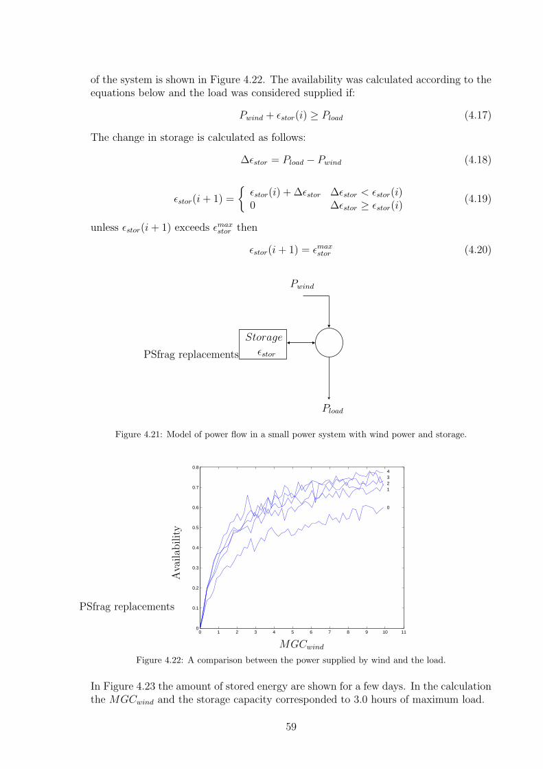
of the system is shown in Figure 4.22. The availability was calculated according to theequations below and the load was considered supplied if:

Pwind + εstor(i) ≥ Pload (4.17)

The change in storage is calculated as follows:

∆εstor = Pload − Pwind (4.18)

εstor(i+ 1) =

{


(4.19)



PSfrag replacements

Pwind

Pload

Storage

εstor

Figure 4.21: Model of power flow in a small power system with wind power and storage.

0 1 2 3 4 5 6 7 8 9 10 110

0.1

0.2

0.3

0.4

0.5

0.6

0.7

0.84321

0

PSfrag replacements

MGCwind

Availab

ility

Figure 4.22: A comparison between the power supplied by wind and the load.

In Figure 4.23 the amount of stored energy are shown for a few days. In the calculationthe MGCwind and the storage capacity corresponded to 3.0 hours of maximum load.

59

62 63 64 65 66 67 68 690

1

2

3

4

5

6

7

8

9x 10

4

PSfrag replacements

Days

Energy

instorag

e[kW

h]

Figure 4.23: The energy level in the storage for a few days.

4.7 Solar and wind power

By using solar and wind power the benefits from both power sources will be combined.A model of such system is shown in Figure 4.24. The availability can calculated asfollows. The load is considered supplied if:

Psun + Pwind ≥ Pload (4.21)

PSfrag replacements

Pwind

εwStorage

εstor

Psun

PwaterReservoir

Pload

Figure 4.24: Model of power flow in a small power system with use of solar and wind power.

The availability is shown in Figure 4.25 and for different amount of solar and windpower. The numbers in the figure are the value of MGCwind used for the calculation.The increase in availability due to the increase in the MGCwind decreases with highervalues ofMGCwind. This gives some kinds of limit for the useful amount of wind power.The exact value is probably dependent on the surrounding parameters.

60

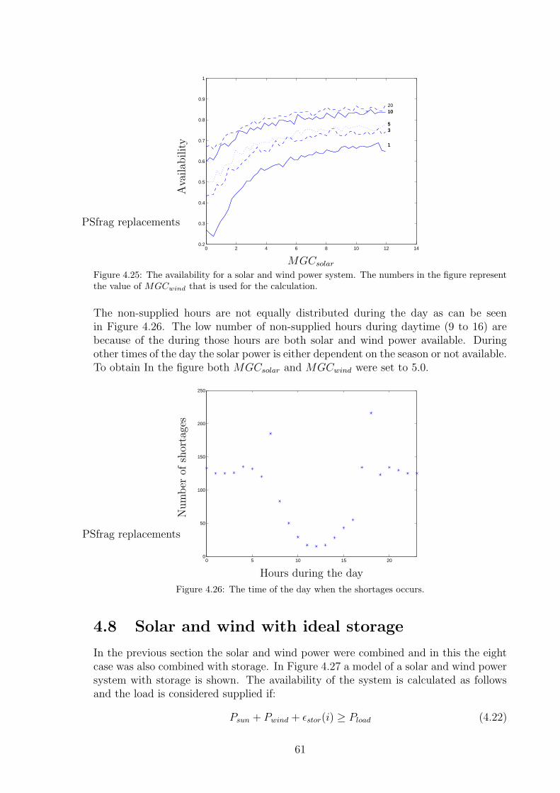
0 2 4 6 8 10 12 140.2

0.3

0.4

0.5

0.6

0.7

0.8

0.9

1

1

35

10

1

35

1020

PSfrag replacements

MGCsolar

Availab

ility

Figure 4.25: The availability for a solar and wind power system. The numbers in the figure representthe value of MGCwind that is used for the calculation.

The non-supplied hours are not equally distributed during the day as can be seenin Figure 4.26. The low number of non-supplied hours during daytime (9 to 16) arebecause of the during those hours are both solar and wind power available. Duringother times of the day the solar power is either dependent on the season or not available.To obtain In the figure both MGCsolar and MGCwind were set to 5.0.

0 5 10 15 200

50

100

150

200

250

PSfrag replacements


Number

ofshortages

Figure 4.26: The time of the day when the shortages occurs.

4.8 Solar and wind with ideal storage

In the previous section the solar and wind power were combined and in this the eightcase was also combined with storage. In Figure 4.27 a model of a solar and wind powersystem with storage is shown. The availability of the system is calculated as followsand the load is considered supplied if:

Psun + Pwind + εstor(i) ≥ Pload (4.22)

61

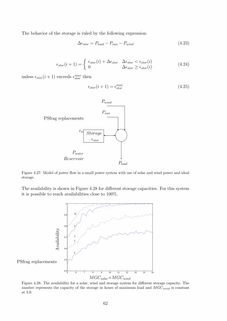
The behavior of the storage is ruled by the following expression:

∆εstor = Pload − Psun − Pwind (4.23)

εstor(i+ 1) =

{


(4.24)



PSfrag replacements

Pwind

εw Storage

εstor

Psun

PwaterReservoir

Pload

Figure 4.27: Model of power flow in a small power system with use of solar and wind power and idealstorage.

The availability is shown in Figure 4.28 for different storage capacities. For this systemit is possible to reach availabilities close to 100%.

5 6 7 8 9 10 11 12 13 14 150.4

0.5

0.6

0.7

0.8

0.9

1

10

5

3

1

0

PSfrag replacements

MGCsolar+MGCwind

Availab

ility

Figure 4.28: The availability for a solar, wind and storage system for different storage capacity. Thenumber represents the capacity of the storage in hours of maximum load and MGCwind is constantat 5.0.

62

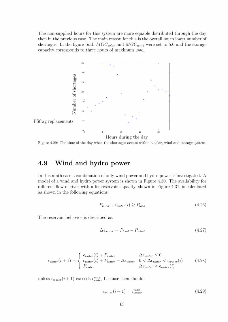
The non-supplied hours for this system are more equable distributed through the daythen in the previous case. The main reason for this is the overall much lower number ofshortages. In the figure both MGCsolar and MGCwind were set to 5.0 and the storagecapacity corresponds to three hours of maximum load.

0 5 10 15 200

5

10

15

20

25

30

35

PSfrag replacements


Number

ofshortages

Figure 4.29: The time of the day when the shortages occurs within a solar, wind and storage system.

4.9 Wind and hydro power

In this ninth case a combination of only wind power and hydro power is investigated. Amodel of a wind and hydro power system is shown in Figure 4.30. The availability fordifferent flow-of-river with a fix reservoir capacity, shown in Figure 4.31, is calculatedas shown in the following equations:

Pwind + εwater(i) ≥ Pload (4.26)

The reservoir behavior is described as:

∆εwater = Pload − Pwind (4.27)

εwater(i+ 1) =


(4.28)

unless εwater(i+ 1) exceeds εmaxwater because then should:


63

PSfrag replacements

Pwind

εwStorage

εstorPsun

Pwater

Reservoir

Pload

Figure 4.30: Model of power flow in a small power system with use of wind and hydro power.

0 1 2 3 4 5 6 7 8 9 10 11 12 13 14 150

0.1

0.2

0.3

0.4

0.5

0.6

0.7

0.8

0.9

0

1

23

PSfrag replacements

MGCwind

Availab

ility

Figure 4.31: The availability of a wind and hydro power systems for different values of available hydropower. 0: No Flow-of-river, 1: The flow-of-river corresponds to 5% of maximum load, 2: The flow-of-river corresponds to 10% of maximum load, 3: The flow-of-river corresponds to 20% of maximumload.

Figure 4.31 shows among others the effect of flow-of-river. The benefit of increasingflow-of-river is small after the 10% limit is reached, because the 10% is enough to supplythe system during low load hours (nighttime). The increase in availability for increaseflow-of-river above 10% is almost not noticeable, because of the power generation ofthe flow-of-river is small compared to maximum load. When the flow-of-river increasesmuch more to be a significant part of maximum load, then that will of course make ahuge difference in the availability.

4.10 Wind and hydro power with ideal storage

In the previous case the wind and hydro system was investigated. An improvementof the system would be to add storage capacity to the system, a model shown in

64

Figure 4.32. The availability of wind and hydro system with storage, seen in Figure4.33, is calculated as in the following equations. The load is considered supplied if:

Pwind + εstor(i) + εwater(i) ≥ Pload (4.30)

The behavior of the storage and reservoir is obtained from:

∆εstor = Pload − Pwind (4.31)

∆εwater = Pload − Pwind − εstor(i) (4.32)

εstor(i+ 1) =

{


(4.33)

εwater(i+ 1) =


(4.34)

If εstor and εwater exceed εmaxstor and εmaxwater, respectively then


PSfrag replacements

Pwind

εwaterStorage

εstor

Psun

Pwater

Reservoir

Pload

Figure 4.32: Model of power flow in a small power system with use of wind and hydro power systemwith storage capacity.

65

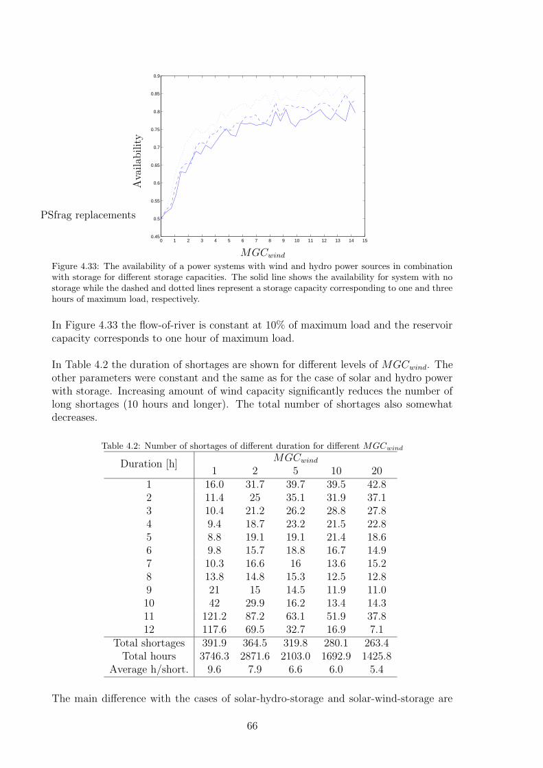
0 1 2 3 4 5 6 7 8 9 10 11 12 13 14 150.45

0.5

0.55

0.6

0.65

0.7

0.75

0.8

0.85

0.9

PSfrag replacements

MGCwind

Availab

ility

Figure 4.33: The availability of a power systems with wind and hydro power sources in combinationwith storage for different storage capacities. The solid line shows the availability for system with nostorage while the dashed and dotted lines represent a storage capacity corresponding to one and threehours of maximum load, respectively.

In Figure 4.33 the flow-of-river is constant at 10% of maximum load and the reservoircapacity corresponds to one hour of maximum load.

In Table 4.2 the duration of shortages are shown for different levels of MGCwind. Theother parameters were constant and the same as for the case of solar and hydro powerwith storage. Increasing amount of wind capacity significantly reduces the number oflong shortages (10 hours and longer). The total number of shortages also somewhatdecreases.

Table 4.2: Number of shortages of different duration for different MGCwind

MGCwindDuration [h]1 2 5 10 20

1 16.0 31.7 39.7 39.5 42.82 11.4 25 35.1 31.9 37.13 10.4 21.2 26.2 28.8 27.84 9.4 18.7 23.2 21.5 22.85 8.8 19.1 19.1 21.4 18.66 9.8 15.7 18.8 16.7 14.97 10.3 16.6 16 13.6 15.28 13.8 14.8 15.3 12.5 12.89 21 15 14.5 11.9 11.010 42 29.9 16.2 13.4 14.311 121.2 87.2 63.1 51.9 37.812 117.6 69.5 32.7 16.9 7.1


Average h/short. 9.6 7.9 6.6 6.0 5.4

The main difference with the cases of solar-hydro-storage and solar-wind-storage are

66

for high values of MGC. In the solar-hydro-storage case the power source is more reg-ular then in the solar-wind-storage case and that effects mainly the high MGC-valueswhere the solar case has no shortages with a duration longer than 5.0 hours.

In Figure 4.34 the MGCwind was 5.0 and the flow-of-river corresponded to 10% of themaximum load and the reservoir and storage capacity were corresponding to 1.0 hourof maximum load each. The main delivered power when the load is not supplied isbetween 10 and 20 % which is the contribution of the hydro power without wind andstorage at daytime load.

>90% 80−90% 70−80% 60−70% 50−60% 40−50% 30−40% 20−30% 10−20% <10%0

10

20

30

40

50

60

PSfrag replacements

Delivered Power

Number

ofShortages[%

]

Figure 4.34: The generation capacity during the hours when the load was not fully supplied.

When the non-supplied hours occurs during the day. In Figure 4.35 the number ofhours that is non-supplied shown for each hour of the day. The low number of short-ages during night time is when the hydro power supplies the load completely. Duringdaytime the hydro only supplies 10% of the load and then is the non-regular behaviorof wind. During the morning hours the shortages are fewer than during the rest of theday because of the storage. In the figure MGCwind = 5, storage capacity correspondsto one hour of maximum load and flow-of-river is 0.1 times the maximum load.

67

0 5 10 15 200

50

100

150

200

250

PSfrag replacements


Number

ofshortages

Figure 4.35: The hours of the day when the load was not fully supplied.

4.11 Solar, wind and hydro power

Another investigated case is a system, a model shown in Figure 4.36, with a combinationof solar, wind and hydro power. The availability of such a system is shown in Figure4.37, for different flow-of-river, and was calculated according to the equations below.The load was considered supplied if:

Psun + Pwind + εwater(i) ≥ Pload (4.36)

The behavior of the water level in the reservoir was calculated from:

∆εwater = Pload − (Psun + Pwind) (4.37)

εwater(i+ 1) =


(4.38)

unless εwater(i+ 1) exceeds εmaxwater because then should


68

PSfrag replacements

Pwind

εwStorage

εstor

Psun Pwater

Reservoir

Pload

Figure 4.36: Model of power flow in a small power system with use of solar, wind and hydro power.

The Figure 4.37 the MGCwind is constant and the MGCsolar varies. Here can also beeseen that the hydro limit of 0.1 time the maximum load (dotted and highest solid lines)is important to obtain high reliability.

5 6 7 8 9 10 11 12 13 140.4

0.5

0.6

0.7

0.8

0.9

1

0

1

23

PSfrag replacements

MGCsolar+MGCwind

Availab

ility

Figure 4.37: The availability of a power systems with solar, wind and hydro power sources for differentflow-of-river. The solid line marked 0 the availability for system with no flow-of-river (no hydro) whilethe lines marked 1, 2 and 3 represents systems with flow-of-river that corresponds to 5%, 10% and20% of maximum load, respectively.

Table 4.3 shows the duration of the shortages in the system with MGCwind was setto 5.0 and the flow-of river corresponded to 10% of maximum load. The values ofnumber of shortages in the table are the mean values of 25 independent simulations.The number of shortages decreases significantly with increasing MGCsolar because ofthe regularity of the solar power. The same behavior can be seen in Figure 4.1. Thevalues are lower because of the power supplied from wind power.

69

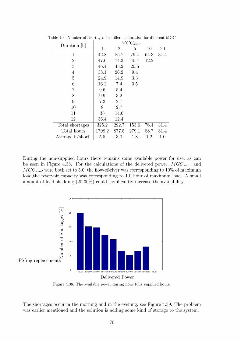
Table 4.3: Number of shortages for different duration for different MGC


1 42.8 85.7 79.4 64.3 31.42 47.6 74.3 40.4 12.23 46.4 43.2 20.64 38.1 26.2 9.45 24.9 14.9 3.36 16.2 7.4 0.57 9.6 5.48 9.9 3.29 7.3 2.710 8 2.711 38 14.612 36.4 12.4


Average h/short. 5.5 3.0 1.8 1.2 1.0

During the non-supplied hours there remains some available power for use, as canbe seen in Figure 4.38. For the calculations of the delivered power, MGCsolar andMGCwind were both set to 5.0, the flow-of-river was corresponding to 10% of maximumload,the reservoir capacity was corresponding to 1.0 hour of maximum load. A smallamount of load shedding (20-30%) could significantly increase the availability.

>90% 80−90% 70−80% 60−70% 50−60% 40−50% 30−40% 20−30% 10−20% <10%0

5

10

15

20

25

PSfrag replacements

Delivered Power

Number

ofShortages[%

]

Figure 4.38: The available power during none fully supplied hours.

The shortages occur in the morning and in the evening, see Figure 4.39. The problemwas earlier mentioned and the solution is adding some kind of storage to the system.

70

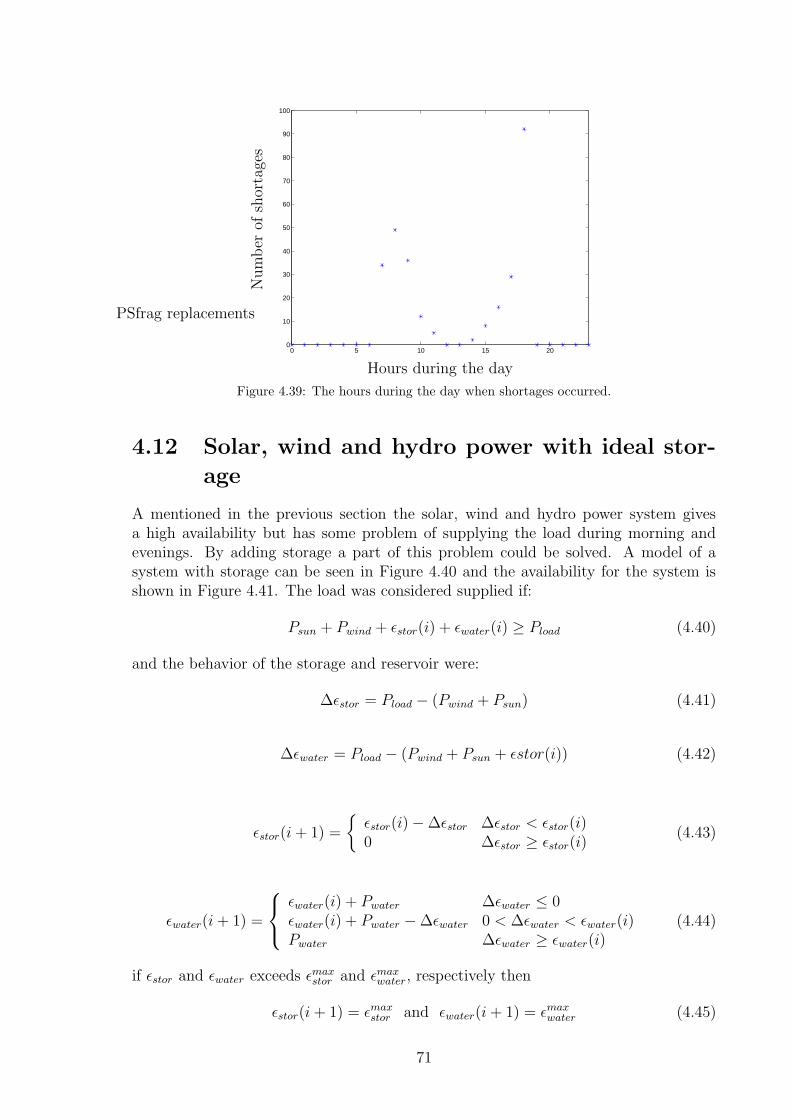
0 5 10 15 200

10

20

30

40

50

60

70

80

90

100

PSfrag replacements


Number

ofshortages

Figure 4.39: The hours during the day when shortages occurred.

4.12 Solar, wind and hydro power with ideal stor-

age

A mentioned in the previous section the solar, wind and hydro power system givesa high availability but has some problem of supplying the load during morning andevenings. By adding storage a part of this problem could be solved. A model of asystem with storage can be seen in Figure 4.40 and the availability for the system isshown in Figure 4.41. The load was considered supplied if:

Psun + Pwind + εstor(i) + εwater(i) ≥ Pload (4.40)

and the behavior of the storage and reservoir were:

∆εstor = Pload − (Pwind + Psun) (4.41)

∆εwater = Pload − (Pwind + Psun + εstor(i)) (4.42)

εstor(i+ 1) =

{


(4.43)

εwater(i+ 1) =


(4.44)

if εstor and εwater exceeds εmaxstor and εmaxwater, respectively then


71

PSfrag replacements

Pwind

εwStorage

εstor

Psun Pwater

Reservoir

Pload

Figure 4.40: Model of power flow in a small power system with use of different renewable energysources.

6 8 10 12 14 160.7

0.75

0.8

0.85

0.9

0.95

1

0

1

3

PSfrag replacements

MGCsolar+MGCwind

Availab

ility

Figure 4.41: The availability for a system with solar, wind, hydro and different capacities of thestorage. The numbers represents the capacities of the storage, corresponding to maximum load.MGCwind was 5.0 for the calculation.

Durations of the shortages are shown in Table 4.4 and the differences between thenumber of shortages are increasing compared to the previous case 4.3 with increasinggeneration. That is because of the greater importance of the storage since more energyis produced and thereby is availably for storage and thereby later use. The values ofnumber of shortages in the table are the mean values of 25 independent simulations.

72

Table 4.4: Number of shortages for different duration for different MGC


1 57.1 78.5 51.7 30.5 10.72 51.8 53.4 29.0 6.23 45.0 34.2 14.94 36.1 18.8 6.25 23.6 11.0 1.46 15.4 7.57 8.2 4.68 7.1 2.69 6.6 2.410 8.0 3.111 33.3 11.312 18.7 6.8

Total shortage 310.9 234.2 103.2 36.7 10.7Total hours 1494.8 774.6 186.2 42.9 10.7

Average h/short. 4.8 3.3 1.8 1.2 1.0

Power available during none-fully supplied hours of system with solar, wind and hydropower with storage are shown in Figure 4.42. The MGCsolar and MGCwind were set to5.0 and the flow-of-river corresponds to 10% of maximum load. The storage and thereservoir capacities corresponded to 1.0 hour of maximum load.

>90% 80−90% 70−80% 60−70% 50−60% 40−50% 30−40% 20−30% 10−20% <10%0

2

4

6

8

10

12

14

16

18

PSfrag replacements

Delivered Power

Number

ofShortages[%

]

Figure 4.42: The available power for non-fully supplied hours.

In Figure 4.43 the times during the day when the shortages occur is shown. Thebehavior of the number of shortages is similar to the one in the case of solar, wind andhydro power without storage, see Figure 4.39, but the absolute numbers are lower. Inthis case can be seen that a load shedding of 30% will half the unavailability.

73

0 5 10 15 200

5

10

15

20

25

30

35

40

45

50

PSfrag replacements


Number

ofshortages

Figure 4.43: The available power for none-fully supplied hours.

4.13 Discussions of Case studies

One of the greatest differences between solar and wind power are the regularity ofthe solar power. This is both the advantage and the disadvantage of the solar power.Which one to use is dependent on the surrounding source, equipment and demand ofcourse.

In the case of only one power source and no storage the one most available source iswind but the picture is a little more complicated. The overall availability is better forthe wind power but that is only when the average is taken for the whole year. Thesolar power system has a significantly higher availability during daytime, see Table 4.5.Since the wind power only has a small difference between day and night time the largedifference in the availability are due to the great difference in load between day andnight time.

Table 4.5: Availability for night and day for solar and wind power

Night daySolar power 0 0.61Wind power 0.64 0.41

The same thing can be seen in Figure 4.44 where the high availability for solar duringday time is shown by low number of shortages during daytime. For night time almost allthe 4380 hours are not supplied. The wind power system has a more even distributionduring the 24 hours period. The differences between day and night are due to earliermentioned differences in the load.

74

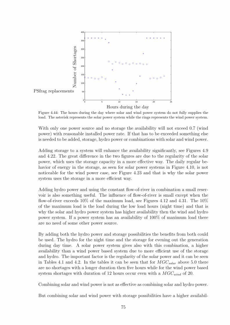
0 5 10 15 20 250

50

100

150

200

250

300

350

400

PSfrag replacements


Number

ofShortages

Figure 4.44: The hours during the day where solar and wind power system do not fully supplies theload. The asterisk represents the solar power system while the rings represents the wind power system.

With only one power source and no storage the availability will not exceed 0.7 (windpower) with reasonable installed power rate. If that has to be exceeded something elseis needed to be added, storage, hydro power or combinations with solar and wind power.

Adding storage to a system will enhance the availability significantly, see Figures 4.9and 4.22. The great difference in the two figures are due to the regularity of the solarpower, which uses the storage capacity in a more effective way. The daily regular be-havior of energy in the storage, as seen for solar power systems in Figure 4.10, is notnoticeable for the wind power case, see Figure 4.23 and that is why the solar powersystem uses the storage in a more efficient way.

Adding hydro power and using the constant flow-of-river in combination a small reser-voir is also something useful. The influence of flow-of-river is small except when theflow-of-river exceeds 10% of the maximum load, see Figures 4.12 and 4.31. The 10%of the maximum load is the load during the low load hours (night time) and that iswhy the solar and hydro power system has higher availability then the wind and hydropower system. If a power system has an availability of 100% of maximum load thereare no need of some other power source.

By adding both the hydro power and storage possibilities the benefits from both couldbe used. The hydro for the night time and the storage for evening out the generationduring day time. A solar power system gives also with this combination, a higheravailability than a wind power based system due to more efficient use of the storageand hydro. The important factor is the regularity of the solar power and it can be seenin Tables 4.1 and 4.2. In the tables it can be seen that for MGCsolar above 5.0 thereare no shortages with a longer duration then five hours while for the wind power basedsystem shortages with duration of 12 hours occur even with a MGCwind of 20.

Combining solar and wind power is not as effective as combining solar and hydro power.

But combining solar and wind power with storage possibilities have a higher availabil-

75

ity the solar and hydro power and the same as the solar and hydro power with storage.As can be seen in Figures 4.17 and 4.29 the case of solar and wind power based systemhas a more even distribution of the shortages during the day than the solar and hydrobased system. A more even distribution is to prefer because the consequences of ashortage during day time (high load) will be worse then during night time (low load).

Combining solar, wind and hydro power and storage will be as expected even morebeneficial for the availability. The shortages will occur during morning and eveningsdue to the lack of solar radiation.

In this discussion so far only fully supplied hours have been discussed. During a short-age the available power is not zero and the power could be used if the load is adaptedto the situation. The available power during none-fully supplied hours is shown in thischapter for selected cases.

In this chapter the cases has all been discussed in an availability point of view but inalmost every case the economical aspect is at least as important. But that aspect isnot covered in this thesis.

76

Chapter 5

Conclusions

Two stochastic models are proposed in this thesis. A solar model based on cloud cover-age is one of the models. A way to simulate cloud coverage data with reduced need formeteorological data is also presented. The second model is for simulating wind speed.It also reduces the need for meteorological measurements. Both the models are basedon Markov theory.

A system with only one power source, only wind power has a higher availability thansolar power but solar power has a more regular behavior. All power produced by solaris produced during daytime which will give higher availability during day-time thanwind power.

Combining a single power source (wind or solar) with storage, the availability increasessignificantly. Solar power gives a higher availability because the regularity and therebythe more efficient use of the storage.

Adding a small hydro source in combination with wind or solar power will increase theavailability further because it will supply the load during low load hours.

Combining solar and wind power gives a high reliability during daytime when bothsolar and wind power are available. The problem is during night-time when only windis available. Adding hydropower covers the lowload period that occurs during night-time. The main problems occur when the high day-time load begins before the solarpower is available at sufficient extent and at dusk when the load is still at day-time level.

To be able to use exclusively renewable energy sources a combination of sources isneeded to secure the reliability of the supply. It is also important to adjust the loadlevels to the availability of the renewable sources.

77

Chapter 6

Future Work

This thesis is just a small part of the research area addressed. The area of isolatedpower systems based entirely on renewable energy is just in its cradle. There are manyaspects that are not investigated in this thesis and that is something for future work.

Probably most important are the economical aspects for this kind of systems. It isimportant to keep the focus on supplying activities that could generate income to thearea, like products that can be sold outside of the area.

In the case studies and in the models all components have been assumed ideal and thenon-ideal behavior is something to include. This would require more detailed knowl-edge of the components used.

One of the larger problems of introducing new technologies is the social acceptance,especially when the level of technology is low before the introduction. The reliabilityand robustness of the system required for social acceptance also need to be furtherinvestigated.

The models presented in this thesis are independent. Future development of the modelswould be to introduce dependencies between wind, sun and the supply of hydro power.That dependencies exists is obvious for a extreme dry year the supply of hydro will bebad but the solar power will then be larger. More generally, each of these sources willshow a seasonal variation.

In this thesis the load model is deterministic and that is just a rough estimation of thea real load. The load model should also be stochastic and even dependent on meteoro-logical conditions. The stochastic element becomes more important in a small system.Some loads are weather-dependent which introduces additional dependencies. Furtherinvestigations should include load-shedding policies when low generation capacity isexpected.

The power system use in this thesis has been modelled as a single node. By introduc-ing a realistic power system some other aspects would need to be studied like thermaloverload during warm weather.

How should this systems be controlled? What kind of power electronics equipment is

79

needed? That are other important questions that have to be answered before use ofisolated power systems with only renewable energy sources.

80

References

[1] R. Billinton and R. Allan, Reliability Evaluation of Power Systems. Plenum Press,1996.

[2] B. Lindgren, Power-generation, Power-electronics and Power-systems issues ofpower Converters for photovoltaic applications. Chalmers University of Technol-ogy, 2002.

[3] L. Johnson, Wind Energy Systems. Prentice-Hall, Inc., 1985.

[4] P. Sørensen, A. Hansen, and P. Rosas, “Wind models for simulation of powerfluctuations from wind farms,” Journal of Wind Engineering and Industrial En-gineering, vol. 90, no. 12, pp. 1381–1402, 2002.

[5] A. Høyland and M. Rausand, System Reliability Theory - Models and StatisticalMethods. John Wiley & Sons, Inc., 1994.

[6] R. Gallager, Discrete Stochastic Processes. Kluwer Academic Publishers, 1996.

[7] S. Ross, Introduction to Probability Models. Academic Press, Inc., 1989.

[8] R. Billinton and W. Li, Reliability Assessment of Electric Power Systems UsingMonte Carlo Methods. Plenum Press, 1994.

[9] G. Fishman, Monte Carlo - Concepts, Algorithms and Applications. Springer,1996.

[10] U. Amato, A. Andretta, B. Bartoli, B. Coluzzi, V. Cuomo, F. Fontana, and C. Se-rio, “Markov processes and fourier analysis as a tool to describe and simulate dailysolar irradiance,” Solar energy, vol. 37, no. 3, pp. 179–194, 1986.

[11] D. Albizzatia, G. Rossetti, and O. Alfano, “Measurements and predictions ofsolar radiation incident on horizontal surfaces at Santa Fe, Argentina (31◦ 39’S,60◦ 43’W),” Renewable Energy, vol. 11, no. 4, pp. 469–478, 1997.

[12] A. Balouktsis and P. Tsalides, “On stochastic simulation of hourly total solar radi-ation sequences,” International Journal of Energy Systems, vol. 8, no. 3, pp. 1121–125, 1988.

[13] V. Graham and K. Hollands, “A method to generate synthetic hourly solar ra-diaition globally,” International Journal of Solar Energy, vol. 44, no. 6, p. 333,1990.

81

[14] A. Balouktsis and P. Tsalides, “Stochastic simulation model of hourly total solarradiation,” International Journal of Solar Energy, vol. 37, no. 2, p. 119, 1986.

[15] R. Stull, Meteorology Today For Scientists and Engineers: A Technical CompanionBook. West Publishing Company, 1995.

[16] L. Nielsen, L. Prahm, R. Berkowicz, and K. Conradsen, “Net incoming radiationestimated from hourly global radiation and/or cloud observations,” Journal ofClimatology, vol. 1, no. 3, p. 255, 1981.

[17] P. Jones, “Cloud-cover distribution and coorrelations,” Journal of Applied mete-orolgy, vol. 31, p. 732, 1992.

[18] U. Hjort, Computer Intensive Statistical Methods: Validation, Model Selection andBootstrap. Chapman & Hall, 1995.

[19] G. Boyle, Renewable Energy - power for a sustainable future. Oxford UniversityPress, 1996.

[20] M. Svensson, F. Zhang, S. Veenstra, W. Verhees, J. Hummelen, J. Kroon, O. In-ganas, and M. Andersson, “High-performance polymer solar cells of an alternatingpolyfluorene copolymer and a fullerene derivative,” Advanced Materials, vol. 15,no. 12, pp. 988–991, 2003.

[21] M. Green, K. Emery, D. King, S. Igari, and W. Warta, “Solar cells efficiency tables(version 22),” Progress in Photovoltics: Reasearch and Applications, vol. 11, no. 5,pp. 347–352, 2003.

[22] http://www.nwp.se, “Tekniska data: Nordic 1000.”

[23] R. Billinton and L. Gan, “Wind power modeling and application in generatingadequacy assessment,” in IEEE WESCANEX 93. Communications, Computersand Power in the Modern Environment Conference Proceedings, (Saskatoon, Sask.,Canada), pp. 100–106, May 17-18, 1993.

[24] S. Biswas, B. Sraedhar, and Y. Singh, “A simplified statistical technique for windturbine energy output estimation.,” Wind Engineering, vol. 19, no. 3, pp. 147–155,1995.

[25] A. Feijoo, J. Cidras, and J. Dornelas, “Wind speed simulation in wind farms forsteady-state security assessment of electrical power systems,” IEEE transactionson Energy Conversion, vol. 14, no. 4, pp. 1582–1588, 1999.

[26] L. Kamal and Y. Jafri, “Time series models to simulate and forecast hourly av-eraged wind speed in Quetta, Pakistan.,” Solar Energy, vol. 61, no. 1, pp. 23–32,1997.

[27] P. Sparis, J. Antonogiannakis, and D. Papadopoulos, “Markov matrix coupledapproach to wind speed and direction simulation,” Wind Engineering, vol. 19,no. 3, pp. 121–133, 1999.

82

[28] C. Masters, J. Mutale, G. Strbac, S. Curcic, and N. Jenkins, “Statistical evalu-ation of voltages in distribution systems with embedded wind generation.,” IEEProceedings-Generation, Transmission and Distribution, vol. 147, no. 4, pp. 217–212, 2000.

[29] G. Ronsten, S.-E. Thor, H. Ganander, H. Johansson, T. Thiringer, T. Petru, andH. Bergstrom, “Evaluation of loads, power quality, grid interaction, meteorolog-ical condition and power performance of this first swedish offshore wind farm atBockstigen,” in (OWEMES ´00), (Syracuse, Italy), April 13-14, 2000.

[30] Gold Book; Recommended Practice for the Design of Reliable Industrial and Com-mercial Power Systems. IEEE Inc., 1998.

[31] G. Notton, M. Muselli, P. Poggi, and A. Louche, “Decentralized wind energysystems providing small electric loads in remote areas.,” International journal ofenergy research, vol. 25, pp. 141–164, 2001.

[32] T. Ackermann and L. Soder, “An overview of wind energy-status 2002,” Renewableand Sustainable Energy Reviews, vol. 6, no. 1-2, pp. 67–128, 2002.

[33] A. Price and B. Davidson, “Recent developments in the design and applicationsof utility-scale energy storage plant,” in Electricity Distribution, 2001. Part 1:Contributions. CIRED. 16th International Conference and Exhibition on, (Ams-terdam, Netherlands), p. 4.22, 18-21 June, 2001.

[34] J. McDowall, “Nickel-cadmium batteries for energy storage applications,” in Bat-tery Conference on Applications and Advances, 1999. The Fourteenth Annual,(Long Beach,CA,USA), pp. 303–308, 1999.

[35] S. Schoenung and C. Burns, “Utility energy storage applications studies,” IEEEtransactions on Energy Conversion, vol. 11, no. 3, pp. 658–665, 1996.

[36] P. Ribeiro, B. Johnson, M. Crow, A. Arsoy, and Y. Liu, “Energy storage sys-tems for advanced power applications,” Proceedings of the IEEE, vol. 89, no. 12,pp. 1744–1756, 2001.

[37] T. Sels, C. Dragu, T. Van Craenenbroeck, and R. Belmans, “Overview of new en-ergy storage systems for an improved power quality and load managing of distribu-tion level.,” in Electricity Distribution, 2001. Part 1: Contributions. CIRED. 16thInternational Conference and Exhibition on, (Amsterdam, Netherlands), p. 4.26,18-21 June, 2001.

[38] M. Bollen, Understanding power quality problems: voltage sags and interruptions.IEEE Press, 2000.

[39] J. Boyes and N. Clark, “Technologies for energy storage. flywheels and super con-ducting magnetic energy storage.,” in Power Engineering Society Summer Meet-ing, 2000. IEEE, (Seattle, WA, USA), pp. 1548–1550, 2000.

[40] L. Reinke and P. Eng, “Tutorial overview of flywheel energy storage in a photo-voltaic power generation system,” in Electrical and Computer Engineering, 1993.Canadian Conference on, (Vancouver, BC, Canada), pp. 1161–1164, 1993.

83

[41] I. Grant, “Tva’s regenesys energy storage project,” in Power Engineering SocietySummer Meeting, 2002 IEEE, (Tennessee Valley Authority, Chattanooga, TN,USA), pp. 321–322, 2002.

[42] V. Karasik, K. Dixson, B. Weber, G. Campbell, and P. Ribeiro, “SMES for powerutility applications: A review of technical and cost considerations,” IEEE trans-actions on applied superconductivity, vol. 9, no. 2, pp. 541–546, 1999.

[43] C. Loungo, “Superconducting storage systems: An overview,” IEEE Transactionson Magnetics, vol. 32, no. 4, pp. 2214–2223, 1996.

84

generation reliability for isolated power sys- tems with...

Documents