generative adversarial networks for reconstructing natural ...€¦ · generative adversarial...

Generative adversarial networks for reconstructingnatural images from brain activity

K. Seeliger∗, U. Guclu, L. Ambrogioni, Y. Gucluturk, M. A. J. van Gerven

Radboud UniversityDonders Institute for Brain, Cognition and Behaviour

Montessorilaan 3, 6525 HR Nijmegen, The Netherlands

December 8, 2017

KeywordsVision, reconstruction, generative adversarial networks, fMRI

Abstract

We explore a straightforward method for reconstructing visual stimuli from brain activity.Using large databases of natural images we trained a deep convolutional generative adversar-ial network capable of generating gray scale photos, similar to stimuli presented during twofunctional magnetic resonance imaging experiments. Using a linear model we learned to pre-dict the generative model’s latent random vector z from measured brain activity. The objectivewas to create an image similar to the presented stimulus image through the previously trainedgenerator. Using this approach we were able to reconstruct natural images, but not to an equalextent for all images with the same model. A behavioral test showed that subjects were ca-pable of identifying a reconstruction of the original stimulus in 67.6% and 64.4% of the casesin a pairwise test for the two natural image datasets respectively. Our approach does not re-quire end-to-end training of a large generative model on limited neuroimaging data. As theparticular GAN model can be replaced with a more powerful variant, the current advances ingenerative modeling promise further improvements in reconstruction performance.

1 Introduction

Since the advent of functional magnetic resonance imaging (fMRI), numerous new research di-rections that leverage its exceptional spatial resolution, leading to classifiable brain activity pat-terns, have been explored (Haynes, 2015). New approaches to decoding specific brain states havedemonstrated the benefits of pattern-based fMRI analysis. Pattern-based decoding from the vi-sual system has shown that it is possible to decode edge orientation (Kamitani and Tong, 2005),perceived categories of both static and dynamic stimuli (Haxby, 2001; Huth et al., 2016), up toidentifying a specific stimulus image (Kay et al., 2008) and generically identifying new categoriesfrom image descriptors predicted from brain activity (Horikawa and Kamitani, 2017).

Here we focus on an advanced problem in brain decoding, which is actually reconstructinga perceived (natural) visual stimulus. The reconstruction problem is demanding since the set ofpossible stimuli is effectively infinite. This problem has been explored at different spatial scales(e.g. invasively on the cellular level (Chang and Tsao, 2017)) and in different regions of the visualsystem (e.g. in the LGN (Stanley et al., 1999), in the retina (Parthasarathy et al., 2017)). Here wefocus on image reconstruction from brain activity measured with fMRI. This area was pioneeredby Thirion et al. (2006), who reconstructed dot patterns with rotating Gabors from perceptionand imagery. Miyawaki et al. (2008) used binary 10 × 10 images as stimuli and demonstrated

∗Corresponding author: B [email protected]

1

not certified by peer review) is the author/funder. All rights reserved. No reuse allowed without permission. The copyright holder for this preprint (which wasthis version posted December 8, 2017. . https://doi.org/10.1101/226688doi: bioRxiv preprint

https://doi.org/10.1101/226688

the possibility of decoding pixels independently from each other, reconstructing arbitrary newimages with this basis set. Naselaris et al. (2009) introduced a combination of encoding brainactivity with structural and semantic features, as well as a Bayesian framework to identify themost likely stimulus image from a very large image database given the brain activity. Combiningthe most likely stimuli from a database leads to effective reconstructions, with (Nishimoto et al.,2011) being the most impressive example to date. Bayesian approaches were further developed.Examples are enhancing decoding using feature sets learned with independent component anal-ysis (Guclu and van Gerven, 2013) and accurate reconstruction of handwritten characters usingstimulus domain priors and a linear model for predicting brain activity (Schoenmakers et al.,2013, 2015). The most recent entries in the reconstruction domain make use of promising newdevelopments in generative image models. Du et al. (2017) used Bayesian inference to derivemissing latent variables, and effectively reconstruct handwritten digits and 10 × 10 binary im-ages. Finally, adversarial training has been used for reconstructing face photos from fMRI withhigh detail by learning to encode to and decode from a learned latent space for faces (Gucluturket al., 2017).

In this work we expand on the generative model idea, but explore the capabilities of a methodthat applies a natural image generative model as a black box which is trained without using(usually limited) neuroimaging data. We pretrain a deep convolutional generative adversarialnetwork (DCGAN) (Radford et al., 2015), capable of producing arbitrary images from the stim-ulus domain (handwritten characters or natural gray scale images). Keeping this GAN fixed welearn to predict the latent space of the generator z based on the fMRI BOLD signal in response toa presented stimulus. The objective is achieving high similarity between the generated and theoriginal image in the image domain. The image domain losses that are used to train the predic-tive model are derived with a complex loss function. We show that this approach is capable ofgenerating reasonable reconstructions from fMRI data for the given stimulus domains.

2 Methods

2.1 Functional MRI data sets

We made use of three publicly available fMRI data sets originally acquired for experiments re-lated to identifying stimulus images and categories or reconstruction of perception. In the fol-lowing we briefly list their properties. Extensive descriptions of recording details and methodscan be found in the original publications.

2.1.1 Handwritten characters

We used this dataset (referred to as BRAINS dataset) to test our method in a simpler, restricteddomain. Three subjects were presented with gray scale images of 360 examples of six handwrittencharacters (B, R, A, I, N and S; as published with Van der Maaten (2009); Schomaker and Vuurpijl(2000)) with fixation in a 3T fMRI experiment (TR=1.74 s, voxel size=2 mm3). The images wereshown for 1 s at 9 × 9◦ of visual angle, flashed at approximately 3 Hz. The characters wererepeated twice, and responses were averaged. The original studies reconstructed handwrittencharacters using a linear decoding approach (Schoenmakers et al., 2013) and Gaussian mixturemodels (Schoenmakers et al., 2015). We made use of the preprocessed data from V1 and V2available in the BRAINS dataset and used the original train / test set split (290 and 70 charactersrespectively). The dataset can be downloaded from www.artcogsys.com.

2.1.2 Masked natural images

Three subjects saw natural gray scale images with a circular mask, taken from different sources(the commercial Corel Stock Photo Libraries from Corel Corporation, and the Berkeley Segmen-tation Dataset) at 20 × 20◦ of the visual field with fixation. The dataset and experiments were

2


https://doi.org/10.1101/226688

described in (Kay et al., 2008) and (Naselaris et al., 2009). The training set consisted of 1750 im-ages, presented twice and averaged. The test set consisted of 120 images, presented 13 times.Images were presented for 1 s and flashed at approximately 3 Hz. Data was acquired in a 4Tscanner (TR=1 s, voxel size=2 × 2 × 2.5 mm3). The dataset is available on www.crcns.orgunder the identifier vim-11, which is also how we refer to it in this manuscript. We obtaineda version of the dataset with updated preprocessing for all three subjects from the author viapersonal communication. In our study we used the first 50 images from the original validationdataset as a test set, and the remainder of the data for training. The advantage of the dataset forthis study is the amount of data and the variety of high-quality photo stimuli.

2.1.3 Natural object photos

This dataset was originally recorded for (Horikawa and Kamitani, 2017), and is referred to asGeneric Object Decoding dataset. Five subjects were presented with square colour imagesfrom 150 categories from the ImageNet database (Deng et al., 2009). We converted the stimulusimages to gray scale and applied a similar mild contrast enhancement as in (Kay et al., 2008) in-stead of using the full color stimuli for reconstruction2. We also used the original train / test setsplit. The training set consisted of 8 images from each category and was presented once, totaling1200 presentations. The test set recording consisted of presenting single images of 50 categories(not contained in the training set) 35 times each, and averaging this activity. The data can beobtained from www.brainliner.jp3. Next to having recordings of five subjects one advantageof this dataset is the long stimulation time of 9 s (at 2 Hz flashing) per image, resulting in a highsignal-to-noise ratio (SNR). All images were presented at 12 × 12◦ of visual angle, with fixation,in a 3T scanner (TR=3 s, voxel size= 3 mm3).

The data of the individual subjects of all datasets were mapped to a common representationalspace based on hyperalignment (Haxby et al., 2011) using PyMVPA4 (Hanke et al., 2009). Hy-peraligned data was averaged across subjects such as to obtain data for a single hyperalignedsubject with improved SNR5. After hyperalignment, the dimensionality of the feature (voxel ac-tivity) space was reduced by applying principal component analysis (PCA, including demean-ing) so that 99% (BRAINS, Generic Object Decoding) or 90% (vim-1, due to its much largervoxel dimension) were preserved. Hyperalignment, PCA and statistical parameters (e.g. meanvalues) were computed on the training sets and applied on the training and the separate test set.For these additional preprocessing steps we used the single trial data for vim-1 and GenericObject Decoding, as the different averaging strategies changed SNR between train and test.For BRAINS we used the provided data averages over two trials as there was no such differencebetween the train and test recordings.

2.2 Generative Adversarial Networks

Generative Adversarial Networks (GANs) learn to synthesize elements of a target distributionpdata (e.g. images of natural scenes) by letting two neural networks compete. Their results tendto have photo-realistic qualities. The Generator network (G) takes an n-dimensional randomsample from a predefined distribution – conventionally called latent space z – and attempts tocreate an example G(z) from the target distribution, with z as initial values. In the case of imagesand deep convolutional GANs (DCGANs), introduced in (Radford et al., 2015), this is realized

1https://crcns.org/data-sets/vc/vim-1 (last access May 2017)2We focus on reconstructing gray scale images as our natural images DCGAN learned to generate more structural

detail when the color dimension was omitted. However with a more powerful GAN variant the method could also beapplied for reconstructing color stimuli.

3http://brainliner.jp/data/brainliner/Generic Object Decoding (last access August 2017)4www.pymvpa.com, v2.6.35Our method was initially developed on the individual subject basis. This only seemed to lead to more variability in

the reconstruction quality between subjects, and we decided to finalize the study on hyperaligned data instead as thismade collecting behavioral data and developing the loss function more efficient.

3


https://doi.org/10.1101/226688

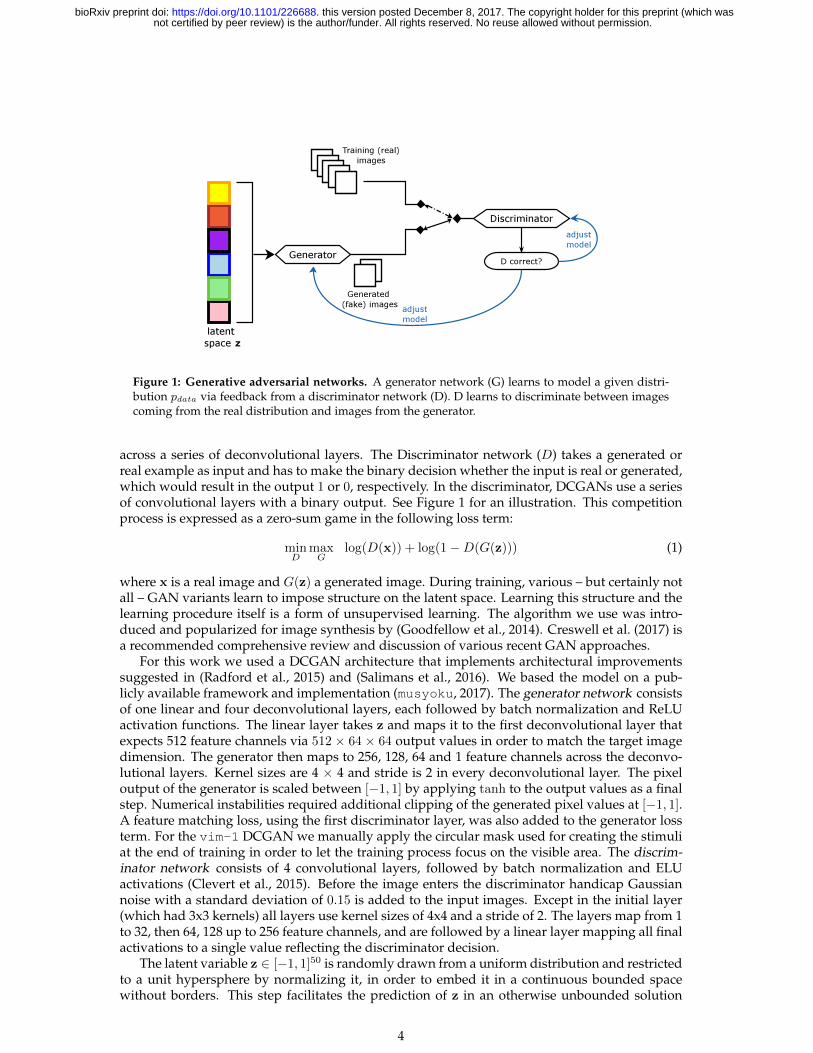
Figure 1: Generative adversarial networks. A generator network (G) learns to model a given distri-bution pdata via feedback from a discriminator network (D). D learns to discriminate between imagescoming from the real distribution and images from the generator.

across a series of deconvolutional layers. The Discriminator network (D) takes a generated orreal example as input and has to make the binary decision whether the input is real or generated,which would result in the output 1 or 0, respectively. In the discriminator, DCGANs use a seriesof convolutional layers with a binary output. See Figure 1 for an illustration. This competitionprocess is expressed as a zero-sum game in the following loss term:

minD

maxG

log(D(x)) + log(1−D(G(z))) (1)

where x is a real image and G(z) a generated image. During training, various – but certainly notall – GAN variants learn to impose structure on the latent space. Learning this structure and thelearning procedure itself is a form of unsupervised learning. The algorithm we use was intro-duced and popularized for image synthesis by (Goodfellow et al., 2014). Creswell et al. (2017) isa recommended comprehensive review and discussion of various recent GAN approaches.

For this work we used a DCGAN architecture that implements architectural improvementssuggested in (Radford et al., 2015) and (Salimans et al., 2016). We based the model on a pub-licly available framework and implementation (musyoku, 2017). The generator network consistsof one linear and four deconvolutional layers, each followed by batch normalization and ReLUactivation functions. The linear layer takes z and maps it to the first deconvolutional layer thatexpects 512 feature channels via 512 × 64 × 64 output values in order to match the target imagedimension. The generator then maps to 256, 128, 64 and 1 feature channels across the deconvo-lutional layers. Kernel sizes are 4 × 4 and stride is 2 in every deconvolutional layer. The pixeloutput of the generator is scaled between [−1, 1] by applying tanh to the output values as a finalstep. Numerical instabilities required additional clipping of the generated pixel values at [−1, 1].A feature matching loss, using the first discriminator layer, was also added to the generator lossterm. For the vim-1 DCGAN we manually apply the circular mask used for creating the stimuliat the end of training in order to let the training process focus on the visible area. The discrim-inator network consists of 4 convolutional layers, followed by batch normalization and ELUactivations (Clevert et al., 2015). Before the image enters the discriminator handicap Gaussiannoise with a standard deviation of 0.15 is added to the input images. Except in the initial layer(which had 3x3 kernels) all layers use kernel sizes of 4x4 and a stride of 2. The layers map from 1to 32, then 64, 128 up to 256 feature channels, and are followed by a linear layer mapping all finalactivations to a single value reflecting the discriminator decision.

The latent variable z ∈ [−1, 1]50 is randomly drawn from a uniform distribution and restrictedto a unit hypersphere by normalizing it, in order to embed it in a continuous bounded spacewithout borders. This step facilitates the prediction of z in an otherwise unbounded solution

4


https://doi.org/10.1101/226688

to the regression problem. For optimizing the weights of the DCGAN we used the Adam opti-mizer (Kingma and Ba, 2014) with default parameters (α = 0.001, β1 = 0.9, β2 = 0.999, ε = 10−8).The learning rate was 10−4 for all networks. We applied gradient clipping with a threshold of 10.

As DCGAN training data we used a downsampled 64 × 64 variant of ImageNet (made avail-able with (Chrabaszcz et al., 2017)) together with the Microsoft COCO dataset6. The image sizeof MS COCO was decreased to 64 × 64 and center-cropped, and images for which this was notpossible due to aspect ratio were removed from the training set. Before entering training allimages were converted to gray scale and contrast-enhanced with imadjust (as in MATLAB),similar to the transformation used in (Kay et al., 2008). The image value range entering trainingwas [−1, 1]. For the vim-1 GAN, again the circular mask was applied. This resulted in approxi-mately 1.500.000 gray scale natural images used for training in total. Note that DCGAN trainingwould usually also work with a lower amount of training data.

The DCGAN on handwritten characters was trained on (in total) 15.000 examples of B, R,A, I, N and S characters from (Van der Maaten, 2009) and (Schomaker and Vuurpijl, 2000). Asthe experiment on the BRAINS dataset should focus on a restricted stimulus domain its DCGANdoes not require more expressive power.

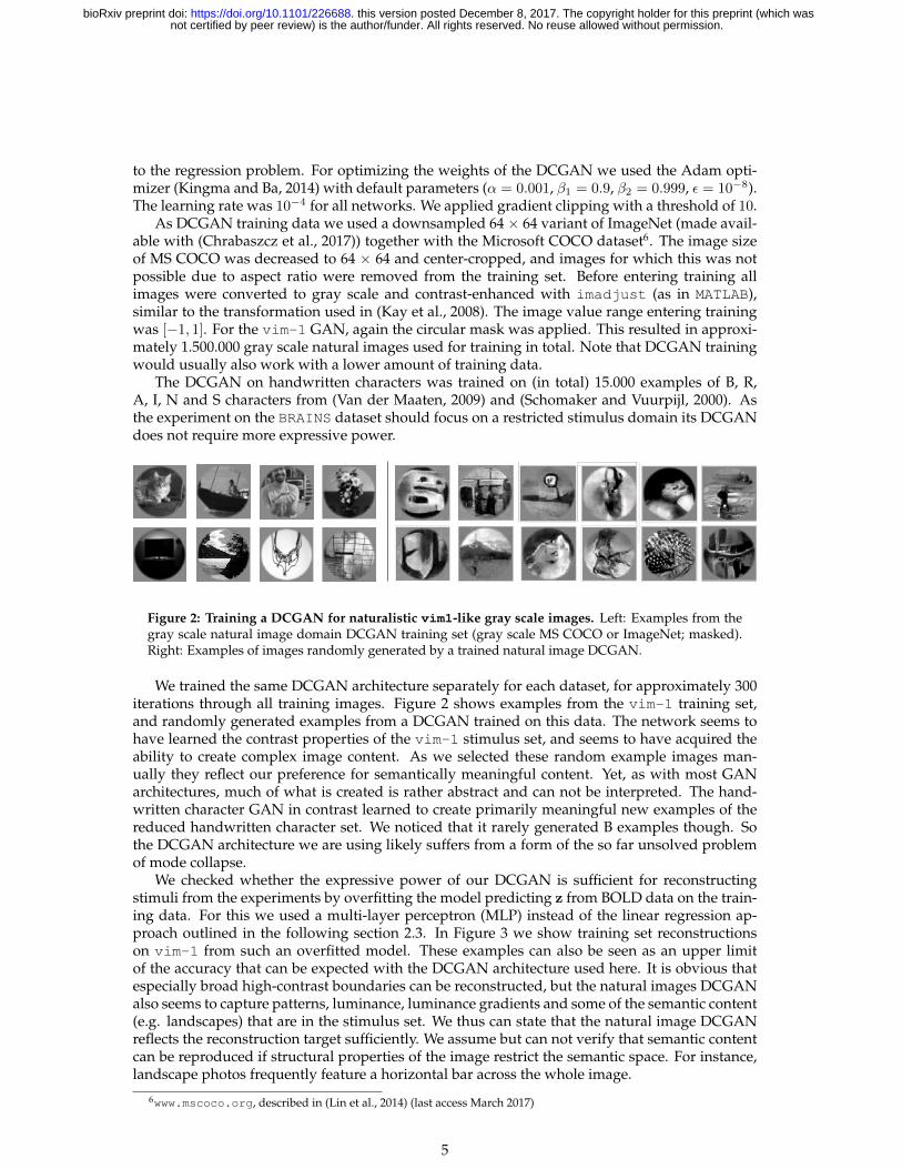
Figure 2: Training a DCGAN for naturalistic vim1-like gray scale images. Left: Examples from thegray scale natural image domain DCGAN training set (gray scale MS COCO or ImageNet; masked).Right: Examples of images randomly generated by a trained natural image DCGAN.

We trained the same DCGAN architecture separately for each dataset, for approximately 300iterations through all training images. Figure 2 shows examples from the vim-1 training set,and randomly generated examples from a DCGAN trained on this data. The network seems tohave learned the contrast properties of the vim-1 stimulus set, and seems to have acquired theability to create complex image content. As we selected these random example images man-ually they reflect our preference for semantically meaningful content. Yet, as with most GANarchitectures, much of what is created is rather abstract and can not be interpreted. The hand-written character GAN in contrast learned to create primarily meaningful new examples of thereduced handwritten character set. We noticed that it rarely generated B examples though. Sothe DCGAN architecture we are using likely suffers from a form of the so far unsolved problemof mode collapse.

We checked whether the expressive power of our DCGAN is sufficient for reconstructingstimuli from the experiments by overfitting the model predicting z from BOLD data on the train-ing data. For this we used a multi-layer perceptron (MLP) instead of the linear regression ap-proach outlined in the following section 2.3. In Figure 3 we show training set reconstructionson vim-1 from such an overfitted model. These examples can also be seen as an upper limitof the accuracy that can be expected with the DCGAN architecture used here. It is obvious thatespecially broad high-contrast boundaries can be reconstructed, but the natural images DCGANalso seems to capture patterns, luminance, luminance gradients and some of the semantic content(e.g. landscapes) that are in the stimulus set. We thus can state that the natural image DCGANreflects the reconstruction target sufficiently. We assume but can not verify that semantic contentcan be reproduced if structural properties of the image restrict the semantic space. For instance,landscape photos frequently feature a horizontal bar across the whole image.

6www.mscoco.org, described in (Lin et al., 2014) (last access March 2017)

5


https://doi.org/10.1101/226688

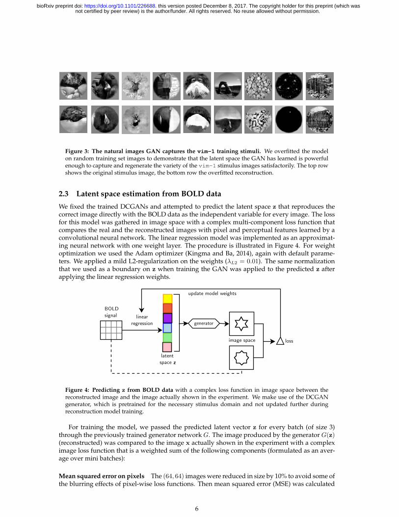
Figure 3: The natural images GAN captures the vim-1 training stimuli. We overfitted the modelon random training set images to demonstrate that the latent space the GAN has learned is powerfulenough to capture and regenerate the variety of the vim-1 stimulus images satisfactorily. The top rowshows the original stimulus image, the bottom row the overfitted reconstruction.

2.3 Latent space estimation from BOLD data

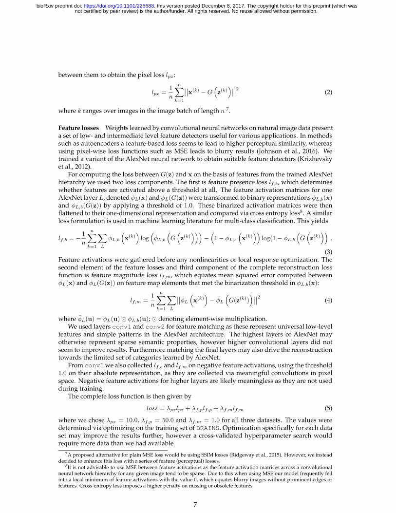
We fixed the trained DCGANs and attempted to predict the latent space z that reproduces thecorrect image directly with the BOLD data as the independent variable for every image. The lossfor this model was gathered in image space with a complex multi-component loss function thatcompares the real and the reconstructed images with pixel and perceptual features learned by aconvolutional neural network. The linear regression model was implemented as an approximat-ing neural network with one weight layer. The procedure is illustrated in Figure 4. For weightoptimization we used the Adam optimizer (Kingma and Ba, 2014), again with default parame-ters. We applied a mild L2-regularization on the weights (λL2 = 0.01). The same normalizationthat we used as a boundary on z when training the GAN was applied to the predicted z afterapplying the linear regression weights.

Figure 4: Predicting z from BOLD data with a complex loss function in image space between thereconstructed image and the image actually shown in the experiment. We make use of the DCGANgenerator, which is pretrained for the necessary stimulus domain and not updated further duringreconstruction model training.

For training the model, we passed the predicted latent vector z for every batch (of size 3)through the previously trained generator network G. The image produced by the generator G(z)(reconstructed) was compared to the image x actually shown in the experiment with a compleximage loss function that is a weighted sum of the following components (formulated as an aver-age over mini batches):

Mean squared error on pixels The (64, 64) images were reduced in size by 10% to avoid some ofthe blurring effects of pixel-wise loss functions. Then mean squared error (MSE) was calculated

6


https://doi.org/10.1101/226688

between them to obtain the pixel loss lpx:

lpx =1

n

n∑k=1

∣∣∣∣x(k) −G(z(k)

)∣∣∣∣2 (2)

where k ranges over images in the image batch of length n 7.

Feature losses Weights learned by convolutional neural networks on natural image data presenta set of low- and intermediate level feature detectors useful for various applications. In methodssuch as autoencoders a feature-based loss seems to lead to higher perceptual similarity, whereasusing pixel-wise loss functions such as MSE leads to blurry results (Johnson et al., 2016). Wetrained a variant of the AlexNet neural network to obtain suitable feature detectors (Krizhevskyet al., 2012).

For computing the loss between G(z) and x on the basis of features from the trained AlexNethierarchy we used two loss components. The first is feature presence loss lf,b, which determineswhether features are activated above a threshold at all. The feature activation matrices for oneAlexNet layerL, denoted φL(x) and φL(G(z)) were transformed to binary representations φL,b(x)and φL,b(G(z)) by applying a threshold of 1.0. These binarized activation matrices were thenflattened to their one-dimensional representation and compared via cross entropy loss8. A similarloss formulation is used in machine learning literature for multi-class classification. This yields

lf,b = − 1

n

n∑k=1

∑L

φL,b

(x(k)

)log(φL,b

(G(z(k)

)))−(

1− φL,b

(x(k)

))log(1− φL,b

(G(z(k)

)).

(3)Feature activations were gathered before any nonlinearities or local response optimization. Thesecond element of the feature losses and third component of the complete reconstruction lossfunction is feature magnitude loss lf,m, which equates mean squared error computed betweenφL(x) and φL(G(z)) on feature map elements that met the binarization threshold in φL,b(x):

lf,m =1

n

n∑k=1

∑L

∣∣∣∣φL (x(k))− φL

(G(z(k))

)∣∣∣∣2 (4)

where φL(u) = φL(u)� φL,b(u); � denoting element-wise multiplication.We used layers conv1 and conv2 for feature matching as these represent universal low-level

features and simple patterns in the AlexNet architecture. The highest layers of AlexNet mayotherwise represent sparse semantic properties, however higher convolutional layers did notseem to improve results. Furthermore matching the final layers may also drive the reconstructiontowards the limited set of categories learned by AlexNet.

From conv1we also collected lf,b and lf,m on negative feature activations, using the threshold1.0 on their absolute representation, as they are collected via meaningful convolutions in pixelspace. Negative feature activations for higher layers are likely meaningless as they are not usedduring training.

The complete loss function is then given by

loss = λpxlpx + λf,plf,p + λf,mlf,m (5)

where we chose λpx = 10.0, λf,p = 50.0 and λf,m = 1.0 for all three datasets. The values weredetermined via optimizing on the training set of BRAINS. Optimization specifically for each dataset may improve the results further, however a cross-validated hyperparameter search wouldrequire more data than we had available.

7A proposed alternative for plain MSE loss would be using SSIM losses (Ridgeway et al., 2015). However, we insteaddecided to enhance this loss with a series of feature (perceptual) losses.

8It is not advisable to use MSE between feature activations as the feature activation matrices across a convolutionalneural network hierarchy for any given image tend to be sparse. Due to this when using MSE our model frequently fellinto a local minimum of feature activations with the value 0, which equates blurry images without prominent edges orfeatures. Cross-entropy loss imposes a higher penalty on missing or obsolete features.

7


https://doi.org/10.1101/226688

Feature matching networks Feature matching requires a universal set of image descriptors thatfrequently occur in our chosen natural images pdata. To obtain these descriptors we trained avariant of AlexNet (Krizhevsky et al., 2012), with one input channel and 5 × 5 kernels in thefirst (conv1) layer on the 64 × 64 grayscale ImageNet data described before. The model wastrained towards classifying the standard set of ImageNet categories. We used this network forvim-1 and Generic Object Decoding, ignoring potential redundancy of features extractedfrom the mask in the former. For the BRAINS data set we again trained an AlexNet architecture.In this case we trained on all 40.000 examples of 36 handwritten digit and character classes from(Van der Maaten, 2009) and (Schomaker and Vuurpijl, 2000) in order to obtain a universal set ofimage descriptors for the handwriting domain.

Reconstruction variability One inherent disadvantage of training models with random compo-nents, such as randomly initialized weights or stochastic gradient descent (e.g. neural networks)is the variability of the results, due to different local minima the model will converge to. Further-more, in the case of GANs small shifts in the predicted latent space can result in well-perceivablechanges in the generated image. We observed this behaviour, which resulted in the model findingdifferent ways to reconstruct certain images, reconstructing different features of images, or notfinding a recognizable reconstruction at all for an image that could be reconstructed in previousmodels. This variability is demonstrated in Figure 8. We attempted to counteract these effectswhen obtaining final reconstructions with a simple ensemble model: We averaged the predictedz over 15 independent training runs, normalizing z to the unit hypersphere again after this.

The feature matching networks, the natural images GAN and the predictive model for z haveall been implemented in the Chainer framework for neural networks (Tokui et al., 2015)9.

3 Results

Using the outlined methods and parameters we obtained a set of validation set reconstructionsfor each data set, out of which we show examples of reconstructed images and failure cases in thefollowing. We proceeded with a quantitative behavioural evaluation of overall recognizability onthese sets.

3.1 Reconstruction examples

3.1.1 Sample reconstructions on BRAINS

reconstructed preserved features failure cases

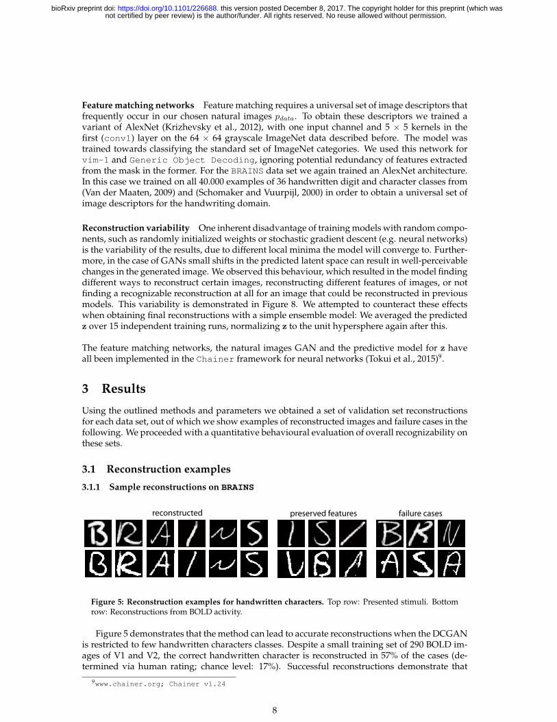
Figure 5: Reconstruction examples for handwritten characters. Top row: Presented stimuli. Bottomrow: Reconstructions from BOLD activity.

Figure 5 demonstrates that the method can lead to accurate reconstructions when the DCGANis restricted to few handwritten characters classes. Despite a small training set of 290 BOLD im-ages of V1 and V2, the correct handwritten character is reconstructed in 57% of the cases (de-termined via human rating; chance level: 17%). Successful reconstructions demonstrate that

9www.chainer.org; Chainer v1.24

8


https://doi.org/10.1101/226688

the model is also capable of reconstructing structural features such as position and curvature oflines. When character classes could not be reconstructed frequently such structural similaritiesremained. As mentioned before, the underlying handwritten character DCGAN had difficultiesgenerating examples of B, and the reconstruction model also failed to reconstruct a B stimulus in9 out of 12 cases.

3.1.2 Sample reconstructions on vim-1

identifiable preserved features failure cases

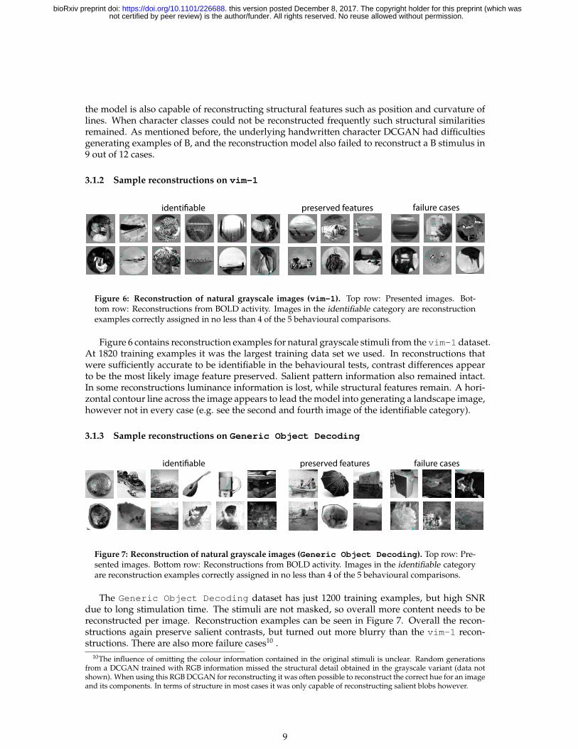
Figure 6: Reconstruction of natural grayscale images (vim-1). Top row: Presented images. Bot-tom row: Reconstructions from BOLD activity. Images in the identifiable category are reconstructionexamples correctly assigned in no less than 4 of the 5 behavioural comparisons.

Figure 6 contains reconstruction examples for natural grayscale stimuli from the vim-1 dataset.At 1820 training examples it was the largest training data set we used. In reconstructions thatwere sufficiently accurate to be identifiable in the behavioural tests, contrast differences appearto be the most likely image feature preserved. Salient pattern information also remained intact.In some reconstructions luminance information is lost, while structural features remain. A hori-zontal contour line across the image appears to lead the model into generating a landscape image,however not in every case (e.g. see the second and fourth image of the identifiable category).

3.1.3 Sample reconstructions on Generic Object Decoding

identifiable preserved features failure cases

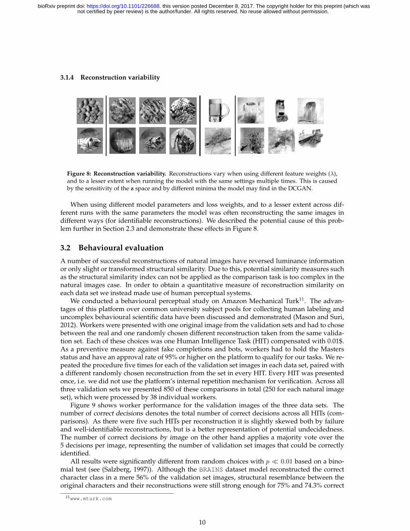
Figure 7: Reconstruction of natural grayscale images (Generic Object Decoding). Top row: Pre-sented images. Bottom row: Reconstructions from BOLD activity. Images in the identifiable categoryare reconstruction examples correctly assigned in no less than 4 of the 5 behavioural comparisons.

The Generic Object Decoding dataset has just 1200 training examples, but high SNRdue to long stimulation time. The stimuli are not masked, so overall more content needs to bereconstructed per image. Reconstruction examples can be seen in Figure 7. Overall the recon-structions again preserve salient contrasts, but turned out more blurry than the vim-1 recon-structions. There are also more failure cases10 .

10The influence of omitting the colour information contained in the original stimuli is unclear. Random generationsfrom a DCGAN trained with RGB information missed the structural detail obtained in the grayscale variant (data notshown). When using this RGB DCGAN for reconstructing it was often possible to reconstruct the correct hue for an imageand its components. In terms of structure in most cases it was only capable of reconstructing salient blobs however.

9


https://doi.org/10.1101/226688

3.1.4 Reconstruction variability

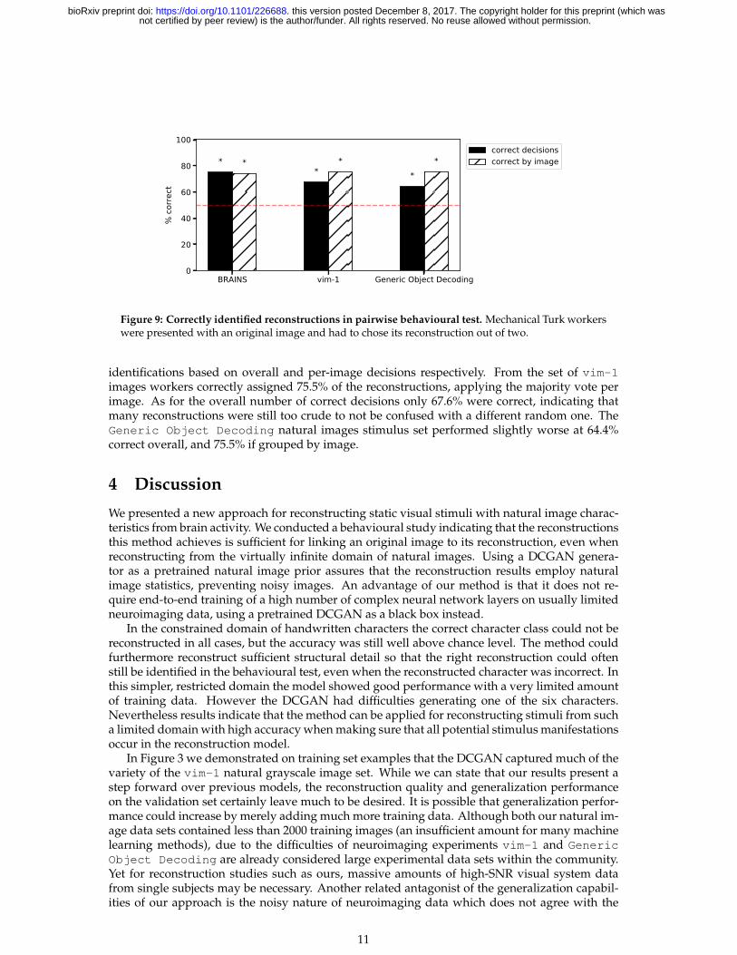
Figure 8: Reconstruction variability. Reconstructions vary when using different feature weights (λ),and to a lesser extent when running the model with the same settings multiple times. This is causedby the sensitivity of the z space and by different minima the model may find in the DCGAN.

When using different model parameters and loss weights, and to a lesser extent across dif-ferent runs with the same parameters the model was often reconstructing the same images indifferent ways (for identifiable reconstructions). We described the potential cause of this prob-lem further in Section 2.3 and demonstrate these effects in Figure 8.

3.2 Behavioural evaluation

A number of successful reconstructions of natural images have reversed luminance informationor only slight or transformed structural similarity. Due to this, potential similarity measures suchas the structural similarity index can not be applied as the comparison task is too complex in thenatural images case. In order to obtain a quantitative measure of reconstruction similarity oneach data set we instead made use of human perceptual systems.

We conducted a behavioural perceptual study on Amazon Mechanical Turk11. The advan-tages of this platform over common university subject pools for collecting human labeling anduncomplex behavioural scientific data have been discussed and demonstrated (Mason and Suri,2012). Workers were presented with one original image from the validation sets and had to chosebetween the real and one randomly chosen different reconstruction taken from the same valida-tion set. Each of these choices was one Human Intelligence Task (HIT) compensated with 0.01$.As a preventive measure against fake completions and bots, workers had to hold the Mastersstatus and have an approval rate of 95% or higher on the platform to qualify for our tasks. We re-peated the procedure five times for each of the validation set images in each data set, paired witha different randomly chosen reconstruction from the set in every HIT. Every HIT was presentedonce, i.e. we did not use the platform’s internal repetition mechanism for verification. Across allthree validation sets we presented 850 of these comparisons in total (250 for each natural imageset), which were processed by 38 individual workers.

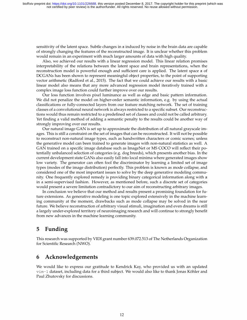
Figure 9 shows worker performance for the validation images of the three data sets. Thenumber of correct decisions denotes the total number of correct decisions across all HITs (com-parisons). As there were five such HITs per reconstruction it is slightly skewed both by failureand well-identifiable reconstructions, but is a better representation of potential undecidedness.The number of correct decisions by image on the other hand applies a majority vote over the5 decisions per image, representing the number of validation set images that could be correctlyidentified.

All results were significantly different from random choices with p � 0.01 based on a bino-mial test (see (Salzberg, 1997)). Although the BRAINS dataset model reconstructed the correctcharacter class in a mere 56% of the validation set images, structural resemblance between theoriginal characters and their reconstructions were still strong enough for 75% and 74.3% correct

11www.mturk.com

10


https://doi.org/10.1101/226688

BRAINS vim-1 Generic Object Decoding0

20

40

60

80

100

% c

orre

ct*

* ** * *

correct decisionscorrect by image

Figure 9: Correctly identified reconstructions in pairwise behavioural test. Mechanical Turk workerswere presented with an original image and had to chose its reconstruction out of two.

identifications based on overall and per-image decisions respectively. From the set of vim-1images workers correctly assigned 75.5% of the reconstructions, applying the majority vote perimage. As for the overall number of correct decisions only 67.6% were correct, indicating thatmany reconstructions were still too crude to not be confused with a different random one. TheGeneric Object Decoding natural images stimulus set performed slightly worse at 64.4%correct overall, and 75.5% if grouped by image.

4 Discussion

We presented a new approach for reconstructing static visual stimuli with natural image charac-teristics from brain activity. We conducted a behavioural study indicating that the reconstructionsthis method achieves is sufficient for linking an original image to its reconstruction, even whenreconstructing from the virtually infinite domain of natural images. Using a DCGAN genera-tor as a pretrained natural image prior assures that the reconstruction results employ naturalimage statistics, preventing noisy images. An advantage of our method is that it does not re-quire end-to-end training of a high number of complex neural network layers on usually limitedneuroimaging data, using a pretrained DCGAN as a black box instead.

In the constrained domain of handwritten characters the correct character class could not bereconstructed in all cases, but the accuracy was still well above chance level. The method couldfurthermore reconstruct sufficient structural detail so that the right reconstruction could oftenstill be identified in the behavioural test, even when the reconstructed character was incorrect. Inthis simpler, restricted domain the model showed good performance with a very limited amountof training data. However the DCGAN had difficulties generating one of the six characters.Nevertheless results indicate that the method can be applied for reconstructing stimuli from sucha limited domain with high accuracy when making sure that all potential stimulus manifestationsoccur in the reconstruction model.

In Figure 3 we demonstrated on training set examples that the DCGAN captured much of thevariety of the vim-1 natural grayscale image set. While we can state that our results present astep forward over previous models, the reconstruction quality and generalization performanceon the validation set certainly leave much to be desired. It is possible that generalization perfor-mance could increase by merely adding much more training data. Although both our natural im-age data sets contained less than 2000 training images (an insufficient amount for many machinelearning methods), due to the difficulties of neuroimaging experiments vim-1 and GenericObject Decoding are already considered large experimental data sets within the community.Yet for reconstruction studies such as ours, massive amounts of high-SNR visual system datafrom single subjects may be necessary. Another related antagonist of the generalization capabil-ities of our approach is the noisy nature of neuroimaging data which does not agree with the

11


https://doi.org/10.1101/226688

sensitivity of the latent space. Subtle changes in z induced by noise in the brain data are capableof strongly changing the features of the reconstructed image. It is unclear whether this problemwould remain in an experiment with much larger amounts of data with high quality.

Also, we achieved our results with a linear regression model. This linear relation promisesinterpretability of the relations between the latent space and brain representations, when thereconstruction model is powerful enough and sufficient care is applied. The latent space z ofDCGANs has been shown to represent meaningful object properties, to the point of supportingvector arithmetic (Radford et al., 2015). The fact that we could achieve our results with a basiclinear model also means that any more advanced regression model iteratively trained with acomplex image loss function could further improve over our results.

Our loss function involves pixel luminance as well as edge and basic pattern information.We did not penalize the model on higher-order semantic information, e.g. by using the actualclassifications or fully-connected layers from our feature matching network. The set of trainingclasses of a convolutional neural network is always restricted to a specific subset. Our reconstruc-tions would thus remain restricted to a predefined set of classes and could not be called arbitrary.Yet finding a valid method of adding a semantic penalty to the results could be another way ofstrongly improving over our results.

Our natural image GAN is set up to approximate the distribution of all natural grayscale im-ages. This is still a constraint on the set of images that can be reconstructed. It will not be possibleto reconstruct non-natural image types, such as handwritten characters or comic scenes; unlessthe generative model can been trained to generate images with non-natural statistics as well. AGAN trained on a specific image database such as ImageNet or MS COCO will reflect their po-tentially unbalanced selection of categories (e.g. dog breeds), which presents another bias. In thecurrent development state GANs also easily fall into local minima where generated images showlow variety. The generator can often fool the discriminator by learning a limited set of imagetypes (modes of the image distribution) perfectly. This problem is known as mode collapse, andconsidered one of the most important issues to solve by the deep generative modeling commu-nity. One frequently explored remedy is providing binary categorical information along with zin a semi-supervised fashion. However, as mentioned before, such a discrete set of categorieswould present a severe limitation contradictory to our aim of reconstructing arbitrary images.

In conclusion we believe that our method and results present a promising foundation for fu-ture extensions. As generative modeling is one topic explored extensively in the machine learn-ing community at the moment, drawbacks such as mode collapse may be solved in the nearfuture. We believe reconstruction of arbitrary visual stimuli, imagination and even dreams is stilla largely under-explored territory of neuroimaging research and will continue to strongly benefitfrom new advances in the machine learning community.

5 Funding

This research was supported by VIDI grant number 639.072.513 of The Netherlands Organizationfor Scientific Research (NWO).

6 Acknowledgements

We would like to express our gratitude to Kendrick Kay, who provided us with an updatedvim-1 dataset, including data for a third subject. We would also like to thank Jonas Kohler andPaul Zhutovsky for discussions.

12


https://doi.org/10.1101/226688

References

Chang, L. and Tsao, D. Y. (2017). The code for facial identity in the primate brain. Cell,169(6):1013–1028.

Chrabaszcz, P., Loshchilov, I., and Hutter, F. (2017). A downsampled variant of ImageNet as analternative to the CIFAR datasets. arXiv preprint arXiv:1707.08819.

Clevert, D.-A., Unterthiner, T., and Hochreiter, S. (2015). Fast and accurate deep networklearning by exponential linear units (ELUs). arXiv preprint arXiv:1511.07289.

Creswell, A. P. N., White, T., Dumoulin, V., Arulkumaran, K., Sengupta, B., and Bharath, A. A.(2017). Generative adversarial networks: An overview. arXiv preprint arXiv: 1710.07035.

Deng, J., Dong, W., Socher, R., Li, L.-J., Li, K., and Fei-Fei, L. (2009). ImageNet: A large-scalehierarchical image database. In IEEE Conference on Computer Vision and Pattern Recognition(CVPR) 2009, pages 248–255.

Du, C., Du, C., and He, H. (2017). Sharing deep generative representation for perceived imagereconstruction from human brain activity. In International Joint Conference on Neural Networks(IJCNN) 2017, pages 1049–1056.

Goodfellow, I., Pouget-Abadie, J., Mirza, M., Xu, B., Warde-Farley, D., Ozair, S., Courville, A.,and Bengio, Y. (2014). Generative adversarial nets. In Advances in Neural Information ProcessingSystems (NIPS) 2014, pages 2672–2680.

Gucluturk, Y., Guclu, U., Seeliger, K., Bosch, S., van Lier, R., and van Gerven, M. A. (2017).Reconstructing perceived faces from brain activations with deep adversarial neural decoding.In Advances in Neural Information Processing Systems (NIPS) 2017, pages 4249–4260.

Guclu, U. and van Gerven, M. (2013). Unsupervised learning of features for bayesian decodingin functional magnetic resonance imaging. In 22nd annual Belgian-Dutch Conference on MachineLearning (BeNeLearn) 2013.

Hanke, M., Halchenko, Y. O., Sederberg, P. B., Hanson, S. J., Haxby, J. V., and Pollmann, S. (2009).PyMVPA: A python toolbox for multivariate pattern analysis of fMRI data. Neuroinformatics,7(1):37–53.

Haxby, J. V. (2001). Distributed and overlapping representations of faces and objects in ventraltemporal cortex. Science, 293(5539):2425–2430.

Haxby, J. V., Guntupalli, J. S., Connolly, A. C., Halchenko, Y. O., Conroy, B. R., Gobbini, M. I.,Hanke, M., and Ramadge, P. J. (2011). A common, high-dimensional model of therepresentational space in human ventral temporal cortex. Neuron, 72(2):404–416.

Haynes, J.-D. (2015). A primer on pattern-based approaches to fMRI: Principles, pitfalls, andperspectives. Neuron, 87(2):257–270.

Horikawa, T. and Kamitani, Y. (2017). Generic decoding of seen and imagined objects usinghierarchical visual features. Nature Communications, 8.

Huth, A. G., Lee, T., Nishimoto, S., Bilenko, N. Y., Vu, A. T., and Gallant, J. L. (2016). Decodingthe semantic content of natural movies from human brain activity. Frontiers in SystemsNeuroscience, 10(81).

Johnson, J., Alahi, A., and Fei-Fei, L. (2016). Perceptual losses for real-time style transfer andsuper-resolution. In European Conference on Computer Vision (ECCV) 2016, pages 694–711.

Kamitani, Y. and Tong, F. (2005). Decoding the visual and subjective contents of the humanbrain. Nature Neuroscience, 8(5):679–685.

13


https://doi.org/10.1101/226688

Kay, K. N., Naselaris, T., Prenger, R. J., and Gallant, J. L. (2008). Identifying natural images fromhuman brain activity. Nature, 452(7185):352–355.

Kingma, D. P. and Ba, J. (2014). Adam: A method for stochastic optimization. arXiv preprintarXiv:1412.6980.

Krizhevsky, A., Sutskever, I., and Hinton, G. E. (2012). ImageNet classification with deepconvolutional neural networks. In Advances in Neural Information Processing Systems (NIPS)2012, pages 1097–1105.

Lin, T.-Y., Maire, M., Belongie, S., Hays, J., Perona, P., Ramanan, D., Dollar, P., and Zitnick, C. L.(2014). Microsoft COCO: Common Objects in Context. In European Conference on ComputerVision (ECCV) 2014, pages 740–755.

Mason, W. and Suri, S. (2012). Conducting behavioral research on Amazon’s Mechanical Turk.Behavior Research Methods, 44(1):1–23.

Miyawaki, Y., Uchida, H., Yamashita, O., Sato, M., Morito, Y., Tanabe, H. C., Sadato, N., andKamitani, Y. (2008). Visual image reconstruction from human brain activity using acombination of multiscale local image decoders. Neuron, 60(5):915–929.

musyoku (2017). Code for the paper: Improved techniques for training GANs.github.com/musyoku/improved-gan. Commit: ba1e09f (--short).

Naselaris, T., Prenger, R. J., Kay, K. N., Oliver, M., and Gallant, J. L. (2009). Bayesianreconstruction of natural images from human brain activity. Neuron, 63(6):902–915.

Nishimoto, S., Vu, A. T., Naselaris, T., Benjamini, Y., Yu, B., and Gallant, J. L. (2011).Reconstructing visual experiences from brain activity evoked by natural movies. CurrentBiology, 21(19):1641–1646.

Parthasarathy, N., Batty, E., Falcon, W., Rutten, T., Rajpal, M., Chichilnisky, E., and Paninski, L.(2017). Neural networks for efficient bayesian decoding of natural images from retinalneurons. In Advances in Neural Information Processing Systems (NIPS) 2017, pages 6437–6448.

Radford, A., Metz, L., and Chintala, S. (2015). Unsupervised representation learning with deepconvolutional generative adversarial networks. arXiv preprint arXiv:1511.06434.

Ridgeway, K., Snell, J., Roads, B., Zemel, R. S., and Mozer, M. C. (2015). Learning to generateimages with perceptual similarity metrics. arXiv preprint arxiv:1511.06409.

Salimans, T., Goodfellow, I., Zaremba, W., Cheung, V., Radford, A., and Chen, X. (2016).Improved techniques for training GANs. In Advances in Neural Information Processing Systems(NIPS) 2016, pages 2234–2242.

Salzberg, S. L. (1997). On comparing classifiers: Pitfalls to avoid and a recommended approach.Data Mining and Knowledge Discovery, 328:317–328.

Schoenmakers, S., Barth, M., Heskes, T., and van Gerven, M. A. J. (2013). Linear reconstructionof perceived images from human brain activity. NeuroImage, 83:951–961.

Schoenmakers, S., Guclu, U., van Gerven, M. A. J., and Heskes, T. (2015). Gaussian mixturemodels and semantic gating improve reconstructions from human brain activity. Frontiers inComputational Neuroscience, 8:173.

Schomaker, L. and Vuurpijl, L. (2000). Forensic writer identification: A benchmark data set anda comparison of two systems [internal report for the Netherlands Forensic Institute].

Stanley, G. B., Li, F. F., and Dan, Y. (1999). Reconstruction of natural scenes from ensembleresponses in the lateral geniculate nucleus. Journal of Neuroscience, 19(18):8036–8042.

14


https://doi.org/10.1101/226688

Thirion, B., Duchesnay, E., Hubbard, E., Dubois, J., Poline, J. B., Lebihan, D., and Dehaene, S.(2006). Inverse retinotopy: Inferring the visual content of images from brain activationpatterns. NeuroImage, 33(4):1104–1116.

Tokui, S., Oono, K., Hido, S., and Clayton, J. (2015). Chainer: A next-generation open sourceframework for deep learning. In Workshop on Machine Learning Systems (LearningSys) duringAdvances in Neural Information Processing Systems (NIPS) 2015.

Van der Maaten, L. (2009). A new benchmark dataset for handwritten character recognition.Tilburg University.

15


https://doi.org/10.1101/226688

generative adversarial networks for reconstructing natural ...€¦ · generative adversarial...

Documents