generative lattice structures for 3d printing

Generative Lattice Structures for 3D Printing

Ruiqi ChenDepartment of Aeronautics and Astronautics

Stanford [email protected]

Category: generative modeling

1 Introduction

Additive manufacturing (AM) has allowed geometries that were once impossible to manufacture tobe created quickly. However, as AM technologies advance, there is a need to develop design toolsthat can keep up with AM’s capabilities. Recently, there has been significant interest in using levelset methods and implicit surface modeling to create novel geometries, infills, and organic lattice-likestructures. These structures are typically generated based on trigonometric implicit surface equationsto ensure periodicity [1]. In this work, we use a generative adversarial network (GAN) to discover newrepresentations for modeling lattice structures that may lead to new, undiscovered lattice structuresthat go beyond existing trigonometric implicit surface representations.

2 Dataset

The dataset consists of 31981 synthesized boolean voxel grids that represent periodic implicit surfacelattices. Specifically, they are synthesized using a trigonometric implicit surface equation of the form

f(x, y, z) =

(c+

N∑i=1

(wipi(πhix)qi(πkiy)ri(πliz))

)2

− t2 = 0

c ∈ Rwi ∈ RN ∈ N+

p, q, r ∈ {sin, cos}h, k, l ∈ N0

t ∈ R

(1)

A physical interpretation of Equation 1 is that it uses two trigonometric functions, sine and cosine,to generate periodic surfaces along the Cartesian coordinates. The factor of π is used to ensureperiodicity in the unit cube [−1, 1]3. Equation 1 is general enough to represent all of the commontriply periodic level set approximations such as Schwarz-P, diamond (Schwarz-D), and Schoen’sgyroid [2]. It is also used by researchers and additive manufacturing companies such as nTopologyand Carbon3D to design and manufacture real products [3, 4, 5, 6]. Thus, even though the dataset issynthetic, it is representative of real world lattice structures.

Synthetic data is generated using Equation 1 by first evaluating it in the domain [−1, 1]3 using a32 × 32 × 32 array in NumPy [7]. Positive array values represent empty space while negativevalues represent solid material (and thus the value zero, also known as the zero level set, represents

CS230: Deep Learning, Spring 2020, Stanford University, CA. (LATEXtemplate borrowed from NIPS 2017.)

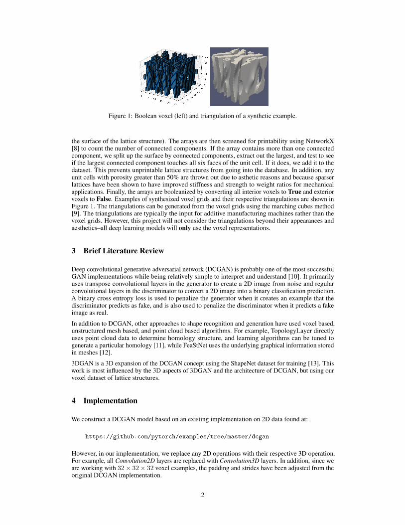
Figure 1: Boolean voxel (left) and triangulation of a synthetic example.

the surface of the lattice structure). The arrays are then screened for printability using NetworkX[8] to count the number of connected components. If the array contains more than one connectedcomponent, we split up the surface by connected components, extract out the largest, and test to seeif the largest connected component touches all six faces of the unit cell. If it does, we add it to thedataset. This prevents unprintable lattice structures from going into the database. In addition, anyunit cells with porosity greater than 50% are thrown out due to asthetic reasons and because sparserlattices have been shown to have improved stiffness and strength to weight ratios for mechanicalapplications. Finally, the arrays are booleanized by converting all interior voxels to True and exteriorvoxels to False. Examples of synthesized voxel grids and their respective triangulations are shown inFigure 1. The triangulations can be generated from the voxel grids using the marching cubes method[9]. The triangulations are typically the input for additive manufacturing machines rather than thevoxel grids. However, this project will not consider the triangulations beyond their appearances andaesthetics–all deep learning models will only use the voxel representations.

3 Brief Literature Review

Deep convolutional generative adversarial network (DCGAN) is probably one of the most successfulGAN implementations while being relatively simple to interpret and understand [10]. It primarilyuses transpose convolutional layers in the generator to create a 2D image from noise and regularconvolutional layers in the discriminator to convert a 2D image into a binary classification prediction.A binary cross entropy loss is used to penalize the generator when it creates an example that thediscriminator predicts as fake, and is also used to penalize the discriminator when it predicts a fakeimage as real.

In addition to DCGAN, other approaches to shape recognition and generation have used voxel based,unstructured mesh based, and point cloud based algorithms. For example, TopologyLayer directlyuses point cloud data to determine homology structure, and learning algorithms can be tuned togenerate a particular homology [11], while FeaStNet uses the underlying graphical information storedin meshes [12].

3DGAN is a 3D expansion of the DCGAN concept using the ShapeNet dataset for training [13]. Thiswork is most influenced by the 3D aspects of 3DGAN and the architecture of DCGAN, but using ourvoxel dataset of lattice structures.

4 Implementation

We construct a DCGAN model based on an existing implementation on 2D data found at:

https://github.com/pytorch/examples/tree/master/dcgan

However, in our implementation, we replace any 2D operations with their respective 3D operation.For example, all Convolution2D layers are replaced with Convolution3D layers. In addition, since weare working with 32× 32× 32 voxel examples, the padding and strides have been adjusted from theoriginal DCGAN implementation.

2

The following are the applicable hyperparameters used by the model:

number of examples: m = 5785

batch size: nbs = 64

image size: nh, nw, nd, nc = 32, 32, 32, 1

number of filters: nf = 64

latent vector size: nz = 100

learning rate: α = 0.0002

adam parameters: β1 = 0.5, β2 = 0.999

(2)

The generator architecture is given by

1. ConvTranspose3d: channels in 100, channels out 256, kernal 4, stride 1

2. BatchNorm3d: eps 1e-5, momentum 0.1

3. ReLU

4. ConvTranspose3d: channels in 256, channels out 128, kernal 4, stride 2, padding 1


6. ReLU



9. ReLU


11. Tanh()

while the discriminator architecture is given by

1. Conv3d: channels in 1, channels out 64, kernal 4, stride 2, padding 1

2. LeakyReLU: negative slope 0.2







9. Conv3d: channels in 256, channels out 1, kernal 4, stride 2

10. Sigmoid()

Because the generator uses a Tanh activation as the last year (with output range [−1, 1]), the inputboolean voxelgrid was converted such that all True values (interior voxels) become −1 and all Falsevalues (exterior values) become +1. This also fits the existing convention that the surface is definedby the zero level set and that interior voxels are negative, which is what the original implicit surfaceequations follow. Implementation is done using PyTorch [14] using Google CoLaboratory platformwith GPUs.

5 Results

Several deepfakes as well as genenerator and discriminator losses are depicted in Figure 3. Both thegenerator and discriminator losses decreased and leveled out after less than 200 iterations (2 epochs)with the default Adam settings. The average porosity of the generated lattices is around 40%, whichis near the average of the training set.

3

5.1 Printability Loss

To improve the quality of the generated lattices, we attempt to enforce printability constraints in theform of additional loss functions. Specifically, the generated lattices should ideally consist of onesingle connected component, the opposing faces should be matching for periodicity reasons, and thedensity of the lattices should be relatively low (e.g. 10-40%) without becoming razor thin. Theseadditional losses, deemed PrintabilityLoss, are only applied to the generator and not the discriminatorin an effort to encourage the generator to produce more realistic lattice structures.

5.1.1 Density Loss

To reduce density, we add a density loss for a single example x defined as

DensityLoss(x) =1(x ≤ 0)

32× 32× 32(3)

This loss physically represents the density of the example and is summed up across all examples. Thenetwork was trained using five epochs but with various amounts of density loss regularization applied.As shown in Table 5.1.1, increasing density loss reduces the density of the generated examples, butwhen λdensity is increased to 0.1, the density increases and the model begins to show instabilities inthe losses (lots of oscillations).

λdensity Average density0 0.4181405639648437

0.001 0.413518066406250.01 0.354081115722656270.1 0.3858355712890625

Two examples of lattices with and without density loss are shown in Figure 4.

5.1.2 Periodicity Loss

To enforce surface periodicity, we note the fact that matching voxels on opposite faces should havethe same signs. A reasonable loss function would be based on taking the exclusive or (XOR) ofopposing faces and summing up the results, but the element-wise XOR operation in PyTorch is notdifferentiable. Instead, we resort to a hack. We take the element-wise product of opposing faces,negate the values, and apply a softplus function. This effectively reduces any negative values (whichare generated by element pairs with the same sign) to zero while keeping the values of positive values(which are generated by element pairs with opposite signs). The surface periodicity loss for a singleexample x is defined as

SurfacePeriodicityLoss(x) =3∑i

∑j∈{front,back}

ln(1 + exp(x[i;0] · x[i;31])) (4)

where x[i;j] refers to the j-th slice of the i-th face on example x. Note that this loss is only applied tosurface voxels as the surface is mainly responsible for maintaining periodicity in a large continuouslattice. Surface voxel images with varying amounts of periodicity loss applied are shown in Figure5. At high periodicity loss values, the generator begins to make all surfaces entirely solid. This isreasonable behavior because as more emphasis is put on periodicity, the generator becomes worse atproducing geometries that fool the discriminator. Increasing the number of epochs from five to tenwhile keeping the periodicity loss at a reasonable level seems to produce better periodicity results, asshown in Figure 6.

5.1.3 Persistent Homology Loss

We attempted to add persistent homology loss to drive the generation towards single connectedcomponent shapes but were unable to due to difficulty in getting a persistent homology package intoCoLaboratory. TopologyLayer seemed the most promising but CoLaboratory could not compile thepackage properly. Alternatives like Ripser were investigated as well but could not be easily ported toPyTorch. This should be a subject of future investigations.

4

Figure 2: Examples of four deep fakes generated by our GAN with density and periodicity lossapplied.

5.2 Finalized Parameter Set

Using all 31981 examples in the dataset, we ran the model with 0.2 density loss and 1e− 4 weightfor periodicity loss for over 5 epochs. Deep fakes generated with these hyperparameters (depicted inFigure 2) show an average density of 33% and have reasonable face periodicity. Figure 2(d) depictsan example of a fake that is not very convincing. The generator and discriminator loss functions,shown in Figure 2, suggest that while the discriminator seems to have converged, the generator isstill rather unstable. However, the generator loss did decrease from 20 to about 15 over the 5 epochs,showing it was able to successfully fool the discriminator in some cases. The biggest impact seemedto be increasing the dataset from the original 5000 to 31981 examples. Specifically, adding examplesfrom multiple connected component lattices but with only the biggest component kept seemed tohelp the GAN generate more convincing lattices, since these lattices cannot be generated directlyfrom the implicit surface equations and requires a postprocessing filtering step.

6 Future Work

The current work utilized an existing 2D DCGAN that was converted to accept 3D boolean voxel gridinputs. The layers only consist of convolutional, transpose convolutional, and batch normalizationlayers. Some aspects of printability constraints were imposed using modified loss functions to controlthe density and surface periodicity of the generated lattices. Increasing the number of examples from5000 to 31981 greatly improved the realism of the generated shapes. However, several aspects thatshould be addressed in future work include:

1. The real examples only contain voxel values of -1 and +1, but the generator produces fakeswith real values. Would using real-valued examples help or hurt the generation?

2. If persistent homology was applied, can it be used to constrain the number of connectedccomponents as well as holes and cavities?

3. Are there any patterns or clusters in the generated lattices? Are they diverse looking or arethey narrow focused? What are the appropriate metrics for evaluating diversity in a set oflattices?

Dataset and Model Availability

The full dataset and CoLaboratory notebook may be found at

https://github.com/rchensix/cs230_public

5

References

[1] Wohlgemuth, M. et al. (2001) Triply periodic bicontinuous cubic microdomain morphologies by symmetries.Macromolecules 34(17):6083-6089

[2] Schoen, A. (1970) Infinite periodic minimal surfaces without self-intersections. National Aeronautics andSpace Administration, 1970.

[3] Yoo, D.J. (2011) Computer-aided porous scaffold design for tissue engineering using triply periodic minimalsurfaces. International Journal of Precision Engineering and Manufacturing 12(1):61-71.

[4] Zhang, L., Feih, S., Daynes, S., Chang, S., Wang, M.Y., Wei, J. & Lu, W.F. (2018) Energy absorptioncharacteristics of metallic triply periodic minimal surface sheet structures under compressive loading. AdditiveManufacturing 23:505-515.

[5] Vlahinos, M. et al. (2019) Whitepaper: Unlocking Advanced Heat Exchanger Design and Simulation withnTop Platform and ANSYS CFX. nTopology

[6] Riddell. (2019) Precision Fit. Riddell

[7] Oliphant, T. et al. (2007) Python for scientific computing. Computing in Science & Engineering 9(3):10-20.

[8] Hagberg, A., Swart, P. & Chult, D.S. (2008) Exploring network structure, dynamics, and function usingNetworkX. Los Alamos National Lab.

[9] Van der Walt, S., Schonberger, J.L., Nunez-Iglesias, J., Boulogne, F., Warner, J.D., Yager, N., Gouillart, E. &Yu, T. (2014) scikit-image: image processing in Python. PeerJ 2:e453.

[10] Radford, A., Metz, L. & Chintala, S. (2015) Unsupervised representation learning with deep convolutionalgenerative adversarial networks. arXiv:1511.06434.

[11] Gabrielsson, R, B. et al. (2019) A topology layer for machine learning. arXiv:1905.12200.

[12] Verma, N. et al. (2018) FeaStNet: Feature-steered graph convolutions for 3D shape analysis. The IEEEConference on Computer Vision and Pattern Recognition: 2598–2606

[13] Wu, J. et al. (2016) Learning a probabilistic latent space of object shapes via 3D generative-adversarialmodeling. 29th Conference on Neural Information Processing Systems (NIPS 2016)

[14] Paszke, A., et al. (2019) PyTorch: An imperative style, high-performance deep learning library. Advancesin Neural Information Processing Systems:8024–8035

6

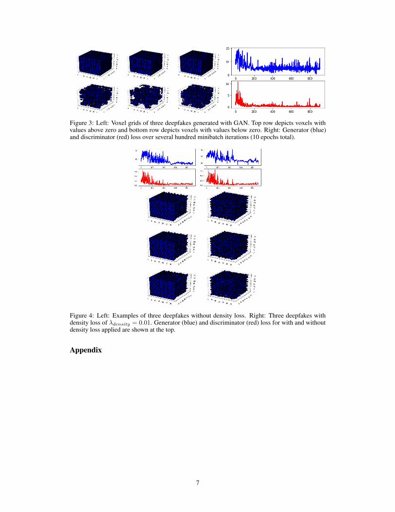
Figure 3: Left: Voxel grids of three deepfakes generated with GAN. Top row depicts voxels withvalues above zero and bottom row depicts voxels with values below zero. Right: Generator (blue)and discriminator (red) loss over several hundred minibatch iterations (10 epochs total).

Figure 4: Left: Examples of three deepfakes without density loss. Right: Three deepfakes withdensity loss of λdensity = 0.01. Generator (blue) and discriminator (red) loss for with and withoutdensity loss applied are shown at the top.

Appendix

7

Figure 5: Opposing faces of a deepfake generated with various levels of periodicity loss. Yellowindicates a positive (exterior) voxel while purple indicates a negative (interior) voxel. At a periodicityloss of 0.001, the generator tries to make the surfaces entirely solid.

Figure 6: Top: Generator (blue) and discriminator (red) loss for model after 10 epochs, showingstrange loss behavior in the generator. Bottom: Opposing faces of a deepfake generated with thismodel. Yellow indicates a positive (exterior) voxel while purple indicates a negative (interior) voxel.The results show the generator does better with matching face voxels compared to the model trainedwith 5 epochs.

8

generative lattice structures for 3d printing

Documents