genetic algorithms - tu dresden · pdf fileannals of operations research 63(1996)339-370 339...

337

Genetic Algorithms

Annals of Operations Research 63(1996)339-370 339

Genetic algorithms for the traveling salesman problem

Jean-Yves Potvin Centre de Recherche sur les Transports, Universitd de Montrgal,

C.P. 6128, Succ. Centre-Ville, Montrdal, Qudbec, Canada H3C 3J7

This paper is a survey of genetic algorithms for the traveling salesman problem. Genetic algorithms are randomized search techniques that simulate some of the processes observed in natural evolution. In this paper, a simple genetic algorithm is introduced, and various extensions are presented to solve the traveling salesman problem. Computational results are also reported for both random and classical problems taken from the operations research literature. Keywords: Traveling salesman problem, genetic algorithms, stochastic search.

1. Introduction

The Traveling Salesman Problem (TSP) is a classical combinatorial optimization problem, which is simple to state but very difficult to solve. The problem is to find the shortest tour through a set of N vertices so that each vertex is visited exactly once. This problem is known to be NP-hard, and cannot be solved exactly in polynomial time.

Many exact and heuristic algorithms have been developed in the field of operations research (OR) to solve this problem. We refer readers to Bodin et al. [5], Lawler et al. [35], Laporte [34] for good overviews of the TSP. In the sections that follow, we briefly introduce the OR problem-solving approaches to the TSP. Then, the genetic algorithms are discussed.

1.1. EXACT ALGORITHMS

The exact algorithms are designed to find the optimal solution to the TSP, that is, the tour of minimal length. They are computationally expensive because they must (implicitly) consider all solutions in order to identify the optimum. These exact algorithms are typically derived from the integer linear programming (ILP) formulation of the TSP

© J.C. Baltzer AG, Science Publishers

340 J.-Y. Potvin, The traveling salesman problem

Minimize ~ , ~ , d i jx i j i j

subject to ~_~ xij = I, i = 1 . . . . . N, J

Z Xij = 1, i

(Xij ) E X, xij : 0 o r 1,

j = l . . . . . N,

where N is the number of. vertices, dij is the distance between vertices i and j , and the xij's are the decision variables: xij is set to 1 when arc ( i , j ) is included in the tour, and 0 otherwise. (xij) E X denotes the set of subtour-breaking constraints that restrict the feasible solutions to those consisting of a single tour.

Although the subtour-breaking constraints can be formulated in many different ways, one very intuitive formulation is

Z Xij <<" S V I - 1 (S V C V; 2 <-Isvl <- N - 2), i,j ~ Sv

where V is the set of all vertices, S v is some subset of V, and [Sv[ is the cardinality of S v. These constraints prohibit subtours, that is, tours on subsets with less than N vertices. If there were such a subtour on some subset of vertices Sv, this subtour would contain I Svt arcs. Consequently, the left-hand side of the inequality would be equal to I Svl , which is greater than I s v l - 1, and the above constraint would be violated for this particular subset. Without the subtour-breaking constraints, the TSP reduces to an assignment problem (AP), and a solution like the one shown in figure 1 would then be feasible.

(b) (

Figure 1. (a) Solving the TSP. (b) Solving the assignment problem.

Branch and bound algorithms are commonly used to find an optimal solution to the TSP, and the above AP-relaxation is useful to generate good lower bounds on

J.-Y. Potvin, The traveling salesman problem 341

the optimal value. This is true in particular for asymmetric problems, where dij ~ dji for some i,j. For symmetric problems, like the Euclidean TSP (ETSP), the AP- solutions often contain many subtours on two vertices. Consequently, these problems are better addressed by specialized algorithms that can exploit their particular structure. For instance, a specific ILP formulation can be derived for the symmetric problem which allows for relaxations that provide sharp lower bounds (i.e., the well-known one-tree relaxation [25]).

It is worth noting that problems with a few hundred vertices can now be routinely solved to optimality. Moreover, instances involving more than 2000 vertices have been recently addressed. For example, the optimal solution to a symmetric problem with 2392 vertices was found after two hours and forty minutes of computation time on a powerful vector computer, the IBM 3090/600 (Padberg and Rinaldi [50, 51 ]). On the other hand, a classical problem with 532 vertices took five hours on the same machine, indicating that the size of the problem is not the only determining factor for computation time.

We refer the interested reader to [34] for a good account of the state-of-the- art in exact algorithms.

1.2. HEURISTIC ALGORITHMS

Running an exact algorithm for hours on a powerful computer may not be very cost-effective if a solution, within a few percent of the optimum, can be found quickly on a small microcomputer. Accordingly, heuristic or approximate algorithms are often preferred to exact algorithms for solving the large TSPs that occur in practice (e.g., drilling problems). Generally speaking, TSP heuristics can be classified as tour construction procedures, tour improvement procedures, and composite procedures, which are based on both construction and improvement techniques.

(a) Construction procedures. The best known procedures in this class gradually build a tour by selecting each vertex in turn and by inserting them one by one into the current tour. Various measures are used for selecting the next vertex and for identifying the best insertion place, like the proximity to the current tour and the minimum detour (Rosenkrantz et al. [53]).

(b) Improvement procedures. Among the local improvement procedures, the k-opt exchange heuristics are the most widely used, in particular, the 2-opt, 3-opt, Or-opt and Lin-Kernighan heuristics [38, 39,48]. These heuristics locally modify the current solution by replacing k arcs in the tour by k new arcs so as to generate a new improved tour. Figure 2 shows an example of a 2-opt exchange. Typically, the exchange heuristics are applied iteratively until a local optimum is found, namely, a tour which cannot be improved further via the exchange heuristic under consideration. In order to overcome the limitations associated with local optimality, new heuristics like simulated annealing and tabu search are now being used (Aarts et al. [1], Cerny [8],


i j i j

\ I I \!

IIXx

1 k I k

Figure 2. Exchange of links (i, k),(j, l) for links (i,j),(k, l).

Fiechter [11], Glover [16, 17], Johnson [30], Kirkpatrick et al. [32], Malek et al. [40]). Basically, these new procedures allow local modifications that increase the length of the tour. By these means, these methods can escape from local minima and explore a larger number of solutions.

(c) Composite procedures. Recently developed composite procedures, which are based on both construction and improvement techniques, are now among the most powerful heuristics for solving TSPs. Among the new generation of composite heuristics, the most successful ones are the CCAO heuristic (Golden and Stewart [19]), the iterated Lin-Kernighan heuristic (Johnson [30]), and the GENIUS heuristic (Gendreau et al. [15]).

For example, the iterated Lin-Kernighan heuristic can routinely find solutions within 1% of the optimum for problems with up to 10,000 vertices [30]. Heuristic solutions within 4% of the optimum for some 1,000,000-city ETSPs are also reported in [3]. Here, the tour construction procedure is a simple greedy heuristic. At the start, each city is considered as a fragment, and multiple fragments are built in parallel by iteratively connecting the closest fragments together until a single tour is generated. Then, the solution is processed by a 3-opt exchange heuristic. A clever implementation of the above procedure solved some 1,000,000-city problems in less than four hours on a VAX 8550. The key implementation idea is that most of the edges that are likely to be added during the construction of the tour are not affected by the addition of a new edge. Consequently, only a few calculations need to be performed from one iteration to the next. Also, special data structures are designed to implement a priority queue for the insertion of the next edge.

1.3. GENETIC ALGORITHMS

Due to the simplicity of its formulation, the TSP has always been a fertile ground for new solution ideas. Consequently, it is not surprising that genetic algorithms

J.-Y Potvin, The traveling salesman problem 343

have already been applied to the TSP. However, the "pure" genetic algorithm, developed by Holland and his students at the University of Michigan in the '60s and '70s, was not designed to solve combinatorial optimization problems. In those early days, the application domains were mostly learning tasks and optimization of numerical functions. Consequently, the original algorithm must be modified to handle combinatorial optimization problems like the TSP.

This paper describes various extensions to the original algorithm to solve the TSP. To this end, the remainder of the paper is organized along the following lines. In sections 2 and 3, we first introduce a simple genetic algorithm and explain why this algorithm cannot be applied to the TSP. Then, sections 4 to 9 survey various extensions proposed in the literature to address the problem. Finally, section 10 discusses other applications in transportation-related domains.

A final remark concerns the class of TSPs addressed by genetic algorithms. Although these algorithms have been applied to TSPs with randomly generated distance matrices (Fox and McMahon [13]), virtually all work concerns the ETSP. Accordingly, Euclidean distances should be assumed in the sections that follow, unless it is explicitly stated otherwise.

2. A simple genetic algorithm

This section describes a simple genetic algorithm. The vocabulary will probably look a little bit "esoteric" to the OR specialist, but the aim of this section is to describe the basic principles of the genetic search in the most straightforward and simple way. Then, the next section will explain how to apply these principles to a combinatorial optimization problem like the TSP.

At the origin, the evolution algorithms were randomized search techniques aimed at simulating the natural evolution of asexual species (Fogel et al. [12]). In this model, new individuals were created via random mutations to the existing individuals. Holland and his students extended this model by allowing "sexual reproduction", that is, the combination or crossover of genetic material from two parents to create a new offspring. These algorithms were called "genetic algorithms" (Bagley [2]), and the introduction of the crossover operator proved to be a fundamental ingredient in the success of this search technique.

2.1. UNDERLYING PRINCIPLES

Basically, a genetic algorithm operates on a finite population of chromosomes or bit strings. The search mechanism consists of three different phases: evaluation of the fitness of each chromosome, selection of the parent chromosomes, and application of the mutation and recombination operators to the parent chromosomes. The new chromosomes resulting from these operations form the next generation, and the process is repeated until the system ceases to improve. In the following, the general


behavior of the genetic search is first characterized. Then, section 2.2 will describe a simple genetic algorithm in greater detail.

First, let us assume that some function f (x) is to be maximized over the set of integers ranging from 0 to 63. In this example, we ignore the obvious fact that such a small problem could be easily solved through complete enumeration. In order to apply a genetic algorithm to this problem, the variable x must first be coded as a bit string. Here, a bit string of length 6 is chosen, so that integers between 0 (000000) and 63 (I 11111) can be obtained. The fitness of each chromosome is f (x) , where x is the integer value encoded in the chromosome. Assuming a population of eight chromosomes, it is possible to create an initial population by randomly generating eight different bit strings, and by evaluating their fitness, through f, as illustrated in figure 3. For example, chromosome 1 encodes the integer 49 and its fitness is f (49) = 90.

Chromosome 1:110001 Fitness: 90 Chromosome 2:010101 Fitness: 10 Chromosome 3:110101 Fitness: 100 Chromosome 4:100101 Fitness: 5 Chromosome 5:000011 Fitness: 95 Chromosome 6:010011 Fitness: 90 Chromosome 7:001100 Fitness: 5 Chromosome 8:101010 Fitness: 5

Figure 3. A population of chromosomes.

By looking at the similarities and differences between the chromosomes and by comparing their fitness values, it is possible to hypothesize that chromosomes with high fitness values have two 1 's in the first two positions, or two l 's in the last two positions. These similarities are exploited by the genetic search via the concept of schemata (hyperplanes, similarity templates). A schema is composed of O's and l 's, like the original chromosomes, but with the additional "wild card" or "don't care" symbol *, standing either for 0 or I. Via the don't care symbol, schemata represent subsets of chromosomes in the population. For example, the schema 11 **** contains chromosomes 1 and 3 in the population illustrated in figure 3, while schema ****11 contains chromosomes 5 and 6.

Two fundamental characteristics of schemata are the order and the defining length, namely:

(1) The order is the number of positions with fixed values (the schema 11.*** is of order 2, the schema 110,00 is of order 5).

(2) The defining length is the distance between the first and last positions with fixed values (e.g., the schema 11.*** has length 1, the schema 1.***1 has maximal length 5).


A "building block" is a schema of low order, short defining length and above- average fitness (where the fitness of a schema is defined as the average fitness of its members in the population). Generally speaking, the genetic algorithm moves in the search space by combining building blocks from two parent chromosomes to create a new offspring. Consequently, the basic assumption at the core of the genetic algorithm is that a better chromosome is found by combining the best features of two good chromosomes. In the example above, genetic material (i.e. bits) would be exchanged between a chromosome with two l 's in the first two positions and a chromosome with two 1 's in the last two positions in order to create an offspring with two l 's in the first two positions and two l 's in the last two positions (in the hope that the x value encoded in this chromosome would generate a h igherf (x) value than both of its parents). Hence, the two above-average building blocks 11.** and ***I1 are combined on a single chromosome to create an offspring with higher fitness.

2.2. A SIMPLE GENETIC ALGORITHM

Based on the above principles, a simple "pure" genetic algorithm can b'e defined. In the following description, many new terms are introduced. These terms will be defined in sections 2.2.1 to 2.2.4.

Step Step Step

Step

Step

Step

Step Step Step

1. Create an initial population of P chromosomes (generation 0). 2. Evaluate the fitness of each chromosome. 3. Select P parents from the current population via proportional selection (i.e.,

the selection probability is proportional to the fitness). 4. Choose at random a pair of parents for mating. Exchange bit strings with

the one-point crossover to create two offspring. 5. Process each offspring by the mutation operator, and insert the resulting

offspring in the new population. 6. Repeat steps 4 and 5 until all parents are selected and mated (P offspring

are created). 7. Replace the old population of chromosomes by the new one. 8. Evaluate the fitness of each chromosome in the new population. 9. Go back to step 3 if the number of generations is less than some upper

bound. Otherwise, the final result is the best chromosome created during the search.

The above algorithm introduces many new concepts, such as the selection probability of a chromosome for parenthood, the one-point crossover operator to exchange bit strings, and the mutation operator to introduce random perturbations in the search process. These concepts are now defined more precisely.


2.2.1. Selection probability (selection pressure)

The parent chromosomes are selected for mating via proportional selection, also known as "roulette wheel selection". It is defined as follows.

1. Sum up the fitness values of all chromosomes in the population.

2. Generate a random number between 0 and the sum of the fitness values.

3. Select the first chromosome whose fitness value added to the sum of the fitness values of the previous chromosomes is greater than or equal to the random number.

In the population of chromosomes illustrated in figure 3, the total fitness value is 400. The first chromosome is chosen when the random number falls in the interval [0, 90]. Similarly, chromosomes 2 to 8 are chosen if the random number falls in the intervals (90, 100], (100, 200], (200, 205], (205,300], (300, 390], (390, 395] and (395,400], respectively. Obviously, a chromosome with high fitness has a greater probability of being selected as a parent (assimilating the sum of the fitness values to a roulette wheel, a chromosome with high fitness covers a larger portion of the roulette). Chromosomes with high fitness contain more above-average building blocks, and are favored during the selection process. In this way, good solution features are propagated to the next generation.

However, proportional selection has also some drawbacks. In particular, a "super-chromosome" with a very high fitness value will be selected at almost each trial and will quickly dominate the population. When this situation occurs, the population does not evolve further, because all its members are similar (a phenomenon referred to as "premature convergence"). To alleviate this problem, the rank of the fitness values can be used as an alternative to the usual scheme (Whitley [66]). In this case, the selection probability of a chromosome is related to its rank in the population, rather than its fitness value. Accordingly, the selection probability of a super-chromosome becomes identical to the selection probability of any chromosome of rank 1 in a given population.

2.2.2. One-point crossover

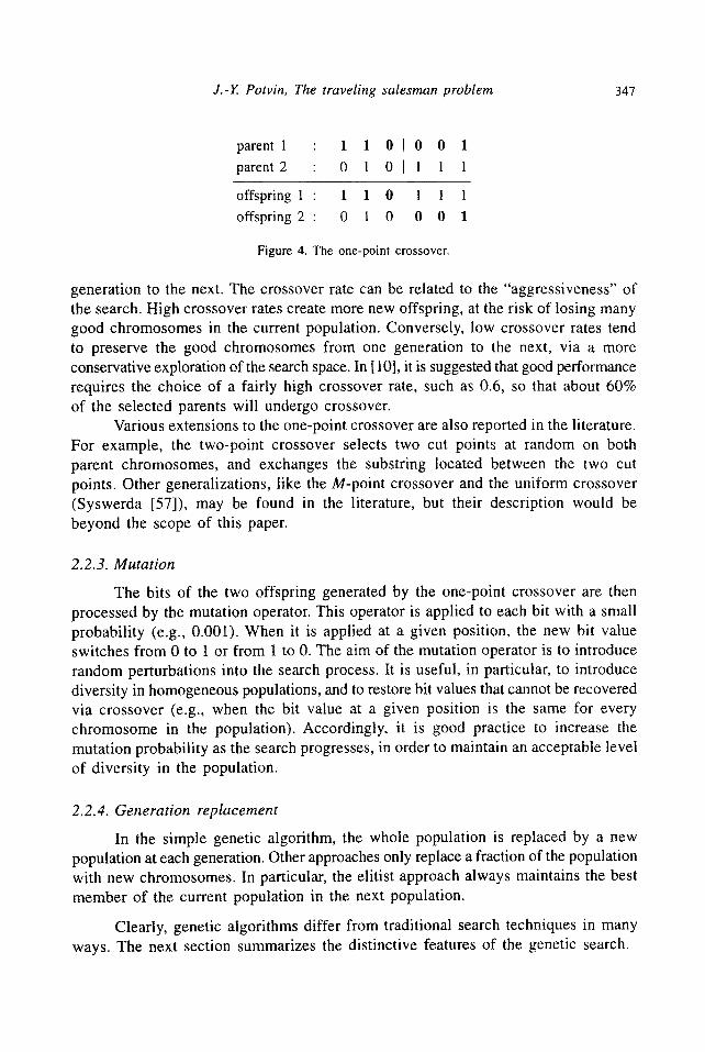
The one-point crossover operator is aimed at exchanging bit strings between two parent chromosomes. A random position between 1 and L - 1 is chosen along the two parent chromosomes, where L is the chromosome's length. Then, the chromosomes are cut at the selected position, and their end parts are exchanged to create two offspring. In figure 4, for example, the parent chromosomes are cut at position 3.

A probability is associated to the application of the crossover operator. If the operator is not applied to the selected parents, they are copied to the new population without any modification. In this way, good chromosomes can be preserved from one


parent 1 : 1 1 0 I 0 0 1 parent 2 : 0 1 0 I 1 1 1

offspring 1 : 1 1 0 1 1 1 offspring 2 : 0 1 0 0 0 1

Figure 4. The one-point crossover.

generation to the next. The crossover rate can be related to the "aggressiveness" of the search. High crossover rates create more new offspring, at the risk of losing many good chromosomes in the current population. Conversely, low crossover rates tend to preserve the good chromosomes from one generation to the next, via a more conservative exploration of the search space. In [ 10], it is suggested that good performance requires the choice of a fairly high crossover rate, such as 0.6, so that about 60% of the selected parents will undergo crossover.

Various extensions to the one-point crossover are also reported in the literature. For example, the two-point crossover selects two cut points at random on both parent chromosomes, and exchanges the substring located between the two cut points. Other generalizations, like the M-point crossover and the uniform crossover (Syswerda [57]), may be found in the literature, but their description would be beyond the scope of this paper.

2.2.3. Mutation

The bits of the two offspring generated by the one-point crossover are then processed by the mutation operator. This operator is applied to each bit with a small probability (e.g., 0.001). When it is applied at a given position, the new bit value switches from 0 to 1 or from 1 to 0. The aim of the mutation operator is to introduce random perturbations into the search process. It is useful, in particular, to introduce diversity in homogeneous populations, and to restore bit values that cannot be recovered via crossover (e.g., when the bit value at a given position is the same for every chromosome in the population). Accordingly, it is good practice to increase the mutation probability as the search progresses, in order to maintain an acceptable level of diversity in the population.

2.2.4. Generation replacement

In the simple genetic algorithm, the whole population is replaced by a new population at each generation. Other approaches only replace a fraction of the population with new chromosomes. In particular, the elitist approach always maintains the best member of the current population in the next population.

Clearly, genetic algorithms differ from traditional search techniques in many ways. The next section summarizes the distinctive features of the genetic search.

348 J.-Y Potvin, The traveling salesman problem

2.3. CHARACTERISTICS OF THE GENETIC SEARCH

Broadly speaking, the search performed by a genetic algorithm can be characterized in the following way (Goldberg [20]):

(a) Genetic algorithms manipulate bit strings or chromosomes encoding useful information about the problem, but they do not manipulate the information as such (no decoding or interpretation).

(b) Genetic algorithms use the evaluation of a chromosome, as returned by the fitness function, to guide the search. They do not use any other information about the fitness function or the application domain.

(c) The search is run in parallel from a population of chromosomes. (d) The transition from one chromosome to another in the search space is done

stochastically.

In particular, points (a) and (b) explain the robustness of the genetic algorithms and their wide applicability as meta-heuristics in various application domains. However, the simple genetic search introduced in this section cannot be directly applied to a combinatorial optimization problem like the TSP. The next section will now provide more explanations on this matter.

3. Genetic algorithms for the TSP

The description of the genetic algorithm of section 2 included many genetic terms. In order to better understand how genetic algorithms can be applied to combinatorial optimization problems, the following equivalence will be useful.

Combinatorial optimization Genetic algorithm

Encoded solution Solution Set of solutions Objective function

Chromosome Decoded chromosome Population Fitness function

In a TSP context, each chromosome encodes a solution to the problem (i.e., a tour). The fitness of the chromosome is related to the tour length, which in turn depends on the ordering of the cities. Since the TSP is a minimization problem, the tour lengths must be transformed so that high fitness values are associated with short tours, and conversely. A well-known approach is to subtract each tour length to the maximum tour length found in the current population. Other approaches are based on the rank of the tours in the population (as mentioned in the previous section).


The genetic algorithm searches the space of solutions by combining the best features of two good tours into a single one. Since the fitness is related to the length of the edges included in the tour, it is clear that the edges represent the basic information to be transferred to the offspring. The success or failure of the approaches described in the following sections can often be explained by their ability or inability to adequately represent and combine the edge information in the offspring.

Difficulties quickly arise when the simple "pure" genetic algorithm of section 2 is applied to a combinatorial optimization problem like the TSP. In particular, the encoding of a solution as a bit string is not convenient. Assuming a TSP of size N, each city would be coded using [log2N] bits, and the whole chromosome would encode a tour as a sequence o f N * [log2N] bits. Accordingly, most sequences in the search space would not correspond to feasible tours. For example, it would be easy to create a sequence with two occurrences of the same city, using the mutation operator. Moreover, when the number of cities is not a power of two, some bit sequences in the code would not correspond to any city. In the literature, fitness functions with penalty terms, and repair operators to transform infeasible solutions into feasible ones, have been proposed to alleviate these problems (Richardson et al. [52], Siedlecki and Sklanski [54], Michalewicz and Janikow [41]). However, these approaches were designed for very specific application domains, and are not always relevant in a TSP context.

The preferred research avenue for the TSP is to design representational frameworks that are more sophisticated than the bit string, and to develop specialized operators to manipulate these representations and create feasible sequences. For example, the chromosomes shown in figure 5 are based on the "path" representation of a tour (on cities 1 to 8). It is clear that the mutation operator and the one-point crossover are still likely to generate infeasible tours when they are applied to this integer representation. For example, applying the crossover operator at position 2 creates two infeasible offspring, as illustrated in figure 5.

tour (12564387) : 1 2 1 5 6 4 3 8 7 tour (14236578) : 1 4 1 2 3 6 5 7 8

offspringl : 1 2 2 3 6 5 7 8 offspring2 : 1 4 5 6 4 3 8 7

Figure 5. Application of the one-point crossover on two parent tours.

None of the two offspring is a permutation of the cities. The TSP, as opposed to most problems tackled by genetic algorithms, is a pure ordering problem. Namely, all chromosomes carry exactly the same values and differ only in the ordering of these values. Accordingly, specialized permutation operators must be developed for this problem.


In the following sections, we explain how genetic algorithms can be tailored to the TSP. The extensions proposed in the literature will be classified according to the representational framework used to encode a TSP tour into a chromosome, and the crossover operators used to manipulate these representations.

4. The ordinal representation

In [22], the authors developed an ingenious coding scheme for the classical one-point crossover. With this coding scheme, the one-point crossover always generates feasible offspring. This representation is mostly of historical interest, because the sequencing information in the two parent chromosomes is not well transferred to the offspring, and the resulting search is close to a random search.

The encoding is based on a reference or canonic tour. For N = 8 cities, let us assume that this canonic tour is 12345678. Then, the tour to be encoded is processed city by city. The position of the current city in the canonic tour is stored at the corresponding position in the resulting chromosome. The canonic tour is updated by deleting that city, and the procedure is repeated with the next city in the tour to be encoded.

This approach is illustrated in figure 6 using a small example. In this figure, the first string is the current tour to be encoded, the second string is the canonic tour and the third string is the resulting chromosome. The underlined city in the first string corresponds to the current city. The position of the current city in the canonic tour is used to build the ordinal representation.

Cu~enttour Canonictour Ordinalrepresentation ! 2 5 6 4 3 8 7 ! 2 3 4 5 6 7 8 I 1 2 5 6 4 3 8 7 2 3 4 5 6 7 8 11 1 2 5 6 4 3 8 7 3 4 5 6 7 8 1 1 3 1 2 5 6 4 3 8 7 3 4 6 7 8 1 1 3 3 1 2 5 6 4 3 8 7 3 4 7 8 1 1 3 3 2 1 2 5 6 4 3 8 7 3 7 8 1 1 3 3 2 1 1 2 5 6 4 3 8 7 7 8 1 1 3 3 2 1 2 1 2 5 6 4 3 8 Z 7 1 1 3 3 2 1 2 1

Figure 6. The ordinal representation.

The resulting chromosome 11332121 can be easily decoded into the original tour 12564387 by the inverse process. Interestingly enough, two parent chromosomes encoded in this way always generate a feasible offspring when they are processed by the one-point crossover. In fact, each value in the ordinal representation corresponds to a particular position in the canonic tour. Exchanging values between two parent


chromosomes simply modified the order of selection of the cities in the canonic tour. Consequently, a permutation is always generated. For example, the two parent chromosomes in figure 7 encode the tours 12564387 and 14236578, respectively. After a cut at position 2, a feasible offspring is created.

parent 1 (12564387) : 1 1 ] 3 3 2 1 2 1 parent 2 (14236578) : 1 3 I I 1 2 1 1 1

offspring (12346578) : 1 1 ! 1 2 1 1 1

Figure 7. Application of the one-point crossover on two parent tours using the ordinal representation,

5. The path representation

As opposed to the ordinal representation, the path representation is a natural way to encode TSP tours. However, a single tour can be represented in 2N distinct ways, because any city can be placed at position 1, and the two orientations of the tour are the same for a symmetric problem. Of course, the factor N can be removed by fixing a particular city at position 1 in the chromosome.

The crossover operators based on this representation typically generate offspring that inherit either the relative order or the absolute position of the cities from the parent chromosomes. We will now describe these operators in turn. In each case, a single offspring is shown. However, a second offspring can be easily generated by inverting the roles of the parents.

5.1. CROSSOVER OPERATORS PRESERVING THE ABSOLUTE POSITION

The two crossover operators introduced in this section were among the first to be designed for the TSP. Generally, speaking, the results achieved with these operators are not very impressive (as reported at the end of this section).

5.1.1. Partially-mapped crossover (PMX) (Goldberg and Lingle [18])

This operator first randomly selects two cut points on both parents. In order to create an offspring, the substring between the two cut points in the first parent replaces the corresponding substring in the second parent. Then, the inverse replacement is applied outside of the cut points, in order to eliminate duplicates and recover all cities.

In figure 8, the offspring is created by first replacing the substring 236 in parent 2 by the substring 564. Hence, city 5 replaces city 2, city 6 replaces city 3, and city 4 replaces city 6 (step 1). Since cities 4 and 5 are now duplicated in the offspring, the inverse replacement is applied outside of the cut points. Namely, city 2


parent 1 parent 2

1 2 1 5 6 4 1 3 8 7 1 4 I 2 3 6 I 5 7 8

offspring (step 1) (step 2)

1 4 5 6 4 5 7 8 1 3 5 6 4 2 7 8

Figure 8. The partially-mapped crossover.

replaces city 5, and city 3 replaces city 4 (step 2). In the latter case, city 6 first replaces city 4, but since city 6 is already found in the offspring at position 4, city 3 finally replaces city 6. Multiple replacements at a given position occur when a city is located between the cut points on both parents, like city 6 in this example.

Clearly, PMX tries to preserve the absolute position of the cities when they are copied from the parents to the offspring. In fact, the number of cities that do not inherit their positions from one of the two parents is at most equal to the length of the string between the two cut points. In the above example, only cities 2 and 3 do not inherit their absolute position from one of the two parents.

5.1.2. Cycle crossover (CX) (Oliver et al. [47])

The cycle crossover focuses on subsets of cities that occupy the same subset of positions in both parents. Then, these cities are copied from the first parent to the offspring (at the same positions), and the remaining positions are filled with the cities of the second parent. In this way, the position of each city is inherited from one of the two parents. However, many edges can be broken in the process, because the initial subset of cities is not necessarily located at consecutive positions in the parent tours.

In figure 9, the subset of cities { 3, 4, 6 } occupies the subset of positions { 2, 4, 5 } in both parents. Hence, an offspring is created by filling the positions 2, 4 and 5 with the cities found in parent 1, and by filling the remaining positions with the cities found in parent 2.

parent 1 : 1 3 5 6 4 2 8 7 parent 2 : 1 4 2 3 6 5 7 8

offspring : 1 3 2 6 4 5 7 8

Figure 9. The cycle crossover.

Note that the crossover operator introduced in [6] is a restricted version of CX, where the subset of cities must occupy consecutive positions in both parents.


5.1.3. Computational results

Goldberg and Lingle [18] tested the PMX operator on the small 10-city TSP in [31] and reported good results. One run generated the optimal tour of length 378, and the other run generated a tour of length 381. However, later studies (Oliver et al. [47], Starkweather et al. [55]) demonstrated that PMX and CX were not really competit ive with the order-preserving crossover operators (see section 5.2).

5.2. CROSSOVER OPERATORS PRESERVING THE RELATIVE ORDER

Most operators discussed in this section were designed a few years after the operators of section 5.2, and generally provide much better results on TSPs.

5.2.1. Modified crossover (Davis [9])

This crossover operator is an extension of the one-point crossover for permutation problems. A cut position is chosen at random on the first parent chromosome. Then, an offspring is created by appending the second parent chromosome to the initial segment of the first parent (before the cut point), and by eliminating the duplicates. An example is provided in figure 10.

parent 1 parent 2

1 2 1 5 6 4 3 8 7 1 4 2 3 6 5 7 8

offspring 1 2 4 3 6 5 7

Figure 10. The modified crossover.

Note that the cities occupying the first positions in parent 2 tend to move forward in the resulting offspring (with respect to their positions in parent 1). For example, city 4 occupies the fifth position in parent 1, but since it occupies the second position in parent 2, it moves to the third position in the resulting offspring.

5.2.2. Order crossover (OX) (Oliver et al. [47], Goldberg [20])

This crossover operator extends the modified crossover of Davis by allowing two cut points to be randomly chosen on the parent chromosomes. In order to create an offspring, the string between the two cut points in the first parent is first copied to the offspring. Then, the remaining positions are filled by considering the sequence of cities in the second parent, starting after the second cut point (when the end of the chromosome is reached, the sequence continues at position 1).

In figure 11, the substring 564 in parent 1 is first copied to the offspring (step 1). Then, the remaining positions are filled one by one after the second cut point,


parent 1 : 1 2 I 5 6 4 1 3 8 7 parent 2 : 1 4 I 2 3 6 I 5 7 8

offspring (step 1) : 5 6 4 (step 2) : 2 3 5 6 4 7 8 1

Figure 11. The order crossover.

by considering the corresponding sequence of cities in parent 2, namely 57814236 (step 2). Hence, city 5 is first considered to occupy position 6, but it is discarded because it is already included in the offspring. City 7 is the next city to be considered, and it is inserted at position 6. Then, city 8 is inserted at position 7, city 1 is inserted at position 8, city 4 is discarded, city 2 is inserted at position 1, city 3 is inserted at position 2, and city 6 is discarded.

Clearly, OX tries to preserve the relative order of the cities in parent 2, rather than their absolute position. In figure 11, the offspring does not preserve the position of any city in parent 2. However, city 7 still appears before city 8 and city 2 before city 3 in the resulting offspring. It is worth noting that a variant of OX, known as the maximal preservative crossover, is also described in [21].

5.2.3. Order-based crossover (OBX) (Syswerda [58])

This crossover also focuses on the relative order of the cities on the parent chromosomes. First, a subset of cities is selected in the first parent. In the offspring, these cities appear in the same order as in the first parent, but at positions taken from the second parent. Then, the remaining positions are filled with the cities of the second parent.

In figure 12, cities 5, 4 and 3 are first selected in parent I, and must appear in this order in the offspring. Actually, these cities occupy positions 2, 4 and 6 in parent 2. Hence, cities 5, 4 and 3 occupy positions 2, 4 and 6, respectively, in the offspring. The remaining positions are filled with the cities found in parent 2.

parent 1 : 1 2 _5 6 4 3 8 7 parent 2 : 1 4 2 3 6 5 7 8

offspring : 1 5 2 4 6 3 7 8

Figure 12. The order-based crossover.

5.2.4. Position-based crossover (PBX) (Syswerda [58])

Here, a subset of positions is selected in the first parent. Then, the cities found at these positions are copied to the offspring (at the same positions). The other positions are filled with the remaining cities, in the same order as in the second parent.


The name of this operator is a little bit misleading, because it is the relative order of the cities that is inherited from the parents (the absolute position of the cities inherited from the second parent is rarely preserved). This operator can be seen as an extension of the order crossover OX, where the cities inherited from the first parent do not necessarily occupy consecutive positions.

In figure 13, positions 3, 5 and 6 are first selected in parent 1. Cities 5, 4 and 3 are found at these positions, and occupy the same positions in the offspring. The other positions are filled one by one, starting at position 1, by inserting the remaining cities according to their relative order in parent 2, namely 12678.

parent 1 : 1 2 _5 6 4 3 8 7 parent 2 : 1 4 2 3 6 5 7 8

offspring : 1 2 5 6 4 3 7 8

Figure 13. The position-based crossover.

5.2.5. Computational results

Studies by Oliver et al. [47] and Starkweather et al. [55] demonstrated that order-preserving crossover operators were clearly superior to the operators preserving the absolute position of the cities.

In [47], PMX, CX and OX were applied to the 30-city problem of Hopfield and Tank [28]. They found that the best tour generated with OX was 11% shorter than the best PMX tour, and 15% shorter than the best CX tour. In a later study [55], six different crossover operators were tested on the same problem [28]. Thirty different runs were performed with each operator. In this experiment, OX found the optimum 25 times (out of 30), while PMX found the optimum only once, and CX never found the optimum.

Table 1

Comparison of six crossover operators (30 runs) in [55].

Crossover No. of trials Pop. size Optimum Ave. tour length

Edge recombination (ER) 30,000 1,000 30/30 420.0 Order (OX) 100,000 1,000 25/30 420.7 Order based (OBX) 100,000 1,000 18/30 421.4 Position based (PBX) 120,000 1,000 18/30 423.4 Partially mapped (PMX) 120,000 1,400 1/30 452.8 Cycle (CX) 140,000 1,500 0/30 490.3

Table 1 summarizes the results in [55]. It is worth noting that the parameters of the genetic algorithm were tuned for each crossover operator, so as to provide the


best possible results. Accordingly, the population size and number of trials (i.e., total number of tours generated) are not the same in each case. The edge recombination operator ER will be introduced in the next section, and should be ignored for now.

6. The adjacency representation

The adjacency representation is designed to facilitate the manipulation of edges. The crossover operators based on this representation generate offspring that inherit most of their edges from the parent chromosomes.

The adjacency representation can be described as follows: city j occupies position i in the chromosome if there is an edge from city i to city j in the tour. For example, the chromosome 38526417 encodes the tour 13564287. City 3 occupies position 1 in the chromosome because edge (1, 3) is in the tour. Similarly, city 8 occupies position 2 because edge (2, 8) is in the tour, etc. As opposed to the path representation, a tour has only two different adjacency representations for symmetric TSPs.

Various crossover operators are designed to manipulate this representation, and are introduced in the next sections. These operators are aimed at transferring as many edges as possible from the parents to the offspring. However, it is important to note that they share a common weakness: the selection of the last edge, that connects the final city to the initial city, is not enforced. In other words, the last edge is added to the final solution, without any reference to the parents. Accordingly, this edge is rarely inherited.

6.1. ALTERNATE EDGES CROSSOVER (Grefenste t te et al. [22])

This operator is mainly of historical interest. As reported in [22], the results with the operator have been uniformly discouraging. However, it is a good introduction to the other edge-preserving operators.

Here, a starting edge (i , j) is selected at random in one parent. Then, the tour is extended by selecting the edge (j , k) in the other parent. The tour is progressively extended in this way by alternatively selecting edges from the two parents. When an edge introduces a cycle, the new edge is selected at random (and is not inherited from the parents).

parent 1 : 3 8 5 2 6 4 1 7 parent 2 : 4 3 6 2 7 5 8 1

offspring : 4 3 5 2 7 8 6 1

Figure 14. The alternate edges crossover.

In figure 14, an offspring is generated from two parent chromosomes that encode the tours 13564287 and 14236578, respectively, using the adjacency


representation. Here, edge (1, 4) is first selected in parent 2, and city 4 in position I of parent 2 is copied at the same position in the offspring.

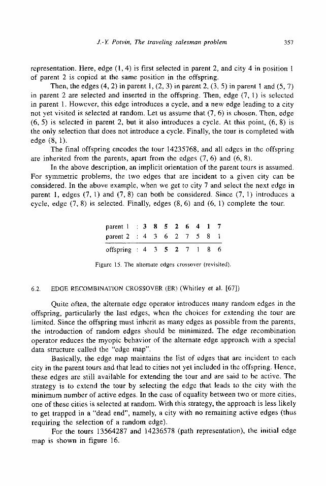
Then, the edges (4, 2) in parent 1, (2, 3) in parent 2, (3, 5) in parent 1 and (5, 7) in parent 2 are selected and inserted in the offspring. Then, edge (7, 1) is selected in parent 1. However, this edge introduces a cycle, and a new edge leading to a city not yet visited is selected at random. Let us assume that (7, 6) is chosen. Then, edge (6, 5) is selected in parent 2, but it also introduces a cycle. At this point, (6, 8) is the only selection that does not introduce a cycle. Finally, the tour is completed with edge (8, 1).

The final offspring encodes the tour 14235768, and all edges in the offspring are inherited from the parents, apart from the edges (7, 6) and (6, 8).

In the above description, an implicit orientation of the parent tours is assumed. For symmetric problems, the two edges that are incident to a given city can be considered. In the above example, when we get to city 7 and select the next edge in parent 1, edges (7, 1) and (7, 8) can both be considered. Since (7, 1) introduces a cycle, edge (7, 8) is selected. Finally, edges (8, 6) and (6, 1) complete the tour.

parent 1 : 3 8 5 2 6 4 1 7 parent 2 : 4 3 6 2 7 5 8 1

offspring : 4 3 5 2 7 I 8 6

Figure 15. The alternate edges crossover (revisited).

6.2. EDGE RECOMBINATION CROSSOVER (ER) (Whitley et al. [67])

Quite often, the alternate edge operator introduces many random edges in the offspring, particularly the last edges, when the choices for extending the tour are limited. Since the offspring must inherit as many edges as possible from the parents, the introduction of random edges should be minimized. The edge recombination operator reduces the myopic behavior of the alternate edge approach with a special data structure called the "edge map".

Basically, the edge map maintains the list of edges that are incident to each city in the parent tours and that lead to cities not yet included in the offspring. Hence, these edges are still available for extending the tour and are said to be active. The strategy is to extend the tour by selecting the edge that leads to the city with the min imum number of active edges. In the case of equality between two or more cities, one of these cities is selected at random. With this strategy, the approach is less likely to get trapped in a "dead end", namely, a city with no remaining active edges (thus requiring the selection of a random edge).

For the tours 13564287 and 14236578 (path representation), the initial edge map is shown in figure 16.


c~ty city city c~ty city city c~ty city

1 has edges to : 3 4 7 2 has edges to : 3 4 8 3 has edges to : 1 2 5 4 has edges to : 1 2 6 5 has edges to : 3 6 7 6 has edges to : 3 4 5 7 has edges to : 1 5 8 8 has edges to : 1 2 7

Figure 16. The edge map.

(a) City I is selected

city 2 has edges to : 3 4 8 city 3 has edges to : 2 5 6 city 4 has edges to : 2 6 city 5 has edges to : 3 6 7 city 6 has edges to : 3 4 5 city 7 has edges to : 5 8 city _8 has edges to : 2 7

(b) City 8 is selected

city 2 has edges to : 3 4 city 3 has edges to : 2 5 6 city 4 has edges to : 2 6 city 5 has edges to : 3 6 7 city 6 has edges to : 3 4 5 city 7 has edges to : 5

(c) City 7 is selected

city 2 has edges to : 3 4 city 3 has edges to : 2 5 6 city 4 has edges to : 2 6 city 5 has edges to : 3 6 city 6 has edges to : 3 4 5

(d)

City 5 is selected

city 2 has edges to : 3 4 city 3 has edges to : 2 6 city 4 has edges to : 2 6 city 6 has edges to : 3 4

(e) City 6 is selected

city 2 has edges to : 3 4 city 3 has edges to : 2 city 4 has edges to : 2

(f) City 4 is selected

city 2 has edges to : 3 city 3 has edges to : 2 6

(g) City 2 is selected City 3 is selected

city 3 has edges to :

Figure 17. Evolution of the edge map.

T h e opera t ion o f the edge r ecombina t i on c r o s s o v e r ope ra to r will n o w be i l lustrated on this ini t ia l e d g e m a p (see f igu re 17). To this end , the e d g e m a p wil l be u p d a t e d a f t e r e ach c i ty se lec t ion . In these e d g e m a p s , c i t ies o f pa r t i cu l a r in te res t are u n d e r l i n e d ( n a m e l y , c i t ies tha t are a d j a c e n t to the s e l ec t ed c i ty in the pa r en t s and are not v i s i t ed ye t ) .


Let us assume that city 1 is selected as the starting city. Accordingly, all edges incident to city 1 must first be deleted from the initial edge map. From city 1, we can go to cities 3, 4, 7 or 8. City 3 has three active edges, while cities 4, 7 and 8 have two active edges, as shown by edge map (a) in figure 17. Hence, a random choice is made between cities 4, 7 and 8. We assume that city 8 is selected. From 8, we can go to cities 2 and 7. As indicated in edge map (b), city 2 has two active edges and city 7 only one, so the latter is selected. From city 7, there is no choice but to go to city 5. From this point, edge map (d) offers a choice between cities 3 and 6 with two active edges. Let us assume that city 6 is randomly selected. From city 6, we can go to cities 3 and 4, and edge map (e) indicates that both cities have one active edge. We assume that city 4 is randomly selected. Finally, from city 4 we can only go to city 2, and from city 2 we must go to city 3. The final tour is 18756423 and all edges are inherited from both parents.

A variant which focuses on edges common to both parents is also described in [55]. The common edges are marked with an asterisk in the edge map, and are always selected first (even if they do not lead to the city with the minimum number of active edges). In the previous example, (2, 4), (5, 6) and (7, 8) are found in both parents and have priority over all other active edges. In the above example, the new approach generates the same tour, because the common edges always lead to the cities with the minimum number of active edges.

6.3. HEURISTIC CROSSOVER (HX) [Grefenstette et al. [22], Grefenstette [23])

It is worth noting that the previous crossover operators did not exploit the distances between the cities (i.e., the length of the edges). In fact, it is a characteristic of the genetic approach to avoid any heuristic information about a specific application domain, apart from the overall evaluation or fitness of each chromosome. This characteristic explains the robustness of the genetic search and its wide applicability.

However, some researchers departed from this line of thinking and introduced domain-dependent heuristics into the genetic search to create "hybrid" genetic algorithms. They have sacrificed robustness over a wide class of problems for better performance on a specific problem. The heuristic crossover HX is an example of this approach and can be described as follows:

Step 1. Step 2.

Step 3.

Step 4.

Choose a random starting city from one of the two parents.

Compare the edges leaving the current city in both parents and select the shorter edge.

If the shorter parental edge introduces a cycle in the partial tour, then extend the tour with a random edge that does not introduce a cycle.

Repeat steps 2 and 3 until all cities are included in the tour.


Note that a variant is proposed in [36,56] to emphasize the inheritance of edges from the parents. Basically, step 3 is modified as follows:

Step 3'. If the shorter parental edge introduces a cycle, then try the other parental edge. If it also introduces a cycle, then extend the tour with a random edge that does not introduce a cycle.

Jog et al. [29] also proposed to replace the random edge selection by the selection of the shortest edge in a pool of random edges (the size of the pool being a parameter of the algorithm).

6.4. COMPUTATIONAL RESULTS

Results reported in the literature show that the edge-preserving operators are superior to the other types of crossover operators (Liepins et al. [37], Starkweather et al. [55]). In particular, the edge recombination ER outperformed all other tested operators in the study of Starkweather et al. [55]. A genetic algorithm based on ER was run 30 times on the 30-city problem described in [28], and the optimal tour was found on each run (see table 1).

However, these operators alone cannot routinely find good solutions to larger TSPs. For example, Grefenstette et al. [22] applied the heuristic crossover HX to three TSPs of size 50, 100 and 200, and the reported solutions were as far as 25%, 16% and 27% over the optimum, respectively. Generally speaking, many edge crossings can still be observed in the solutions generated by the edge-preserving operators. Accordingly, powerful mutation operators based on k-opt exchanges (Lin [38]) are added to these operators to improve solution quality. These hybrid schemes will be discussed in the next section.

Table 2 summarizes sections 4 to 6 by providing a global view of the various crossover operators for the TSP. They are classified according to the type of information transferred to the offspring (i.e., relative order of the cities, absolute position of the cities, or edges).

Table 2

Information inheritance for nine crossover operators.

Crossover operator Relative order Position Edge

Modified Order (OX) Order based (OBX) Position based (PBX) Partially mapped (PMX) Cycle (CX) Alternate edge Edge recombination (ER) Heuristic (HX)

X

X

X

X

X

X

X


As a final remark, it is worth noting that Fox and McMahon [13] describe an alternative matrix-based encoding of the TSP tours. Boolean matrices, encoding the predecessor and successor relationships in the tour, are manipulated by special union and intersection crossover operators. This approach provided mixed results on problems with four different topologies. In particular, union and intersection operators were both outperformed by simple unary mutation operators. However, these operators presented an interesting characteristic: they managed to make progress even when elitism was not used (i.e., when the best tour in a given population was not preserved in the next population).

Recently, Homaifar et al. [27] reported good results with another matrix-based encoding of the tours. In this work, each chromosome corresponds to the adjacency matrix of a tour (i.e., the entry (i , j) in the matrix is 1 if arc (i,j) is in the tour). Accordingly, there is exactly one entry equal to 1 in each row and column of the matrix. Then, the parent chromosomes produce offspring by exchanging columns via a specialized matrix-based crossover operator called MX. Since the resulting offspring can have rows with either no entry or many entries equal to 1, a final "repair." operator is applied to generate valid adjacency matrices. A 2-opt exchange heuristic is also used to locally optimize the solutions. With this approach, the authors solved eight classical TSP problems ranging in size from 25 to 318 nodes, and they matched the best known solutions for five problems out of eight.

7. Mutation operators

Mutation operators for the TSP are aimed at randomly generating new permutations of the cities. As opposed to the classical mutation operator, which introduces small perturbations into the chromosome, the permutation operators for the TSP often greatly modifies the original tour. These operators are summarized below.

7.1. SWAP

Two cities are randomly selected and swapped (i.e., their positions are exchanged). This mutation operator is the closest in philosophy to the original mutation operator, because it only slightly modifies the original tour.

7.2. LOCAL HILL-CLIMBING

Typically, a local edge exchange heuristic is applied to the tour (e.g., 2-opt, 3-opt). The exchange heuristic is applied for a fixed number of iterations, or until a local optimum is found. Note that the reordering operator known as inversion (Holland [26]) corresponds to a single 2-opt exchange.

362 J.-Y. Port, in, The traveling salesman problem

7.3. SCRAMBLE

Two cut points are selected at random on the chromosome, and the cities within the two cut points are randomly permuted.


The studies of Suh and Gucht [56], Jog et al. [29], and Ulder et al. [64] pointed out the importance of the hill-climbing mutation operators. Suh and Gucht added a 2-opt hill-climbing mutation operator to the heuristic crossover HX. On the first 100- city problem in [33], they found a tour of length 21,651, only 1.7% over the optimum. The heuristic crossover HX alone found a solution as far as 25% over the optimum.

On the same problem, Jog et al. [29] found that the average and best tours, over 10 different runs, were 2.6% and 0.8% over the optimum using a similar approach based on HX and 2-opt. By adding Or-opt (i.e., some chromosomes perform a 2-opt hill-climbing, while others perform an Or-opt), the average and best solutions improved to 1.4% and 0.01% over the optimum, respectively.

In [64], eight classical TSPs ranging in size from 48 to 666 cities were solved with a genetic algorithm based on the order crossover OX and the Lin-Kernighan hill-climbing heuristic. Five runs were performed on each problem and the averages were within 0.4% of the optimum in each case. Table 3 shows their results for the three largest problems of size 442, 532 and 666 (Padberg and Rinaldi [49], Gr6tschel and Holland [24]). This genetic algorithm was compared with four other solution

Table 3

Average percent over the optimum (5 runs) for five solution procedures in [64].

CPU time SA M - 2 o p t M - L K G-2op t G-LK TSP (seconds) (%) (%) (%) (%) (%)

442-city 4,100 2.60 9.29 0.27 3.02 0.19 532-city 8,600 2.77 8.34 0.37 2.99 0.17 666-city 17,000 2.19 8.67 1.18 3.45 0.36

SA simulated annealing. M-2opt Multi-start 2-opt (a new starting point is chosen when a local optimum is

found). M-LK Multi-start Lin-Kernighan. G-2opt Genetic algorithm with 2-opt mutation operator. G-LK Genetic algorithm with Lin-Kernighan mutation operator.

procedures, and it found the best solution in each case. All approaches were allowed the same amount of computation time on a VAX 8650, using the computation time of the simulated annealing heuristic as the reference. In table 3, the number in each cell is the average percent over the optimum.


Braun [7] also reported interesting results on the 442- and 666-city problems. Fifty different runs were performed with a genetic algorithm based on the order crossover OX and a mixed 2-opt, Or-opt hill-climbing. He found the optimum of the 442-city problem, and a solution within 0.04% of the optimum for the 666-city problem. On a 431-city problem, each run generated a solution within 0.5% of the optimum, and about 25% of the solutions were optimal. In the latter case, the average run time on a Sun workstation was about 30 minutes. Braun also reported that a 229- city problem was solved in less than three minutes.

8. Parallel implementations

The genetic algorithm is well suited for parallel implementations, because it is applied to a population of solutions. In particular, a parallel implementation described in [21,43-45] was very successful on some large TSPs.

In this implementation, each processor handles a single chromosome. Since the processors (chromosomes) are linked together according to a fixed topology, the population of chromosomes is structured. Namely, a neighborhood can be established around each chromosome based on this topology, and reproduction takes place among neighboring chromosomes only. Since the neighborhoods intersect, the new genetic material slowly "diffuses" through the whole population. One main benefit of this organization over a uniform population, where each chromosome can mate with any other chromosome, is that diversity is more easily maintained in the population. Accordingly, the parallel genetic algorithm can work with smaller populations without suffering from premature convergence.

The parallel genetic algorithm can be described as follows.

Step 1. Step 2.

Step 3. Step 4.

Step 5.

Create an initial random population.

Each chromosome performs a local hill-climbing (2-opt).

Each chromosome selects a partner for mating in its neighborhood.

An offspring is created with an appropriate crossover operator (OX).

The offspring performs a local hill-climbing (2-opt). Then, it replaces its parent if the two conditions below are satisfied: (a) it is better than the worst chromosome in the parent's neighborhood; (b) it is better than the parent, if the parent is the best chromosome in its

neighborhood (elitist strategy).

This algorithm is totally asynchronous. Each chromosome selects a partner for mating in its neighborhood without any regard for the population as a whole (which implies that some chromosomes can be at generation T, while other chromosomes are at generation T + 1 or more). Note also that the algorithm always searches for new


local optima. In particular, it combines two local optima to generate a new local optimum that is hopefully better than the two previous ones.

In [68], the authors describe an alternative implementation where subpopulations of chromosomes evolve in parallel on different processors. After a fixed number of iterations (based on the size of the subpopulations), the best chromosomes on each processor migrate to a neighboring processor and replace the worst chromosomes on that processor. A similar idea is also found in [7].


Whitley et al. [68] solved a 105-city problem with their distributed approach based on migration using the edge recombination operator ER for crossover and no mutation operator. With this parallel algorithm, they found the optimum tour in 15 different runs (out of 30). In addition, 29 solutions were within 0.5% of the optimum, and all solutions were within 1% of the optimum.

The parallel genetic algorithm [21,44] was applied to the classical 442- and 532-city problems described in [24,49]. On a parallel computer with 64 T800 transputers, this algorithm solved the two problems in approximately 0.6 and one hour, respectively (the computation times can change depending on the parameter settings). The best solutions for the 442- and 666-city problems were within 0.3% and 0.1% of the optimum, respectively. Note that Braun [7] found the optimal solution of the 442-city problem with his approach (cf. section 7).

9. Overview of the computational results

The results published in the literature on genetic algorithms cannot be easily compared, because various algorithmic designs and parameter settings are used. With respect to the algorithmic design, most implementations use a proportional selection scheme based on some transformation of the raw fitness value or tour length (cf. scaling, ranking, etc.). Various generation replacement mechanisms are also described, ranging from a complete replacement of the population without any form of elitism, to the replacement of the worst tour by a single newly created tour. Judicious parameter settings can also improve the quality of the final solution (e.g., population size, maximum number of generations, crossover and mutation rates, etc.). Finally, the initial population can be generated in various ways (e.g., random tours versus heuristic tours).

Although a particular implementation scheme can influence the quality of the final solution, we avoided implementation details in the previous sections to focus on the crossover and mutation operators only. This approximation greatly simplified the description of the computational results. Generally speaking, the results published in the literature support the following conclusions:


(a) The edge-preserving crossover operators outperform the operators that preserve the relative order or the absolute position of the cities.

(b) The combination of crossover and local hill-climbing mutation is critical to the success of the genetic algorithm. Crossover alone typically generates tours with many edge crossings (which can be easily eliminated with a 2-opt).

(c) An efficient approach for solving large TSPs is to divide the population of chromosomes into subpopulations. The subpopulations evolve in parallel and periodically exchange genetic material. This approach alleviates premature convergence by maintaining an acceptable level of diversity. Hence, large problems can be solved with relatively small populations.

(d) For any given implementation, the quality of the final solution increases with the size of the population. This result is also related to the diversity found in large populations.

Table 4 summarizes the paper by collecting all the results presented in the previous sections. When the tour length is reported as a percentage above the best known solution, the corresponding entry is shown as +n%. For example, the best result reported in [29] on a 100-city problem is 0.01% over the best known solution. Accordingly, the entry under the column heading "Length of tour from genetic algorithm" is +0.01%.

Finally, it is worth noting that a tour of length 27,702 was found by Mulhenbein on the 532-city of Padberg and Rinaldi using the parallel genetic algorithm PGA, as reported in [30]. This solution was obtained after less than 3 hours on a network of 64 transputers. The true optimum of 27,686 was found for the first time with an exact branch-and-cut algorithm after 5 hours of computation on a supercomputer (Padberg and Rinaldi [49,50]). On the same problem, Fiechter [11] reports a tour of length 27,839 after 100 runs of the tabu search, while Johnson [30] reports a solution value of 27,705 after 20,000 different runs of the Lin-Kernighan heuristic. In the latter case, it took 530 hours on a Sequent computer to obtain this result. Finally, the iterated Lin-Kernighan heuristic, which introduces some randomization into the original exchange procedure, found the optimum on 6 runs out of 20, with an average solution value of 27,699. Each run took about 8 hours on a Sequent computer. The iterated Lin-Kernighan heuristic also found the optimum for many classical problems reported in the literature, including a problem with 2,392 cities [30].

Overall, the results reported in this section indicate that genetic algorithms are competitive with the best known heuristics for the TSP (apart from the iterated L in - Kernighan heuristic) for medium-sized TSPs with a few hundred cities. However, they require large running times to achieve good results, and they cannot be successfully applied to problems as large as those reported in the operations research literature (cf. the 1,000,000-city problems in [3]). On the other hand, genetic algorithms provide


Table 4

Main results with genetic algorithms.

Reference

Method Largest Length of Other Length of Best (crossover TSP tour from TSP tour from known

and (number genetic heuristic TSP solution mutation) of cities) algorithm heuristic

Goldberg and Lingle [18]

Grefenstette et al. [22]

Oliver et al. [47]

Liepins et al. [36]

Suh and Gucht [56]

Jog et al. [29]

Whitley et al. [68]

Gorges-Schleuter [21 ]

Braun [71

Ulder et al. [64]

Homaifar et al. [27]

PMX 10 378

HX 200 203.5

OX 30 425 a

HX 15 17,509.6 a

HX 100 21,651 and 2-opt

HX I00 + 0.01% c and 2-opt,

Or-opt

ER 105 14,383 d (parallel)

PGA 442 5,086 c[~ 532 27,715 c~'

OX 431 + 0.0% ea and 2-opt, 442 + 0.0% e

Or-opt 666 + 0.4% e

OX 442 + 0.19% rc and LK 532 + 0.17% f¢

666 + 0.36% fq

MX 318 42,154 and 2-opt

NA NA 378

NA NA t 60.2*

LK 424 424

NN 17,858.0 a'b NA

NA NA 21,282

NA NA 21,282

NA NA

NA NA

NA NA

M-LK + 0.27% rE + 0.37% f¢ + 1.18% fq

NA NA

14,383

5,069 27,694"*

171,414 5,069

294,358

5,069 27,686

294,358

41,345

a Average over 20 problems. b Best of 15 runs. c Best of 10 runs. d Best of 30 runs. e Best of 50 runs. f Average of 5 runs.

a CPU time: 15 minutes, Apollo DN4000. I~ CPU time: 0.6 hour, 64 T800 transputers.

CPU time: 1.0 hour, 64 T800 transputers. CPU time: 0.5 hour, Sun workstation. CPU time: 1.1 hours, VAX 8650.

¢ CPU time: 2.4 hours, VAX 8650. * Estimated optimum, n CPU time: 4.8 hours, VAX 8650. "*Optimal value with the misprint in the coordinates of the 265th city in [49].

LK Lin-Kernighan. NN Nearest neighbor. M-LK Multi-start Lin-Kernighan. PGA Parallel genetic algorithm. NA Not available/not applicable.

a na tu ra l f r a m e w o r k for para l le l i m p l e m e n t a t i o n s , s ince they work on a p o p u l a t i o n of so lu t ions . A c c o r d i n g l y , they wi l l grea t ly bene f i t in the fu ture f rom the spe c t a c u l a r d e v e l o p m e n t s that are t ak ing p lace in para l le l c o m p u t i n g .


10. Concluding remarks

We would like to conclude this work by mentioning some applications of genetic algorithms in other transportation-related domains. In [46], the authors describe a genetic algori thm for solving the traveling salesman problem with time windows (TSPTW). In this work, a sophisticated crossover operator is developed to handle the time window constraints. Since the operator does not guarantee feasibility, a penalty is added to the tour length when a time window is not satisfied, in order to favor feasible solutions. The authors report good results on a standard set of TSPTW problems. Blanton and Wainwright [4] also developed specialized crossover operators for multiple-vehicle routing problems with time windows and capacity constraints.

In [59-63] , a genetic algorithm is used to group customers within a "cluster first, route second" problem-solving strategy. The clustering algorithm was then applied to many different types of vehicle routing problems with various side constraints.

Applications of genetic algorithms to the linear and nonlinear transportation problems are reported in [41,42,65]. The authors use the special structure of the problem to develop sophisticated crossover and mutation operators for a matrix- based encoding of the chromosomes. These operators are designed to maintain solution feasibility during the search.

Finally, an application for the routing and scheduling of trains is described in [14].

References

[1] EH.L. Aarts, J.H.M. Korst and RJ.M. van Laarhoven, A quantitative analysis of the simulated annealing algorithm: A case study for the traveling salesman problem, J. Statist. Phys. 50(1988) 189 - 206.

[2] J.D. Bagley, The behavior of adaptive systems which employ genetic and correlation algorithms, Doctoral Dissertation, University of Michigan, Dissertation Abstracts International 28(12), 5106B (1967).

[3] J. Bentley, Fast algorithms for geometric salesman problems, ORSA J. Comp. 4(1992)387-411. [4] J.L. Blanton and R.L. Wainwright, Multiple vehicle routing with time and capacity constraints

using genetic algorithms, in: Proc. 5th Int. Conf. on Genetic Algorithms (ICGA '93), University of Illinois at Urbana-Champaign, Champaign, IL (1993) pp. 452-459.

[5l L. Bodin, B.L. Golden, A. Assad and M. Ball, Routing and scheduling of vehicles and crews: The state of the art, Comp. Oper. Res. 10(1983)63-211.

[6] R.M. Brady, Optimization strategies gleaned from biological evolution, Nature 317(1985) 804 - 806.

[7] H. Braun, On solving travelling salesman problems by genetic algorithms, in: Parallel Problem- Solving from Nature, ed. H.R Schwefel and R. Manner, Lecture Notes in Computer Science 496 (Springer) pp. 129-133.

[8] V. Cerny, Thermodynamical approach to the traveling salesman problem: An efficient simulation algorithm, J. Optim. Theory Appl. 45(1985)41-55.

[9] L. Davis, Applying adaptive algorithms to epistactic domains, in: Proc. Int. Joint Conf. on Artificial Intelligence (IJCAI '85), Los Angeles, CA (1985) pp. 162-164.

[10] K.A. De Jong, An analysis of the behavior of a class of genetic adaptive systems, Doctoral Dissertation, University of Michigan, Dissertation Abstracts International 36(10), 5140B (1975).


[11] C.N. Fiechter, A parallel tabu search algorithm for large scale traveling salesman problems, Working paper 90/1, Department of Mathematics, Ecole Polytechnique F6d~rale de Lausanne, Switzerland (1990).

[12] L.J. Fogel, A.J. Owens and M.J. Walsh, Artificial Intelligence through Simulated Evolution (Wiley, 1966)..

[13] B.R. Fox and M.B. McMahon, Genetic operators for sequencing problems, in: Foundations of Genetic Algorithms, ed. J.E. Rawlins (Morgan Kaufmann, 1991) pp. 284-300.

[14] P.S. Gabbert, D.E. Brown, C.L. Huntley, B.E Markowitz and D.E. Sappington, A system for learning routes and schedules with genetic algorithms, in: Proc. 4th Int. Conf. on Genetic Algoritl, ms (ICGA '9I), University of California at San Diego, San Diego, CA (1991) pp. 430-436.

[15] M. Gendreau, A. Hertz and G. Laporte, New insertion and post-optimization procedures for the traveling salesman problem, Oper. Res. 40(1992)1086-1094.

[16] E Glover, Tabu search, Part I, ORSA J. Comp. 1(1989)190-206. [17] E Glover, Tabu Search, Part II, ORSA J. Comp. 2(1990)4-32. [18] D.E. Goldberg and R. Lingle, Alleles, loci and the traveling salesman problem, in: Proc. 1st Int.

Conf. on Genetic Algorithms (1CGA '85), Carnegie-Mellon University, Pittsburg, PA (1985) pp. 154-159.

[19] B.L. Golden and W.R. Stewart, Empirical analysis of heuristics, in: The Traveling Salesman Problem. A Guided Tour of Combinatorial Optimization, ed. E.L. Lawler, J.K. Lenstra, A.H.G. Rinnooy Kan and D.B. Shmoys (Wiley, 1985).

[20] D.E. Goldberg, Genetic Algorithms in Search, Optimization and Machine Learning (Addison- Wesley, 1989).

[21] M. Gorges-Schleuter, ASPARAGOS: An asynchronous parallel genetic optimization strategy, in: Proc. 3rd Int. Conf. on Genetic Algorithms (ICGA '89), George Mason University, Fairfax, VA (1989) pp. 422-427.

[22] J. Grefenstette, R. Gopal, B.J. Rosmaita and D.V. Gucht, Genetic algorithms for the traveling salesman problem, in: Proc. 1st. Int. Conf. on Genetic Algorithms (ICGA '85), Carnegie-Mellon University, Pittsburgh, PA (1985) pp. 160-168.

[23] J. Grefenstette, Incorporating problem specific knowledge into genetic algorithms, in: Genetic Algorithms and Simulated Annealing, ed. L. Davis (Morgan Kaufmann, 1987) pp. 42-60.

[24] M. Gr6tschel and O. Holland, Solution of large-scale symmetric traveling salesman problems, Report 73, Institut ftir Mathematik, Universit~t Augsburg (1988).

[25] M. Held and R.M. Karp, The traveling salesman problem and minimum spanning trees, Oper. Res. 18(1970)1138-1162.

[26] J.H. Holland, Adaptation in Natural and Artificial Systems (The University of Michigan Press, Ann Arbor, 1975); reprinted by MIT Press, 1992.

[27] A. Homaifar, S. Guan and G. Liepins, A new approach to the traveling salesman problem by genetic algorithms, in: Proc. 5th Int. Conf on Genetic Algorithms (1CGA '93), University of Illinois at Urbana-Champaign, Champaign, IL (1993) pp. 460-466.

[28] J.J. Hopfield and D.W. Tank, Neural computation of decisions in optimization problems, Biol. Cybern. 52(1985)141- 152.

[29] E Jog, J.Y. Suh and D.V. Gucht, The effects of population size, heuristic crossover and local improvement on a genetic algorithm for the traveling salesman problem, in: Proc. 3rd Int. Conf on Genetic Algorithms (ICGA '89), George Mason University, Fairfax, VA (1989) pp. 110-115.

[30] D.S. Johnson, Local optimization and the traveling salesman problem, in: Automata, Languages and Programming, ed. G. Goos and J. Hartmanis, Lecture Notes in Computer Science 443 (Springer, 1990) pp. 446- 461.

[31] R.L. Karg and G.L. Thompson, A heuristic approach to solving traveling salesman problems, Manag. Sci. 10(1964)225-248.

[32] S. Kirkpatrick, C.D. Gelatt and M.P. Vecchi, Optimization by simulated annealing, Science 220( 1983)671 - 680.


[33] P.D. Krolak, W. Felts and G. Marble, A man-machine approach toward solving the traveling salesman problem, Commun. ACM 14(1971)327-334.

[34] G. Laporte, The traveling salesman problem: An overview of exact and approximate algorithms, Euro. J. Oper. Res. 59(1992)231-247.

[35] E.L. Lawler, J.K. Lenstra, A.H.G. Rinnooy Kan and D.B. Shmoys, The Traveling Salesman Problem: A Guided Tour of Combinatorial Optimization (Wiley, 1985).

[36] G.E. Liepins, M.R. Hilliard, M. Palmer and M. Morrow, Greedy genetics, in: Proc. 2nd Int. Conf. on Genetic Algorithms (ICGA '87), Massachusetts Institute of Technology, Cambridge, MA (1987) pp. 90-99.

[37] G.E. Liepins, M.R. Hilliard, J. Richardson and M. Palmer, Genetic algorithm applications to set covering and traveling salesman problems, in: Operations Research and Artificial Intelligence: The Integration of Problem Solving Strategies, ed. Brown and White (Kluwer Academic, 1990) pp. 29-57.

[38] S. Lin, Computer solutions of the traveling salesman problem, Bell Syst. Tech. J. 44(1965) 2245 -2269.

[39] S. Lin and B. Kernighan, An effective heuristic algorithm for the traveling salesman problem, Oper. Res. 21(1973)498-516.

[40] M. Malek, M. Guruswamy, M. Pandya and H. Owens, Serial and parallel simulated annealing and tabu search algorithms for the traveling salesman problem, Ann. Oper. Res. 21(1989)59-84.

[41] Z. Michalewicz and C.Z. Janikow, Handling constraints in genetic algorithms, in: Proc. 4th Int. Conf. on Genetic Algorithms (1CGA '91), University of California at San Diego, San Diego, CA (1991) pp. 151-157.

[42] Z. Michalewicz, G.A. Vigaux and M. Hobbs, A nonstandard genetic algorithm for the nonlinear transportation problem, ORSA J. Comp. 3(1991)307- 316.

[43] H. Mulhenbein, M. Gorges-Schleuter and O. Kramer, New solutions to the mapping problem of parallel systems - the evolution approach, Parallel Comp. 4(1987)269-279.

[44] H. Mulhenbein, M. Gorges-Schleuter and O. Kramer, Evolution algorithms in combinatorial optimization, Parallel Comp. 7(1988)65-85.

[45] H. Mulhenbein, Evolution in time and space - the parallel genetic algorithm, in: Foundations of genetic algorithms, ed. G.J.E. Rawlins (Morgan Kaufmann, 1991) pp. 316-337.

[46] K.E. Nygard and C.H. Yang, Genetic algorithms for the traveling salesman problem with time windows, in: Computer Science and Operations research: New Developments in their Interfaces, ed. O. Balci, R. Sharda and S.A. Zenios (Pergamon, 1992) pp. 411-423.

[47] I.M. Oliver, D.J. Smith and J.R.C. Holland, A study of permutation crossover operators on the traveling salesman problem, in: Proc. 2nd Int. Conf. on Genetic Algorithms ( ICGA '87), Massachusetts Institute of Technology, Cambridge, MA (1987) pp. 224-230.

[48] I. Or, Traveling salesman-type combinatorial optimization problems and their relation to the logistics of regional blood banking, Ph.D. Dissertation, Northwestern University, Evanston, IL (1976).

[49] M. Padberg and G. Rinaldi, Optimization of a 532-city symmetric traveling salesman problem by branch-and-cut, Oper. Res. Lett. 6(1987)1-7.

[50] M. Padberg and G. Rinaldi, A branch-and-cut algorithm for the resolution of large-scale symmetric traveling salesman problems, Technical Report R-247, Istituto di Analisi dei Sistemi ed Informatica. Consiglio Nazionale delle Ricerche, Roma (1988).

[51] M. Padberg and G. Rinaldi, Facet identification for the symmetric traveling salesman problem, Math. Progr. 47(1990)219-257.

[52] J.T. Richardson, M. Palmer, G.E. Liepins and M. Hilliard, Some guidelines for genetic algorithms with penalty functions, in: Proc. 3rd Int. Conf. on Genetic Algorithms (ICGA '89), George Mason University, Fairfax, VA (1989) pp. 191-197.

[53] D. Rosenkrantz, R. Sterns and P. Lewis, An analysis of several heuristics for the traveling salesman problem, SIAM J. Comp. 6(1977)563-581.


[54] W. Siedlecki and J. Sklansky, Constrained genetic optimization via dynamic reward-penalty balancing and its use in pattern recognition, in: Proc. 3rd Int. Conf. on Genetic Algorithms (ICGA '89), George Mason University, Fairfax, VA (1989) pp. 141-150.

[55] T. Starkweather, S. McDaniel, K. Mathias, D. Whitley and C. Whitley, A comparison of genetic sequencing operators, in: Proc. 4th Int. Conf. on Genetic Algorithms (ICGA '91), University of California at San Diego, San Diego, CA (1991) pp. 69-76.

[56] J.Y. Suh and D.V. Gucht, Incorporating heuristic information into genetic search, in: Proc. 2nd Int. Conf. on Genetic Algorithms (ICGA '87), Massachusetts Institute of Technology, Cambridge, MA (1987) pp. 100-107.

[57] G. Syswerda, Uniform crossover in genetic algorithms, in: Proc. 3rd Int. Cor~ on Genetic Algorithms (ICGA '89), George Mason University, Fairfax, VA (1989) pp. 2-9.

[58] G. Syswerda, Schedule optimization using genetic algorithms, in: Handbook of Genetic Algorithms, ed. L. Davis (Van Nostrand Reinhold, 1990) pp. 332-349.

[59] S.R. Thangiah, K.E. Nygard and P. Juell, GIDEON: A genetic algorithm system for vehicle routing problems with time windows, in: Proc. 7th 1EEE Conf. on Applications of Artificial Intelligence, Miami, FL (1991) pp. 322-328.

[60] S.R. Thangiah and K.E. Nygard, School bus routing using genetic algorithms, in: Proc. Applications of Artificial Intelligence X: Knowledge Based Systems, Orlando, FL (1992) pp. 387-397.

[61] S.R. Thangiah and A.V. Gubbi, Effect of genetic sectoring on vehicle routing problems with time windows, in: Proc. IEEE Int. Conf. on Developing and Managing hztelligent System Projects, Washington, DC (1993) pp. 146-153.

[62] SR. Thangiah and K.E. Nygard, Dynamic trajectory routing using an adaptive search strategy, in: Proc. ACM Symp. on Applied Computing, Indianapolis, IN (1993) pp. 131-138.

[63] S.R. Thangiah, R. Vinayagamoorty and A.V. Gubbi, Vehicle routing and time deadlines using genetic and local algorithms, in: Proc. 5th Int. Conf. on Genetic Algorithms (1CGA '93), University of Illinois at Urbana-Champaign, Champaign, IL (1993) pp. 506- 515.

[64] N.L.J. Ulder, E.H.L. Aarts, H.J. Bandelt, P.J.M. van Laarhoven and E. Pesch, Genetic local search algorithms for the traveling salesman problem, in: Parallel Problem-Solving from Nature, ed. H.P. Schwefel and R. Manner, Lecture Notes in Computer Science 496 (Springer, 1991) pp. 109-116.

[65] G.A Vigaux and Z. Michalewicz, A genetic algorithm for the linear transportation problem, IEEE Trans. Syst., Man, Cybern. 21(1991)445-452.

[66] D. Whitley, The genitor algorithm and selection pressure: Why rankbased allocation of reproductive trials is best, in: Proc. 3rd Int. Conf. on Genetic Algorithms (ICGA '89), George Mason University, Fairfax, VA (1989) pp. 116-121.

[67] D. Whitley, T. Starkweather and D. Fuquay, Scheduling problems and traveling salesmen: The genetic edge recombination operator, in: Proc. 3rd Int. Conf. on Genetic Algorithms (ICGA '89), George Mason University, Fairfax, VA (1989) pp. 133-140.

[68] D. Whitley, T. Starkweather and D. Shaner, Traveling saleman and sequence scheduling: Quality solutions using genetic edge recombination, in: Handbook of Genetic Algorithms, ed. L. Davis (Van Nostrand Reinhold, 1990) pp. 350-372.

genetic algorithms - tu dresden · pdf fileannals of operations research 63(1996)339-370 339...

Documents