genetic analysis of plant mixtures - genetics

Copyright 0 1989 by the Genetics Society of America

Genetic Analysis of Plant Mixtures

Bruce Griffing

Department of Entomology, Ohio State University, Columbus, Ohio 43210 Manuscript received December 7, 1988 Accepted for publication April 2 1 , 1989

ABSTRACT Plant mixtures are difficult to analyze genetically because of possible interactions between neigh-

boring plants ( i e . , between plants in the same biological group). However, a genetic modeling scheme has been devised which, theoretically, can accommodate such interactions. This study was an attempt to put the theoretical modeling procedure to an experimental test. To this end an experimental procedure was devised that generated biological groups from a well defined base population. A cultural system was used which permitted growing plant mixtures in controlled environmental facilities. This allowed the experiment to be conducted over a wide range of temperature and nutrient conditions. Application of the theoretical gene model to the experimental data permitted identification of those classes of gene effects that were responsible for genetic variation exhibited by the mixtures. Adequacy of the genetic modeling description was corroborated by precise prediction of an independent genetic response. The genetic analyses also identified statistically significant temperature- and nutrientdependent forms of heterosis. It was concluded that the study demonstrated the suitability of the theoretical group gene model for describing complexities inherent in plant mixtures.

U SE of plant mixtures in a variety of forms is becoming of increasing interest in agronomic

and horticultural practice. This is largely due to the fact that plant mixtures have a number of potential advantages in comparison with genetically homogeneous plantings. Some of these advantages are: (i) a potentially greater utilization of the total environmental space, (ii) a greater stability (homeostasis) over a variety of environmental conditions (including periods of stress), and (iii) the possibility of greater overall resistance to plant pathogens and insect pests (CLAY and ALLARD 1969; BARRETT 198 1). Because of these potential advantages there is an increasing interest in the improvement of mixtures through plant breeding (MAYO 1980).

In order to manipulate the genetic composition of mixtures through plant breeding, it is necessary to be able to model the system genetically. However, the main problem with the genetic characterization of mixture performance is that interactions invariably occur among neighboring individuals ( i . e . , among members of biological groups). The ways that growth of one plant can influence that of another are numer- ous, e.g. , competition for limited environmental space, physical interference (shading), biochemical interference (through production of allelochemicals), etc. Ac- commodation of such interactions presents an insur- mountable dilemma from the point of view of classical (noninteraction) quantitative genetic methodology.

The objective of this study is to demonstrate that a

The publication costs of this article were partly defrayed by the payment ofpage charges. This article must therefore be hereby marked "advertisement" in accordance with 18 U.S.C. 0 1734 solely to indicate this fact.

Genetics 122: 943-956 (August, 1989)

genetic analysis of responses due to interacting genotypes in biological groups can be made in terms of a group genetic model specifically designed for such a purpose (GRIFFING 1967, 1981a).

A model biological system was used to produce the experimental framework for the study. This system involved growing pairs of plants (Arubidofisis thalianu) in test tubes. The plants were derived from two homozygous parental races and their hybrid. The genetic relationship among plants in the base population provided the basis for a genetic analysis. Growing pairs of plants in test tubes produced the smallest sized groups in which individual plants interact for limited nutrient resources. Use of the Arabidopsis test tube culture system made it possible to include a large number of plants in controlled environment facilities. These facilities permitted the inclusion of a graded series of two important growth conditions; temperature and nutrients. In this way it was possible to assess the effect of temperature and nutritional stress on the performance of interacting genotypes.

The task of the study, then, is to use the data from the above experimental procedure to test the ability of the group genetic model to fully describe the complex genetic variability as it occurs in a living system.

MATERIALS AND METHODS

Experimental procedures: The experimental procedures of this study were similar to those described in an earlier publication (GRIFFING and ZSIROS 1971). The genetic materials consisted of two races of A. thaliana and their FP. The races used were CHI (a race collected in Schisdra, Russia) and DI (a race from Dijon, France). Since A. thaliana is an obligatorily self-fertilized species, the races are homo-

944 B. Griffing

TABLE 1

Genetic design involving all possible combinations of genetic types

Genetic Genetic type

‘Y pe CHI F, DI

CHI (XlI,X,l) (Xl2,X21) (X1,,X:41)

DI (X,,, X3,) F2 (X,,, X22) (X,,, X82)

TABLE 2

Direct-associate arrangement of mixture component means

Associate genotypes Direct

genotypes CHI F, DI

CHI XI I XI 2 XI 1 F2 x2 1 X22 X2 1

DI x:, I X82 X,,

zygous. The F-, rather than the F, generation, was used because of the difficulty of obtaining sufficient quantity of F l seed. Plants were grown aseptically in test tubes on nutrient solution solidified with agar. The cultural method was that given by LANCRIDCE (1 957). Plants were grown for 17 days under continuous light and with constant temperature and humidity conditions in LB growth cabinets of the C.S.I.R.O. (Canberra, Australia) phytotron. The experimental observations consisted of entire plant weights. Indi- vidual plants were removed from the agar and weighed after the roots had been blotted to remove the excess agar. Then the plant weights were transformed to logarithms prior to statistical analyses.

The experiment involved plants grown at all treatment combinations of two temperatures (25” and 28”) and four nutrient levels. The nutrient levels were obtained as dilu- tions of a normal strength nutrient solution and designated as ( I / ~ ) N , ( i / 4 ) N , (1/2)N and N. Two seeds were planted in each test tube to produce a genetic design which yielded all possible combinations of genetic types, as illustrated in Table 1. In this table, parentheses denote the domain of a test tube, and X values represent yields of genotypes within the tube. Two replications of the genetic design were grown at all of the eight temperature-nutrient regimes. Each replica- tion consisted of 20 test tubes for every genetic combination. Hence for any environmental regime, there were as many as 80 observations for each pure stand and 40 observations for every component of the mixed stands.

Analytic procedures: A planting design which involved two plants per tube was used in order to permit a genetic analysis to be made in the context of biological group theory (GRIFFING 1967, 1981a). Groups of size two are the smallest groups which may involve interactions between group members. Therefore groups of size two were used in this study and were generated by growing two plants in the same tube.

In order to facilitate the group theoretic approach, the means of the mixture components are separated and ar- ranged in the form of a direct-associate matrix as given in Table 2. In this representation, for example, = mean yield of the direct genotype, CHI, when grown with the associate phenotype, DI. This arrangement of data provides maximum information with respect to yields of genetic types in the various mixture combinations.

It is now possible to :tate the objectives of the study clearly and concisely in te.-ms of the direct-associate pattern of data. These objectives are: (i) to characterize a system of

TABLE 3

ANOVA for the direct-associate arrangement of means

Degrees of Source freedom Mean squares

Direct: (D) 2 M W ) Linear: l(D) 1 M s @ ) Quadratic: q(D) 1 M U D )

Associate: (A) 2 MS(A) Linear: l(A) 1 M&(A) Quadratic: q(A) 1 MS,W

Direct X associate: ( D X A ) 4 MS(DA) W ) x 1 MSI x @A) W ) x q(A) 1 Ms, x @A) q(D) x 4 4 1 Msq x @A) q(D) x q(A) 1 MS, x @A)

Error n MS(E)

genetic parameters that can accurately describe the variability among the means; (ii) to provide a methodology that will determine statistical significance with regard to the different classes of genetic parameters; (iii) to provide a method of estimation for those parameters that yield statistical significance; and (iv) to interpret the above genetic characterization in terms of an appropriate gene model.

The direct-associate pattern of observations is amenable to a factorial ANOVA which provides the basis for characterizing and statistically testing the genetic parameters of interest. The structure of the ANOVA yielding the desired information is that in which the total sum of squares is subdivided into orthogonal partitions each of which is associated with a single degree of freedom as in Table 3. The underlying comparisons of means that form the basis for sums of squares associated with individual degrees of freedom listed in Table 3 constitute the genetic parameters of interest. The ANOVA, itself, provides statistical tests for the significance of these parameters. Estimation of those parameters that yield statistical significance is provided by the comparisons, themselves.

Interpretation of the eight comparisons in terms of gene effects in a group gene model will be given after the experimental data are reviewed. Suffice it to say that “linear” comparisons are functions of additive gene effects, “quadratic” comparisons are functions of nonadditive effects generated by alleles in the same genotype, and the four interaction ( D X A ) comparisons are functions of nonadditive effects generated by genes in different genotypes within the same group. Direct and associate dimensions of mixture yields are analyzed first. These are followed by analyses of homogeneous and heterogeneous mixture responses. Fi- nally, the highly significant and complex pattern of genetic variability is interpreted in terms of a group gene model.

RESULTS

Analyses of mixture components; a specific example: This section is devoted to analyses of mixture components in terms of direct and associate dimensions of gene activity. T h e analyses are introduced by a specific numerical example which constitutes the responses to a single environmental regime [28” ,(l/ 2 ) ~ ] . T h e purpose of this example is to provide a typical direct-associate table of means, for a single environmental regime, and present figures which graphically illustrate the relative responses of mixture components.

Genetic Analysis of Plant Mixtures

TABLE 4

Mean yields of mixture components for the [28’,(1/2)N] environmental regime

945

Associate genotype

Direct genotype Rep CHI F2 DI Q ( 4

CHI X , , , = 1.341 X , , , = 1.223 X,,, = 1.306 X,,, = 1.380 X,,, = 1.294 XI:*= 1.381 X, , = 1.361 X,, = 1.259 X , , = 1.344 -0.187

F, R I X,,, = 1.615 = 1.503 Xsll = 1.599

R, X,,, = 1.622 X,,, = 1.517 Xz:+z = 1.639 X , , = 1.619 X n n = 1.510 X,, = 1.619 -0.195

“

DI R I X , , , = 1.326 X, , , = 1.246 X,,, = 1.346 R2 X:<Iz = 1.371 &:xn = 1.268 XsAn = 1.374 ” “

X , , = 1.349 X,, = 1.257 X:+:+ = 1.360 -0.218

Q(*) 0.528 0.535 0.504 Q(PS) = 0.299

The mixture components for plants grown at the [28”,(1/2)N] regime are recorded in a direct-associate table of means (Table 4). Means for the two replications are included. The means in Table 4 are presented graphically in Figure 1. Figure 1A gives the means in terms of an “associate” representation. The three points on a specific vertical graph are those for mean values of the corresponding column of Table 4. Figure 1B depicts the means in a “direct” representation. In this case the points on a vertical graph corre- spond to values of the appropriate row of Table 4.

It is clear from Table 4 and Figures 1 A and 1 B that for this specific environmental regime there are large differences in yield among the different genetic types when grown in various mixture combinations. A closer scrutiny of the data indicates that most of the genetic variation is nonadditive. The ANOVA for the above example is given in Table 6 under the column headed by (1/2)N. The ANOVA results indicate that highly significant genetic variation exists in both direct and associate dimensions and that this variation is almost entirely nonadditive.

Analyses of mixture components; all treatments: This section deals with the analyses of mixture components for all regimes. Tables 5 and 6 present the direct-associate ANOVAs for each of the eight temperature-nutrient combinations. These ANOVAs are approximate in the sense that unequal numbers, and the possibility of correlation among individual error terms associated with the two plants within tubes, may exist. However, these problems are minimized when the ANOVAs are calculated on means involving sub- stantial numbers of observations, and the F tests involve the RXG interaction mean square as denomi- nators. This assertion was tested by recalculating all ANOVAs from an abridged set of data in which only one plant per tube was used. The patterns of statistical significance for the two kinds of ANOVAs were almost identical. Hence the total data-set was used for all analyses.

The entire set of ANOVAs produce three strikingly consistent patterns of results: (i) The direct ( D ) and associate ( A ) sources of variation are uniformly highly significant over all environmental regimes. Therefore, further partitioning of direct and associate sums of squares is warranted. Such partitioning yields the second consistent pattern of results; (ii) For both direct and associate sources of variation all linear mean squares are essentially nonsignificant, but all quadratic mean squares are highly significant. Finally, (iii) the analyses are consistent in demonstrating a complete lack of D x A interaction effects. Therefore, further partitioning of the DXA sums of squares is not warranted.

The analyses suggest that clarification of the complex nature of the genetic variation exhibited in this study depends entirely on the direct and associate quadratic comparisons of genetic variation. These quadratic comparisons measure the extent of the deviation of the hybrid mean from that of its midpar- ental value. They are defined as follows:

Direct (D) nonadditive measures:

CHI: Q(D1) = 2x2, - (X11 + X:31)

F2: Q(D2) = 2x22 - (XI2 + X:32)

DI: Q(D:3) = 2x23 - (X1:3 + X33).

Associate ( A ) nonadditive measures:

CHI: Q(A1) = 2x12 - (X11 + X13)

F2: Q(A2) = 2x22 - (X21 + X2:3)

DI: Q(A3) = 2x23 - (X31 + X:3s).

In the following presentation, the estimation and subsequent analyses of these quadratic values are discussed with those for the Q ( D ) values presented first. The analysis of variance for the direct nonadditive measure involves separate Q values calculated for each

946 B. Griffing

I A

1.55 F2 yields

1.50

3 1.45

L-"-- CHI F2 Dl

1.60 -

1.55 -

1 S O -

+ S

$ 1.45 I m W n d

0 -

1.40 -

s 1.35 1

1.301 1.25

FIGURE I.-Yields for the [28", ( I / 2)N] regime plotted: (A) in the associate representation, and (B) in the direct representation.

/ Fp background

ASSOCIATE REPRESENTATION DIRECT REPRESENTATION

TABLE 5

Mean squares of the direct-associate ANOVAs for the four nutrient regimes at 25°C

Source df ( 1 / 8 )N N

Replications: ( R ) Genotypes: ( C )

Direct: ( D ) Linear: I(D) Quadratic: q(D)

Associate: (A) Linear: I(A) Quadratic: q(A)

D X A R X G

1 0.00075 NS

2 0.00748*** 1 0.00020 NS

1 0.01476*** 2 0.00253** 1 0.00009 NS 1 0.00497*** 4 0.0001 1 NS

8 0.00027

0.00317**

0.02994*** 0.000 18 NS

0.05970*** 0.00920*** 0.00053 NS

0.01787*** 0.000 15 NS

0.00018

0.00520***

0.05248*** 0.00180** 0.10315*** 0.00845*** 0.00003 NS

0.01686*** 0.00058* 0.0001 1

0.00627*

0.06745*** 0.00031 NS

0.13458*** 0.01 106*** 0 NS

0.02210*** 0.00006 NS

0.00067

NS = nonsignificant; * = 0.01 < P < 0.05; ** = 0.001 < P < 0.01; *** = P < 0.001.

TABLE 6

Mean squares of the direct-associate ANOVAs for the four nutrient regimes at 28"

Source df ( 1 / 8 ) ~ ( 1 / 4 )N ( 1 /2 )N N

Replications: (R) 1 0.00269 NS 0.00756** 0.00646*** 0.00598* Genotypes: ( C )

Direct: ( D ) 2 0.08735*** 0.11772*** 0.13642*** 0.10262*** Linear: 1(D) 1 0.00122 NS 0.00 183 NS 0 NS 0.00002 NS

Quadratic: q(D) 1 0.17347*** 0.23361*** 0.27283*** 0.20521*** Associate: (A) 2 0.02471*** 0.01894*** 0.01994*** 0.01268***

Linear: I(A) 1 0.000 13 NS 0.00036 NS 0.00001 NS 0.00039 NS

Quadratic: q(A) 1 0.04928*** 0.03751*** 0.03987*** 0.02496*** D X A 4 0.00060 NS 0.00108 NS 0.00015 NS 0.00 108 NS

R X C 8 0.00068 0.00064 0.00028 0.0007 1

NS = nonsignificant; * = 0.01 < P < 0.05; ** = 0.001 < P < 0.01; *** = P C 0.001.

genetic type within each temperature-nutrient re- plotted for the eight regimes in Figure 2A. It is clear gime. This ANOVA is presented in Table 7. It dem- from this figure that Q(D) values for 28" are consist- onstrates that both temperature and nutrient environ- ently greater than the corresponding values for 25 '. mental factors generate highly significant mean Thus the Q(D) parameter displays a temperature-de- squares. Also, the T x N interaction mean square is pendent form of genetic nonadditivity. Validity of this significant at the P < 0.02 level. The mean values for temperature-dependent response is supported by the Q ( D ) when averaged over the three genetic types are highly significant temperature mean-square. Also the

Genetic Analysis of Plant Mixtures 947

TABLE 7

ANOVAs for the nonadditive measures Q(D) and Q(A)

Source Q(D) mean Q(A) mean

df squares squares

Genetic type ( C ) 2 0.0022 NS 0.0023 NS

Temperature ( r ) 1 0.2528*** 0.0320** Nutrient ( N ) 3 0.0290** 0.0005 NS

G X T 2 0.0002 NS 0.0002 NS

G X N 6 0.0011 NS 0.0019 NS

T X N 3 0.0118* 0.0052 NS

G X T X N 6 0.0015 0.0021


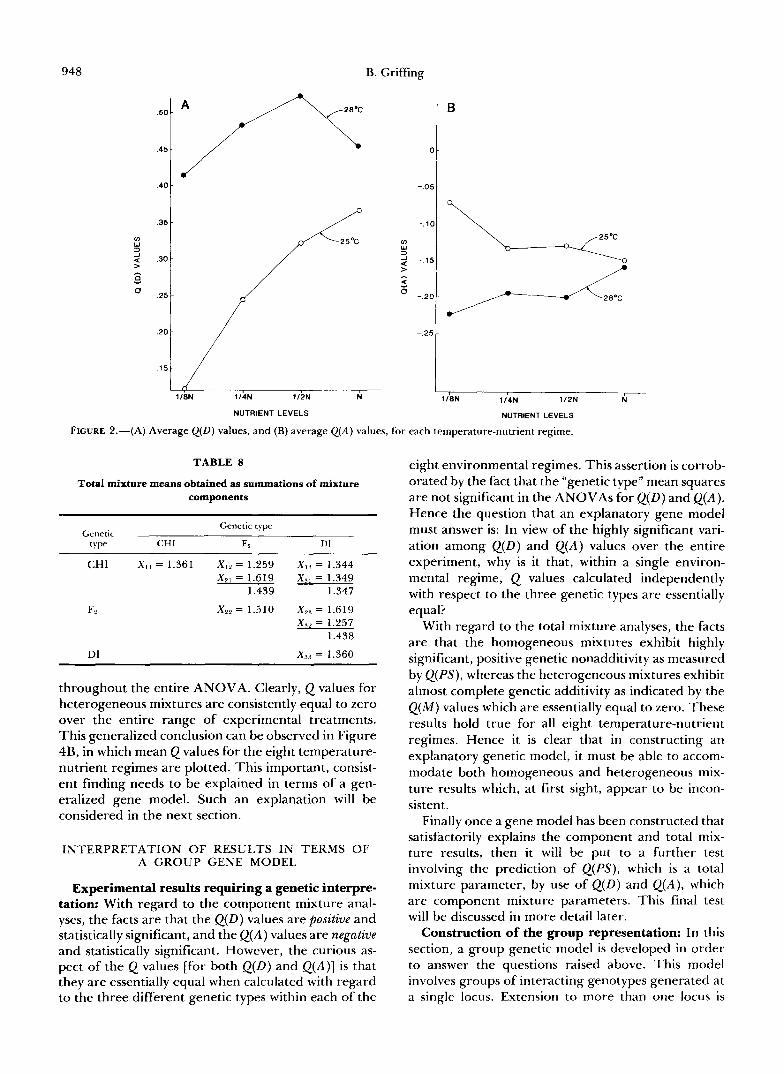
Q(D) values tend to increase with increased nutrients, and the mean square for nutrient levels is highly significant. Therefore the Q(D) data also illustrate a nutrient-dependent form of genetic nonadditivity. The significant TXN interaction mean square indicates that temperature responses are not entirely consistent at various nutrient levels. From Figure 2A, it is apparent that the discrepant value appears to be at the highest nutrient level, N.

The analysis of variance for the associate measure of nonadditivity, Q(A) , is presented in Table 7. The only significant mean square is that due to temperature. Thus the associate form of genetic nonadditivity is temperature-dependent. Figure 2B presents the average responses of Q(A) for each of the temperature- nutrient regimes. This figure illustrates that all Q(A) values are negative, and that the values at 28" are more extreme than those at 25".

It is clear from Figure 2, A and B, that the Q(D) and Q(A) values differ in qualitative and quantitative ways: Q(D) is positive and Q(A) is negative; Q(D) is of greater magnitude than Q(A). However, there is one important characteristic that they have in common. In the ANOVAs for both Q ( D ) and Q ( A ) , the mean squares for "genetic type" are nonsignificant (see Table 7). This implies that Q values estimated for each genetic type (CHI, F2 and DI), within each temperature-nutrient regime, are essentially equal. Hence, apparently, the genetic type does not influence the Q(D) [or Q(A)] value with which it is associated.

Analyses of total mixture responses: In previous sections, the individual mixture components were analyzed. In this section the components are combined to yield total mixture responses as the basis for analysis.

T o introduce the notion of total mixture response, consider the example given in Table 4. The mixture component means of Table 4 are combined to give the appropriate total mixture means as listed in Table 8. There are two classes of mixtures represented in Table 8: (i) homogeneous (pure-stand) mixtures; these include CHI, FB, and DI pure stands, the means of which are: CHI = 1.36 1, FB = 1.5 10 and DI = 1.360, and (ii) heterogeneous mixtures; these include the (CHI, FY), (CHI, DI), and (F2, DI) combinations. Means for

heterogeneous mixtures are (CHI, Fz) = 1.439, (CHI, DI) = 1.347 and (F2, DI) = 1.438.

In the following analyses, which include all eight environmental regimes, the homogeneous and heterogeneous mixtures are presented separately. Homo- geneous mixtures are those in which the two plants in a test tube are of the same genetic type. Designation of the three types is shortened to CHI, Fz and DI pure stands. Mean yields of the pure stands for each nutrient level at 25 ' are given graphically in Figure 3A, and at 28" in Figure 3B. These figures indicate that a very considerable amount of genetic nonadditivity is expressed among the homogeneous mixtures. A more critical analysis of the nonadditive responses is made by use of the Q measure which is calculated as follows:

Q(PS) = 2(FZ,F2) - [(CHI, CHI) + (DI, DI)].

A factorial ANOVA for the Q(PS) values is given in Table 9. It is clear that the mean squares for temperatures and nutrient-levels are significant. Therefore, nonadditivity measured among pure stands is both temperature- and nutrient-dependent. The increased (2 values at higher temperatures, and also at higher nutrient levels, can be observed in Figure 3C, in which Q(PS) values are plotted for each temperature-nutrient regime.

Heterogeneous mixtures are defined as those in which the two mixture components are derived from different genetic types. The experimental results indicate that heterogeneous mixture responses are fun- damentally different from those of homogeneous mixtures. Homogeneous mixtures exhibit a large amount of genetic nonadditivity; heterogeneous mixtures exhibit complete additivity. As an illustration, consider yields of (CHI, F2) and its component pure stands for all nutrient levels at 28 O , which are plotted in Figure 4A. The (CHI, F2) mixture yields are strictly inter- mediate. Similar responses occur for all heterogeneous mixtures in the various environmental regimes. A Q measure can be used again to analyze, more critically, the extent of nonadditivity of mixture responses. For example, the Q measure for (CHI, F2) is defined as follows:

Q ( M ) = 2(CHI, F2) - [(CHI, CHI) + (F2, F2)].

A factorial ANOVA for heterogeneous Q values is given in Table 9. The nonsignificant mean square for mixtures in the ANOVA indicates that all heterogeneous mixtures exhibit a strictly additive relationship with respect to the pure stands of their component genetic types. Furthermore, heterogeneous mixture responses remain additive at all temperature-nutrient regimes; as indicated by nonsignificant temperature and nutrient mean squares. In fact, the remarkable aspect of the ANOVA for heterogeneous mixtures in Table 9 is that there are no significant mean squares

948 B. Griffing

.50 -

.45 -

.40 -

3 5 -

.30 -

2 5 -

20 -

15 -

- 1 18N 114N 112N N

NUTRIENT LEVELS

0 -

15 -

10-

15-

10

!5 -

- 1

B

18N 114N 112N N

NUTRIENT LEVELS

FIGURE 2.-(A) Average Q(D) values, and (B) average Q ( A ) values, for each temperature-nutrient regime.

TABLE 8

Total mixture means obtained as summations of mixture components

Genetic Genetic type

‘Y Pe CHI F, DI

X,, = 1.619 X,, = 1.349 1.439 1.347

DI X:<, = 1.360

throughout the entire ANOVA. Clearly, Q values for heterogeneous mixtures are consistently equal to zero over the entire range of experimental treatments. This generalized conclusion can be observed in Figure 4B, in which mean Q values for the eight temperature- nutrient regimes are plotted. This important, consistent finding needs to be explained in terms of a generalized gene model. Such an explanation will be considered in the next section.

INTERPRETATION OF RESULTS IN TERMS OF A GROUP GENE MODEL

Experimental results requiring a genetic interpretation: With regard to the component mixture analyses, the facts are that the Q(D) values are positive and statistically significant, and the Q ( A ) values are negative and statistically significant. However, the curious aspect of the Q values [for both Q(D) and Q ( A ) ] is that they are essentially equal when calculated with regard to the three different genetic types within each of the

eight environmental regimes. This assertion is corroborated by the fact that the “genetic type” mean squares are not significant in the ANOVAs for Q ( D ) and Q(A). Hence the question that an explanatory gene model must answer is: In view of the highly significant variation among Q(D) and Q(A) values over the entire experiment, why is it that, within a single environmental regime, Q values calculated independently with respect to the three genetic types are essentially equal?

With regard to the total mixture analyses, the facts are that the homogeneous mixtures exhibit highly significant, positive genetic nonadditivity as measured by Q(PS), whereas the heterogeneous mixtures exhibit almost complete genetic additivity as indicated by the Q ( M ) values which are essentially equal to zero. These results hold true for all eight temperature-nutrient regimes. Hence it is clear that in constructing an explanatory genetic model, it must be able to accommodate both homogeneous and heterogeneous mixture results which, at first sight, appear to be incon- sistent.

Finally once a gene model has been constructed that satisfactorily explains the component and total mixture results, then it will be put to a further test involving the prediction of Q(PS), which is a total mixture parameter, by use of Q(0) and Q(A) , which are component mixture parameters. This final test will be discussed in more detail later.

Construction of the group representation: In this section, a group genetic model is developed in order to answer the questions raised above. This model involves groups of interacting genotypes generated at a single locus. Extension to more than one locus is


B / l.80i A 1.60

\ F2 Pure Stand

.os -

1.55 - F2 Pure Stand

CHI Pure Stand 1.50 - .25

0 1.45

Dl Pure Stand $ 1.45-

2 U 1.40 U. 1.40 - Dl Pure Stand

s s 1.35 1.35 -

.10

1.30 1.30 - .05 -

1.25 1.25.

0 ; l I 8 N 1/4N 112N N l l8N 114N 112N N 118N 114N 112N N

NUTRIENT LEVELS NUTRIENT LEVELS NUTRIENT LEVELS

FIGURE 3.-Yields of homogeneous mixtures (pure stands): (A) at 2 5 " . and (B) at 28", for each nutrient level, (C) Q(PS) values for each temperature-nutrient regime.

A

1 601

1/8N 1 /4N 112N N

B

- N 1 /8N 114N 112N

NUTRIENT LEVELS NUTRIENT LEVELS

FIGURE 4.-(A) Yields of the heterogeneous mixture (CHI, FY) and its associated pure stands; (B) Q ( M ) values for each temperature- nutrient regime.

discussed later. The genetic design of this study incor- porates two homozygous races and their FP. With regard to a single locus, the design dictates use of a model involving two equally frequent alleles. Hence the genotypic array for the conceptual base population is:

(1/4)(A,AI + A1AP + APA1 + A2A2).

Since the genetic design also utilizes groups of size two, it is necessary to generate a population of random groups of size two from the base population. This can be accomplished by "squaring" the base array as fol-

lows:

The direct-associate matrix of genotypic values for such a population of groups is illustrated in Table 1 0 , where, for example; qGkL = genotypic value for AJ, when associated with AkAl in groups of size two.

Relationships between experimental and group representations: In order to interpret the experimental results in terms of group genetic parameters, it is necessary to establish relationships between experimental and group genotypic values. In working out

950 B. Griffng

TABLE 9

ANOVAs of Q values for homogenous and heterogenous mixtures

Q(P.S): homogenous mixtures Q(A4): heterogenous mixtures

Source df Mean squares Source df Mean squares

Replications ( R ) 1 0.00032 NS Mixtures ( M ) 2 0.00045 NS Temperatures ( r ) 1 0.07426*** Temperatures ( r ) 1 0.000 10 NS

Nutrients ( N ) 3 0.01304* Nutrients ( N ) 3 0.00050 NS R X T 1 0.00087 NS M X T 2 0.00005 NS R X N 3 0.00036 NS M X N 6 0.00045 NS T X N 3 0.00281 NS T X N 3 0.001 73 NS R X T X N 3 0.00062 M X T X N 6 0.00073


TABLE 10

Direct-associate matrix of genotypic values

Associate genotypes Direct

genotypes A , A , AIA2 A2AI AzAz Mean

A I A I I I G I I , , G I , I I G I IIGPP I I G . . A I A Z I & , , I & I ~ ~ & n n I & .

A& 1 Y I G I I ~ I G ~ P 2tG2t 2 1 G z nlG.. A2A2 n&11 P P G ~ P ,&,I n&nn n L . .

Mean . . G I , . . G I 2 . . G I . . G Z 2 ..e.. = p

these relationships it must be remembered that the F p , rather than the F1, generation is used. The relationships are as follows ( E symbolizes “expectation” in the statistical sense).

E(X1 1 ) = 1 IGI I

~ ( ~ 1 2 ) = ( ~ / ~ ) ( 1 1 ~ 1 1 + 1 1 Q 1 2 + 1 1 G 2 1 + 1 1 G 2 2 ) = 1 I G . .

E(XI J) = I I Gn2

E ( X ~ I ) = ( ~ / ~ ) ( I I G I I + I & I I + ~ ~ G I I + ~ & I I ) = . . G I I

E(X,, )= . .G. . = p

E(X23) = ( 1 /4)( I I G 2 2 + I 2 G 2 2 + 21G22 + 2 2 6 2 2 ) = . . G 2 2

E(&,) = 2 2 G l l

E ( ~ R S ) = ( ~ / ~ ) ( ~ & I I + n & 1 2 + 2 & 2 1 + 2 2 6 2 2 ) = 2 & . .

E(&$) = 2 2 G 2 2 .

The next step is to evaluate the various measures of genetic nonadditivity in terms of group genotypic values. The expected Q(D) value when calculated with respect to the kth associate background is:

E[Q(Dk)] = E[2X2k - (Xlk + X M ) ] .

Expectations for the three values of k are:

E[Q(D,)]=~(..G,I)--(IIGII + P & I I ) ,

E[Q(&)] = 2(. .G22) - ( I 1Gn2 + 22G22). I E[Q(D2)]=2(..G..)-(11G..+22G..),and ( 1 )

The expected Q ( A ) value when measured with regard

to the ith direct genotype is:

E[Q(Ai) = E[2Xt2 - ( X I + X ~ S ) ]

Expectations for the three values of i are:

E[Q(AI)]=~(~IG..)-(IIGII + 11Gzz),

E[Q(A2)] = 2(. .G. .) - (. .GI 1 + . .G22), and (2)

E[Q(As)J = 2(22G. .) - (zzG1 I + 22G22) . I The genetic nonadditivity as expressed with pure stands is:

E[Q(PS)] = E[2X22 - ( X I I + Xm)]

=[2(..G..)-(11G11 + 2 2 G 2 2 ) ] .

Q values for the three heterogeneous mixtures are evaluated as follows:

(i) ( C H I , DI) mixture:

E[Q(M)] = E [ ( X I , + X ~ I ) - ( X , I + X,,)]

= ( I 1G2z + 1 ) - ( I I G I I + 2 d h )

(ii) ( C H I , F2) mixture:

E[Q(M)] = E[(X12 + X21) - (XI 1 + X22)]

=(11G.. + . . G I I ) - ( I I G ] I + . . G . . ) .

(iii) (DI, F2) mixture:

E[Q(M)] = E[(X32 + X ~ B ) - (X22 + X ~ T ) ]

= nnG.. + , .G22 - (22G22 + . . G . .).

Construction of the group gene model: In order to interpret the Q values (listed above) in terms of genetic effects, it is necessary to construct a genetic model to be associated with the group genotypic values (vGkl). These values can be characterized by genetic models at two levels ( i e . , at genotypic and gene levels).

Genotypic model:

VCR/ = P + Dy + Ah/ + (DA)tjk/,

where

/1 = . .G.. = population mean,

Genetic Analysis of Plant Mixtures 95 1

,,G. . - p = direct effect of genotype AJ,,

. . GkI - p = associate effect of genotype A J I , and

,,GIl - p - D, - Akl = interaction effect between direct genotype A, AI and associate genotype A&.

Gene model: The genotypic model can be partitioned further into a gene model as follows:

,,Gk/ = p + di + d, + (dd)q + ak + Ul + (UU)k l + (dU),k

+ (da),l + (dU)jk + (da)jl + (dUU)ikl + (daa)jk/ ( 3 )

+ (ddU),k + (dda)q/ + (ddUU)+/

z . G . . - 1.1 = direct additive effect of Ai, ( l jG. . - p - d , - dj ) = direct dominance effect of AiAl, . .Gk. - p = associate additive effect of Ak, (. .Gk/ - p - ak - al) = associate dominance effect of AkAI.

All remaining effects in the gene model are interaction effects between direct and associate genes and/ or genotypes.

With two equally frequent alleles, the restrictions on direct and associate main effects are simply:

d l + d , = 0, Zj(dd) , = 0, for all i , and Zi(dd), = 0, for allj.

a l + a 2 = 0 , Zj(aa)q = 0, for all i; and Zi(aa), = 0, for allj.

Elements in the two models can be related as follows:

Dg = d, + d, + (dd), ,

= Uk + al + (UU)kl.

(DA)ekr = (da),k + * * + (ddaa),jkl

= sum of all interaction effects.

For a further elaboration of the group model see GRIFFING (1 98 1 a).

Evaluation of Q values and interpretation of experimental results: Before evaluating the Q values, it is useful to simplify the group gene model, ( 3 ) , in accordance with the experimental results. The basic information required for judging which elements should be included in the model is given in the AN- OVAs listed in Tables 5 and 6. The patterns of statistical significance for mean squares, MS(D) , MS(A) , and MS(DA), over all eight regimes, are as follows:

1. Direct mean squares, MS(D) , are consistently, highly significant. Therefore,

D,, = d , + d, + (dd) , ,

should be included in the model.

2 . Associate mean squares, MS(A) , are consistently, highly significant. Therefore,

Akl ak + ai + (aa)k/,

should be included. 3 . However, direct X associate mean squares,

MS(DA), are nonsignificant in essentially all treatment regimes. This implies that the interaction effects,

(DA)qk/ = (dU),k + - - - + (ddaa)qkl,

can be ignored.

model simplifies to, Based on these statistical results, the group genotypic

= I.1 + D, + Akl, (4)

and the gene model becomes,

qCkl= 1.1 + di + dj + (dd)o + Uk + al+ ( U U ) k l . ( 5 )

This model could be simplified even further by considering the linear and quadratic components of MS(D) and MS(A) . However, models (4) and (5) are used in order to provide a more generalized result, which demonstrates independence of additive and nonadditive (dominance) effects in the Q measures.

It is now possible to evaluate the Q values in terms of the simplified genetic models as follows:

The expected Q ( D ) parameters, in terms of the group genotypic values, are given in (1). For all values of k, these become,

E[Q(Dk)] = -(Dl 1 + O 2 2 ) (6) = - [ 2 d l + ( d d ) , , + 2d2 + (dd)22].

When the restrictions on gene effects are applied, (6) becomes,

E[Q(Dk)] = 2(dd)12, fork = 1 , 2 , 3 . (7)

Thus, although the three functions in (1) are different for the three associate backgrounds (i.e., k = 1, 2 , 3), they all yield the same result, (7), with the simplified gene model (5). This demonstrates that Q ( D ) values calculated for each associate background within each of the eight environmental regimes should be approximately equal. Thus one of the puzzling experimental results is solved. The second important point with regard to (7) is that Q ( D ) values are functions of only direct dominance effects. Perhaps this becomes more clear if the results of (7) are transformed into a different diallelic model in which the direct genotypic values are: A I A I , ( d ) : AlA2 (or AZAI), (h,): and A2A2, ( - d ) . In this model the genotypic value, “h,,” is a measure of the deviation of the direct heterozygote from its mid- parental value. With gene frequencies equal to one- half, 2(dd)12 = h,, and (7) becomes simply, E[Q(D) ] = h,. Finally, Q ( D ) values can change from one temperature-nutrient regime to another. Such changes are a reflection of the phenomena of temperature- and/or

v

952 B. Griffing

nutrient-dependent heterosis. Both forms of heterosis were found to be highly significant in Table 7.

The expected Q(A) parameters, in terms of the group genotypic values, are given in (2). In terms of the gene model, these all become,

E[Q(AJ] = (AI I + A22)

= 2(UU)l2 (8 )

= h A , i = 1 , 2 , 3 .

As with Q(D) values it is clear that: (i) The result, (8), holds for any of the three direct genetic types; this fact is responsible for the nonsignijicunt mean square attributable to “genetic type” in the ANOVA for Q(A) in Table 7, and thus, the second puzzling experimental result is explained. (ii) The result, (8), demonstrates that genetic nonadditivity measured by Q(A) is strictly a measure of heterosis in the associate dimension of gene activity. (iii) Q(A) values can, and do, change when measured in different temperature-nutrient regimes. The highly significant mean square in Table 7 indicates that this form of heterosis is temperature- dependent.

The third puzzling aspect of the experimental data was the fact that although there was considerable manifestation of genetic nonadditivity in mixture components, the Q ( M ) values for heterogeneous mixtures were all essentially equal to zero. Thus heterogeneous mixtures exhibited complete additivity. T o explain this phenomenon it is necessary to evaluate the Q(M)s in terms of the group genetic models [(4) and (5)]:

(i) (CHI, DI) heterogeneous mixture. [Q(CHI, Dl)] = ( I 1Gz2 + 22G1 I ) - ( I I G I I + 22G22)

=[ (P+DII +A‘L~)+(P+&: !+AII ) ]

= 0. - [ ( P + + I I + A ~ I ) + ( P + & + A ~ ~ ) ]

(ii) (CHI, F2) heterogeneous mixture.

E[Q(CHI,F2)]=(llG.. + . .GII)-(lIGII + . .G. . ) = [ ( P + ~ l I ) + ( P + A l I ) l

- [ ( P + + I I + A I I ) + P ] = 0.

(iii) (DI, F2) heterogeneous mixture.

E[Q(DI, Fz)] = (22G.. + . .G22) - (22G22 + . .G. .) = [(P + 0 2 2 ) + (P + AzJ)] - [(P + D22 + A22) + PI

= 0.

These results indicate that the group genetic model can accommodate any degree of genetic nonadditivity in the direct and associate dimensions of gene expression, while at the same time exhibit complete additivity, with regard to the interaction between genotypes within groups. Hence the model that has been constructed completely describes the experimental results

obtained with regard to the Q(D), Q(A) and Q(M) parameters.

Prediction of the Q(PS) parameter: Finally, it is possible to put the genetic model to an independent test. This test involves the Q parameter for homogeneous mixtures, Q((PS), which is evaluated in terms of the gene model as follows:

E[(L(PS)]=2(..G..)-(,IG11 +22G22) = [ ~ ( c L ) ] - [(P + DI I + A I I ) + (P + 0 2 2 + A22)]

-[(Dl1 +&)+(Al l +A22)] = h, + h,.

If the group theory is correct, and the group gene model is useful in describing genetic nonadditivity in the experimental system, it should be possible to pre- dict Q(PS) by the following relationship of Q values:

Q(PS ) = Q(D ) + Q(A ). Validity of this prediction can be observed in Figure 5A which presents average Q values for each nutrient level at 2 5 O , and Figure 5B which gives Q values for each nutrient level at 2 8 O . These figures illustrate the remarkable coincidence of Q((PS) and its predictor, [Q(D) + Q(A)], over the entire range of temperature- nutrient regimes. Hence the predictive nature of the group genetic model is demonstrated.

DISCUSSION

Restatement of problem and method of attack The basic objective of this study is to provide a genetic analysis of responses to interacting genotypes in biological groups which were subjected to a range of environmental conditions. The experimental procedure involved growing all possible pairwise combinations of plants, from two different races and their hybrid, in test tubes which were subjected to exactly controlled environmental conditions.

Genetic analyses of such mixtures are complicated by the fact that plants within groups may interact, i e . , they may influence each others’ growth responses, especially when the plants are competing for limited environmental resources. This implies that a particular genetic type may yield quite differently depending on the associate genetic type with which it is grown. Such a complication creates a difficult problem of interpretation in terms of the classical (noninteraction) quantitative genetic theory.

An outline of the method of attack used in this study is as follows: (i) Recognize that a group gene model [as set out in ( 3 ) ] has been specifically designed to accommodate interactions between individuals within groups. This model is suitable for the genetic design in this study. (ii) Recognize that a one-to-one correspondence exists between classes of gene model effects and the eight comparisons responsible for an orthogonal partitioning of the total variation in a 2” factorial ANOVA of the direct-associate pattern of means. Such a correspondence is illustrated in Table


.35 -

.25

(0 1 5 - 3 J

J . 05 -

- 251- ! 118N 114N 112N N

NUTRIENT LEVELS

118N 114N

NUTRIENT LEVELS

FIGURE 5.-Comparison of Q(PS) with the predicted value given by [Q(D) + Q(A)] for each nutrient level: (A) at 2 5 " , and (B) at 28".

TABLE 11

Correspondence of classes of gene model effects and ANOVA comparisons

Gene model effects ANOVA comparisons

,GI/ P (population mean)

+(d, + d,) (direct additive) w4 (direct linear)

+ ( d 4 , (direct dominance) q(D) (direct quadratic) + (ak + a/) (associate additive) 4 4 (associate linear)

+ (aa),, (associate dominance) q ( 4 (associate quadratic) + [(da)$k + . . . + (da)~, ] (additive X additive) V ) x 4 4 ) (linear X linear) + [(daa)iM + (daa)Jk/] (additive X dominance) 4 4 x q ( 4 (linear X quadratic) + [(dda)yk + ( d d a ) ~ ~ ! ] (dominance X additive) x 4 4 (quadratic X linear) + (ddaa)ykl (dominance X dominance) q(D) x q(A) (quadratic X quadratic)

11. This ANOVA also provides the appropriate method for statistically testing the contribution of each class of gene effects with respect to genetic variation in the direct-associate pattern of data. It is clear then, that in the above method of attack, the key is the recognition of the one-to-one relationship between ANOVA comparisons and classes of gene effects. Hence the operational procedure is to per- form the direct-associate ANOVA and determine which of the eight orthogonal comparisons are significant. Then the statistically significant comparisons, themselves, are used to characterize the contributions of the specific classes of gene effects to the genetic variation in the experimental material.

The above argument holds perfectly for the situa- tion in which the experimental procedure utilizes the F1 generation resulting from crossing two homozygous parents. However when the F2 generation is used, as in this study, certain modifications need to be made in the analysis. Earlier, it was demonstrated that in the absence of direct x associate interaction effects, quadratic comparisons yielded unbiased estimates of

dominance parameters. However, when direct X associate interaction effects cannot be ignored, the procedure must be slightly modified, when F2 data are used. In this case it is necessary, first, to identify the different possible linear and quadratic comparisons as

MD1)=2X21 "(X11 +XN)

Q(D3) = 2x23 - (X13 +&S)

954 B. Griffing

Using these linear and quadratic contrasts of experimental means, the eight orthogonal comparisons can be determined which, in turn, provide unbiased estimates of the corresponding class of gene effects. These may be summarized as follows:

Main effects :

1 . Direct additive, (dJ: 1(D) = kIL(D2) 2. Associative additive, (ak): 1(A) = kIL(A2) 3. Direct dominance, [ ( & Q j ] : q ( D ) = k 2 Q W 4. Associate dominance, [(aa)kl]: q(A) = kzQ(A2)

Interaction effects:

5 . Additive X additive, [(da);k]:

l ( D ) X I(A) = ~ : ~ [ L ( D I - L(D3)] = ~B[L(AI) - L(AB)]

6. Additive X Quadratic, [ (daa)~]:

1(D) X q(A) = k4(2L(D2) - [L(DI) + L(&)]]

= k4[Q(Al) - Q(AB)]

7. Quadratic X Additive, [(dda),k]:

q(D) x 4 4 ) = MQ(D1) - Q ( W 1 = k5(2L(A2) - [ (LA, ) + L(A3)IJ

8. Quadratic X quadratic, [(ddaa),kl]:

do) x !?(A) = k6(2Q(D2) - [ Q W + Q(D3)IJ = k6(2Q(A2) - [Q(AJ + Q(Ad1J.

In the above representation, the k’s are appropriate constants.

Further points of interest with regard to the complete model and use of F2 data are:

1.

2.

The quadratic measure for homogeneous mixtures can be predicted as:

Q(ps) = Q(&) + Q(A2) + Q(CH1, F2) + Q(D1, F2).

The quadratic measures for heterogeneous mixtures, Q(CH1, F2), Q(D1, F2) and Q(CH1, DI), are functions of only direct X associate interaction effects. This implies that a better than average yield for these heterogeneous mixtures requires nonadditive interactions between genes in different genotypes within groups.

Finally, the theory developed in the above analyses is based on genotypes segregating at a single locus. When several independent segregating loci contribute to the total genetic variability, the orthogonal comparison for a particular class of gene effects becomes the sum of those effects from each locus.

Review of experimental results. With regard to the experimental results of this study, the ANOVAs yielded consistent results over all environmental regimes. These results are summarized briefly as follows:

1 . Direct ( D ) mean squares were highly significant

over all regimes. This implied that genotypes of the three genetic types differed significantly in their direct contributions to mixture yields. Fur- ther partitioning of the direct variation into linear and quadratic components, consistently, demonstrated that essentially all of the direct variation was nonadditive. Associate (A) mean squares were highly significant. This implied that individuals within groups inter- fered with each others’ growth responses, i.e. the three genetic types of associate members differentially influenced yields of the direct group members. Further partitioning of the associate variation, again, indicated that most variation over all regimes was nonadditive. Direct X associate (DXA) mean squares were consistently nonsignificant. Thus, although yields of all genetic types were differentially influenced by associate genotypes, a direct x associate, nonadditive interaction did not exist. The conclusion from these basic analyses was that the only effects in the gene model that significantly contributed to the genetic variation of the experimental results were the direct and associate heterosis effects.

Having identified the classes of gene effects that - -

caused genetic variation in the experimental material, the final step was to characterize these effects in qualitative and quantitative terms. This was accomplished by use of the appropriate quadratic contrast, Q(D), which measured the total heterosis in the direct dimension, and Q(A), which did the same in the associate dimension. The two kinds of heterosis differed qualitatively (direct heterosis was positive whereas associate heterosis was negative) and quantitatively (the magnitude of direct heterosis was greater than that of associate heterosis).

Biological interpretation of the experimental results: The previous sections summarized the analytical method of attack and the basic experimental results. A biological interpretation of these results is now considered. The positive, significant Q(D) values indicate that the F2 exhibits greater yield than either parental race when grown with any of the three associate genotypes. This is true for all temperature-nutrient regimes. Hence the F2 exhibits a higher growth rate than those of the parental races over the given time period for each and every environmental regime. The negative, significant Q(A) values can be explained in terms of the higher F2 growth rate and the fact that nutrients available to the plants in a test tube are limited. When the F2 competes with a parental race for the limited supply of nutrients, the F2, because of its higher growth rate, utilizes more than its share of nutrients and thereby forces the parental race to grow on a reduced nutrient supply. In all cases, this results in an increased F1 yield at the expense of that of the


parental race. Therefore a negative Q(A) value is produced.

The above explanation for positive Q(D) and negative Q(A) values implies that a negative relationship between these two classes of effects should exist. The highly significant correlation coefficient for Q(D) and Q(A) values, averaged over all genetic types for each temperature-nutrient regime, is: r = -0.88. Thus there does exist a close, negative relationship. The regression equation expressing this relationship is:

Q(A)= -0.041 - 0.32Q(D).

Hence the magnitude of the predicted Q(A) values are approximately one-third that of the Q(D) values.

The temperature-dependent nature of the direct and associate expression of heterosis is of special interest. Comparison of Figures 3A and 3B indicate that yields of parental races drop considerably more than yields of the FP, when the temperature is raised from 25" to 28". This differential response can be examined more critically by recording differences in yield between 25' and 28" for each genetic type at each nutrient level. These data give the average F2 drop as 0.047 and the average decrease for the two races as 0.1 15. Hence the parental decrease is approximately 2.5 times as great as that for the FP. Furthermore, the difference is, statistically, highly significant. This temperature induced differential decrease in yield, when a hybrid is compared with its parents, suggests that each parent has a set of temperature-sensitive genes which are somewhat different in the two races. In the hybrid, then, some of the temperature-sensitive alleles of one parent are compensated for by non-temperature-sensitive alleles of the other parent. A temperature-dependent heterosis results.

This phenomenon has been reported in Arabidopsis before (LANCRIDCE and GRIFFINC 1959; GRIFFINC and LANGRIDCE 1963; GRIFFINC and ZSIROS 197 l), and in maize (MCWILLIAM and GRIFFINC 1965). The suggested solutions of either replacing temperature- sensitive by non-temperature-sensitive alleles, or, in more complicated cases by making use of hybrids, have been made in the above references.

Further aspects of the modeling process; historical notes: The group genetic model was first proposed (GRIFFINC 1967) in response to a plant breeding dilemma. This dilemma was brought into sharp focus by WIEBE, PETR and STEVENS (1963) in an international plant breeding conference. The classical selection theory could not solve the problem because it could not cope with genotypic interactions. The first step of a theoretical solution was to develop a modeling system that could accommodate genotypic interaction, and then to use this modeling system to search for selection procedures that circumvented the dilemma and produced the desired results. A series of additional studies were devoted to this effort (GRIFF- ING 1968a,b, 1969; 1976a,b; 1977). Other authors

[GALLAIS (1976) and WRIGHT (1982, 1983, 1986), among others] have used the group genetic model with regard to plant breeding problems.

Another series of studies utilized the same group genetic model in order to examine various aspects of the evolution of social behavior (GRIFFINC 198 1- a,b,c,d; 1982a,b,c,d,e,f). These studies explored, in depth, the various kin- and group-selection strategies that are usually considered in the context of the evolution of social behavior.

Further aspects of the modeling process; proper- ties of the group genetic model: In addition to accom- modating genotypic interaction, the model was designed specifically to be an extension of the classical (noninteraction) quantitative genetic model. Thus a generalized quantitative genetic modeling system was constructed which ensured that: (i) the group (interaction) model collapsed to the classical (noninteraction) model in the absence of genotypic interaction; (ii) as with the classical model, the group representation accommodated any number of alleles with arbitrary gene frequencies, and any set of dominance parameters for genotypes at a single locus; extension to more loci was, of course, possible; (iii) the group model retained the important property of the classical model with regard to characterizing the results of selection: it exactly identified and isolated appropriate gene effects and variance components that entered into the description of changes in gene frequencies and the population mean. This property was abso- lutely essential in all of the theoretical studies reported above.

Finally the group modeling scheme was designed to accommodate groups of arbitrary size, and nonran- dom as well as random groups.

Rationale of the present study: All studies listed in the above historical account were theoretical in nature. There does not appear to be any study that tests the validity of the model with data from a living system. Such a description should involve effects rather than variance components because qualitative (positive or negative) as well as quantitative (magnitude) attributes of the model are important. Hence the main objective of the present study was to set up an experimental procedure that permitted the exam- ination of the usefulness of the various classes of model effects in describing the complex variability generated by interacting genotypes within a living system.

The simplest experimental procedure was to plant all possible pairwise combinations of two different homozygous parents and their hybrid. Such a design yielded a direct-associate pattern of means that was appropriate for the analysis of any quantitative locus whose genotypes differed in the parental material. Using the orthogonal partitioning associated with this 23 factorial arrangement provided the statistical tools for the identification, testing and estimation of all

956 B. Griffing

classes of effects in the group genetic model. The present study, then, utilized this experimental approach in an endeavor to test the group genetic model with data from a bona fide living system.

LITERATURE CITED

BARRETT, J. A., 1981 The evolutionary consequences of mono- culture, pp. 209-248 in Genetic Consequences of Man Made Change, edited by J. A. BISHOP and L. M. COOK. Academic Press, New York.

CLAY, R. E., and R. W. ALLARD, 1969 A comparison of the performance of homogeneous and heterogeneous barley populations. Crop Sci., 9: 407-412.

GALLAIS, A., 1976 Effects of competition on means, variances and covariances in quantitative genetics with an application to general combining ability selection. Theor. Appl. Genet. 47: 189- 195.

GRIFFING, B., 1967 Selection in reference to biological groups. I. Individual and group selection applied to populations of unor- dered groups. Aust. J. Biol. Sci. 2 0 127-139.

GRIFFING, B., 1968a Selection in reference to biological groups. 11. Consequences of selection in groups of one size when evaluated in groups of a different size. Aust. J. Biol. Sci. 21: 1163-1 170.

GRIFFING, B., 196% Selection in reference to biological groups. 111. Generalized results of individual and group selection in terms of parent-offspring covariances. Aust. J. Biol. Sci. 21: 1171-1178.

GRIFFING, B., 1969 Selection in reference to biological groups. IV. Application of selection index theory. Aust. J. Biol. Sci. 22: 131-142.

GRIFFING, B., 1976a Selection in reference to biological groups. V. Analysis of full-sib groups. Genetics 82: 703-722.

GRIFFING, B., 1976b Selection in reference to biological groups. VI. Use of extreme forms of non-random groups to increase selection efficiency. Genetics 82: 723-73 1.

GRIFFING, B., 1977 Selection for populations of interacting genotypes, pp. 41 3-434 in Proceedings of the International Confer- ence on Quantitative Genetics, edited by E. POLLAK, 0. KEMP- THORNE and T . B. BAILEY. Iowa State Press, Ames.

GRIFFING, B., 1981a A theory of natural selection incorporating interactions among individuals. I. The modeling process. J. Theor. Biol. 8 9 636-658.

GRIFFING, B., 1981b A theory of natural selection incorporating interactions among individuals. 11. Use of related groups. J. Theor. Biol. 8 9 659-677.

GRIFFING, B., 1981c A theory of natural selection incorporating interaction among individuals. 111. Use of random groups of inbred individuals. J. Theor. Biol. 89: 679-690.

GRIFFING, B., 1981d A theory of natural selection incorporating interaction among individuals. IV. Use of related groups of inbred individuals. J. Theor. Biol. 89 691-710.

GRIFFING, B., 1982a A theory of natural selection incorporating interaction among individuals. V. Use of random synchronized groups. J . Theor. Biol. 9 4 709-728.

GRIFFING, B., 1982b A theory of natural selection incorporating interactions among individuals. VI. Use of non-random synchronized groups. J. Theor. Biol. 94: 729-741.

GRIFFING, B., 1982c A theory of natural selection incorporating interaction among individuals. VII. Use of groups consisting of one sire and one dam. J. Theor. Biol. 94: 951-966.

GRIFFING, B., 1982d A theory of natural selection incorporating interaction among individuals. VIII. Use of groups consisting of a sire and several dams. J. Theor. Biol. 94: 967-983.

GRIFFING, B., 1982e A theory of natural selection incorporating interaction among individuals. IX. Use of groups consisting of a mating pair and sterile diploid caste members. J. Theor. Biol. 95: 181-198.

GRIFFING, B., 1982f A theory of natural selection incorporating interaction among individuals. X. Use of groups consisting of a mating pair together with haploid and diploid caste members. J. Theor. Biol. 95: 199-223.

GRIFFING, B., and J. LANGRIDGE, 1963 Phenotypic stability of growth in the self-fertilized species, Arabidopsis thaliana, pp. 368-394 in Statistical Genetics and Plant Breeding, edited by W. D. HANSON and H. F. ROBINSON. NAS-NRC, Washington, D.C.

GRIFFING, B., and E. ZSIROS, 1971 Heterosis associated with genotypic-environment interactions. Genetics 6 8 443-455.

LANGRIDGE, J., 1957 The aseptic culture of Arabidopsis thaliana (L.) Heynh. Aust. J. Biol. Sci. 1 0 243-252.

LANGRIDGE, J., and GRIFFING, B., 1959 A study of high temperature lesions in Arabidopsis thaliana. Aust. J. Biol. Sci. 12: 117- 135.

MAYO, O., 1980 The Theory of Plant Breeding. Oxford University

MCWILLIAMS, J. R., and GRIFFING, B., 1965 Temperature-dependent heterosis in maize. Aust. J. Biol. Sci. 18: 569-583.

WIEBE, G. A., F. C. PETR and H. STEVENS, 1963 Interplant competition between barley genotypes, pp. 546-557 in Statis- tical Genetics and Plant Breeding, edited by W. D. HANSON and H. F. ROBINSON. NAS-NRC, Washington, D.C.

WRIGHT, A. J., 1982 Some implications of a first-order model of interplant competition for the means and variances of complex mixtures. Theor. Appl. Genet. 64: 91-96.

WRIGHT, A. J., 1983 The expected efficiencies of some methods of selection of components for inter-genotypic mixtures. Theor. Appl. Genet. 67: 45-52.

WRIGHT, A. J., 1986 Individual and group selection with competition. Theor. Appl. Genet. 72: 256-263.

Press, Oxford.

Communicating editor: M . TURELLI

Copyright 0 1989 by the Genetics Society of America

Gene Genealogy in Three Related Populations: Consistency Probability Between Gene and Population Trees

Naoyuki Takahata

National Institute of Genetics, Mishima, Shiruoka-Ken 41 I , Japan, and Center for Demographic and Population Genetics, The University of Texas Health Science Center, Houston, Texas 77225

Manuscript received November 2, 1988 Accepted for publication April 22, 1989

ABSTRACT A genealogical relationship among genes at a locus (gene tree) sampled from three related

populations was examined with special reference to population relatedness (population tree). A phylogenetically informative event in a gene tree constructed from nucleotide differences consists of interspecific coalescences of genes in each of which two genes sampled from different populations are descended from a common ancestor. The consistency probability between gene and population trees in which they are topologically identical was formulated in terms of interspecific coalescences. It was found that the consistency probability thus derived substantially increases as the sample size of genes increases, unless the divergence time of populations is very long compared to population sizes. Hence, there are cases where large samples at a locus are very useful in inferring a population tree.

T HE nucleotide differences among genes at a locus drawn from a species contain useful information

about how these genes evolved from a common ancestor. A genealogical relationship (gene tree) constructed from such nucleotide differences is a visual way of representing the evolutionary history of genes, through which not only the mechanisms of evolution of genes but also the evolutionary history of the species can be inferred. Furthermore, if orthologous (homologous) genes are drawn from different species or populations, the nucleotide differences can be used to infer the phylogenetic relationships of the species or populations (species or population tree).

However, even in the absence of gene flow, a gene tree does not necessarily show the same topological pattern as does a population tree (TAJIMA 1983; TAK- AHATA and NEI 1985; NEIGEL and AVISE 1986; NEI 1987). This discordance stems from the fact that orthologous genes in different populations generally diverged much earlier than population splitting. Tak- ing into account this possibility, NEI (1987) derived a simple formula for evaluating the probability that the topology of a tree for three orthologous genes, sampled from three different populations, is the same as that of the population tree. More recently, PAMILO and NEI (1988) extended the study of this problem to situations with more than three populations involved and those with more than one gene sampled from each population. They concluded that the consistency probability between gene and population trees becomes considerably smaller if internodal branches of

of page charges. This article must therefore be hereby marked “advertisement” The publication costs of this article were partly defrayed by the payment

in accordance with 18 U.S.C. 61734 solely to indicate this fact.

Genetics 122: 957-966 (August, 1989)

the population tree are short and that this probability cannot be substantially increased by increasing the number of genes sampled from a locus.

In this paper, I shall address the same problem as did PAMILO and NEI (1988), and show that their conclusion, which seems rather discouraging to exper- imentalists, is largely due to the limited study of small sample sizes and the criterion they used. It is important to clearly distinguish two qualitatively different nodes in a gene tree. Each node (coalescence in the mathematical study of genealogy) (KINGMAN 1982) corresponds to a bifurcation of a gene in the repro- duction process. A coalescence may be due to genes belonging to the same population or to different populations. These will be called intraspecific and interspecific coalescence, respectively. The occurrence of interspecific coalescence is a key event in a gene tree that can occur only before two populations involved have diverged from a common ancestor, and therefore it directly reflects population relatedness. Focus- ing on this event, I develop a theory relevant to the present problem and supplement the result with a simulation. It is then shown that sampling many genes from each population can indeed increase the consistency probability substantially, allowing us to correctly infer a population tree.

MODEL AND THEORY

The species considered here is monoecious and diploid. Generations are discrete and nonoverlapping, and for convenience they are counted backward chronologically from the present time. The species consists of three populations X , Y , and Z which se-

N. Takahata 958

4

2

time

11 +‘2

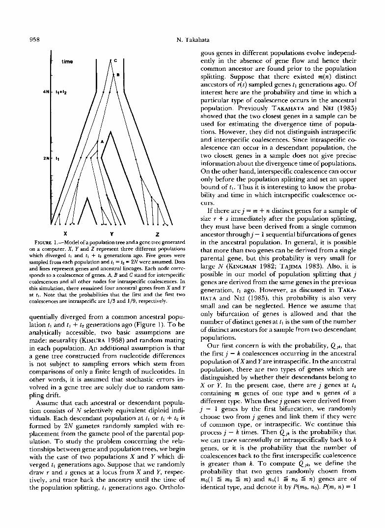
X Y FIGURE 1 .-Model of a population tree and a gene tree generated

on a computer. X , Y and Z represent three different populations which diverged t l and t l + t~ generations ago. Five genes were sampled from each population and tl = tn = 2N were assumed. Dots and lines represent genes and ancestral lineages. Each node corresponds to a coalescence of genes. A, B and C stand for interspecific coalescences and all other nodes for intraspecific coalescences. In this simulation, there remained four ancestral genes from X and Y at tl. Note that the probabilities that the first and the first two coalescences are intraspecific are 1/3 and 1/9, respectively.

quentially diverged from a common ancestral population tl and tl + t 2 generations ago (Figure 1) . T o be analytically accessible, two basic assumptions are made: neutrality (KIMURA 1968) and random mating in each population. An additional assumption is that a gene tree constructed from nucleotide differences is not subject to sampling errors which stem from comparisons of only a finite length of nucleotides. In other words, it is assumed that stochastic errors involved in a gene tree are solely due to random sampling drift.

Assume that each ancestral or descendant population consists of N selectively equivalent diploid individuals. Each descendant population at tl or tl + t2 is formed by 2N gametes randomly sampled with re- placement from the gamete pool of the parental population. T o study the problem concerning the relationships between gene and population trees, we begin with the case of two populations X and Y which diverged t l generations ago. Suppose that we randomly draw r and s genes at a locus from X and Y, respectively, and trace back the ancestry until the time of the population splitting, tl generations ago. Ortholo-

gous genes in different populations evolve independently in the absence of gene flow and hence their common ancestor are found prior to the population splitting. Suppose that there existed m(n) distinct ancestors of r(s) sampled genes t l generations ago. Of interest here are the probability and time in which a particular type of coalescence occurs in the ancestral population. Previously TAKAHATA and NEI (1985) showed that the two closest genes in a sample can be used for estimating the divergence time of populations. However, they did not distinguish intraspecific and interspecific coalescences. Since intraspecific coalescence can occur in a descendant population, the two closest genes in a sample does not give precise information about the divergence time of populations. On the other hand, interspecific coalescence can occur only before the population splitting and set an upper bound of t l . Thus it is interesting to know the probability and time in which interspecific coalescence occurs.

If there a r e j = m + n distinct genes for a sample of size r + s immediately after the population splitting, they must have been derived from a single common ancestor throughj - 1 sequential bifurcations of genes in the ancestral population. In general, it is possible that more than two genes can be derived from a single parental gene, but this probability is very small for large N (KINGMAN 1982; TAJIMA 1983). Also, it is possible in our model of population splitting that j genes are derived from the same genes in the previous generation, t l ago. However, as discussed in TAKA- HATA and NEI (1985), this probability is also very small and can be neglected. Hence we assume that only bifurcation of genes is allowed and that the number of distinct genes at tl is the sum of the number of distinct ancestors for a sample from two descendant populations.

Our first concern is with the probability, Q j r , that the first j - k coalescences occurring in the ancestral population ofXand Yare intraspecific. In the ancestral population, there are two types of genes which are distinguished by whether their descendants belong to X or Y. In the present case, there are j genes at t~ containing m genes of one type and n genes of a different type. When these j genes were derived from j - 1 genes by the first bifurcation, we randomly choose two from j genes and link them if they were of common type, or intraspecific. We continue this process j - k times. Then Q j k is the probability that we can trace successfully or intraspecifically back to k genes, or it is the probability that the number of coalescences back to the first interspecific coalescence is greater than k. To compute Q j k , we define the probability that two genes randomly chosen from mo(l d mo d m ) and no( 1 d no 5 n) genes are of identical type, and denote it by P(m0, no). P(m, n) = 1

genetic analysis of plant mixtures - genetics

Documents