genetic association - pennsylvania state university association monday, march 29, 2010. ... to share...

Genetic Association

Monday, March 29, 2010

Genetic Association Studies• Case-control designs

• Family based designs

• Quantitative trait association

- continuous trait

- longitudinal trait

©!!""6!Nature Publishing Group!

!

HaplotypeTyped marker locus Unobserved causal locus

Diseasephenotype

Indirectassociation

Directassociation

Directassociation

Significance levelUsually denoted !, and chosen by the researcher to be the greatest probability of type-1 error that is tolerated for a statistical test. It is conventional to choose ! = 5% for the overall analysis, which might consist of many tests each with a much lower significance level.

Test statisticA numerical summary of the data that is used to measure support for the null hypothesis. Either the test statistic has a known probability distribution (such as "2) under the null hypothesis, or its null distribution is approximated computationally.

Common-disease common-variant hypothesisThe hypothesis that many genetic variants that underlie complex diseases are common, and therefore susceptible to detection using current population association study designs. An alternative possibility is that genetic contributions to complex diseases arise from many variants, all of which are rare.

Effective population sizeThe size of a theoretical population that best approximates a given natural population under an assumed model. Human effective population size is often taken to mean the size of a constant-size, panmictic population of breeding adults that generates the same level of polymorphism under neutrality as observed in an actual human population.

Maximum-likelihood estimateThe value of an unknown parameter that maximizes the probability of the observed data under the assumed statistical model.

PhaseThe information that is needed to determine the two haplotypes that underlie a multi-locus genotype within a chromosomal segment.

Direct, laboratory-based haplotyping or typing further family members to infer the unknown phase are expensive ways to obtain haplotypes. Fortunately, there are statistical methods for inferring haplotypes and population haplotype frequencies from the geno-types of unrelated individuals. These methods, and the software that implements them, rely on the fact that in regions of low recombination relatively few of the possible haplotypes will actually be observed in any population. These programs generally perform well14, given high SNP density and not too much missing data. SNPHAP is simple and fast, whereas PHASE15 tends to be more accu-rate but comes at greater computational cost. Recently FASTPHASE has emerged16, which is nearly as accurate as PHASE and much faster.

True haplotypes are more informative than genotypes, but inferred haplotypes are typically less informative because of uncertain phasing. However, the informa-tion loss that arises from phasing is small when linkage disequilibrium (LD) is strong.

Note that phasing cases and controls together allows better estimates of haplotype frequencies under the null hypothesis of no association, but can lead to a bias towards this hypothesis and therefore a loss of power. Conversely, phasing cases and controls separately can inflate type-1 error rates. A similar issue arises in imputing missing genotypes.

Measures of LD and estimates of recombination rates. LD will remain crucial to the design of association stud-ies until whole-genome resequencing becomes routinely available. Currently, few of the more than 10 million common human polymorphisms are typed in any given study. If a causal polymorphism is not genotyped, we can still hope to detect its effects through LD with polymorphisms that are typed. To assess the power of a study design to achieve this, we need to measure LD. However, LD is a non-quantitative phenomenon: there is no natural scale for measuring it. Among the measures that have been proposed for two-locus haplotype data17, the two most important are D# and r2.

D# is sensitive to even a few recombinations between the loci since the most recent mutation at one of them. Textbooks emphasize the exponential decay over time of D# between linked loci under simple population-genetic models, but stochastic effects mean that this theoretical relationship is of limited usefulness. A disad-vantage of D# is that it can be large (indicating high LD) even when one allele is very rare, which is usually of little practical interest.

r2 reflects statistical power to detect LD: nr2 is the Pearson test statistic for independence in a 2 ! 2 table of haplotype counts. Therefore, a low r2 corresponds to a large sample size, n, that is required to detect the LD between the markers. If disease risk is multiplicative

Box 2 | Types of population association study

Population association studies can be classified into several types; for example, as follows:

Candidate polymorphismThese studies focus on an individual polymorphism that is suspected of being implicated in disease causation.

Candidate geneThese studies might involve typing 5–50 SNPs within a gene (defined to include coding sequence and flanking regions, and perhaps including splice or regulatory sites). The gene can be either a positional candidate that results from a prior linkage study, or a functional candidate that is based, for example, on homology with a gene of known function in a model species.

Fine mappingOften refers to studies that are conducted in a candidate region of perhaps 1–10 Mb and might involve several hundred SNPs. The candidate region might have been identified by a linkage study and contain perhaps 5–50 genes.

Genome-wideThese seek to identify common causal variants throughout the genome, and require !300,000 well-chosen SNPs (more are typically needed in African populations because of greater genetic diversity). The typing of this many markers has recently become possible because of the International HapMap Project32 and advances in high-throughput genotyping technology (see also BOX 5).

These classifications are not precise: some candidate-gene studies involve many hundreds of genes and are similar to genome-wide scans. Typically, a causal variant will not be typed in the study, possibly because it is not a SNP (it might be an insertion or deletion, inversion, or copy-number polymorphism). Nevertheless, a well-designed study will have a good chance of including one or more SNPs that are in strong linkage disequilibrium with a common causal variant, as illustrated in the figure: the two direct associations that are indicated cannot be observed, but if r2 (see main text) between the two loci is high then we might be able to detect the indirect association between marker locus and disease phenotype.

Statistical methods that are used in pharmacogenetics are similar to those for disease studies, but the phenotype of interest is drug response (efficacy and/or adverse side effects). In addition, pharmacogenetic studies might be prospective whereas disease studies are typically retrospective. Prospective studies are generally preferred by epidemiologists, and despite their high cost and long duration some large, prospective cohort studies are currently underway for rare diseases92,93. Often a case–control analysis of genotype data is embedded within these studies2, so many of the statistical analyses that are discussed in this review can apply both to retrospective and prospective studies. However, specialized statistical methods for time-to-event data might be required to analyse prospective studies94.

R E V I E W S

NATURE REVIEWS | GENETICS VOLUME 7 | OCTOBER 2006 | 783

F O C U S O N S TAT I S T I C A L A N A LY S I S


Population Stratification


Population Structure Example

❖Cases drawn from males in Africa❖Controls drawn from females in America

Differences in allele frequencies may be due to sex, ethnicity, or the disease of interest.

Use cohorts and possibly adjust for population stratification.


Population Stratification


!

Population 1

Population 2

ControlCase

corresponding score tests. Instead of inferring haplo-types in a separate step, ambiguous phase can be directly incorporated66.

There are several problems with haplotype-based analyses. What should be done about rare haplotypes? Including them in analyses can lead to loss of power because there are too many degrees of freedom. One common but unsatisfactory solution is to combine all haplotypes that are rare among controls into a ‘dustbin’ category. How should similar but distinct haplotypes that might share recent ancestry be accounted for? Both might carry the same disease-predisposing variant but simple analyses will not consider their effects jointly and might miss the separate effects. Another problem with defining haplotypes is that block boundaries can vary according to the population sampled, the sample size, the SNP density and the block definition67. Often there will be some recombination within a block, and conversely there can be between-block LD that will not be exploited by a block-based analysis.

Many methods have emerged to try to overcome the problems of haplotype-based methods of analysis. These methods impose a structure on haplotype space to exploit possible evolutionary relationships among haplo-types, deal adequately with rare haplotypes and limit the number of tests that are required. One approach is to use clustering to identify sets of haplotypes that are assumed to share recent common ancestry and therefore convey a common disease risk57,68–76. Some of these approaches (often called cladistic) are based explicitly on evolution-ary ideas or models and, for example, generate a tree that corresponds to the genealogical tree underlying the hap-lotypes. Others use more general haplotype-clustering strategies, but the underlying motivation is similar.

Although haplotype analysis seems to be a natural approach, it might ultimately confer little or no advan-tage over analyses of multipoint SNP genotypes. Even if recombination is entirely absent in a region, so that the block model applies perfectly, regression models can capture the variation without the need for interaction terms58. Furthermore, the widespread adoption of tag-ging strategies — facilitated by knowledge of LD that is obtained from the HapMap project and other sources — diminishes the potential utility of haplotype analyses. Nevertheless, haplotypes form a basic unit of inheri-tance and therefore have an interpretability advantage (as shown in BOX 1). Haplotype-based analyses77 that are not restricted within block boundaries continue to hold promise for flexible and interpretable analyses that exploit evolutionary insights.

Epistatic effects and gene–environment interactions. Most analyses of population association data focus on the mar-ginal effect of individual variants. A variant with small marginal effect is not necessarily clinically insignificant: it might turn out to have a strong effect in certain genetic or environmental backgrounds, and in any case might give clues to mechanisms of disease causation.

Few researchers deny that genes interact with other genes and environmental factors in causing complex disease78 but there is disagreement over whether tack-ling epistatic effects directly is a better strategy than the indirect approach of first seeking marginal effects79,80. The prospect of seeking multiple interacting variants simultaneously is daunting because of the many com-binations of variants to consider, although this can be reduced by screening out variants that show no sugges-tion of a marginal effect. Both gene–gene (epistatic) and gene–environment interactions are readily incorporated into SNP-based or haplotype-based regression models and related tests81,82. A case-only study design83 that looks for association between two genes or a gene and environmental exposure can give greater power.

The study of epistasis poses problems of interpret-ability84. Statistically, epistasis is usually defined in terms of deviation from a model of additive effects, but this might be on either a linear or logarithmic scale, which implies different definitions. Despite these problems, there is evidence that a direct search for epistatic effects can pay dividends85 and I expect it to have an increasing role in future analyses.

Box 4 | Spurious associations due to population structure

The desired cause of a significant result from a single-SNP association test is tight linkage between the SNP and a locus that is involved in disease causation. The most important spurious cause of an association is population structure. This problem arises when cases disproportionately represent a genetic subgroup (population 1 in the figure), so that any SNP with allele proportions that differ between the subgroup and the general population will be associated with case or control status. In the figure, the blue allele is overrepresented among cases but only because it is more frequent in population 1.

Some overrepresented SNP alleles might actually be causal (the blue allele could be the reason that there are more cases in population 1), but these are likely to be ‘swamped’ among significant test results by the many SNPs that have no causal role. If the population strata are identified they can be adjusted for in the analysis102.

Cryptic population structure that is not recognized by investigators is potentially more problematic, although the extent to which it is a genuine cause of false positives has been the topic of much debate13,49,103,104. There are at least three reasons for a subgroup to be overrepresented among cases:• Higher proportion of a causal SNP allele in the subgroup;

• Higher penetrance of the causal genotype(s) in the subgroup because of a different environment (for example, diet);

• Ascertainment bias (for example, the subgroup is more closely monitored by health services than the general population, so that cases from the subgroup are more likely to be included in the study).

The first reason alone is unlikely to cause effects of worrying size50, because of the genetic homogeneity of human populations and efforts by investigators to recruit homogeneous samples. Only the third reason is entirely non-genetic, so that there is unlikely to be a true causal variant among the strongest associations.

In fact, ‘population structure’ is a misnomer: the problem does not require a structured population. Indeed, populations are just a convenient way to summarize patterns of (distant) relatedness or kinship: the problem of spurious associations arises if cases are on average more closely related with each other than with controls. This insight might lead to more general and more powerful approaches to dealing with the problem.

REVIEWS

788 | OCTOBER 2006 | VOLUME 7 www.nature.com/reviews/genetics

REVIEWS


Family Based Designs:Transmission Disequilibrium Test (TDT)

Family based association designs aim to avoid the potential confounding effects of population stratification by using the parents as controls for the case, which is their affected offspring.

Application of McNemar’s Test



!

Most recent common ancestor

Time CaseControl

Ancestralmutation

Testing for deviations from HWE can be carried out using a Pearson goodness-of-fit test, often known simply as ‘the !2 test’ because the test statistic has approximately a !2 null distribution. Be aware, how-ever, that there are many different !2 tests. The Pearson test is easy to compute, but the !2 approximation can be poor when there are low genotype counts, and it is better to use a Fisher exact test, which does not rely on

the !2 approximation7–9. The open-source data-analysis software R (see online links box) has an R genetics package that implements both Pearson and Fisher tests of HWE, and PEDSTATS also implements exact tests9. (All statistical genetics software cited in the article can be found at the Genetic Analysis Software website, which can be found in the online links box).

A useful tool for interpreting the results of HWE and other tests on many SNPs is the log quantile–quantile (QQ) P-value plot (FIG. 1): the negative logarithm of the ith smallest P value is plotted against !log (i / (L + 1)), where L is the number of SNPs. Deviations from the y = x line correspond to loci that deviate from the null hypothesis10.

Missing genotype data. For single-SNP analyses, if a few genotypes are missing there is not much problem. For multipoint SNP analyses, missing data can be more problematic because many individuals might have one or more missing genotypes. One convenient solution is data imputation: replacing missing genotypes with pre-dicted values that are based on the observed genotypes at neighbouring SNPs. This sounds like cheating, but for tightly linked markers data imputation can be reli-able, can simplify analyses and allows better use of the observed data. Imputation methods either seek a ‘best’ prediction of a missing genotype, such as a maximum-likelihood estimate (single imputation), or randomly select it from a probability distribution (multiple imputations). The advantage of the latter approach is that repetitions of the random selection can allow averaging of results or investigation of the effects of the imputation on resulting analyses11.

Most software for phase assignment (see below) also imputes missing alleles. There are also more general impu-tation methods: for example, ‘hot-deck’ approaches11, in which the missing genotype is copied from another individual whose genotype matches at neighbouring loci, and regression models that are based on the genotypes of all individuals at several neighbouring loci12.

These analyses typically rely on missingness being independent of both the true genotype and the pheno-type. This assumption is widely made, even though its validity is often doubtful. For example, as noted above, heterozygotes might be missing more often than homo-zygotes. What is worse, case samples are often collected differently from controls, which can lead to differential rates of missingness even if genotyping is carried out blind to case–control status. The combination of these two effects can lead to serious biases13. One simple way to investigate differential missingness between cases and controls is to code all observed genotypes as 1 and missing genotypes as 0, and test for association of this variable with case–control status.

Haplotype and genotype data. Underlying an individ-ual’s genotypes at multiple tightly linked SNPs are the two haplotypes, each containing alleles from one parent. I discuss below the merits of analyses that are based on phased haplotype data rather than unphased genotypes, and consider here only ways to obtain haplotype data.

Box 1 | Rationale for association studies

Population association studies compare unrelated individuals, but ‘unrelated’ actually means that relationships are unknown and presumed to be distant. Therefore, we cannot trace transmissions of phenotype over generations and must rely on correlations of current phenotype with current marker alleles. Such a correlation might be generated by one or more groups of cases that share a relatively recent common ancestor at a causal locus. Recombinations that have occurred since the most recent common ancestor of the group at the locus can break down associations of phenotype with all but the most tightly linked marker alleles, permitting fine mapping if marker density is sufficiently high (say, !1 marker per 10 kb, but this depends on local levels of linkage disequilibrium).

This principle is illustrated in the figure, in which for simplicity I assume haploidy, such as for X-linked loci in males. The coloured circles indicate observed alleles (or haplotypes), and the colours denote case or control status; marker information is not shown. The alleles within the shaded oval all descend from a risk-enhancing mutant allele that perhaps arose some hundreds of generations in the past (red star), and so there is an excess of cases within this group. Consequently, there is an excess of the mutant allele among cases relative to controls, as well as of alleles that are tightly linked with it. The figure also shows a second, minor mutant allele at the same locus that might not be detectable because it contributes to few cases.

Although the SNP markers that are used in association studies can have up to four nucleotide alleles, because of their low mutation rate most are diallelic, and many studies only include diallelic SNPs. With increasing interest in deletion polymorphisms5, triallelic analyses of SNP genotypes might become more common (treating deletion as a third allele), but in this article I assume all SNPs to be diallelic.

Broadly speaking, association studies are sufficiently powerful only for common causal variants. The threshold for ‘common’ depends on sample and effect sizes as well as marker frequencies90, but as a rough guide the minor-allele frequency might need to be above 5%. Arguments for the common-disease common-variant (CDCV) hypothesis essentially rest on the fact that human effective population sizes are small1. A related argument is that many alleles that are now disease-predisposing might have been advantageous in the past (for example, those that favour fat storage). In addition, selection pressure is expected to be weak on late-onset diseases and on variants that contribute only a small risk. Although some common variants that underlie complex diseases have been identified91, we still do not have a clear idea of the extent to which the CDCV hypothesis holds.

REVIEWS


REVIEWS

Rationale for Association Studies


Aldehyde dehydrogenase 2 (ALDH2)

• acute alcohol intoxication

• Most Caucasians have two major isozymes, while approximately 50% of Asians have one normal copy of the ALDH2 gene and one mutant copy


Types of Population Association Studies

• Candidate gene

• Candidate polynormphism

• Fine mapping

• Genome-wide association studies


Hapmap

• 30 trios from Nigeria

• 30 trios from US with northern/western European ancestry

• 44 unrelated individuals from Tokyo, Japan

• 45 unrelated Han Chinese from Beijing, China

Data is publicly available: www.hapmap.org


1000 Genomes Project


Data Quality• Hardy-Weinberg equilibrium

- imbreeding, population stratification, selection

- symptom of the disease association

- miscall heterozygotes as homozygotes

➡ discard at level α=10-3 or α=10-4

• Missing genotype data

- single/multiple imputation (be weary of missing not at random; case samples are often collected and analyzed separately from controls)

- remove the sample

• Minor allele frequency

- 5% is a common threshold

• remove individuals with high and low levels of heterozygotes

• Identify related individuals and population substructure



!

0 1 2 3 4

!log10 (expected P value)

!log

10 (o

bser

ved P

valu

e)

0

1

2

3

4

5

Time to eventRefers to data in which the time to an event of interest is recorded, such as the time from the start of the study to disease onset, if any. This is potentially more informative than simply recording case or control status at the end of the study.

Linkage disequilibriumThe statistical association, within gametes in a population, of the alleles at two loci. Although linkage disequilibrium can be due to linkage, it can also arise at unlinked loci; for example, because of selection or non-random mating.

Type-1 errorThe rejection of a true null hypothesis; for example, concluding that HWE does not hold when in fact it does. By contrast, the power of a test is the probability of correctly rejecting a false null hypothesis.

Degrees of freedomThis term is used in different senses both within statistics and in other fields. It can often be interpreted as the number of values that can be defined arbitrarily in the specification of a system; for example, the number of coefficients in a regression model. It is often sufficient to regard degrees of freedom as a parameter that is used to define particular probability distributions.

BayesianA statistical school of thought that, in contrast to the frequentist school, holds that inferences about any unknown parameter or hypothesis should be encapsulated in a probability distribution, given the observed data. Bayes theorem is a celebrated result in probability theory that allows one to compute the posterior distribution for an unknown from the observed data and its assumed prior distribution.

Likelihood-ratio testA statistical test that is based on the ratio of likelihoods under alternative and null hypotheses. If the null hypothesis is a special case of the alternative hypothesis, then the likelihood-ratio statistic typically has a !2 distribution with degrees of freedom equal to the number of additional parameters under the alternative hypothesis.

The Cochran–Armitage test38 (also known as just the Armitage test and called within R the proportion trend test) is similar to the allele-count test. It is more conser-vative and does not rely on an assumption of HWE. The idea is to test the hypothesis of zero slope for a line that fits the three genotypic risk estimates best (FIG. 2).

There is no generally accepted answer to the question of which single-SNP test to use. We could design optimal analyses if we knew what proportion of undiscovered disease-predisposing variants function additively and what proportions are dominant, recessive or even over-dominant. Lacking this knowledge, researchers have to use their judgment to choose which ‘horse’ to back. Adopting the Armitage test implies sacrificing power if the genotypic risks are far from additive, in order to obtain better power for near-additive risks. Using the Fisher test spreads the research investment over the full range of risk models, but this inevitably means investing less in the detection of additive risks.

An intermediate choice is to take the maximum test statistic from those designed for additive, dominant or recessive effects39. This approach weights those three models equally but excludes possible overdominant effects. A possible modification is to give more weight to the additive-test statistics, reflecting the greater plausibility of the additive model, but to allow strong non-additive effects to be detected. A different approach is to adopt the Armitage test when the minor-allele fre-quency is low and the Fisher test when the counts for all three genotypes are high enough for it to have good power for non-additive models.

My emphasis on the role of the researcher’s judge-ment hints at Bayesian approaches, in which researchers make explicit their a priori predictions about the nature of disease risks. Bayesian approaches do not yet have a big role in genetic association analyses, possibly because of the additional computation that they can require40. I expect this approach to have a more prominent role in future developments. (See Supplementary information S1 (box) for suggestions of single-SNP tests that are based on Bayes factors.)

Continuous outcomes: linear regression. The natural statistical tools for continuous (or quantitative) traits are linear regression and analysis of variance (ANOVA). ANOVA is analogous to the Pearson 2-df test in that it compares the null hypothesis of no association with a general alternative, whereas linear regression achieves a reduction in degrees of freedom from 2 to 1 by assuming a linear relationship between mean value of the trait and genotype (FIG. 3). In either case, tests require the trait to be approximately normally distributed for each geno-type, with a common variance. If normality does not hold, a transformation (for example, log) of the original trait values might lead to approximate normality.

Standard statistical procedures offer a hierarchy of !2

1 tests in which the ANOVA model is compared with the linear regression model, which in turn is compared with the null model of no association. The convention is to accept the simplest model that is not significantly inferior to a more general model.

Logistic regression. Returning now to case–control outcomes, I consider a more advanced approach. The linear models that are outlined above for continuous traits cannot be applied directly to case–control studies, because case–control status is not normally distributed and there is nothing to stop predicted probabilities lying outside the range 0–1.

These problems are overcome in logistic regression, in which the transformation logit (!) = log (! / (1 ! !)) is applied to !i, the disease risk of the ith individual. The value of logit (!i) is equated to either "0, "1 or "2, according to the genotype of individual i ("1 for heterozygotes). The likelihood-ratio test of this general model, against the null hypothesis "0 = "1 = "2, has 2 df, and for large sample sizes is equivalent to the Pearson 2-df test. Users can improve the power to detect specific disease risks, at the cost of lower power against some other risk models, by restricting the values of "0, "1 and "2. For example, by requiring that the coefficients are linear, so that "1 is half-way between "1 and "2, a 1-df test is obtained that is effectively equivalent to the Armitage test. Tests for recessive or dominant effects can be obtained by requiring that "0 = "1 or "1 = "2.

So far, logistic regression has not brought much that is new for single-SNP analyses. There is often a score procedure (see below) that is effectively equivalent to a logistic regression counterpart and is usually simpler and computationally faster. However, logistic regres-sion offers a flexible tool that can readily accommodate multiple SNPs (see later section), possibly with complex epistatic and environmental interactions or covariates such as sex or age of onset.

Figure 1 | Log quantile–quantile (QQ) P-value plot for 3,478 single-SNP tests of association. The close adherence of P values to the black line (which corresponds to the null hypothesis) over most of the range is encouraging as it implies that there are few systematic sources of spurious association. The use of the log scale helps to emphasize the smallest P values (in the top right corner of the plot): the plot is suggestive of multiple weak associations, but the deviation of observed small P values from the null line is unlikely to be sufficient to reach a reasonable criterion of significance.

R E V I E W S




Cochran-Armitage test for trend

anova(lm(freq ~ score, weights = w))

prop.trend.testArmitageTestlibrary(GeneticsBase)



!

0 1 2Genotype score

Cas

e / (

case

+ c

ontr

ol)

0.56

0.58

0.60

0.62

0.64

MultinomialDescribes a variable with a finite number, say k, of possible outcomes; in the cases k = 2 and k = 3, the terms binomial and trinomial are also used.

Principal-components analysisA statistical technique for summarizing many variables with minimal loss of information: the first principal component is the linear combination of the observed variables with the greatest variance; subsequent components maximize the variance subject to being uncorrelated with the preceding components.

One potential problem with regression-based analyses is that they assume prospective observation of phenotype given the genotype, whereas many studies are retrospec-tive: individuals are ascertained on the basis of phenotype, and genotype is the outcome variable. There is theory to show that the distinction often does not matter41,42, but the theory does not hold in all settings, notably when missing genotypes or phase have been imputed.

Score tests. There is a general procedure for generating tests that are asymptotically equivalent to likelihood-based tests: the score procedure43. These tests are based on the derivative of the likelihood with respect to the parameter of interest, with unknown parameters set to their null values. Both the Armitage and Pearson tests are score tests that correspond to the logistic regression models described above. The score procedure is flexible and can be adapted to incorporate covariates (such as sex or age), and to scenarios in which individuals are selected for genotyping on the basis of their phenotypes44.

Ordered categorical outcomes. In addition to binary and continuous variables, disease outcomes can also be cat-egorical45 — either ordered (for example, mild, moderate or severe) or unordered (for example, distinct disease subtypes). Unordered outcomes can be analysed using multinomial regression. For ordered outcomes, research-ers might prefer an analysis that gives more weight to the most severely affected cases, perhaps because diag-nosis is more certain or because genes that contribute to

progression to the most severe state are the most important causal variants. One option is to adopt the ‘proportional odds’ assumption that the odds of an individual having a disease state in or above a given category is the same for all categories. Unfortunately, the score statistic under this model is complex and the equivalence of retrospec-tive and prospective likelihoods does not apply. An alternative that does generate this equivalence is the ‘adjacent categories’ regression model, for which the risk of category k relative to k!1 is the same for all k; the cor-responding score test is a simple statistic that is a natural generalization of the Armitage test statistic.

Dealing with population stratificationPopulation structure can generate spurious genotype–phenotype associations, as outlined in BOX 4. Here I briefly discuss some solutions to this problem. These require a number (preferably >100) of widely spaced null SNPs that have been genotyped in cases and controls in addition to the candidate SNPs.

Genomic control. In Genomic Control (GC)46,47, the Armitage test statistic is computed at each of the null SNPs, and ! is calculated as the empirical median divided by its expectation under the "2

1 distribution. Then the Armitage test is applied at the candidate SNPs, and if ! > 1 the test statistics are divided by !. There is an analogous procedure for a general (2 df) test48. The motivation for GC is that, as we expect few if any of the null SNPs to be associated with the phenotype, a value of ! > 1 is likely to be due to the effect of population stratification, and dividing by ! cancels this effect for the candidate SNPs. GC performs well under many sce-narios, but it is limited in applicability to the simplest, single-SNP analyses, and can be conservative in extreme settings (and anti-conservative if insufficient null SNPs are used)49,50.

Structured association methods. These approaches51–53 are based on the idea of attributing the genomes of study individuals to hypothetical subpopulations, and testing for association that is conditional on this subpopula-tion allocation. These approaches are computationally demanding, and because the notion of subpopulation is a theoretical construct that only imperfectly reflects real-ity, the question of the correct number of subpopulations can never be fully resolved.

Other approaches. Null SNPs can mitigate the effects of population structure when included as covariates in regression analyses50. Like GC, this approach does not explicitly model the population structure and is com-putationally fast, but it is much more flexible than GC because epistatic and covariate effects can be included in the regression model. Empirically, the logistic regression approaches show greater power than GC, but their type-1 error rate must be assessed through simulation50.

When many null markers are available, principal-components analysis provides a fast and effective way to diagnose population structure54,55. Alternatively, a mixed-model approach that involves estimated

Figure 2 | Armitage test of single-SNP association with case–control outcome. The dots indicate the proportion of cases, among cases and controls combined, at each of three SNP genotypes (coded as 0, 1 and2), together with their least-squares line. The Armitage test corresponds to testing the hypothesis that the line has zero slope. Here, the line fits the data reasonably well as the heterozygote risk estimate is intermediate between the two homozygote risk estimates; this corresponds to additive genotype risks. The test has good power in this case but power is reduced by deviations from additivity. In an extreme scenario, if the two homozygotes have the same risk but the heterozygote risk is different (overdominance), then the Armitage test will have no power for any sample size even though there is a true association.

REVIEWS


REVIEWS


> ArmitageTest(x=c(2,2,1,1,0,0,0,0,0,0), mem=c(1,1,1,1,1,0,0,0,0,0)) stat pvalue 5.62500000 0.01770607 > prop.trend.test(c(2,2,1),c(2,2,6))

Chi-squared Test for Trend in Proportions

data: c(2, 2, 1) out of c(2, 2, 6) , using scores: 1 2 3 X-squared = 5.625, df = 1, p-value = 0.01771


Which Test Should I Use?• Additive

• Dominant

• Recessive

➡maximum test statistic of all three (what asbout overdominance?)

• Fisher

➡put more weight on the additive when MAF is small, otherwise more weight on Fisher


Bayesian Framework

• Frequentist approach: p-values

- significance depends on H1 and the power of the test but must be inferred from other quantities such as MAF, etc.

• Bayesian approach: posterior probability

- alleviates the limitations of p-values at the cost of some additional modeling assumptions


Three Steps• Prior probability for H1

- π can vary across SNPs, vary depending on MAF, or same for all SNPs (The probability for H0 is then 1 – π); e.g. 10-4 to 10-6

• Compute a Bayes factor (BF) for each SNP

- ratio between the probabilities of the data under H1 and under H0

• Calculate the posterior odds

-

-Monday, March 29, 2010

Posterior Probability of Association (PPA)

• Interpreted directly as a probability, irrespective of power, sample size, and number of tests/SNPs

• Can be computed directly from BF for any given π

• Same ranking as BF when π is constant

• Has natural connections to the frequentist FDR


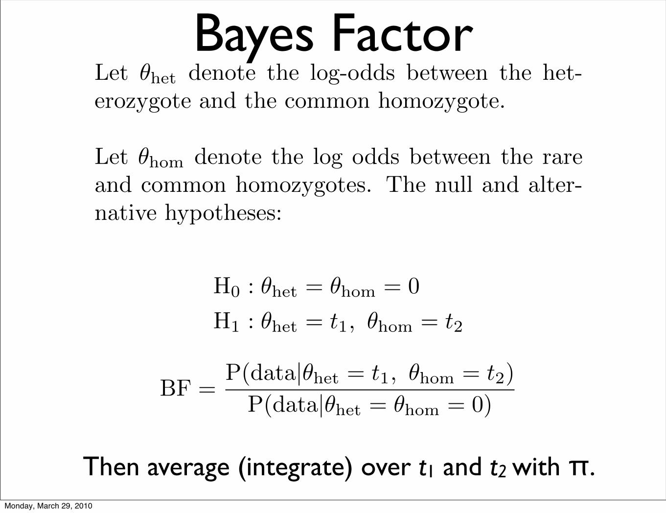
Bayes Factor

Then average (integrate) over t1 and t2 with π.

Let θhet denote the log-odds between the het-

erozygote and the common homozygote.

Let θhom denote the log odds between the rare

and common homozygotes. The null and alter-

native hypotheses:

H0 : θhet = θhom = 0

H1 : θhet = t1, θhom = t2

BF =P(data|θhet = t1, θhom = t2)

P(data|θhet = θhom = 0)


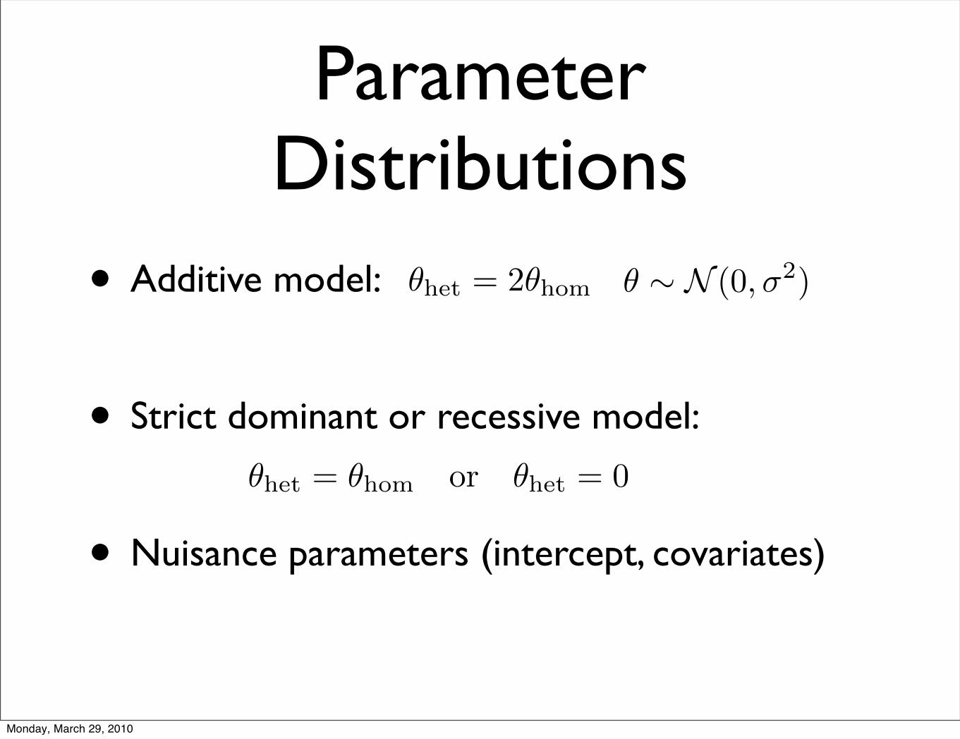
• Additive model:

• Strict dominant or recessive model:

• Nuisance parameters (intercept, covariates)

Parameter Distributions

θhet = 2θhom

θhet = θhom or θhet = 0

θ ∼ N (0,σ2)


Bayesian vs Frequentist on WTCCC Data


Continuous outcomes: linear regression


!

SNP genotype

Phen

otyp

ic s

core

0 1 2

4.5

4.0

3.5

3.0

2.5

2.0

Stepwise selection procedureDescribes a class of statistical procedures that identify from a large set of variables (such as SNPs) a subset that provides a good fit to a chosen statistical model (for example, a regression model that predicts case–control status) by successively including or discarding terms from the model.

Shrinkage methodsIn this approach a prior distribution for regression coefficients is concentrated at zero, so that in the absence of a strong signal of association, the corresponding regression coefficient is ‘shrunk’ to zero. This mitigates the effects of too many variables (degrees of freedom) in the statistical model.

kinship, with or without an explicit subpopulation effect, has recently been found to outperform GC in many set-tings56. Given large numbers of null SNPs, it becomes possible to make precise statements about the (distant) relatedness of individuals in a study so that a complete solution to the problem of population stratification — which has in the past been the cause of much concern — is probably not far away.

Tests of association: multiple SNPsGiven L SNPs genotyped in cases and controls at a candidate gene that is subject to little recombination, or perhaps an LD block within a gene, we might want to decide whether or not the gene is associated with the disease and/or, given that there is association, find the SNP(s) that are closest to the causal polymorphism(s).

Analysing SNPs one at a time can neglect information in their joint distribution. This is of little consequence in the two extreme cases: when SNPs are widely spaced so as to have little or no LD between them or when almost all SNPs are typed so that any causal variant is likely to be typed in the study. In practice, most studies have SNP densities between these two extremes, in which case multipoint association analyses have substantial advan-tages over single-SNP analyses57. I first outline regression analyses of unphased SNP genotypes and then move on to haplotype-based analyses.

SNP-based logistic regression. Logistic regression analyses for L SNPs are a natural extension of the single-SNP anal-yses that are discussed above: there is now a coefficient (!0, !1 or !2) for each SNP, leading to a general test with 2L df. By constraining the coefficients, tests with L df can be obtained. For example, a test for additive effects at each SNP is obtained by requiring that each !1 = (!0 + !2) / 2. The corresponding score test, also with L df, is a generali-zation of the Armitage test, and is related to the Hotelling T2 statistic56. Another test, with L+1 df, uses only 1 df to capture gene-wide dominance effects29.

Covariates such as sex, age or environmental expo-sures are readily included. Similarly, interactions between SNPs can be included. This conveys little benefit, and can reduce power to detect an association, if there is a single underlying causal variant and little or no recombination between SNPs58, but it is potentially useful for investigating epistatic effects.

If the number of SNPs is large, tagging to eliminate near-redundant SNPs often increases power despite some loss of information. Alternatively, the problem of too many highly correlated SNPs in the model can be addressed using a stepwise selection procedure59 or Bayesian shrinkage methods60. However, problems can arise in assessing the significance of any chosen model.

Essentially the same issues arise for a continuous phenotype; the same sets of coefficients are appropriate but they are equated to the expected phenotype value rather than the logit of disease risk.

Haplotype-based methods. The multi-SNP analyses discussed above can suffer from problems that are associated with many predictors, some of which are highly

correlated. A popular strategy, suggested by the block-like structure of the human genome, is to use haplotypes to try to capture the correlation structure of SNPs in regions of little recombination. This approach can lead to analyses with fewer degrees of freedom, but this benefit is minimized when SNPs are ascertained through a tag-ging strategy. Perhaps more importantly, haplotypes can capture the combined effects of tightly linked cis-acting causal variants61.

An immediate problem is that haplotypes are not observed; instead, they must be inferred and it can be hard to account for the uncertainty that arises in phase inference when assessing the overall significance of any finding. However, when LD between markers is high, the level of uncertainty is usually low.

Given haplotype assignments, the simplest analysis involves testing for independence of rows and columns in a 2 ! k contingency table, where k denotes the number of distinct haplotypes62. Alternative approaches can be based on the estimated haplotype proportions among cases and controls, without an explicit haplotype assign-ment for individuals63: the test compares the product of separate multinomial likelihoods for cases and controls with that obtained by combining cases and controls. One problem with both these approaches is reliance on assumptions of HWE and of near-additive disease risk. A different approach, which leads to a test with fewer degrees of freedom, is to look for an excess sharing of haplotypes among cases relative to controls64. More sophisticated haplotype-based analyses treat haplotypes as categorical variables in regression analyses65 or

Figure 3 | Linear regression test of single-SNP associations with continuous outcomes. Values of a quantitative phenotype for three SNP genotypes, together with least-squares regression line. Note that here the line gives a predicted trait value for the rare homozygote (2) that exceeds the observed values, suggesting some deviation away from the assumption of linearity. Analysis of variance (ANOVA) does not require linearity of the trait means, at the cost of one more degree of freedom. Both tests also require the trait variance to be the same for each genotype: the graph is suggestive of decreasing variance with increasing genotype score, but there is not enough data to confirm this, and a mild deviation from this assumption is unlikely to have an important adverse effect on the validity of the test.

R E V I E W S



ANOVA (2 degrees of freedom)

Regression (1 degree of freedom)


Case-Control: Logistic Regression

• logit (π) = log (π / (1 − π))

• β0 = β1 = β2 -- 2 degrees of freedom

• β1 is half-way between β1 and β2 -- one degree of freedom

• recessive or dominant effects: β0 = β1 or β1 = β2

• fast score test implementations


Categorical Outcomes

• Un-ordered outcomes: multinomial regression

• Ordered outcomes (e.g. mild, moderate, severe): ordinal multinomial regression

- proportional odds: the odds of an individual having a disease state in or above a given category is the same for all categories

- adjacent categories regression: risk of category k relative to k−1 is the same for all k


Other Considerations

• population stratification

• multiple SNPs

• epistatic and gene-environment interactions

• multiple testing


Forest Plot


genetic association - pennsylvania state university association monday, march 29, 2010. ... to share...

Documents