Vol. 10(10), pp. 189-202, October 2016

DOI: 10.5897/AJPS2016.1426

Article Number: FD3BBA161075

ISSN 1996-0824

Copyright © 2016

Author(s) retain the copyright of this article

http://www.academicjournals.org/AJPS

African Journal of Plant Science

Full Length Research Paper

Genotype by environment interaction in sesame (Sesamum indicum L.) cultivars in Uganda

Walter Okello-Anyanga1,2*, Patrick Rubaihayo1, Paul Gibson1 and Patrick Okori1

1Department of Agricultural Production, School of Agricultural Sciences, Makerere University, Kampala, P.O. Box.

7062, Kampala, Uganda. 2National Semi-Arid Resources Research Institute (NaSARRI), Serere, P.O. Soroti, Uganda.

Received 10 May, 2016; Accepted 4 August, 2016

Sesame (Sesamum indicum L.) is an important and ancient oilseed crop cultivated in hot, dry climates for its oil and protein rich seeds. On the African continent, Uganda ranks seventh in sesame production. The improvement of new genotypes with the desired yield stability and performance in different environments is an important issue in breeding programs. In order to identify high yielding and stable sesame genotypes across environments, field experiments were conducted with 16 genotypes for four seasons (2011-2013) at three locations, viz. Serere, Kaberamaido and Ngetta. The objective of the study was to use additive main effects and multiplicative interaction (AMMI) and genotype by genotype environment interaction (GGE) biplot statistical analysis to identify the stability and yield potential of sixteen sesame genotypes. The results of AMMI analysis of variance for seed yield (kg/ha) showed that all the sources of variations that included treatments, genotypes, environments, blocks, interactions, IPCA1 and IPCA 2 were highly significant (P<0.001). The combined analysis of variance indicated that season, season x location, genotype and location x genotype had highly significant (P<0.001) variation. The GGE biplot suggested the existence of only one sesame mega-environment with genotype G9 (Local 158-1) best adapted in that mega-environment followed by G1 (Ajimo A1-6//7029)-1-1. The mega-environment had environments K2011B, K2012A, K2012B, N2012B and K2013B. The vertex genotypes which indicated that they were the most responsive in their respective environments were G2 (Ajimo A1-6//7029)-1-9, G3 (Local 158//6022)-1-2-1, G8 (EM15-3-2), G9 (Local 158-1), G12 (Renner 1-3-1-16) and G14 (Renner 1-3-1-17-1). Genotypes G2 and G12 performed poorly in poor environments. Genotypes were categorized into stable and high yielding, stable but poor yielding, unstable but good yielding and unstable and poor yielding. Environment K2013B was the most discriminating environment. According to the ideal-genotype biplot, genotype G9 (Local 158-1) was the best performing genotype and Kaberamaido was the nearest to ideal environment. It was officially released as Sesim 3 variety for commercial production because of its yield, stability, tolerance to pests and high oil content. Key words: Adaptation, additive main effects and multiplicative interaction (AMMI), genotype environment interaction (GGE) biplot, principal component analysis, stability.

INTRODUCTION Sesame (Sesamum indicumL.) belongs to the Pedaliaceae (order Lamiales) with a small family of 15 genera and 70 species characterised by annual and perennial growth forms. Sesame is an important and

ancient oilseed crop cultivated in hot, dry climates for its oil and protein-rich seeds (Bedigian and Harlan, 1986). Currently, sesame is grown throughout the tropical and subtropical regions of the world with Sudan, China, India,

190 Afr. J. Plant Sci. and Myanmar being the top producers in 2014, together covering 46% of the world production (FAOSTAT, 2015). On the African continent, Uganda (124,300 t) ranks seventh in sesame production (FAOSTAT, 2015). Sesame is commonly known as simsim in Uganda and East Africa generally.

It is often referred to by the epithet „‟the queen of oil seeds‟‟ because of its nutritive value, quality and quantity of its oil which is rich in vitamin E and has a significant amount of linoleic acid that can control blood cholestrol levels (Vijayarajan et al., 2007).

It is an important annual oilseed crop in the tropics and warm sub-tropics where it is mainly grown in small plots as source of edible oil and one of the ingredients in food products. The seed is also rich in protein, vitamins including minerals and lignans such as sesamolin and sesamin (Moazzami and Kamal-Eldin, 2006). Sesame oil has medicinal and pharmaceutical value and is being used in many health care products (Coulman et al., 2005). The seed contains 50 to 60% oil and 25% protein with antioxidants lignans such as sesamolin, sesamol, sesamin which impart to it a high degree of resistance against oxidative rancidity and gives it a long shelf life (Ashri, 1989). It has been used as an active ingredient in antiseptics, bactericides, viricides, disinfectants, moth repellants and anti-tubercular agents (Bedigian et al., 1985). It is a source of calcium, tryptophan, methionine and many minerals (Johnson et al., 1979).

Plant variety trials are routinely conducted to compare multiple genotypes in multiple environments (years and locations) for multiple traits, resulting in genotype by environment by trait three-way data (Yan and Tinker, 2006). Variety trials provide essential information for selecting and recommending crop cultivars. However, variety trial data are rarely utilized to their full capacity. Furthermore, analysis of genotype by environment data is often limited to genotype evaluation based on genotype main effect (G) while genotype-by-environment interactions (GE) are treated as noise or a confounding factor. A larger GEI variation usually hinders the accuracy of yield estimation and reduces the correlation between genotypic and phenotypic values.

According to Yan and Kang (2003), it is known that mean yield across environments are sufficient indicator of genotype performance only in the absence of genotype by environment interaction. Most of the time, GEI complicates breeding, testing and selection of superior genotypes. It is important for breeders developing new varieties to identify specific genotypes adapted or stable to different environment(s), thereby achieving quick genetic gain through screening of genotypes for high adaptation and stability under varying environmental conditions prior to their release as cultivars.

In variety selection experimentation, many genotypes are normally tested over a wide range of environments. Plant breeders perform multi-environmental trials (MET) to evaluate new improved genotypes across test environments before a specific genotype is released for production (Rahmatollah et al., 2013). In such experiments, genotype x environment (GE) interaction is commonly evaluated (Yan et al., 2007). GE interaction effects are of special interest for identifying the most stable genotypes, mega-environments and adaptation targets in most plant breeding programs (Sabaghnia et al., 2013).

Some parameters could be used to study the stability such as regression slope (bi), equivalency (Wi

2),

coeefficient of determination (Ri2), Si

2 ), analysis of

variance (ANOVA), principal component analysis (PCA), additive main effects and multiplicative interaction (AMMI) and genotype genotype x envionment (GGE) biplot. Nevertheless, visualization of the test would be much helpful in concluding the results (Susanto et al., 2015). GGE biplot analysis is one appropriate tool to evaluate representation of an environment, genotype stability, and the effect of G x E to the peformance of a genotype (Rahmatollah et al., 2013). GGE biplot analysis provides an easy and comprehensive solution to genotype by environment data analysis, which has been a challenge to plant breeders, geneticists, and agronomists. GGE biplot analysis is a statistical method which used multivariate approach in the analysis. It is better than univariate approach in dissecting GxE components into specific interaction between genotype and environmental components (Flores et al., 1998). GGE biplot is able to show the best genotype with the highest yield in a quadran containing identical locations (Mega-environments), genotype average performance and stability, ideal genotype and ideal location to increase yield, and specific location (Farshadfar and Sadeghi, 2014). In the AMMI biplot, each genotype is represented by a linear line defined by the genotype‟s mean yield and its interaction principal components axis (IPCA) score on the y-axis and mean yield on the x-axis.

Multivariate techniques like the additive main effects and multiplicative interaction (AMMI) procedure with prediction assessment can be a powerful tool in analyzing multilocation trials (Gauch and Zobel, 1988). The AMMI model combines regular analysis of variance (ANOVA) for additive effects with Principal Component Analysis (PCA) for multiplicative structure within the interaction. A modification of the conventional AMMI analysis proposed by Yan et al. (2000) called GGE biplot (genotype and Genotype-Environment Interaction) has been used to study the GE interaction. The GGE analysis groups together the GE interaction multiplication effect

*Corresponding author. E-mail: waltanyanga@hotmail.com.

Author(s) agree that this article remains permanently open access under the terms of the Creative Commons Attribution

License 4.0 International License

and the genotype effect, which is an additive effect in the AMMI analysis, and analyses these effects by principal components.

Understanding the structure and nature of genotype x environment interaction (GEI) is important in plant breeding programs because a significant GEI can seriously impair efforts in selecting superior genotypes relative to new crop introductions and cultivar development programs. Information on the structure and nature of GEI is particularly useful to breeders because it can help determine if there is need to develop cultivars for all environments of interest or if the need is to develop specific cultivars for specific target environments. In Uganda, work on sesame research for G x E has basically been on the use of ANOVA. This is the first time detailed statistical analysis using multivariate techniques like AMMI and GGE has been applied.

The objective of this study was to use multivariate statistical methods of the GGE biplot and AMMI methodologies to identify the stability and adaptability of sixteen sesame genotypes. MATERIALS AND METHODS Experimental sites and planting materials Sixteen genotypes including the local selected breeding lines and introduced accessions (Table 1) selected for better yield potential and other yield characters among genotypes at National Semi-Arid Resources Research Institute (NaSARRI), Serere were evaluated in three locations of Serere (latitude 1°31‟N; longitude 33°27‟E; and altitude 1,139 mean above sea level (masl), Kaberamaido (latitude 1°44‟N; longitude 33°09‟E; altitude 1,080 masl) and Ngetta (latitude 2°17‟N; longitude 32°56‟E; altitude 1,189 masl) for four seasons. These locations are situated in Serere, Kaberamaido and Lira districts representing different farming systems and different tribal setting. The evaluation experiments were done in 2011B, 2012A, 2012B and 2013B seasons. The first rainy season planting starts about mid-March to April and harvested in July, while the second season‟s planting starts about July to September and harvested about October to December depending on the location and onset of rains. The farmers in Kaberamaido district used to grow their sesame during the first rainy season which starts about mid-March. Serere farmers plant sesame in both seasons. Meanwhile, in Lira district where Ngetta is located, sesame was mainly grown during the second season although in the southern part of the district, sesame is planted during the first season. With changes in weather pattern and increasing market, farmers across locations are now growing sesame twice in a year.

Procedure

A randomized complete block design with 3 replications was used across locations and seasons. Each entry was planted in eight 4-m rows, with spacing of 30 cm between rows and continuous sowing within a row. Thinning within the rows was done to approximately 10 cm between plants. Standard recommended practices like insecticides and fungicides were applied where necessary in order to control insect pests and fungal diseases respectively in order to produce good results. The six middle rows were harvested and used as yield per plot and converted to yield in kilograms per hectare.

Okello-Anyanga et al. 191 Statistical analysis The the data for grain yield were pooled to perform the analysis of variance across locations. Since the pooled analysis of variance considers only the main effects, the additive main effect and multiplicative interaction model (AMMI) was computed. Beginning with the ordinary ANOVA procedure for two way analysis of variance, the AMMI analysis first separates additive variance from the multiplicative variance (interaction), and then applied PCA to the interaction, that is, to the residual portion of the ANOVA model to extract a new set of coordinate axes which accounts more effectively for the interaction patterns (Gauch and Zobel, 1988). AMMI analysis was also used to determine stability of the genotypes across locations using the PCA (principal component axis) scores.

To graphically visualize the relationship between environments (locations by seasons) and entries in order to determine the „which won where‟ portion, and to identify mega environment, a GGE biplot (Yan, 2001) analyis was also undertaken using GGE biplot in the Meta analysis of Genstat 14th edition (Payne et al., 2010).

Analysis of variance (ANOVA) for yield was carried out for individual locations, seasons and for combined analysis across locations. Statistical procedures applied were Principal Component Analysis (PCA), additive main and multiplicative interaction (AMMI), genotype and genotype by environment biplot analysis (GGE). For a simple analysis of variance of a randomized complete block design, the model: Yijk = µ + Gi + Ej + GEij + Bij + ɛijk was applied where µ is the mean, Gi is the effect of the ith genotype, Ej is the effect of the jth environment, GEij is the interaction of the ith genotype with the jth environment, Bij is the effect of the kth replication in the jth environment, and ɛijk is the random error.

Genotype-focused scaling was used in visualizing for genotypic comparison, with environment-focused scaling for environmental comparison. The symmetric scaling was preferred in visualizing the “which-won-where” pattern of multi-environment yield trials (MEYTs) data (Yan, 2002). The biplots were constructed using GenStat 14th Edition (Payne et al., 2010).

AMMI and GGE procedures for estimating G x E interaction were used. The combined analysis was performed and the means served as basis for the AMMI analysis, considering the following model: Yij

= µ + Gi + Ej +

n

k 1 λkɣik αjk + ρij + ɛij , Where: Yij is the mean response of genotype i in environment j; µ is the overall mean; Gi is the genotype effect; Ej is the environment effect; GEij is the

multiplicative component (GE interaction effect) modeled by

n

k 1

λkɣikαjk + ρij + ɛij, where λk is the kth singular of the matrix of original interactions GE; ɣik is the element corresponding to the ith genotype on the kth singular vector of the GE matrix column; αjk is the element corresponding to the jth environment on kth singular vector of the GE matrix row; ρij is the noise associated with expression not explained by the principal components; and ɛij is the associated error.

A GGE biplot was constructed by plotting the first principal components against their respective scores for the second principal component (PC2) that results from singular value dimension (SVD) of environment-centred or environment-standardized.

RESULTS Analysis of variance Analysis of variance (ANOVA) across locations and seasons is presented in Table 2. There was highly significant difference (P<0.001) among the four seasons suggesting high variability among seasons. Seasons

192 Afr. J. Plant Sci. Table 1. Genotypes, origin and their major identifiable characteristics.

Code name

Genotype Origin Yield Resistance to Fusarium wilt disease

Resistance to gall midge

Hairiness on capsules

Branching habit

Plant height

Number of capsules per plant

Days to maturity

G1 (Ajimo A1-6//7029)-1-1

A homozygous cross between a selected Ugandan land race (Ajimo A1-6) and a Thai accession (7029)

High Resistant Highly Resistant Hairy High Tall Many >85

G2 (Ajimo A1-6//7029)-1-9

A homozygous cross between a selected Ugandan land race (Ajimo A1-6) and a Thai accession (7029)

Low Susceptible Resistant Hairy less Short Few Less than 75

G3 (Local 158//6022)-1-2-1

A homozygous cross between an Egyptian accession (Local 158) and a Thai accession (6022)

High Resistant Highly resistant Hairy High Tall Many >85

G4 (Sesim2//5181)-2-2-1

A homozygous cross between a released commercial variety (Sesim 2) and a Thai accession (5181)

High Resistant Highly resistant Hairy Medium Tall Many >85

G5 AD-1-1-1 Pureline Ugandan land race Medium Resistant Medium resistant Smooth High Tall Many >85

G6 Adong 4-4 Pureline Ugandan land race Medium Resistant Medium resistant Smooth High Tall Many >85

G7 EM15-1-5 Pureline Ugandan land race Low Resistant Medium resistant Light hairy High Tall Medium >85

G8 EM15-3-2 Pureline Ugandan land race Medium Resistant Medium resistant smooth High Tall Many >85

G9 Local 158-1 Egyptian pureline High Medium resistant Highly resistant Hairy Medium Tall Many >80

G10 Local 158-5 Egyptian pureline High Medium resistant Highly resistant Hairy Medium Tall Many >80

G11 Renner 1-3-1-14 USA pureline Low Resistant Medium resistant smooth Medium Medium Few >80

G12 Renner 1-3-1-16 USA pureline Low Resistant Medium resistant smooth Medium Short Few >80

G13 Renner 1-3-1-17 USA pureline Medium Resistant Medium resistant smooth Medium Medium Medium >80

G14 Renner 1-3-1-17-1 USA pureline High Resistant Medium resistant smooth Medium Medium Medium >80

G15 Sesim 1 Ugandan commercial variety High Resistant Low resistant smooth High Tall Many >85

G16 Sesim 2 Ugandan commercial variety High Resistant Medium resistant smooth High Tall Many >85

contributed 10% of the total sum of squares for variation. Location showed no significant difference suggesting that locations were similar in conditions. Highly significant difference (P<0.001) was recorded for season x location (S x

L). This showed that there was high interaction between the seasons and locations. Season by location contributed highest in the total sum of squares of variation with 45%. Highly significant difference (P<0.001) was recorded for genotypes.

This showed that there were differences in yield performance among the genotypes. Some genotypes were high yielding while others were poor yielding. Genotypes contributed 4% of the total sum of squares due to variation. Season x

Okello-Anyanga et al. 193 Table 2. Combined analysis of variance of yield data of 16 sesame genotypes tested in 3 locations for 4 seasons.

Source of variation D.F S.S M.S F-value p-value %variation

Season(S) 3 4107465 1369155*** 19.12 <0.001 10

Location (L) 2 12899 6449ns 0.09 0.914 0

Season x Location 6 18088342 3014724*** 42.09 <0.001 45

Residual 24 1718873 71620 3.21

Genotype (G) 15 1934120 128941*** 5.77 <0.001 4

Season x Genotype (S x G) 45 1339039 29756ns 1.33 0.083 3.3

Location x Genotype (L x G) 30 1717895 57263*** 2.56 <0.001 4.3

Season x Location x Genotype (S x L x G) 90 3076274 34181** 1.53 0.003 7.7

Residual 360 8042700 22341

Total 575 40037608

ns = Non-significant; Significant: **P<0.01, ***P< 0.001%.

Table 3. Mean yield performance (kg/ha) and ranking of each genotype for each location over four seasons.

Code no. Genotype NaSARRI Rank Kaberamaido Rank Ngetta Rank Overall mean

Overall rank

G1 (Ajimo A1-6//7029)-1-1 416 6 587 2 566 2 523 2

G2 (Ajimo A1-6//7029)-1-9 309 16 234 16 338 16 294 16

G3 (Local 158//6022)-1-2-1 401 9 563 3 501 7 488 4

G4 (Sesim2//5181)-2-2-1 447 2 531 5 536 4 505 3

G5 AD-1-1-1 393 10 490 8 501 7 461 8

G6 Adong 4-4 425 4 508 7 475 10 469 7

G7 EM15-1-5 345 13 481 9 464 12 430 12

G8 EM15-3-2 375 11 470 10 403 15 416 13

G9 Local 158-1 461 1 700 1 532 5 564 1

G10 Local 158-5 420 5 462 12 444 13 442 11

G11 Renner 1-3-1-14 413 7 293 14 428 14 378 14

G12 Renner 1-3-1-16 338 15 287 15 510 6 378 14

G13 Renner 1-3-1-17 408 8 470 10 541 3 473 6

G14 Renner 1-3-1-17-1 359 12 454 13 571 1 461 8

G15 Sesim 1 431 3 525 6 472 11 476 5

G16 Sesim 2 343 14 541 4 481 9 455 10

Cv% 19.7 24.8 24

Prob. 0.218ns 0.001*** 0.38ns

genotype (S x G) did not show any significant difference suggesting that high yielding genotypes performed better in all seasons and low yielding genotypes performed poorly in all seasons. Combined performance analysis across locations The overall mean yield performance across locations over seasons is presented in Table 3. Genotype G9 (Local 158-1) had the best performance at Serere and Kaberamaido and also the best yield of 564 kgha

-1 across

locations followed by G1 (Ajimo A1-6//7029)-1-1 with 523

kgha-1

. G2 (Ajimo A1-6//7029)-1-9 was the poorest yielding genotype in each location and across locations. The other poor yielding genotypes were G11 (Renner 1-3-1-14) and G12 (Renner 1-3-1-16). There were changes in the ranking within the locations and across locations. Highly significance among genotypes was only recorded for Kaberamaido. AMMI and principal component analysis (PCA) AMMI analysis of variance for seed yield of 16 sesame genotypes is presented in Table 4. The results showed

194 Afr. J. Plant Sci.

Table 4. AMMI analysis of variance for seed yield (kg/ha) of 16 sesame genotypes

Source of variation df SS MS F F prob % of variation

Replication 24 1718873 71620 3.21 0.00000***

Treatments 191 30276034 158513 7.10 0.00000***

Genotypes 15 1934120 128941 5.77 0.00000*** 6.5

Environments 11 22208706 2018973 28.19 0.00000*** 73.4

Interactions 165 6133208 37171 1.66 0.00004*** 20.3

IPCA 1 25 2067259 82690 3.70 0.00000*** 33.7

IPCA 2 23 1149880 49995 2.24 0.00108*** 18.7

Residuals 117 2916069 24924 1.12 0.22414ns

Error 360 8042700 22341

Total 575 40037608 69631

Level of significance: ns=non-significant, *** (P< 0.01).

Figure 1. AMMI biplot showing the main and interaction (PC1) effects of both genotypes and location by seasons on sesame grain yield.

that all the sources of variations were highly significant (P<0.001). Environment contributed the highest total variation of sums of squares with 73.4% followed by interactions with 20.3% and genotypes with 6.5%.

The AMMI biplot showing the main and interaction (PC1) effects of both genotypes and environments on sesame grain yield is presented in Figure 1. The grand mean for the genotype and environment is indicated by vertical dotted lines which was about 500 kg/ha. High yielding genotypes were located on the positive side of

the graph. These were: G1 (Ajimo A1-6//7029)-1-1, G3 (Local 158//6022)-1-2-1, G4 (Sesim 2//5181)-2-2-1), G5 (AD-1-1-1), G6 (Adong 4-4), G7 (EM15-1-5), G9 (Local 158-1), G13 (Renner 1-3-1-17), G14 (Renner 1-3-1-17-1), G15 (Sesim 1) and G16 (Sesim 2). Stable and high yielding genotypes were G4 (Sesim 2//5181)-2-2-1), G6 (Adong 4-4), and G13 (Renner 1-3-1-17) as they are near the origin (Laurentin and Montila, 1999). Stable but poor yielding genotypes were G8 (EM15-3-2) and G10 (Local 158-5) as they are near the origin but on the left side of

Plot of Gen & Env IPCA 2 scores versus means

G8

G6

G16

G7

G2G10 G3

G12

G4G1

G11

G13

G15

G9

G5

G14

S2013B

S2012B

N2012A

N2012B

K2012A

K2013B

N2011B

K2011B

K2012B

N2013B

S2011B

S2012A

200 400

-15

600

-10

-5

0

5

300 700 500

Genotype & Environment means

IPCA

sco

res

Plot of Gen & Env IPCA 2 scores versus means

G8

G6

G16

G7

G2G10 G3

G12

G4G1

G11

G13

G15

G9

G5

G14

S2013B

S2012B

N2012A

N2012B

K2012A

K2013B

N2011B

K2011B

K2012B

N2013B

S2011B

S2012A

200 400

-15

600

-10

-5

0

5

300 700 500

Genotype & Environment means

IPCA

sco

res

Okello-Anyanga et al. 195

Figure 2. Polygon view of GGE biplot analysis showing the mega-environments and their respective high yielding genotypes for „which-won-where‟ pattern.

the vertical line of the genotype and environment means. Poor yielding and unstable genotypes were G2 (Ajimo A1-6//7029)-1-9), G11 (Renner 1-3-14) and G12 (Renner 1-3-1-16) as they are far away from the origin and also positioned on the left side of the vertical line for genotype and environment means. The best performing environments (location x season) were N2011B (Ngetta 2011B), S2012A (Serere 2012A), S2012B (Serere 2012B), K2012A (Kaberamaido 2012A), N2013B (Ngetta 2013B), K2012B (Kaberamaido 2012B) and N2012B (Ngetta 2012B). The poor performing environments were S2013B (Serere 2013B), N2012A (Ngetta 2012A), S2011B (Serere 2011B) and K2011B (Kaberamaido 2011B) with less than 500 kg/ha as the genotype and environment grand mean. Genotypes and location per season located near to the origin are considered to be stable.

GGE analyses

Which-won-where

The results of a pattern of “which-won-where” are

presented in Figure 2. Based on the three locations and seasons used in this study, only one mega-environment was identified as all environments were located in one sector. Locations by seasons within mega-environment 1 were Kaberamaido 2011B, 2012A, 2012B, 2013B and Ngetta 2011B and 2013B. For this mega-environment, G9 (Local 158-1) was the most positively responsive as it was at the vertex and therefore was the highest yielder at the vertex.

The polygon view of the GGE biplot showed that all test environments were divided into 6 sectors. Means performance and stability The results of the average environment coordination (AEC) views of the GGE-biplot based on environment-focus scaling for the means performance and stability of genotypes are presented in Figure 3. GGE biplot analysis produced good visual assessment of GGE with PCA1 (47.21%) and PCA2 (14.25%) explaining 61.47% of the total GE sum of squares. The environmental vector bi-plot identified N2011B and N2012B as highly

G8

G6

G7

G15

G1G16

G11

G2

G13

G3

G9

G12

G14

G10

G4

Scatter plot (Total - 61.47%)

G5

K2013B

K2011B

S2013B

N2011B

N2012B

S2011B

S2012AS2012B

N2012A

N2013B

K2012B

K2012A

PC

2 -

14.2

5%

PC1 - 47.21%

Environment scores

Sectors of convex hull

Convex hull

Mega-Environments

Genotype scores

G8

G6

G7

G15

G1G16

G11

G2

G13

G3

G9

G12

G14

G10

G4

Scatter plot (Total - 61.47%)

G5

K2013B

K2011B

S2013B

N2011B

N2012B

S2011B

S2012AS2012B

N2012A

N2013B

K2012B

K2012A

PC

2 -

14.2

5%

PC1 - 47.21%

Environment scores

Sectors of convex hull

Convex hull

Mega-Environments

Genotype scores

196 Afr. J. Plant Sci.

Figure 3. The average environment coordination (AEC) views of the GGE-biplot based on environment focused scaling for the means performance and stability of genotypes.

Figure 4. The environment vector biplot showing environmental differences in discriminating the 16 genotypes for yield at the twelve test environments

G9

G8

G16 G1

G2

G11

G3

G13

G4

G10

G12

G14

G15G5

G6

G7

Ranking biplot (Total - 61.47%)

N2013B

K2012BS2011B

K2013B

S2012B

N2011B

K2011B

S2012A

S2013B

K2012A

N2012B

N2012A

PC1 - 47.21%

PC2

- 14.

25%

AEC

Environment scores

Genotype scores

G9

G8

G16 G1

G2

G11

G3

G13

G4

G10

G12

G14

G15G5

G6

G7

Ranking biplot (Total - 61.47%)

N2013B

K2012BS2011B

K2013B

S2012B

N2011B

K2011B

S2012A

S2013B

K2012A

N2012B

N2012A

PC1 - 47.21%

PC2

- 14.

25%

AEC

Environment scores

Genotype scores

G6

G11G1G16

G15

G8

G14

G5

G13

G3

G9

G7

G4

G2

Scatter plot (Total - 61.47%)

G12

G10

S2013B

K2011B

N2012A

N2011B

S2012AN2013B

N2012B

S2012B

S2011B

K2013B

K2012B

K2012A

PC2

- 14.

25%

PC1 - 47.21%

Vectors

Environment scores

Genotype scores

G6

G11G1G16

G15

G8

G14

G5

G13

G3

G9

G7

G4

G2

Scatter plot (Total - 61.47%)

G12

G10

S2013B

K2011B

N2012A

N2011B

S2012AN2013B

N2012B

S2012B

S2011B

K2013B

K2012B

K2012A

PC2

- 14.

25%

PC1 - 47.21%

Vectors

Environment scores

Genotype scores

Okello-Anyanga et al. 197

Figure 5. GGE-biplot for comparison of the genotypes with the ideal genotype.

discriminating for the genotypes tested, as evidenced by the long environment vectors. The yield and stability were considered simultaneously and the average environment coordinate (AEC) biplot was generated. The highest yielding and stable genotype was G9 followed by G1. G11 was the most stable but one of the poorest yielders. G12 was the most unstable as it had the longest vector. Unlike PC1, genotypic PC2 scores near zero exhibited stable genotypes whereas large PC2 scores discriminated the unstable ones. S2011B, K2011B, K2012A and K2012B were stable environments while N2011B and N2012B were the most unstable environments. K2013B was the most productive environment but most discriminative for genotypes. Discriminant analysis Discriminating vector showing ability of an environment is presented in Figure 4. Kaberamaido during 2013B (K2013B) was the most discriminating and responsive as it had the longest vector from the biplot origin. They are stable environments but not informative as they were not discriminatory. Environments were positively correlated since the cosine angles were less than 90°. K2011B, K2012A, K2012B, S2011B, N2012A, N2013B and all the

seasons at Serere had short vectors. Genotypes G2, G5, G10, G11, G12 and G14 were not located in any environment. They are poor genotypes that did poorly in most environments. Ideal genotype The GGE-biplot for comparisons of the genotypes with the ideal genotype is presented in Figure 5. The genotype G9 followed by genotypes G1 which were closest to the inner most concentric center. Genotypes G3, G4, G5, G6, G7, G13, G14, G15 and G16 were above the grand mean indicated by the vertical line in the centre are considered desirable genotypes because they are within the circles that surround the circle of the virtual ideal genotype. Genotypes G2, G12 and G11 were furthest from the ideal genotype. Ideal environment Comparison of environments to an ideal environment is presented in Figure 6. In this experiment, the ideal environment was also represented by the central concentric circle with an arrow passing through it and it

G5

Comparison biplot (Total - 61.47%)

G3

G1G4G11

G6

G13

G7

G15

G8

G12

G14

G16

G10

G9

G2

K2011B

S2011B

K2013B

S2012A

N2012AK2012B

N2013B

N2011B

N2012B

S2012B

S2013B

K2012A

PC1 - 47.21%

PC2

- 14

.25%

AEC

Environment scores

Genotype scores

G5

Comparison biplot (Total - 61.47%)

G3

G1G4G11

G6

G13

G7

G15

G8

G12

G14

G16

G10

G9

G2

K2011B

S2011B

K2013B

S2012A

N2012AK2012B

N2013B

N2011B

N2012B

S2012B

S2013B

K2012A

PC1 - 47.21%

PC2

- 14

.25%

AEC

Environment scores

Genotype scores

198 Afr. J. Plant Sci.

Figure 6. GGE-biplot for comparison of environments with the ideal environment.

showed that K2013B (Kaberamaido 2013B) was the closest to ideal environment. K2011B, K2012A, K2012B and N2012B were also desirable environments as they were located in the middle parts of the concentric rings towards the ideal environment. Ngetta 2012A, S2012A, N2013B and S2013B were the worst seasons (environments) as they were the furthest from ideal environment which is in the innermost concentric rings. DISCUSSION Analysis of variance Analysis of variance (ANOVA) across locations and seasons recorded highly significant difference (P<0.001) among the four seasons suggesting that there were changes in the conditions of the weather in the different locations in different seasons. Climatic conditions and different soil constituents cause annual variations (Mortazavian et al., 2014). Seasons contributed 10% of the total sum of squares for variation. Location showed no significant difference suggesting that locations were similar in conditions. Rahmatollah et al. (2013) in their study found similar results. Highly significant difference (P<0.001) was recorded for season x location (S x L). This showed that there was high interaction between the seasons and locations. Season by location contributed highest in the total sum of squares of variation with 45%.

Rahmatollah et al. (2013) recorded similar highly significant year x location effect. Highly significant difference (P<0.001) was recorded for genotypes. This showed that there were differences in yield performance among the genotypes. Some genotypes were high yielding while others were poor yielding. Genotypes contributed 4% of the total sum of squares due to variation. Rahmatollah et al. (2013) also recorded similar significant effect for genotypes and attributed that possibly due to changes in genotype characteristics, varying from one genotype to another. Velu and Shunmugavalli (2005) also reported similar highly significant difference among genotypes. Season x genotype (S x G) did not show any significant difference suggesting that high yielding genotypes performed better in all seasons and low yielding genotypes performed poorly in all seasons. Rahmatollah et al. (2013) also recorded no significant effect in genotype by year although they did not use seasons. Location by genotype interaction (L x G) was highly significant (P<0.001) suggesting that genotypes interacted with locations and performed differently thus changing in ranking. Rahmatollah et al. (2013) also recorded significant location by genotype effect .The season x location x genotype (S x L x G) interaction showed highly significant difference (P<0.001) suggesting that there was high interaction among genotypes during the seasons in those different locations. John et al. (2001) also observed the mean squares for genotypes, seasons (environments)

G12

G11G4

Comparison biplot (Total - 61.47%)

G1

G10

G14

G5

G16

G6 G3

G15

G2

G13

G7

G8

G9

N2013BK2011B

N2012AS2011B

N2011B

N2012B

S2012A

S2013B

K2013B

K2012B

K2012A

S2012B

PC1 - 47.21%

PC2

- 14.

25%

AEC

Environment scores

Genotype scores

G12

G11G4

Comparison biplot (Total - 61.47%)

G1

G10

G14

G5

G16

G6 G3

G15

G2

G13

G7

G8

G9

N2013BK2011B

N2012AS2011B

N2011B

N2012B

S2012A

S2013B

K2013B

K2012B

K2012A

S2012B

PC1 - 47.21%

PC2

- 14.

25%

AEC

Environment scores

Genotype scores

and G x E interactions to be highly significant

Partitioning of variance components for environment into predictable (locations) and unpredictable (seasons or year) is very important (Rahmatollah et al., 2013). When GE interaction is due to variation in predictable factors, a plant breeder has the choice of either developing specific genotypes for selected environments or broadly adapted genotypes that can perform well under variable conditions (Dehghani et al., 2006). When GE interaction results from unpredictable sources, a plant breeder needs to develop stable genotypes that perform reasonably well under a range of environmental conditions.

Combined performance analysis across locations The overall mean yield performance across locations over seasons showed that genotype G9 (Local 158-1) had the best yield of 564 kgha followed by G1 (Ajimo A1-6//7029)-1-1 with 523 kgha

-1. G2 (Ajimo A1-6//7029)-1-9

was the poorest yielding genotype across all locations. G2 is an early maturing genotype and susceptible to sesame Fusarium wilt which tends to reduce its yield in some seasons. Normally early or very early varieties do not perform very well. The local selected lines were adaptable to the local conditions as they have withstood selection pressure within the environment over the years. This is also reported by Ashri (1989). Local 158-1 and its other series, and Sesim2//5181 are hairy genotypes as shown in Table 1 and they have been recorded to be tolerant to sesame gall midge that cause flower and capsule damage to sesame thus reducing yield (Ogwal et al., 2003). Sesim 1 and Sesim 2 had already been officially released in Uganda for commercial production in 2001 and 2003 respectively. Local 158-1 was officially released for commercial production as Sesim 3 in 2013 because of its high yield, stability, seed color and hairyness of the stem and capsules that gives it resistance to gall midge insect (Asphondylia sesame). AMMI and principal component analysis (PCA) AMMI analysis of variance for seed yield of 16 sesame genotypes showed that all the sources of variations were highly significant (P<0.001). Environment contributed the highest total variation of sums of squares with 73.4% followed by interactions with 20.3% and genotypes with 6.4%. Laurentin and Montilla (1999) recorded 94% of the AMMI model sum of squares attributed totally to G x E interaction.

The AMMI biplot showing the main and interaction (PC1) effects of both genotypes and environments on sesame grain yield presented in Figure 1 had high yielding genotypes located on the positive side of the graph. Stable and high yielding genotypes were G4

Okello-Anyanga et al. 199 (Sesim 2//5181)-2-2-1), G6 (Adong 4-4), and G13 (Renner 1-3-1-17) as they are near the origin. Stable but poor yielding genotypes were G8 (EM15-3-2) and G10 (Local 158-5) as they are near the origin but on the left side of the vertical line of the genotype and environment means. Poor yielding and unstable genotypes were G2 (Ajimo A1-6//7029)-1-9), G11 ( Renner 1-3-14) and G12 (Renner 1-3-1-16) as they are far away from the origin and also positioned on the left side of the vertical line for genotype and environment means which indicates areas of low yield (Laurentin and Montila, 1999). Genotypes and location per season located near to the origin are considered to be stable (Laurentin and Montila, 1999). Also, genotypes and environments that fall in the same sector interact positively while those falling into opposite sectors interact negatively (Velu and Shunmugavalli, 2005). GGE analyses Which-won-where The results of a pattern of “which-won-where” as presented in Figure 2, based on the three locations and seasons used in this study showed that only one mega-environment was identified as all environments were located in one sector. Mega environments are test environments with different winning genotypes located at the vertex of the polygon and located in different sectors (Gauch et al., 2008). Locations by seasons within mega-environment 1 were Kaberamaido 2011B, 2012A, 2012B, 2013B and Ngetta 2011B and 2013B. For this mega-environment, G9 (Local 158-1) was the most positively responsive as it was at the vertex and therefore was the highest yielder at the vertex. Although other genotypes were located in other sectors, they did not fall in any environment and therefore those sectors were not considered as mega-environments. Yan et al. (2007) suggested that environment markers that fall into a single sector indicate rank-two approximation with a single cultivar having the highest yield in all environments. If environment markers fall into different sectors, then different cultivars won in different sectors. Since a mega-environment is defined as a group of locations that consistently share the best set of genotypes (Yan and Rajcan, 2002), data from multiple years are essential to decide whether or not the target region can be divided into different mega-environments. Each sector has its most favourable genotypes and corner genotypes not in the environments are the poorest yielding (Karimizadeh, 2013; Pourdad and Moghaddam, 2013). They are located far away from all test locations, reflecting the fact that they yielded poorly at each location.

The polygon view of the GGE biplot showed that all test environments were divided into 6 sectors. Visualization of which-won-where pattern of MEYTs data is important for

200 Afr. J. Plant Sci. studying the possible existence of different mega-environment in a region (Yan and Rajcan, 2002). Corner genotypes which are at the vertex located at the extreme point of the polygon in a sector are the most responsive ones (Rahmatollah et al., 2013). They are the best or the poorest as they are farthest from the origin of the biplot (Yang and Kang, 2003). The polygon view of a GGE biplot explicitly displays the which-won-where pattern (Yan et al., 2001) because each sector would show the vertex with the the indicative genotype and the positions of all other genotypes showing their responsiveness to the environment under study. Genotypes within the polygon are less responsive to location than the vertex genotypes (Rahmatollah et al., 2013).

Mean performance and stability The results of the average environment coordination (AEC) views of the GGE-biplot based on environment-focus scaling for the means performance and stability of genotypes presented in Figure 3 produced good visual assessment of GGE with PCA1 (47.21%) and PCA2 (14.25%) explaining 68.47% of the total GE sum of squares. Farshadfar et al. (2012) partitioned GE interaction through GGE biplot analysis and showed that PC1 and PC2 accounted for 39.1 and 37.79% of GGE sum of squares, respectively, explaining a total of 76.8% variation. The yield and stability were considered simultaneously and the average environment coordinate (AEC) biplot was generated. The average environment, represented by a small circle, was defined by the PC1 and PC2 scores of the environments (Yan and Kang, 2003). The ordinate of the AEC is the line that passes through the origin and is perpendicular to the abscissa. The genotypes G9 (Local 158-1) was the top yielding genotype, as presented on the front of an average environment towards the pointing arrow of the AEC abscissa. In addition, the biplot indicated that G9 had the highest mean yield and one of the most stable genotypes as it was positioned close to the AEC abscissa (Yan, 2002). The second highest yielding and most stable genotype was G1. G12 was the most unstable as it had the longest vector to the AEC. Farshadfar and Sadeghi (2014) explained that genotypic PC1 scores>0 classified the high yielding genotypes while PC1< 0 identified low yielding genotypes. The genotypes with PC1 scores close to zero expressed general adaptation whereas the larger scores depicted more specific adaptation to environments with PC1 scores of the same sign (Ebdon and Gauch, 2002). Unlike PC1, genotypic PC2 scores near zero exhibited stable genotypes whereas large PC2 scores discriminated the unstable ones. S2011B, K2011B, K2012A and K2012B were stable environments while N2011B and N2012B were the most unstable environments. K2013B was the most productive but responsive suggesting that it is high yielding in particular

environment and not stable across environments. The smaller the absolute length of projection of a genotype, the more stable it is (Yan, 2002). A longer projection to the AEC ordinate, regardless of the direction, represent a greater tendency of the GEI of a genotype, which means it is more variable and less stable across environments or vice versa. However, considering both mean yield and stability concepts, plant breeders explore genotypes that indicate yield stability as well as high yield across environments (Kang, 2002). Discriminant analysis Discriminating vector showing ability of an environment presented in Figure 4 showed that location vectors are lines that connect the biplot origin and the marker of test locations. A long environment vector represents good discriminating ability for a given environment (Yan et al., 2000). The lines of the GGE biplot in which the environments are connected with the biplot origin are called vectors. The cosine of the angle between the vectors of two environments is approximate to the correlation coefficient between them (Kroonenberg, 1995; Yan, 2002). The angles between vectors are related to the correlation coefficient (Kroonenberg, 1995). The angles between the environments were less than 90° indicating that most environments were positively correlated to each other. K2013B had the longest vector from the origin and therefore it is highly discriminating for the genotypes tested. Another interesting observation from the vector view of the biplot is that the length of the environment vectors is approximate to the standard deviation within each environment, which is a measure of their discriminating ability (Yan et al., 2003). Long vectors are least stable and those with short vectors and near the horizontal axis are most stable. Ideal genotype The GGE-biplot for comparisons of the genotypes with the ideal genotype presented in Figure 5 showed that the center of the concentric circles is where an ideal genotype (high mean yield and the most stable one) should be located (Yan, 2002). In other words, projection of the ideal genotype on the ATC horizontal axis is equal to the longest vector of all genotypes and its projection on the ATC vertical axis is obviously zero (it is absolutely stable(Yan et al., 2003)). The smaller the distance from genotype to the virtual ideal genotype, the better yielding the genotype. Therefore genotype G9 followed by genotypes G1 which were closest to the concentric center which indicates ideal genotype were the most yielding and stable genotypes. Genotypes G3, G4, G5, G6, G7, G13, G14, G15 and G16 are considered desirable genotypes because they are within the circles

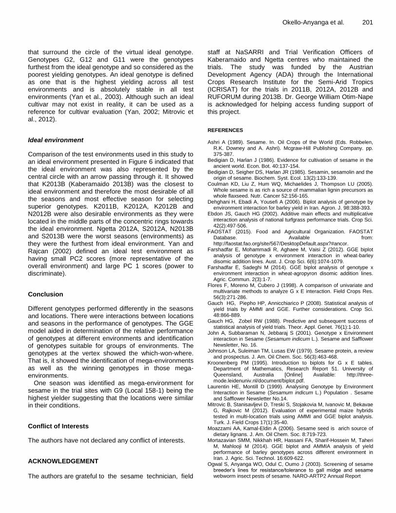
that surround the circle of the virtual ideal genotype. Genotypes G2, G12 and G11 were the genotypes furthest from the ideal genotype and so considered as the poorest yielding genotypes. An ideal genotype is defined as one that is the highest yielding across all test environments and is absolutely stable in all test environments (Yan et al., 2003). Although such an ideal cultivar may not exist in reality, it can be used as a reference for cultivar evaluation (Yan, 2002; Mitrovic et al., 2012).

Ideal environment

Comparison of the test environments used in this study to an ideal environment presented in Figure 6 indicated that the ideal environment was also represented by the central circle with an arrow passing through it. It showed that K2013B (Kaberamaido 2013B) was the closest to ideal environment and therefore the most desirable of all the seasons and most effective season for selecting superior genotypes. K2011B, K2012A, K2012B and N2012B were also desirable environments as they were located in the middle parts of the concentric rings towards the ideal environment. Ngetta 2012A, S2012A, N2013B and S2013B were the worst seasons (environments) as they were the furthest from ideal environment. Yan and Rajcan (2002) defined an ideal test environment as having small PC2 scores (more representative of the overall environment) and large PC 1 scores (power to discriminate).

Conclusion

Different genotypes performed differently in the seasons and locations. There were interactions between locations and seasons in the performance of genotypes. The GGE model aided in determination of the relative performance of genotypes at different environments and identification of genotypes suitable for groups of environments. The genotypes at the vertex showed the which-won-where. That is, it showed the identification of mega-environments as well as the winning genotypes in those mega-environments.

One season was identified as mega-environment for sesame in the trial sites with G9 (Local 158-1) being the highest yielder suggesting that the locations were similar in their conditions.

Conflict of Interests

The authors have not declared any conflict of interests.

ACKNOWLEDGEMENT The authors are grateful to the sesame technician, field

Okello-Anyanga et al. 201 staff at NaSARRI and Trial Verification Officers of Kaberamaido and Ngetta centres who maintained the trials. The study was funded by the Austrian Development Agency (ADA) through the International Crops Research Institute for the Semi-Arid Tropics (ICRISAT) for the trials in 2011B, 2012A, 2012B and RUFORUM during 2013B. Dr. George William Otim-Nape is acknowledged for helping access funding support of this project. REFERENCES Ashri A (1989). Sesame. In. Oil Crops of the World (Eds. Robbelen,

R.K. Downey and A. Ashri). Mcgraw-Hill Publishing Company. pp. 375-387.

Bedigian D, Harlan J (1986). Evidence for cultivation of sesame in the ancient world. Econ. Bot. 40:137-154.

Bedigian D, Seigher DS, Harlan JR (1985). Sesamin, sesamolin and the origin of sesame. Biochem. Syst. Ecol. 13(2):133-139.

Coulman KD, Liu Z, Hum WQ, Michaelides J, Thompson LU (2005). Whole sesame is as rich a source of mammalian lignin precursors as whole flaxseed. Nutr. Cancer 52:156-165.

Dehghani H, Ebadi A, Yousefi A (2006). Biplot analysis of genotype by environment interaction for barley yield in Iran. Agron. J. 98:388-393.

Ebdon JS, Gauch HG (2002). Additive main effects and multiplicative interaction analysis of national turfgrass performance trials. Crop Sci. 42(2):497-506.

FAOSTAT (2015). Food and Agricultural Organization. FAOSTAT Database. Available from: http://faostat.fao.org/site/567/DesktopDefault.aspx?#ancor.

Farshadfar E, Mohammadi R, Aghaee M, Vaisi Z (2012). GGE biplot analysis of genotype x environment interaction in wheat-barley disomic addition lines. Aust. J. Crop Sci. 6(6):1074-1079.

Farshadfar E, Sadeghi M (2014). GGE biplot analysis of genotype x environment interaction in wheat-agropyron disomic addition lines. Agric. Commun. 2(3):1-7.

Flores F, Moreno M, Cubero J (1998). A comparison of univariate and multivariate methods to analyze G x E interaction. Field Crops Res. 56(3):271-286.

Gauch HG, Piepho HP, Annicchiarico P (2008). Statistical analysis of yield trials by AMMI and GGE. Further considerations. Crop Sci. 48:866-889.

Gauch HG, Zobel RW (1988). Predictive and subsequent success of statistical analysis of yield trials. Theor. Appl. Genet. 76(1):1-10.

John A, Subbaraman N, Jebbaraj S (2001). Genotype x Environment interaction in Sesame (Sesamum indicum L.). Sesame and Safflower Newsletter, No. 16.

Johnson LA, Suleiman TM, Lusas EW (1979). Sesame protein, a review and prospectus. J. Am. Oil Chem. Soc. 56(3):463-468.

Kroonenberg PM (1995). Introduction to biplots for G x E tables. Department of Mathematics, Research Report 51. University of Queensland, Australia [Online] Available: http://three-mode.leidenuniv.nl/document/biplot.pdf.

Laurentin HE, Montill D (1999). Analysing Genotype by Environment Interaction in Sesame (Sesamum indicum L.) Population . Sesame and Safflower Newsletter No.14.

Mitrovic B, Stanisavljevi D, Treski S, Stojakovia M, Ivanovic M, Bekavae G, Rajkovic M (2012). Evaluation of experimental maize hybrids tested in multi-location trials using AMMI and GGE biplot analysis. Turk. J. Field Crops 17(1):35-40.

Moazzami AA, Kamal-Eldin A (2006). Sesame seed is arich source of dietary lignans. J. Am. Oil Chem. Soc. 8:719-723.

Mortazavian SMM, Nikkhah HR, Hassani FA, Sharif-Hossein M, Taheri M, Mahlooji M (2014). GGE biplot and AMMIA analysis of yield performance of barley genotypes across different environment in Iran. J. Agric. Sci. Technol. 16:609-622.

Ogwal S, Anyanga WO, Odul C, Oumo J (2003). Screening of sesame breeder‟s lines for resistance/tolerance to gall midge and sesame webworm insect pests of sesame. NARO-ARTP2 Annual Report

202 Afr. J. Plant Sci.

2002-2003. National Agricultural Research Organisation, Ministry of Agriculture, Animal Industry and Fisheries, Entebbe, Uganda.

Payne RW, Harding SH, Murray, DA, Soutar DM, Baird DB, Glaser AR, Thompson R, Webster R (2010). The Guide to Genstat Release 14, Part 2: Statistics. Hemel Hempstead: VSN International, U.K.

Pourdad SS, Moghaddam MJ ( 2013). Study on seed yield stability of sunflower inbred lines through GGE Biplot. Helia 36(58):19-28.

Rahmatollah K, Mohtasham M, Naser S, Ali AM, Barzo R, Faramarz SM, Fariba A (2013). GGE Biplot analysis of yield stability in multienvironment trials of lentil genotypes under rainfed condition. Not. Sci. Biol. 5(2):256-262.

Sabaghnia N, Mohammadi M, Karimizadeh R (2013). Parameters of AMMI Model for Yield Stability Analysis in Durum Wheat. Agric. Conspec. Sci. 78(2):119-124.

Susanto U, Rohaeni WR, Johnson SB, Jamil A (2015). Gge Biplot Analysis For Genotype X Environment Interaction On Yield Trait Of High Fe Content Rice Genotypes In Indonesian Irrigated Environments. Agrivita 37(3):265-275.

Velu G, Shunmugavalli N (2005). Genotype x Environment interaction in sesame (Sesamum indicum L.). Sesame and Safflower Newsletter No. 20.

Vijayarajan S, Ganesh SK, Gunasekaran M (2007). Generation mean analysis for quantitative traits in sesame (Sesamum indicum) crosses. Genet. Mol. Biol. 30(1):80-84.

Yan W (2001). GGE biplot- A windows application for graphical analysis

of multi-environment trial data and other types of two-way data. Agron. J. 93:1111-1118.

Yan W (2002). Singular-value partitioning in biplot analysis of multi-environment trial data. Agron. J. 94:990-996.

Yan W, Cornelius PL, Crossa J, Hunt LA (2001). Two types of GGE biplots for analyzing multi-environment trial data. Crop Sci. 41:656-663.

Yan W, Hunt LA, Sheng Q, Szlavnics Z (2000). Cultivar evaluation and mega-environment investigation based on the GGE biplot. Crop Sci. 40:597-605.

Yan W, Kang MS (2003). GGE biplot analysis: A graphical tool for breeders, geneticists and agronomists. CRC press, Boca Ratoon, Florida.

Yan W, Kang MS, Ma B, Woods S, Cornelius PL (2007). GGE biplot vs AMMI analysis of genotype-by-environment data. Crop Sci. 47:643-655.

Yan W, Rajcan I (2002). Bi-plot Analysis of Test Sites and Trait Relations of Soybean in Ontario. Crop Sci. 42:11-20.

Yan W, Tinker NA (2006). Biplot analysis of multi-environment trial data. Principles and applications. Can. J. Plant Sci. 86(3):623-645.