geocentrix repute 2 2.5 reference manual… · 2 geocentrix repute 2.5 reference manual ... the...
TRANSCRIPT
Geocentrix
Repute 2.5Reference Manual
Onshore pile design and analysis
2 Geocentrix Repute 2.5 Reference Manual
Information in this document is subject to change without notice and does not representa commitment on the part of Geocentrix Ltd. The software described in this document isfurnished under a licence agreement or non-disclosure agreement and may be used orcopied only in accordance with the terms of that agreement. It is against the law to copythe software except as specifically allowed in the licence or non-disclosure agreement. Nopart of this manual may be reproduced or transmitted in any form or by any means,electronic or mechanical, including photocopying and recording, for any purpose, withoutthe express written permission of Geocentrix Ltd.
©2002-17 Geocentrix Ltd. All rights reserved.
"Geocentrix" and "Repute" are registered trademarks of Geocentrix Ltd. Other brand orproduct names are trademarks or registered trademarks of their respective holders
PGroupN is used under exclusive licence from Geomarc Ltd. PGROUP code used underlicence from TRL Ltd.
Set in Optimum using Corel® WordPerfect® X7. Printed in the UK.
Acknowledgments
Repute 2.0 was developed with the generous support of Corus, Atkins, and StentFoundations.
Repute was designed and written by Dr Andrew Bond of Geocentrix, with assistance fromIan Spencer of Honor Oak Systems.
PGroupN was designed and written by Dr Francesco Basile of Geomarc. Special recognitiongoes to the late Dr Ken Fleming of Cementation Foundations Skanska for his invaluableadvice and support during the development of PGroupN.
The Repute Reference Manual was written by Andrew Bond and Francesco Basile.
The following people and organizations assisted with the production of the program and itsdocumentation: Francesco Basile, Jenny Bond, Joe Bond, Tom Bond, Jack Offord, and ClaireBond.
Revision history
Last revised 18th August 2017 (for version 2.5.1).
Table of contents 3
Table of contents
Acknowledgments 2Revision history 2Table of contents 3
Chapter 1Documentation. . . . . . . . . . . . . . . . . . . . . . . . . . . . . . . . . . . . . . . . . . . . . . . . . . . . . . 5
Chapter 2Calculations. . . . . . . . . . . . . . . . . . . . . . . . . . . . . . . . . . . . . . . . . . . . . . . . . . . . . . . . 6
Boundary element analysis 6Fleming’s analysis 15Longitudinal ULS 16Randolph’s analysis 17Validation 18
Chapter 3Design standards. . . . . . . . . . . . . . . . . . . . . . . . . . . . . . . . . . . . . . . . . . . . . . . . . . . 20
Partial (safety) factors 20
Chapter 4Actions.. . . . . . . . . . . . . . . . . . . . . . . . . . . . . . . . . . . . . . . . . . . . . . . . . . . . . . . . . . . 23
Sign convention 23Combinations of actions 24Forces 25Moments 25
Chapter 5Material and section properties. . . . . . . . . . . . . . . . . . . . . . . . . . . . . . . . . . . . . . . . 26
Soils 26Concretes 35Steels 36Bearing piles 36Circular section 37Custom section 37Rectangular section 37
Chapter 6Algorithms.. . . . . . . . . . . . . . . . . . . . . . . . . . . . . . . . . . . . . . . . . . . . . . . . . . . . . . . . 38
Alpha algorithm 38Bearing capacity algorithm 39Bearing pressure limit 41Beta algorithm 41Lateral earth pressure coefficient 41
4 Geocentrix Repute 2.5 Reference Manual
Plugging algorithm 42Shrinkage algorithm 42Skin friction limit 43
43
Chapter 7References. . . . . . . . . . . . . . . . . . . . . . . . . . . . . . . . . . . . . . . . . . . . . . . . . . . . . . . . . 45
Documentation 5
Chapter 1Documentation
Repute is supplied with a detailed Quick-Start Guide, comprehensive User Manual, andauthoritative Reference Manual. The latest versions of these manuals (including anycorrections and/or additions since the program’s first release) are available in electronic(Adobe® Acrobat®) format from the Geocentrix website. Please visitwww.geocentrix.co.uk/repute and follow the links to Repute’s documentation.
Quick-Start guide
The Repute Quick-Start Guide includes six tutorials that show you how to use the mainfeatures of Repute. Each tutorial provides step-by-step instructions on how to drive theprogram. There are three tutorials dealing with single pile design and three with pile groupdesign. The tutorials increase in difficulty and are designed to be followed in order.
User manual
The Repute User Manual explains how to use Repute. It provides a detailed description ofthe program’s user interface, which is being rolled out across all of Geocentrix’s softwareapplications. The manual assumes you have a working knowledge of Microsoft Windows,but otherwise provides detailed instructions for getting the most out of Repute.
Reference manual (this book)
The Repute Reference Manual gives detailed information about the engineering theory thatunderpins Repute’s calculations. The manual assumes you have a working knowledge of thegeotechnical design of single piles and pile groups, but provides appropriate references forfurther study if you do not.
6 Geocentrix Repute 2.5 Reference Manual
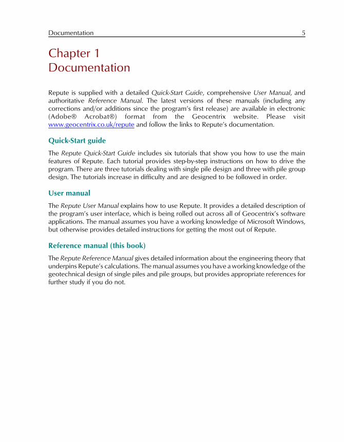
Figure 1. Plan view of a 2 x 2 pile groupin the XY plane
Chapter 2Calculations
Repute® provides a variety of calculations that you can perform on single-piles and pile-groups:
! ”Boundary element analysis” predicts the load vs displacement behaviour of a singlepile or pile group under vertical, horizontal, and moment loading
! ”Fleming’s analysis” predicts the load vs settlement behaviour of a single pile
! ”Longitudinal ULS” checks the ultimate limit state of a single pile under verticalloading
! ”Randolph’s analysis” predicts the settlement of a single pile
! ”Validation” checks single piles and pile groups are properly specified
Boundary element analysis
Repute’s boundary element analysis predicts the load vs displacement behaviour of a singlepile or pile group using the calculation engine PGroupN, developed by Dr Francesco Basileof Geomarc. PGroupN provides a complete 3D non-linear boundary element solution of thesoil continuum, i.e. the simultaneous influence of all the pile elements within the group isconsidered. This overcomes limitations of traditional interaction-factor methods and givesmore realistic predictions of deformations and the load distribution between piles.
The PGroupN program is based on a completeboundary element (BEM) formulation, extendingan idea first proposed by Butterfield andBanerjee [1] and then developed by Basile [2],[3], [4]. The method employs a substructuringtechnique in which the piles and the surroundingsoil are considered separately and thencompatibility and equilibrium conditions areimposed at the interface. Given unit boundaryconditions, i.e. pile group loads and moments,these equations are solved, thereby leading tothe distribution of stresses, loads and moments inthe piles for any loading condition.
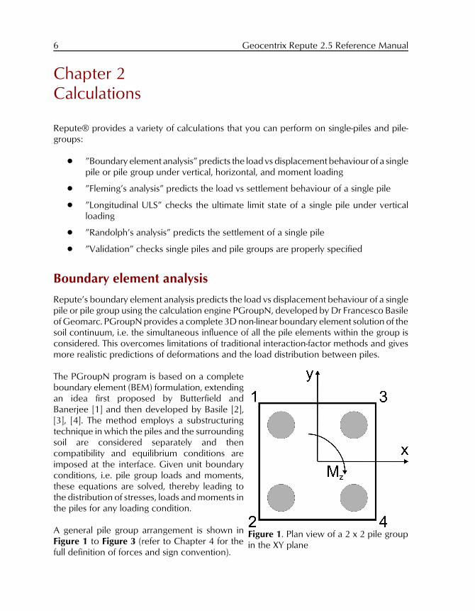
A general pile group arrangement is shown inFigure 1 to Figure 3 (refer to Chapter 4 for thefull definition of forces and sign convention).
Calculations 7
Figure 2. Profile of a 2 x 2 pile group in the XZ plane
Modelling the pile-soil interface (interface discretization)
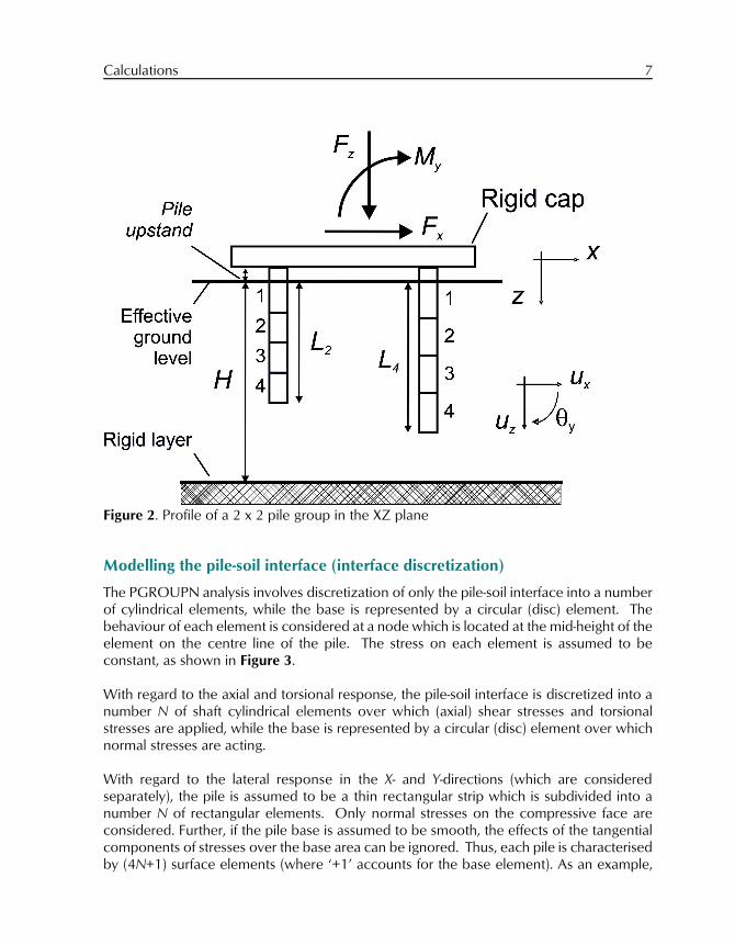
The PGROUPN analysis involves discretization of only the pile-soil interface into a numberof cylindrical elements, while the base is represented by a circular (disc) element. Thebehaviour of each element is considered at a node which is located at the mid-height of theelement on the centre line of the pile. The stress on each element is assumed to beconstant, as shown in Figure 3.
With regard to the axial and torsional response, the pile-soil interface is discretized into anumber N of shaft cylindrical elements over which (axial) shear stresses and torsionalstresses are applied, while the base is represented by a circular (disc) element over whichnormal stresses are acting.
With regard to the lateral response in the X- and Y-directions (which are consideredseparately), the pile is assumed to be a thin rectangular strip which is subdivided into anumber N of rectangular elements. Only normal stresses on the compressive face areconsidered. Further, if the pile base is assumed to be smooth, the effects of the tangentialcomponents of stresses over the base area can be ignored. Thus, each pile is characterisedby (4N+1) surface elements (where ‘+1’ accounts for the base element). As an example,
8 Geocentrix Repute 2.5 Reference Manual
Figure 3. Discretization of the pile-soil interface into N = 6shaft elements
with reference to the pile-soil interface discretization into N = 6 elements illustrated inFigure 3, the vector of soil tractions (ts) has a dimension equal to 25 (i.e. six components forthe axial soil tractions on the shaft plus one axial component on the base, six componentsfor the transverse soil tractions in the X-direction, six components for the transverse soiltractions in the Y-direction, and six components for the torsional soil tractions in the XYplane).
Modelling the soil (soildomain)
The boundary elementmethod involves theintegration of an appropriateelementary singular solutionfor the soil medium over thesurface of the problemdomain, i.e. the pile-soilinterface. With reference tothe present problem whichinvolves an unloadedground surface, thewell-established solution ofMindlin [5] for a point loadwithin a homogeneous,isotropic elastic half spacehas been adopted. The soildeformations at the pile-soilinterface are related to thesoil tractions via integrationof the Mindlin's kernel,yielding:
where {us} are the soildisplacements, {ts} are thesoil tractions and [Gs] is af lex ib i l i ty mat r ix o fcoefficients obtained fromMindlin's solution for theaxial and lateral response.
The off-diagonal flexibilitycoefficients are evaluated by approximating the influence of the continuously distributedloads by discrete point loads applied at the location of the nodes. The singular part of thediagonal terms of the [Gs] matrix is calculated via analytical integration of the Mindlinfunctions. This is a significant advance over previous work (e.g. PGROUP) where these have
Calculations 9
been integrated numerically, since these singular integrals require considerable computingresources. Further computational efficiency is achieved by exploiting symmetries andsimilarities in forming single-pile and interaction flexibility matrices. This reduces thecomputational time and renders the analysis practical for large groups of piles.
Treatment of Gibson and multi-layered soil profiles
Mindlin's solution is strictly applicable to homogeneous soil conditions. However, inpractice, this limitation is not strictly adhered to, and the influence of soil non-homogeneityis often approximated using some averaging of the soil moduli. PGroupN handles Gibsonsoils (i.e. soils whose stiffness increases linearly with depth) and generally multi-layered soilsaccording to an averaging procedure first examined by Poulos [6] and widely accepted inpractice [7], [8], [9], [10], [11], i.e. in the evaluation of the influence of one loaded elementon another, the value of soil modulus is taken as the mean of the values at the twoelements.
Poulos’s procedure is adequate in most practical cases but becomes less accurate if largedifferences in soil modulus exist between adjacent elements or if a soil layer is overlain bya much stiffer layer (Poulos [12]). In such cases, the alternative procedure proposed byYamashita et al. [13] may be adopted for the axial response analysis. For the genericelement i, this procedure calculates an equivalent value of soil modulus on the basis ofweighted average values of soil modulus over 4 elements above and 4 elements below theelement i. At the pile top, the averaging process is curtailed so as not to include non-existentelements. At the pile base, in order to consider the influence of soil layers below the pile tip,the equivalent value also takes into account the values of soil modulus down to a depthequal to the height of 4 ‘imaginary’ elements below the pile base (Note: these elements aretermed ‘imaginary’ because only the pile-soil interface is discretised into elements, i.e. thereare no ‘real’ elements below the pile base.)
It should be pointed out that the Poulos averaging procedure does not consider theinfluence of soil layers located below pile tip.
Rigid layer
Mindlin's solution has been used to obtain approximate solutions for a layer of finitethickness by employing the Steinbrenner approximation [14] to allow for the effect of anunderlying rigid layer in reducing the soil displacements (Poulos [12]; Poulos and Davis[15]). If a rigid layer is defined, it must be the last (i.e. bottom) layer. It is assumed that therigid layer, which is considered to be semi-infinite in extent, cannot be located higher than110% of the embedded length of the longest pile in the group.
Modelling the piles (pile domain)
If the piles are assumed to act as simple beam-columns which are fixed at their heads to thepile cap, the displacements and tractions over each element can be related to each othervia the elementary beam theory, yielding:
10 Geocentrix Repute 2.5 Reference Manual
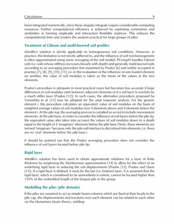
where {up} are the pile displacements, {tp} are the pile tractions, {B} are the piledisplacements due to unit boundary displacements and rotations of the pile cap, and [Gp]is a matrix of coefficients obtained from the elementary (Bernoulli-Euler) beam theory.
Solution of the system
Applying the previous two equations via compatibility and equilibrium constraints at thepile-soil interface, leads to the following system of equations:
where [Gp + Gs] is the global square matrix of the pile group.
By successively applying unit boundary conditions, i.e. unit vertical displacement, unithorizontal displacements (in the X- and Y-directions) and unit rotations (in the XZ, YZ, andXY planes) to the pile cap, it is possible to obtain the system of vertical loads, horizontalloads (in the X- and Y-directions) and moments (in the XZ, YZ, and XY planes) acting on thecap that are necessary to equilibrate the stresses developed in the piles.
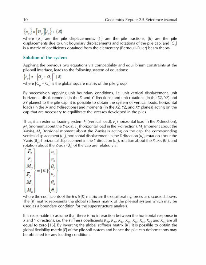
Thus, if an external loading system Fz (vertical load), Fx (horizontal load in the X-direction),My (moment about the Y-axis), Fy (horizontal load in the Y-direction), Mx (moment about theX-axis), Mz (torsional moment about the Z-axis) is acting on the cap, the correspondingvertical displacement (uz), horizontal displacement in the X-direction (ux), rotation about theY-axis (2y), horizontal displacement in the Y-direction (uy), rotation about the X-axis (2x), androtation about the Z-axis (2z) of the cap are related via:
where the coefficients of the 6 x 6 [K] matrix are the equilibrating forces as discussed above.The [K] matrix represents the global stiffness matrix of the pile-soil system which may beused as a boundary condition for the superstructure analysis.
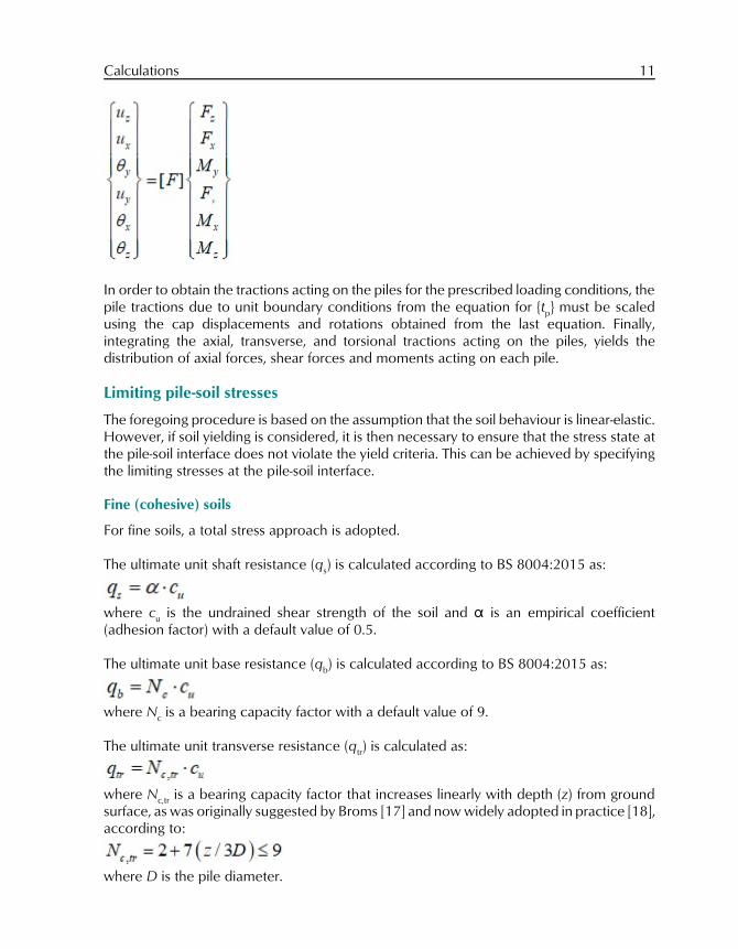
It is reasonable to assume that there is no interaction between the horizontal response inX and Y directions, i.e. the stiffness coefficients K24, K25, K34, K35, K42, K43, K52 and K53 are allequal to zero [16]. By inverting the global stiffness matrix [K], it is possible to obtain theglobal flexibility matrix [F] of the pile-soil system and hence the pile cap deformations maybe obtained for any loading condition:
Calculations 11
In order to obtain the tractions acting on the piles for the prescribed loading conditions, thepile tractions due to unit boundary conditions from the equation for {tp} must be scaledusing the cap displacements and rotations obtained from the last equation. Finally,integrating the axial, transverse, and torsional tractions acting on the piles, yields thedistribution of axial forces, shear forces and moments acting on each pile.
Limiting pile-soil stresses
The foregoing procedure is based on the assumption that the soil behaviour is linear-elastic.However, if soil yielding is considered, it is then necessary to ensure that the stress state atthe pile-soil interface does not violate the yield criteria. This can be achieved by specifyingthe limiting stresses at the pile-soil interface.
Fine (cohesive) soils
For fine soils, a total stress approach is adopted.
The ultimate unit shaft resistance (qs) is calculated according to BS 8004:2015 as:
where cu is the undrained shear strength of the soil and " is an empirical coefficient(adhesion factor) with a default value of 0.5.
The ultimate unit base resistance (qb) is calculated according to BS 8004:2015 as:
where Nc is a bearing capacity factor with a default value of 9.
The ultimate unit transverse resistance (qtr) is calculated as:
where Nc,tr is a bearing capacity factor that increases linearly with depth (z) from groundsurface, as was originally suggested by Broms [17] and now widely adopted in practice [18],according to:
where D is the pile diameter.
12 Geocentrix Repute 2.5 Reference Manual
Coarse (cohesionless) soils
For coarse soils, an effective stress approach is adopted.
The ultimate unit shaft resistance (qs) is calculated according to BS 8004:2015 as:
where Ks is the coefficient of horizontal soil stress, * the angle of friction between pile andsoil, and FNv the vertical effective stress in the free field.
The ultimate unit base resistance (qb) is calculated according to BS 8004:2015 as:
where Nq is a bearing capacity factor that depends on the soil’s angle of shearing resistance(n), By default, Nq is calculated using the equation established by Berezantzev et al. [19] andapproximated in Fleming et al. [57] by:
where n is entered in degrees.
The ultimate unit transverse resistance (qtr) is calculated according to Fleming et al. [57] as:
where Kp is the passive earth pressure coefficient.
Rocks
For rocks, an approach based on unconfined compressive strength is adopted.
The ultimate unit shaft resistance (qs) is calculated according to BS 8004:2015 as:
where qu is the unconfined compressive strength of the intact rock; pa is atmosphericpressure (100 kPa); and k1 and k2 are constants. With the default values k1 = 0.79 and k2 =0.5, this equation reproduces that proposed by Poulos and Bunce [20] (with qs and qu inMPa):
The ultimate unit base resistance (qb) is calculated according to BS 8004:2015 as:
where k3 and k4 are constants (with default values k3 = 15.0 and k4 = 0.5). By setting k3 = 2.5
Calculations 13
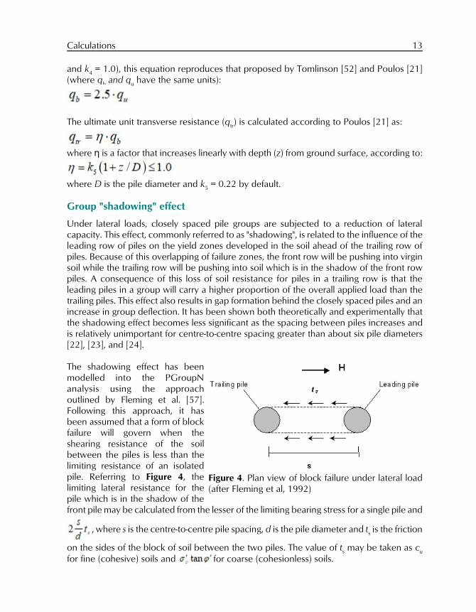
Figure 4. Plan view of block failure under lateral load(after Fleming et al, 1992)
and k4 = 1.0), this equation reproduces that proposed by Tomlinson [52] and Poulos [21](where qb and qu have the same units):
The ultimate unit transverse resistance (qtr) is calculated according to Poulos [21] as:
where 0 is a factor that increases linearly with depth (z) from ground surface, according to:
where D is the pile diameter and k5 = 0.22 by default.
Group "shadowing" effect
Under lateral loads, closely spaced pile groups are subjected to a reduction of lateralcapacity. This effect, commonly referred to as "shadowing", is related to the influence of theleading row of piles on the yield zones developed in the soil ahead of the trailing row ofpiles. Because of this overlapping of failure zones, the front row will be pushing into virginsoil while the trailing row will be pushing into soil which is in the shadow of the front rowpiles. A consequence of this loss of soil resistance for piles in a trailing row is that theleading piles in a group will carry a higher proportion of the overall applied load than thetrailing piles. This effect also results in gap formation behind the closely spaced piles and anincrease in group deflection. It has been shown both theoretically and experimentally thatthe shadowing effect becomes less significant as the spacing between piles increases andis relatively unimportant for centre-to-centre spacing greater than about six pile diameters[22], [23], and [24].
The shadowing effect has beenmodelled into the PGroupNanalysis using the approachoutlined by Fleming et al. [57].Following this approach, it hasbeen assumed that a form of blockfailure will govern when theshearing resistance of the soilbetween the piles is less than thelimiting resistance of an isolatedpile. Referring to Figure 4, thelimiting lateral resistance for thepile which is in the shadow of thefront pile may be calculated from the lesser of the limiting bearing stress for a single pile and
, where s is the centre-to-centre pile spacing, d is the pile diameter and ts is the friction
on the sides of the block of soil between the two piles. The value of ts may be taken as cu
for fine (cohesive) soils and for coarse (cohesionless) soils.
14 Geocentrix Repute 2.5 Reference Manual
The outlined approach provides a simple yet rational means of estimating the shadowingeffect in closely spaced groups, as compared to the purely empirical "p-multiplier" conceptwhich is employed in load-transfer analyses (e.g. in GROUP [25]).
Extension to non-linear soil behaviour
Non-linear soil behaviour has been incorporated by assuming that the soil Young's modulusvaries with the stress level at the pile-soil interface. A simple and popular assumption is toadopt a hyperbolic relationship between soil stress and strain, in which case the tangentYoung's modulus of the soil Etan is given by (see [12], [26], [27]):
where Ei is the initial tangent soil modulus, Rf is the hyperbolic curve-fitting constant, t is thepile-soil stress and ts is the ultimate unit pile-soil stress obtained from equations for thelimiting pile-soil stress. Thus, the boundary element equations described above for the linearresponse are solved incrementally using the modified values of soil Young's modulus ofgiven above and enforcing the conditions of yield, equilibrium and compatibility at thepile-soil interface. For the pile-soil interface elements that have yielded, no more stressincrease is permitted and therefore any increase in load is redistributed between theremaining elastic elements until all elements have failed. It is noted that yielding of anelement introduces a discontinuity in the material property and, therefore, the use ofMindlin's solution to determine the remaining elastic coefficients is only approximate.However, previous work indicates that the errors engendered by this approach are slight(e.g. Basile [2], Poulos [12]).
The hyperbolic curve fitting constant Rf defines the degree of curvature of the stress-strainresponse and can range between 0 (an elastic-perfectly plastic response) and 0.99 (Rf = 1is representative of an asymptotic hyperbolic response in which the limiting pile-soil stressis never reached). Different values of Rf should be used for the axial response of the shaftand the base, for the shaft lateral response, and for the shaft torsional response.
For the axial response of the shaft, values of Rf in the range 0-0.75 are generally used, whilethe base axial response is highly non-linear and therefore values of Rf in the range 0.90-0.99are appropriate (e.g. [12], [28]). For the lateral and torsional response of the shaft, values ofRf in the range 0.50-0.99 generally give a reasonable fit with the observed behaviour.
The best way to determine the values of Rf is by back-fitting the PGroupN load-deformationcurve with the measured data from a full-scale pile loading test. In the absence of any testdata, the values of Rf can be estimated based on experience and, as a preliminaryassessment, the following values may be adopted: Rf = 0.5 (shaft), Rf = 0.99 (base), Rf = 0.9(lateral), and Rf = 0.99 (torsional).
Finally, it should be noted that, in assessing the lateral response of a pile at high load levels,the assumption of a linear elastic model for the pile material becomes less valid and maylead to an underestimation of pile deflections.
Calculations 15
Fleming’s analysis
Fleming’s analysis predicts the load vs settlement behaviour of a single pile. The analysis is based on the method described in Fleming’s paper A new method for single pile settlementprediction and analysis [29].
The total load applied to the pile is given by:
where:Db = base diameterDs = shaft diameterEb = base stiffness (modulus of soil beneath the pile base)P = axial force applied to the pileMs = shaft flexibility factor (0.004 in soft to firm or relatively loose soils; -0.0005 in verystiff soils or soft rock; 0.001-0.002 in stiff overconsolidated clays)s = total pile head settlement, assuming the pile is purely rigidUb = ultimate base loadUs = ultimate shaft load
The above equation can be solved to give the total pile head settlement for any appliedforce:
The elastic shortening of the pile shaft under load can be estimated from:
where:
16 Geocentrix Repute 2.5 Reference Manual
Ec = Young’s modulus of elasticity of the pile material in compressionKE = factor for calculating effective column length (usually -0.45 in stiff overconsolidatedclays)LF = length of pile involved in frictional load transferL0 = length of pile which is friction-free or carries low frictionse = elastic shortening of pile
Values of the parameters are normally found by a curve-fitting exercise. See Fleming’s paper[loc. cit.] for examples. This method is also implemented in the computer program CEMSET,described in that paper.
Longitudinal ULS
Longitudinal ULS checks the ultimate limit state of a single pile under vertical loading.
The design effect of actions Fd is given by:
where:(G = partial factor on permanent actions ($ 1.0)FG,k = characteristic permanent actionR = combination factor (# 1.0)(Q = partial factor on variable actions ($ 1.0)FQ,k = characteristic variable action
The design resistance Rd is given by:
where:fs = skin friction against the pile shaftAs = circumferential area of pile shaft (per unit length)z = depth below ground surfaceL = length of pile shaftqb = unit end-bearing resistance of pile baseAb = area of pile base(s = partial factor on shaft resistance(b = partial factor on base resistance(Rd = model factor on pile resistance
In undrained horizons
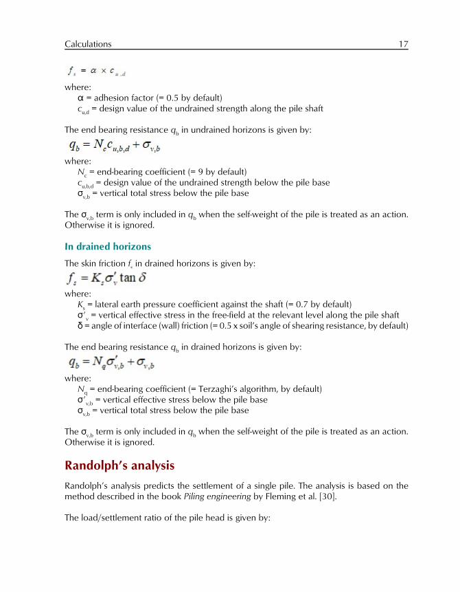
The skin friction fs in undrained horizons is given by:
Calculations 17
where:" = adhesion factor (= 0.5 by default)cu,d = design value of the undrained strength along the pile shaft
The end bearing resistance qb in undrained horizons is given by:
where:Nc = end-bearing coefficient (= 9 by default)cu,b,d = design value of the undrained strength below the pile baseFv,b = vertical total stress below the pile base
The Fv,b term is only included in qb when the self-weight of the pile is treated as an action.Otherwise it is ignored.
In drained horizons
The skin friction fs in drained horizons is given by:
where:Ks = lateral earth pressure coefficient against the shaft (= 0.7 by default)FNv = vertical effective stress in the free-field at the relevant level along the pile shaft* = angle of interface (wall) friction (= 0.5 x soil’s angle of shearing resistance, by default)
The end bearing resistance qb in drained horizons is given by:
where:Nq = end-bearing coefficient (= Terzaghi’s algorithm, by default)FNv,b = vertical effective stress below the pile baseFv,b = vertical total stress below the pile base
The Fv,b term is only included in qb when the self-weight of the pile is treated as an action.Otherwise it is ignored.
Randolph’s analysis
Randolph’s analysis predicts the settlement of a single pile. The analysis is based on themethod described in the book Piling engineering by Fleming et al. [30].
The load/settlement ratio of the pile head is given by:
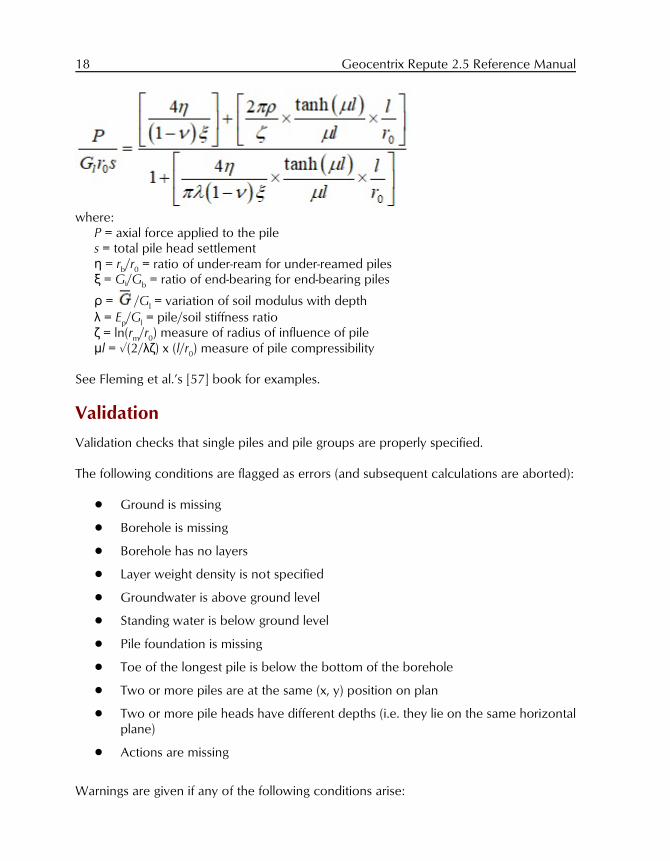
18 Geocentrix Repute 2.5 Reference Manual
where:P = axial force applied to the piles = total pile head settlement0 = rb/r0 = ratio of under-ream for under-reamed piles> = Gl/Gb = ratio of end-bearing for end-bearing piles
D = /Gl = variation of soil modulus with depth8 = Ep/Gl = pile/soil stiffness ratio. = ln(rm/r0) measure of radius of influence of pile:l = %(2/8.) x (l/r0) measure of pile compressibility
See Fleming et al.’s [57] book for examples.
Validation
Validation checks that single piles and pile groups are properly specified.
The following conditions are flagged as errors (and subsequent calculations are aborted):
! Ground is missing
! Borehole is missing
! Borehole has no layers
! Layer weight density is not specified
! Groundwater is above ground level
! Standing water is below ground level
! Pile foundation is missing
! Toe of the longest pile is below the bottom of the borehole
! Two or more piles are at the same (x, y) position on plan
! Two or more pile heads have different depths (i.e. they lie on the same horizontalplane)
! Actions are missing
Warnings are given if any of the following conditions arise:
Calculations 19
! Water table is missing
! Two or more piles are raked towards each other
! Design standard is missing
In addition, when a boundary element analysis is performed, the following conditions areflagged as errors (and the subsequent analysis is aborted):
! Number of piles exceeds 350
! Number of layers exceeds 50
! Number of pile elements is less than 3 or greater than 50
! Number of load increments is greater than 500
! Torque is applied to the pile group and one or more piles have an asymmetricalrake: if the pile is double-raked (in both the X and Y directions), then it must besymmetrically raked, i.e. the absolute values of the angles of rake in the X and Ydirections must be the same (only when torsion loading is present)
! Piles are too close together (i.e. the smallest spacing to diameter ratio is less than2.5)
! Piles are too stubby (i.e. the smallest slenderness ratio is less than 5)
! Layer stiffness is not specified (large-strain stiffness is checked for linear-elastic andlinear-elastic/perfectly-plastic analyses; small-strain stiffness for a non-linear analysis)
20 Geocentrix Repute 2.5 Reference Manual
Chapter 3Design standards
Repute supports the following design standards:
! British Standard BS 8004: 1986 [31], now superseded by BS 8004: 2015
! Draft Eurocode 7 ENV 1997-1: 1994 [32], now superseded by Eurocode 7
! Eurocode 7 EN 1997-1: 2004 [33], with no National Annex
! British Standard BS EN 1997-1:2004+A1:2013 [34], Eurocode 7 with the UKNational Annex
! Irish Standard IS EN 1997-1: 2007 [35], Eurocode 7 with the Irish National Annex
! NTC08 (Italian National Building Code) 2008 [36]
! Singapore Standard SS EN 1997-1: 2010 [37], Eurocode 7 with the SingaporeNational Annex
! British Standard BS 8004: 2015 [38]
! Custom Working Stress, user-defined (with default values from BS 8004:1986)
! Custom Eurocode 7, user-defined (with default values from Eurocode 7)
Partial (safety) factors
The following symbols are used in this chapter to represent partial (and other safety) factorsthat are employed in pile design.
(G partial factor on (unfavourable) permanent action(Q partial factor on (unfavourable) variable action(A partial factor on (unfavourable) accidental action(G,fav partial factor on favourable permanent action(b partial factor on base resistance of pile(s partial factor on shaft resistance of pile(t partial factor on total (i.e. shaft + base) resistance of pile(st partial factor on shaft resistance of pile in tension(Rd model factor on pile resistance(n partial factor on coefficient of shearing resistance of soil(c partial factor on effective cohesion of soil(cu partial factor on undrained strength of soil(qu partial factor on unconfined compressive strength of rock
The values of these factors are given in the following table.
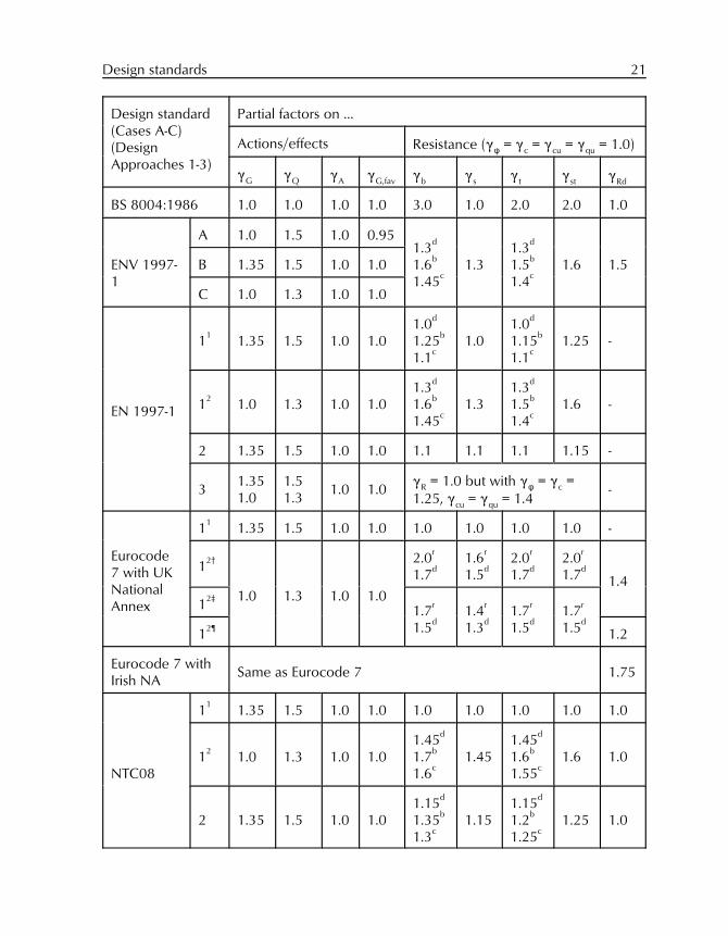
Design standards 21
Design standard(Cases A-C)(DesignApproaches 1-3)
Partial factors on ...
Actions/effects Resistance ((n = (c = (cu = (qu = 1.0)
(G (Q (A (G,fav (b (s (t (st (Rd
BS 8004:1986 1.0 1.0 1.0 1.0 3.0 1.0 2.0 2.0 1.0
ENV 1997-1
A 1.0 1.5 1.0 0.951.3
d
1.6b
1.45c
1.31.3
d
1.5b
1.4c
1.6 1.5B 1.35 1.5 1.0 1.0
C 1.0 1.3 1.0 1.0
EN 1997-1
11
1.35 1.5 1.0 1.01.0
d
1.25b
1.1c
1.01.0
d
1.15b
1.1c
1.25 -
12
1.0 1.3 1.0 1.01.3
d
1.6b
1.45c
1.31.3
d
1.5b
1.4c
1.6 -
2 1.35 1.5 1.0 1.0 1.1 1.1 1.1 1.15 -
31.351.0
1.51.3
1.0 1.0(R = 1.0 but with (n = (c =1.25, (cu = (qu = 1.4
-
Eurocode7 with UKNationalAnnex
11
1.35 1.5 1.0 1.0 1.0 1.0 1.0 1.0 -
12†
1.0 1.3 1.0 1.0
2.0r
1.7d
1.6r
1.5d
2.0r
1.7d
2.0r
1.7d
1.4
12‡
1.7r
1.5d
1.4r
1.3d
1.7r
1.5d
1.7r
1.5d
12¶
1.2
Eurocode 7 withIrish NA
Same as Eurocode 7 1.75
NTC08
11
1.35 1.5 1.0 1.0 1.0 1.0 1.0 1.0 1.0
12
1.0 1.3 1.0 1.01.45
d
1.7b
1.6c
1.451.45
d
1.6b
1.55c
1.6 1.0
2 1.35 1.5 1.0 1.01.15
d
1.35b
1.3c
1.151.15
d
1.2b
1.25c
1.25 1.0
22 Geocentrix Repute 2.5 Reference Manual
Design standard(Cases A-C)(DesignApproaches 1-3)
Partial factors on ...
Actions/effects Resistance ((n = (c = (cu = (qu = 1.0)
(G (Q (A (G,fav (b (s (t (st (Rd
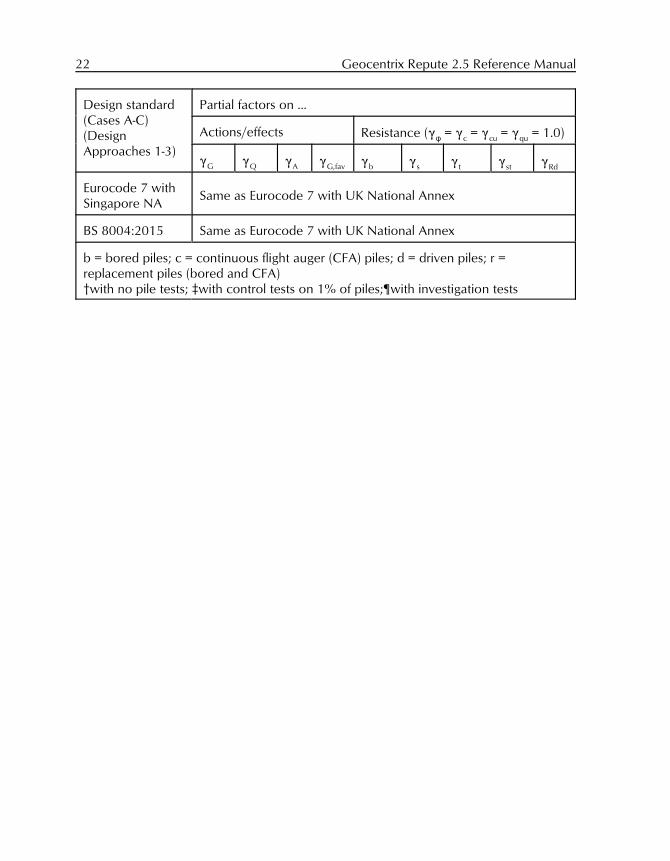
Eurocode 7 withSingapore NA
Same as Eurocode 7 with UK National Annex
BS 8004:2015 Same as Eurocode 7 with UK National Annex
b = bored piles; c = continuous flight auger (CFA) piles; d = driven piles; r =replacement piles (bored and CFA)†with no pile tests; ‡with control tests on 1% of piles;¶with investigation tests
Actions 23
Figure 5. Sign convention used in Repute 2 for (top-left) forces, (top-right) moments, (bottom-left) displacements, (bottom-right) rotations
Chapter 4Actions
Repute® implements the following actions:
! Combinations of actions
! Forces
! Moments
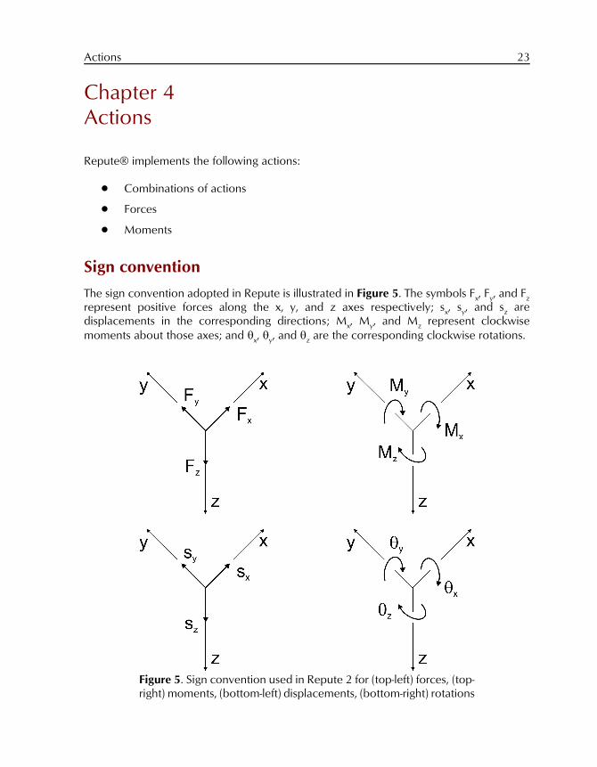
Sign convention
The sign convention adopted in Repute is illustrated in Figure 5. The symbols Fx, Fy, and Fz
represent positive forces along the x, y, and z axes respectively; sx, sy, and sz aredisplacements in the corresponding directions; Mx, My, and Mz represent clockwisemoments about those axes; and qx, qy, and qz are the corresponding clockwise rotations.
24 Geocentrix Repute 2.5 Reference Manual
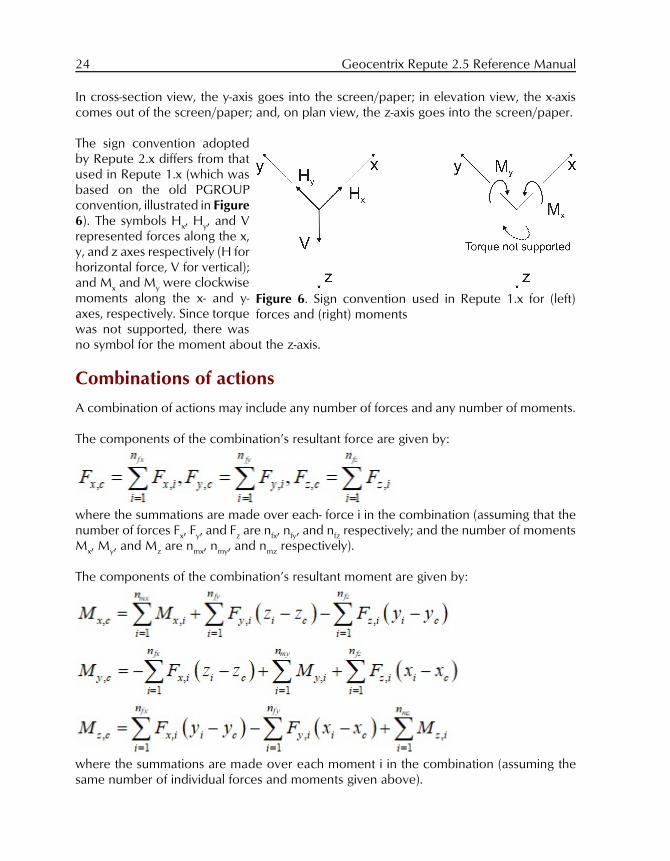
Figure 6. Sign convention used in Repute 1.x for (left)forces and (right) moments
In cross-section view, the y-axis goes into the screen/paper; in elevation view, the x-axiscomes out of the screen/paper; and, on plan view, the z-axis goes into the screen/paper.
The sign convention adoptedby Repute 2.x differs from thatused in Repute 1.x (which wasbased on the old PGROUPconvention, illustrated in Figure6). The symbols Hx, Hy, and Vrepresented forces along the x,y, and z axes respectively (H forhorizontal force, V for vertical); and Mx and My were clockwisemoments along the x- and y-axes, respectively. Since torquewas not supported, there wasno symbol for the moment about the z-axis.
Combinations of actions
A combination of actions may include any number of forces and any number of moments.
The components of the combination’s resultant force are given by:
where the summations are made over each- force i in the combination (assuming that thenumber of forces Fx, Fy, and Fz are nfx, nfy, and nfz respectively; and the number of momentsMx, My, and Mz are nmx, nmy, and nmz respectively).
The components of the combination’s resultant moment are given by:
where the summations are made over each moment i in the combination (assuming thesame number of individual forces and moments given above).
Actions 25
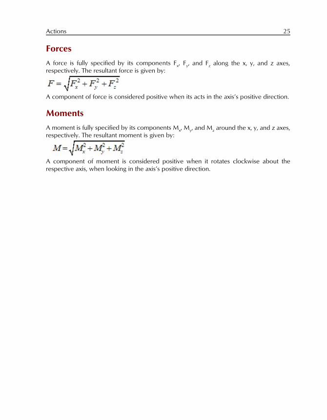
Forces
A force is fully specified by its components Fx, Fy, and Fz along the x, y, and z axes,respectively. The resultant force is given by:
A component of force is considered positive when its acts in the axis’s positive direction.
Moments
A moment is fully specified by its components Mx, My, and Mz around the x, y, and z axes,respectively. The resultant moment is given by:
A component of moment is considered positive when it rotates clockwise about therespective axis, when looking in the axis’s positive direction.
26 Geocentrix Repute 2.5 Reference Manual
Chapter 5Material and section properties
Repute® allows you to specify properties for the following materials:
! Soils
! Concretes
! Steels
Repute also allows you to specify properties for the following sections:
! Bearing piles
! Circular section
! Custom section
! Rectangular section
Soils
Repute implements the following soils:
! Gravel, Sand, Coarse Silt, Granular Fill, and Custom Granular Soil
! Silt, Clay, Cohesive Fill, Organic Soil, River Soil, and Custom Cohesive Soil
! Chalk, Rock
These soils are further described according to the Re/x Soil Classification System, which isbased on the terms defined in EN ISOs 14688 [39] and 14689 [40].
The following table lists the soils that are included in the Re/x Soil Classification System andgive the corresponding group symbols from each of the established systems listed above(where they are available).
Soil Symbol Class Possible states
Gravel GrCGrMGrFGrsiGrclGr
GRAVEL*Coarse GRAVELMedium GRAVELFine GRAVELsilty GRAVELclayey GRAVEL*
Unspecified (-)Very loose (V. loose)¶LooseMedium dense (Med. dense)DenseVery dense (V. dense)
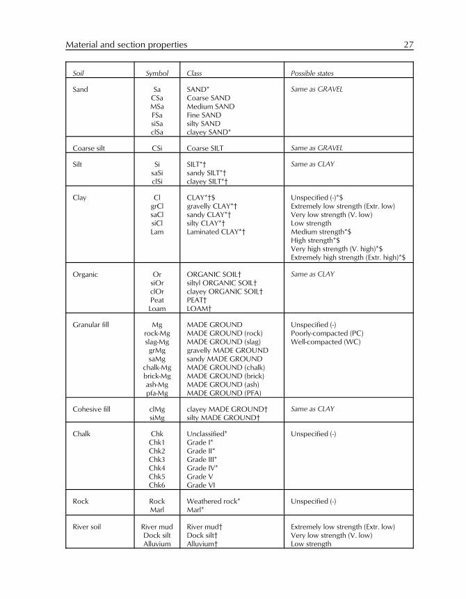
Material and section properties 27
Soil Symbol Class Possible states
Sand SaCSaMSaFSasiSaclSa
SAND*Coarse SANDMedium SANDFine SANDsilty SANDclayey SAND*
Same as GRAVEL
Coarse silt CSi Coarse SILT Same as GRAVEL
Silt SisaSiclSi
SILT*†sandy SILT*†clayey SILT*†
Same as CLAY
Clay ClgrClsaClsiClLam
CLAY*†$gravelly CLAY*†sandy CLAY*†silty CLAY*†Laminated CLAY*†
Unspecified (-)*$Extremely low strength (Extr. low)Very low strength (V. low)Low strengthMedium strength*$High strength*$Very high strength (V. high)*$Extremely high strength (Extr. high)*$
Organic OrsiOrclOrPeatLoam
ORGANIC SOIL†siltyl ORGANIC SOIL†clayey ORGANIC SOIL†PEAT†LOAM†
Same as CLAY
Granular fill Mgrock-Mgslag-MggrMgsaMg
chalk-Mgbrick-Mgash-Mgpfa-Mg
MADE GROUNDMADE GROUND (rock)MADE GROUND (slag)gravelly MADE GROUNDsandy MADE GROUNDMADE GROUND (chalk)MADE GROUND (brick)MADE GROUND (ash)MADE GROUND (PFA)
Unspecified (-)Poorly-compacted (PC)Well-compacted (WC)
Cohesive fill clMgsiMg
clayey MADE GROUND†silty MADE GROUND†
Same as CLAY
Chalk ChkChk1Chk2Chk3Chk4Chk5Chk6
Unclassified*Grade I*Grade II*Grade III*Grade IV*Grade VGrade VI
Unspecified (-)
Rock RockMarl
Weathered rock*Marl*
Unspecified (-)
River soil River mudDock siltAlluvium
River mud†Dock silt†Alluvium†
Extremely low strength (Extr. low)Very low strength (V. low)Low strength
28 Geocentrix Repute 2.5 Reference Manual
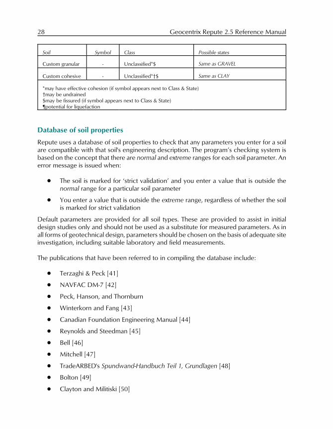
Soil Symbol Class Possible states
Custom granular - Unclassified*$ Same as GRAVEL
Custom cohesive - Unclassified*†$ Same as CLAY
*may have effective cohesion (if symbol appears next to Class & State)†may be undrained$may be fissured (if symbol appears next to Class & State)¶potential for liquefaction
Database of soil properties
Repute uses a database of soil properties to check that any parameters you enter for a soilare compatible with that soil's engineering description. The program’s checking system isbased on the concept that there are normal and extreme ranges for each soil parameter. Anerror message is issued when:
! The soil is marked for ‘strict validation’ and you enter a value that is outside thenormal range for a particular soil parameter
! You enter a value that is outside the extreme range, regardless of whether the soilis marked for strict validation
Default parameters are provided for all soil types. These are provided to assist in initialdesign studies only and should not be used as a substitute for measured parameters. As inall forms of geotechnical design, parameters should be chosen on the basis of adequate siteinvestigation, including suitable laboratory and field measurements.
The publications that have been referred to in compiling the database include:
! Terzaghi & Peck [41]
! NAVFAC DM-7 [42]
! Peck, Hanson, and Thornburn
! Winterkorn and Fang [43]
! Canadian Foundation Engineering Manual [44]
! Reynolds and Steedman [45]
! Bell [46]
! Mitchell [47]
! TradeARBED's Spundwand-Handbuch Teil 1, Grundlagen [48]
! Bolton [49]
! Clayton and Militiski [50]
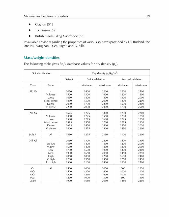
Material and section properties 29
! Clayton [51]
! Tomlinson [52]
! British Steel's Piling Handbook [53]
Invaluable advice regarding the properties of various soils was provided by J.B. Burland, thelate P.R. Vaughan, D.W. Hight, and G. Sills.
Mass/weight densities
The following table gives Re/x database values for dry density (Dd).
Soil classification Dry density Dd (kg/m3)
Default Strict validation Relaxed validation
Class State Minimum Maximum Minimum Maximum
(All) Gr -V. looseLoose
Med. denseDense
V. dense
205015001650185020502250
140013001400150017002000
220016001800200022002400
120012001300140015001700
250018002000220024002500
(All) Sa -V. looseLoose
Med. denseDense
V. dense
167514501500157516751800
127512251275135014501575
180015501600170018001900
120012001225127513501450
220017501850195020502200
(All) Si All 1850 1275 2150 1100 2200
(All) Cl -Ext. lowV. lowLowMedHigh
V. highExt. high
20501650165017501900205022002300
15001400140015001650180019502100
22001800180019002050220023502400
12001200120013001450160017501900
25002000200021002250240024502500
OrsiOrclOrPeatLoam
All 15001500150012001900
10001250125010001650
20501600160013002050
800100010008001450
22501750175014002250
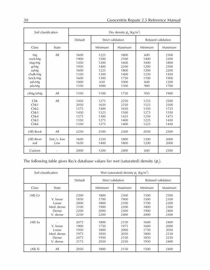
30 Geocentrix Repute 2.5 Reference Manual
Soil classification Dry density Dd (kg/m3)
Default Strict validation Relaxed validation
Class State Minimum Maximum Minimum Maximum
Mgrock-Mgslag-MggrMgsaMg
chalk-Mgbrick-Mgash-Mgpfa-Mg
All 160019001450195016001350160010001350
12251500120014001225130013006501000
180021001600220018001400175010001500
600140010001200120012501100600900
250022001800250022001450190012001700
clMg/siMg All 1550 1100 1750 950 1900
ChkChk1Chk2Chk3Chk4Chk5Chk6
All 1450205015751450137513501350
1275165014001325130012751275
2250225016501500142514001400
1255152513501275125012251225
2500250017251550147514501450
(All) Rock All 2250 2100 2300 2050 2500
(All) Riversoil
Extr./v. lowLow
16001650
12501400
18001800
12001200
20002000
Custom - 2000 1200 2400 600 2500
The following table gives Re/x database values for wet (saturated) density (Ds).
Soil classification Wet (saturated) density Ds (kg/m3)
Default Strict validation Relaxed validation
Class State Minimum Maximum Minimum Maximum
(All) Gr -V. looseLoose
Med. denseDense
V. dense
220018502000210022002250
180017001800190020002200
230019002100220023002400
150015001700180019002000
250021002200230024002500
(All) Sa -V. looseLoose
Med. denseDense
V. dense
207519001950197520752175
180017501800185019502050
215019752000205021502250
160016001750180018501950
240020002050215022502400
(All) Si All 2050 1800 2150 1500 2400
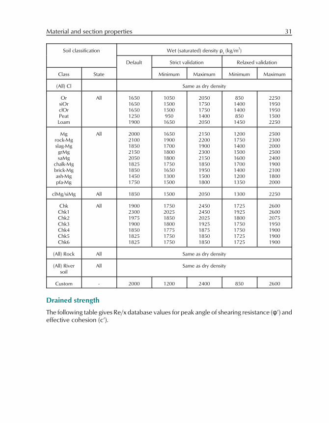
Material and section properties 31
Soil classification Wet (saturated) density Ds (kg/m3)
Default Strict validation Relaxed validation
Class State Minimum Maximum Minimum Maximum
(All) Cl Same as dry density
OrsiOrclOrPeatLoam
All 16501650165012501900
1050150015009501650
20501750175014002050
850140014008501450
22501950195015002250
Mgrock-Mgslag-MggrMgsaMg
chalk-Mgbrick-Mgash-Mgpfa-Mg
All 200021001850215020501825185014501750
165019001700180018001750165013001500
215022001900230021501850195015001800
120017501400150016001700140012001350
250023002000250024001900210018002000
clMg/siMg All 1850 1500 2050 1300 2250
ChkChk1Chk2Chk3Chk4Chk5Chk6
All 1900230019751900185018251825
1750202518501800177517501750
2450245020251925187518501850
1725192518001750175017251725
2600260020751950190019001900
(All) Rock All Same as dry density
(All) Riversoil
All Same as dry density
Custom - 2000 1200 2400 850 2600
Drained strength
The following table gives Re/x database values for peak angle of shearing resistance (n’) andeffective cohesion (c’).
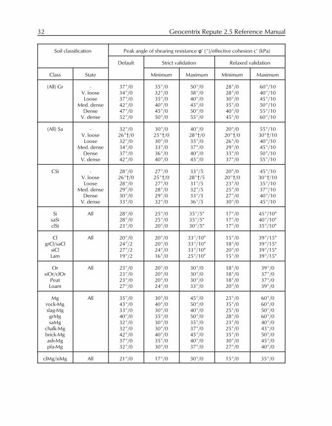
32 Geocentrix Repute 2.5 Reference Manual
Soil classification Peak angle of shearing resistance n’ (E)/effective cohesion c’ (kPa)
Default Strict validation Relaxed validation
Class State Minimum Maximum Minimum Maximum
(All) Gr -V. looseLoose
Med. denseDense
V. dense
37E/034E/037E/042E/047E/052E/0
35E/032E/035E/040E/045E/050E/0
50E/038E/040E/045E/050E/055E/0
28E/028E/030E/035E/040E/045E/0
60E/1040E/1045E/1050E/1055E/1060E/10
(All) Sa -V. looseLoose
Med. denseDense
V. dense
32E/026E†/032E/034E/037E/042E/0
30E/025E†/030E/033E/036E/040E/0
40E/028E†/035E/037E/040E/045E/0
20E/020E†/026E/029E/033E/037E/0
55E/1030E†/1040E/1045E/1050E/1055E/10
CSi -V. looseLoose
Med. denseDense
V. dense
28E/026E†/028E/029E/030E/033E/0
27E/025E†/027E/028E/029E/032E/0
33E/528E†/531E/532E/533E/536E/5
20E/020E†/023E/025E/027E/030E/0
45E/1030E†/1035E/1037E/1040E/1045E/10
SisaSiclSi
All 28E/028E/023E/0
25E/025E/020E/0
35E/5*35E/5*30E/5*
17E/017E/017E/0
45E/10*40E/10*35E/10*
ClgrCl/saCl
siClLam
All 20E/024E/227E/219E/2
20E/020E/024E/016E/0
33E/10*33E/10*33E/10*25E/10*
15E/018E/020E/015E/0
39E/15*39E/15*39E/15*39E/15*
OrsiOr/clOr
PeatLoam
All 23E/023E/023E/027E/0
20E/020E/020E/024E/0
30E/030E/030E/033E/0
18E/018E/018E/020E/0
39E/037E/037E/039E/0
Mgrock-Mgslag-MggrMgsaMg
chalk-Mgbrick-Mgash-Mgpfa-Mg
All 35E/043E/033E/040E/032E/032E/042E/037E/032E/0
30E/040E/030E/035E/030E/030E/040E/035E/030E/0
45E/050E/040E/050E/035E/037E/045E/040E/037E/0
23E/035E/025E/028E/023E/025E/035E/030E/027E/0
60E/060E/050E/060E/040E/043E/050E/045E/040E/0
clMg/siMg All 21E/0 17E/0 30E/0 15E/0 35E/0
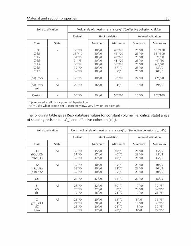
Material and section properties 33
Soil classification Peak angle of shearing resistance n’ (E)/effective cohesion c’ (kPa)
Default Strict validation Relaxed validation
Class State Minimum Maximum Minimum Maximum
ChkChk1Chk2Chk3Chk4Chk5Chk6
- 35E/035E/1034E/534E/533E/232E/032E/0
30E/030E/030E/030E/030E/030E/030E/0
45E/2045E/2043E/2041E/2039E/1037E/035E/0
25E/025E/025E/025E/025E/025E/025E/0
55E/10055E/10052E/5049E/5046E/2043E/040E/0
(All) Rock - 33E/5 30E/0 38E/10 27E/0 42E/20
(All) Riversoil
All 22E/0 16E/0 33E/0 15E/0 39E/0
Custom - 30E/0 20E/0 50E/10 10E/0 60E/100
†n’ reduced to allow for potential liquefaction*c’ = 0kPa when state is set to extremely low, very low, or low strength
The following table gives Re/x database values for constant volume (i.e. critical state) angleof shearing resistance (n’cv) and effective cohesion (c’cv).
Soil classification Const. vol. angle of shearing resistance n’cv (E)/effective cohesion c’cv (kPa)
Default Strict validation Relaxed validation
Class State Minimum Maximum Minimum Maximum
- GrsiGr/clGr(other) Gr
All 37E/037E/037E/0
35E/037E/037E/0
40E/040E/040E/0
28E/028E/028E/0
45E/545E/545E/0
- SasiSa/clSa(other) Sa
All 32E/032E/032E/0
30E/030E/030E/0
35E/035E/035E/0
23E/023E/023E/0
40E/540E/540E/0
CSi - 28E/0 27E/0 31E/0 20E/0 35E/5
SisaSiclSi
All 25E/025E/019E/0
22E/022E/018E/0
30E/030E/022E/0
17E/020E/017E/0
32E/5*32E/5*25E/5*
ClgrCl/saCl
siClLam
All 23E/024E/023E/016E/0
20E/020E/020E/012E/0
33E/033E/028E/020E/0
8E/018E/018E/08E/0
39E/5*39E/5*30E/5*22E/5*
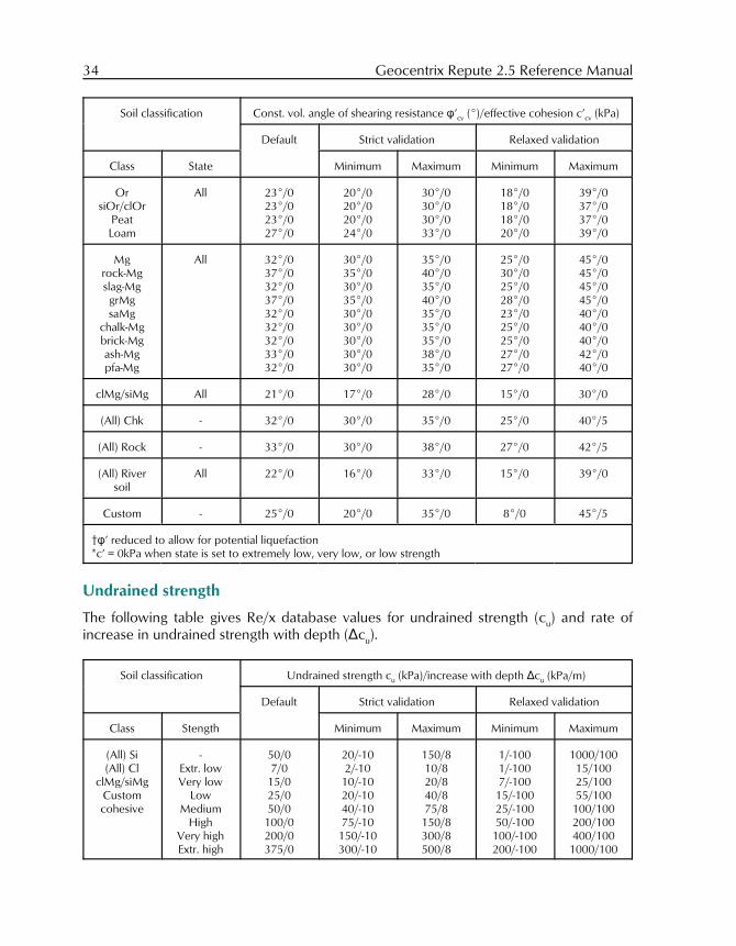
34 Geocentrix Repute 2.5 Reference Manual
Soil classification Const. vol. angle of shearing resistance n’cv (E)/effective cohesion c’cv (kPa)
Default Strict validation Relaxed validation
Class State Minimum Maximum Minimum Maximum
OrsiOr/clOr
PeatLoam
All 23E/023E/023E/027E/0
20E/020E/020E/024E/0
30E/030E/030E/033E/0
18E/018E/018E/020E/0
39E/037E/037E/039E/0
Mgrock-Mgslag-MggrMgsaMg
chalk-Mgbrick-Mgash-Mgpfa-Mg
All 32E/037E/032E/037E/032E/032E/032E/033E/032E/0
30E/035E/030E/035E/030E/030E/030E/030E/030E/0
35E/040E/035E/040E/035E/035E/035E/038E/035E/0
25E/030E/025E/028E/023E/025E/025E/027E/027E/0
45E/045E/045E/045E/040E/040E/040E/042E/040E/0
clMg/siMg All 21E/0 17E/0 28E/0 15E/0 30E/0
(All) Chk - 32E/0 30E/0 35E/0 25E/0 40E/5
(All) Rock - 33E/0 30E/0 38E/0 27E/0 42E/5
(All) Riversoil
All 22E/0 16E/0 33E/0 15E/0 39E/0
Custom - 25E/0 20E/0 35E/0 8E/0 45E/5
†n’ reduced to allow for potential liquefaction*c’ = 0kPa when state is set to extremely low, very low, or low strength
Undrained strength
The following table gives Re/x database values for undrained strength (cu) and rate ofincrease in undrained strength with depth ()cu).
Soil classification Undrained strength cu (kPa)/increase with depth )cu (kPa/m)
Default Strict validation Relaxed validation
Class Stength Minimum Maximum Minimum Maximum
(All) Si(All) Cl
clMg/siMgCustomcohesive
-Extr. lowVery low
LowMedium
HighVery highExtr. high
50/07/015/025/050/0100/0200/0375/0
20/-102/-1010/-1020/-1040/-1075/-10150/-10300/-10
150/810/820/840/875/8150/8300/8500/8
1/-1001/-1007/-10015/-10025/-10050/-100100/-100200/-100
1000/10015/10025/10055/100100/100200/100400/1001000/100
Material and section properties 35
Soil classification Undrained strength cu (kPa)/increase with depth )cu (kPa/m)
Default Strict validation Relaxed validation
Class Stength Minimum Maximum Minimum Maximum
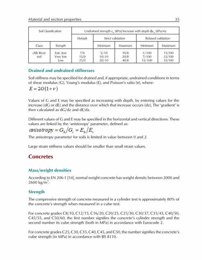
(All) Riversoil
Extr. lowVery low
Low
7/015/025/0
5/-1010/-1020/-10
10/820/840/8
1/-1007/-10015/-100
15/10025/10055/100
Drained and undrained stiffnesses
Soil stiffness may be specified for drained and, if appropriate, undrained conditions in termsof shear modulus (G), Young’s modulus (E), and Poisson’s ratio (<), where:
Values of G and E may be specified as increasing with depth, by entering values for theincrease (dG or dE) and the distance over which that increase occurs (dz), The ‘gradient’ isthen calculated as dG/dz and dE/dz.
Different values of G and E may be specified in the horizontal and vertical directions. Thesevalues are linked by the ‘anistoropy’ parameter, defined as:
The anisotropy parameter for soils is limited in value between 0 and 2.
Large strain stiffness values should be smaller than small strain values.
Concretes
Mass/weight densities
According to EN 206-1 [54], normal weight concrete has weight density between 2000 and2600 kg/m
3.
Strength
The compressive strength of concrete measured in a cylinder test is approximately 80% ofthe concrete’s strength when measured in a cube test.
For concrete grades C8/10, C12/15, C16/20, C20/25, C25/30, C30/37, C35/45, C40/50,C45/55, and C50/60, the first number signifies the concrete’s cylinder strength and thesecond number its cube strength (both in MPa) in accordance with Eurocode 2.
For concrete grades C25, C30, C35, C40, C45, and C50, the number signifies the concrete’scube strength (in MPa) in accordance with BS 8110.
36 Geocentrix Repute 2.5 Reference Manual
According to Arya [55], the strength of concrete varies from 12 to 60 MPa.
Stiffness
According to EN 1992-1-1 [56], the Young’s modulus of elasticity for concrete is between27 and 44 GPa. Fleming [57] quotes values between 5 and 40 GPa for foundation concrete.
Different values of Young’s modulus may be specified in the horizontal and verticaldirections. These values are linked by the ‘anistoropy’ parameter, defined as:
The anisotropy parameter for concrete is limited in value between 0 and 1.
Steels
Mass/weight densities
According to EN 1993-1-1 [58] §3.2.6, structural steel has a weight density of 7850 kg/m3.
Strength
For structural steel grades S235, S275, S355, and S450, the number signifies the steel’s yieldstrength.
For Corus’s Advance range of steels (Advance 275 and Advance 355), the number alsosignifies the steel’s yield strength.
Stiffness
According to EN 1993-1-1 [59] §3.2.6, the Young’s modulus of elasticity for structural steelis 210 GPa and its Poisson’s ratio is 0.3.
Bearing piles
The properties of Corus’s UKBP range of bearing piles areprovided in the folder [R]\Sections\Bearing Piles,each in a separate XML file (e.g. UKBP 203x203x45.xml).
The figure (right) shows the key dimensions of an I-section, withnotation taken from EN 1993-1-1:
! Width (b)
! Depth (h)
! Web thickness (tw)
! Flange thickness (tf)
Material and section properties 37
! Depth between fillets (d)
! Root radius (r)
The section’s strong (y-y) and weak (z-z) axes are also shown. The x-x axis runs along thelength of the bearing pile (perpendicular to the plane of the paper).
Circular section
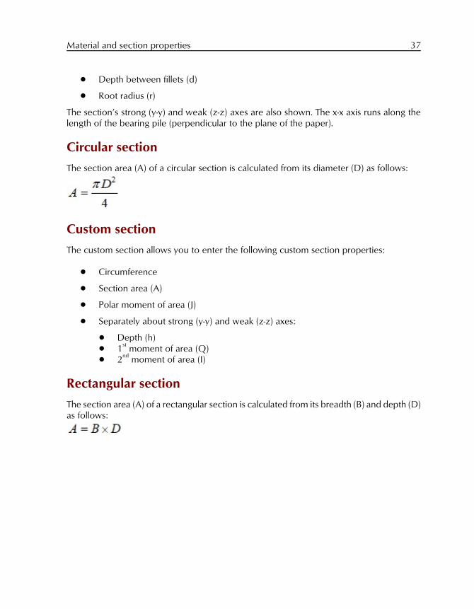
The section area (A) of a circular section is calculated from its diameter (D) as follows:
Custom section
The custom section allows you to enter the following custom section properties:
! Circumference
! Section area (A)
! Polar moment of area (J)
! Separately about strong (y-y) and weak (z-z) axes:
! Depth (h)! 1
st moment of area (Q)
! 2nd
moment of area (I)
Rectangular section
The section area (A) of a rectangular section is calculated from its breadth (B) and depth (D)as follows:
38 Geocentrix Repute 2.5 Reference Manual
Chapter 6Algorithms
Algorithms allow you to change the way calculations are performed. Repute® implementsthe following algorithms:
! Alpha algorithm
! Bearing capacity algorithm
! Bearing pressure limit
! Beta algorithm
! Lateral earth pressure coefficient
! Plugging algorithm
! Shrinkage algorithm
! Skin friction limit
! Wall friction algorithm
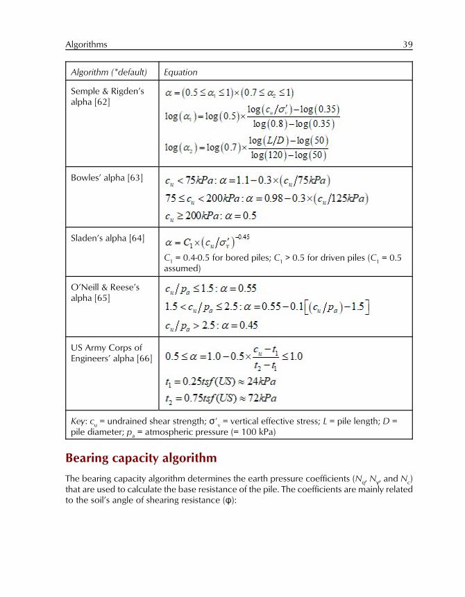
Alpha algorithm
The alpha algorithm determines the skin friction (fs) along the pile shaft in undrainedhorizons, as a proportion of the soil’s undrained strength (cu):
The options for determining " are summarized below.
Algorithm (*default) Equation
Custom alpha " = any value > 0 and # 1
Skempton’s alpha[60]*
" = 0.45
Alpha = 0.5 " = 0.5
Alpha for LondonClay
" = 0.6
Randolph &Murphy’s alpha [61]
Algorithms 39
Algorithm (*default) Equation
Semple & Rigden’salpha [62]
Bowles’ alpha [63]
Sladen’s alpha [64]
C1 = 0.4-0.5 for bored piles; C1 > 0.5 for driven piles (C1 = 0.5assumed)
O’Neill & Reese’salpha [65]
US Army Corps ofEngineers’ alpha [66]
Key: cu = undrained shear strength; FNv = vertical effective stress; L = pile length; D =pile diameter; pa = atmospheric pressure (= 100 kPa)
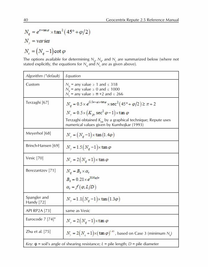
Bearing capacity algorithm
The bearing capacity algorithm determines the earth pressure coefficients (Nq, N(, and Nc)that are used to calculate the base resistance of the pile. The coefficients are mainly relatedto the soil’s angle of shearing resistance (n):
40 Geocentrix Repute 2.5 Reference Manual
The options available for determining Nq, N(, and Nc are summarized below (where notstated explicitly, the equations for Nq and Nc are as given above).
Algorithm (*default) Equation
Custom Nq = any value $ 1 and # 318N( = any value $ 0 and # 1000Nc = any value $ B +2 and # 266
Terzaghi [67]
Terzaghi obtained Kp( by a graphical technique; Repute usesnumerical values given by Kumhojkar (1993)
Meyerhof [68]
Brinch-Hansen [69]
Vesic [70]
Berezantzev [71]
Spangler andHandy [72]
API RP2A [73] same as Vesic
Eurocode 7 [74]*
Zhu et al. [75] , based on Case 3 (minimum N()
Key: n = soil’s angle of shearing resistance; L = pile length; D = pile diameter
Algorithms 41
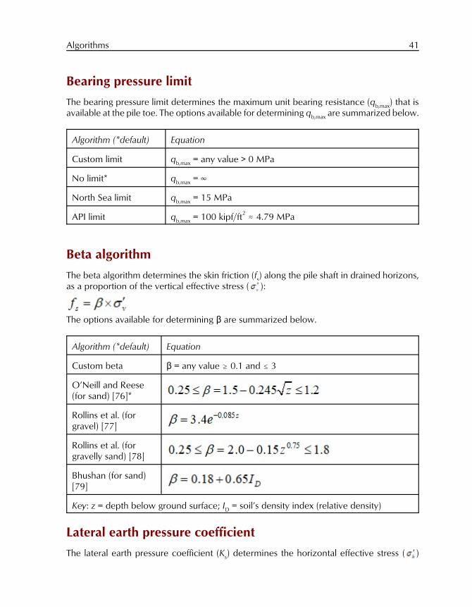
Bearing pressure limit
The bearing pressure limit determines the maximum unit bearing resistance (qb,max) that isavailable at the pile toe. The options available for determining qb,max are summarized below.
Algorithm (*default) Equation
Custom limit qb,max = any value > 0 MPa
No limit* qb,max = 4
North Sea limit qb,max = 15 MPa
API limit qb,max = 100 kipf/ft2 . 4.79 MPa
Beta algorithm
The beta algorithm determines the skin friction (fs) along the pile shaft in drained horizons,as a proportion of the vertical effective stress ( ):
The options available for determining $ are summarized below.
Algorithm (*default) Equation
Custom beta $ = any value $ 0.1 and # 3
O’Neill and Reese(for sand) [76]*
Rollins et al. (forgravel) [77]
Rollins et al. (forgravelly sand) [78]
Bhushan (for sand)[79]
Key: z = depth below ground surface; ID = soil’s density index (relative density)
Lateral earth pressure coefficient
The lateral earth pressure coefficient (Ks) determines the horizontal effective stress ( )
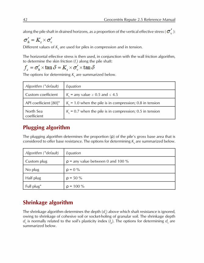
42 Geocentrix Repute 2.5 Reference Manual
along the pile shaft in drained horizons, as a proportion of the vertical effective stress ( ):
Different values of Ks are used for piles in compression and in tension.
The horizontal effective stress is then used, in conjunction with the wall friction algorithm,to determine the skin friction (fs) along the pile shaft:
The options for determining Ks are summarized below.
Algorithm (*default) Equation
Custom coefficient Ks = any value $ 0.5 and # 4.5
API coefficient [80]* Ks = 1.0 when the pile is in compression; 0.8 in tension
North Seacoefficient
Ks = 0.7 when the pile is in compression; 0.5 in tension
Plugging algorithm
The plugging algorithm determines the proportion (D) of the pile’s gross base area that isconsidered to offer base resistance. The options for determining Ks are summarized below.
Algorithm (*default) Equation
Custom plug D = any value between 0 and 100 %
No plug D = 0 %
Half plug D = 50 %
Full plug* D = 100 %
Shrinkage algorithm
The shrinkage algorithm determines the depth (ds) above which shaft resistance is ignored,owing to shrinkage of cohesive soil or socket-holing of granular soil. The shrinkage depthds is normally related to the soil’s plasticity index (Ip). The options for determining ds aresummarized below.

Algorithms 43
Algorithm (*default) Equation
Custom shrinkage ds = any value > 0 m and # 12 m
NHBC (1992) [81]* Ip > 0.4: ds = 1.0 m0.2 < Ip # 0.4: ds = 0.9 mIp # 0.2: ds = 0.75 m
Key: Ip = soil’s plasticity index
Skin friction limit
The skin friction pressure limit determines the maximum unit shaft resistance (qs,max) that isavailable along the pile shaft. The options available for determining qs,max are summarizedbelow.
Algorithm (*default) Equation
Custom limit qs,max = any value > 0 kPa
No limit* qs,max = 4
North Sea limit qs,max = 100 kPa
API limit qs,max = 1700 lbf/ft2 . 81.4 kPa
Wall friction algorithm
The wall friction algorithm determines the skin friction (fs) along the pile shaft, as aproportion of the horizontal effective stress ( ):
The wall friction * is often calculated as a proportion of the soil’s angle of shearingresistance (n).
The horizontal effective stress is obtained from the lateral earth pressure coefficient (Ks) anddepends the vertical effective stress ( ):
The options for determining * are summarized below.
Algorithm (*default) Equation
Custom friction * = any value > 0E and # 35E
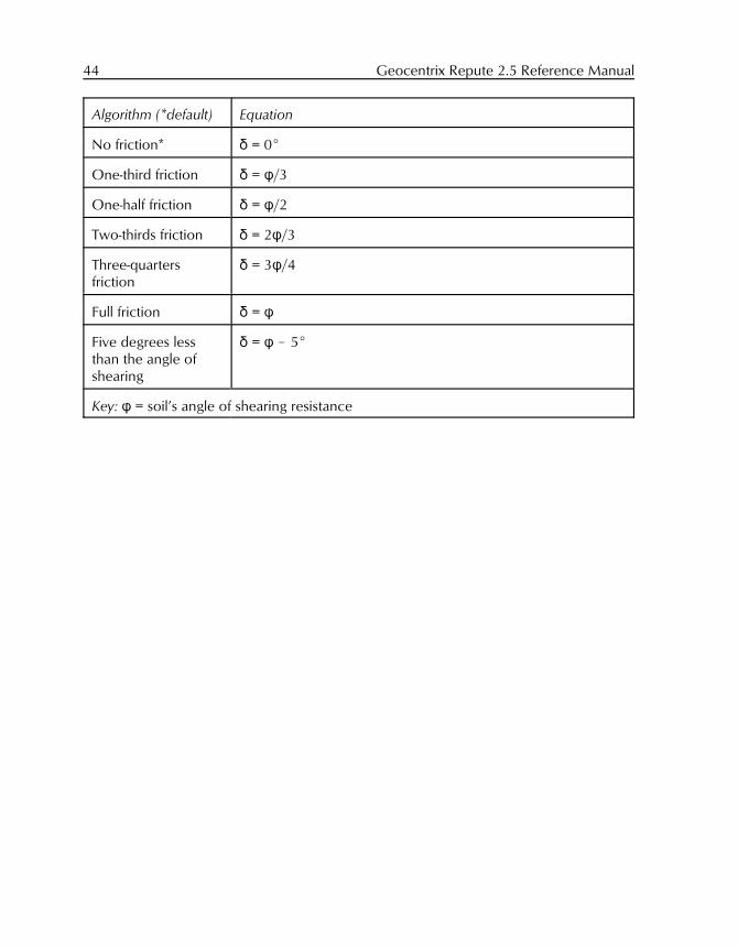
44 Geocentrix Repute 2.5 Reference Manual
Algorithm (*default) Equation
No friction* * = 0E
One-third friction * = n/3
One-half friction * = n/2
Two-thirds friction * = 2n/3
Three-quartersfriction
* = 3n/4
Full friction * = n
Five degrees lessthan the angle ofshearing
* = n ! 5E
Key: n = soil’s angle of shearing resistance
References 45
Chapter 7References
The following pages list the papers referred to throughout the main text of this manual.
46 Geocentrix Repute 2.5 Reference Manual
[1] Butterfield, R. and Banerjee, P. K. (1971), “The elastic analysis of compressible piles andpile groups”, Géotechnique 21, No. 1, 43-60.
[2] Basile, F. (1999), “Non-linear analysis of pile groups”, Proc Instn Civ Engng, GeotechEngng 137, No. 2, April, 105-115.
[3] Basile, F. (2003), “Analysis and design of pile groups”, in Numerical Analysis andModelling in Geomechanics (ed. J. W. Bull), Spon Press (Taylor & Francis Group Ltd), Oxford,Chapter 10, 278-315.
[4] Basile, F. (2010), “Torsional response of pile groups”, Proc. 11th DFI/EFFC Int. Conf. onGeotechnical Challenges in Urban Regeneration, London, 26-28 May 2010, 13pp.
[5] Mindlin, R. D. (1936), “Force at a point in the interior of a semi-infinite solid”, Physics 7,195-202.
[6] Poulos, H. G. (1979), “Settlement of single piles in nonhomogeneous soil”, J. Geotech.Engng, Am. Soc. Civ. Engrs 105, No. GT5, 627-641.
[7] Poulos, H. G. (1990), User's guide to program DEFPIG Deformation Analysis of PileGroups, Revision 6, School of Civil Engineering, University of Sydney.
[8] Leung, C. F. & Chow, Y. K. (1987), “Response of pile groups subjected to lateral loads”, Int. J. Numer. Anal. Meth. Geomechs 11, No. 3, 307-314.
[9] Chow, Y. K. (1986), “Analysis of vertically loaded pile groups”, Int. J. Numer. Anal. Meth.Geomechs 10, No. 1, 59-72.
[10] Chow, Y. K. (1987a), “Three-dimensional analysis of pile groups”, J. Geotech. Engng, Am.Soc. Civ. Engrs 113, No. 6, 637-651.
[11] Chow, Y. K. (1987), “Axial and lateral response of pile groups embedded innonhomogeneous soils”, Int. J. Numer. Anal. Meth. Geomechs 11, 621-638.
[12] Poulos, H. G. (1989), “Pile behaviour - theory and application”, 29th Rankine Lecture,Géotechnique 39, No. 3, 365-415.
[13] Yamashita, K., Tomono, M. & Kakurai, M. (1987), “A method for estimating immediatesettlement of piles and pile groups”, Soils and Fdns 27, No. 1, 61-76.
[14] Steinbrenner, W. (1934), Tafeln zur Setzungberechnung. Strasse 1, 221.
[15] Poulos, H. G. and Davis, E. H. (1980), Pile foundation analysis and design, New York:Wiley.
References 47
[16] Randolph, M. F. (1987), PIGLET, a computer program for the analysis and design of pilegroups.
[17] Broms, B. B. (1964), “Lateral resistance of piles in cohesive soils”, J. Soil Mechs FdnDivision, Am. Soc. Civ. Engrs 90, No. SM2, 27-63.
[18] Fleming, W. G. K., Weltman, A. J., Randolph, M. F., and Elson, W. K. (1992), PilingEngineering (2nd edn), Glasgow: Blackie Academic and Professional.
[19] Berezantzev, V. G., Khristoforov, V., and Golubkov, V. (1961), “Load bearing capacityand deformation of piled foundations”, Proc. 5th Int. Conf. Soil Mech. Fdn Engng, Paris 2,11-15.
[20] Poulos, H.G., and Bunce, G. (2008), "Foundation design for the Burj Dubai - TheWorld's Tallest Building", Proc. 6th Int. Conf. on Case Histories in Geotechnical Engineeringand Symposium in Honor of Professor James K. Mitchell, Arlington, VA (USA), Paper No.1.47, pp. 1-16.
[21] Poulos, H.G. (2016), "Tall building foundations: design methods and applications",Innov. Infrastruct. Solut. 1: 10. doi:10.1007/s41062-016-0010-2, 51p.
[22] Cox, W. R., Dixon, D. A., and Murphy, B. S. (1984), “Lateral load tests on 25.4-mm(1-in.) diameter piles in very soft clay in side-by-side and in-line groups”, Laterally loadeddeep foundations: analysis and performance, ASTM STP 835, J. A. Langer, E. T. Mosley, andC. D. Thompson (ed), American Society for Testing and Materials, 122-139.
[23] Brown, D. A. and Shie, C. F. (1990). “Numerical experiments into group effects on theresponse of piles to lateral loading”, Computers and Geotechnics 10, No. 4, 211-230.
[24] Ng, C. W. W., Zhang, L., and Nip, D. C. N. (2001), “Response of laterally loadedlarge-diameter bored pile groups”, J. Geotech. and Geoenv. Engng, Am. Soc. Civ. Engrs 127,No. 8, 658-669.
[25] Reese, L. C., Wang, S. T., Arrellaga, J. A., and Hendrix, J. (1996). Computer programGROUP for Windows user's manual, version 4.0. Ensoft, Inc., Austin, Texas.
[26] Duncan, J. M. and Chang, C. Y. (1970), “Non-linear analysis of stress and strain in soils”, J. Soil Mechs Fdn Division, Am. Soc. Civ. Engrs 96, No. SM5, 1629-1681.
[27] Randolph, M. F. (1994), “Design methods for pile groups and piled rafts”, Proc. 13th Int.Conf. Soil Mech. Fdn Engng, New Delhi 5, 61-82.
[28] Poulos, H. G. (1994), “Settlement prediction for driven piles and pile groups”, Proc.Conf. on vertical and horizontal deformations of foundations and embankments, CollegeStation, Texas, Geotechnical Special Publication, Vol. 2, No. 40, 1629-1649.
48 Geocentrix Repute 2.5 Reference Manual
[29] Fleming’s paper A new method for single pile settlement prediction and analysis (1992),Géotechnique, vol. 42, no. 3, pp 411-425.
[30] Fleming, Weltman, Randolph, and Elson (1992), Piling engineering (2nd
edition),Glasgow: Blackie Academic and Professional, pp. 122-140
[31] BS 8004: 1986, Code of practice for foundations, British Standards Institution, London.
[32] ENV 1997-1: 1994 (pre-standard), Eurocode 7: Geotechnical design – Part 1: Generalrules, European Committee for Standardization, Brussels.
[33] EN 1997-1: 2004, Eurocode 7: Geotechnical design – Part 1: General rules, EuropeanCommittee for Standardization, Brussels.
[34] UK National Annex to BS EN 1997-1: 2007, British Standards Institution, London.
[35] Irish National Annex to IS EN 1997-1: 2007, National Standards Authority of Ireland,Dublin.
[36] Norme tecniche per le costruzioni, DM 14/01/2008, Il Ministro delle Infrastrutture.
[37] Singapore National Annex to SS EN 1997-1: 2010, SPRING, Singapore.
[38] BS 8004: 1986, Code of practice for foundations, British Standards Institution, London.
[39] EN ISO 14688, Geotechnical investigation and testing — Identification and classificationof soil, European Committee for Standardization, Brussels.
[40] EN ISO 14689, Geotechnical investigation and testing — Identification and classificationof rock, European Committee for Standardization, Brussels.
[41] Terzaghi, K. and Peck, R. B. (1967), Soil mechanics in engineering practice (2ndedition), John Wiley & Sons, Inc, 729pp.
[42] NAVFAC DM-7 (1971), Naval Facilities Engineering Command,Virginia, USA.
[43] Winterkorn H.F. and Fang F.Y. (1975), Foundation Engineering Handbook, Springer.
[44] Canadian Foundation Engineering Manual (1978), Canadian Geotechnical Society.
[45] Reynolds C.E. and Steedman J. (1981), Reinforced Concrete Designers’ Manual.
[46] Bell F.G. (1983), Engineering properties of soils and rocks (2nd
edition), Butterworths,London, 149pp.
References 49
[47] Mitchell R.J. (1983), Earth structures engineering, Allen & Unwin Inc., Boston.
[48] TradeARBED's Spundwand-Handbuch Teil 1, Grundlagen (1986)
[49] Bolton, M. D. (1986) A guide to soil mechanics.
[50] Clayton C.R.I. and Militiski J. (1986), Earth pressure and earth-retaining structures, SurreyUniversity Press, Glasgow and London, 300pp.
[51] Clayton C.R.I. (1989), The mechanical properties of the Chalk, Proc. Int. Chalk Symp.,Brighton.
[52] Tomlinson M.J. (1995), Foundation design and construction (6th edition), Longman
Scientific & Technical, Harlow, Essex, 536pp.
[53] British Steel's Piling Handbook (1997)
[54] EN 206-1, Concrete. Specification, performance, production and conformity, EuropeanCommittee for Standardization, Brussels.
[55] Arya C. (1994), Design of structural elements, E &FN Spon.
[56] EN 1992-1-1, Eurocode 2: Design of concrete structures – Part 1-1 General rules andrules for buildings, European Committee for Standardization, Brussels.
[57] Fleming, Weltman, Randolph, and Elson (1992) Piling engineering (2nd
edition),Glasgow: Blackie Academic and Professional, 390pp.
[58] EN 1993-1-1, Eurocode 3: Design of steel structures – Part 1-1 General rules and rulesfor buildings, European Committee for Standardization, Brussels.
[59] EN 1993-1-1 (loc. cit.).
[60] Skempton A.W. (1959), “Cast in-situ bored piles in London Clay”, Géotechnique, Vol.9, pp153-173.
[61] Randolph, M.F., and Murphy, B.J. (1985), “Shaft capacity of driven piles in clay”, Proc.17
th Offshore Technology Conf., Houston, Texas, Vol. 1, pp371-378 (Paper OTC 4883).
[62] Semple, R.M., and Rigden, W.J. (1984), “Shaft capacity of driven pile in clay”, Analysisand design of pile foundations, ASCE, October, pp59-79.
[63] Bowles, J.E. (1997), Foundation analysis and design (5th edition), New York: McGraw
Hill, 1175pp.
50 Geocentrix Repute 2.5 Reference Manual
[64] Sladen J.A. (1992), “The adhesion factor: applications and limitations”, Can. Geotech.J. Vol. 29, pp322-326.
[65] O’Neill, M.W, and Reese, L.C. (1999), Drilled shafts: construction procedures and designmethods, Report No. FHWA-IF-99-025, Washington: US Dept of Transportation, FederalHighway Administration, 790pp.
[66] US Army Corps of Engineers (1991), Design of pile foundations, Engineer Manual No1100-2-2906, Honolulu: University Press of the Pacific, c171pp.
[67] Terzaghi, K. (1943), Theoretical soil mechanics, New York: Wiley.
[68] Meyerhof, G. G. (1963) ‘Some recent research on the bearing capacity of foundations’,Can. Geotech. J., 1(1), pp. 16–26.
[69] Brinch-Hansen, J. (1970) A revised and extended formula for bearing capacity, DanishGeotechnical Institute, Bulletin No. 28, 6pp.
[70] Vesic, A. S. (1973) ‘Analysis of ultimate loads of shallow foundations’, J. Soil Mech.Found. Div., Am. Soc. Civ. Engrs, 99(1), pp. 45–73.
[71] Berezantsev V.G., Kristoforov V., and Golubkov V. (1961), “Load bearing capacity anddeformation of pile foundations”, Proc. 5
th Int. Conf. Soil Mech. And Fdn Engng, Vol 2, pp11-
15.
[72] Spangler M.G. and Handy R.L. (1982), Soil Engineering, HarperCollins.
[73] API RP2A, Recommended Practice for Planning, Designing and Constructing FixedOffshore Platforms — Working Stress Design.
[74] EN 1997-1, (loc. cit.).
[75] Zhu, F., Clark, J. I., and Phillips, R. (2001), “Scale effect of strip and circular Footingsresting on a dense sand”, J. Geotech. Geoenviron. Eng., 127(7), 613–621.
[76] O’Neill M. and Reese L.C. (1999), Drilled shafts: Construction procedures and designmethods, Federal Highways Administration.
[77] Rollins K.M., Clayton R.J., and Mikesell R.C. (1997), “Ultimate side friction of drilledshafts in gravels”, Foundation Drilling, Vol. 36, No 5, Association of Drilled Shaft Engineers,Dallas, Texas, USA.
[78] Rollins et al. (loc. cit.).

References 51
[79] Bhushan K. (1982), Discussion of “New design correlations for piles in sand”, J. Geotec.Engng. Div., ASCE, Vol. 108, GT11, pp1500-1501.
[80] API RP2A, (loc. cit.).
[81] NHBC (1992), National House-Building Council Standards: Vol 1.