geochemical phase diagrams and gale diagramsreiner/papers/geology.pdfa geochemistry-discrete...

GEOCHEMICAL PHASE DIAGRAMS AND GALE

DIAGRAMS

P.H. EDELMAN, S.W. PETERSON, V. REINER, AND J.H. STOUT

Abstract. The problem of predicting the possible topologies ofa geochemical phase diagram, based on the chemical formula ofthe phases involved, is shown to be intimately connected with andaided by well-studied notions in discrete geometry: Gale diagrams,triangulations, secondary fans, and oriented matroids.

Contents

1. Introduction 22. A geochemistry-discrete geometry dictionary 63. Chemical composition space 64. Triangulations and subdivisions 105. Secondary fans 136. Gale diagrams and duality 177. Geometry of the phase diagram in general 217.1. Bistellar operations and 1-dimensional stability fields 237.2. Invariant points and indifferent crossings 258. The case m = n + 2: phase diagram = Gale diagram 289. The case m = n + 3: phase diagram = affine Gale diagram 309.1. The spherical representation: closed nets 319.2. Two-dimensional affine Gale diagrams 3310. Further implications/applications 3510.1. Slopes around invariant points 3510.2. Counting potential solutions 37References 40

1991 Mathematics Subject Classification. 52B35, 52C40, 86A99.Key words and phrases. Gale diagram, Gale transform, phase diagram, trian-

gulation, secondary polytope, secondary fan, geochemistry, heterogeneous equilib-rium, closed net, Euler sphere.

Work of second author was carried out partly as a Masters Thesis at the Uni-versity of Minnesota Center for Industrial Mathematics, and partly supported bya University of Minnesota Grant-in-Aid of Research. Third author was partiallysupported by NSF grant DMS–9877047.

1

2 P.H. EDELMAN, S.W. PETERSON, V. REINER, AND J.H. STOUT

Temperature ( C)o

Ice

Water

Triple Point

icew

ater water

steam

Steam

100

1

Pres

sure

(ba

r)

steamice

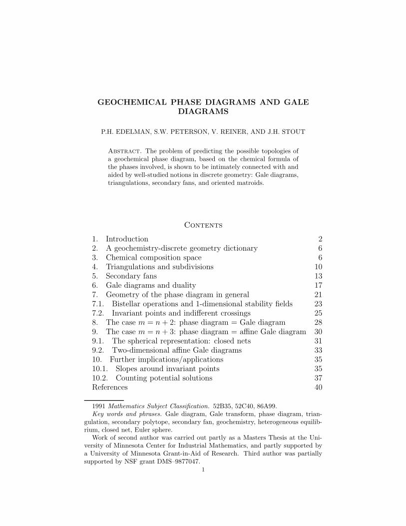
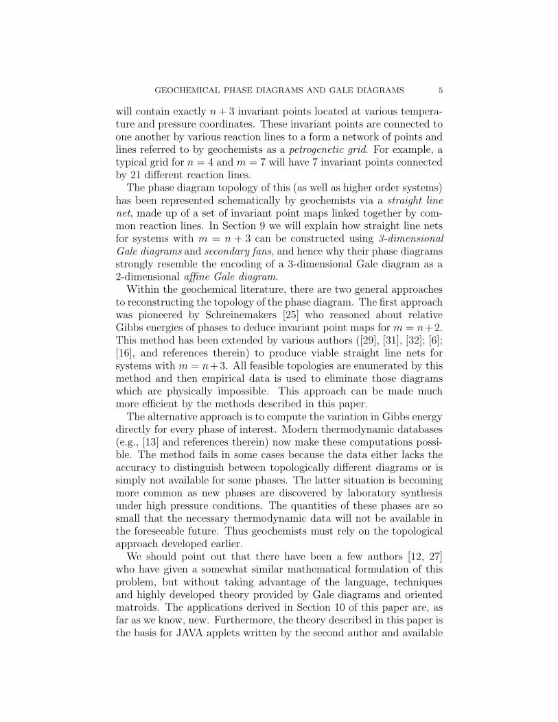
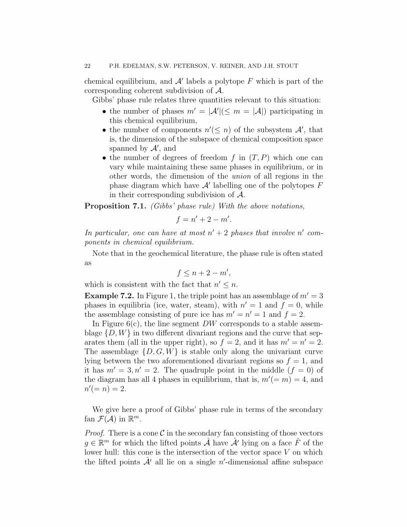
Figure 1. The phase diagram for the simple chemicalsystem with phases ice, water, and steam.

1. Introduction

A central problem in geochemistry has been to understand how theequilibrium state of a chemical system varies with temperature andpressure, and predict the form of its temperature-pressure phase dia-gram (hereafter called just the phase diagram). The purpose of thispaper is to explain how some recently developed tools from discretegeometry (the theory of oriented matroids, triangulations, Gale dia-grams, and secondary fans) can be used to elucidate this problem. Ourgoal is to be comprehensible to both discrete geometers and workers ingeochemistry.

Figure 1 illustrates the familiar phase diagram for a simple chemi-cal system that involves three phases (ice, water, steam) of the samechemical compound, H2O. The topological structure of this diagramis fairly simple: there is a unique point, called a triple point, where allthree phases can be present in equilibrium. The triple point lies at thejunction of three curves. Along each of these curves exactly two of thephases are present in equilibrium (either ice + water, or ice + steam,or water + steam), and these three curves separate two-dimensional

GEOCHEMICAL PHASE DIAGRAMS AND GALE DIAGRAMS 3

regions where only one phase (pure ice, or pure water, or pure steam)can be present in equilibrium.

This example of a phase diagram is quite an elementary one, inthat all the phases have the same underlying chemistry, that of H2O.Geochemists are interested in phase diagrams as the principal tool inreconstructing the temperature and pressure conditions from rock for-mations once deep within the Earth but which now reside at its surface.Thus it is important to have accurate phase diagrams involving muchmore complex systems in which the phases have different chemistry aswell as different states.

To be more precise, a phase means a physically homogeneous sub-stance, having its own chemical formula, although different phaseswithin the system can have the same formula (as in the ice-water-steamexample). At a particular temperature and pressure, the equilibriumstate consists of groups of one or more phases that are referred to asphase assemblages. Within a closed system at fixed temperature andpressure, only certain phase assemblages will be stable, namely thosehaving the lowest possible Gibbs free energy under the given condi-tions. Other assemblages with higher energy than the minimum underthose conditions are referred to as metastable – these assemblages reactspontaneously to produce a stable assemblage and a net decrease inenergy. For example, pure water placed in the stability field of ice willspontaneously freeze because a lower Gibbs energy assemblage (ice) isavailable under those conditions. When there are different chemicalformulae present among the phases, more exotic reactions than simplephase changes are possible. The regions of simultaneous stability forvarious collections of phase assemblages, and the chemical reactionsthat relate them are conveniently summarized in the phase diagram.

The locus of temperatures and pressures within which a particularphase assemblage is stable is called its stability field. The stabilityfield is called invariant, univariant, or divariant depending upon itsdimension, that is, the number of degrees of freedom one can varywhile staying within that stability field. In the example above, thetriple point (ice-water-steam) is an invariant point, there are three uni-variant curves (ice-water, ice-steam, water-steam), and three divariantstability fields (pure ice, pure water, pure steam). The univariant fieldscorrespond to simple chemical reactions that transform one phase as-semblage to another, and hence are sometimes referred to as reactionlines. In producing these phase diagrams, a prediction of the possi-ble topologies (i.e. number of invariant points, number of univariantcurves joining them, etc.) is indispensable, as the thermodynamic data


needed to resolve such topological features can sometimes be difficultto obtain.

It turns out that much of the complexity of the phase diagram for achemical system is governed by two parameters:

• the number of phases, m, and• the number of components, n (defined below).

We will see in Section 3 that these two parameters correspond to thesize of the ground set and the rank of a related vector configuration(or affine point configuration, or oriented matroid) associated with thechemical system. It is well-known, in both geochemistry and discretegeometry, that what matters most in predicting the complexity of thephase diagram is not the sizes of n and m, but rather the sizes of nand m − n (the rank and the co-rank).

The number of components n for a chemical system is defined asfollows. Think of the chemical formulae of the various phases of thesystem as vectors in a vector space of all possible such formulae (thechemical composition space– see Section 3), whose coordinate axes cor-respond to the elements present on Earth. Then the number n of com-ponents of the chemical system is simply the dimension of the subspacespanned by the chemical formulae of the phases present in the system1.For example, the system of ice, water and steam from Figure 1 hasm = 3 phases and n = 1, while the system depicted in Figure 2 hasm = 4 phases and n = 2.

Phase diagram topologies for chemical systems with m ≤ n + 2 arefairly well-understood, even as m grows large. For m ≤ n + 1 they areessentially trivial, and for m = n + 2, they look roughly like Figure 1,having an invariant point surrounded by several univariant reactioncurves. The schematic picture of such an invariant point surroundedby reaction curves is referred to as an invariant point map [17]. Wewill explain in Section 8 why invariant point maps look roughly like atwo-dimensional Gale diagram, in concordance with rules for the phasediagram’s construction first delineated by Schreinemakers [25] nearly100 years ago.

However, by m = n + 3 (a situation common for chemical systemsapplicable to the Earth) the topology of the phase diagram can becomequite complex as m grows large. For example, under certain genericityassumptions about the chemical formulae of the phases, the diagram

1It will be convenient in Section 3 to choose a basis for this space, that is a mini-mal set of phases such that all the formulae of the phases can be expressed as linearcombinations of these basic components; hence the term number of components ofthe system.


will contain exactly n + 3 invariant points located at various tempera-ture and pressure coordinates. These invariant points are connected toone another by various reaction lines to a form a network of points andlines referred to by geochemists as a petrogenetic grid. For example, atypical grid for n = 4 and m = 7 will have 7 invariant points connectedby 21 different reaction lines.

The phase diagram topology of this (as well as higher order systems)has been represented schematically by geochemists via a straight linenet, made up of a set of invariant point maps linked together by com-mon reaction lines. In Section 9 we will explain how straight line netsfor systems with m = n + 3 can be constructed using 3-dimensionalGale diagrams and secondary fans, and hence why their phase diagramsstrongly resemble the encoding of a 3-dimensional Gale diagram as a2-dimensional affine Gale diagram.

Within the geochemical literature, there are two general approachesto reconstructing the topology of the phase diagram. The first approachwas pioneered by Schreinemakers [25] who reasoned about relativeGibbs energies of phases to deduce invariant point maps for m = n+2.This method has been extended by various authors ([29], [31], [32]; [6];[16], and references therein) to produce viable straight line nets forsystems with m = n+3. All feasible topologies are enumerated by thismethod and then empirical data is used to eliminate those diagramswhich are physically impossible. This approach can be made muchmore efficient by the methods described in this paper.

The alternative approach is to compute the variation in Gibbs energydirectly for every phase of interest. Modern thermodynamic databases(e.g., [13] and references therein) now make these computations possi-ble. The method fails in some cases because the data either lacks theaccuracy to distinguish between topologically different diagrams or issimply not available for some phases. The latter situation is becomingmore common as new phases are discovered by laboratory synthesisunder high pressure conditions. The quantities of these phases are sosmall that the necessary thermodynamic data will not be available inthe foreseeable future. Thus geochemists must rely on the topologicalapproach developed earlier.

We should point out that there have been a few authors [12, 27]who have given a somewhat similar mathematical formulation of thisproblem, but without taking advantage of the language, techniquesand highly developed theory provided by Gale diagrams and orientedmatroids. The applications derived in Section 10 of this paper are, asfar as we know, new. Furthermore, the theory described in this paper isthe basis for JAVA applets written by the second author and available


on the web [18], which give practical tools for use in geochemistry topredict phase diagram topology.

2. A geochemistry-discrete geometry dictionary

For the convenience of the reader, and as a guide to what lies instore, we present a (very rough) dictionary of corresponding terms.

Geochemistry Discrete geometry

chemical formula for a phase vector in composition spacechemical system acyclic vector configuration Vchemography affine point configuration Anumber of phases m number of vectors/pointsnumber of components n rank of vector/point configurationreactions among phases linear/affine dependences of V/Aminimal reactions circuitsstable assemblage of phases simplex in a triangulation of Aphase diagram affine plane slice of secondary fanphase diagram when m = n + 2 2−dimensional Gale diagram A∗

reaction half-line for m = n + 2 vector in 2−dim’l Gale diagram A∗

phase diagram when m = n + 3 2−dim’l affine Gale diagram for A∗

invariant point when m = n + 3 vector in 3−dim’l Gale diagram A∗

closed net when m = n + 3 spherical representation of A∗

Euler sphere for m = n + 3 great circles normal to A∗

3. Chemical composition space

In this section, we introduce the chemical composition space thatallows one to associate to each chemical system a configuration of vec-tors, an affine point configuration, and their oriented matroid. For ter-minology on vector configurations, point configurations and orientedmatroids, we refer the reader to two excellent references: the bible ofthe subject [2] (in particular, its §1.2), and Ziegler’s book [33, Lecture6].

Definition 3.1. The formulae of chemical compounds may be repre-sented in a natural way by vectors in a chemical composition spacewhose axes are indexed by the elements in the periodic table. For ex-ample, H2O has coordinates which are two units on the hydrogen axis,one unit on the oxygen axis, and zero on all other axes. The m phases ofa chemical system in this way give rise to a collection V = {v1, . . . , vm}of vectors spanning a subspace of some dimension n, which is calledthe number of components of the system. By picking a basis for this


12

WG

DC

(x)=1

W G D C

(a) (b)

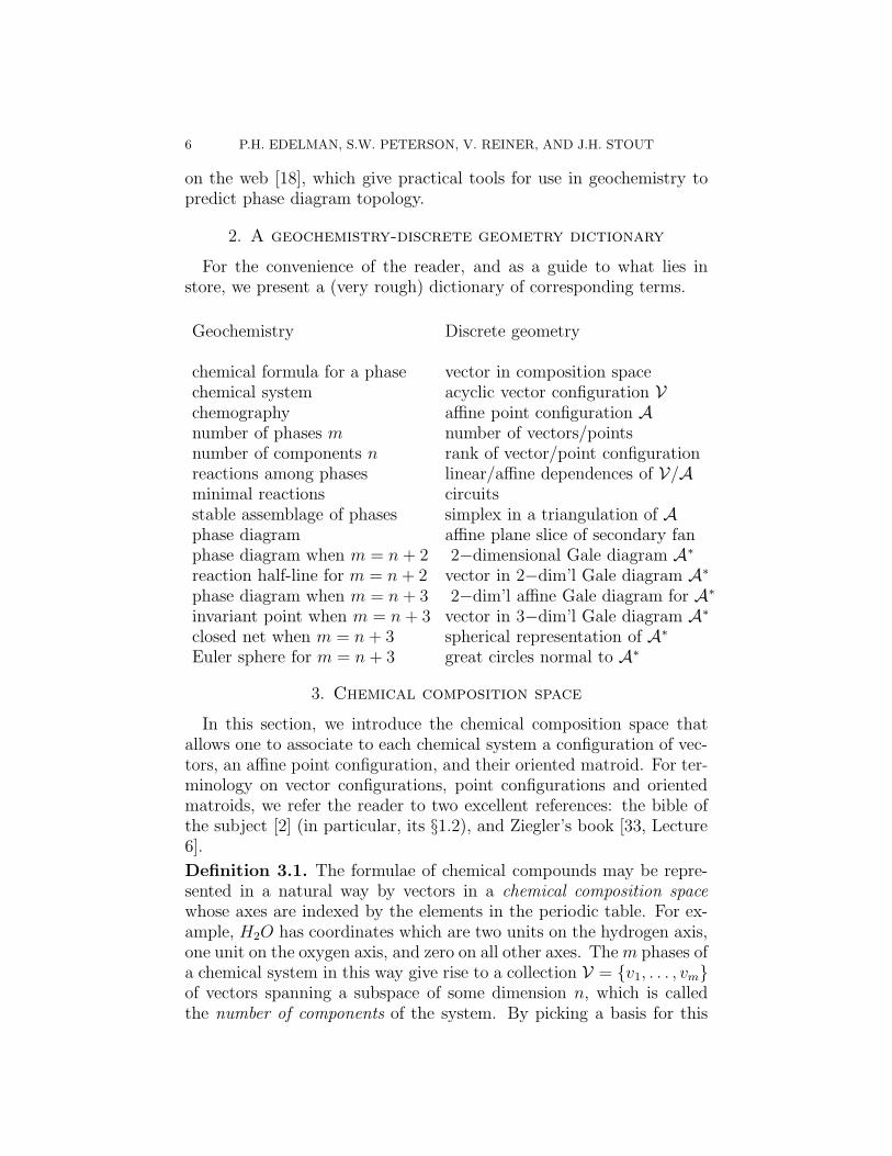
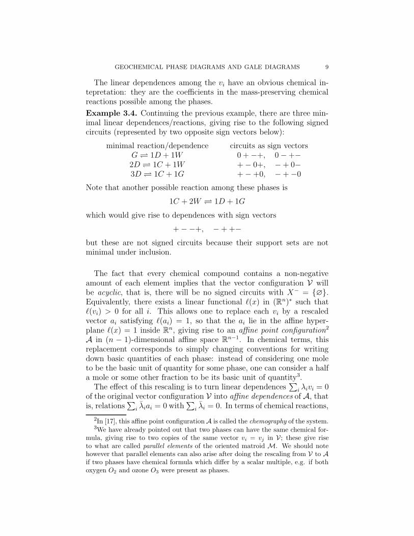
Figure 2. (a) Vector configuration V, and (b) affinepoint configuration A for the chemical system withphases corundum (C), diaspore (D), gibbsite (G), andwater (W).

subspace, we can identify it with Rn and specify each vi by a column

vector in Rn. This allows us to identify V with an n×m matrix having

full rank n, which we also call V by an abuse of notation.

Example 3.2. Consider a chemical system of relevance to geologyhaving m = 4 phases, which we denote by descriptive initials ratherthan v1, v2, v3, v4:

(1)

C = corundum Al2O3

D = diaspore AlO(OH)G = gibbsite Al(OH)3

W = water H2O.

Since the compounds in this system involve only the elements Al, O, H,this system can have n at most 3. But one can check that these chemicalformulae span a space of dimension n = 2. Choosing C and W to bethe standard basis vectors in this space (that is, the components forthis system), one can represent the configuration V as the columns of


the following matrix

(2)

C D G W

V =

[

1 12

12

00 1

232

1

]

and the associated vector configuration is depicted in Figure 2(a).

Notice that by choosing a basis that identifies this n-dimensionalsubspace with R

n, we are already abstracting away from the actualchemical formulae of the phases and paying attention only to propertiesthat are invariant under a simultaneous change-of-basis acting on thevectors, that is, properties invariant under GLn(R). One such set ofproperties is the oriented matroid associated to the vector configurationV.

Definition 3.3. The oriented matroid M associated to V is a combi-natorial abstraction of the vectors V which forgets their actual coor-dinates, but retains data specifying the signs involved in linear depen-dences among the vi. The way in which we choose to record this data isto list the signed circuits of M coming from each minimal (non-trivial)linear dependence

∑

i λivi = 0, that is, the signed set (X+, X−) where

X± := {i ∈ {1, . . . , m} : sign(λi) = ±}.

Here minimality for signed sets is interpreted with respect to the or-dering of their support sets:

(X+, X−) < (Y +, Y −) means X+ ∪ X− ⊆ Y + ∪ Y −.

It is sometimes convenient to represent a signed set (X+, X−) insteadby its sign vector in {+, 0,−}m which has ± in the coordinates indexedby X±, and 0 in all other coordinates. For example, a minimal depen-dence of the form +5v1 − 3v2 + 7

8v4 among m = 4 phases would be

recorded by the circuit whose signed set is ({1, 4}, {2}) or by its signvector (+ − 0+).

It is possible to write down a small set of circuit axioms satisfied byby the set C of signed circuits coming from any vector configuration,in such a way that collections of signed sets satisfying these axioms(oriented matroids) mimic many features of sets of vectors in a realvector space– see [2, p. 4]. Note that since the negation of a lineardependence gives another linear dependence, one of these circuit axiomsfor an oriented matroid says that the set of sign vectors of circuits isclosed under negation.


The linear dependences among the vi have an obvious chemical in-tepretation: they are the coefficients in the mass-preserving chemicalreactions possible among the phases.

Example 3.4. Continuing the previous example, there are three min-imal linear dependences/reactions, giving rise to the following signedcircuits (represented by two opposite sign vectors below):

minimal reaction/dependence circuits as sign vectorsG 1D + 1W 0 + −+, 0 − +−2D 1C + 1W + − 0+, − + 0−3D 1C + 1G + − +0, − + −0

Note that another possible reaction among these phases is

1C + 2W 1D + 1G

which would give rise to dependences with sign vectors

+ −−+, − + +−

but these are not signed circuits because their support sets are notminimal under inclusion.

The fact that every chemical compound contains a non-negativeamount of each element implies that the vector configuration V willbe acyclic, that is, there will be no signed circuits with X− = {∅}.Equivalently, there exists a linear functional `(x) in (Rn)∗ such that`(vi) > 0 for all i. This allows one to replace each vi by a rescaledvector ai satisfying `(ai) = 1, so that the ai lie in the affine hyper-plane `(x) = 1 inside R

n, giving rise to an affine point configuration2

A in (n − 1)-dimensional affine space Rn−1. In chemical terms, this

replacement corresponds to simply changing conventions for writingdown basic quantities of each phase: instead of considering one moleto be the basic unit of quantity for some phase, one can consider a halfa mole or some other fraction to be its basic unit of quantity3.

The effect of this rescaling is to turn linear dependences∑

i λivi = 0of the original vector configuration V into affine dependences of A, thatis, relations

∑

i λiai = 0 with∑

i λi = 0. In terms of chemical reactions,

2In [17], this affine point configuration A is called the chemography of the system.3We have already pointed out that two phases can have the same chemical for-

mula, giving rise to two copies of the same vector vi = vj in V ; these give riseto what are called parallel elements of the oriented matroid M. We should notehowever that parallel elements can also arise after doing the rescaling from V to Aif two phases have chemical formula which differ by a scalar multiple, e.g. if bothoxygen O2 and ozone O3 were present as phases.


this means that the reactions will not only achieve mass-balance foreach atom, but also “coefficient balance”, as in the following example.

Example 3.5. Continuing the previous example, we can choose thelinear function `(x) = x1 + x2 in R

2 and rescale the coordinates ofC, D, G, W so that they have `(x) = 1, giving the new matrix

(3)

C D 12G W

A =

[

1 12

14

00 1

234

1

]

The affine point configuration in R1 represented by A is depicted in

Figure 2 (b).The rescaling in this case only required replacing G by 1

2G, so that,

for example the previous reaction/linear dependence

1G 1D + 1W

1Al(OH)3 1AlO(OH) + 1H2O

which achieves mass-balance for each atom but not coefficient balance(1 6= 1 + 1), now gives rise to the affine dependence

2 ·

(

1

2G

)

1D + 1W,

achieving coefficient balance: 2 = 1 + 1.

Switching from the vector configuration V to the affine point config-uration has psychological advantages, in that it allows one to reducethe dimension by one for visualization purposes, and it makes it easierto think about our next topic: triangulations4 of A.

4. Triangulations and subdivisions

Our goal in this section is to explain a phenomenon well-known togeochemists: by performing reactions that minimize the Gibbs free en-ergy resulting in a stable phase assemblage at a particular temperatureand pressure, Nature (generically) “computes” a triangulation of thepoint set A.

Having fixed a temperature and pressure (T, P ), each of the phasesa1, . . . , am of the chemical system will have a certain Gibbs free energy

4We should point out that there is a well-defined notion of triangulations forgeneral vector configurations (even when they are not acyclically oriented), as wellas for oriented matroids that do not come from configurations of vectors. See [24]and the references contained therein.


12

1212

12W G D C

gW(T,P)

gC(T,P)

gD(T,P)

gG

(T,P)

W D CG

(a) (b)

W

G

D

C

W

GD

C

^

Gibbsenergy

^

^^ ^

^^

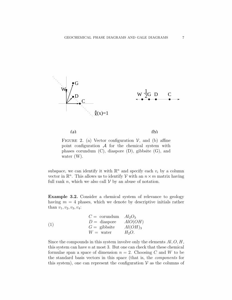
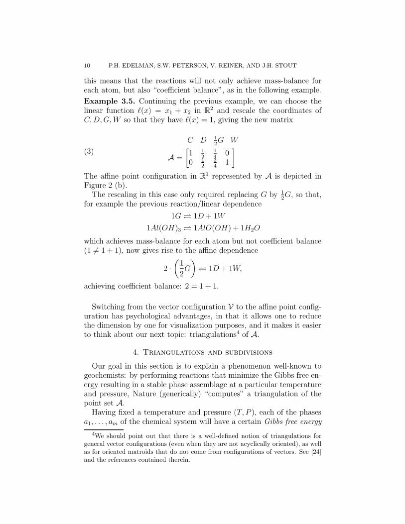
Figure 3. The chemography A from Figure 2, “lifted”to A by the Gibbs energy values at two different valuesof temperature and pressure.

gi(T, P ) per molar quantity (or per whatever basic quantity is beingused after rescaling vi to ai).

Definition 4.1. These values gi(T, P ) can be used as heights to “lift”the points ai in R

n−1 to points

ai :=

[

ai

gi(T, P )

]

∈ Rn,

giving a new lifted configuration of points A. In other words, we plotthe points ai together with their height along an extra Gibbs energyaxis; see Figure 3 for two examples having n = 2.

The convex hull, that is the set of all convex combinations, of this setA of lifted points has the following physical interpretation. Supposewe have an assemblage consisting of xi units of the basic quantity ofphase ai for each i = 1, . . . , m, and assume (without loss of generality)that

∑

i xi = 1. Then this assemblage will have total Gibbs energy∑

i xigi(T, P ), which is the same as the height on the Gibbs energy axis


of the point∑

i xiai which is a weighted average of the lifted points A,and therefore lies somewhere in their convex hull. If this point doesnot lie on the lower convex hull of these lifted points, then this is nota stable assemblage of phases: there exist some reaction(s) availablewhich would alter the fractions of each phase ai in a way that lowersthe total Gibbs energy.

Example 4.2. We continue our previous example, and assume that theGibbs energies of the phases are as depicted in Figure 3(a). Considerthe assemblage consisting of 1

2mole of C together with 1

2mole of D.

It lifts to the point 12C + 1

2D at the midpoint of the line segment CD

in Figure 3(a), whose height 12gC(T0, P0) + 1

2gD(T0, P0) represents the

total Gibbs energy of this assemblage. It is not stable because one canrun the reaction

3D � 1C + 1G

in the forward direction to convert the 12

mole of D into 16

mole eachof C and G. This creates an assemblage with lower total Gibbs energyconsisting of 2

3mole of C together with 1

6mole of G (or equivalently,

13

mole of 12G). The latter assemblage however is stable, as it lifts to a

point on the segment CG lying in the lower convex hull of A.On the other hand, if the Gibbs energies of the phases looked as they

do in Figure 3(b), then the initial assemblage of 12

mole of C together

with 12

mole of D would have been stable, and no reactions would occur.

Note that even after the temperature and pressure (T, P ) have beenfixed, there can be more than one possible stable assemblage, and whichstable assemblages appear depends upon the initial quantities of eachphase present. In petrology, when one takes various samples from dif-ferent locations inside a stratum of rock formed under the same tem-perature and pressure conditions, one has a chance of sampling fromall the different stable assemblages.

From the previous discussion, we conclude that the sets of phaseswhich can form stable assemblages correspond to the sets of verticeswhich lie on a face of the lower convex hull of A. Note that projectingthese faces of the lower hull in R

n down into Rn−1 produces a set of

convex polytopes that disjointly cover the convex hull of A, formingwhat is usually called a polytopal subdivision of A. If the vector

g = (g1(T, P ), . . . , gm(T, P )) ∈ Rm

is sufficiently generic, then each of the faces of the lower convex hullwill be an (n − 1)-dimensional simplex (that is, the convex hull of n


affinely independent points), and this polytopal subdivision is called atriangulation of A; see [10, Chapter 7] for formal definitions.

Definition 4.3. Triangulations and polytopal subdivisions of A whichare induced in this fashion from a vector of heights g = (g1, . . . , gm)in R

m are called coherent or regular, and we call ∆(g) the subdivisioninduced by g.

We summarize here some of the conclusions of the preceding discus-sion.

Proposition 4.4. For each fixed temperature and pressure (T, P ), thevector

g = g(T, P ) := (g1(T, P ), . . . , gm(T, P )) ∈ Rm

of Gibbs energies for the phases A = {a1, . . . , am} induces a coherentpolytopal subdivision ∆(g) of A.

The polytopes participating in this subdivision have vertex sets corre-sponding exactly to the stable assemblages of phases at that temperatureand pressure (T, P ).

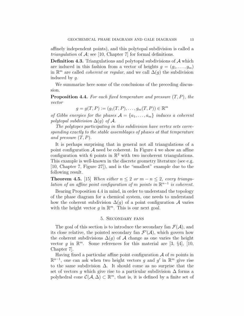
It is perhaps surprising that in general not all triangulations of apoint configuration A need be coherent. In Figure 4 we show an affineconfiguration with 6 points in R

2 with two incoherent triangulations.This example is well-known in the discrete geometry literature (see e.g.[10, Chapter 7, Figure 27]), and is the “smallest” example due to thefollowing result.

Theorem 4.5. [15] When either n ≤ 2 or m − n ≤ 2, every triangu-lation of an affine point configuration of m points in R

n−1 is coherent.

Bearing Proposition 4.4 in mind, in order to understand the topologyof the phase diagram for a chemical system, one needs to understandhow the coherent subdivision ∆(g) of a point configuration A varieswith the height vector g in R

m. This is our next goal.

5. Secondary fans

The goal of this section is to introduce the secondary fan F(A), andits close relative, the pointed secondary fan F ′(A), which govern howthe coherent subdivisions ∆(g) of A change as one varies the heightvector g in R

m. Some references for this material are [3, §4], [10,Chapter 7].

Having fixed a particular affine point configuration A of m points inR

n−1, one can ask when two height vectors g and g′ in Rm give rise

to the same subdivision ∆. It should come as no surprise that theset of vectors g which give rise to a particular subdivision ∆ forms apolyhedral cone C(A, ∆) ⊂ R

m, that is, it is defined by a finite set of


Figure 4. Incoherent triangulations of an affine pointconfiguration A: the standard, smallest example, alongwith its two incoherent triangulations.

linear inequalities (which depend on the coordinates of the points Aand on ∆). As one varies the subdivision ∆, these cones C(A, ∆) fittogether to disjointly cover R

m.

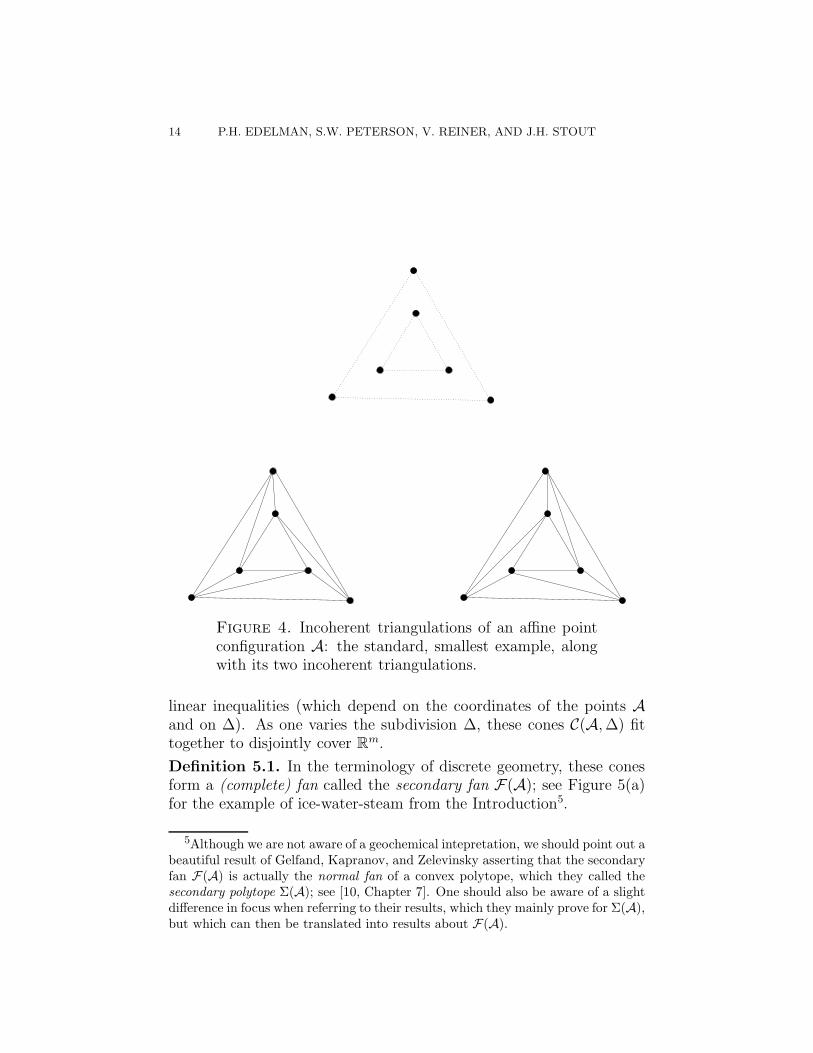
Definition 5.1. In the terminology of discrete geometry, these conesform a (complete) fan called the secondary fan F(A); see Figure 5(a)for the example of ice-water-steam from the Introduction5.

5Although we are not aware of a geochemical intepretation, we should point out abeautiful result of Gelfand, Kapranov, and Zelevinsky asserting that the secondaryfan F(A) is actually the normal fan of a convex polytope, which they called thesecondary polytope Σ(A); see [10, Chapter 7]. One should also be aware of a slightdifference in focus when referring to their results, which they mainly prove for Σ(A),but which can then be translated into results about F(A).


T

P

F(A)Row(A)

(a)

(b)

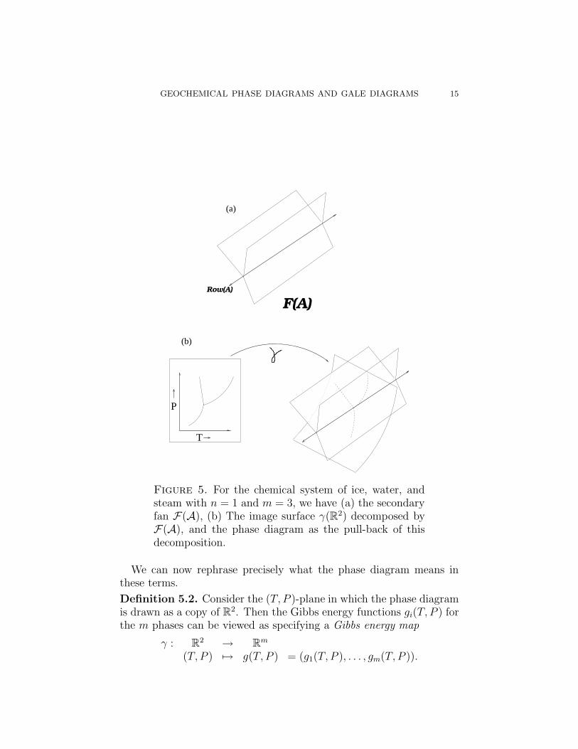
Figure 5. For the chemical system of ice, water, andsteam with n = 1 and m = 3, we have (a) the secondaryfan F(A), (b) The image surface γ(R2) decomposed byF(A), and the phase diagram as the pull-back of thisdecomposition.

We can now rephrase precisely what the phase diagram means inthese terms.

Definition 5.2. Consider the (T, P )-plane in which the phase diagramis drawn as a copy of R

2. Then the Gibbs energy functions gi(T, P ) forthe m phases can be viewed as specifying a Gibbs energy map

γ : R2 → R

m

(T, P ) 7→ g(T, P ) = (g1(T, P ), . . . , gm(T, P )).


The image γ(R2) of this map will be some 2-dimensional surface in Rm.

The decomposition of Rm into the cones of the secondary fan F(A) will

restrict to a decomposition of this surface γ(R2); see Figure 5(b) forthe example of ice-water-steam. This decomposition of the surface thenpulls back to induce a decomposition of the (T, P )-plane R

2 into regions,which are the regions of simultaneous stability for various collections ofphase assemblages (i.e. two pairs (T, P ), (T ′, P ′) lie in the same regionof the phase diagram if and only if their images under γ lie in thesame cone of F(A)). In other words, we have the following statement,illustrated in Figure 5(b):

Proposition 5.3. The phase diagram for a chemical system havingchemography A is exactly the decomposition of the (T, P )-plane R

2

which is the pull-back under γ−1 of the decomposition of the imagesurface γ(R2) induced by the cones of the secondary fan F(A).

Thus understanding possible phase diagram topologies amounts to un-derstanding the structure of the secondary fan F(A) and the Gibbsenergy map γ well enough to predict how the fan F(A) can decompose2-dimensional surfaces γ(R2) in R

m.It turns out that there is a natural way to cut down the dimension

of F(A) by the number of components n, without losing any informa-tion. Recall that A also denotes the n × m matrix whose columns arethe n-vectors ai (with each of these column vectors lying in the affinehyperplane `(x) = 1). It is not hard to see that two height vectors gand g′ which differ by a vector lying in the row space Row(A) of thismatrix A will induce the same coherent subdivision ∆: one can showthat the two configurations of lifted points they produce will differ byan affine transformation of R

n, and consequently their convex hulls willdiffer only by a “tilt” that does not affect the structure of their lowerhulls. As a consequence, each of the cones C(A, ∆) in the secondaryfan F(A) extends trivially in the n directions defined by Row(A); it isa Cartesian product

C(A, ∆) = C ′(A, ∆) × Row(A)

where C ′(A, ∆) is a cone in an (m − n)-dimensional subspace of Rm

complementary6 to Row(A). As ∆ varies over all coherent subdivi-sions, these cones C ′(A, ∆) disjointly cover this complementary (m−n)-dimensional subspace, producing what is called the pointed secondaryfan F ′(A).

6It would be more natural to think of the cones C ′(A, ∆) as living in the quotient

space Rm/Row(A), but we won’t quibble here


We next make explicit the simplifying assumption which is implicitin the geochemical literature on this subject.

Geochemical assumption 5.4. Over the ranges of temperature andpressure (T, P ) ∈ R

2 relevant to most phase diagrams, the Gibbs energymap γ : R

2 → Rm is sufficiently close to linear that the image surface

γ(R2) behaves nearly like a 2-dimensional affine plane in Rm.

Furthermore, this 2-dimensional affine plane is located genericallywith respect to the cones of the secondary fan F(A) in the followingsense: it has transverse intersection with every cone C in the secondaryfan (including the smallest face which is the row space Row(A)). Thismeans that the intersection is empty if the dimension of the cone C isless than m− 2, and otherwise when C has dimension m− 2, m− 1, mrespectively, the intersection is either empty or it is of dimension 0, 1, 2respectively.

With these assumptions, and in particular the transversality assump-tion, the problem of enumerating the possible phase diagram topologiesreduces to understanding the ways in which the pointed secondary fanF ′(A) can decompose an affine 2-dimensional plane inside the (m−n)-dimensional space where it lives. It turns out that Gale diagrams holdthe key to this problem.

6. Gale diagrams and duality

In this section we introduce Gale diagrams of a vector configurationor affine point configuration, and explain their relationship to (pointed)secondary fans and oriented matroid duality.

Definition 6.1. Given the n × m matrix A of rank n whose columnsgive an affine point configuration, choose a dual matrix A∗ to be any(m − n) × m matrix whose row space Row(A∗) coincides with thenullspace (or kernel) Ker(A). By a similar abuse of notation as inDefinition 3.1, the configuration of column vectors {a∗

1, . . . , a∗m} of this

matrix will also be denoted A∗, and is called a Gale diagram or Galetransform [9] for A. Similarly, we could have started with any n × mmatrix V of rank n corresponding to a vector configuration and defineda Gale diagram V∗ for it in the same fashion.

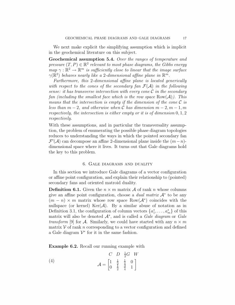
Example 6.2. Recall our running example with

(4)

C D 12G W

A =

[

1 12

14

00 1

234

1

]


[W] [C]

[G]

[D]

G+

CD

D

C+W

GC+W

GD+W

(c)

12W G D C

W* C*

G*

D*

F(A)A*

(a) (b)

A

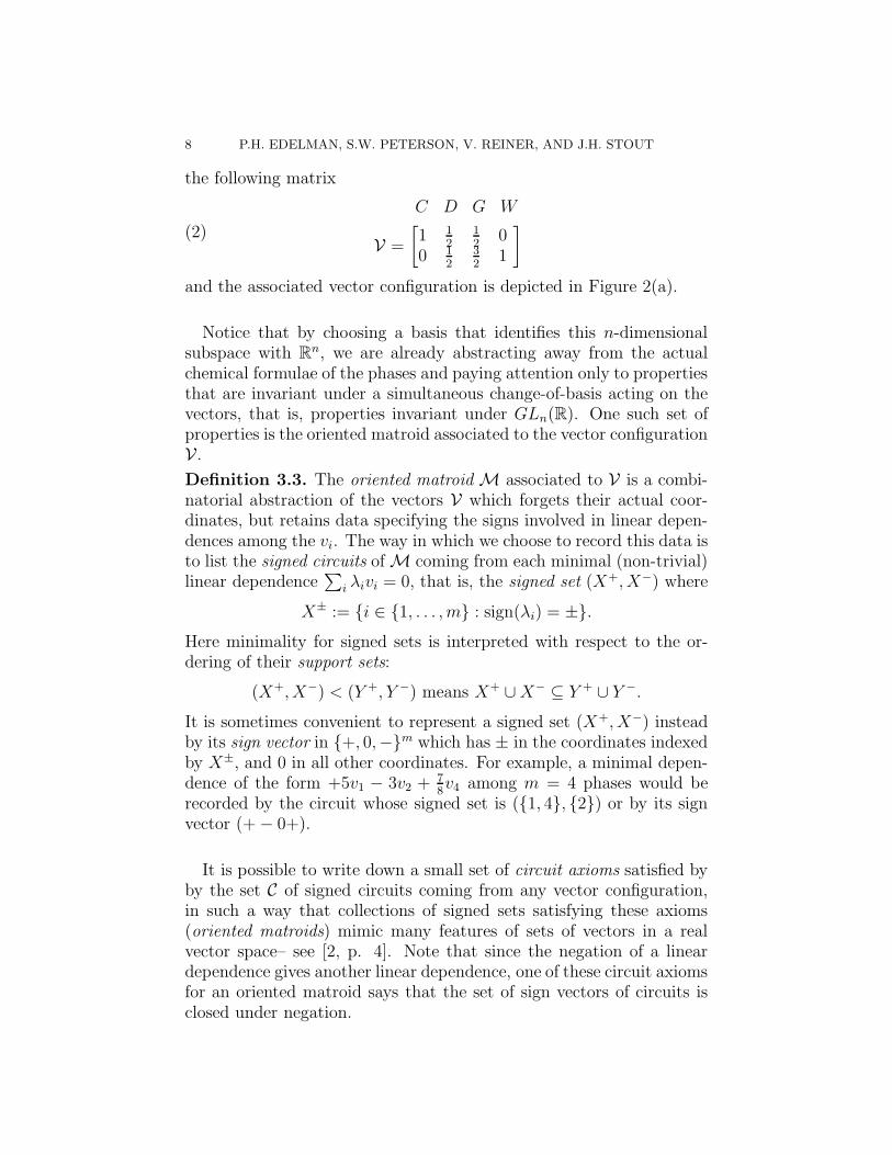
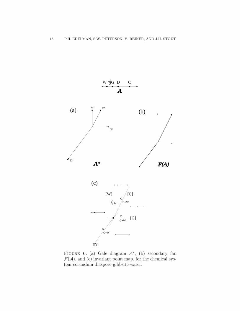
Figure 6. (a) Gale diagram A∗, (b) secondary fanF(A), and (c) invariant point map, for the chemical sys-tem corundum-diaspore-gibbsite-water.


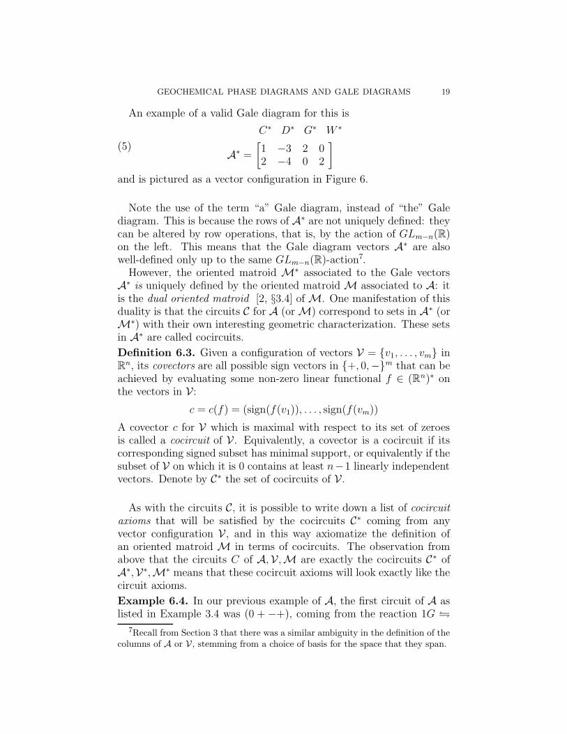
An example of a valid Gale diagram for this is

(5)

C∗ D∗ G∗ W ∗

A∗ =

[

1 −3 2 02 −4 0 2

]

and is pictured as a vector configuration in Figure 6.

Note the use of the term “a” Gale diagram, instead of “the” Galediagram. This is because the rows of A∗ are not uniquely defined: theycan be altered by row operations, that is, by the action of GLm−n(R)on the left. This means that the Gale diagram vectors A∗ are alsowell-defined only up to the same GLm−n(R)-action7.

However, the oriented matroid M∗ associated to the Gale vectorsA∗ is uniquely defined by the oriented matroid M associated to A: itis the dual oriented matroid [2, §3.4] of M. One manifestation of thisduality is that the circuits C for A (or M) correspond to sets in A∗ (orM∗) with their own interesting geometric characterization. These setsin A∗ are called cocircuits.

Definition 6.3. Given a configuration of vectors V = {v1, . . . , vm} inR

n, its covectors are all possible sign vectors in {+, 0,−}m that can beachieved by evaluating some non-zero linear functional f ∈ (Rn)∗ onthe vectors in V:

c = c(f) = (sign(f(v1)), . . . , sign(f(vm))

A covector c for V which is maximal with respect to its set of zeroesis called a cocircuit of V. Equivalently, a covector is a cocircuit if itscorresponding signed subset has minimal support, or equivalently if thesubset of V on which it is 0 contains at least n−1 linearly independentvectors. Denote by C∗ the set of cocircuits of V.

As with the circuits C, it is possible to write down a list of cocircuitaxioms that will be satisfied by the cocircuits C∗ coming from anyvector configuration V, and in this way axiomatize the definition ofan oriented matroid M in terms of cocircuits. The observation fromabove that the circuits C of A,V,M are exactly the cocircuits C∗ ofA∗,V∗,M∗ means that these cocircuit axioms will look exactly like thecircuit axioms.

Example 6.4. In our previous example of A, the first circuit of A aslisted in Example 3.4 was (0 + −+), coming from the reaction 1G �

7Recall from Section 3 that there was a similar ambiguity in the definition of thecolumns of A or V , stemming from a choice of basis for the space that they span.


1D + 1W . In A∗ this is a cocircuit representing the fact that the linespanned by C∗ has G∗ on one side and D∗, W ∗ on the opposite side,i.e., there exists a linear functional f for which

f(C∗) = 0, f(D∗) > 0, f(W ∗) > 0, and f(G∗) < 0.

How does the Gale diagram A∗ relate to the pointed secondary fanF ′(A)? The relationship comes from looking at the positive conesspanned by the vectors of A∗.

Definition 6.5. Given any set W = {w1, . . . , wk} of vectors in RN ,

define the positive cone spanned by W to be

pos(W ) :=

{

k∑

i=1

ciwi ∈ RN : ci > 0 for all i

}

.

If the set of vectors W happen to be linearly independent, then pos(W )is called a (relatively open) simplicial cone.

Recall that the affine point configuration A corresponds to an acyclicvector configuration. It is a consequence of oriented matroid duality[2, Proposition 4.8.9] that A∗ will be totally cyclic, that is, the origin0 lies in the cone pos(A∗). As a consequence, the collection of positivecones spanned by subsets of A∗ will cover the column space Col(A∗),and this covering is closely related to the pointed secondary fan F ′(A):

Theorem 6.6. [3, §4] The column space Col(A∗) has a natural iden-tification with the (m − n)-dimensional subspace complementary toRow(A) within R

m covered by the pointed secondary fan F ′(A).Furthermore, under this identification, the cones of F ′(A) are exactly

the common refinement of all the open simplicial cones pos(W ) spannedby linearly independent subsets W of the Gale (column) vectors A∗.

One can be more precise about this relationship:

Theorem 6.7. [3, Lemma 4.3] Given a coherent triangulation ∆ ofA, the corresponding (m − n)-dimensional cone in the secondary fanF ′(A) is the intersection

⋂

σ∈∆

pos(A∗ − σ∗)

where here σ runs through the vertex sets of the (n − 1)-dimensionalsimplices in the triangulation ∆, and

σ∗ := {a∗i : ai ∈ σ}.


Example 6.8. Because the corundum-diaspore-gibbsite-water exam-ple of A has m = 4 and n = 2, so that m = n + 2, the pointedsecondary fan F ′(A) is 2-dimensional. Therefore its top-dimensionalcones are simply the sectors between cyclically adjacent Gale vectorsin A∗. These cones are depicted in Figure 6(b). In (c) of the samefigure, these regions are labelled (as part of the geochemists’ invari-ant point map; see Section 8 below) by their corresponding coherenttriangulations.

For example, the sector lying between the Gale vectors W ∗ and D∗

corresponds to a triangulation ∆ having two segments {GW, CG}. Thisagrees with Theorem 6.7: the complementary sets {C∗D∗, D∗W ∗} areexactly the ones whose positive cones contain this sector. On the otherhand, the sector between between D∗, G∗ lies in the positive cone of noother pairs of Gale vectors, and hence corresponds to the triangulationhaving only one segment, namely the one with vertices A− {D, G} ={C, W}.

Sections 8 and 9 will closely explore the consequences of the geometryof the Gale diagram for phase diagrams when m is at most n + 3. Butfirst we must further explore more general geometric questions.

7. Geometry of the phase diagram in general

In this section we will explain the relationship between Gibbs’ phaserule (e.g. [21]) and the secondary fan, and how the phase rule predictsthe dimension of various stability fields. We then look closely at themeaning of 2, 1, and 0-dimensional regions in the phase diagram, relat-ing them to m, m − 1, and m − 2-dimensional cones in the secondaryfan.

When one fixes particular molar fractions xi of each of the (rescaled)phases ai in A initially contained in a particular sample, the discussionof Section 5 shows how to predict the stable assemblage of phases whichwill result after allowing the system to find chemical equilibrium. Theinitial molar fractions give a point

∑

i xiai = 1 with∑

i xi = 1 whichlies in the convex hull of A, and lifts to a point

∑

i xiai which lies in

the convex hull of A, but may or may not lie in the lower convex hull.After performing reactions which affect the fractions xi ( but preservethe condition

∑

i xi = 1 due to our re-scaling) to reach chemical equi-

librium, the lifted point∑

i xiai will evenutally lie in a unique face F

of the lower hull of A. The lifted points A′ ⊂ A which happen tolie on this face F lie above a subset A′ ⊂ A of the original phases,that is A′ are those phases which appear with non-zero fraction in this


chemical equilibrium, and A′ labels a polytope F which is part of thecorresponding coherent subdivision of A.

Gibbs’ phase rule relates three quantities relevant to this situation:

• the number of phases m′ = |A′|(≤ m = |A|) participating inthis chemical equilibrium,

• the number of components n′(≤ n) of the subsystem A′, thatis, the dimension of the subspace of chemical composition spacespanned by A′, and

• the number of degrees of freedom f in (T, P ) which one canvary while maintaining these same phases in equilibrium, or inother words, the dimension of the union of all regions in thephase diagram which have A′ labelling one of the polytopes Fin their corresponding subdivision of A.

Proposition 7.1. (Gibbs’ phase rule) With the above notations,

f = n′ + 2 − m′.

In particular, one can have at most n′ + 2 phases that involve n′ com-ponents in chemical equilibrium.

Note that in the geochemical literature, the phase rule is often statedas

f ≤ n + 2 − m′,

which is consistent with the fact that n′ ≤ n.

Example 7.2. In Figure 1, the triple point has an assemblage of m′ = 3phases in equilibria (ice, water, steam), with n′ = 1 and f = 0, whilethe assemblage consisting of pure ice has m′ = n′ = 1 and f = 2.

In Figure 6(c), the line segment DW corresponds to a stable assem-blage {D, W} in two different divariant regions and the curve that sep-arates them (all in the upper right), so f = 2, and it has m′ = n′ = 2.The assemblage {D, G, W} is stable only along the univariant curvelying between the two aforementioned divariant regions so f = 1, andit has m′ = 3, n′ = 2. The quadruple point in the middle (f = 0) ofthe diagram has all 4 phases in equilibrium, that is, m′(= m) = 4, andn′(= n) = 2.

We give here a proof of Gibbs’ phase rule in terms of the secondaryfan F(A) in R

m.

Proof. There is a cone C in the secondary fan consisting of those vectorsg ∈ R

m for which the lifted points A have A′ lying on a face F of thelower hull: this cone is the intersection of the vector space V on whichthe lifted points A′ all lie on a single n′-dimensional affine subspace


with the half-spaces given by various inequalities that assert all theother lifted points ai in A − A′ lift above this affine subspace. Thesubspace V is defined by m′ − n′ linear conditions: after choosing theheight coordinates of g to lift n′ of the elements A′ which are affinelyindependent, the remaining m′ − n′ coordinates of must be lifted toheights which are linear functions of those first n′ heights. Thus V hasdimension m− (m′ − n′). The fact that lifting all the points A−A′ to

any sufficiently large heights will force F to be in the lower hull showsthat the cone C obtained by intersecting V with the various half-spaceinequalities will have the same dimension as V , namely m− (m′ − n′).

By Proposition 5.3 and Assumption 5.4, the union of all regions inthe phase diagram which have A′ labelling one of the polytopes F intheir corresponding subdivision of A comes from the the transverseintersection of an affine 2-plane with the cone C. If m′ − n′ > 2,there would be no intersection due to Assumption 5.4. If m′ − n′ ≤2, then since we assumed that these phases A′ could exist in stableequilibrium, there must be a non-empty intersection. Depending uponwhether m′ − n′ = 0, 1, or 2, this transverse intersection of C withan affine 2-plane will have dimension f = 2, 1, or 0 respectively, i.e.f = 2 − (m′ − n′) = n′ + 2 − m′. �

Understanding the 2, 1, and 0-dimensional regions in the phase di-agram amounts to understanding the cones of dimensions m, m − 1,and m − 2 in the secondary fan F(A) or equivalently, the cones ofdimensions m − n, m − n − 1, m − n − 2 in the pointed secondary fanF ′(A). The 2-dimensional regions in the phase diagram correspondto the top-dimensional cones in F(A) (or F ′(A)), which are labelledby the coherent triangulations of A in the manner described in The-orem 6.7, and there is little to add to that description. The moreinteresting cases are those of the 1 and 0 dimensional stability fields.

7.1. Bistellar operations and 1-dimensional stability fields. The1-dimensional curves separating the regions in the phase diagrams cor-respond to natural transformations on triangulations of A called bistel-lar operations, that are closely related to the circuits of A. We discussthese now somewhat informally; for a more formal treatment, see [10,Chapter 7 §2C].

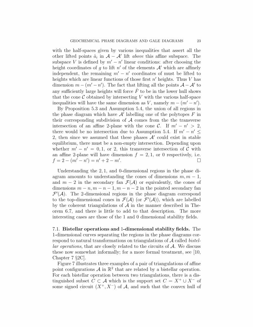
Figure 7 illustrates three examples of a pair of triangulations of affinepoint configurations A in R

2 that are related by a bistellar operation.For each bistellar operation between two triangulations, there is a dis-tinguished subset C ⊂ A which is the support set C = X+ ∪ X− ofsome signed circuit (X+, X−) of A, and such that the convex hull of


Diagonal flip

Inserting/removing a vertex

Figure 7. Three examples of pairs of bistellar opera-tions for triangulations of affine point configurations Ain R

2.

C is triangulated (differently!) in the two triangulations. In this case,we say that the bistellar operation is supported on the circuit C. Notethat in the first two examples in Figure 7 this circuit C has a full 2-dimensional convex hull, but as the third example illustrates, C canhave a convex hull of lower dimension.

Recall that a circuit C = X+ ∪ X− of A corresponds to a cocircuitof A∗, that is there is an (m − n − 1)-dimensional hyperplane HC

spanned by the Gale vectors indexed by A − C which separates theGale vectors indexed by X+ from those indexed by X−. When C isthe circuit supporting a bistellar operation between two triangulations,this reflects the following geometry of pointed secondary fans.

Proposition 7.3. [10, §7.2.C] Two triangulations ∆, ∆′ differ by abistellar operation supported on a signed circuit C if and only if theircorresponding top dimensional cones in F ′(A) are adjacent along a wallwhose linear span is the hyperplane HC .


This has an interpretation for the temperature pressure phase dia-gram which is well-known to geochemists: the segments of curves sepa-rating regions in the phase diagram are always portions of a larger curvecorresponding to some minimal reaction possible among the phases inthe chemical system. Two regions will be adjacent and separated bysuch a curved segment if and only if their corresponding triangulationsdiffer by retriangulating the convex hull of the phases involved in thatreaction.

It is also useful to think of a bistellar operation as represented bythe coherent polytopal subdivision that labels the wall between thetwo top dimensional cones guaranteed by the previous proposition. Inthe language of Gibbs’ phase rule, this subdivision contains a specialpolytopal face F labelled by a subset A′ ⊂ A having m′ = n′ + 1;namely A′ is the support set of the circuit C. Note that if n′ = nthen F is a full (n − 1)-dimensional polytope in the subdivision, andall the other full-dimensional polytopes in the subdivision are (n− 1)-dimensional simplices.

A reasonable question at this point is, “How well do the bistellaroperations tie together the set of all triangulations of A— is it possibleto connect any two triangulations of a point set A by a sequence ofbistellar operations?” The answer has important consequences for cal-culating the set of triangulations of A: the algorithms (e.g. [20]) thatstart with one triangulation and find the rest bistellarly connected toit by performing all possible bistellar operations are much faster thanalgorithms that find all triangulations by the currently available tech-niques [7, 20].

Unfortunately, the answer to the above question is “No” in general:Santos [22, 23] has recently produced examples of triangulations ofaffine point configurations that are connected to no other triangulations(!) by bistellar operations. Fortunately, however there are positiveresults relevant for the geochemical applications:

• All triangulations are connected by bistellar operations whenn ≤ 3 [14],

• the same holds when m − n ≤ 3 [1], and• the subset of coherent triangulations are always connected by

bistellar operations [10].

In particular, this last result allows one to rely on the very fast bis-tellar flip algorithms of [20] (utilized in [18]) to find all of the coherenttriangulations.

7.2. Invariant points and indifferent crossings. We conclude thissection with an informal discussion of 0-dimensional regions in the


phase diagram. These will correspond to cones of dimension m − 2in F(A) or cones of dimension m − n − 2 in F ′(A). These correspondto coherent polytopal subdivisions of A of two possible types, andtherefore give rise to two distinct types of points in the phase diagram:invariant points and indifferent crossings.

Definition 7.4. If a coherent polytopal subdivision of A correspondsto a cone of dimension m − 2 in F(A), then one of the polytopes F ′

in the subdivision might correspond to a stable assemblage A′ havingm′ = n′+2 phases. When this occurs, the same holds for every polytopein the subdivision which contains F ′ as a face. However, the remainingpolytopes which do not contain F ′ will all be simplices.

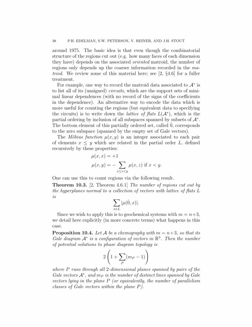
It is in this situation that geochemists reserve the term invariantpoint for the corresponding 0-dimensional region in the phase diagram.In this situation it is possible for all of the phases in A′ to co-existin chemical equilibrium, but one cannot vary (T, P ) at all while main-taining this. For example, the central point in Figures 1 and 6(c) areinvariant points, as are the points labelled [B], [C], [D], [G], [W ] withinthe diagrams labelling regions in Figure 12.

Geochemists usually label the invariant point by the phases B :=A−A′ not involved in the invariant equilibrium. It is also well-knownto geochemists that the local structure of the phase diagram around aninvariant point is similar to the corresponding phase diagram with m′ =n′ + 2 for the chemical subsystem A′. This corresponds to the knownfact [4] that the local structure of the pointed secondary fan F ′(A)about the cone pos(B) and the structure of the fan F ′(A′) = F ′(A −B) coincide, reflecting the fundamental duality between deletion andcontraction in (oriented) matroid theory: the dual point configuration(A−B)∗ to the deletion A−B is isomorphic to the contraction A∗/B∗.

Definition 7.5. On the other hand, when a cone in F(A) has dimen-sion m − 2, there can also be two polytopes F ′ and F ′′ in the corre-sponding polytopal subdivision, neither contained as a face of the other,corresponding to stable assemblages A′ and A′′ with m′ = n′ +1, m′′ =n′′ + 1. The polytopes in the subdivision containing neither of F ′ orF ′′ will all be simplices. For each of A′ or A′′ individually, the union ofregions in the phase diagram where they occur as a stable assemblagecorresponds to a cone of dimension m− 1 in F(A), and a curve in thephase diagram coming from a minimal reaction possible in A. Thesetwo curves intersect at what is called an indifferent crossing, whereeither A′ or A′′ might exist in equilibrium (as might assemblages corre-sponding to other simplices in the subdivision), but the union A′ ∪A′′


12 G D CW

I

12 G D CW

I

12 G D CW

I

(a)

Gibbsenergy

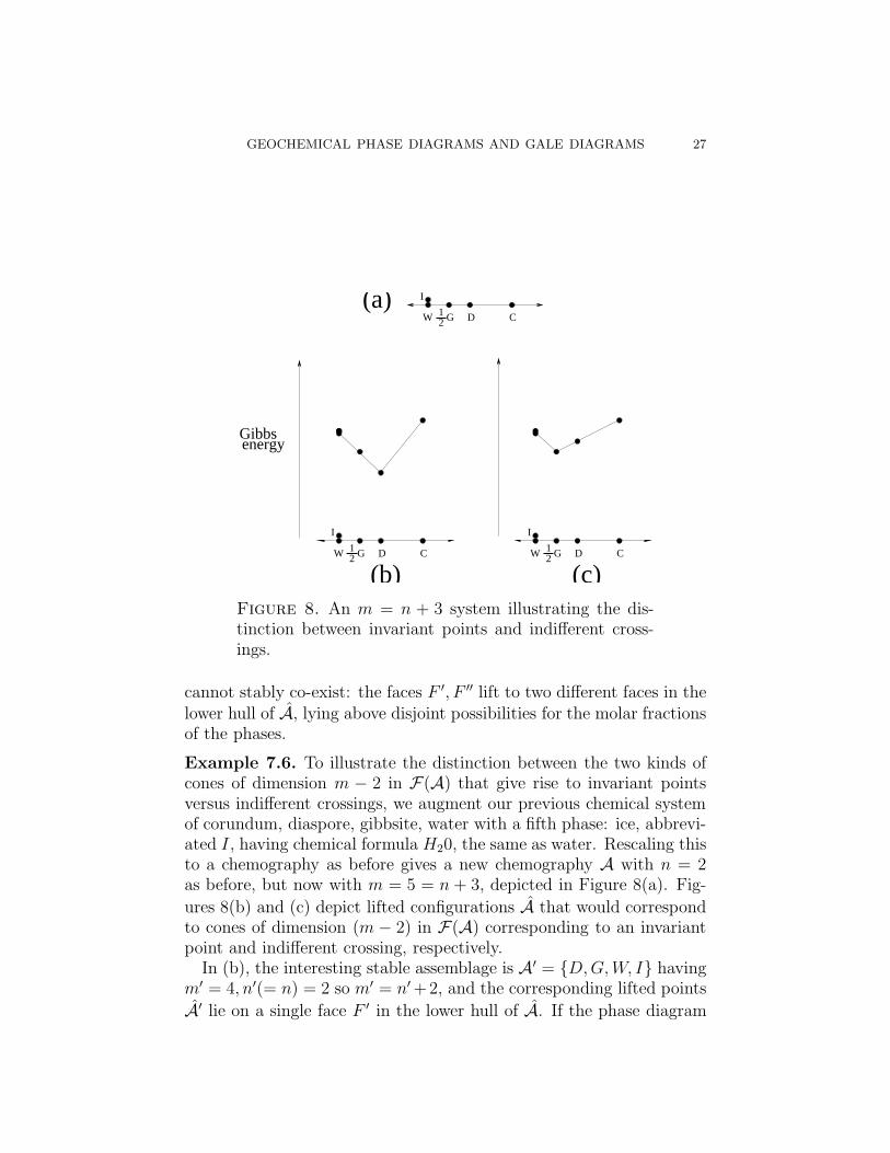
(b) (c)Figure 8. An m = n + 3 system illustrating the dis-tinction between invariant points and indifferent cross-ings.

cannot stably co-exist: the faces F ′, F ′′ lift to two different faces in thelower hull of A, lying above disjoint possibilities for the molar fractionsof the phases.

Example 7.6. To illustrate the distinction between the two kinds ofcones of dimension m − 2 in F(A) that give rise to invariant pointsversus indifferent crossings, we augment our previous chemical systemof corundum, diaspore, gibbsite, water with a fifth phase: ice, abbrevi-ated I, having chemical formula H20, the same as water. Rescaling thisto a chemography as before gives a new chemography A with n = 2as before, but now with m = 5 = n + 3, depicted in Figure 8(a). Fig-

ures 8(b) and (c) depict lifted configurations A that would correspondto cones of dimension (m − 2) in F(A) corresponding to an invariantpoint and indifferent crossing, respectively.

In (b), the interesting stable assemblage is A′ = {D, G, W, I} havingm′ = 4, n′(= n) = 2 so m′ = n′ +2, and the corresponding lifted points

A′ lie on a single face F ′ in the lower hull of A. If the phase diagram


were to contain a point corresponding to this cone of F(A), it wouldbe an invariant point, labelled [C] for the missing phase corundum notin A′.

In (c), there are at least two interesting stable assemblages: A′ ={W, I} with m′ = 2, n′ = 1, and A′′ = {C, D, G} with m′′ = 3, n′ = 2,so that m′ = n′ + 1, m′′ = n′′ + 1, and their corresponding lifted pointsA′, A′′ span different faces F ′, F ′′ of the lower hull of A. If the phasediagram were to contain a point corresponding to this cone of F(A), itwould be an indifferent crossing, lying at the intersection of two curvescorresponding to the two circuits (reactions) involving the phases A′

and A′′.

8. The case m = n + 2: phase diagram = Gale diagram

After dispensing quickly with the cases m = n and m = n + 1, inthis section we examine in detail the structure of Gale diagram A∗, thepointed secondary fan F ′(A), and the phase diagram when m = n+2.The conclusion is that they all look roughly the same in this case.

When m = n, the m phases cannot perform any reactions that pre-serve mass-balance, and so are mutually inert and nothing can happen.

When m = n + 1, not much interesting happens. There is ex-actly one reaction possible, corresponding to the unique signed circuitC = (X+, X−) of A. The Gale diagram A∗ is a set of vectors lying onthe real line R

1 with their tails at the origin 0. Those a∗i having i ∈ X+

will point in the positive direction, those with i ∈ X− will point in thenegative direction, and those i ∈ {1, . . . , m} − (X+ ∪ X−) will be zerovectors pointing nowhere. The secondary fan F ′(A) decomposes the R

1

into two cones: the two rays emanating from the origin in the positiveand negative directions. These rays correspond to the two triangula-tions of A which differ by a bistellar operation supported on C. At aparticular temperature and pressure, the Gibbs energy of the ensembleof products/reactants, whichever is lower, will force the reaction to runin one direction or another, so that the stable assemblages will corre-spond to the simplices of one or the other triangulation. In this case,the phase diagram consists of two divariant regions separated by theunivariant curve corresponding to the single reaction.

When m = n + 2, things start to become interesting. First, we canassume without loss of generality that there are no indifferent phases8,that is, every phase participates in some possible reaction or phase

8An indifferent phase would give rise to an element ai of the oriented matroidfor A known as an isthmus or coloop, and also to a zero Gale vector a∗

i = 0.


change. By excluding indifferent phases, we know that the Gale dia-gram A∗ has m non-zero Gale vectors a∗

1, . . . , a∗m, although it is possible

that some differ by positive scalar multiples and hence point in the samedirection9. The pointed secondary fan F ′(A) will look very similar tothe Gale diagram, having at most m rays emanating from the origin,pointing in the directions of the Gale vectors, and 2-dimensional coneslying between cyclically adjacent Gale vectors. According to Proposi-tion 5.3, the phase diagram should look roughly like a 2-dimensionalslice of this 2-dimensional pointed secondary fan F ′(A), that is, likeF ′(A) itself. Hence the phase diagram will closely resemble the Galediagram A∗.

Roughly speaking, geochemists have known some version of this,in the guise of a method for constructing their invariant point mapsas schematic representations of the local picture around an invariantpoint, based on knowledge of the minimal reactions possible among thephases. Their method uses Schreinemakers’ fundamental axiom [25,30], which is a re-formulation of the oriented matroid duality assertionthat the circuits of A coincide with the cocircuits of A∗. The axiomsassert that

• each phase ai should label some univariant reaction half-lineemanating from the invariant point, corresponding to a minimalreaction among the remaining phases other than ai, and

• the extension of this half-line to a line through the origin shouldseparate the other univariant reaction half-lines into those cor-responding to the two sides of the reaction in question.

In other words, each Gale vector a∗i lies on a line through the origin

corresponding to a cocircuit of A∗, which corresponds to a circuit ofA.

Using this rule, one can sketch the invariant point map by proceedingthrough the list of minimal reactions among the phases, and using theaxiom to place the half-lines around each other in cyclic order. Thereis an initial choice of orientation one must make for the diagram usingthe first reaction (should the reactant/products/missing-phase-half-linego in clockwise or counterclockwise order around the invariant point?),but after that the picture is determined. To decide which orientation isconsistent with the actual geochemical phase diagram (i.e. to determinethe actual placement of the image surface γ(R2) within the secondaryfan F(A)), some thermodynamic data is required.

9This will happen whenever there are affine hyperplanes in Rn−1 that contain

all but two of the points of A


Example 8.1. Figure 6(c) shows the invariant point map constructedfor the corundum-diaspore-gibbsite-water example. Note that we haveused the geochemical conventions of labelling the univariant reactionhalf-lines emanating from the invariant point by the phase(s) missingfrom the reaction, putting the product/reactants on either side of theline, and indicating with dashes the metastable extensions of these half-lines.

9. The case m = n + 3: phase diagram = affine Galediagram

We next examine in detail the structure of the Gale diagram A∗, thepointed secondary fan F ′(A), and the phase diagram when m = n+3.The conclusion is that two methods used by geochemists to reducean essentially 3-dimensional picture to two dimensions have parallelconstructions in discrete geometry, and the phase diagram bears a closeresemblance to a 2-dimensional affine Gale diagram.

When m = n + 3, we can again assume without loss of generalitythat there are no indifferent phases, and hence no zero Gale vectorsa∗

i . However we make no other genericity assumptions for the moment.The Gale diagram A∗ is a vector configuration in R

3. As before, someGale vectors may differ by a positive scalar multiple and hence giverise to the same ray in the secondary fan F ′(A), so we know therewill be at most m such rays. Note that unlike the case m = n + 2,here the cones of the pointed secondary fan F ′(A) can be more exoticin shape: they are intersections of the 3-dimensional simplicial conesspanned by linearly independent subsets of A∗, and hence can havearbitrary polygonal cross-sections.

The one-dimensional cones (rays) in F ′(A) will correspond to 0-dimensional (point) regions in the phase diagram when they intersectthe image surface γ(R2) of the Gibbs energy map. As discussed in Sub-section 7.2, these points will either be indifferent crossings or invariantpoints. Since the invariant points correspond to chemical subsystemsA′ ⊂ A which have m′ = n′ + 2, if we have n′ = n (as happens generi-cally) then |A′| = |A|− 1, that is, there is exactly one phase ai missingfrom A′, and the corresponding ray in F ′(A) is spanned by the Galevector a∗

i . This is the reason that invariant points in phase diagramswith m = n + 3 are generically labelled by the single phase missingfrom the invariant equilibrium at that point. As also discussed in Sub-section 7.2, the local structure about the invariant point will look likethe invariant point map for the m′ = n′ + 2 subsystem A′.


p i pj

pj p i

− −

− −

stable reaction line

metastable reaction linemetastable reaction line

reaction linedoubly−metastable

i j

j i

* *

**

a a

a a

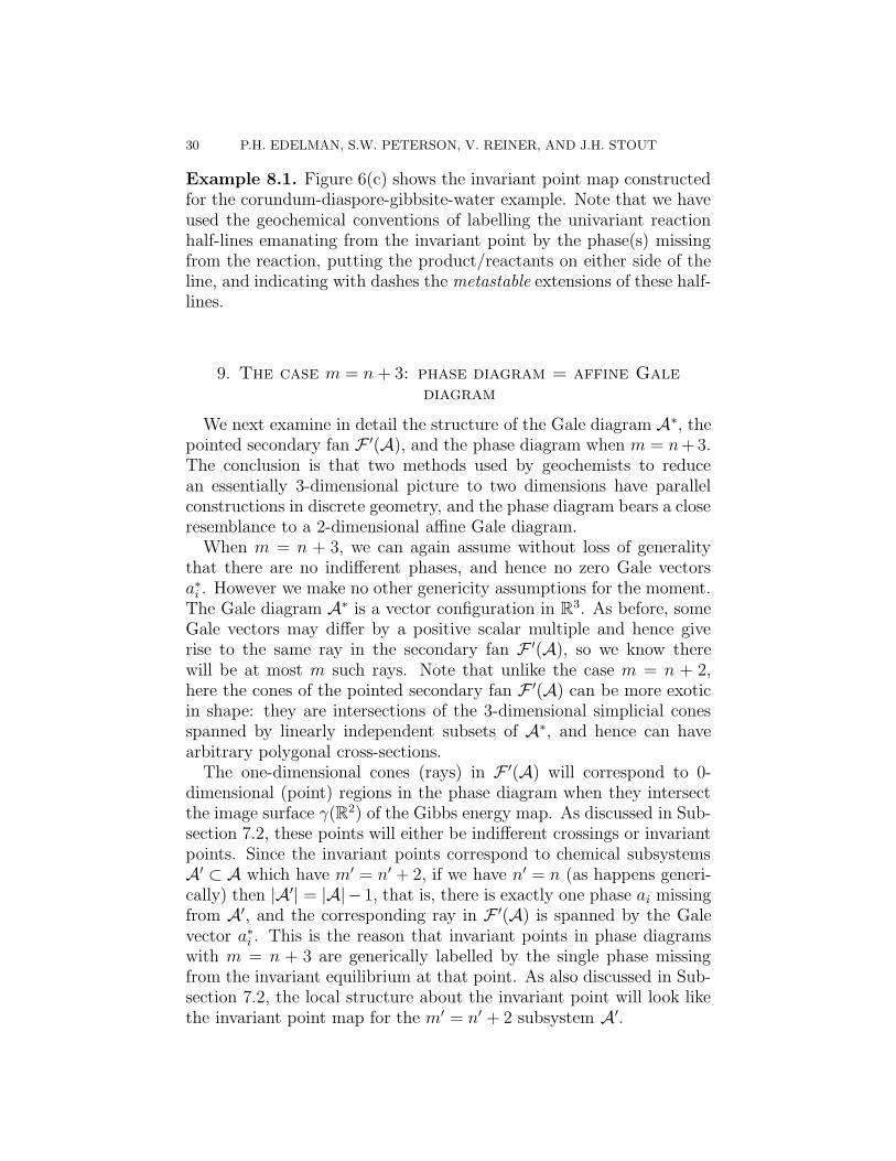
Figure 9. A typical reaction loop defined by two Galevectors a∗

i and a∗j .

Vector configurations in R3 (like A∗) can be difficult to visualize. We

discuss two methods that have been commonly used to cut down thedimension by one (and produce a picture closer in spirit to the phasediagram): the spherical representation and affine Gale diagrams.

9.1. The spherical representation: closed nets. Intersecting thepointed secondary fan F ′(A) in R

3 with a unit sphere centered aboutthe origin gives a useful spherical representation, similar to what hasbeen called a closed net in [29]. In the conventions for the closed net,

one includes not only the point of intersection with the sphere pi :=a∗

i

|a∗

i|

for each ray spanned by a Gale vector a∗i (represented by a black dot

labelled by the corresponding phase ai), but also its negation −pi (rep-resented by a white dot labelled similarly)10. Furthermore, the arcrepresenting the intersection curve on the sphere of a 2-dimensionalcone in F ′(A) is augmented to be part of a great circle called a reac-tion loop, corresponding to the unique minimal reaction (circuit of A,cocircuit of A∗) to which it is associated. Typically such a reaction willinvolve all but two phases ai, aj (although this will not always be thecase when A is not generic and therefore has some circuits of smaller

10This supplementation of the Gale diagram A∗ by adding in negations of allits vectors is reminiscent of the Lawrence construction [2, §9.3] in oriented matroidtheory.


pj− p i−

p ipj

pj− p i−

pj− p i−

p i pj

pjp i

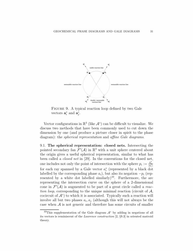
Figure 10. The four possible projections of a reactionloop onto an affine 2-plane.

[G] [C] [W]

[B]

[D]

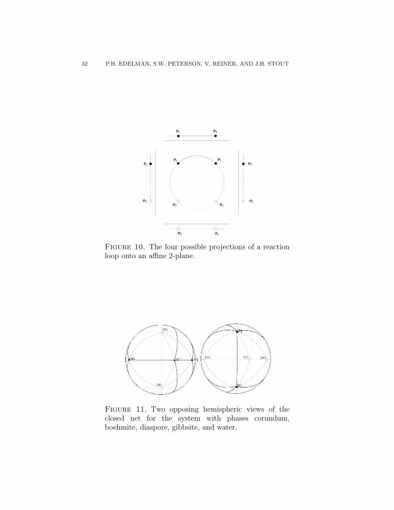
Figure 11. Two opposing hemispheric views of theclosed net for the system with phases corundum,boehmite, diaspore, gibbsite, and water.


support). As one traverses such a typical reaction loop, one passesthrough four arcs as depicted in Figure 9.

The point of the closed net representation is that a hemispherical orplanar projection of it from some angle should give a schematic pictureof the actual phase diagram. Which projection occurs in nature willdepend upon the location and orientation of the image surface γ(R2) ofthe Gibbs energy map from Section 5 inside the secondary fan F(A).Under our Assumption 5.4, one of each pair {pi,−pi} will appear in theprojection, and there are four possibilities for the portion of a typicalreaction loops that will appear in the projection, depicted in Figure 10.

Example 9.1. We add a fifth phase (different from the ice added inExample 7.6) to our original example of corundum, diaspore, gibbsite,and water: the mineral boehmite (B) which is a polymorph of dias-pore, that is, it has the same chemical formula AlO(OH), but differentcrystal structure. Thus B, D become parallel elements in the orientedmatroid M for this new point configuration A, having m = 5 andn = 2, so that m = n + 3.

We have

(6)

C D B 12G W

A =

[

1 12

12

14

00 1

212

34

1

]

and a valid Gale transform is

(7)

C∗ D∗ B∗ G∗ W ∗

A∗ =

1 0 0 −4 30 1 0 −2 10 0 1 −2 1

Two opposite hemispheric views of the closed net for this exampleare depicted in Figure 11. Note that the parallel elements B, D in Agive rise to a circuit

C D B G W0 + − 0 0

that corresponds to a cocircuit of A∗: the Gale vectors C∗, G∗, W ∗ arecoplanar, and their corresponding points on the closed net lie on a greatcircle which separates D∗ from B∗.

9.2. Two-dimensional affine Gale diagrams. The affine Gale di-agram is simply an affine point configuration in R

2 used to encodethe 3-dimensional vector configuration A∗; see [33, Definition 6.17], [2,


§9.1]. Arbitrarily choose a 2-dimensional affine plane Γ in R3 to “slice”

the Gale vectors: if this plane Γ is defined by the equation f(x) = cfor some generic linear functional f ∈ (R3)∗ and some positive value c,

then we replace each Gale vector a∗i by the unique point c

a∗

i

f(a∗

i)

in its

span that lies in this plane Γ. Color these rescaled Gale points in Γblack or white depending upon whether f(a∗

i ) > 0 or f(a∗i ) < 0. Since

A was an affine point configuration and hence A∗ is a totally cyclicvector configuration, there will always be both black and white pointsin the affine Gale diagram, regardless of how the functional f is chosen.

We can further annotate the affine Gale diagram by drawing in linesegments that correspond to the intersections of 2-dimensional conesfrom F ′(A) with the plane Γ that happen to connect the black pointsin the diagram. Bearing in mind Assumption 5.4, the choice of thefunctional f (equivalently, the choice of the plane Γ) corresponds tothe choice of the location of the image surface γ(R2) of the Gibbsenergy map. It follows from Proposition 5.3 that this “decorated affineGale diagram” is a schematic picture for one possible toplogy of thephase diagram. Such schematic pictures, when annotated further withmore arcs of reaction loops using conventions similar to the closed netsdiscussed in Subsection 9.1 above, have appeared in [17] and are calledpotential solutions for the phase diagram topology.

When are two such affine Gale diagrams/potential solutions consid-ered “equivalent”? Fortunately, discrete geometers and geochemistsagree on this: when the assignment of either a black and white dot toeach phase is the same. Equivalently, this means they have the samesign vector (sign(f(a∗

1)), . . . , sign(f(a∗m)) ∈ {+,−}m, or in oriented ma-

troid terminology, that f achieves the same acyclic (re-)orientation (ortope) of the vector configuration A∗ [2, Section 3.8]. This turns out tohave the following geometric re-intepretation: if we regard the func-tional f(x) = f1x1 + f2x2 + f3x3 as its vector of coefficients (f1, f2, f3),then the acyclic orientation achieved by f is determined by which sideof each of the hyperplanes (a∗

i )⊥ normal to the Gale vectors it lies on.

Therefore intersecting this arrangement of hyperplanes (a∗i )

⊥ with theunit sphere in R

3 gives an arrangement of great circles on the sphere(called the Euler sphere in [16]), whose 2-dimensional regions param-etrize the different acyclic orientations/affine Gale diagrams/potentialsolutions.

The method developed in [16] of constructing potential solutionsfor systems with m = n + 3 systems involved looking at each phase,using the method of Schreinemaker from Section 8 to infer the localstructure/invariant point map about the invariant point where that


phase is missing from the assemblage, and then “fitting together” thesevarious invariant point maps to produce the straight line net.

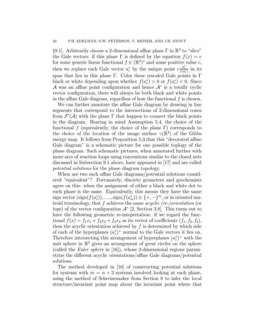
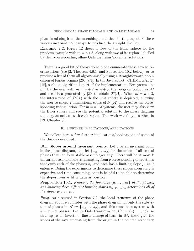
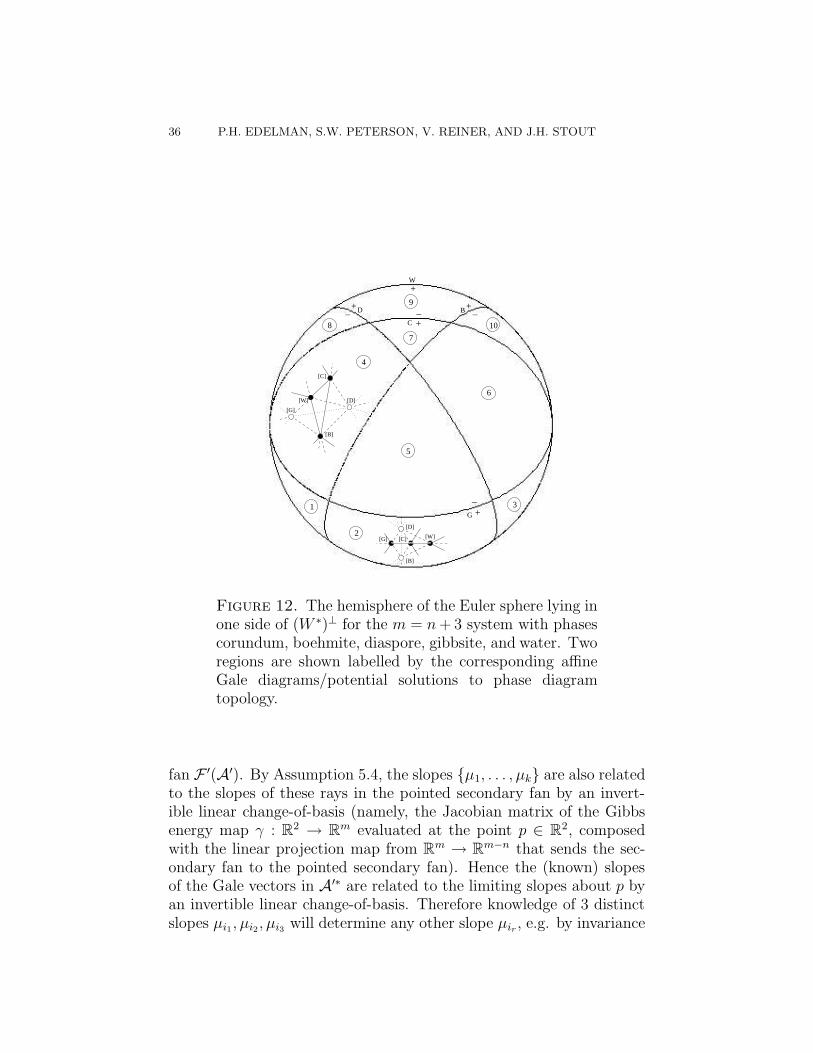
Example 9.2. Figure 12 shows a view of the Euler sphere for theprevious example with m = n+3, along with two of its regions labelledby their corresponding affine Gale diagrams/potential solutions.

There is a good bit of theory to help one enumerate these acyclic re-orientations (see [2, Theorem 4.6.1] and Subsection 10.2 below), or toproduce a list of them all algorithmically using a straightforward appli-cation of Farkas’ lemma [26, §7.3]. In the Java applet “CHEMOGALE”[18], such an algorithm is part of the implementation. For systems in-put by the user with m = n + 2 or n + 3, the program computes A∗

and uses data generated by [20] to obtain F ′(A). When m = n + 3,the intersection of F ′(A) with the unit sphere is depicted, allowingthe user to select 2-dimensional cones of F ′(A) and receive the corre-sponding triangulation. For m = n+3 systems, the user may also viewthe Euler sphere and see the potential solution to the phase diagramtopology associated with each region. This work was fully described in[19, Chapter 3].

10. Further implications/applications

We collect here a few further implications/applications of some ofthe theory developed.

10.1. Slopes around invariant points. Let p be an invariant pointin the phase diagram, and let {a1, . . . , ak} be the union of all sets ofphases that can form stable assemblages at p. There will be at most kunivariant reaction curves emanating from p corresponding to reactionsthat omit each of the phases ai, and each has a limiting slope µi as itenters p. Doing the experiments to determine these slopes accurately isexpensive and time-consuming, so it is helpful to be able to determinethe slopes from as little data as possible.

Proposition 10.1. Knowing the formulae {a1, . . . , ak} of the phases,and knowing three different limiting slopes µi1 , µi2, µi3 determines all ofthe slopes µ1, . . . , µk.

Proof. As discussed in Section 7.2, the local structure of the phasediagram about p coincides with the phase diagram for only the subsys-tem of phases in A′ := {a1, . . . , ak}, and this must be a system withk = n + 2 phases. Let its Gale transform be A′∗ := {a∗

1, . . . , a∗k}, so

that up to an invertible linear change-of-basis in R2, these give the

slopes of the rays emanating from the origin in the pointed secondary


B

C

W

G

D

8

9

10

4

7

6

5

1

2

3

+_ +_+_

+

+

_

[G] [W][C]

[B]

[D]

[W]

[G]

[C]

[D]

[B]

Figure 12. The hemisphere of the Euler sphere lying inone side of (W ∗)⊥ for the m = n + 3 system with phasescorundum, boehmite, diaspore, gibbsite, and water. Tworegions are shown labelled by the corresponding affineGale diagrams/potential solutions to phase diagramtopology.

fan F ′(A′). By Assumption 5.4, the slopes {µ1, . . . , µk} are also relatedto the slopes of these rays in the pointed secondary fan by an invert-ible linear change-of-basis (namely, the Jacobian matrix of the Gibbsenergy map γ : R

2 → Rm evaluated at the point p ∈ R

2, composedwith the linear projection map from R

m → Rm−n that sends the sec-

ondary fan to the pointed secondary fan). Hence the (known) slopesof the Gale vectors in A′∗ are related to the limiting slopes about p byan invertible linear change-of-basis. Therefore knowledge of 3 distinctslopes µi1, µi2, µi3 will determine any other slope µir , e.g. by invariance


under invertible linear transformations of the cross-ratio

(µi1 , µi2 | µi3, µir) :=(µir − µi1)(µi3 − µi2)

(µir − µi2)(µi3 − µi1).

�

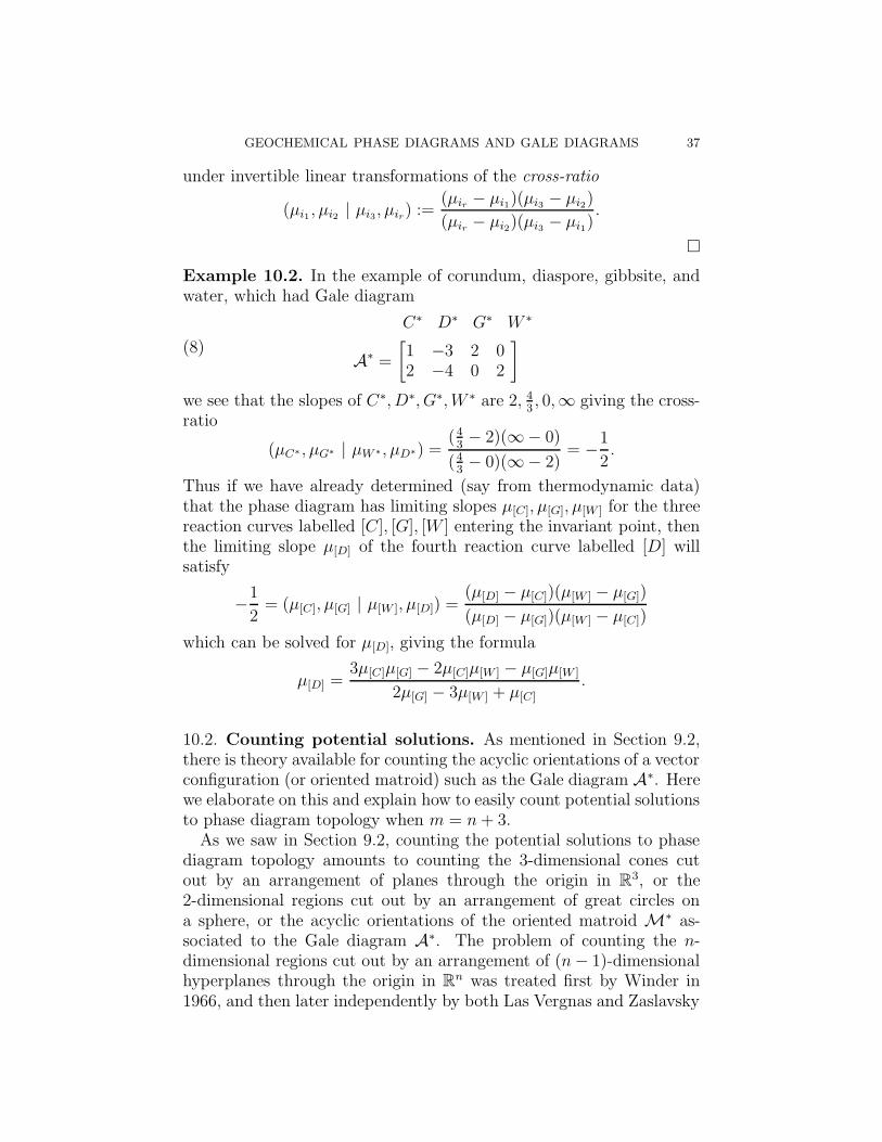
Example 10.2. In the example of corundum, diaspore, gibbsite, andwater, which had Gale diagram

(8)

C∗ D∗ G∗ W ∗

A∗ =

[

1 −3 2 02 −4 0 2

]

we see that the slopes of C∗, D∗, G∗, W ∗ are 2, 43, 0,∞ giving the cross-

ratio

(µC∗, µG∗ | µW ∗, µD∗) =(4

3− 2)(∞− 0)

(43− 0)(∞− 2)

= −1

2.

Thus if we have already determined (say from thermodynamic data)that the phase diagram has limiting slopes µ[C], µ[G], µ[W ] for the threereaction curves labelled [C], [G], [W ] entering the invariant point, thenthe limiting slope µ[D] of the fourth reaction curve labelled [D] willsatisfy

−1

2= (µ[C], µ[G] | µ[W ], µ[D]) =

(µ[D] − µ[C])(µ[W ] − µ[G])

(µ[D] − µ[G])(µ[W ] − µ[C])

which can be solved for µ[D], giving the formula

µ[D] =3µ[C]µ[G] − 2µ[C]µ[W ] − µ[G]µ[W ]

2µ[G] − 3µ[W ] + µ[C]

.

10.2. Counting potential solutions. As mentioned in Section 9.2,there is theory available for counting the acyclic orientations of a vectorconfiguration (or oriented matroid) such as the Gale diagram A∗. Herewe elaborate on this and explain how to easily count potential solutionsto phase diagram topology when m = n + 3.

As we saw in Section 9.2, counting the potential solutions to phasediagram topology amounts to counting the 3-dimensional cones cutout by an arrangement of planes through the origin in R

3, or the2-dimensional regions cut out by an arrangement of great circles ona sphere, or the acyclic orientations of the oriented matroid M∗ as-sociated to the Gale diagram A∗. The problem of counting the n-dimensional regions cut out by an arrangement of (n − 1)-dimensionalhyperplanes through the origin in R

n was treated first by Winder in1966, and then later independently by both Las Vergnas and Zaslavsky


around 1975. The basic idea is that even though the combinatorialstructure of the regions cut out (e.g. how many faces of each dimensionthey have) depends on the associated oriented matroid, the number ofregions only depends up the coarser information recorded in the ma-troid. We review some of this material here; see [2, §4.6] for a fullertreatment.

For example, one way to record the matroid data associated to A∗ isto list all of its (unsigned) circuits, which are the support sets of mini-mal linear dependences (with no record of the signs of the coefficientsin the dependence). An alternative way to encode the data which ismore useful for counting the regions (but equivalent data to specifyingthe circuits) is to write down the lattice of flats L(A∗), which is thepartial ordering by inclusion of all subspaces spanned by subsets of A∗.The bottom element of this partially ordered set, called 0, correspondsto the zero subspace (spanned by the empty set of Gale vectors).

The Mobius function µ(x, y) is an integer associated to each pairof elements x ≤ y which are related in the partial order L, definedrecursively by these properties:

µ(x, x) = +1

µ(x, y) = −∑

x≤z<y

µ(x, z) if x < y.

One can use this to count regions via the following result.

Theorem 10.3. [2, Theorem 4.6.1] The number of regions cut out bythe hyperplanes normal to a collection of vectors with lattice of flats Lis

∑

x∈L

|µ(0, x)|.

Since we wish to apply this is to geochemical systems with m = n+3,we detail here explicitly (in more concrete terms) what happens in thiscase.

Proposition 10.4. Let A be a chemography with m = n+3, so that itsGale diagram A∗ is a configuration of vectors in R

3. Then the numberof potential solutions to phase diagram topology is

2

(

1 +∑

P

(mP − 1)

)

where P runs through all 2-dimensional planes spanned by pairs of theGale vectors A∗, and mP is the number of distinct lines spanned by Galevectors lying in the plane P (or equivalently, the number of parallelismclasses of Gale vectors within the plane P ).


In particular, if A is in general position (in the sense that everysubset of n elements in A are affinely independent, or equivalently,every minimal reaction among the phases involves at least n+1 phases),the number of potential solutions is (cf. [17])

2

(

1 +

(

n

2

))

.

Proof. Since A∗ lives in R3, there are four kinds of elements x in the

lattice of flats:

• x = 0, having µ(0, 0) = +1,• x = `, a line spanned by a Gale vector a∗

i , having µ(0, `) = −1,• x = P , a 2-dimensional plane spanned by Gale vectors, having

µ(0, P ) = −

(

µ(0, 0) +∑

`⊂P

µ(0, `)

)

= mP − 1, and

• x = R3, having

µ(0, R3) = −

(

µ(0, 0) +∑

`

µ(0, `) +∑

P

µ(0, P )

)

= −1 + #{ lines ` spanned by Gale vectors}

+∑

P

(mP − 1)

Adding the absolute values of all of these gives the result stated in theProposition.

In the generic case, since A has n points, there will be n distinctGale vectors A∗, no two of which span the same line `, and there willbe(

n

2

)

different planes P spanned by them (A is generic if and onlyif A∗ is generic by matroid duality). Also, each of these planes willcontain exactly two lines ` so mP −1 = 1. The second assertion followsfrom plugging these values into the first equation. �

Example 10.5. In Figure 12, the Euler sphere shown has 20 regionstotal (10 visible on the hemisphere shown, 10 more on the “underside”).One can compare this with the formula predicted in the proposition,which can be evaluated with the aid of the closed net picture of Galevectors in Figure 11. This figure shows (the intersection with the sphereof ) 8 planes P spanned by pairs of Gale vectors, namely

BC, BG, BW, DG, DC, DW, BD, BGW,


of which the first 7 have mP = 2 and the last has mP = 3. Thus theproposition would predict

2(1 + 7 · (2 − 1) + 1 · (3 − 1)) = 20

regions, as expected.

References

[1] M. Azaola and F. Santos, The graph of triangulations of a point configu-ration with d + 4 vertices is 3-connected. Discrete Comput. Geom. 23 (2000),489–536.

[2] A. Bjorner, M. Las Vergnas, B. Sturmfels, N. White, and G.Ziegler, Oriented Matroids. Cambridge. Cambridge University Press, 1993.

[3] L.J. Billera, P. Filliman, and B. Sturmfels, Constructions and com-plexity of secondary polytopes. Adv. Math. 83 (1990), 155–179.

[4] L.J. Billera, I. M. Gelfand, and B. Sturmfels, Duality and minors ofsecondary polyhedra. J. Combin. Theory Ser. B 57 (1993), 258–268.

[5] R.G. Bland, and M. Las Vergnas, Orientability of matroids, J. Combi-

natorial Theory B 24 (1978), 94–123.[6] H. W. Day, Geometric analysis of phase equilibria in ternary systems of six

phases. Amer. J. Sci. 272 (1972), 711–734.[7] J.A. de Loera, S. Hosten, F. Santos, B. Sturmfels, The polytope of all

triangulations of a point configuration. Doc. Math. 1 (1996), No. 04, 103–119.[8] J. Folkman and J. Lawrence, Oriented matroids. J. Combinatorial Theory

B 25 (1978), 199–236.[9] D. Gale, Neighboring vertices on a convex polyhedron, in “Linear inequalities

and related systems” (H.W. Kuhn and A.W. Tucker, eds.), Annals of Math.

Studies 38, Princeton Univ. Press, Princeton, 1956, pp. 255–263.[10] I.M. Gelfand, M.M. Kapranov, A.V. Zelevinsky, Discriminants, resul-

tants, and multidimensional determinants, Birkhauser, Boston, MA, 1994.[11] B. Grunbaum, Convex Polytopes, New York, Wiley Interscience, 1967.[12] B. Guy and J. M. Pla, Structure of phase diagrams for n-component

(n+k)-phase chemical systems: the concept of affigraphy, Comptes Rendus

de l’Academie des Sciences 324 IIa (1997), 1–7.[13] T.J.B. Holland and R. Powell, R. An enlarged and updated internally

consistent thermodynamic data set with uncertainties and correlations in thesystem K2O−Na20−CaO−MgO−MnO−FeO−Fe2O3 −Al2O3 −T iO2−SiO2 − C − H2 − O2 Journal of Metamorphic Geology 8 (1990), 89–124.

[14] C. L. Lawson, Transforming triangulations, Discrete Math. 3 (1972), 365–372.

[15] C.W. Lee, Regular triangulations of convex polytopes. Applied geometry and

discrete mathematics, 443–456, DIMACS Ser. Discrete Math. Theoret. Com-

put. Sci. 4, Amer. Math. Soc., Providence, RI, 1991.[16] G. Kletetschka and J.H. Stout, Stability analysis of invariant points

using Euler spheres, with an application to FMAS granulites. J. metamorphic

Geol. 17 (1999), 1–14.[17] R.E. Mohr and J.H. Stout, Multisystem nets for systems of n + 3 phases,

American Journal of Science 280 (1980), 143–172.


[18] S.W. Peterson, CHEMOGALE: A Java applet for computing geochemicalphase diagrams, 2000.(Available at www.math.umn.edu/~reiner/CHEMOGALE.html)

[19] S.W. Peterson, Oriented matroid analysis of thermochemical reaction sys-

tems. Masters Thesis (2000), University of Minnesota, Minneapolis.[20] J. Rambau, TOPCOM: Triangulations of Point Configurations and Oriented

Matroids, version 0.2.0.(Available at www.zib.de/rambau/TOPCOM.html.)

[21] J.E. Ricci, The phase rule and heterogeneous equilibrium, D. Van NostrandCompany, Inc., 1951.

[22] F. Santos, A point set whose space of triangulations is disconnected. J. Amer.

Math. Soc. 13 (2000), 611–637.[23] F. Santos, Non-connected toric Hilbert schemes, available at http://arXiv.

org/abs/math.CO/0204044.[24] F. Santos, Triangulations of oriented matroids. Mem. Amer. Math. Soc. 156

(2002), no. 741.[25] F.A.H. Schreinemakers, In-, mono-, and di-variant equilibria, Koninklijke

Academia van Wetenschappen te Amsterdam 18-28(1915-1925), 322 p.[26] A. Schrijver, Theory of Linear and Integer Programming, 1998, Wiley-

Interscience, New York.[27] V. S. Sheplev, Construction of chemographic diagrams. Petrology 4 1 (1996),

97–102.[28] S.I. Usdansky, Some topological and combinatorial properties of c component

(c + 4) phase multisystem nets. Mathematical Geology 19 8 (1987), 793–805.[29] E. Zen, Some topological relationships in multisystems of n + 3 phases I.

General theory; unary and binary systems. American Journal of Science 264

(1966), 401-427.[30] E. Zen Construction of pressure-temperature diagrams for multicomponent

systems as the method of Schreinemakers- A geometric approach, U.S. Geo-

logical Survey Bulletin 1225 (1966), 66 pp.[31] E. Zen Some topological relationships in multisystems of n + 3 phases II.

Unary and binary metastable sequences. American Journal of Science 265

(1967), 871-897.[32] E. Zen and E.H. Rosenboom Jr., Some topological relationships in mul-

tisystems of n + 3 phases III. Ternary systems. American Journal of Science

272 (1972), 677-710.[33] G.M. Ziegler,Lectures on Polytopes, New York, Springer-Verlag, 1995.


Dept. of Mathematics, Vanderbilt University, Nashville, TN 37240-0001

E-mail address : [email protected]

School of Mathematics, University of Minnesota, Minneapolis MN55455


School of Mathematics, University of Minnesota, Minneapolis, MN55455


Department of Geology and Geophysics, University of Minnesota,Minneapolis MN 55455


geochemical phase diagrams and gale diagramsreiner/papers/geology.pdfa geochemistry-discrete...

Documents