geodesic active regions for texture segmentation€¦ · · 2015-07-29geodesic active regions for...

ISS

N 0

249-

6399

appor t de r echerche

THÈME 3

INSTITUT NATIONAL DE RECHERCHE EN INFORMATIQUE ET EN AUTOMATIQUE

Geodesic Active Regions for Texture Segmentation

Nikos PARAGIOS and Rachid DERICHE

N° 3440

Juin 1998

Unité de recherche INRIA Sophia Antipolis2004, route des Lucioles, B.P. 93, 06902 Sophia Antipolis Cedex (France)

Téléphone : 04 92 38 77 77 - International : +33 4 92 38 77 77 — Fax : 04 92 38 77 65 - International : +33 4 92 38 77 65

Geodesic Active Regions for Texture Segmentation

Nikos PARAGIOS and Rachid DERICHE

Thème 3 � Interaction homme-machine,

images, données, connaissances

Projet Robotvis

Rapport de recherche n° 3440 � Juin 1998 � 38 pages

Abstract: This paper proposes a framework for segmenting di�erent textured areas over

synthetic or real textured frames by curves propagation. We assume that the system has the

ability to be taught over di�erent texture prototypes. For each prototype a global statistical

model is generated, as a set of probability density functions attributes from a multi-valued

frame analysis, where di�erent �lter responses are used to create this multi-valued frame.

Then, each prototype is represented by a reliable statistical model. Given an input frame

composed of di�erent texture types, the same bank of �lters is applied. Over the generated

multi-valued frame, we de�ne an energy as a special form of a geodesic active contour

model, a Geodesic Active Region Model, where we integrate boundary �nding and

region based segmentation approaches. This energy is minimized using a steepest gradient

descend method, where smoothing, edge-based, and region statistics forces, move the curve

toward the minimum of the designed objective function. Using the level set formulation

scheme, complex curves can be detected, while topological changes for the evolving curves

are naturally managed. In order to deal with the problem of noise in�uence, as well as to

reduce the required computational cost, a multi-grid approach has also been considered.

Finally, two di�erent methods are used for the level set implementation, the Narrow Band

and the Hermes Algorithm. Very promising experimental results are provided using synthetic

and real textured frames.

Key-words: Texture Segmentation, Filters Bank, Statistical Modeling, Geodesic Active

Contours, Geodesic Active Regions,Partial Di�erential Equations, Level Set

This work was funded in part under the VIRGO research network (EC Contract No

ERBFMRX-CT96-0049) of the TMR Programme.

Régions Actives Géodésiques pour la Segmentation de

Textures

Résumé : Dans ce rapport, nous présentons une méthode de segmentation d'images

texturées, en faisant évoluer une courbe initiale qui converge, tout en pouvant changer de

topologie, vers les frontières des di�érentes parties texturées présentes dans l'image. La

méthode repose sur plusieurs parties dont la première consiste en une phase d'apprentissage

préalable qui permet d'associer à chaque texture donnée un vecteur d'attributs issus d'une

analyse statistique des densités de probabilité d'un ensemble de sous-images. Celles-ci pro-

viennent de l'application à la texture concernée d'un banc de �ltres bien adapté pour cette

tâche de modélisation..Une énergie, qui intègre des informations sur la texture de la région

et sur sa frontière, est ensuite proposée a�n de formaliser la tâche de segmentation en une

approche variationnelle. L'équation d'Euler-Lagrange, déduite de la minimisation de cette

énergie, est alors utilisée a�n de déformer une courbe initiale, considérée comme un contour

actif géodésique qui va converger vers les di�érentes frontières des régions texturées pré-

sentes dans l'image, d'où le nom de Régions Actives Géodésiques associé à cette approche.

La résolution de l'EDP par la méthode des courbes de niveau d'Osher et Sethian permet

ensuite de mettre en oeuvre de manière e�cace le processus d'évolution des contours tout en

gérant automatiquement d'éventuels problèmes de changement de topologie durant la phase

d'évolution.Une approche multi-résolution et les versions rapides, connues sous le nom de

NBA et Hermes sont aussi utilisées pour mettre en oeuvre la méthode. Divers résultats

expérimentaux sur des données synthétiques et réelles illustrent les remarquables capacités

de cette nouvelle méthode.

Mots-clés : Segmentation de textures, Modélization statistique, Contours actifs Géodé-

siques, EDP, Courbes de niveau, Minimisation d'énergie.

Geodesic Active Regions for Texture Segmentation 3

Contents

1 Introduction 4

2 Texture Description Model 7

2.1 Filtering Methods . . . . . . . . . . . . . . . . . . . . . . . . . . . . . . . . . 7

2.2 Statistical Analysis . . . . . . . . . . . . . . . . . . . . . . . . . . . . . . . . . 8

3 Geodesic Active Regions 10

3.1 Setting the Energy . . . . . . . . . . . . . . . . . . . . . . . . . . . . . . . . . 10

3.1.1 Setting the Energy Using "texture-boundary" Measurements . . . . . 11

3.1.2 Setting the Energy Using Region-based Measurements . . . . . . . . . 14

3.1.3 Geodesic Active Regions: The Energy Integration . . . . . . . . . . . . 15

3.2 Minimizing the Energy . . . . . . . . . . . . . . . . . . . . . . . . . . . . . . . 16

3.3 Multi-Grid Geodesic Active Regions . . . . . . . . . . . . . . . . . . . . . . . 18

3.4 Level Set Implementation . . . . . . . . . . . . . . . . . . . . . . . . . . . . . 19

4 Front Propagation Algorithms 20

4.1 Narrow Band Approach . . . . . . . . . . . . . . . . . . . . . . . . . . . . . . 20

4.2 Hermes Algorithm . . . . . . . . . . . . . . . . . . . . . . . . . . . . . . . . . 21

5 Experimental Results, Conclusions and Discussion 22

5.1 Implementation Issues . . . . . . . . . . . . . . . . . . . . . . . . . . . . . . . 22

5.2 Experimental Results . . . . . . . . . . . . . . . . . . . . . . . . . . . . . . . . 23

5.3 Discussion and Conclusion . . . . . . . . . . . . . . . . . . . . . . . . . . . . . 24

RR n° 3440

4 Nikos PARAGIOS and Rachid DERICHE

1 Introduction

Image segmentation as well the edge/boundary detection are critical problems of early vision

and they have been widely studied. Despite the progress which has been done in this area

the proposed algorithms su�er in robustness and generality over large frame datasets. In this

paper, we are interesting for a special application of image segmentation, the segmentation

of texture frames. The ability of understanding and characterizing texture is an essential

process and has great practical value in image processing applications, since di�erent objects

can be easily segmented, characterized and categorized based on texture information.

A common initial step in texture segmentation is texture analysis and modeling. In

computer vision, the goal is to create a general statistic model capable of describing a

wide variety of textures prototypes in a common framework, usually consistent with the

understanding human texture perception. In this area, two main approaches have been

considered:

� Filtering theory, suggests the decomposition of retinal image into a set of di�erent

sub-bands, which are the responses of the convolutions of the input image with a bank

of linear and non-linear �lters. This bank is usually composed of Gabor Filters [14]

and Wavelets pyramids [23, 35]. These methods seems to have impressive performance

in texture segmentation [5, 13, 16].

� Statistical modeling, supposes that the texture prototypes are probability distributions

of random �elds [11, 25]. The problem of texture analysis is formulated as a well-

de�ned statistical problem, and a small number of parameters are involved in the

representation. The main drawback of these models, is that they have limited forms,

hence su�er from the lack of expressive power.

Similarly, concerning the segmentation process, we �nd two di�erent categories of ap-

proaches. One is region based, which relies on the homogeneity of spatially localized features,

whereas the other one is based on the methods of boundary �nding relying on the gradient

features at a subset of the spatial positions of an image (near an object boundary).

� The region-based approaches can be decomposed in two sub-categories. The region

growing and merging techniques [32, 33] and the global optimization approaches, based

on minimizing energy functions using Bayesian criteria [18, 24]. The main advantage

of region growing methods, is that they generate, adapt and test the statistics inside

the region, however they generate small holes and irregular boundaries. On the other

hand using energy-based global formulation, we are less a�ected from the presence of

noise, but is usually very di�cult to minimize them, and the computational cost is

also a quite signi�cant drawback.

INRIA


� Similarly, the boundary �nding is divided in two di�erent categories. One is local

�ltering techniques [19], such as edge detectors [6, 12], whereas the other one are Snakes

and Balloons [8, 10, 17] methods. Filtering approaches use only local information

and cannot ensure continuous edge-detection. Snake/Balloon models are based on

information along the boundaries, and usually require a good initialization [17] to

yield correct convergence. Opposite to these Snake/Balloon models, geodesic active

contour models have been recently proposed, [8, 20, 22] whose initialization step is not

crucial. The use of boundary �nding techniques provides some important advantages.

Shape variations can be easily handled, the model is less sensitive in changes in the

grey scale distributions over the image since it relies on changes in the grey level,

rather than their actual values. Finally by the use of these techniques, edges are

better localized. In spite of the advantages o�ered by boundary �nding techniques,

their use for texture segmentation seems to be problematic, since they are based on

edges-features that are completely unreliable for texture frames.

� Finally, there is some recent work seeking to integrate region growing and edge de-

tection [9, 21, 31, 36, 37, 38]. The di�culty lies in the fact that even though the two

methods yield complementary information, they involve con�icting and incommensu-

rate objectives, as region based segmentation attempts to capitalize on homogeneity

properties whereas boundary �nding techniques use the non-homogeneity of the same

data as a guide.

In [37], a statistical framework for image and texture segmentation is proposed, which

combines the geometrical features of snake models and the statistical methods for

region growing. Although in this approach snake models have been involved, the

�boundary detection� information is not utilized. Additionally the algorithm has two

separate steps, which are not coupled, the segmentation step, and the region growing

step. Finally, the number of initial regions as well as their initialization, seems to be

a very crucial step, strongly related with the e�ciency of the proposed approach.

Our overall goal is to develop a framework which combines the existing approaches

in the domain of texture analysis (Filtering and Statistical modeling), as well as in the

domain of texture segmentation (Region-Based and Boundary Finding). The �rst step of

our approach consists of texture analysis and modeling. This is achieved by fusing �ltering

theory and statistical analysis. This step is performed o�-line. Our goal is to generate a

global statistical model for each texture prototype. As a �rst step, we select from a general

�lter bank a set of linear and non-linear �lters, to capture the features of the texture. Then

the marginal distribution of each �lter response is used for specifying the statistic character

of the prototype. This distribution is approximated as a mixture synthesis of Gaussian

distributions. The set of these distributions de�nes a global multi-vector statistical model

for each texture prototype.

RR n° 3440


The second step, consists of creating a global segmentation framework, where region

based and boundary �nding techniques are cooperating in a coupled common model. This

would lead to a system where the two modules would operate simultaneously. The combina-

tion of these two modules presents a set of quite important advantages. We try to integrate

boundary �nding and region based segmentation rather than edge detection and region grow-

ing, by de�ning a new Geodesic Active Region Model where smoothing, �edge-based� ,

and statistics region forces move the region boundary. The main di�erence of our model

compared with the classic geodesic active contour model [8, 20] is that the interface evolves

using information not only among it, but also information which come from the regions

inside and outside of it. Thus, the contour is propagating by means of velocity that contains

three terms, one which is related to the regularity of the curve, a second which shrinks or

expands it towards the boundary, and a third which supports the region �homogeneity� of

the internal and the external region, de�ned by the boundary. This model is motivated as

a combination of a curve evolution approach and an energy minimization one. The changes

of topology can be easily obtained using a level-set approach [27], thereby several texture

regions can be detected simultaneously. In order to deal with noise in�uence and to achieve

a faster algorithm, the front propagation methods are combined with a multi-grid approach.

Finally, for the front propagation problem, two di�erent schemes are used, the Narrow Band

[2] and the Hermes [28].

The main properties of our approach are:

� A global statistical model is proposed for texture description which integrates the

�ltering theory with the statistical analysis.

� A coupled energy model is proposed (objective function) which integrates, the bound-

aries detection with the region segmentation.

� A Geodesic Active Region model is proposed, which connects the minimization of the

objective function with the surfaces propagation.

� The model is parameter-free, changes of topology can be easily treated and the initial-

ization step is not important.

The remainder of this paper is organized as follows. Section 2 describes the statistical

model for texture representation, based on �ltering methods and statistical analysis. This

section is divided in two parts: First classical �ltering methods for texture segmentation are

revised. Then, the global statistical model for texture description is proposed. In Section

3, we present the main result of the paper the Geodesic Active Region model: the

connection between curves propagation, geodesic active contours and texture segmentation.

This section is divided in four parts: First the objective function is de�ned as a special form

of a Geodesic Active Contour. Second, the minimization of this function is demonstrated,

INRIA


while third the multi-grid model is integrated. Finally, the problem is solved using the level-

set formulation, brie�y introduced in the the fourth part of this Section. The level-set front

propagation algorithms are shortly introduced in Section 4, while experimental results with

the proposed approach, followed by conclusions and discussion appear in Section 5.

2 Texture Description Model

2.1 Filtering Methods

In many di�erent applications like texture segmentation, target detection, etc., the use

of linear or non-linear �lter operators has been applied for feature extraction with quite

satisfactory results. The main di�culty of this method is the selection of these �lters,

especially in the case of a very general application. Concerning the texture characterization

problem, it is well known that the bank of �lters which deal successfully with this problem

is composed of intensity �lters, isotropic and anisotropic �lters, Gabor �lters and their

spectrum analyzers.

In this bank of �lters, the Gaussian function serves a quite important role, since it acts

like a low-pass frequency analyzer. To �x the notation we de�ne a symmetric center-surround

two dimensional Gaussian function as

g(x; yj�) =1

2��2e�

x2+y2

2�2 (1)

Using this notation the bank of used �lters is:

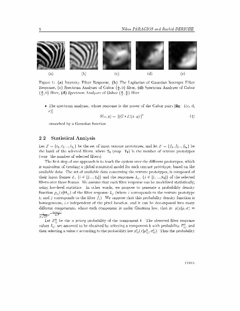
� The intensity �lter, �(x; y) = I(x; y): [�g. 1(a)]

� An isotropic center-surround �lter, which in our case is the Laplacian of Gaussian �lter

(LOG �lter),

F (x; yj�) = S �

�1�

r2

2�2

�e�

r2

2�2 ; r2 = x2 + y2 (2)

where S is a scale factor. Concerning the variance of these �lters, we have � 2

f1; 2; 3; 4; 5g. A response of an isotropic �lter of this form is shown in [�g. 1(b)].

Additionally, this category contains the (x; y) anisotropic directional derivatives �lters.

� Gabor bandpass �lters,

G(x; yj�; �; ) = g(x; yj�)e�j2�(�x+ y) (3)

with �; 2�0; �6 ;

�3 ;

�2 ;

2�3 ;

5�6 ; �; 2�

.

RR n° 3440


(a) (b) (c) (d) (e)

Figure 1: (a) Intensity Filter Response, (b) The Laplacian of Gaussian Isotropic Filter

Response, (c) Spectrum Analyzer of Gabor��6 ; 0

��lter, (d) Spectrum Analyzer of Gabor�

�3 ; 0

��lter, (d) Spectrum Analyzer of Gabor

��3 ;

�6

��lter

� The spectrum analyzer, whose response is the power of the Gabor pairs [�g. 1(c, d,

e)]

S(x; y) = jj(G � I)(x; y)jj2 (4)

smoothed by a Gaussian function.

2.2 Statistical Analysis

Let T = ft1; t2; ::; tTNg be the set of input texture prototypes, and let F = ff1; f2::; fFNg be

the bank of the selected �lters, where TN (resp. FN) is the number of texture prototypes

(resp. the number of selected �lters).

The �rst step of our approach is to teach the system over the di�erent prototypes, which

is equivalent of creating a global statistical model for each texture prototype, based on the

available data. The set of available data concerning the texture prototypes, is composed of

their input frames Ii, fi 2 [1:::; TN]g and the responses Iij , fj 2 [1; :::; FN]g of the selected

�lters over these frames. We assume that each �lter response can be modelized statistically,

using low-level statistics. In other words, we propose to generate a probability density

function pij(xj�ij) of the �lter response Iij (where i corresponds to the texture prototype

ti and j corresponds to the �lter fj). We suppose that this probability density function is

homogeneous, i.e independent of the pixel location, and it can be decomposed into many

di�erent components, where each component is under Gaussian law, that is: p(xj�; �) =

1�p2�e�

(x��)2

2�2 .

Let P kij be the a priory probability of the component k. The observed �lter response

values Iij , are assumed to be obtained by selecting a component k with probability P kij , and

then selecting a value x according to the probability law pkij(xj�kij ; �

kij). Thus the probability

INRIA


(a) (b) (c) (d)

Figure 2: Mixture Analysis for [�g. 1.c] (Spectrum Analyzer of (�6 ; 0) Gabor �lter)

Solid Line: Samples, Dashed Line: Probability Density Functions.

(a) One Component, Mean Approximation Error: 7.3861e-05, Maximal: 0.0039875

(b) Two Components, Mean Approximation Error: 4.3575e-05, Maximal: 0.0034018

(c) Three Components, Mean Approximation Error: 4.184e-05, Maximal: 0.0028997

(d) Four Components, Mean Approximation Error: 4.1353e-05, Maximal: 0.003001

density function is given by

pij(xj�ij) =CNXk=1

P kijpkij(xj�

kij ; �

kij) (5)

where CN is the number of mixture components, and �ij is the vector of the unknown

mixture synthesis parameters: �ij = f(P kij ; �kij ; �

kij) : k 2 [1; :::; CN ]g. Under this hypothesis

there are two key problems: the number of di�erent components CN , and the estimation of

the unknown parameters �ij of these components. Concerning the number of components,

experimentally in most of the cases it has been found to be equal to two, but there are

some cases where at least three components must be assumed. This case appears very

often for textures prototypes which are not quite homogeneous. The determination of the

components number is based on the mean approximation error between the given samples

and the mixture approximation, in other words we increment the number of components

until the mean approximation error drops down from a given threshold. Concerning the

example of [�g. (2)], the improvement of the approximation between the use of two and three

components is not signi�cant, thus we approximate this �lter response with two components.

The estimation of the unknown parameters �ij is obtained using a well known non-linear

minimization method, the Levenberg-Marquardt algorithm [26].

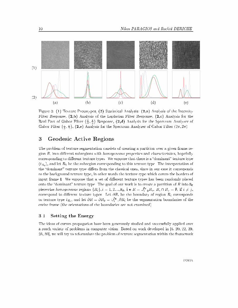
This operation is applied over the set of di�erent �lters responses. This permits us

to create a vector of probability density functions pi = (pi1; pi2; :::; piFN ), for the texture

prototype ti. The same operation is applied for every texture prototype, and as an output

we determine a multi-valued statistical representation of each prototype (see [�g. (3)].

RR n° 3440


(1)

(2)

(a) (b) (c) (d) (e)

Figure 3: (1) Texture Prototypes, (2) Statistical Analysis: (2,a) Analysis of the Intensity

Filter Response, (2,b) Analysis of the Laplacian Filter Response, (2,c) Analysis for the

Real Part of Gabor Filter��3 ;

�2

�Response, (2,d) Analysis for the Spectrum Analyzer of

Gabor Filter��3 ;

�2

�, (2,e) Analysis for the Spectrum Analyzer of Gabor Filter (2�; 2�)

3 Geodesic Active Regions

The problem of texture segmentation consists of creating a partition over a given frame re-

gion R, into di�erent subregions with homogeneous properties and characteristics, hopefully

corresponding to di�erent texture types. We suppose that there is a �dominant� texture type

(tR0), and let R0 be the subregion corresponding to this texture type. The interpretation of

the �dominant� texture type di�ers from the classical ones, since in our case it corresponds

to the background texture type, in other words the texture type which covers the borders of

input frame I. We suppose that a set of di�erent texture types has been randomly placed

onto the �dominant� texture type. The goal of our work is to create a partition of R into RN

piecewise homogeneous regions fRig; i = 1; 2; ::; RN, i.e R = [RN

i=0Ri; Ri \ Rj = ;, if i 6= j,

correspond to di�erent texture types. Let @Ri be the boundary of region Ri corresponds

to texture type tRi , and let @R = @R0 = [RN

i=1@Ri be the segmentation boundaries of the

entire frame (the orientations of the boundaries are not examined).

3.1 Setting the Energy

The ideas of curves propagation have been generously studied and successfully applied over

a reach variety of problems in computer vision. Based on work developed in [8, 20, 22, 29,

28, 30], we will try to reformulate the problem of texture segmentation within the framework

INRIA


of curve evolution theory, by proposing a new model called Geodesic Active Regions.

Let E(@R) be the objective function to be minimized. The classic geodesic active contour

model consists of minimizing

E(@R) =

RNXi=1

�

Z 1

0

j@ Ri(pi)j2dpi| {z }

term1

+

Z 1

0

g2(jrI(@Ri(pi))j)dpi| {z }term2

(6)

where @Ri(pi) : [0; 1]! R2 is a parameterization of the region boundary Ri in a planar form,

and f�; g are real positive constants. The �rst energy component accounts for the expected

spatial properties (i.e. smoothness) of the contour while the second energy component stands

for the attraction energy term of the curve towards the objects contour. Finally, g is a

monotonically decreasing function such that g(r); 0 as r ;1 and g(0) = 1.

Following the work of [3, 7], it can be proved that the minimization of (6) leads to a

geodesic curve with a new metric,

E(@R) = �

RNXi=1

Z 1

0

g(jrI(@Ri(pi))j)j@ Ri(pi)jdpi (7)

where � is a positive constant.

It is well known that in the case of texture segmentation, the edges don't always corre-

spond to region boundaries, thus if one wants to take into account the texture information,

the function g(:) must be replaced. Let h : R2 ! R be an alternative selection of function

g(:), with values close to zero over the regions boundaries, and close to one otherwise.

3.1.1 Setting the Energy Using "texture-boundary" Measurements

The de�nition of function h(:) for the case of texture frames is a quite interesting step. The

role of function h(:) is to incorporate the available texture edge-boundary information. It

is quite obvious that in the case of texture images the gradient features don't rely always

to real boundary edges. In order to obtain these features we try to design a local operator

which neither selects the �best� observed frame, neither uses the entire set of the observed

frames, and gives a measure of the likelihood of a pixel lying on the boundary between the

dominant texture region and another texture region. We propose two di�erent methods,

one which makes use of a single frame and a second method which makes use of several

di�erently parametric images or images from di�erent modalities.

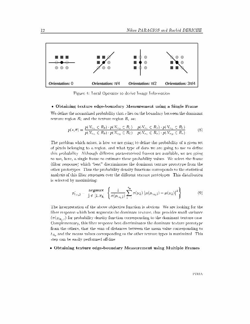
Let s be a pixel in the image grid. At each pixel s, a small neighborhood is de�ned [�g.

4]. Now, given a possible boundary point s and a direction �, the neighborhood is divided

into parts Nsl and Nsr . Concerning the di�erent orientations �, four di�erent possible

directions are assumed, � =�0; �4 ;

�2 ;

3�4

.

RR n° 3440


Orientation: Orientation: Orientation: Orientation: 0 π/2π/4 3π/4

Figure 4: Local Operator to derive Image Information

� Obtaining texture edge-boundary Measurement using a Single Frame

We de�ne the normalized probability that s lies on the boundary between the dominant

texture region R0 and the texture region Rr as:

p(s; �) =p(NsL 2 R0) � p(NsR 2 Rr) + p(NsL 2 Rr) � p(NsR 2 R0)

p(NsL 2 R0) � p(NsR 2 R0) + p(NsL 2 Rr) � p(NsR 2 Rr)(8)

The problem which arises, is how we are going to de�ne the probability of a given set

of pixels belonging to a region, and what type of data we are going to use to de�ne

this probability. Although di�erent parameterized frames are available, we are going

to use, here, a single frame to estimate these probability values. We select the frame

(�lter response) which �best� discriminates the dominant texture prototype from the

other prototypes. Thus the probability density functions corresponds to the statistical

analysis of this �lter responses over the di�erent texture prototypes. This distribution

is selected by maximizing:

p�tR0 j =argmax

j 2 [1; FN]

(1

�(ptR0 j)

TNXi=1

�(pij)��(ptR0 j)� �(pij)

�2)(9)

The interpretation of the above objective function is obvious. We are looking for the

�lter response which best segments the dominant texture, that provides small variance

(�(ptR0 j ) for probability density function corresponding to the dominant texture case.

Complementary, this �lter response best discriminates the dominant texture prototype

from the others, that the sum of distances between the mean value corresponding to

tR0 and the means values corresponding to the other texture types is maximized. This

step can be easily performed o�-line.

� Obtaining texture edge-boundary Measurement using Multiple Frames

INRIA


Let xi(sl) (resp. xi(sr)) be the mean neighborhood value of Nsl (resp. Nsr ) for the

observed frame Ii: the response of �lter fi. Since several di�erently parametric frames

are available, we can estimate the vector x(sl) = [x1(sl); :::; xFN(sl)] (resp. x(sr)).

Based on the texture statistical model (explained in the previous Section), we can

estimate for a given neighborhood region (with observation data set x) the probability

vector corresponding to each texture prototype, thus we generate the matrix

P (x) =

264

p1(x)...

pTN(x)

375 =

264

p11(x1) ... p1FN(xFN)...

......

pTN1(x1) ... pTNFN(xFN)

375

| {z }FN�TN

(10)

Now given a point s, a partition over the neighborhood (Nsl ; Nsr ), and its correspond-

ing data vectors (x(sl);x(sr)), we de�ne the probability that s lies on the boundary

between the dominant texture region R0 and the texture region Rr using a correlation

criterion, as the dissimilarity between the two corresponding probability vectors :

p(s; �) =jjptR0 (x(sl))� ptRr (x(sr))jj

2

jjptR0 (x(sl))jj2 + jjptRr (x(sr))jj

2+

jjptRr (x(sl))� ptR0 (x(sr))jj2

jjptR0 (x(sl))jj2 + jjptRr (x(sr))jj

2(11)

wherejjpm(x)� pn(y)jj2

jjpm(x)jj2 + jjpn(y)jj2=

PFN

j=1[pmj(xj)� pnj(xj)]2P

FN

j=1 pmj(xj)2 +

PFN

j=1 pnj(yj)2

(12)

The correlation scores are computed by comparing the corresponding probability vec-

tors between the texture prototypes tR0 and tRr . Supposing that we are in the bound-

aries of a texture region, then the correlation between the probability vectors of tR0

and tRr is very bad, thus the probability that s lies on the boundary goes to one.

Since the probability that s lies on the boundary between the dominant texture region

R0 and the texture region Rr is de�ned for both cases, the next problem is to de�ne the

texture prototype t�r corresponding to the region Rr, as well as the orientation ��. The best

way to select t�r as well as the orientation �� is to generate the matrix

PEDGE(t; �) =

26666666664

p(0; t1) p(�4 ; t1) p(�2 ; t1) p( 3�4 ; t1)...

......

...

p(0; ttR0�1) p(�4 ; ttR0�1) p(�2 ; ttR0�1) p( 3�4 ; ttR0�1)p(0; ttR0+1) p(�4 ; ttR0+1) p(�2 ; ttR0+1) p( 3�4 ; ttR0+1)

......

......

p(0; tTN) p(�4 ; tTN) p(�2 ; tTN) p( 3�4 ; tTN)

37777777775

(13)

RR n° 3440


(a) (b) (c)

Figure 5: (a) Input frame (b) Texture edge-boundary features extraction using a single

frame, (c) Texture edge-boundary features extraction using multiple frames

and t�r , �� correspond to the biggest element in matrix P . Thus for each point s = (x ; y)

the �edge� features [�g. 5] are captured by the function h(:):

h(s) = e�p[��(s);t�r(s)] (14)

Motivated by work proposed in [7] we can rewrite the geodesic active contour equation

as:

E(@R) = �

RNXi=1

Z 1

0

h(@Ri(pi))j@ Ri(pi)jdpi (15)

where the texture edge-based features have been incorporated to the model.

3.1.2 Setting the Energy Using Region-based Measurements

The main goal of region-based segmentation methods is to classify a particular texture frame

into a number of regions. Thus for each pixel in the image, we need somehow to decide or

estimate which class it belongs to. There is a variety of approaches to do region based

segmentation, but most of them are �nally turn out to be minimization of objective-cost

functions. Usually these objectives-costs functions consist of two di�erent terms. One,

which express the expected spatial properties (homogeneity of the segmentation map), and

a second which express the adequacy between the segmentation map and the observed data.

An important advantage in our case comes from the fact that we have an idea concerning

the elements which have to be segmented, based on the statistical analysis over the di�erent

texture prototypes. This means that we can de�ne the adequacy term between the observed

data and the segmentation maps

INRIA


Guided by the way of de�ning these objective functions for Markov Random Fields and

avoiding the term which express the hypothesis of homogeneity, for our texture segmentation

problem we de�ne the objective function as:

E(R) = �

RNXi=0

Z ZRi

FNXj=1

wj log�ptRij(Ij(x; y))

�dxdy (16)

where Ij is the response of �lter fj over the input frame, � is a negative constant, and wj are

positive weight constants. The above equation has a simple interpretation. Supposing that,

for a given point (x; y) the proper decision has been taken. This means that the probability

values ptRij(Ij(x; y)) for each �lter response support this decision. These probability values

have to be closed to one, thus the function log�ptRij(Ij(x; y))

�gives a very small negative

value, which is multiplied by �, gives a small positive value. On the other hand if a wrong

decision has been taken the corresponding probability values are closed to zero, and the

function log�ptRij(Ij(x; y))

�gives very big negative values, which multiplied by �, charge

the objective function excessively.

3.1.3 Geodesic Active Regions: The Energy Integration

Motivated by the excellent work proposed in [9, 36, 37], and following our previous work on

tracking using geodesic active contours [29, 28, 30] and tracking using classical snakes and

region information [4], we incorporate the two di�erent segmentation models, by de�ning

an objective function as an improved geodesic active contour model:

E(@R) =

�

RNXi=1

Z 1

0

h(@Ri(pi))j@ Ri(pi)jdpi| {z }Boundary Finding Term

+�

RNXi=0

Z ZRi

FNXj=1

wj log�ptRij(Ij(x; y))

�dxdy

| {z }SegmentationTerm

(17)

The above equation has a simple interpretation. The region segmentation is obtained by

minimizing two kind of �energy terms�. The �rst one (Boundary Finding) gives a minimal-

length smoothed curve over the region boundaries, while the second one (Segmentation)

minimizes the objective function inside this region, by supposing homogeneity. Concerning

the boundary of the dominant texture (@R0), it doesn't appear in the objective function

because it corresponds to the union of the other Regions Boundaries (the orientation is

di�erent). The optimization problem can be reformulated as

E(@R) = �

Z ZR0

FNXj=1

wj log(ptR0j(Ij(x; y))dxdy

+

RNXi=1

8<:�

Z 1

0

h(@Ri(pi))j@ Ri(pi)jdpi + �

Z ZRi

8<:

FNXj=1

wj log(ptRij(Ij(x; y))dxdy

9=;9=; (18)

RR n° 3440


Although the objective function (18) is well-de�ned, there are still some unknown vari-

ables. We want to minimize this function over the region boundaries, and as an output we

would like to obtain also the region segmentation. In order to do this, as it is quite clear

from the de�nition of the objective function, we need a correspondence between the regions

Ri and texture prototypes tRi something which we don't have a priory. This problem is

going to be confronted later (Subsection 3.2).

3.2 Minimizing the Energy

Finally, the objective function is minimized using a steepest gradient descend method. Let

~u = (x; y) be a point of the initial curve. We compute the Euler-Lagrange equations 1 , and

according to them, in order to deform each point ~u of the initial curve towards the local

minima of the objective function [8],we should use the following equation:

d~u

dt= �

8<:

FNXj=1

wj log(pj(Ij(~u)))

9=; ~N@R0(~u)+

1The following nice development can be found in [36, 37]. The problem of taking functional derivatives

of integrals along contours and integrals over regions can be confronted using Green's theorem, which is a

special case of Stokes theorem.Consider

E[@R] =

Z ZR

f(x; y)dxdy

where @R = (x(s); y(s)) is the boundary of the contour of region R, with 0 � s � l is the arc-length. Greens

theorem states that: for a planar region R, (P (x; y); Q(x; y)) is any vector �eld with continuous �rst order

derivatives, then Z ZR

�@Q

@x�

@P

@x

�dxdy =

Z@R

Pdx+Qdy =

Z l

0

(P x+Q y)ds

where x, y denotes the di�erentiation with respect to s. Let Q(x; y) = 12

R x0f(t; x)dt and P (x; y) =

� 12

R y0f(x; t)dt. In that case @Q

@x� @P

@x= f(x; y), thus

E[@R] =

Z ZR

f(x; y)dxdy =

Z l

0

L(x; x; y; y)ds

where L(x; x; y; y) = Q(x; y) x + P (x; y) y. By Euler-Lagrange equation, we get the gradient of E[@R] with

respect to any point (x(s); y(s)) 2 @R we have:

�E

�x=

@E

@x�

d

ds

@L

@ x= ::: = f(x; y) y ;

�E

�y=

@E

@y�

d

ds

@L

@ y= ::: = �f(x; y) x

and since ~N(x;y) = ( y;� x) is the normal along the contour, by setting ~u = (x; y) we have

�E

�u= f(x; y) ~N(x;y)

INRIA


��h(~u)K@Rr (~u) +rh(~u) � ~N@Rr (~u))

�~N@Rr(~u) + �

8<:

FNXj=1

wj log(pj(Ij)(~u))

9=; ~N@Rr (~u) (19)

where r is the index of the region in which the point ~u belongs, K@Rr is the Euclidean

curvature with respect to the curve @Rr and N@Rr is the unit inward normal to @Rr. Since

the curves @R0 and @Rr have inverse inwards vectors at each common point ~u, we have~N = ~NRr = � ~NR0 . Taking this into account and replacing KRr by K, the motion equation

for ~u can be rewritten as:

d~u

dt=

0BBBBB@�

hh(~u)K(~u) +rh(~u) � ~N (~u))

i| {z }

Boundary Finding Forces

+�

24 FNXj=1

wj logptRr j(Ij(~u))

ptR0j(Ij(~u))

35

| {z }Statistics Region Forces

1CCCCCA ~N (~u)) (20)

The obtained motion equation has a quite obvious interpretation. There are two kind of

�forces� acting on the contour, both in the direction of the inward normal. The �rst term, is

a contour force which contains information regarding the boundaries of the di�erent region

areas. This term takes into account the boundary image characteristics, and at the same

time is a smoothing force, since its value depends on the curvature term. The second term is

a statistic-region force. We will try to interpret this term. Supposing that ~u is a pixel of the

dominant texture font. In such a case the input data I as well as the responses of the �lter

bank Ij , must support the hypothesis R0, thus ptR0j(Ij(~u)) > ptij(Ij(~u)), 8 ti 6= tR0 . The

in�uence of the statistics region forces, now is quite evident. In the case where the observed

multi-value data at ~u �ts better to the dominant texture �log

�ptRr j

(Ij(~u))

ptR0 j(Ij(~u))

�> 0, 8 tRi we

are going to compresses the region, otherwise we are going to expand the region. This is a

very nice property, since the contour can evolve either inwards, either outwards at the same

time for di�erent pixel sites. This is possible due to the fact that the contour propagation

is guided by a speed function which is either positive, either negative, and is estimated

according to the observed data. Opposite to this, on the classic geodesic active contour

model we don't meet this property, since we have negative speed values only because of

the curvature e�ect. As a consequence, the contour initialization doesn't pose signi�cant

problems.

Finally, the problem of correspondence regions and texture prototypes in not solved yet.

Giving a second look on the motion equation (20), we can see that the term of textures-

regions correspondence appears only in the statistics force, which is estimated locally. Taking

this into account, the textures-regions correspondence is obtained by maximizing the statistic

force. In other words for each point of the given boundaries we compare the dominant

texture hypothesis, with the texture hypothesis which �ts better with the observed data on

this point.

RR n° 3440


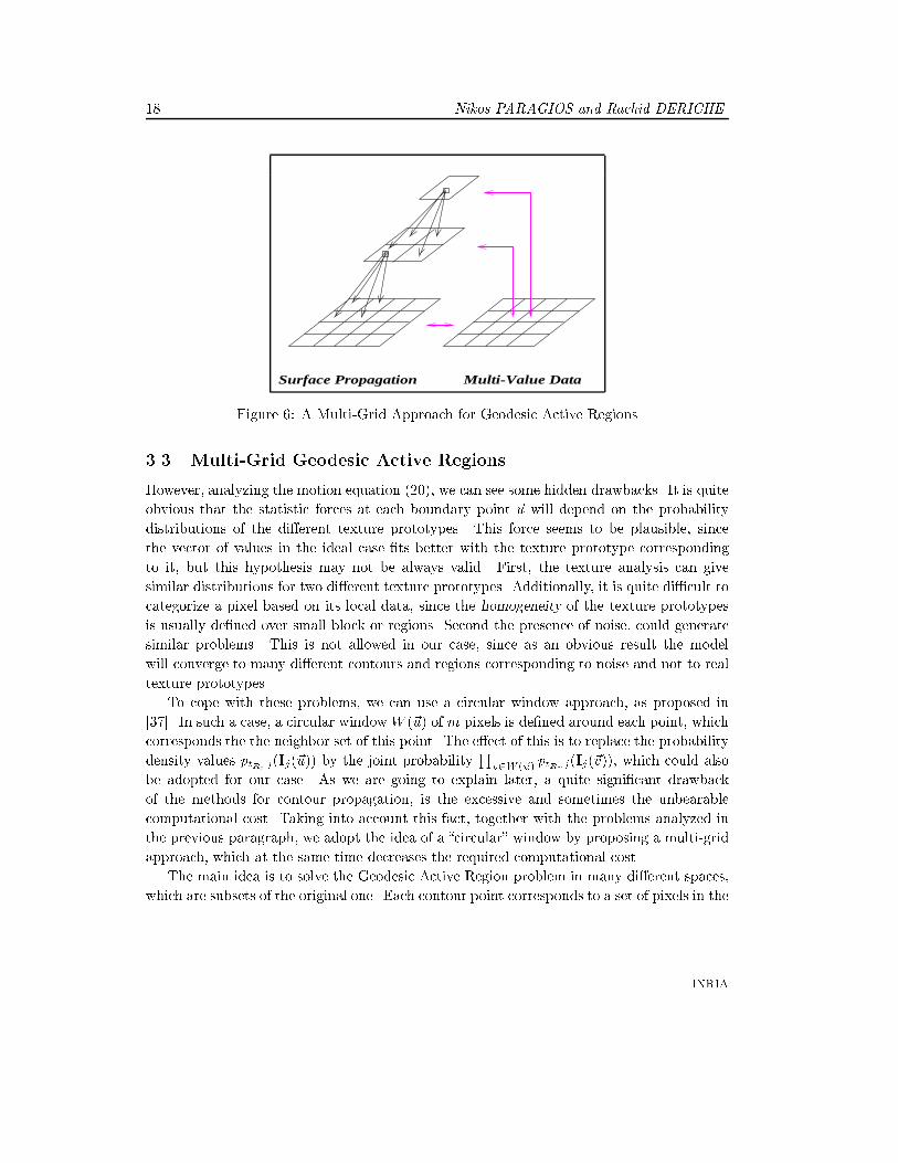
Surface Propagation Multi-Value Data

Figure 6: A Multi-Grid Approach for Geodesic Active Regions

3.3 Multi-Grid Geodesic Active Regions

However, analyzing the motion equation (20), we can see some hidden drawbacks. It is quite

obvious that the statistic forces at each boundary point ~u will depend on the probability

distributions of the di�erent texture prototypes. This force seems to be plausible, since

the vector of values in the ideal case �ts better with the texture prototype corresponding

to it, but this hypothesis may not be always valid. First, the texture analysis can give

similar distributions for two di�erent texture prototypes. Additionally, it is quite di�cult to

categorize a pixel based on its local data, since the homogeneity of the texture prototypes

is usually de�ned over small block or regions. Second the presence of noise, could generate

similar problems. This is not allowed in our case, since as an obvious result the model

will converge to many di�erent contours and regions corresponding to noise and not to real

texture prototypes.

To cope with these problems, we can use a circular window approach, as proposed in

[37]. In such a case, a circular windowW (~u) of m pixels is de�ned around each point, which

corresponds the the neighbor set of this point. The e�ect of this is to replace the probability

density values ptRr j(Ij(~u)) by the joint probabilityQv2W (~u) ptRr j(Ij(~v)), which could also

be adopted for our case. As we are going to explain later, a quite signi�cant drawback

of the methods for contour propagation, is the excessive and sometimes the unbearable

computational cost. Taking into account this fact, together with the problems analyzed in

the previous paragraph, we adopt the idea of a �circular� window by proposing a multi-grid

approach, which at the same time decreases the required computational cost.

The main idea is to solve the Geodesic Active Region problem in many di�erent spaces,

which are subsets of the original one. Each contour point corresponds to a set of pixels in the

INRIA


original space. A quite sophisticated approach consists in de�ning a consistent multi-grid

contour propagation model by using contours which are constrained to be piecewise constant

over smaller and smaller pixel subsets [15]. The objective function which is considered

at each level is then automatically derived from the original �nest scale energy function,

as well as the partial di�erential equation which deforms the initial contour. Also, full

observation space is used at each contour level and there is no necessity for constructing a

multi-resolution pyramid of the data [�g. 6]. Correspondingly for the level L, we obtain a

generalized objective function:

E(@RL) = �

RNXi=1

Z 1

0

hL(@RLi (pi))j@ R

L

i (pi)jdpi+

�

RNXi=0

Z ZRLi

8<:

FNXj=1

wj1

jWL(x; y)j

Z Z(u;v)2WL(x;y)

loghpt

@RL0j(Ij(u; v))

idudv

9=; dxdy (21)

where @RLi is the boundary of region RLi (corresponds to level L), WL(x; y) the window in

full data space corresponding to the point (x; y) of data space at level L, and

hL(@RLi (pi)) =

1��WL(@RLi (pi))��sZ Z

(x;y)2WL(@RLi(pi))

h2(u; v)dudv

The multi-resolution approach solves our problems. At low resolution levels a block of

data points is used to move the boundary points, thus the chance to be representative in

terms of the texture prototype are quite bigger. On the other hand, at these low resolution

levels the size of the window is quite big and the boundary is not located precisely. This is

not a problem since moving from the low resolution to the high resolution levels, the window

size gets smaller and smaller, and the statistics forces moving the boundary points are more

accurate. Additionally at low resolution level, we have obtained a segmentation where the

noise in�uence has been removed, and since this result is used to initialize the operation at

the next level we don't have the problems mentioned above.

3.4 Level Set Implementation

The motion equation (20) could be implemented using a Lagrangian approach, where we

produce equations of motion for the position vector @R(p; t), and then updating these posi-

tion using di�erence approximation scheme. However, there are several problems with this

approach. The main problem is that the evolving model is not capable to deal with topo-

logical changes of the moving front. Additionally, this method cannot be easily extended to

three dimensions.

RR n° 3440


This could be avoided by introducing the work of Osher and Sethian [27]. The central

idea is to represent the moving front @R(t) as the zero-level set f� = 0g of a function �.

This representation of @R(t) is implicit, parameter-free and intrinsic. Additionally, it is

topology-free since di�erent topologies of the zero level-set do not imply di�erent topologies

of �. It easy to show, that if the moving front evolves according to

d

dt@R(p; t) = F(p) ~N

for a given function F , then the embedding function � deforms according to

d

dt�(p; t) = F(p) jr�(p; t)j

For this level-set representation, it is proved that the solution is independent of the embed-

ding function �, and in our case is initialized as a signed distance function. Based on (18)

and embedding (20) in � we obtain that minimizing the Geodesic Active Region Function

is equivalent to searching a steady-state solution of the following equation:

d�

dt=

0@� [hK +rh � r�] + �

24 FNXj=1

wj logptRr j(Ij)

ptR0j(Ij)

351A jr�j (22)

where the @R(p; t) is represented by a level-set of � and the value of K is estimated on �,

K = div(r�=jr�j).

4 Front Propagation Algorithms

A direct implementation approach of equation (22) involves the re-estimation of the char-

acteristic image of all the level set pixels (not simply the zero level set corresponding to

the front itself). This front evolution method is computationally very expensive, due to

many useless operations that are performed during the front propagation (especially in pix-

els which are out of interest). In order to overcome this drawback two di�erent methods

have been proposed: (i) the �Narrow Band� method that works with a small percentage of

pixels (those which are around to the latest estimation of the contour) [2], (ii) the �Hermes�

method, a fast approach suitable to a large variety of applications [28].

4.1 Narrow Band Approach

The key idea is to deal only with pixels which are close to the latest estimation of the zero

level-set contour in both directions (inwards and outwards). This is known as Narrow Band

Approach [2], and proposes to modify the level-set method so that it only a�ects the points

INRIA


close to the current propagating contour. This band is created dynamically based on the

actual propagating contour, by including points that lie less than some given distance away

from the actual contour points (band size). The problem is that the contour position changes

dynamically (from iteration to iteration), as well as the narrow band pixels. The estimation

of the contour position from iteration to iteration increases dynamically the cost (in terms

of complexity), thus the contour position is re-estimated only in cases where the contour is

very close to the borders of the band. The selection of the band size a�ects signi�cantly

the e�cacy of this algorithm. A signi�cant cost reduction is achieved through this approach

(compared to the classic method), but the cost remains considerable.

4.2 Hermes Algorithm

Hermes algorithm was originally proposed in [28], and tries to combines two well-known

level-set algorithms, the Narrow Band and the Fast Marching [34]. Despite the fact that

Fast Marching is a very fast algorithm, it cannot be used for our case since it demands a

curve which evolves using an only positive or negative speed function during its evolution.

In our case this is not-valid, because of the region-statistics forces. As it is explained, these

forces shrink the curve if it is located on the dominant texture region, otherwise they expand

it.

The main characteristic of Hermes algorithm is that it proposes a fast way to deform the

initial curve towards the global minimum of the objective function. In our case the equation

which deforms the initial curve (22) can be rewritten in a more general form as:

�t+1(x;y) = �t

(x;y) + V(x; y;�)dt (23)

where V(x; y;�) is the speed function, depending on geometric features (curvature) and

image features (�edge-based� forces and �region-based� forces). Since the speed V(x; y;�) is

basically estimated according to image characteristics, there are some points for which the

front evolves faster compared to the others. The key idea on which Hermes approach is

based, is to evolve the contour according to the speed values of its points. The algorithm at

each step selects the point with the biggest speed from a set of actual contour points, and

deforms the level-set frame locally.

First we initialize the contour and we set both the contour points and their neighbors

as active. We select from the set of active points the one with the biggest speed and we

iteratively modify the level-set frame for this point as well as for its neighborhood using

(23). This operation is applied for a certain number of iterations. Since there are modi�ed

level-set frame values, there are some a�ected active points (in terms of curvature), as well as

some a�ected neighborhood points which are not active, that we add to the set of active. If

the level-set value of the selected point changes sign, which means that the contour deforms

locally, we remove this point from Active ones. Periodically we �nd the contour position

RR n° 3440


in order to avoid the creation of a large set of Active pixels and we reinitialize the level-

set frame using a distance function, since this frame is partially modi�ed. Concerning the

neighborhood de�nition we use a 5� 5 centralized window, while the number of the locally

applied iterations varies between 10 and 50. Both parameters a�ect drastically the CPU

computational cost.

The key issue for an e�cient version of the Hermes algorithm lies on a fast way of locating

the grid point among the Active points with the biggest speed. For this reason, a variation

of a heap-sort algorithm is used. Initially all the narrow points are sorted in a heap-sort

(so that the smallest member can be easily located). When a point is removed from the

heap-sort, the values of its neighbors are recomputed, and the results are bubbled upwards

until they reach their correct locations. Moreover, whenever we want to add a point to the

heap-sort, we put it at the end and we process it in the same way.

5 Experimental Results, Conclusions and Discussion

In this paper, we presented some new ideas concerning the integration of boundary-�nding

techniques and region-based approaches for texture segmentation.

5.1 Implementation Issues

Although we proposed a complete model, there are some technical aspects which a�ects its

e�ciency. These aspects consist of: the �lter bank selection, the number of multi-grid levels,

the contour initialization, and the Level-Set algorithm selection. We will try to give an idea

of how we deal with these aspects.

� Filters Bank Determination

This problem involves the de�nition of the Filter Bank, which includes three aspects:

the �lters number, their selection, and their size. We can say that the �rst two problems

are strongly related. It is quite obvious that a �good� selection of �lters decreases their

required number to discriminate the texture prototypes. Experimentally, we could say

that in most of the cases, we use �ve or six �lters, but these �lters are manually selected

to be optimal, i.e. to extract features which are clearly discriminated between the

di�erent prototypes. The �lter size holds an important role on the features extraction

process. The texture homogeneity cannot be captured using a small window, since

this homogeneity appears in the forms of repeated �patterns�. On the other hand a

big �lter size creates problems between the boundaries of di�erent texture regions and

makes their localization quite problematic in terms of accuracy. Experimentally the

�lter size is selected to be 10� 10 or 15� 15.

INRIA


� Multi-grid Levels

The selection of multi-grid levels is strongly related to the size of the input frames,

in terms of the pyramid compensation cost. Since this approach is not based on the

construction of a frame pyramid, we can easily go to very low resolution levels. This is

possible due to the use of the full data observation space in each level. Experimentally,

in most of the cases, this number is selected to be either three or four.

� Contour Initialization

The contour initialization is low-risk step. Supposing that the dominant texture is

known, then we can initialize the contour at the borders of the input frame, and the

proposed model will deform it towards the global minimum of the objective function

[�g. (7,8,10,12)]. Additionally the model, deforms successfully contours which have

been initialized randomly, towards the global minimum of the objective function [�g.

(9,11,13)]. This is achieved thanks to the region-statistics forces which deform the con-

tour outwards to regions di�erent from the dominant one. This �random� initialization

supposes that a part of each texture prototype appears in the region inside the initial

contour.

� Level-Set Propagation Algorithm

The selection of the Level-Set implementation algorithm is not a crucial step. Concern-

ing the Narrow Band approach, it converges smoothly towards the optimal solution,

but it is time consuming. On the other hand, Hermes algorithm deforms faster the

initial contour towards the optimal solution, but it doesn't ensure a smooth propaga-

tion since the Level-Set frame at each step is updated locally. As a consequence the

Level-Set frame re�nement must be performed quite often.

5.2 Experimental Results

Real-word texture frame, as well synthetic texture frames have been used to test and validate

the proposed approach.

Concerning the synthetic case some texture prototypes have been selected from a database

of texture images. As a �rst step the system is taught on these prototypes by applying the

bank of preselected �lters, and analyzing their responses. The output of this operation is

the creation of a global statistical description model for each prototype. Then a synthetic

frame is created where regions of the selected texture prototypes appear randomly. This is

considered as the input frame, on which the same bank of preselected �lters is applied. Then

using the di�erent �lter responses, as well as the texture description models, the Geodesic

Active Region models is activated, and deforms the initial curve to the optimal solution of

the texture segmentation problem.

RR n° 3440


The �rst experimental result [�g. (7)] involves a texture synthesis frame composed of

two quite di�erent prototypes (in terms of intensity distributions). As a consequence, the

number of required �lters is small, and the segmentation process is easily performed. On the

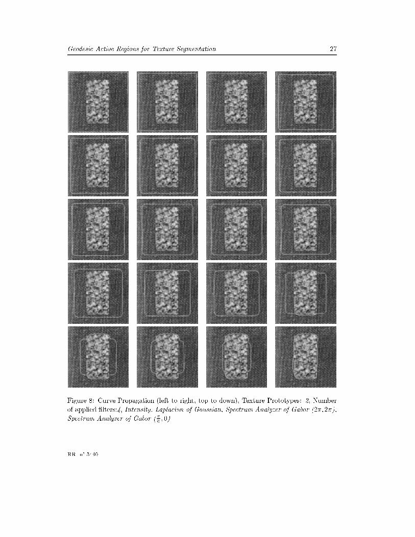
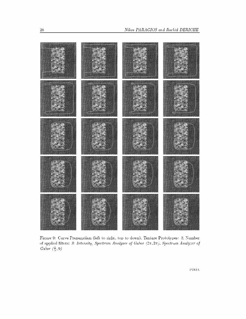
contrary, the second example [�g. (8,9)] involves a texture synthesis frame with two quite

similar prototypes (in terms of intensity distributions). Additionally, the non-dominant

texture prototype is not quite homogeneous (in terms of a repeated pattern). For this case,

two di�erent contour initializations have been used: the �proper� (at the borders of the input

frame) [�g. (8)], and a random one which contains a part of the dominant texture as well as

a part of the the non-dominant texture [�g. (9)]. As it is shown for this example, the contour

shrinks if it is located in the dominant texture region; otherwise the contour is expanded.

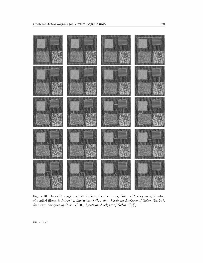
Finally, the last experimental result [�g. (10,11)] involves a texture synthesis frame with �ve

di�erent texture regions, where two di�erent contour initializations are shown. The large

number of di�erent texture regions requires the selection of a representative �lter bank. In

this example, the famous level-set property of changing the topology is demonstrated, where

the initial curve breaks into multiple curves corresponding to the di�erent texture regions.

On the contrary for the real case, the inverse operation is followed since the input is the

real-texture synthesis frame [�g. (12,13,14,15,16)]. Small patterns are selected to represent

the di�erent texture prototypes appearing to this frame, and the system is taught with

these patterns. Then the same process is followed as in the case of synthetic texture frames.

Concerning the �rt �real-world� example that consists two demonstrations (zebra and chita

photos) [�g. (12,13,14)], we select from a 256� 256 textured frame three di�erent window

patterns 64 � 64 (resp. 96 � 96) [�g. 12.1] (resp. [�g. 14.1]) that are the di�erent

texture prototypes, and based on these patterns we activate the Geodesic Active Region

Model which segments quite well the di�erent texture regions. The independence of the

model from the contour initialization is clearly presented using two completely di�erent

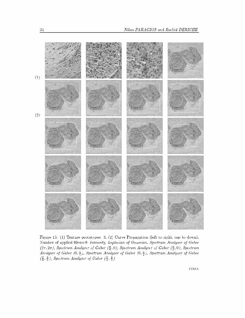
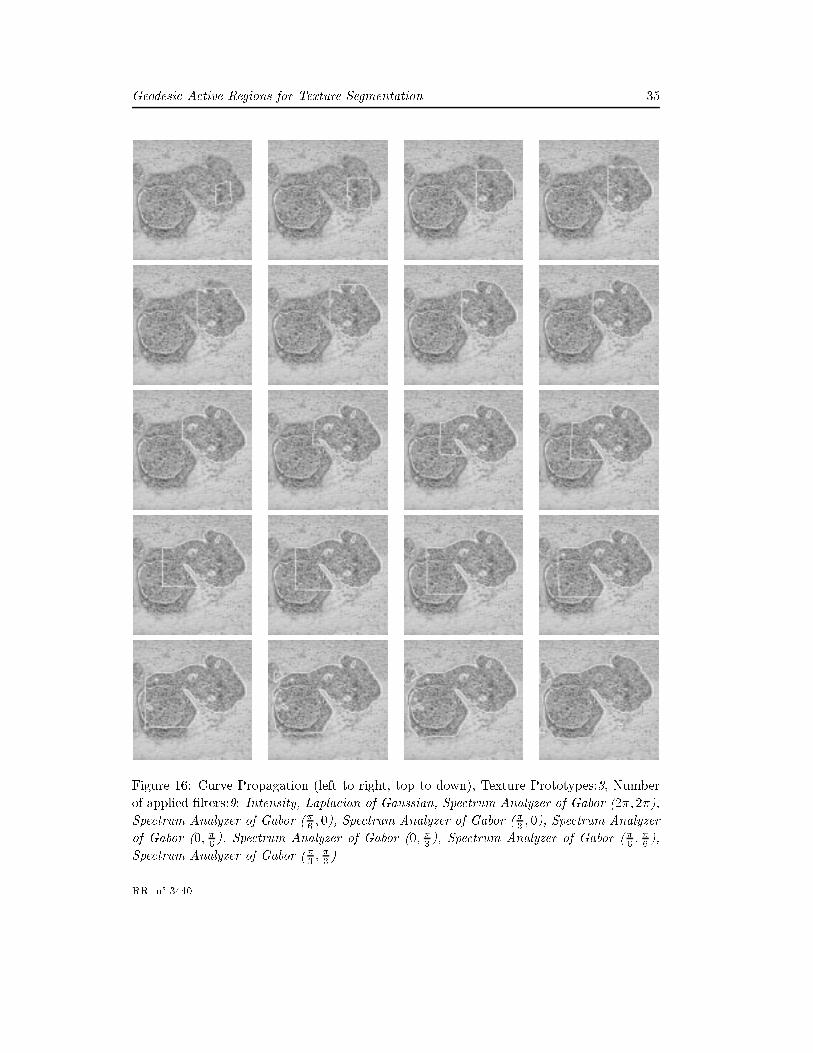
contour initializations. The second �real-world� example related to medicine [�g. (15,16)],

is a microscopic medical breast image, which exhibits an in�ammatory carcinoma with

metastasis. Three di�erent texture patterns have been selected [�g. 15.1], and nine di�erent

�lters have been applied, which give as output the texture description models. The power of

the Geodesic Active Region model is demonstrated using two di�erent contour initializations.

The �rst one is at the borders of the frame [�g. (15)], while the second contains only non-

dominant texture regions [�g. (16)].

5.3 Discussion and Conclusion

Summarizing, we have considered a Contour Propagation approach for texture segmen-

tation. The main contribution of our approach is the Geodesic Active Region Model, a

contour propagation model for texture segmentation, which incorporates the existing

approaches in the domain of texture analysis, as well as in the domain of texture

INRIA


segmentation. Firstly, a global texture description model is generated for each texture

prototype. This model is obtained by fusing �ltering theory and statistical analysis, where

various �lters responses are modelized statistically using mixtures synthesis of Gaussian dis-

tributions. The second step, consists of creating a global segmentation framework, where

region based and boundary �nding techniques are cooperating in a coupled common model.

The contour propagation is obtained by integrating two di�erent modules, region based

module and boundary �nding module in a common model. This leads to a system where the

two modules operate simultaneously, where the contour propagation is guided by smooth-

ing, �edge-based� , and statistics region forces. The main advantage of our model is that

the contour evolves using information not only among it, but also information which come

from the regions inside and outside of it. The changes of topology can be easily obtained

using a Level-Set approach, thereby several texture regions can be detected simultaneously.

The noise presence is confronted multi-grid approach, which simultaneously decreases the

computational cost.

Various experimental results (in MPEG format), including the ones shown in this article,

can be found at:

http://www.inria.fr/robotvis/personnel/nparagio/demos.html

RR n° 3440


Figure 7: Curve Propagation (left to right, top to down), Texture Prototypes:2, Number of

applied �lters:3: Intensity, Laplacian of Gaussian, Spectrum Analyzer of Gabor (2�; 2�)

INRIA


Figure 8: Curve Propagation (left to right, top to down), Texture Prototypes: 2, Number

of applied �lters:4, Intensity, Laplacian of Gaussian, Spectrum Analyzer of Gabor (2�; 2�),

Spectrum Analyzer of Gabor (�6 ; 0)

RR n° 3440


Figure 9: Curve Propagation (left to right, top to down), Texture Prototypes: 2, Number

of applied �lters: 3: Intensity, Spectrum Analyzer of Gabor (2�; 2�), Spectrum Analyzer of

Gabor (�6 ; 0)

INRIA


Figure 10: Curve Propagation (left to right, top to down), Texture Prototypes:5, Number

of applied �lters:5: Intensity, Laplacian of Gaussian, Spectrum Analyzer of Gabor (2�; 2�),

Spectrum Analyzer of Gabor (�6 ; 0), Spectrum Analyzer of Gabor (�2 ;�3 )

RR n° 3440




Spectrum Analyzer of Gabor (�6 ; 0), Spectrum Analyzer of Gabor (�2 ;�3 )

INRIA


(1)

(2)

Figure 12: (1) Texture prototypes, (2) Curve Propagation (left to right, top to down),

Number of applied �lters:6: Intensity, Isotropic Directional Derivatives, Spectrum Analyzer

of Gabor (2�; 2�), Spectrum Analyzer of Gabor (�6 ; 0), Spectrum Analyzer of Gabor (�3 ; 0),

Spectrum Analyzer of Gabor (0; �3 )

RR n° 3440



of applied �lters:6: Intensity, Isotropic Directional Derivatives, Spectrum Analyzer of Gabor

(2�; 2�), Spectrum Analyzer of Gabor (�6 ; 0), Spectrum Analyzer of Gabor (�3 ; 0), Spectrum

Analyzer of Gabor (0; �3 )

INRIA


(1)

(2)

Figure 14: (1) Texture prototypes, (2) Curve Propagation (left to right, top to down), Num-

ber of applied �lters:8: Intensity, Spectrum Analyzer of Gabor (2�; 2�), Spectrum Analyzer

of Gabor (�6 ; 0), Spectrum Analyzer of Gabor (�3 ; 0), Spectrum Analyzer of Gabor (0; �3 )

Spectrum Analyzer of Gabor (0; �6 ), Spectrum Analyzer of Gabor (�6 ;�3 ), Spectrum Analyzer

of Gabor (�3 ;�6 )

RR n° 3440


(1)

(2)

Figure 15: (1) Texture prototypes: 3, (2) Curve Propagation (left to right, top to down),

Number of applied �lters:9: Intensity, Laplacian of Gaussian, Spectrum Analyzer of Gabor

(2�; 2�), Spectrum Analyzer of Gabor (�6 ; 0), Spectrum Analyzer of Gabor (�3 ; 0), Spectrum

Analyzer of Gabor (0; �6 ), Spectrum Analyzer of Gabor (0; �3 ), Spectrum Analyzer of Gabor

(�6 ;�6 ), Spectrum Analyzer of Gabor (�3 ;

�3 )

INRIA




Spectrum Analyzer of Gabor (�6 ; 0), Spectrum Analyzer of Gabor (�3 ; 0), Spectrum Analyzer

of Gabor (0; �6 ), Spectrum Analyzer of Gabor (0; �3 ), Spectrum Analyzer of Gabor (�6 ;�6 ),

Spectrum Analyzer of Gabor (�3 ;�3 )

RR n° 3440


References

[1] Boston, MA, June 1995. IEEE Computer Society Press.

[2] D. Adalsteinsson and J. A. Sethian. A Fast Level Set Method for Propagating Interfaces.

Journal of Computational Physics, 118(2):269�277, 1995.

[3] Gilles Aubert and Laure Blanc-Feraud. An elementary proof of the equivalence between

2d and 3d classical snakes and geodesic active contours. Technical Report 3340, INRIA,

January 1998.

[4] Bénédicte Bascle and Rachid Deriche. Region tracking through image sequences. In

Proceedings of the 5th International Conference on Computer Vision [1], pages 302�307.

Appeared also as an Inria Research Report RR-2439 (Dec. 1994).

[5] A. Bovik, C. Analysis of multichannel narrow-band �lters for image texture segmenta-

tion. IEEE Trans. Signal Processing, 39(9):2025�2043, 1991.

[6] J. F. Canny. A computational approach to edge detection. IEEE Transactions on

Pattern Analysis and Machine Intelligence, 8(6):769�798, November 1986.

[7] V. Caselles, R. Kimmel, and G. Sapiro. Geodesic active contours. In Proceedings of the

5th International Conference on Computer Vision [1], pages 694�699.

[8] Vicent Caselles, Ron Kimmel, and Guillermo Sapiro. Geodesic active contours. The

International Journal of Computer Vision, 22(1):61�79, 1997.

[9] A. Chakraborty, H. Staib, and J. Duncan. Deformable Boundary Finding in Medical

Images by Integrating Gradient and Region Information. IEEE trans.Medical Imaging,

15(6):859�870, 1996.

[10] L.D. Cohen. On active contour models and balloons. CVGIP: Image Undertanding,

53:211�218, 1991.

[11] G. Cross and A. Jain. Markov random �eld texture models. IEEE, PAMI, 5:25�39,

1983.

[12] R. Deriche. Using canny's criteria to derive a recursively implemented optimal edge

detector. The International Journal of Computer Vision, 1(2):167�187, May 1987.

[13] D. Dunn and W. Higgins. Optimal gabor �lters for texture segmentation. IEEE Trans.

Image Processing, 4(7):947�964, 1995.

[14] D. Gabor. Theory of communications. IEE Proceedings, 93(26), 1946.

INRIA


[15] F. Heitz, P. Perez, and P. Bouthemy. Multiscale minimization of global energy functions

in some visual recovery problems. GVGIP: Image Unterstanding, 59:125�134, 1994.

[16] A. Jain and R. Farrokhsia. Unsupervised texture segmentation using Gabor �lters.

Pattern Recognition, 24:1167�1186, 1991.

[17] M. Kass, A. Witkin, and D. Terzopoulos. Snakes: Active contour models. In First

International Conference on Computer Vision, pages 259�268, London, June 1987.

[18] C. Kervrann and F. Heitz. A Markov Random-Field Model-Based Approach to Un-

supervised Texture Segmentation Using Local and Global Spatial Statistics. Image

Processing, 4(6):856�862, June 1995.

[19] A. Khotanzad and J.Y. Chen. Unsupervised Segmentation of Textured Images by Edge

Detection in Multidimensional Features. IEEE, PAMI, 11(4):414�420, April 1989.

[20] S. Kichenassamy, A. Kumar, P. Olver, A. Tannenbaum, and A. Yezzi. Gradient �ows

and geometric active contour models. In Proc. Fifth International Conference on Com-

puter Vision [1].

[21] A. Leonardis, A. Cupta, and R. Bajcsy. Segmentation of range images as the search

for geometric parametric models. The International Journal of Computer Vision,

14(3):253�270, 1995.

[22] R. Malladi, J. A. Sethian, and B.C. Vemuri. Shape modeling with front propagation:

A level set approach. PAMI, 17(2):158�175, February 1995.

[23] S. Mallat. Multiresolution approximations and wavelet orthonormal bases of L2(R).

Trans. Amer. Math. Soc., 315:69�87, 1989.

[24] B.S. Manjunath and R. Chellappa. Unsupervised Texture Segmentation Using Markov

Random Field Models. IEEE, PAMI, 13(5):478�482, May 1991.

[25] J. Mao and A. Jain. Texture classi�cation and segmentation using multiresolution

simultaneous autoregresive models. Pattern Recognition, 25:173�188, 1992.

[26] J.J. More. The levenberg-marquardt algorithm, implementation and theory. In G. A.

Watson, editor, Numerical Analysis, Lecture Notes in Mathematics 630. Springer-

Verlag, 1977.

[27] S. Osher and J. Sethian. Fronts propagating with curvature dependent speed : algo-

rithms based on the Hamilton-Jacobi formulation. Journal of Computational Physics,

79:12�49, 1988.

RR n° 3440


[28] N. Paragios and R. Deriche. A PDE-based Level Set Approach for Detection and

Tracking of Moving Objects. Technical Report 3173, INRIA, France, May 1997.

http://www.inria.fr/rapports/sophia/RR-3173.html.

[29] N. Paragios and R. Deriche. A PDE-based Level Set Approach for Detection and

Tracking of Moving Objects. In Proceedings of the 6th International Conference on

Computer Vision, Bombay,India, January 1998. IEEE Computer Society Press.

[30] Nikolaos Paragios and Rachid Deriche. Detecting multiple moving targets using de-

formable contours. In International Conference on Image Processing, volume II of III,

pages 183�186, Santa-Barbara,California, October 1997.

[31] A. Pentland. Automatic Extraction of Deformable Part Models. The International

Journal of Computer Vision, pages 107�126, 1990.

[32] H.M. Raafat and A.K.C. Wong. Texture Information-Directed Region Growing Al-

gorithm for Image Segmentation and Region Classi�cation. CVGIP, 43(1):1�21, July

1988.

[33] T.R. Reed, H. Wechsler, and M. Werman. Texture Segmentation Using a Di�usion

Region growing technique. Pattern Recognition, 23(9):953�960, September 1990.

[34] J. A. Sethian. A Fast Marching Level Set Method for Monotonically Advancing Fronts.

In Proc. Nat. Ac. Science, volume 93, pages 1591�1694, 1996.

[35] P. Simoncelli, W. Freeman, H. Adelson, and Heeger J. Shiftable multiscale transforms.

IEEE trans. on Information Theory, 38:587�607, 1992.

[36] S.C. Zhu, T.S. Lee, and A.L. Yuille. Region Competition: Unifying Snakes, Region

Growing Energy/Bayes/MDL for Multi-band Image Segmentation. In proc. of 5th In-

ternational Confereence on Computer Vision, Boston, USA, June 1995.

[37] Song Chun Zhu. Statistical and Computational Theories for Image Segmentation, Tex-

ture Modeling and Object Recognition. PhD thesis, Harvad University, January 1996.

[38] Song Chun Zhu and Alan Yuille. Region Competition: Unifying Snakes, Region Grow-

ing, and Bayes/MDL for Multiband Image Segmentation. IEEE Transactions on Pat-

tern Analysis and Machine Intelligence, 18(9):884�900, September 1996.

INRIA

Unité de recherche INRIA Sophia Antipolis2004, route des Lucioles - B.P. 93 - 06902 Sophia Antipolis Cedex (France)

Unité de recherche INRIA Lorraine : Technopôle de Nancy-Brabois - Campus scientifique615, rue du Jardin Botanique - B.P. 101 - 54602 Villers lès Nancy Cedex (France)

Unité de recherche INRIA Rennes : IRISA, Campus universitaire de Beaulieu - 35042 Rennes Cedex (France)Unité de recherche INRIA Rhône-Alpes : 655, avenue de l’Europe - 38330 Montbonnot St Martin (France)

Unité de recherche INRIA Rocquencourt : Domaine de Voluceau - Rocquencourt - B.P. 105 - 78153 Le Chesnay Cedex (France)

ÉditeurINRIA - Domaine de Voluceau - Rocquencourt, B.P. 105 - 78153 Le Chesnay Cedex (France)

http://www.inria.fr

ISSN 0249-6399

geodesic active regions for texture segmentation€¦ · · 2015-07-29geodesic active regions for...

Documents