Geodesic Convolutional Neural Networks on Riemannian Manifolds

Jonathan Masci†∗ Davide Boscaini†∗ Michael M. Bronstein† Pierre Vandergheynst‡

†USI, Lugano, Switzerland ‡EPFL, Lausanne, Switzerland

Abstract

Feature descriptors play a crucial role in a wide range

of geometry analysis and processing applications, includ-

ing shape correspondence, retrieval, and segmentation. In

this paper, we introduce Geodesic Convolutional Neural

Networks (GCNN), a generalization of the convolutional net-

works (CNN) paradigm to non-Euclidean manifolds. Our

construction is based on a local geodesic system of polar

coordinates to extract “patches”, which are then passed

through a cascade of filters and linear and non-linear oper-

ators. The coefficients of the filters and linear combination

weights are optimization variables that are learned to min-

imize a task-specific cost function. We use GCNN to learn

invariant shape features, allowing to achieve state-of-the-art

performance in problems such as shape description, retrieval,

and correspondence.

1. Introduction

Feature descriptors are ubiquitous tools in shape analysis.

Broadly speaking, a local feature descriptor assigns to each

point on the shape a vector in some multi-dimensional de-

scriptor space representing the local structure of the shape

around that point. A global descriptor describes the whole

shape. Local feature descriptors are used in higher-level

tasks such as establishing correspondence between shapes

[35], shape retrieval [8], or segmentation [43]. Global de-

scriptors are often produced by aggregating local descriptors

e.g. using the bag-of-features paradigm. Descriptor construc-

tion is largely application dependent, and one typically tries

to make the descriptor discriminative (capture the structures

that are important for a particular application, e.g. telling

apart two classes of shapes), robust (invariant to some class

of transformations or noise), compact (low dimensional),

and computationally-efficient.

Previous work Early works on shape descriptors such

as spin images [19], shape distributions [34], and integral

volume descriptors [32] were based on extrinsic structures

that are invariant under Euclidean transformations. The fol-

equal contribution

lowing generation of shape descriptors used intrinsic struc-

tures such as geodesic distances [15] that are preserved by

isometric deformations. The success of image descriptors

such as SIFT [31], HOG [13], MSER [33], and shape con-

text [2] has led to several generalizations thereof to non-

Euclidean domains (see e.g. [49, 14, 24], respectively). The

works [11, 28] on diffusion and spectral geometry have led

to the emergence of intrinsic spectral shape descriptors that

are dense and isometry-invariant by construction. Notable

examples in this family include heat kernel signatures (HKS)

[45] and wave kernel signatures (WKS) [1].

Arguing that in many cases it is hard to model invariance

but rather easy to create examples of similar and dissimilar

shapes, Litman and Bronstein [29] showed that HKS and

WKS can be considered as particular parametric families

of transfer functions applied to the Laplace-Beltrami oper-

ator eigenvalues and proposed to learn an optimal transfer

function. Their work follows the recent trends in the image

analysis domain, where hand-crafted descriptors are aban-

doned in favor of learning approaches. The past decade in

computer vision research has witnessed the re-emergence

of “deep learning” and in particular, convolutional neural

network (CNN) techniques [17, 27], allowing to learn task-

specific features from examples. CNNs achieve a break-

through in performance in a wide range of applications such

as image classification [26], segmentation [10], detection

and localization [38, 42] and annotation [16, 21].

Learning methods have only recently started penetrating

into the 3D shape analysis community in problems such as

shape correspondence [39, 37], similarity [20], description

[29, 47, 12], and retrieval [30]. CNNs have been applied

to 3D data in the very recent works [48, 44] using standard

(Euclidean) CNN architectures applied to volumetric 2D

views shape representations, making them unsuitable for

deformable shapes. Intrinsic versions of CNNs that would

allows dealing with shape deformations are difficult to for-

mulate due to the lack of shift invariance on Riemannian

manifolds; we are aware of two recent works in that direc-

tion [9, 5].

Contribution In this paper, we propose Geodesic CNN

(GCNN), an extension of the CNN paradigm to non-

Euclidean manifolds based on local geodesic system of coor-

1 37

dinates that are analogous to ‘patches’ in images. Compared

to previous works on non-Euclidean CNNs [9, 5], our model

is generalizable (i.e., it can be trained on one set of shapes

and then applied to another one), local, and allows to capture

anisotropic structures. We show that HKS [45], WKS [1],

optimal spectral descriptors [29], and intrinsic shape context

[24] can be obtained as particular configurations of GCNN;

therefore, our approach is a generalization of previous pop-

ular descriptors. Our experimental results show that our

model can be applied to achieve state-of-the-art performance

in a wide range of problems, including the construction of

shape descriptors, retrieval, and correspondence.

2. Background

We model a 3D shape as a connected smooth compact

two-dimensional manifold (surface) X , possibly with a

boundary @X . Locally around each point x the manifold is

homeomorphic to a two-dimensional Euclidean space re-

ferred to as the tangent plane and denoted by TxX . A

Riemannian metric is an inner product h·, ·iTxX : TxX TxX ! R on the tangent space depending smoothly on x.

Laplace-Beltrami operator (LBO) is a positive semidef-

inite operator ∆Xf = −div(rf), generalizing the classical

Laplacian to non-Euclidean spaces. The LBO is intrinsic,

i.e., expressible entirely in terms of the Riemannian metric.

As a result, it is invariant to isometric (metric-preserving)

deformations of the manifold. On a compact manifold, the

LBO admits an eigendecomposition ∆Xφk = λkφk with

real eigenvalues 0 = λ1 λ2 . . . . The correspond-

ing eigenfunctions φ1, φ2, . . . form an orthonormal basis on

L2(X), which is a generalization of the Fourier basis to

non-Euclidean domains.

Heat diffusion on manifolds is governed by the diffusion

equation,

(∆X + ∂

∂t

)u(x, t) = 0; u(x, 0) = u0(x), (1)

where u(x, t) denotes the amount of heat at point x at time

t, u0(x) is the initial heat distribution; if the manifold has a

boundary, appropriate boundary conditions must be added.

The solution of (1) is expressed in the spectral domain as

u(x, t) =

Z

X

u0(x0)X

k≥1

e−tλkφk(x)φk(x0)

| z

ht(x,x0)

dx0, (2)

where ht(x, x0) is the heat kernel. Interpreting the LBO

eigenvalues as ‘frequencies’, the coefficients e−tλ play the

role of a transfer function corresponding to a low-pass filter

sampled at λkk≥1.

Discretization In the discrete setting, the surface X is sam-

pled at N points x1, . . . , xN . On these points, we construct

a triangular mesh (V,E, F ) with vertices V = 1, . . . , N,

in which each interior edge ij 2 E is shared by exactly

two triangular faces ikj and jhi 2 F , and boundary edges

belong to exactly one triangular face. The set of vertices

j 2 V : ij 2 E directly connected to i is called the 1-ring

of i. A real-valued function f : X ! R on the surface is

sampled on the vertices of the mesh and can be identified

with an N -dimensional vector f = (f(x1), . . . , f(xN ))>.

The discrete version of the LBO is given as an NN matrix

L = A−1W, where

wij =

8

><

>:

(cot↵ij + cotβij)/2 ij 2 E;

−P

k 6=i wik i = j;

0 else;

(3)

↵ij , βij denote the angles ∠ikj,∠jhi of the triangles shar-

ing the edge ij, and A = diag(a1, . . . , aN ) with ai =13

P

jk:ijk2F Aijk being the local area element at vertex iand Aijk denoting the area of triangle ijk [36].

The first K N eigenfunctions and eigenvalues of the

LBO are computed by performing the generalized eigen-

decomposition WΦ = AΦΛ, where Φ = (φ1, . . . ,φK)is an N K matrix containing as columns the discretized

eigenfunctions and Λ = diag(λ1, . . . , λK) is the diagonal

matrix of the corresponding eigenvalues.

3. Spectral descriptors

Many popular spectral shape descriptors are constructed

taking the diagonal values of heat-like operators. A generic

descriptor of this kind has the form

f(x) =X

k≥1

τ (λk)φ2k(x)

KX

k=1

τ (λk)φ2k(x) (4)

where τ (λ) = (1(λ), . . . , Q(λ))> is a bank of transfer

functions acting on LBO eigenvalues, and Q is the descriptor

dimensionality. Such descriptors are dense (computed at

every point x), intrinsic by construction, and typically can

be efficiently computed using a small number K of LBO

eigenfunctions and eigenvalues.

Heat kernel signature (HKS) [45] is a particular setting

of (4) using parametric low-pass filters of the form t(λ) =e−tλ, which allows to interpret them as diagonal values of

the heat kernel taken at some times t1, . . . , tQ. The physical

interpretation of the HKS is autodiffusivity, i.e., the amount

of heat remaining at point x after time t, which is equal (up

to constant) to the Gaussian curvature for small t. A notable

drawback of HKS stemming from the use of low-pass filters

is its poor spatial localization.

38

Wave kernel signature (HKS) [1] arises from the model

of a quantum particle on the manifold possessing some

initial energy distribution, and boils down to a particular

setting of (4) with band-pass filters of the form ν(λ) =

exp

log ν−log λ2σ2

, where is the initial mean energy of the

particle. WKS have better localization, but at the same time

tend to produce noisier matches.

Optimal spectral descriptors (OSD) [29] use parametric

transfer functions expressed as

q(λ) =

MX

m=1

aqmβm(λ) (5)

in the B-spline basis β1(λ), . . . , βM (λ), where aqm (q =1, . . . , Q,m = 1, . . . ,M ) are the parametrization coeffi-

cients. Plugging (5) into (4) one can express the qth compo-

nent of the spectral descriptor as

fq(x) =X

k≥1

q(λk)φ2k(x) =

MX

m=1

aqmX

k≥1

βm(λk)φ2k(x)

| z

gm(x)

, (6)

where g(x) = (g1(x), . . . , gM (x))> is a vector-valued func-

tion referred to as geometry vector, dependent only on the

intrinsic geometry of the shape. Thus, (4) is parametrized by

the QM matrix A = (alm) and can be written in matrix

form as f(x) = Ag(x). The main idea of [29] is to learn

the optimal parameters A by minimizing a task-specific loss

which reduces to a Mahalanobis-type metric learning.

4. Convolutional neural networks on manifolds

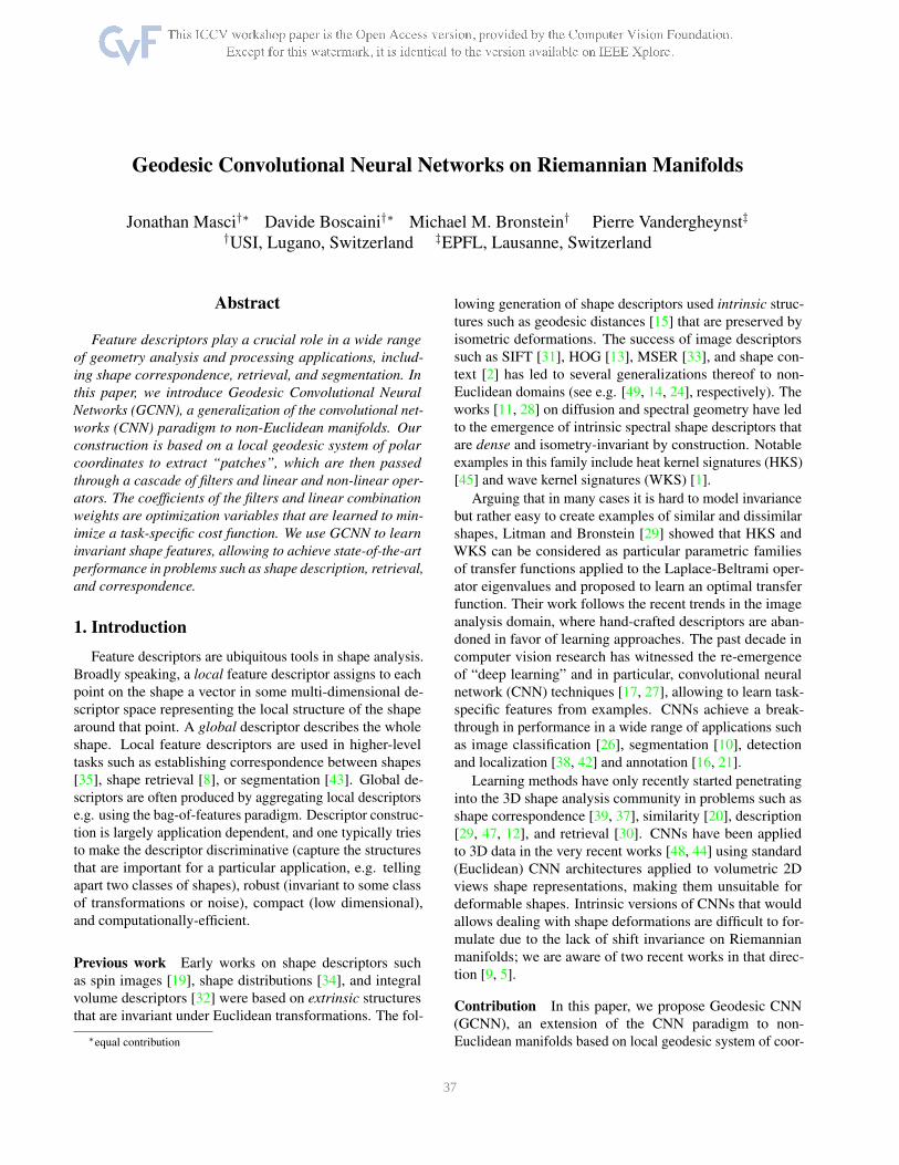
4.1. Geodesic convolution

We introduce a notion of convolution on non-Euclidean

domains that follows the ‘correlation with template’ idea by

employing a local system of geodesic polar coordinates con-

structed at point x, shown in Figure 1, to extract patches on

the manifold. The radial coordinate is constructed as -level

sets x0 : dX(x, x0) = of the geodesic (shortest path)

distance function for 2 [0, 0]; we call 0 the radius of the

geodesic disc. 1 Empirically, we see that choosing a suffi-

ciently small 0 1% of the geodesic diameter of the shape

produces valid topological discs. The angular coordinate is

constructed as a set of geodesics Γ(x, ) emanating from xin direction ; such rays are perpendicular to the geodesic

distance level sets. Note that the choice of the origin of the

angular coordinate is arbitrary. For boundary points, the pro-

cedure is very similar, with the only difference that instead

of mapping into a disc we map into a half-disc.

1 If the radius ρ0 of the geodesic ball Bρ0 (x) = x0 : dX(x, x0) ≤ρ0 is sufficiently small w.r.t the local convexity radius of the manifold,

then the resulting ball is guaranteed to be a topological disc.

vθ vρ

Figure 1: Construction of local geodesic polar coordinates

on a manifold. Left: examples of local geodesic patches,

center and right: example of angular and radial weights vθ,

vρ, respectively (red denotes larger weights).

Let Ω(x) : Bρ0(x) ! [0, 0] [0, 2) denote the bi-

jective map from the manifold into the local geodesic po-

lar coordinates (, ) around x, and let (D(x)f)(, ) =(f Ω−1(x))(, ) be the patch operator interpolating f in

the local coordinates. We can regard D(x)f as a ‘patch’ on

the manifold and use it to define what we term the geodesic

convolution (GC),

(f ? a)(x) =X

θ,r

a( +∆, r)(D(x)f)(r, ), (7)

where a(, r) is a filter applied on the patch. Due to angular

coordinate ambiguity, the filter can be rotated by arbitrary

angle ∆.

Patch operator Kokkinos et al. [24] construct the patch

operator as

(D(x)f)(, ) =

Z

X

vρ,θ(x, x0)f(x0)dx0, (8)

vρ,θ(x, x0) =

vρ(x, x0)vθ(x, x

0)R

Xvρ(x, x0)vθ(x, x0)dx0

. (9)

The radial interpolation weight is a Gaussian vρ(x, x0) /

e−(dX(x,x0)−ρ)2/σ2ρ of the geodesic distance from x, centered

around (see Figure 1, right). The angular weight is a

Gaussian vθ(x, x0) / e−d2

X(Γ(x,θ),x0)/σ2θ of the point-to-set

distance dX(Γ(x, ), x0) = minx002Γ(x,θ) dX(x00, x0) to the

geodesic Γ(x, ) (see Figure 1, center).

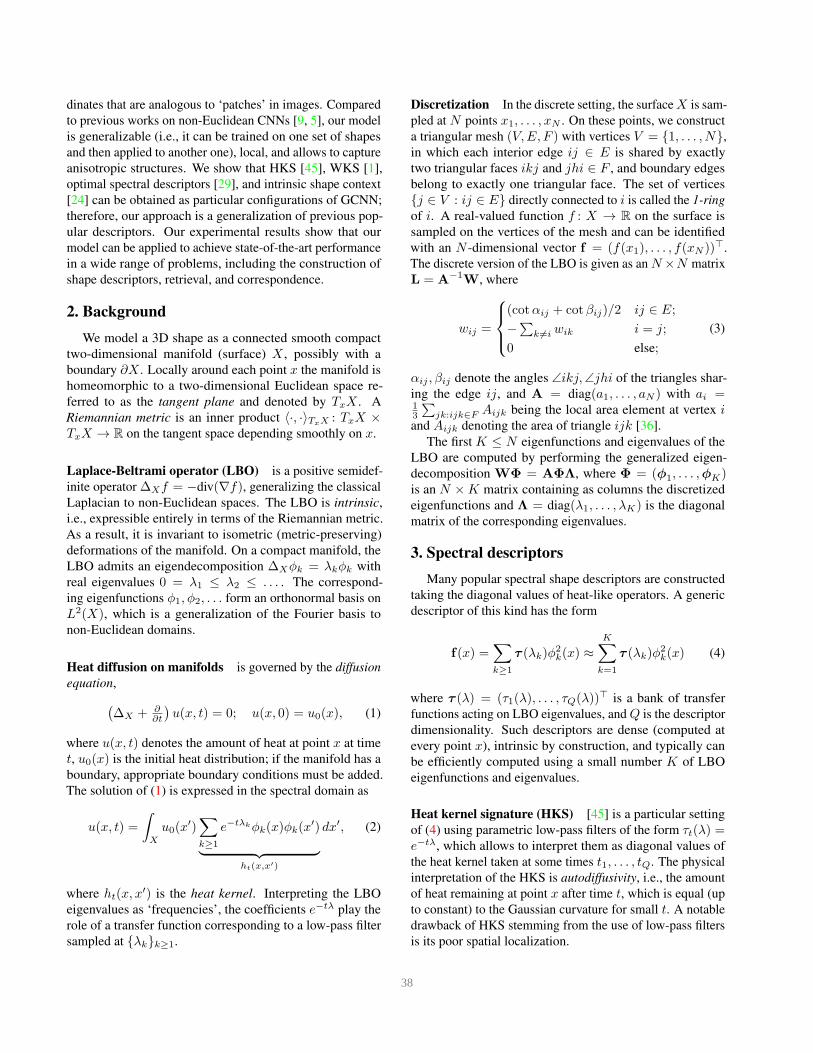
Discrete patch operator On triangular meshes, a discrete

local system of geodesic polar coordinates has Nθ angular

and Nρ radial bins. Starting with a vertex i, we first partition

the 1-ring of i by Nθ rays into equi-angular bins, aligning the

first ray with one of the edges (Figure 2). Next, we propagate

the rays into adjacent triangles using an unfolding procedure

resembling one used in [23], producing poly-lines that form

the angular bins (see Figure 2). Radial bins are created as

level sets of the geodesic distance function computed using

fast marching [23].

39

x

12

3

4

5

6 7

8

Nθ

x

θΓ(x, θ)

Figure 2: Construction of local geodesic polar coordinates

on a triangular mesh. Shown clock-wise: division of 1-ring

of vertex xi into Nθ equi-angular bins; propagation of a ray

(bold line) by unfolding the respective triangles (marked in

green).

We represent the discrete patch operator as an NθNρN N matrix applied to a function defined on the mesh vertices

and producing the patches at each vertex. The matrix is

very sparse since the values of the function at a few nearby

vertices only contribute to each local geodesic polar bin.

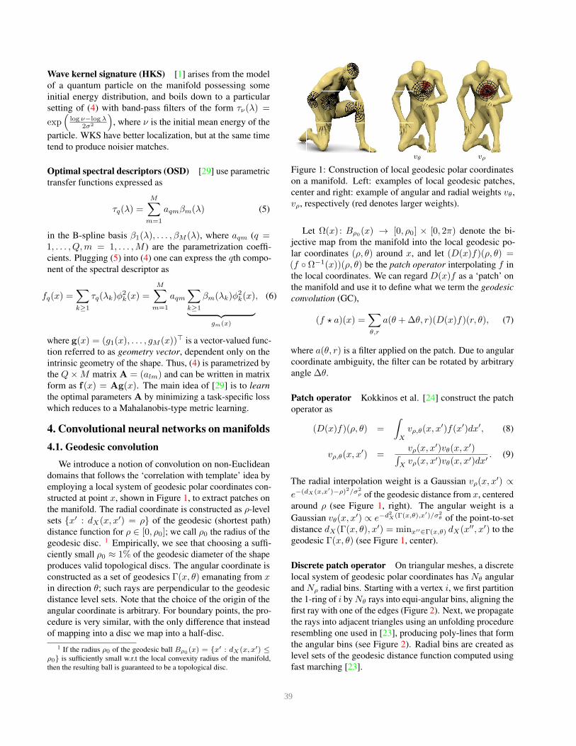
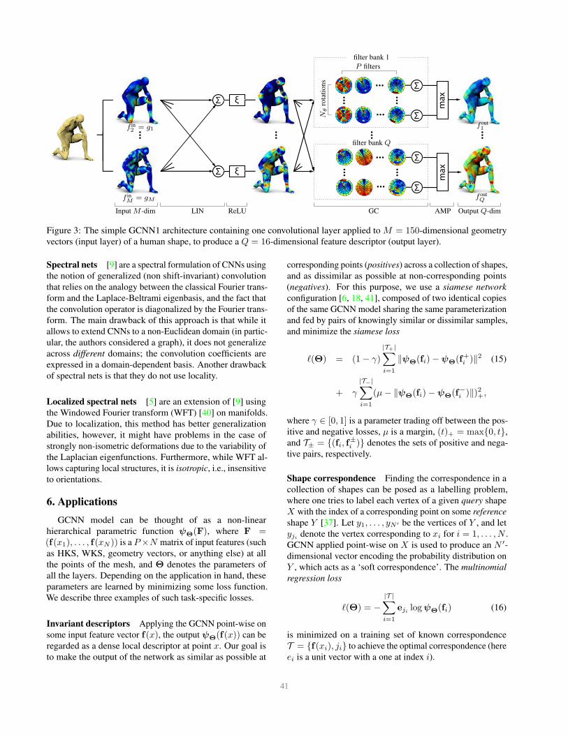
4.2. Geodesic Convolutional Neural Networks

Using the notion of geodesic convolution, we are now

ready to extend CNNs to manifolds. GCNN consists of

several layers that are applied subsequently, i.e. the output

of the previous layer is used as the input into the subsequent

one (see Figure 3). We distinguish between the following

types of layers:

Linear (LIN) layer typically follows the input layer and

precedes the output layer to adjust the input and output

dimensions by means of a linear combination,

f outq (x) =

PX

p=1

wqpfinp (x)

!

; q = 1, . . . , Q, (10)

optionally followed by a non-linear function such as the

ReLU, (t) = max0, t.

Geodesic convolution (GC) layer replaces the convolu-

tional layer used in classical Euclidean CNNs. Due to the

angular coordinate ambiguity, we compute the geodesic con-

volution result for all Nθ rotations of the filters,

fout∆θ,q(x) =

PX

p=1

(fp ? a∆θ,qp)(x), q = 1, . . . , Q, (11)

where a∆θ,qp(, r) = aqp( + ∆, r) are the coefficients

of the pth filter in the qth filter bank rotated by ∆ =

0, 2πNθ

, . . . , 2π(Nθ−1)Nθ

, and the convolution is understood in

the sense of (7).

Angular max-pooling (AMP) is a fixed layer used in con-

junction with the GC layer, that computes the maximum over

the filter rotations,

f outp (x) = max

∆θf in∆θ,p(x), p = 1, . . . , P = Q, (12)

where f in∆θ,p is the output of the GC layer (11).

Fourier transform magnitude (FTM) layer is another

fixed layer that applies the patch operator to each input di-

mension, followed by Fourier transform w.r.t. the angular

coordinate and absolute value,

f outp (,!) =

∣∣∣∣∣

X

θ

e−iωθ(D(x)f inp (x))(, )

∣∣∣∣∣, (13)

p = 1, . . . , P = Q. The Fourier transform translates rota-

tional ambiguity into complex phase ambiguity, which is

removed by taking the absolute value [25, 24].

Covariance (COV) layer is used in applications such as

retrieval where one needs to aggregate the point-wise de-

scriptors and produce a global shape descriptor [46],

f out =

Z

X

(f in(x)− µ)(f in(x)− µ)>dx, (14)

where f in(x) = (f in1 (x), . . . , f

inP (x))

> is a P -dimensional

input vector, µ =R

Xf in(x)dx, and f out is a P P matrix

column-stacked into a P 2-dimensional vector.

5. Comparison to previous approaches

Our approach is perhaps the most natural way of general-

izing CNNs to manifolds, where convolutions are performed

by sliding a window over the manifold, and local geodesic co-

ordinates are used in place of image ‘patches’. Such patches

allow capturing local anisotropic structures. Our method is

generalizable and unlike spectral approaches does not rely

on the approximate invariance of Laplacian eigenfunctions

across the shapes.

Spectral descriptors can be obtained as particular config-

urations of GCNN applied on geometry vectors input. HKS

[45] and WKS [1] descriptors are obtained by using a fixed

LIN layer configured to produce low- or band-pass filters,

respectively. OSD [29] is obtained by using a learnable

LIN layer. Intrinsic shape context [24] is obtained by us-

ing a fixed LIN layer configured to produce HKS or WKS

descriptors, followed by a fixed FTM layer.

40

...

...

...

Σ

Σ

ξ

ξ

Σ

Σ

...

...

...

...

Σ

Σ

...

...

...

...

...

max

max

Input M -dim LIN ReLU GC AMP Output Q-dim

f inM = gM

f in2

= g1

foutQ

fout1

P filters

Nθ

rota

tio

ns

filter bank 1

filter bank Q

Figure 3: The simple GCNN1 architecture containing one convolutional layer applied to M = 150-dimensional geometry

vectors (input layer) of a human shape, to produce a Q = 16-dimensional feature descriptor (output layer).

Spectral nets [9] are a spectral formulation of CNNs using

the notion of generalized (non shift-invariant) convolution

that relies on the analogy between the classical Fourier trans-

form and the Laplace-Beltrami eigenbasis, and the fact that

the convolution operator is diagonalized by the Fourier trans-

form. The main drawback of this approach is that while it

allows to extend CNNs to a non-Euclidean domain (in partic-

ular, the authors considered a graph), it does not generalize

across different domains; the convolution coefficients are

expressed in a domain-dependent basis. Another drawback

of spectral nets is that they do not use locality.

Localized spectral nets [5] are an extension of [9] using

the Windowed Fourier transform (WFT) [40] on manifolds.

Due to localization, this method has better generalization

abilities, however, it might have problems in the case of

strongly non-isometric deformations due to the variability of

the Laplacian eigenfunctions. Furthermore, while WFT al-

lows capturing local structures, it is isotropic, i.e., insensitive

to orientations.

6. Applications

GCNN model can be thought of as a non-linear

hierarchical parametric function ψΘ(F), where F =(f(x1), . . . , f(xN )) is a PN matrix of input features (such

as HKS, WKS, geometry vectors, or anything else) at all

the points of the mesh, and Θ denotes the parameters of

all the layers. Depending on the application in hand, these

parameters are learned by minimizing some loss function.

We describe three examples of such task-specific losses.

Invariant descriptors Applying the GCNN point-wise on

some input feature vector f(x), the output ψΘ(f(x)) can be

regarded as a dense local descriptor at point x. Our goal is

to make the output of the network as similar as possible at

corresponding points (positives) across a collection of shapes,

and as dissimilar as possible at non-corresponding points

(negatives). For this purpose, we use a siamese network

configuration [6, 18, 41], composed of two identical copies

of the same GCNN model sharing the same parameterization

and fed by pairs of knowingly similar or dissimilar samples,

and minimize the siamese loss

`(Θ) = (1− γ)

|T+|X

i=1

kψΘ(fi)−ψΘ(f+i )k2 (15)

+ γ

|T−|X

i=1

(µ− kψΘ(fi)−ψΘ(f−i )k)2+,

where γ 2 [0, 1] is a parameter trading off between the pos-

itive and negative losses, µ is a margin, (t)+ = max0, t,

and T± = (fi, f±i ) denotes the sets of positive and nega-

tive pairs, respectively.

Shape correspondence Finding the correspondence in a

collection of shapes can be posed as a labelling problem,

where one tries to label each vertex of a given query shape

X with the index of a corresponding point on some reference

shape Y [37]. Let y1, . . . , yN 0 be the vertices of Y , and let

yji denote the vertex corresponding to xi for i = 1, . . . , N .

GCNN applied point-wise on X is used to produce an N 0-

dimensional vector encoding the probability distribution on

Y , which acts as a ‘soft correspondence’. The multinomial

regression loss

`(Θ) = −

|T |X

i=1

eji logψΘ(fi) (16)

is minimized on a training set of known correspondence

T = f(xi), ji to achieve the optimal correspondence (here

ei is a unit vector with a one at index i).

41

Shape retrieval In the shape retrieval application, we are

interested in producing a global shape descriptor that dis-

criminates between shape classes (note that in a sense this

is the converse of invariant descriptors for correspondence,

which we wanted to be oblivious to different classes). In

order to aggregate the local features we use the COV layer

in GCNN and regard ψΘ(F) as a global shape descriptor.

Training is done by minimizing the siamese loss, where

positives and negatives are shapes from same and different

classes, respectively.

7. Results

We used the FAUST [4] dataset containing scanned hu-

man shapes in different poses and the TOSCA [7] dataset

containing synthetic models of humans in a variety of near-

isometric deformations. The meshes in TOSCA were re-

sampled to 10K vertices; FAUST shapes contained 6.8K

points. All shapes were scaled to unit geodesic diameter.

GCNN was implemented in Theano [3]. Geodesic patches

were generated using the code and settings of [24] with

0 = 1% geodesic diameter. Training was performed us-

ing the Adadelta stochastic optimization algorithm [50] for a

maximum of 2.5K updates. Typical training times on FAUST

shapes were approximately 30 and 50 minutes for one- and

two-layer models (GCNN1 and GCNN2, respectively). The

application of a trained GCNN model to compute feature

descriptors was very efficient: 75K and 45K vertices/sec for

the GCNN1 and GCNN2 models, respectively. Training and

testing was done on disjoint sets. As the input to GCNN,

we used M = 150-dimensional geometry vectors computed

according to (5)–(6) using B-spline bases. Laplace-Beltrami

operators were discretized using the cotangent formula (3);

K = 300 eigenfunctions were computed using MATLAB

eigs function.

7.1. Intrinsic shape descriptors

We first used GCNN to produce dense intrinsic pose-

and subject-invariant descriptors for human shapes, follow-

ing nearly-verbatim the experimental setup of [29]. For

reference, we compared GCNN to HKS [45], WKS [1],

and OSD [29] using the code and settings provided by

the respective authors. All the descriptors were Q = 16-

dimensional as in [29]. We used two configurations: GCNN1

(150-dim input, LIN16+ReLU, GC16+AMP shown in Fig-

ure 3), and GCNN2 (same as GCNN1 with additional ReLU,

FTM, LIN16 layers); Training of GCNN was done using the

loss (15) with positive and negative sets of vertex pairs gen-

erated on the fly. On the FAUST dataset, we used subjects

1–7 for training, subject 8 for validation, and subject 9–10for testing. On TOSCA, we test on all the deformations of

the Victoria shape.

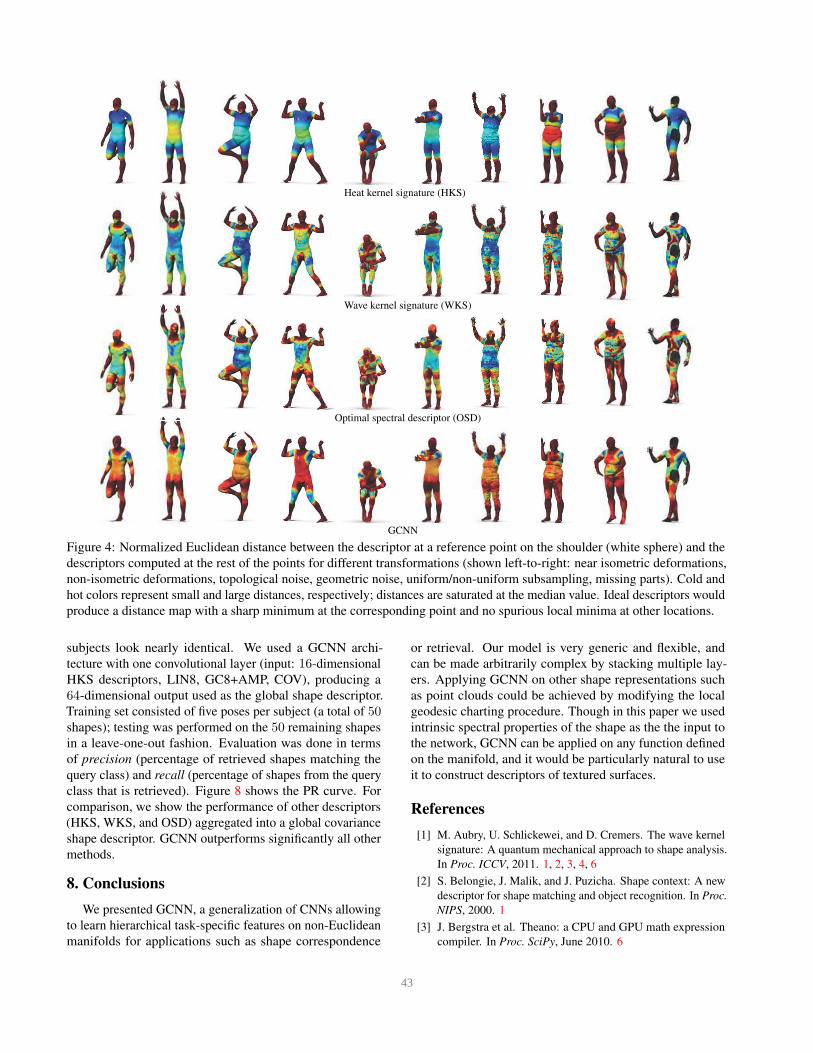
Figure 4 depicts the Euclidean distance in the descriptor

space between the descriptor at a selected point and the rest

of the points on the same shape as well as its transformations.

GCNN descriptors manifest both good localization (better

than HKS) and are more discriminative (less spurious min-

ima than WKS and OSD), as well as robustness to different

kinds of noise, including isometric and non-isometric defor-

mations, geometric and topological noise, different sampling,

and missing parts.

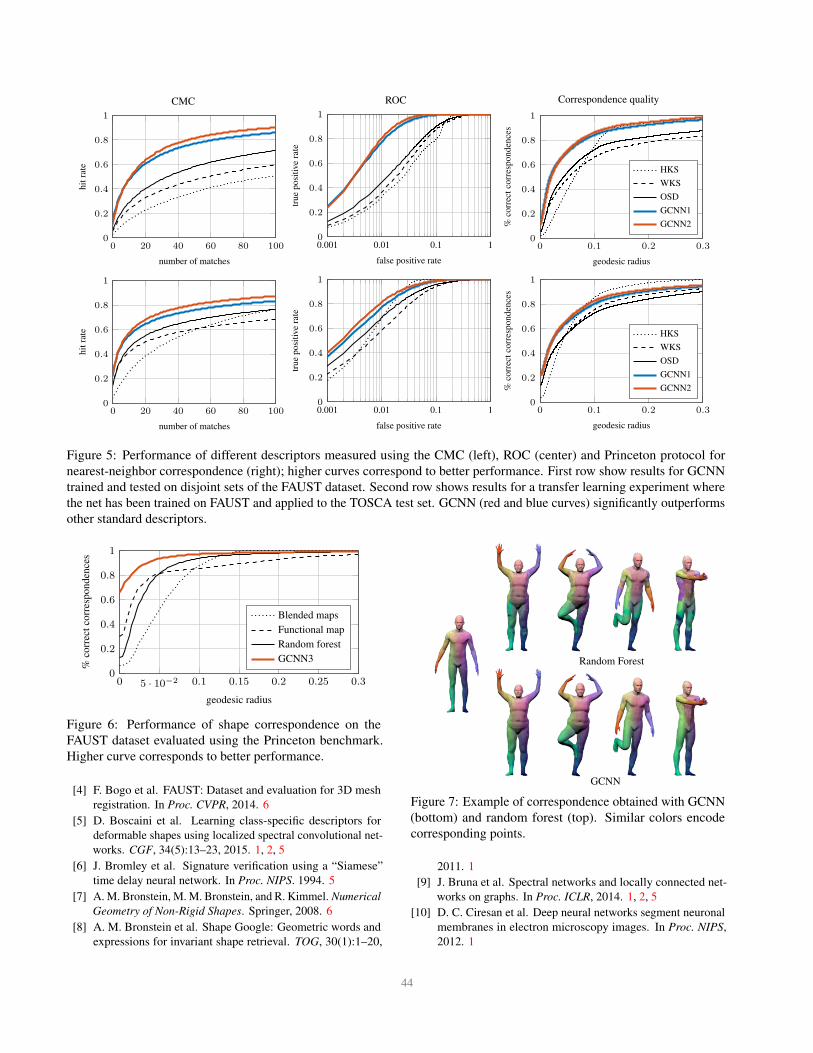
Quantitative descriptor evaluation was done using three

criteria: cumulative match characteristic (CMC), receiver

operator characteristic (ROC), and the Princeton protocol

[22]. The CMC evaluates the probability of a correct corre-

spondence among the k nearest neighbors in the descriptor

space. The ROC measures the percentage of positives and

negatives pairs falling below various thresholds of their dis-

tance in the descriptor space (true positive and negative

rates, respectively). The Princeton protocol counting the

percentage of nearest-neighbor matches that are at most r-

geodesically distant from the groundtruth correspondence.

Figure 5 (first row) shows the performance of different de-

scriptors on the FAUST dataset. We observe that GCNN

descriptors significantly outperform other descriptors, and

that the more complex model (GCNN2) further boosts per-

formance. In order to test the generalization capability of

the learned descriptors, we applied OSD and GCNN learned

on the FAUST dataset to TOSCA shapes (Figure 5, second

row). We see that the learned model transfers well to a new

dataset.

7.2. Shape correspondence

To show the application of GCNN for computing intrinsic

correspondence, we reproduced the experiment of Rodola et

al. [37] on the FAUST dataset, replacing their random forest

with a GCNN architecture GCNN3 containing three convo-

lutional layers (input: 150-dimensional geometry vectors,

LIN16+ReLU, GC32+AMP+ReLU, GC64+AMP+ReLU,

GC128+AMP+ReLU, LIN256, LIN6890). Zeroth FAUST

shape containing N 0 = 6890 vertices was used as reference;

for each point on the query shape, the output of GCNN repre-

senting the soft correspondence as an 6890-dimensional vec-

tor was converted into a point correspondence by taking the

maximum. Training was done by minimizing the loss (16);

training and test sets were as in the previous experiment.

Figure 6 shows the performance of our method evaluated

using the Princeton benchmark, and Figure 7 shows corre-

spondence examples where colors are transferred using raw

point-wise correspondence in input to the functional maps

algorithm. GCNN shows significantly better performance

than previous methods [22, 35, 37].

7.3. Shape retrieval

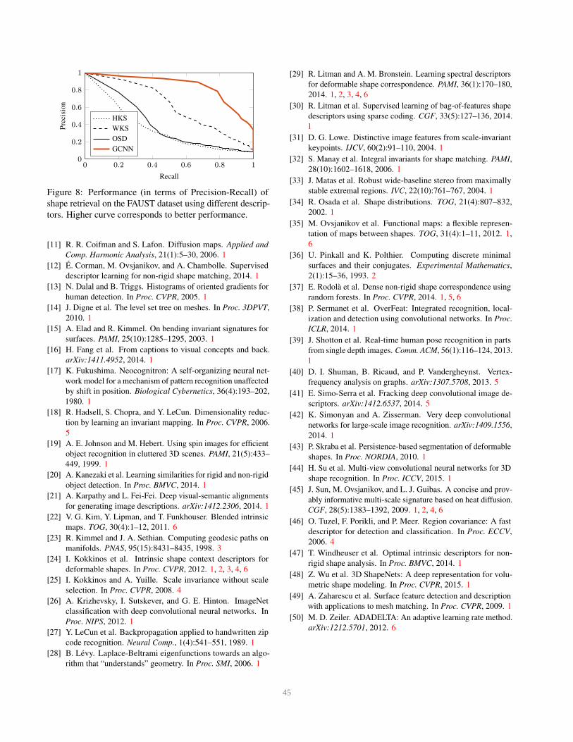
In our final experiment, we performed pose-invariant

shape retrieval on the FAUST dataset. This is a hard fine-

grained classification problem since some of the human

42

Heat kernel signature (HKS)

Wave kernel signature (WKS)

Optimal spectral descriptor (OSD)

GCNN

Figure 4: Normalized Euclidean distance between the descriptor at a reference point on the shoulder (white sphere) and the

descriptors computed at the rest of the points for different transformations (shown left-to-right: near isometric deformations,

non-isometric deformations, topological noise, geometric noise, uniform/non-uniform subsampling, missing parts). Cold and

hot colors represent small and large distances, respectively; distances are saturated at the median value. Ideal descriptors would

produce a distance map with a sharp minimum at the corresponding point and no spurious local minima at other locations.

subjects look nearly identical. We used a GCNN archi-

tecture with one convolutional layer (input: 16-dimensional

HKS descriptors, LIN8, GC8+AMP, COV), producing a

64-dimensional output used as the global shape descriptor.

Training set consisted of five poses per subject (a total of 50shapes); testing was performed on the 50 remaining shapes

in a leave-one-out fashion. Evaluation was done in terms

of precision (percentage of retrieved shapes matching the

query class) and recall (percentage of shapes from the query

class that is retrieved). Figure 8 shows the PR curve. For

comparison, we show the performance of other descriptors

(HKS, WKS, and OSD) aggregated into a global covariance

shape descriptor. GCNN outperforms significantly all other

methods.

8. Conclusions

We presented GCNN, a generalization of CNNs allowing

to learn hierarchical task-specific features on non-Euclidean

manifolds for applications such as shape correspondence

or retrieval. Our model is very generic and flexible, and

can be made arbitrarily complex by stacking multiple lay-

ers. Applying GCNN on other shape representations such

as point clouds could be achieved by modifying the local

geodesic charting procedure. Though in this paper we used

intrinsic spectral properties of the shape as the the input to

the network, GCNN can be applied on any function defined

on the manifold, and it would be particularly natural to use

it to construct descriptors of textured surfaces.

References

[1] M. Aubry, U. Schlickewei, and D. Cremers. The wave kernel

signature: A quantum mechanical approach to shape analysis.

In Proc. ICCV, 2011. 1, 2, 3, 4, 6

[2] S. Belongie, J. Malik, and J. Puzicha. Shape context: A new

descriptor for shape matching and object recognition. In Proc.

NIPS, 2000. 1

[3] J. Bergstra et al. Theano: a CPU and GPU math expression

compiler. In Proc. SciPy, June 2010. 6

43

CMC

0 20 40 60 80 1000

0.2

0.4

0.6

0.8

1

number of matches

hit

rate

ROC

0.001 0.01 0.1 10

0.2

0.4

0.6

0.8

1

false positive rate

true

posi

tive

rate

Correspondence quality

0 0.1 0.2 0.30

0.2

0.4

0.6

0.8

1

geodesic radius

%co

rrec

tco

rres

ponden

ces

HKS

WKS

OSD

GCNN1

GCNN2

0 20 40 60 80 1000

0.2

0.4

0.6

0.8

1

number of matches

hit

rate

0.001 0.01 0.1 10

0.2

0.4

0.6

0.8

1

false positive rate

true

posi

tive

rate

0 0.1 0.2 0.30

0.2

0.4

0.6

0.8

1

geodesic radius

%co

rrec

tco

rres

ponden

ces

HKS

WKS

OSD

GCNN1

GCNN2

Figure 5: Performance of different descriptors measured using the CMC (left), ROC (center) and Princeton protocol for

nearest-neighbor correspondence (right); higher curves correspond to better performance. First row show results for GCNN

trained and tested on disjoint sets of the FAUST dataset. Second row shows results for a transfer learning experiment where

the net has been trained on FAUST and applied to the TOSCA test set. GCNN (red and blue curves) significantly outperforms

other standard descriptors.

0 5 · 10−2 0.1 0.15 0.2 0.25 0.30

0.2

0.4

0.6

0.8

1

geodesic radius

%co

rrec

tco

rres

po

nd

ence

s

Blended maps

Functional map

Random forest

GCNN3

Figure 6: Performance of shape correspondence on the

FAUST dataset evaluated using the Princeton benchmark.

Higher curve corresponds to better performance.

[4] F. Bogo et al. FAUST: Dataset and evaluation for 3D mesh

registration. In Proc. CVPR, 2014. 6

[5] D. Boscaini et al. Learning class-specific descriptors for

deformable shapes using localized spectral convolutional net-

works. CGF, 34(5):13–23, 2015. 1, 2, 5

[6] J. Bromley et al. Signature verification using a “Siamese”

time delay neural network. In Proc. NIPS. 1994. 5

[7] A. M. Bronstein, M. M. Bronstein, and R. Kimmel. Numerical

Geometry of Non-Rigid Shapes. Springer, 2008. 6

[8] A. M. Bronstein et al. Shape Google: Geometric words and

expressions for invariant shape retrieval. TOG, 30(1):1–20,

Random Forest

GCNN

Figure 7: Example of correspondence obtained with GCNN

(bottom) and random forest (top). Similar colors encode

corresponding points.

2011. 1

[9] J. Bruna et al. Spectral networks and locally connected net-

works on graphs. In Proc. ICLR, 2014. 1, 2, 5

[10] D. C. Ciresan et al. Deep neural networks segment neuronal

membranes in electron microscopy images. In Proc. NIPS,

2012. 1

44

0 0.2 0.4 0.6 0.8 10

0.2

0.4

0.6

0.8

1

Recall

Pre

cisi

on

HKS

WKS

OSD

GCNN

Figure 8: Performance (in terms of Precision-Recall) of

shape retrieval on the FAUST dataset using different descrip-

tors. Higher curve corresponds to better performance.

[11] R. R. Coifman and S. Lafon. Diffusion maps. Applied and

Comp. Harmonic Analysis, 21(1):5–30, 2006. 1

[12] E. Corman, M. Ovsjanikov, and A. Chambolle. Supervised

descriptor learning for non-rigid shape matching, 2014. 1

[13] N. Dalal and B. Triggs. Histograms of oriented gradients for

human detection. In Proc. CVPR, 2005. 1

[14] J. Digne et al. The level set tree on meshes. In Proc. 3DPVT,

2010. 1

[15] A. Elad and R. Kimmel. On bending invariant signatures for

surfaces. PAMI, 25(10):1285–1295, 2003. 1

[16] H. Fang et al. From captions to visual concepts and back.

arXiv:1411.4952, 2014. 1

[17] K. Fukushima. Neocognitron: A self-organizing neural net-

work model for a mechanism of pattern recognition unaffected

by shift in position. Biological Cybernetics, 36(4):193–202,

1980. 1

[18] R. Hadsell, S. Chopra, and Y. LeCun. Dimensionality reduc-

tion by learning an invariant mapping. In Proc. CVPR, 2006.

5

[19] A. E. Johnson and M. Hebert. Using spin images for efficient

object recognition in cluttered 3D scenes. PAMI, 21(5):433–

449, 1999. 1

[20] A. Kanezaki et al. Learning similarities for rigid and non-rigid

object detection. In Proc. BMVC, 2014. 1

[21] A. Karpathy and L. Fei-Fei. Deep visual-semantic alignments

for generating image descriptions. arXiv:1412.2306, 2014. 1

[22] V. G. Kim, Y. Lipman, and T. Funkhouser. Blended intrinsic

maps. TOG, 30(4):1–12, 2011. 6

[23] R. Kimmel and J. A. Sethian. Computing geodesic paths on

manifolds. PNAS, 95(15):8431–8435, 1998. 3

[24] I. Kokkinos et al. Intrinsic shape context descriptors for

deformable shapes. In Proc. CVPR, 2012. 1, 2, 3, 4, 6

[25] I. Kokkinos and A. Yuille. Scale invariance without scale

selection. In Proc. CVPR, 2008. 4

[26] A. Krizhevsky, I. Sutskever, and G. E. Hinton. ImageNet

classification with deep convolutional neural networks. In

Proc. NIPS, 2012. 1

[27] Y. LeCun et al. Backpropagation applied to handwritten zip

code recognition. Neural Comp., 1(4):541–551, 1989. 1

[28] B. Levy. Laplace-Beltrami eigenfunctions towards an algo-

rithm that “understands” geometry. In Proc. SMI, 2006. 1

[29] R. Litman and A. M. Bronstein. Learning spectral descriptors

for deformable shape correspondence. PAMI, 36(1):170–180,

2014. 1, 2, 3, 4, 6

[30] R. Litman et al. Supervised learning of bag-of-features shape

descriptors using sparse coding. CGF, 33(5):127–136, 2014.

1

[31] D. G. Lowe. Distinctive image features from scale-invariant

keypoints. IJCV, 60(2):91–110, 2004. 1

[32] S. Manay et al. Integral invariants for shape matching. PAMI,

28(10):1602–1618, 2006. 1

[33] J. Matas et al. Robust wide-baseline stereo from maximally

stable extremal regions. IVC, 22(10):761–767, 2004. 1

[34] R. Osada et al. Shape distributions. TOG, 21(4):807–832,

2002. 1

[35] M. Ovsjanikov et al. Functional maps: a flexible represen-

tation of maps between shapes. TOG, 31(4):1–11, 2012. 1,

6

[36] U. Pinkall and K. Polthier. Computing discrete minimal

surfaces and their conjugates. Experimental Mathematics,

2(1):15–36, 1993. 2

[37] E. Rodola et al. Dense non-rigid shape correspondence using

random forests. In Proc. CVPR, 2014. 1, 5, 6

[38] P. Sermanet et al. OverFeat: Integrated recognition, local-

ization and detection using convolutional networks. In Proc.

ICLR, 2014. 1

[39] J. Shotton et al. Real-time human pose recognition in parts

from single depth images. Comm. ACM, 56(1):116–124, 2013.

1

[40] D. I. Shuman, B. Ricaud, and P. Vandergheynst. Vertex-

frequency analysis on graphs. arXiv:1307.5708, 2013. 5

[41] E. Simo-Serra et al. Fracking deep convolutional image de-

scriptors. arXiv:1412.6537, 2014. 5

[42] K. Simonyan and A. Zisserman. Very deep convolutional

networks for large-scale image recognition. arXiv:1409.1556,

2014. 1

[43] P. Skraba et al. Persistence-based segmentation of deformable

shapes. In Proc. NORDIA, 2010. 1

[44] H. Su et al. Multi-view convolutional neural networks for 3D

shape recognition. In Proc. ICCV, 2015. 1

[45] J. Sun, M. Ovsjanikov, and L. J. Guibas. A concise and prov-

ably informative multi-scale signature based on heat diffusion.

CGF, 28(5):1383–1392, 2009. 1, 2, 4, 6

[46] O. Tuzel, F. Porikli, and P. Meer. Region covariance: A fast

descriptor for detection and classification. In Proc. ECCV,

2006. 4

[47] T. Windheuser et al. Optimal intrinsic descriptors for non-

rigid shape analysis. In Proc. BMVC, 2014. 1

[48] Z. Wu et al. 3D ShapeNets: A deep representation for volu-

metric shape modeling. In Proc. CVPR, 2015. 1

[49] A. Zaharescu et al. Surface feature detection and description

with applications to mesh matching. In Proc. CVPR, 2009. 1

[50] M. D. Zeiler. ADADELTA: An adaptive learning rate method.

arXiv:1212.5701, 2012. 6

45