Geodesic Object Proposals

Philipp Krahenbuhl1 and Vladlen Koltun2

1 Stanford University2 Adobe Research

Abstract. We present an approach for identifying a set of candidateobjects in a given image. This set of candidates can be used for objectrecognition, segmentation, and other object-based image parsing tasks.To generate the proposals, we identify critical level sets in geodesic dis-tance transforms computed for seeds placed in the image. The seedsare placed by specially trained classifiers that are optimized to discoverobjects. Experiments demonstrate that the presented approach achievessignificantly higher accuracy than alternative approaches, at a fractionof the computational cost.

Keywords: perceptual organization, grouping

1 Introduction

Many image parsing pipelines use sliding windows to extract densely overlappingbounding boxes that are then analyzed [7,11,22]. This approach has well-knowndisadvantages: the number of bounding boxes per image must be very large toachieve good recognition accuracy, most of the computational effort is wasted onfutile bounding boxes, and the rectangular boxes aggregate visual informationfrom multiple objects and background clutter. Both recognition accuracy andcomputational performance suffer as a result.

An alternative approach is to use segmentation to extract a set of proposedobjects to be analyzed [5,9,12,15,21]. Ideal object proposals of this kind shouldencapsulate the visual signal from one object and have informative boundaryshape cues that can assist subsequent tasks. Image analysis pipelines based onsuch segmentation-driven object proposals have recently achieved state-of-the-art performance on challenging benchmarks [3,4].

In this paper, we present an approach that produces highly accurate objectproposals with minimal computational overhead per image. Our key idea is toidentify critical level sets in geodesic distance transforms computed for judi-ciously placed seeds in the image. The seeds are placed by classifiers that aretrained to discover objects. Since the geodesic distance transform can be com-puted in near-linear time and since each computed transform is used to generateproposals at different scales, the pipeline is extremely efficient.

Our experiments demonstrate that the presented approach achieves signifi-cantly higher accuracy than alternative approaches as measured by both bound-ing box overlap and detailed shape overlap with ground-truth objects. It is alsosubstantially faster, producing a high-performing set of object proposals for araw input image in less than a second using a single CPU thread.

2 Philipp Krahenbuhl, Vladlen Koltun

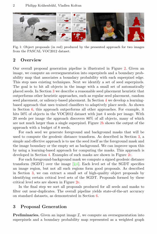
Fig. 1: Object proposals (in red) produced by the presented approach for two imagesfrom the PASCAL VOC2012 dataset.

2 Overview

Our overall proposal generation pipeline is illustrated in Figure 2. Given animage, we compute an oversegmentation into superpixels and a boundary prob-ability map that associates a boundary probability with each superpixel edge.This step uses existing techniques. Next we identify a set of seed superpixels.The goal is to hit all objects in the image with a small set of automaticallyplaced seeds. In Section 3 we describe a reasonable seed placement heuristic thatoutperforms other heuristic approaches, such as regular seed placement, randomseed placement, or saliency-based placement. In Section 4 we develop a learning-based approach that uses trained classifiers to adaptively place seeds. As shownin Section 6, this approach outperforms all other approaches. For example, ithits 50% of objects in the VOC2012 dataset with just 4 seeds per image. With20 seeds per image the approach discovers 80% of all objects, many of whichare not much larger than a single superpixel. Figure 2b shows the output of theapproach with a budget of 8 seeds.

For each seed we generate foreground and background masks that will beused to compute the geodesic distance transform. As described in Section 3, asimple and effective approach is to use the seed itself as the foreground mask andthe image boundary or the empty set as background. We can improve upon thisby using a learning-based approach for computing the masks. This approach isdeveloped in Section 4. Examples of such masks are shown in Figure 2c.

For each foreground-background mask we compute a signed geodesic distancetransform (SGDT) over the image [2,6]. Each level set of the SGDT specifiesan image region, but not all such regions form good proposals. As describedin Section 3, we can extract a small set of high-quality object proposals byidentifying certain critical level sets of the SGDT. Proposals formed by thesecritical level sets are shown in Figure 2e.

In the final step we sort all proposals produced for all seeds and masks tofilter out near-duplicates. The overall pipeline yields state-of-the-art accuracyon standard datasets, as demonstrated in Section 6.

3 Proposal Generation

Preliminaries. Given an input image I, we compute an oversegmentation intosuperpixels and a boundary probability map represented as a weighted graph

Geodesic Object Proposals 3

(a) Input (b) Seeds (c) Masks (d) SGDT (e) Proposals

Fig. 2: Overall proposal generation pipeline. (a) Input image with a computed super-pixel segmentation and a boundary probability map. (b) Seeds placed by the presentedapproach. (c) Foreground and background masks generated by the presented approachfor two of these seeds. (d) Signed geodesic distance transforms for these masks. (e)Object proposals, computed by identifying critical level sets in each SGDT.

GI = (VI , EI). This is done using existing techniques, as described in Section 5.Each node x ∈ VI corresponds to a superpixel, each edge (x, y) ∈ EI connectsadjacent superpixels, and the edge weight w(x, y) represents the likelihood ofobject boundary at the corresponding image edge.

The geodesic distance dx,y between two nodes x, y ∈ VI is the length of theshortest path between the nodes in GI . The geodesic distance transform (GDT)measures the geodesic distance from a set of nodes Y ⊂ VI to each node x ∈ VI :

D(x;Y ) = miny∈Y

dx,y. (1)

The GDT for all nodes in VI can be computed exactly using Dijkstra’s algorithmin total time O(n log n), where n is the number of superpixels. Linear-time ap-proximations exist for regular grids [20,23], but our domain is not regular andwe use the exact solution.

The geodesic distance transform can be generalized to consider a foregroundset F ⊂ VI and a background set B ⊂ VI [2,6]. In this case, the signed geodesicdistance transform (SGDT) is defined as

D(x;F,B) = D(x;F )−D(x;B). (2)

Each level set λ of the SGDT encloses a unique image segment, which can beused as an object proposal:

Pλ = {x : D(x;F,B) < λ} . (3)

Our approach consists of computing promising foreground and background setsand identifying a small set of appropriate level sets λ for each foreground-background pair. The rest of this section describes the different stages of theapproach. We begin by computing a set of foreground seeds: individual super-pixels that are likely to be located inside objects. For each such seed, we constructforeground and background masks. For each pair of masks, we identify a smallset of level sets. Each level set specifies an object proposal.

4 Philipp Krahenbuhl, Vladlen Koltun

Seed placement. Our first task is to identify a small set of seed nodes S ⊂ VI .The goal is to hit all the objects in the image with a small number of seeds, soas to minimize the overall number of object proposals that must be processed bythe recognition pipeline. As shown in Section 6, naive seed selection strategies donot perform well. Both regular sampling and random sampling fail to discoversmall objects in images unless an exorbitant number of seeds is used. Saliency-based seed placement also performs poorly since it is not effective at identifyingless prominent objects. We now describe a better seed selection heuristic, basedon greedy minimization of geodesic distances.

The heuristic proceeds iteratively. The first seed is placed in the geodesiccenter of the image:

S ← {arg mins

maxy∈VI

ds,y}. (4)

The geodesic center is the superpixel for which the maximal geodesic distance toall other superpixels is minimized. It lies halfway on the longest geodesic pathin the superpixel graph and can be found using three consecutive shortest pathcomputations.

Each of the following seeds is placed so as to maximize its geodesic distanceto previous seeds:

S ← S ∪ {arg maxs

D(s;S)}. (5)

This is repeated until the desired number of seeds is reached. The arg max inEquation 5 can be evaluated with one execution of Dijkstra’s algorithm on GI ,thus the total runtime of the algorithm is O(NSn log n), where NS is the numberof seeds. The algorithm can be interpreted as greedy minimization of the maximalgeodesic distance of all superpixels to the seed set.

This algorithm considerably outperforms the naive approaches. It will inturn be superseded in Section 4 by a learning-based approach, but it is a simpleheuristic that performs well and may be sufficient for some applications.

Foreground and background masks. For each seed s ∈ S, we generate fore-ground and background masks Fs, Bs ⊂ VI that are used as input to the SGDT.The goal here is to focus the SGDT on object boundaries by possibly expandingthe foreground mask to include more of the interior of the object that containsit, as well as masking out parts of the image that are likely to be outside theobject. This is a challenging task because at this stage we don’t know what theobject is: it may be as small as a single superpixel or so large as to span mostof the image. We will tackle this problem systematically in Section 4, where alearning-based approach to generate foreground and background masks will bedeveloped. As a baseline we will use the seed itself as the foreground mask. Forthe background we will use two masks: an empty one and the image boundary.

Critical level sets. Given a foreground-background mask, our goal is to com-pute a small set of intermediate level sets that delineate the boundaries of objectsthat include the foreground. Prior work on interactive geodesic segmentation con-sidered a single segmentation specified by the zero level set of the SGDT [2,6,19].

Geodesic Object Proposals 5

(a) Image and masks (b) SGDT

0.4 0.2 0.0 0.2 0.4 0.60

200

400

600

800

1000

(c) Critical level sets (d) Proposals

Fig. 3: (a) An image with a foreground mask (red) and a background mask (blue). (b)The corresponding signed geodesic distance transform. (c) Critical level sets identifiedby our algorithm. (d) Corresponding object proposals.

However, the zero level set is sensitive to the detailed form of the masks and maynot adhere to object boundaries [18]. We perform a more detailed analysis thatyields a small number of level sets that capture object boundaries much betterin the absence of interactive refinement by a human user.

Our analysis is based on the growth of the region Pλ as a function of λ. Specif-ically, let A(λ) = |Pλ| be the area enclosed by Pλ. This function is illustratedin Figure 3c. Observe that when the λ level set reaches an object boundary, theevolution of the level set slows down. On the other hand, when the level setpropagates through an object interior, it evolves rapidly. We can thus identifylevel sets that follow object boundaries by analyzing their evolution rate, givenby the derivative dA

dλ . Specifically, to extract object proposals that adhere to

object boundaries, we identify strong local minima of dAdλ .

Selecting level sets purely by their evolution rate can lead to a lopsidedselection, in which most proposals specify almost identical regions. To ensurediversity in the level set selection, we enforce the additional constraint that notwo selected proposals can overlap by a factor of more than α. Overlap is defined

as the Jaccard coefficient of two regions: J (Pλi ,Pλj ) =|Pλi ||Pλj |

for λi < λj . (Note

that λi < λj implies Pλi ⊆ Pλj .) We greedily select the critical level sets byiteratively choosing non-overlapping proposals with the lowest evolution rate.We stop when the desired number of proposals is reached or when no morenon-overlapping level sets remain.

Once all proposals from all seeds are generated, we sort them by their evo-lution rate, which serves as a proxy for their quality. We then greedily selectproposals that overlap with prior selections by at most α. To efficiently checkthe overlap between two proposals we use a hierarchical spatial data structure.

4 Learning Seed Placement and Mask Construction

The proposal generation pipeline described in Section 3 performs very well, asshown in Section 6. However, we can enhance its performance further by replac-ing two heuristic steps in the pipeline with learning-based approaches. Thesetwo steps are the seed placement algorithm and the construction of foregroundand background masks.

6 Philipp Krahenbuhl, Vladlen Koltun

Learning to place seeds. We now develop a learning-based approach for seedplacement. The approach places seeds sequentially. We train a linear rankingclassifier for the placement of each seed si, for i = 1, . . . , NS . This allows theplacement strategy to adapt: the objective that is optimized by the placement ofthe first seeds need not be the same as the objective optimized by the placementof later seeds. For example, early seeds can prioritize hitting large and prominentobjects in the image, while later seeds can optimize for discovering a variety ofsmaller objects that may require specialized objectives.

At each iteration i, we compute features f(i)x for each possible seed location

x ∈ VI . These features include static features such as location within the imageand adaptive features such as distance to previously placed seeds. In general,

the feature values are a function of previously placed seeds: f(i)x 6= f

(j)x for i 6= j.

The specific features we use are listed in Section 5.The classifier for iteration i is trained after classifiers for iterations j < i.

For iteration i, we train a linear ranking classifier that associates a score w>i f

with any feature vector f . During inference we place seed si in the top ranking

location as determined by the trained classifier: si = arg maxxw>i f

(i)x . The train-

ing optimizes the weight vector wi. For the training, we partition each trainingimage I into a positive region PI and a negative region NI . The positive regionconsists of all superpixels contained in ground truth objects in the image thathave not been hit by previously placed seeds. (The seeds are placed by classifierspreviously trained for iterations j < i.) The negative region is simply the com-plement of the positive region: NI = VI \ PI . We will now formulate a learningobjective that encourages the placement of seed si inside the positive region PIin as many images I as possible.

Our learning objective differs substantially from standard ranking methods[13]. Standard algorithms aim to learn a ranking that fits a given complete or par-tial ordering on the data. In our setting, such a partial ordering can be obtained

by ranking feature vectors associated with each positive region (f(i)x for x ∈ PI)

above feature vectors associated with the corresponding negative region NI .While this standard objective works well for early seeds, it ceases to be effectivein later iterations when no parameter setting wi can reasonably separate thepositive region from the negative.

Our key insight is that we do not need to rank all positive seed locations aboveall negative ones. Our setting only demands that the highest-ranking location bein the positive set, since we only place one seed si at iteration i. This objectivecan be formalized as finding a weight vector wi that ranks the highest-rankingpositive seed x ∈ PI above the highest-ranking negative seed y ∈ NI . We use

logistic regression on the difference between the two scores: w>i f

(i)x − w>

i f(i)y .

The log-likelihood of the logistic regression is given by

`I(wi) = log

(1 + exp

(maxx∈NI

w>i f

(i)x − max

x∈PIw>i f

(i)x

)). (6)

This objective is both non-convex and non-smooth, which makes it impossibleto compute gradients or subgradients. However, we can replace each maximum

Geodesic Object Proposals 7

maxxw>i f

(i)x in Equation 6 with the softmax log

∑x exp(w>

i f(i)x ), which can be

used to simplify the objective to

`I(wi) = log∑x∈VI

exp(w>i f

(i)x

)− log

∑x∈PI

exp(w>i f

(i)x

). (7)

This objective is smooth and any gradient-based optimization algorithm such asL-BFGS can be used to minimize it. While the second term in the objective isstill non-convex, the optimization is very robust in practice. In our experiments,a wide variety of different initializations yield the same local minimum.

Learning to construct masks. Given a seed s ∈ S, we generate foregroundand background masks Fs, Bs ⊂ VI . These masks give us a chance to furtherdirect the geodesic segmentation to object boundaries by labeling some imageregions as foreground or background. Given the formulation of the SGDT, thesemasks must be conservative: the foreground mask must be contained inside thesought object and the background mask must be outside.

To construct masks, we train one linear classifier for the foreground maskand one linear classifier for the background mask. Both classifiers operate on

features f(s)x , where s is the given seed and x ∈ VI is a superpixel in the image.

The training optimizes a weight vector wF for the foreground classifier and aweight vector wB for the background classifier.

We begin by considering the learning objective for the foreground classi-fier. This objective should reward the generation of the largest foreground maskFs ⊆ Os, where Os is the ground-truth object that encloses seed s. The contain-ment in Os is a hard constraint: the foreground mask should not leak outsidethe object boundary. This can be formalized as follows:

minimizewF

∑s

∑x∈Os

ρ(w>F f

(s)x

)subject to ∀s ∈ S ∀y /∈ Os w>

F f(s)y < 0.

(8)

Here ρ is a penalty function that maximizes the number of true positives. Weuse the hinge loss, which allows us to minimize Equation 8 as a standard linearSVM with a high negative class weight.

The hard constraints in Equation 8 need to be satisfied for a large numberof training objects Os with hugely varying appearance and size. In our initialexperiments, simply optimizing this objective led to trivial classifiers that sim-ply produce the initial seed as the foreground mask and the empty set for thebackground mask. (The learning objective for the background mask is analogousto Equation 8.) To overcome this difficulty, we modify the formulation to trainseveral classifiers. At inference time, we simply use each of the trained classifiersto generate object proposals. The basic idea is that one of the learned classifiersabsorbs the challenging training examples that demand a highly conservativeresponse (trivial foreground and background masks), while others can handleexamples that allow larger masks.

8 Philipp Krahenbuhl, Vladlen Koltun

(a) Image (b) Mask 1 (c) Mask 2 (d) Mask 3

Fig. 4: The output of learned mask classifiers. (a) Input image. (b-d) Foreground andbackground masks generated for a given seed by the learned classifiers. The first clas-sifier is maximally conservative, the others are more risk-taking.

Specifically, we train K foreground classifiers, with weight vectors w(k)F for

k = 1, . . . ,K. (We use K = 3.) In addition to the weight vectors, we alsooptimize a label ks for each seed s. This is a latent variable ks ∈ {1, . . . ,K} thatassociates each training seed s with one of the classifiers. The classifiers and theassociations are optimized in concert using the following objective:

minimizew

(k)F ,ks

∑s

∑x∈Os

ρ(w

(ks)F · f (s)x

)subject to ∀s ∈ S ∀y /∈ Os w

(ks)F · f (s)y < 0.

(9)

We use alternating optimization. The different classifiers w(k)F are initialized by

picking K random seeds and optimizing the objective in Equation 8 for each ofthese seeds separately. We next optimize the associations ks by evaluating eachclassifier on each seed s and associating each seed with the classifier that yieldsthe lowest objective value on that seed. We then alternate between optimizingthe classifier parameters given fixed associations and optimizing the associationsgiven fixed classifiers. Note that each step decreases the compound objective inEquation 9.

The extension of the objective and the algorithm to incorporate backgroundmask classifiers is straightforward. In the complete formulation, we train K pairs

(w(k)F ,w

(k)B ) of foreground and background classifiers. For each seed, the label

ks associates it with both the foreground classifier w(ks)F and the background

classifier w(ks)B .

Figure 4 demonstrates the output of the learned mask classifiers on an ex-ample test seed. As expected, one of the classifiers is conservative, using theinput seed as the foreground and the empty set as the background. The otherclassifiers are more risk-taking. At test time we use all K masks for each seed togenerate object proposals.

5 Implementation

We compute a boundary probability image using structured forests [8]. Thisboundary probability image is used to produce a superpixel segmentation. Weuse the geodesic k-means algorithm, which produces a regular oversegmentation

Geodesic Object Proposals 9

that adheres to strong boundaries [17]. Both algorithms are extremely efficient,with a combined runtime of 0.5 seconds for images of size 350× 500.

Seed features used by the classifiers described in Section 4 include imagecoordinates x and y, normalized to the interval [−1, 1], as well as absolute andsquared normalized coordinates. We further use the minimal color and spatialdistance to previously placed seeds, as well as the color covariance between thegiven superpixel pixels and all seed pixels. We also add geodesic distances topreviously placed seeds, as well as to the image boundary. For computing thesedistances, we use both graphs with constant edge weights and with boundaryprobability weights.

Mask features used by the classifiers described in Section 4 include loca-tion relative to the seed, distance to each of the image boundary edges, andcolor similarity to the seed in both RGB and Lab color space. We also computecolor histograms for each superpixel and use the χ2 distance between the colorhistogram of the given superpixel and the seed superpixel. Finally we add anindicator feature for the seed itself, which ensures that there always exists aparameter setting satisfying Equation 9.

6 Evaluation

We evaluate the presented approach on the PASCAL VOC2012 dataset [10]. Allsegmentation experiments are performed on the 1449 validation images of theVOC2012 segmentation dataset. Bounding box experiments are performed onthe larger detection dataset with 5823 annotated validation images. We train allclassifiers on the 1464 segmentation training images. Training all seed and maskclassifiers takes roughly 10 minutes in total. All experiments were performed ona 3.4 GHz Core i7 processor. Runtimes for all methods are reported for single-threaded execution and cover all operations, including boundary detection andoversegmentation.

To evaluate the quality of our object proposals we use the Average BestOverlap (ABO), covering, and recall measures [5]. The ABO between a groundtruth object set S and a set of proposals P is computed using the overlap betweeneach ground truth region R ∈ S and the closest object proposal R′ ∈ P:

ABO =1

|S|∑R∈S

maxR′∈P

J (R,R′).

Here the overlap of two image regions R and R′ is defined as their Jaccard

coefficient J (R,R′) = |R∩R′||R∪R′| . Figure 5 illustrates the relationship between the

precision of fit of the two image regions and the corresponding Jaccard coefficientvalues.

Covering is an area-weighted measure:

Covering =1∑

R∈S |R|∑R∈S|R| max

R′∈PJ (R,R′).

10 Philipp Krahenbuhl, Vladlen Koltun

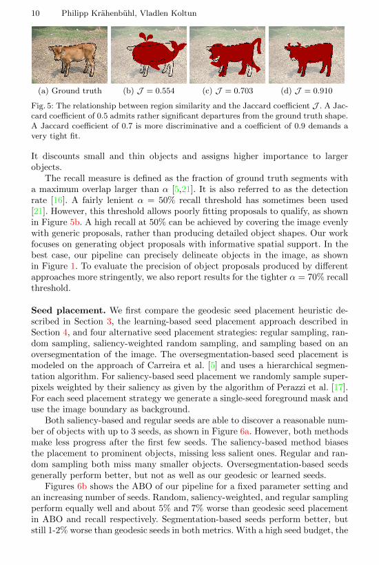
(a) Ground truth (b) J = 0.554 (c) J = 0.703 (d) J = 0.910

Fig. 5: The relationship between region similarity and the Jaccard coefficient J . A Jac-card coefficient of 0.5 admits rather significant departures from the ground truth shape.A Jaccard coefficient of 0.7 is more discriminative and a coefficient of 0.9 demands avery tight fit.

It discounts small and thin objects and assigns higher importance to largerobjects.

The recall measure is defined as the fraction of ground truth segments witha maximum overlap larger than α [5,21]. It is also referred to as the detectionrate [16]. A fairly lenient α = 50% recall threshold has sometimes been used[21]. However, this threshold allows poorly fitting proposals to qualify, as shownin Figure 5b. A high recall at 50% can be achieved by covering the image evenlywith generic proposals, rather than producing detailed object shapes. Our workfocuses on generating object proposals with informative spatial support. In thebest case, our pipeline can precisely delineate objects in the image, as shownin Figure 1. To evaluate the precision of object proposals produced by differentapproaches more stringently, we also report results for the tighter α = 70% recallthreshold.

Seed placement. We first compare the geodesic seed placement heuristic de-scribed in Section 3, the learning-based seed placement approach described inSection 4, and four alternative seed placement strategies: regular sampling, ran-dom sampling, saliency-weighted random sampling, and sampling based on anoversegmentation of the image. The oversegmentation-based seed placement ismodeled on the approach of Carreira et al. [5] and uses a hierarchical segmen-tation algorithm. For saliency-based seed placement we randomly sample super-pixels weighted by their saliency as given by the algorithm of Perazzi et al. [17].For each seed placement strategy we generate a single-seed foreground mask anduse the image boundary as background.

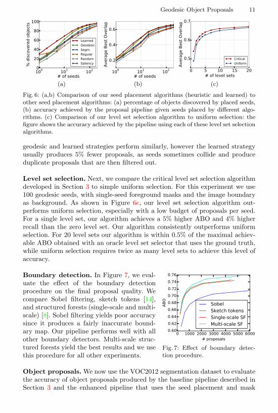
Both saliency-based and regular seeds are able to discover a reasonable num-ber of objects with up to 3 seeds, as shown in Figure 6a. However, both methodsmake less progress after the first few seeds. The saliency-based method biasesthe placement to prominent objects, missing less salient ones. Regular and ran-dom sampling both miss many smaller objects. Oversegmentation-based seedsgenerally perform better, but not as well as our geodesic or learned seeds.

Figures 6b shows the ABO of our pipeline for a fixed parameter setting andan increasing number of seeds. Random, saliency-weighted, and regular samplingperform equally well and about 5% and 7% worse than geodesic seed placementin ABO and recall respectively. Segmentation-based seeds perform better, butstill 1-2% worse than geodesic seeds in both metrics. With a high seed budget, the

Geodesic Object Proposals 11

100 101 102

# of seeds

0

20

40

60

80

100%

dis

cove

red

obje

cts

LearnedGeodesicSegm.RegularRandomSaliency

(a)

100 101 102

# of seeds

0.2

0.4

0.6

Aver

age

Best

Ove

rlap

(b)

0 5 10 15 20# of level sets

0.5

0.6

0.7

Avera

ge B

est

Overl

ap

Critical

Uniform

(c)

Fig. 6: (a,b) Comparison of our seed placement algorithms (heuristic and learned) toother seed placement algorithms: (a) percentage of objects discovered by placed seeds,(b) accuracy achieved by the proposal pipeline given seeds placed by different algo-rithms. (c) Comparison of our level set selection algorithm to uniform selection: thefigure shows the accuracy achieved by the pipeline using each of these level set selectionalgorithms.

geodesic and learned strategies perform similarly, however the learned strategyusually produces 5% fewer proposals, as seeds sometimes collide and produceduplicate proposals that are then filtered out.

Level set selection. Next, we compare the critical level set selection algorithmdeveloped in Section 3 to simple uniform selection. For this experiment we use100 geodesic seeds, with single-seed foreground masks and the image boundaryas background. As shown in Figure 6c, our level set selection algorithm out-performs uniform selection, especially with a low budget of proposals per seed.For a single level set, our algorithm achieves a 5% higher ABO and 4% higherrecall than the zero level set. Our algorithm consistently outperforms uniformselection. For 20 level sets our algorithm is within 0.5% of the maximal achiev-able ABO obtained with an oracle level set selector that uses the ground truth,while uniform selection requires twice as many level sets to achieve this level ofaccuracy.

0 1000 2000 3000 4000 5000 6000# proposals

0.60

0.62

0.64

0.66

0.68

0.70

0.72

0.74

0.76

AB

O

SobelSketch tokensSingle-scale SFMulti-scale SF

Fig. 7: Effect of boundary detec-tion procedure.

Boundary detection. In Figure 7, we eval-uate the effect of the boundary detectionprocedure on the final proposal quality. Wecompare Sobel filtering, sketch tokens [14],and structured forests (single-scale and multi-scale) [8]. Sobel filtering yields poor accuracysince it produces a fairly inaccurate bound-ary map. Our pipeline performs well with allother boundary detectors. Multi-scale struc-tured forests yield the best results and we usethis procedure for all other experiments.

Object proposals. We now use the VOC2012 segmentation dataset to evaluatethe accuracy of object proposals produced by the baseline pipeline described inSection 3 and the enhanced pipeline that uses the seed placement and mask

12 Philipp Krahenbuhl, Vladlen Koltun

Method # prop. ABO Covering 50%-recall 70%-recall Time

CPMC [5] 646 0.703 0.850 0.784 0.609 252sCat-Ind OP [9] 1536 0.718 0.840 0.820 0.624 119sSelective Search [21] 4374 0.735 0.786 0.891 0.597 2.6s

Baseline GOP (130,5) 653 0.712 0.812 0.833 0.622 0.6sBaseline GOP (150,7) 1090 0.727 0.828 0.847 0.644 0.65sBaseline GOP (200,10) 2089 0.744 0.843 0.867 0.673 0.9sBaseline GOP (300,15) 3958 0.756 0.849 0.881 0.699 1.2s

Learned GOP (140,4) 652 0.720 0.815 0.844 0.632 1.0sLearned GOP (160,6) 1199 0.741 0.835 0.865 0.673 1.1sLearned GOP (180,9) 2286 0.756 0.852 0.877 0.699 1.4sLearned GOP (200,15) 4186 0.766 0.858 0.889 0.715 1.7s

Table 1: Accuracy and running time for three state-of-the-art object proposal methodscompared to accuracy and running time for our approach. Results are provided for ourbaseline pipeline (Baseline GOP) and the enhanced pipeline that uses seed placementand mask construction classifiers (Learned GOP). Different budgets (NS ,NΛ) for seedplacement and level set selection control the number of generated proposals (# prop).

construction classifiers described in Section 4. Table 1 compares the accuracyof our pipeline (GOP) to three state-of-the-art object proposal methods, eachof which produces a different number of segments. We set the number of seedsNS and number of level sets NΛ in our pipeline to different values to roughlymatch the number of proposals produced by the other approaches. Accuracy isevaluated using ABO, covering, and recall at J ≥ 50% and J ≥ 70%.

100 101 102 103 104 105 106

size (#pixels)

0.0

0.2

0.4

0.6

0.8

1.0

best

overl

ap

GOPCPMC

Fig. 8: Accuracy of CMPC andGOP as a function of segment size.

Our baseline performs slightly better thanCPMC [5] in ABO and 70%-recall and greatlyoutperforms it at 50%-recall. CPMC is bet-ter at proposing larger objects, which leadsto higher covering results. Figure 8 provides amore detailed comparison. CPMC is based ongraph cuts and is less sensitive to texture vari-ations within large objects. However, CPMCis more than two orders of magnitude slowerthan GOP, making it impractical for largerdatasets. Evaluating CPMC on 1464 imagestook two full days on an 8-core processor,while GOP processed the dataset in less than two minutes on the same ma-chine. (0.6 seconds per image on a single core.)

Baseline GOP outperforms category-independent object proposals [9] usingjust two-thirds of the number of proposals. Again our approach is two orders ofmagnitude faster.

Selective search [21] performs extremely well at 50%-recall. However, whenthe recall threshold is increased to 70% our approach significantly outperformsselective search. At this threshold, Baseline GOP with 660 proposals outperformsthe recall achieved by selective search with more than 4000 proposals. When the

Geodesic Object Proposals 13

101 102 103

# of boxes

0.0

0.2

0.4Re

call

GOPObjectnessRandomized PrimSelective Search

(a) J ≥ 0.9

101 102 103

# of boxes

0.0

0.2

0.4

0.6

0.8

Reca

ll

(b) J ≥ 0.7

101 102 103

# of boxes

0.0

0.2

0.4

0.6

0.8

1.0

Reca

ll

(c) J ≥ 0.5

0.5 0.6 0.7 0.8 0.9 1.0J

0.0

0.2

0.4

0.6

0.8

1.0

Reca

ll

(d) 1000 box proposals

0.5 0.6 0.7 0.8 0.9 1.0J

0.0

0.2

0.4

0.6

0.8

Reca

ll

(e) 500 box proposals

0.5 0.6 0.7 0.8 0.9 1.0J

0.0

0.2

0.4

0.6

0.8

Reca

ll

(f) 100 box proposals

Fig. 9: Recall for bounding box proposals. (a-c) Recall at above a fixed threshold rateJ for a varying number of generated proposals. (d-f) Recall at different thresholds forfixed proposal budgets.

proposal budget for GOP is increased to match the number of proposals producedby selective search, our 70%-recall is 10% higher.

The seed placement and mask construction classifiers yield a noticeable in-crease in proposal accuracy, as reflected in the ABO and 70%-recall measures.The classifiers increase the ABO by about 1% and the 70%-recall by up to 3%.The additional computational cost of evaluating the classifiers increases the run-ning time by about half a second and is primarily due to the feature computation.

Bounding box proposals. We also evaluate the utility of the presented ap-proach for generating bounding box proposals. We produce bounding box pro-posals simply by taking the bounding boxes of object proposals produced byGOP. In this mode, using mask construction classifiers does not confer an ad-vantage over simple foreground-background masks since segmentation accuracyis less important. We thus use baseline foreground-background masks for thisexperiment. The seed placement classifiers still reduce the number of generatedproposals by 5% and yield higher accuracy, especially for a small number ofseeds.

To evaluate the accuracy of bounding box proposals we use the VOC2012detection dataset and follow the evaluation methodology of Manen et al. [16].The results are shown in Figure 9. Our approach is compared to three state-of-the-art methods: objectness [1], selective search [21], and the Randomized Primalgorithm [16]. We measure recall for different Jaccard coefficient thresholds andfor different proposal budgets N . For objectness and selective search we selectthe N highest ranking proposals produced by these methods. For RandomizedPrim and GOP we generate N proposals by varying the algorithms’ parameters.

14 Philipp Krahenbuhl, Vladlen Koltun

MethodVUS 10000 windows VUS 2000 windows

TimeLinear Log Linear Log

Objectness [1] 0.332 0.244 0.323 0.225 2.2sRandomized Prim [16] 0.603 0.334 0.511 0.274 1.1sSelective search [21] 0.573 0.3501 0.528 0.301 2.6sGOP 0.624 0.363 0.546 0.310 0.9s

Table 2: Evaluation of bounding box proposals using the VUS measure.

We further compute the volume under surface (VUS) measure as proposedby Manen et al. [16]. This measures the average recall by linearly varying theJaccard coefficient threshold J ∈ [0.5, 1] and varying the number of proposalsN on either linear or log scale. The results are shown in Table 2. Manen etal. [16] vary the proposal budget N from 0 to 10, 000. This unfairly favors ourmethod and the Randomized Prim algorithm since the other approaches producea lower average number of proposals. We therefore additionally compute a VUSfor 2, 000 windows, for which each algorithm produces approximately the samenumber of proposals.

Objectness performs best at 50%-recall and a low proposal budget, since itis able to rank proposals very well. However, its performance degrades quicklywhen the recall threshold is increased.

Both selective search and GOP consistently outperform Randomized Prim.Selective search has the edge at high recall with a low proposal budget, whileour approach performs better in all other regimes. This is also reflected in theresults for the VUS measure (Table 2). GOP outperforms all other approachesin both linear and logarithmic VUS measure, for both 2000 and 10000 windows.The running time of our approach is again the lowest.

7 Discussion

We presented a computationally efficient approach for identifying candidate ob-jects in an image. The presented approach outperforms the state of the art inboth object shape accuracy and bounding box accuracy, while having the lowestrunning time. In the future it would be interesting to also learn the metric onwhich the geodesic distance transform is computed. In addition, joint learningof all parameters for all steps in the pipeline could exploit correlations betweenthe different learned concepts and further increase the accuracy of the approach.

Acknowledgements. Philipp Krahenbuhl was supported by the Stanford Grad-uate Fellowship.

1 Note that our results for selective search differ significantly from the results reportedby Manen et al. [16]. We use the highest-ranking bounding boxes in the evaluationinstead of randomly subsampling them.

Geodesic Object Proposals 15

References

1. Alexe, B., Deselaers, T., Ferrari, V.: Measuring the objectness of image windows.PAMI 34(11) (2012) 13, 14

2. Bai, X., Sapiro, G.: Geodesic matting: A framework for fast interactive image andvideo segmentation and matting. IJCV 82(2) (2009) 2, 3, 4

3. Carreira, J., Caseiro, R., Batista, J., Sminchisescu, C.: Semantic segmentation withsecond-order pooling. In: ECCV (2012) 1

4. Carreira, J., Li, F., Sminchisescu, C.: Object recognition by sequential figure-ground ranking. IJCV 98(3) (2012) 1

5. Carreira, J., Sminchisescu, C.: CPMC: Automatic object segmentation using con-strained parametric min-cuts. PAMI 34(7) (2012) 1, 9, 10, 12

6. Criminisi, A., Sharp, T., Rother, C., Perez, P.: Geodesic image and video editing.ACM Trans. Graph. 29(5) (2010) 2, 3, 4

7. Dalal, N., Triggs, B.: Histograms of oriented gradients for human detection. In:CVPR (2005) 1

8. Dollar, P., Zitnick, C.L.: Structured forests for fast edge detection. In: ICCV (2013)8, 11

9. Endres, I., Hoiem, D.: Category-independent object proposals with diverse ranking.PAMI 36(2) (2014) 1, 12

10. Everingham, M., Van Gool, L.J., Williams, C.K.I., Winn, J.M., Zisserman, A.: ThePascal Visual Object Classes (VOC) challenge. IJCV 88(2) (2010) 9

11. Felzenszwalb, P.F., Girshick, R.B., McAllester, D.A., Ramanan, D.: Object detec-tion with discriminatively trained part-based models. PAMI 32(9) (2010) 1

12. Gu, C., Lim, J.J., Arbelaez, P., Malik, J.: Recognition using regions. In: CVPR(2009) 1

13. Joachims, T.: Optimizing search engines using clickthrough data. In: KDD (2002)6

14. Lim, J.J., Zitnick, C.L., Dollar, P.: Sketch tokens: A learned mid-level representa-tion for contour and object detection. In: CVPR (2013) 11

15. Malisiewicz, T., Efros, A.A.: Improving spatial support for objects via multiplesegmentations. In: BMVC (2007) 1

16. Manen, S., Guillaumin, M., Gool, L.V.: Prime object proposals with randomizedPrim’s algorithm. In: ICCV (2013) 10, 13, 14

17. Perazzi, F., Krahenbuhl, P., Pritch, Y., Hornung, A.: Saliency filters: Contrastbased filtering for salient region detection. In: CVPR (2012) 9, 10

18. Price, B.L., Morse, B.S., Cohen, S.: Geodesic graph cut for interactive image seg-mentation. In: CVPR (2010) 5

19. Sinop, A.K., Grady, L.: A seeded image segmentation framework unifying graphcuts and random walker which yields a new algorithm. In: ICCV (2007) 4

20. Toivanen, P.J.: New geodesic distance transforms for gray-scale images. PatternRecognition Letters 17(5) (1996) 3

21. Uijlings, J.R.R., van de Sande, K.E.A., Gevers, T., Smeulders, A.W.M.: Selectivesearch for object recognition. IJCV 104(2) (2013) 1, 10, 12, 13, 14

22. Viola, P.A., Jones, M.J.: Rapid object detection using a boosted cascade of simplefeatures. In: CVPR (2001) 1

23. Yatziv, L., Bartesaghi, A., Sapiro, G.: O(n) implementation of the fast marchingalgorithm. J. Comput. Physics 212(2) (2006) 3