geographic data processing - rpi
TRANSCRIPT
Geographic Data Processing
GEORGE NAGY AND SHARAD WAGLE*
Unwers~ty of Nebraska-Lincoln
This survey attempts to provide a umfied framework for the constituent elements-- originating In numerous and diverse disciplines--of geographical data processing systems. External aspects of such systems, as perceived by potential users, are discussed with regard to extent, coordinate system and base map, range of applications, input /output mechanisms, computer configuration, command and interaction, documentation, and administration.The internal aspects, which would concern the system designer, are analyzed in terms of the type of spatial variables involved and of their interrelationship with respect to common operations This point of view is shown to lead to a workable classificatmn of two-dimensional geometric algorithms and data structures. To provide concrete examples, ten representative geographic data processing systems, ranging from automated cartography to interactive decision support, are described. In conclusmn, some comparisons are drawn between geographmal data processing systems and their conventional business-oriented counterparts.
Keywords and Phrases: geographic information systems, geographic data processing, management reformation systems, automated cartography, computational geometry, natural resource management, graphic input and output, picture processing, remote sensing.
CR Categories: 3.53, 3.7, 8.2
INTRODUCTION Geographic data processing requires the compilation, storage, transformation, and display of information traditionally repre- sented in the form of maps. The problems associated with automating these tasks bridge computer science and the fields of application of spatial analysis such as car- tography, demography, and natural re- source management. Geographic data proc- essing also draws on other two-dimensional computer applications including image processing and pattern recognition, and on recent advances in business data manage- ment. The field is beginning to take on an
* Current address Department of Computer Science, Illinois Institute of Technology, Chicago, Illinois 60616
identity of its own, with annual symposia and a journal, but new developments are still presented at conferences and in jour- nals devoted to topics as disparate as com- putational complexity, remote sensing, da- tabase organization, and sociology. A recent inventory lists over 320 information sys- tems and programs for spatial data han- dling [BRAS77].
We attempt to describe, categorize, and analyze the principal constituents of this new field. In collecting the information pre- sented in this article, we examined many of the geographic data processing systems in current use, and unravelled the common threads linking the different applications and implementations. We hope to present our findings from a uniform perspective which will prove helpful both to new ar-
Permission to copy without fee all or part of this materml is granted provided that the copies are not made or distributed for direct commercial advantage, the ACM copyright notice and the title of the publication and its date appear, and notice is given that copying is by permission of the Association for Computing Machinery. To copy otherwise, or to republish, requires a fee and/or specific permmsion. © 1979 ACM 0010-4892/79/0600-0139 $00.75
Computing Surveys, Vol 11, No 2, June 1979

140 • G. Nagy and S. Wagle
CONTENTS
1 INTRODUCTION I 1 Sources of Addttlonal Informatmn 12 Systems Conslderatmns m Geographic Data
Processing 13 Apphcatmns 14 Geography, Geometry, and Geodesy
2 INPUT/OUTPUT 21 Sources of Data and Input Devices 22 Remote Sensing 23 Output Devines and Products 24 Error Control
3 DATA ORGANIZATION AND PROCESSING 31 Data Types 32 Geometric Relatmns and Operatmns 33 Computatmnal Geometry 34 Surface Variables 35 Input-Output Operatmns 36 Internal Data Orgamzatmn 37 ExternalData Orgamzatmn
4 SPECIFIC SYSTEMS 4 1 ODYSSEY 4 2 NORMAP (Nordbeck's and Rystedt's Mappmg
System) 4 3 DIME (Dual Independent Map Encodmg) 4 4 ECS (Experimental Carto~'aphm System) 4 5 SACARTS (Semmutomated Cartngraphm System) 4 6 WRIS (Wlldland Resource Informatmn System) 4 7 CGIS (Canada Geographmal Informatmn System) 4 8 STANDARD (Storage and Access of Network Data
for Rivers and Dramage Basins) 4 9 GADS (Geo-Data Analysis and Dmplay System) 4 10 NIMS
5 CONCLUSION ACKNOWLEDGMENTS REFERENCES
v
rivals and to those whose direct experience has been confined to one or two specialized aspects.
This survey is oriented toward the design and development of geographic data proc- essing systems rather than their operation and use. It is assumed that the reader has a working knowledge of digital computers, programming, and data structures, but no more than a layman's acquaintance with the tools and vocabulary of geographical analysis. For the reader with the comple- mentary blend of skills--the professional geographer who wants to learn how com- puters can contribute to his field--the so- phisticated review of Rhind [RmN77] is highly recommended.
After disposing of some general consid-
erations in the remainder of the Introduc- tion, we explore in Section 2 the specialized input/output devices and techniques re- quired by the essentially two-dimensional nature of geographic problems. Section 3 is devoted to the closely coupled topics of internal data organization and computa- tional algorithms. Section 4 is a review of ten specific systems which we consider rep- resentative of recent developments. In the concluding section some analogies and comparisons are drawn between geographic data processing and "ordinary" (adminis- trative) data processing.
1.1 Sources of Additional Information
The classic work on geographic data proc- essing is undoubtedly the two-volume com- pendium prepared for the International Geophysical Union by Tomlinson [TOML72]. Tomlinson also edited, under the sponsorship of the United Nations Ed- ucational, Scientific, and Cultural Organi- zation (UNESCO}, two less detailed collec- tions of papers [ToML70, TOML76]. Auto- mated cartographic systems are discussed, and emphasis is placed on British and American contributions, respectively, in DALE74 and in TAYL76. A bibliography containing about one thousand references was prepared by Peucker for the 22nd In- ternational Geographical Congress in 1972 [PEuc72]. A short overview without litera- ture references was published recently in Datarnation by Dutton and Nisen [DuTT78].
Geographic data analysis is treated from the point of view of the social scientist in a monograph [NoRD72], and from the point of view of the technician in a collection of symposium papers [DAvI75]. Algorithms are compared in the proceedings of a sem- inar on geographic data processing spon- sored by I B M - U K [ALDR75]. Already men- tioned is the excellent review by Rhind, which provides an insight into the econom- ics of mapmaking and the constraints af- fecting the automation of the cartographic process. Rhind has also written a useful earlier paper on spatial interpolation tech- niques [RHIN75].
A directory of individuals in the field of geographical data handling was published
C o m p u t i n g Su rveys , VoL 11, N o 2, J u n e 1979

by the International Geophysical Union in 1977 [IGU77a]. IGU also publishes a direc- tory of available software [IGU77b]. The software survey is part of a continuing proj- ect of the IGU, with the working group currently headed by Duane Marble of the Geographic Systems Laboratory of the State University of New York at Buffalo. The organization of this inventory and a summary of the distribution of programs according to criteria such as applications, cost, size, programming language, host ma- chine, required peripheral devices, and sponsor are described in BRAS77. Another valuable IGU report is Geographic Infor- mation Systems, Methods, and Equipment for Land Use Planning [CALK77]. Unfor- tunately, the references in this publication are almost without exception outdated.
Current developments were reported in a 1977 symposium organized by the Har- vard University Laboratory for Computer Graphics and Spatial Analysis [HARv77]. A follow-up symposium in July 1978
Geographic Data Processing . 141
[HARV78] was aimed more at users than at developers of computer mapping software and geographic information systems.
References to work on specific topics are dispersed throughout the remainder of this survey.
1.2 Systems Considerations in Geographic Data Processing
A geographic data processing system may include any or all of the functions shown in Figure 1. Each of the functions requires both hardware and software elements. As emphasized in the figure, specialized graphic input and output components often play a dominant role in and shape the ar- chitecture of the remainder of the system.
Some geographic data processing sys- tems consist only of a handful of FORTRAN programs. At a primitive level they require the user to manually record the coordinates and produce the map display on a line printer. These programs are acceptable for
MAN MACHINE
DATA ENTRY OPERATOR
I
I GRAPHIC ENTRY ~ _ ~ | DEVICE I TEXTUAL FILES DIRECT DATA -- /--~ (COORDINATE ] (HISTORICAL CAPTURE - 11 / DIGITIZER, I RECORDS, (REMOTE SENSING) 7J" |OPTICAL SCANNER) I LABELS)
~ INE
__~ DEVICES ~ SUBSYSTEM I (CRT, PLOTTER)I I
VERIFIER
C . . . . . . . . . . . .
DATA BASE ADMINISTRATOR
QUERY SUBSYSTEM _- HARDCOPY (MAPS)
END USER [ ANCILLARY FUNCTIONS (STATISTICAL MODELING, SIMULATION PROGRAMS)
FIGURE 1 Universa l G D P sys t em s c h e m a t m
Computing Surveys, Vol ll , No 2, June 1979

142 • G. Nagy and S. Wagle
a given function if the data volume is low and the level of detail does not require finer displays. Their portability is their main at- traction, and any processor having suffi- cient core memory can serve as a host ma- chine. An example of such programs is given in Section 4.1.
Some systems are developed for the en- vironment of an off-line coordinate digitizer and an output plotter which are necessary in any high-volume high-precision applica- tion. Use of these systems is contingent on the availability not only of these devices but also of corresponding device-related software support. While standardized sup- port for programming plotters in FORTRAN is available, such has not been the case, until recently, for digitizers. Automated data-entry systems are therefore relatively less portable. Examples of highly special- ized systems are discussed in Sections 4.4 and 4.5.
Geographical data entry involves inter- action between the user and the computer system. If the interaction is available in- stantaneously, as in a timesharing or a ded- icated system, the total time for data entry can be considerably reduced. Furthermore, if the interaction is interleaved with the data entry, then the correction of errors can be simplified considerably [DuEs77].
Due to the high cost of digitization and display hardware, data transfer require- ments, and utilization factors, minicompu- ters are cost effective for data entry and display tasks. However, they are not well suited for computationally intensive tasks; these are better served by the resources available on large systems (which also pro- vide greater programming convenience). This has resulted in a pattern, which may predominate in the future, of using a mini- computer to perform the data-entry, edit, and display activities (and occasionally data retrieval as well), and using a large computer to perform data manipulation. Currently, the link between the two com- monly consists of manual transfer of data via a magnetic tape, but as computer net- works evolve, this procedure will be re- placed by electronic transfer via a network link. Then it will also be possible to initiate the job on the large system from the mini- computer itself, making the entire opera-
tion local from the point of view of the user- operator [BoYL76, McLE74].
Some systems, especially production-ori- ented cartographic ones, allow the user very little flexibility to introduce new functions. Some experimental systems, on the other hand, such as GADS (Section 4.9), allow the user to weave his own programs into the command structure, in a manner similar to "user-defined functions" in APL. Com- mand languages may be rigid keyword pa- rameter cards similar to IBM's JCL, or rich, high-level procedure-oriented languages based on FORTRAN or PL/I.
The capabilities of a specialized system can often be augmented at little additional cost by interfacing it with standard statis- tlcal and report-generating program pack- ages. In many instances the inexpensive printed output of such packages can also be used to advantage for detecting errors at intermediate processing stages.
1.3 Applications
The intended use of a geographic data proc- essing system is closely related to its extent. The extent, or area covered by the system, can be as small as a city. Statewide systems are common. Nationwide systems also ex- ist, and even worldwide systems are being planned. No cosmic system has come to our attention, but stellar atlases are available in computer-readable form.
As noted by Rhind, " . . . the ability to select features and then to treat the world as being an infinitely extensive plane which may be sampled at any point are basic to almost all automated cartographic facilities . . . " [RHIN77]. Practical limits are, of course, imposed by the available storage facilities; up to 100 million bits may be required for the data commonly repre- sented in a single sheet of the 1:24,000 scale US Geological Survey Map [ACSM76].
Some areas of interest have natural bounds; a forest or a river basin may con- stitute the extent of the corresponding geo- graphic data processing system. Citywide systems are used mainly for urban plan- ning, sociological research, market studies, and municipal administration, while natu- ral resource inventory and planning are typ- ically the principal applications of more extensive systems.
Computing Surveys, Vol 11, No. 2, June 1979

The list of natural and cultural features on and below the surface of the earth which are already encompassed by data process- ing systems is indeed impressive, yet it is only a beginning [SELI78]. Perhaps the only thread linking the variety of applications is that almost all are financed by governmen- tal agencies.
Figure 2 provides a sampling of current app.lications. While many of these applica- tions are still currently conducted on an operational basis using conventional carto- graphic products, the necessity for more frequent updating of the maps, more elab- orate spatial analysis, and greater cost ef- fectiveness will increasingly tip the scale in favor of automation.
1.4 Geography, Geometry, and Geodesy
When the extent of the database under consideration is larger than a city or county, the system must allow for the spherical nature of our planet. Although for internal computer processing a three-dimensional model for locating objects in terms of spher- ical coordinates (latitudes and longitudes) is perfectly adequate, for display and map- ping purposes there is no satisfactory alter- native to projecting the earth's surface on a two-dimensional plane. The ideal projec- tion would preserve relative distances, an- gles, and areas, but it can be shown by geometry that no projection can faithfully represent more than two of these three properties. The distortions introduced in the remaining property become more and more significant as the area projected sub-
Geographic Data Processing • 143
tends a larger solid angle at the center of the earth [CHAM47].
The most common projections for map- ping purposes are the Lambert Conformal and the Transverse Mercator. The former is based on projecting the earth's surface on a cone centered about the earth's polar axis with its surface secant to the extent under consideration. It is particularly suit- able for regions elongated in an east-west direction. The Transverse Mercator projec- tion, on the other hand, is based on a cyl- inder with its axis perpendicular to the polar axis and its surface tangent to a me- ridian (longitude) near the center of the projected area. It is generally used for re- gions with their major dimension in a north-south direction. Both the cone and the cylinder are developed into a flat sur- face by cutting along a single line segment [RICH72].
The widely used State Plane Coordi- nates consist of a rectilinear grid defined on the plane of projection. The origin is placed outside the extent; hence locations can be specified entirely in terms of pairs of posi- tive integers (Figure 3). In large states, the State Coordinate System is based on more than one projection [CLAI73].
Unfortunately, neither the projected geo- detic lines (latitudes and longitudes) nor the State Plane Coordinates are readily perceptible on the surface of the earth. Hence the location of fence lines, roads, and monuments is commonly described by ref- erence to the work of the early land sur- veyors, expressed in terms of range and township. Carefully surveyed latitudes and
SubJect Area Agency
Topographm cartography Military cartography Hydrography Geology Agrmulture Meteorology Hydrology Forest management Demography Highway planning City planning Regional planning Remote sensing
Reference
United Kingdom Ordnance Survey DALE74 Defense Mapping Agency STRU75 Canadian Hydrographic Service BOYL74 Swedish Council for Building Research NORD72 New York State Office of Planning Coor(hnation TOML76 United Kingdom Meteorological Office DALE74 Umted States Geologmal Survey WAGL78 USDA Forest Service Russ75 United States Bureau of the Census SILV77 Umted Kingdom Durham County Council ALDR75 Czty of San Jose Pohce Department CARL74 Canada Land Inventory TOML76 National Aeronautical and Space Administration TEIc78
FIGURE 2 Range of GDP applications. These examples of actual geographm data processing systems created for various government agencies are drawn from the cited references
Computing Surveys, Vol 11, No 2, June 1979

144 • G. Nagy and S. Wagle
FEET
610 ,000 :
150,000
L.
NORTH ZONE
SOUTH ZONE
750,000 3,130,000 FEET FIGURE 3. State Plane Coordinates. The State Plane Coordinates of Nebraska are based on the Lambert
projection. In fact, two projections with a common touching latitude are used, resulting in two zones. The zone-dividing line zigzags to follow county boundaries. For convenience, the entire state m placed in the positive quadrant
C oord,nates for Legol Property Description
( L~mbert ProJect:ton-
\ \
Curvature E × ~ g g e r ~ t e d ) \
I
1N G U I D | ~ R I D I I ~ERIDIAN
FIGURE 4a.
#ASE LINE { 4 0 e Nor tk Lae*t~de )
Range and township scheme of geocoding.
Computing Surveys, Vol. 11, No. 2, June 1979

N
| ~ TOWNSHIp ' I LINES
Subdivision oF the Township
FIGURE 4b.
longitudes did serve as the base line for these surveys, but for more detailed subdi- visions the spherical geodetic coordinates were understandably abandoned for a somewhat irregular grid system of six- mile-square townships comprising one- mile-square sections subdivided into 40-acre quarter-quarter sections (Figure 4b) [BREE42].
The range-and-township grids are irreg- ular because some state boundaries follow natural lines such as rivers, and because the uncompromising convergence of the merid- ians cannot accommodate square subdivi- sions. Nevertheless, roads, farms, and even cities are laid out according to this system, and much of the data culled from official records is identified only in terms of it. Furthermore, remotely sensed data from aerial and satellite photographs is often most readily located by reference to roads and highways, which in much of the United States faithfully follow section lines.
Since geographic data processing systems normally combine information from many different sources such as maps, aerial pho-
Geographic Data Processing • 145
tographs, and tabulated records, they gen- erally include formulas and programs for the interconversion of the various coordi- nate systems. Coding the geodetic projec- tion formulas is relatively easy; although they generally consist of rather formidable- looking trigonometric expressions, a dozen parameters usually suffice to specify the particular projection used for a given map [ToBL62]. Conversion to and from range and township is far more troublesome; it involves hundreds of arbitrary constants even for a single state, and requires delicate interpolation to dovetail adjoining subdivi- sions.
In urban areas agrid based on city blocks is often used, but since the extents under consideration are too limited for trouble- some manifestations of the earth's curva- ture, we shall postpone discussing this sys- tem until Section 4.3.
Comprehensive studies of place-encoding practices among government agencies can be found in ECU71 and MENE76. Addi- tional information on map projections may be obtained from standard texts such as ROBI69, RmH72, and DEET77.
2. INPUT/OUTPUT
2.1 Sources of Data And Input Devices
The sources of data for geographic data processing may be conveniently divided into three broad categories:
1) alphanumeric information, such as census and crop reports, field notes, and tabulation of historical meteoro- logical data,
2) pictorial or graphic information, such as photographs and maps, and
3) remotely sensed data in digital form, such as that obtained from the LANDSAT and ITOS satellites.
The first category, although important, requires no special consideration here since it is either already available in computer- readable form, or may be converted using conventional alphanumeric data-entry equipment.
Two-Dimensional Data Entry
Two-dimensional data entry is performed most conveniently by means of digitizers.
Computing Surveys, Vol 11, No. 2, June 1979

146 • G. Nagy and S. Wagle
The terms coordinate digitizer and graphic tablet are usually reserved for semiautomatic devices which allow an op- erator to trace curves or select individual points on a drawing or photograph. Digitiz- ers may be on-line, transmitting the coor- dinates immediately to a general purpose digital computer, or off-line, storing the coordinates on a magnetic tape or other convenient storage medium [KELK74].
The head or stylus used by the operator may be mounted on a pantograph arm con- nected mechanically to the table, or it may be free-moving, registering the coordinates through a mesh buried in the table to which it is coupled magnetically, electrostaticaUy, or acoustically. The head itself may be a special ballpoint pen or a magnifying glass with crosshairs. The size of the area which may be digitized without remounting the drawing or photograph typically ranges from 20 cm × 26 cm to 75 cm × 100 cm, with a resolution of 0.2 mm. Additional features such as backlighting, projection systems, digital coordinate readouts, moni- tor displays, alphanumeric keyboards, and echo plotters are available. Prices range from $3000 to $20,000.
The head position is sampled either when a microswitch is activated by depressing the stylus or the pushbutton on the cross- hair assembly, or at a predetermined num- ber of times per second (1, 10, or 15). Yet another option is an integrating mechanism which allows the sampling to take place at constant distance (rather than time) inter- vals. The constant rate (so many samples per second) has the advantage that more points are selected when the operator slows down for exceptionally sinuous curves. Typical tracing speeds vary from 30 cm/ minute for relatively straight lines such as railroads to 6 cm/minute for streams in mountainous regions. The recommended reference on digitization procedures is still DIEL72.
To the processing programs the digitized data appears as a stream of coordinates.
While digitizing maps or photographs it may also be necessary to associate each trace with some alphanumeric identifying information, such as the name of a river or a town, or the elevation corresponding to a topographic contour. This information may
be entered along with the trace information using an alphanumeric keyboard (or, on small systems, a hex keypad).
Alternatively, a unique identifying num- ber may be generated by the program which processes the trace information, and the appropriate information may be entered subsequently using a computer-generated trace map which displays the identification number associated with each trace.
A third possibility is the use of a software keyboard [WAGL78]. This device consists of a grid on which each square is labelled with a number, letter, or other commonly required item {such as a soil type). Rather than alternate between tracing stylus and conventional keyboard, the digitizer oper- ator may then enter ancillary information by simply pointing with the tracing stylus at the appropriate square. The x-y coordi- nates of the square uniquely identify the desired item, and the processing program can convert these coordinates to the appro- priate code. The keys may, of course, be recoded for each application, and the soft- ware keyboard itself may be moved at will on the digitizing tablet (provided that its location is entered, perhaps by pointing at two corners, each time it is moved.)
Over the last ten years coordinate digitiz- ers have become available from an ever- increasing number of manufacturers and with sufficient software support to allow attachment to most computer systems. It is not unlikely that soon they will be almost as common as output plotters in multi-user computer facilities.
An entirely different type of digitizer is the stereo-photogrammetric model which is a high-precision optical instrument for reconstituting three-dimensional surfaces from pairs of photographs taken from dif- ferent perspectives. An eyepiece enables the operator to trace contours of constant elevation or to mark the position of special features on the photographs. The output of the device is either a plot (or map) of the surface or a computer-readable file of cards or tape. As yet, the stereo-photogrammetric model is little used directly for data input to geographic data processing systems, but the maps traced with coordinate digitizers are the product of this instrument in the first place [THOM66].
Comput ing Surveys, Vol 11, No 2, June 1979

Optical scanners (sometimes also called scanning densitometers or simply digitiz- ers) perform the conversion of graphic ma- terial to computer-readable form automat- ically. Such instruments either scan the area line by line (raster scanners} or they follow the traces on a line drawing in a manner akin to the operator of a coordinate digitizer ( curve followers). Raster scanners are far more common. They range in reso- lution from about 400 lines by 400 lines for television camera type scanners to 20,000 lines by 20,000 lines for high-precision drum scanners. Prices for complete systems range from $3000 to $300,000. Some scanners are designed for grey-scale material and pro- duce an eight-bit byte for each picture ele- ment (pixel), others are restricted to black and white operation. Several have color separation capabilities, enabling them to scan complex multicolor line drawings in one pass. Advances in solid state scanning arrays promise considerable improvements in the price-performance ratio of optical scanners [BOYL72].
To the processing programs the raster- scanned data appears as a row or column ordered matrix of reflectance values.
As a rule, optical scanners are used in geographic data processing only for mater- ial specially prepared for this type of input by tracing manually certain predesignated features from maps or aerial photographs. Different colors may be used for different features, although multiple overlays may be used instead. The result is a clear, un- cluttered line drawing which may be digi- tized readily with an optical scanner. There is a direct analogy here to the widespread practice of retyping documents in OCR fonts for input to automatic optical char- acter readers.
2.2 Remote Sensing
The third major source of information for geographic data processing is the terrain data produced directly by airborne or sat- ellite sensors. Remote sensing is, of course, a burgeoning technical field in itself, with more than a dozen dedicated conferences each year, the Journal of Remote Sensing, a two-volume handbook [ASP75], and a large and active research community. A
Geographic Data Processing • 147
survey on computer activities in remote sensing published by one of the present authors [NAGY72] is now almost completely out of date, but an up-to-date survey by Eric Teicholz from the Harvard University Laboratory for Computer Graphics ap- peared in the July 1978 issue of Datamatmn [TEIC78]. For details on current research, the Proceedings of the Michigan Remote Sensing Symposia (the Twelfth Sympo- sium was held in 1978) remain the best source of first-hand information. Digital computer processing techniques are re- ported in a useful collection of reprinted papers [BEnN78].
A comprehensive assessment of the im- pact of remote sensing on geographic data processing is outside the scope of this paper. We must confine ourselves to a brief de- scription of the most important data acqui- sition instruments, and of the major steps necessary to transform the digitized data into a form suitable for further use.
The two major types of transducers are multispectral scanners and high-resolution televlswn cameras (return-beam vidicons). With the former, one scan direction is the result of the forward motion of the scanning platform (airplane or satellite) itself, while the other is the result of mechanical oscil- lation or rotation of the optical system. With the latter, the electronic scan mech- anism records "snapshots" of overlapping frames [BERN76].
The analog signals corresponding to ter- rain reflectance are first converted to digital form either on board or at a ground receiv- ing station. The array of picture elements (pixels or pels) recorded for each spectral window of the sensor may then be restored, enhanced, filtered, or otherwise trans- formed using the well established tech- niques of image processing [RosE74]. The digitized "signatures" may also be con- verted to attribute form by automatic or semi-automatic pattern recognition sys- tems or, more commonly, the necessary information may be extracted manually from a two-dimensional plot of the data. Regardless of the manner in which the in- formation is extracted, it is desirable, of course, to start with the most faithful rep- resentation possible of the area under ob- servation.
Computing Surveys, Vol 11, No. 2, June 1979

148 • G. Nagy and S. Wagle
The need for exact (element-by-element) superimposition of two images of the same scene upon one another arises in the prep- aration of color composites, chronological observations, and sensor-to-sensor compar- isons. The spatial, temporal, and spectral aspects of image congruence are discussed in ANUT69 and ANUT77.
The registration problem is cumbersome to state mathematically in its entire gener- ality, but the following formulation may help in understanding the work currently in progress.
The scene under observation is consid- ered to be a two-dimensional intensity dis- tribution f(x, y). The recorded image is another (digitized) two-dimensional distri- bution g(u, v). The image is related to the "true" scene f (x, y) through an unknown transformation T:
g(u, v) = T(f(x, y)). Thus in order to recover the original infor- mation from the recorded observations, we must first determine the nature of the transformation T, and then execute the in- verse operation T -~ on the image.
When independent information is avail- able about T, such as calibration data on distortion and degradation, a model of at- mospheric effects, or attitude data concern- ing the angle of view, then the two opera- tions may be separated.
Often, however, only indirect information about T is available, usually in the form of another image or a map of the scene in question. In this case, our goal must be to transform one of the pictures in such a manner that the result looks as much as possible like the other picture. The measure of similarity is seldom stated explicitly, since even if the two pictures are obtained simultaneously, the details perceptible to the two sensors may be markedly different. Thus, for instance, in registering photo- graphs of the same scene obtained simul- taneously through different color filters, we would want shorelines and rivers, but not intensity levels, to correspond. On the other hand, if the photographs are obtained years apart with the purpose of observing the erosion of the shoreline or the shift in drain- age patterns, then we must expect changes in the location of such features. Seasonal
variations also give rise to problems of this type.
The case of known (or derivable) T is sometimes called image restoration, as op- posed to the classical registration problem where Tmust be obtained by repeated com- parison of the processed image with some standard or prototype. This dichotomy fails, however, when the parameters of T are obtained by visual location of outstand- ing landmarks followed by automatic com- putation of the corrected image.
Geometic distortions in electronically scanned imagery are due to changes in the attitude and altitude of the sensor, to non- linearities and noise in the scan-deflection system, and to aberrations of the optical system.
Geometric distortion affects only the po- sition rather than the magnitude of the grey-scale values. Thus
f(u, v) = f(Tc(x, y)) where Tc is a transformation of the coordi- nates.
If the transformation is linear, the param- eter vector contains only the six compo- nents necessary to specify the transforma- tion, i.e., c -- (A, B, C, D, E, F) where
u - ~ A x + B y + C v = D x + E y + F
f(u, v) -~ f (Ax + By + C, Dx + Ey + F).
Important subcases are pure translation (A -- E -- 1, B -- D ~- 0), pure rotation (C -- F = 0, A 2 + B 2 = D 2 + E ~ -- 1), and change of scale ( A / B = D/E , C = F--- 0). From an operational point of view, the transformation is specified by the original and final location of three noncollinear points. In executing a linear transformation on the computer, it is sufficient to perform the computations for a small segment of the image in high-speed storage, and trans- form the remainder, segment by segment, by successive table lookup operations. Aside from the saving in high-speed storage requirements, this technique results in an approximately tenfold decrease in compu- tation over direct implementation of the transformation.
A fast algorithm suitable for digital com- puters equipped with move byte-string in- structions has been reported in BAKI71a, BAKI71b, and WILL70. This algorithm is
Computing Surveys, Vol 11, No 2, June 1979

intended for the correction of small distor- tions, such as those due to the camera characteristics, and is based on the fact that relatively large groups of adjacent picture elements retain their spatial relationship in the corrected picture. The program com- putes the maximum number of adjacent elements that may be moved together with- out exceeding a preset error {typically one coordinate increment). Experimental re- sults show that the boundaries between such groups are not visually detectable [BERN71, MARK71, BERN76].
Photometric degradatton (occasionally also referred to as "distortion," with ques- tionable propriety) arises from modulation transfer-function defects including motion blur, nonlinear amplitude response, shad- ing, vignetting, and channel noise.
The atmospheric effects of scattering and diffraction, and variations in the illumina- tion, also degrade the picture, but these effects are in a sense part of the scene and cannot be entirely eliminated without an- ciliary observations.
Once the pictures to be matched have been corrected for these sources of error, resulting in the digital equivalent of perfect orthophotos, the relative location of the pictures must still be determined before objective point-by-point comparisons can be performed. In reality, this is a chicken- or-egg problem since the pictures cannot be fully corrected without locating a reference image, but the location cannot be deter- mined accurately without the corrections.
Tracking and ephemeris data usually provide a first approximation to the posi- tion of the sensor at the time of exposure, but for exact registration, more accurate localization is required. In operator-aided systems the landmarks are located by eye, while in fully automatic systems some cor- relation process is usually employed.
The volume of data produced by satellite observation platforms renders automatic classification of the data particularly at- tractive. Current research in pattern rec- ognition is directed at the automatic pro- duction, using spectral "signatures," of Level I land-use maps, soil-classification maps, snow and ice cover maps, and crop inventories. The reader interested in the range of potential applications investigated
Geographic Data Processing • 149
under NASA sponsorship may consult FRED74.
The largest single cohesive undertaking to date, aside from military and meteoro- logical applications, is undoubtedly the Large Area Crop Inventory Experiment (LACIE) sponsored jointly by the National Aeronautics and Space Administration, the United States Department of Agriculture, and the National Oceanographic and At- mospheric Agency. This experiment incor- porates a database containing historical crop yield data, agromet information, and multitemporal LANDSAT images [LACI78]. Nevertheless, perhaps because of concern over the continuing availability of LANDSAT data and the difficulty of extracting the data from the digital tapes distributed by the EROS Data Center, the use of information produced from remote sensor data by pattern recognition tech- niques is still the exception rather than the rule in geographic data processing.
2.3 Output Devices and Products
The input devices described in Section 2.1 all have counterparts used as output de- vices. Thus incremental plotters corre- spond to coordinate digitizers, vector dis- play cathode-ray tubes to curve-following scanners, and raster displays and matrix plotters to raster scanners. Some laborato- ries have taken advantage of this duality by converting a relatively inexpensive output device into the corresponding input device.
Before we proceed to these specialized devices, we note that ordinary line printers are frequently used as output devices for low-cost, portable geographic data process- ing systems. Almost all installations possess such devices, the software interfaces are relatively simple, and fairly good outline maps can be readily produced at low cost (Figure 12, see p. 165). Furthermore, the overprint feature allows grey-scale print- outs with about ten levels of shading.
Incremental or step plotters decompose the picture into a large number of straight- line segments. Software packages are usu- ally available to facilitate the drawing of axes, labels, shading, and variable-width lines. With multicolored pens and acetate plotting surfaces, extremely high quality output can be provided, though a single
Computing Surveys, Vol 11, No 2, June 1979

150 * G. Nagy and S. Wagle
map sheet may require several hours of plotting. Plotters, like digitizers, may func- tion on-line or off-line. Plot sizes of 25 cm × 25 cm to 100 cm × 100 cm are common, with much larger plot-beds available for specialized applications. Prices range from $2000 to $25,000.
Storage tubes provide the display equiv- alent of incremental plotters. They are commonly used as interactive computer terminals and are quite suitable for dis- plays. If equipped with a joystick, they also provide limited graphic input capability. Typically, storage tubes provide 1012 × 1012 addressable raster points. Grey-scale displays are just becoming commercially available. Hard copy "slave" units have substantially increased the popularity of the storage-tube output option [BoYL72].
Refreshed vector-displays have come down considerably in price since the $100,000 configurations of the late 1960s. Their domain of applicability is similar to the storage-tube displays, except that tbey provide a faster response since the entire display does not have to be redrawn for each minor change. Lightpens provide a convenient means of interaction with the display. Although they are popular in com- puter graphics laboratories, refreshed dis- plays have not caught the fancy of the geographic data processing community {perhaps because of their limited resolu- tion).
Matrix plotters have a black and white output similar in quality to that of office facsimile machines. With a resolution of 0.25 mm between adjacent elements and page-sized output, they are best used as a rapid and inexpensive preview option for higher quality incremental plotters. Priced under $5000 and usually provided with in- cremental-plotter compatible software, they are a bargain for high-volume opera- tions.
Although all of the devices mentioned in this and the preceding section normally come with a considerable amount of soft- ware, the programs included are not usually suitable for the exacting demands of geo- graphic data processing. Some high-preci- sion plotters, for example, are intended pri- marily for automated drafting applications, so additional routines must be written for
spatial registration, for editing the data, and for the identification of every entity. Human factors play an important part in the design of a good graphic data-entry system, a fact which took far too many years to become widely recognized in the much simpler area of alphanumeric input [GraB77]. In regard to output, perhaps the most difficult--and so far unsolved--prob- lem is the judicious placing of labels and names (Figure 5), which constitutes yet an- other demonstration of the vast distance from heuristics to art. These considerations will be evident in our discussion of specific systems, where input/output programs typ- ically consume several man-years of effort.
2.4 Error Control
The most error-prone component in geo- graphic data processing is data entry. Fur- thermore, errors not caught at this stage lead to subsequent high costs. In experi- mental systems the data entry and quality control functions are not usually ade- quately separated. It is therefore essential to inform the data entry operator of the exact division of labor between him and the computer. The operations manual supplied by the manufacturer of the input device must be supplemented by a careful descrip- tion of the permissible range of operations and of the manner in which the computer programs will interpret each entry. Consid- eration should also be given to the prepa- ration of notation conventions for commu- nication between the geographer and the data entry operator. Another desirable aid is an exact, step-by-step protocol for a sam- ple data entry task, including the interpre- tation of error messages and the correction of errors.
Both the data entry operator and the end user must be provided with a description of the hardware and software environment in which the programs were designed and tested. This is particularly important when the system incorporates numerous custom- built components.
A simple model of computation and data organization within the computer is quite desirable to help the user understand the overall logic of the programs he executes. The user must also be warned of system
Computing Surveys, Vol 11, No 2, June 1979

Geographic Data Processing • 151
FIGURE 5. The complexity of label placement. Some capabihtms required of automatm label placement programs are shown above: variable typeslze, slanted labels, avoidance of mapped features, pointers to very small regions, multiple labels for large regions
limitations, such as questions of the accu- racy of positional observations or statistical independence of data, to avoid undue faith in the results.
Other administrative aspects related to documentation include indexing and main- taining files of source materials such as photographs, maps, field notes, and special- purpose input (i.e., tracings for optical scan- ning), and of products such as maps, inter- nal and external queries, reports, and user documentation.
Logs must be kept of digitization and scanning sessions, computer processing runs, plotting, and other accesses to spe- cialized equipment in order to determine possible bottlenecks. Program and data up- dates need to be carefully monitored and logged, files of raw and processed data (on tape or disk) indexed, and accurate finan- cial records kept on personnel, equipment, and computer costs. Ideally, all of these functions would be computer based.
Adequate error control requires the con- tinuing collection of statistical information from many sources. Quality control is usu- ally achieved by the separation, and some- times duplication, of functions.
In many instances these functions are more difficult to implement than in other data processing environments because of lack of permanent or continuing funding, shortage of experienced administrative per- sonnel, and the high turnover rate in the academic or research environments where most geographic data processing systems still operate. Furthermore, the operations are usually too small to warrant the estab- lishment of a bona fide EDP arm to provide administrative support of the types just discussed.
3. DATA ORGANIZATION AND PROCESSING
The amount of processing required in a geographic data processing system may vary from next to none between input and output (as in simple cartographic applica- tions) to the very complex computations required in some planning and forecasting applications. The former may, for instance, maintain the trace of a street and the lo- cation of a house alongside (all in coordi- nate geocodes) and never associate the two as being proximal. The latter may combine
Computing Surveys, Vol 11, No 2, June 1979

152 • G. Nagy and S. Wagle
information from stream networks, ground cover maps, and climatological records to indicate areas suitable for wildlife preserves for particular species. In analogy with MISs (Management Information Systems), we might properly call a system capable of spatial analysis a GIS (Geographic Infor- mation System).
The algorithms required to transform the raw data into meaningful information in the form of cartographic products or an- swers to queries range from the trivial to the intricate. We have chosen to classify them according to the characteristics of the data on which they operate.
Broadly speaking, we may separate the information attached to geographic entities into geometric and nongeometric types of attributes. The geometric attributes gener- ally specify the location and shape of the entity. The nongeometric attributes may provide either nominal information ("river," "San Francisco," "soybeans") or scalar information (elevation, soil permea- bility, flow rate). Of course, some attributes, such as "population density," may involve combinations of other primitives.
Most of the necessary processing and data organization thus involves either re- lations between the various attribute types, or means of interfacing with input and out- put devices. In the following sections we will therefore elaborate on the entity and attribute types encountered in geographic information processing systems, and in the process construct a rude taxonomy for the algorithms which serve as the basic building blocks. We will, however, attempt to refrain from pushing this taxonomy beyond its nat- ural limits.
3.1 Data Types
Geographical entities are conventionally divided into point, line, and region types according to their geometry. This neat di- vision is to some extent illusory, since lines or curves can be represented by a succes- sion of points and regions or areas can be defined by their perimeters. Nevertheless, these three primitives will provide a con- venient point of departure for our discus- sion of geocoding.
Examples of point data are irrigation wells, dams, mountain peaks, cities on large scale maps, and street lights on city maps. Lines are used to represent rivers, roads, or topographic contours. Land use, soil classi- fication, crop type, and drainage basins rep- resent region types.
The geometrical entity type refers only to the manner of locating an item. In addi- tion to its location attributes each entity generally carries a number of other impor- tant attributes, which may be either nomi- nal, such as a city name or crop type, or scalar, such as well depth or contour ele- vation. In some systems, such additional information is not stored directly with the locational attributes but is referenced in- stead by means of elaborate pointer struc- tures.
It should be noted that items of a quasi- geographic nature often appear in conven- tional information retrieval or management information systems. Indeed, it is possible to refer to entire hierarchies of geographic subdivisions (state, county, township, pre- cinct) without explicit definition of loca- tional coordinates. Here the proper name or label of each subdivision is used as the locational identifier for all the entities within its boundaries. Such systems are, of course, incapable of producing maps of graphic displays, nor can they deal with questions involving relative positions or dis- tances. We shall not concern ourselves with them.
3.2 Geometric Relations and Operations
In this section we will enumerate the func- tions which can be defined in terms of re- lations between entity types discussed in the preceding section. Since there are three entity types--point, line, and region--there are six types of binary relations we must consider, including those between entities of the same type (Figure 6).
Point-Point Relations
We may consider coordinate conversion, which has already been discussed at length in a previous section, as an example of a relation defined on geometric points. The associated operations range from simple
Computing Surveys, Vol. 11, No. 2, June 1979

O~TA TYRE~
GEOMETRIC NON-GEOM~TR(C
GIoIOMINAL ORDINAL
FIGURE 6. Geographic data types. Algori thms may be characterized according to the types of data on which they operate. For example, point inclusion is a pomt-regmn operation, while line intersectmn is a hne-hne operation.
scaling to the diverse cartographic projec- tions.
Another relation defined on two points is that of identity. When entering point enti- ties such as the location of irrigation wells by means of a digitizer, for example, it is often necessary to determine whether a given entity is the same or different from an entity entered earlier (and possibly from another source}. This determination is usu- ally carried out according to a simple threshold criterion on the distance between the two points.
Point-Line Relations
A distance criterion is also used to deter- mine whether a point entity, such as a town, should be directly associated with a line entity, such as a river. This operation is more time consuming than the point-to- point comparison, since the entire line may have to be searched. One possible shortcut is to divide the line into segments and to store the maximum and minimum x- and y- coordinates in each segment. Then a given segment needs to be searched only if the point is within the minimum and maximum coordinates of the segment. We will en- counter this notion of the bounding rectan- gle repeatedly [LOOM65, BURT77a].
Connected sets of line segments play an important part in many geographic sys-
Geographic Data Processing • 153
tems. Examples are stream and road net- works. In these instances, the end points and intersections of line segments consti- tute the nodes of the corresponding planar graphs which are often of interest in their own right.
Point-Region Relations
Among the most important relations under this category is that of inclusion. In the simplest case, we need to determine only whether a point is inside a given region or not. This can be accomplished through the well-known plumb-line algorithm, which can be visualized as dropping a plumb-line from the point under consideration, and noting whether the string crosses the boundary an odd or even number of times [ALDR72] (Figure 7). For continuous curves this algorithm yields the correct result whether the region is convex or not, but needs appropriate modifications for vertical lines, for multiply-connected regions, and for quantized data. It is known to mathe- maticians as Jordan's Theorem.
In the more general case, we wish to decide to which of several regions a point or points belong. For instance, we may want to find out in which county a well with given latitude and longitude is located. It is possible to do this, of course, without ex- amining any boundary segment twice. In either case, the bounding rectangle method mentioned above can offer substantial sav- ings over a direct application of the plumb- line algorithm.
In the most general case, we wish to give
i o I ) ! ! ) i FIGURE 7. The plumbhne algorithm. The plumbline
from point A crosses the regaon boundary an even number of times because it is outside the region On the other hand, for a point inside the region, such as point B, the plumbline exhibits an odd number of crossings.
Computing Surveys, Vol 11, No 2, June 1979

154 • G. Nagy and S. Wagle
unique labels to all of the points on a uni- formly spaced grid which are associated with each region. For convex regions, a single scan of the entire map suffices. When the regions are not convex, cellular propa- gation algorithms provide one method of solution [RosE66, ROSE69]. This process commonly arises in converting regions coded in coordinate-chain form to grid- coded form, and is a type of map coloring ~ [NAGY79].
Yet another point-region operation is the determination of the centroid of a region, for instance for the purpose of printing a label on a map. Here again a single traversal of the boundary is sufficient for the pur- pose.
The conversion of an entire region to a single point on a smaller scale representa- tion of the information also entails a point- region relation. An example is the reduction of the outline of towns on county maps to dots on state maps. This operation, which is not reversible, is an instance of what geographers call generalization. Generali- zation has many difficult conceptual and practical problems associated with it, some of which are examplified by queries of the type: How many trees make a forest?
Line-Line Relations
As in the case of points, the question of the identity of a line arises when data is entered from multiple sources. A threshold criterion may be applied either to the average devia- tion between the two lines or to the maxi- mum deviation.
The continuity of curves may also be in question when one segment of a stream is digitized from one map quadrangle or pho- tograph, and the next segment from the map or photograph covering an adjacent region. Here the usual approach is to deter- mine the intersection of the lines with the map edges, then to use the point-identity algorithm to match the corresponding seg- ments on either side. This operation is called catenation orjo~n. The complemen- tary operation of segmenting a line arises in sectioning a database to prepare map products whose extents do not coincide with that of the source material (see the description of sectioning in Section 4.4).
It is often necessary to calculate the length of a line or network of lines (or rivers or road networks). For highly involuted curves, such as those representing moun- tain streams, allowance needs to be made for the apparent reduction in length due to the sampling process on data entry.
Intersections of curves may have to be computed unless they are explicitly marked during digitization (this is possible only with manual data entry). In the worst case, when multiple intersections are expected, every point in one curve must be compared to every point in the other, and the inter- sections determined on the basis of point identity. Here again, the application of bounding rectangles may result in a signifi- cant speedup.
Line-Region Relations
Among the operations requiring a very sys- tematic approach to algorithm and program design is the reconstruction of a set of re- gions from separately entered boundary segments. This operation really involves entities of all three types: the points of intersections, or nodes; the boundary seg- ments and the complete boundaries; and the regions themselves. The provision of redundant information during digitization, such as a connectivity matrix or the direc- tions in which the boundary segments are traced, facilitates the task of'sorting out the boundary segments.
In the case of directed line segments such as rivers, right/left relations may be impor- tant. Even where line segments have no inherent direction, an arbitrary sense may be assigned internally to facilitate tracing the boundaries of closed areas.
A simpler relation defined on lines and regions is that of inclusion. One may, for instance, ask whether a certain river crosses any forests, and if so, which segments are in the forested region. This problem re- duces to repeated application of the line- intersection algorithm.
The medial axis transform, or skeleton, which has proved useful in image process- ing applications [PFAL67, MONT69], does not seem to have surfaced yet in geography, but is mentioned here as an example of an esoteric line-region relation.
Computing Surveys, Vol 11, No 2, June 1979

Region-Region Relatmns
The basic measurement involving regions is that of area. The area is usually com- puted by integrating along region bound- aries with respect to one of the coordinate axes. Even if the areas of several regions need to be determined, one pass along each boundary segment suffices [NAGY79].
The most interesting operations involv- ing regions are the logical combinations such as intersection and union. There is no limit, of course, to the number of con- ceivable logic functions defined through the basic operators AND, OR, and NOT. Boolean algebra is also adequate for the expression of hierarchical relationships such as those between states, counties, towns, and precincts, and for the common cartographic operations of joining and sec- tioning maps (Section 4.4).
Regions are considered neighbors if they share a boundary segment. One region is the island of another if it is completely contained in it and the two regions do not share a boundary segment. Islands give rise to multiply-connected regions, which pose unexpected problems in some operations.
All six of the relations just described can be put in a formal framework through map grammars, which are the two-dimensional counterpart of the powerful tools developed for linguistic analysis [MILE68, DACE70, ROSE71, PFAL72]. The necessity and use- fulness of such formalisms remain, how- ever, to be demonstrated in the context of geographical data processing.
3.3 Computational Geometry
Geographic data retrieval is often based on distance considerations. Examples are find- ing the point closest to a predetermined set of points, and finding the two nearest neigh- bors among a set of points. In the one- dimensional analogy to each of these ex- amples, the solution can be obtained by means of standard sorting techniques with a number of operations proportional to the logarithm of the number of points. In the two-dimensional case the optimal solution has been more elusive, and the recent dis- covery of efficient algorithms has signalled the emergence of the new and exciting field of computational geometry [ALDR72,
Geographic Data Processing • 155
PALM75, SHAM75, DOBK76, LEE76, BENT76, BURT77a, BURT78].
The efficient determination of the near- est neighbor of a specified point is based on the computation of the proximal polygon corresponding to each point. The edges of these polygons are the right bisectors of the straight lines joining pairs of points (Figure 8); they are called Voronoi polygons in geometry and Thiessen polygons in geog- raphy. It is sufficient to determine which of these polygons contains the specified point. The nearest neighbor problem is thus trans- formed into a point-inclusion problem. Fast algorithms are then derived by sorting the nodes or edges of the planar graphs formed by the proximal polygons [SHAM75, LEE76].
An elegant solution of the two-nearest neighbors problem (finding the closest pair in a specified set) can be derived through a divide-and-conquer approach [BENT76]. The general result is the replacement of an n-point problem in d dimensions by two n/ 2-point problems in d dimensions plus an n-point problem in (d - 1) dimensions. A logarithmic bound ensues by recursion.
Both of these approaches require a cer- tain amount of computation--such as the calculation of the proximal polygons-- which is independent of the query and de-
FIGURE 8. Voronoi polygons. This is a geometric construction for "nearest neighbor" queries. Formed by interpomt b~sectors, the polygons partition the plane into as many regions as there are data points. Finding the nearest neighbor of a test point is thus reduced to determining its containing polygon.
Computing Surveys, Vol. 11, No 2, June 1979

156 • G. Nagy and S. Wagle
pends only on the database. Thus in eval- uating an algorithm it is necessary to take into account the cost of this preprocessing and the amount of storage required by the preprocessed data, as well as the number of operations required by the search algorithm itself. Among the problems investigated in computational geometry is the nature of the tradeoffs among these factors.
It should also be noted that the above algorithms are most efficient when the nodes of the underlying planar straight line graphs are of order 3 or greater. In geog- raphy, where natural curves must often be approximated by long chains of short seg- ments, the old suboptimal algorithms may actually be faster! Nevertheless, the new developments are bound to have an even- tual impact on analytical geography.
There are also many older and widely known problems with geometric, and hence geographic, interpretation. Among these are the transportation, facility location, and traveling salesman problems in oper- ations research [THIE75]. A geographical system aiming to provide planning assist- ance may yield a problem that has already been elegantly modeled in this way. Work- able solutions are, however, only approxi- mations, since these problems are generally NP hard or NP complete [HORO78].
3.4 Surface Variables
The nongeometric attributes of entities may also be involved in the determination of the inter-entity relations. Thus, the end point of a road at a map edge may coincide with the end point of a river on the other side, but obviously this does not constitute a proper catenation. Similarly, in the com- putation of the urban population of a county the inclusion relation as well as the attribute "city" are relevant. Even the tol- erances used in establishing geometric re- lations may depend on the entity types. In summary, the distinction between geomet- ric and value-related operations is a matter of the degree to which the respective attri- butes are used.
It is useful to distinguish operations on data where there are no distinct entities and therefore no underlying geometry. In this case the geometry is induced by the
values of a surface variable of the type v = f(x, y) at every point in the area. When the values v are nominal this geometry takes the form of a partitioning of the area into regions of various types, as in a land- use thematic map. Political subdivision maps illustrate another instance of the use of nominal surface variables. Scalar values, such as elevations, on the other hand, can be geometrically viewed as a set of contour lines. These geometries are important as equivalent encodings of such data and as an aid to human perception (Figure 9).
A matrix provides the most convenient nongeometric representation of surface data. It stores the values of the variable at a selected matrix of points in the area. Interconversions between the matrix and the geometric representations (line or re- gion) form an important group of opera- tions. Different data representations are discussed further in Section 3.6.
Two or more surface variables may be combined to give a new variable. Soil ero- sion, which depends on the soil type, slope, and land use, is an example. Average annual rainfall from two periods can be differen- tiated to yield a surface which may indicate a pattern of weather change.
When population is given by a matrix, the elements represent the number of per- sons in the corresponding cell of the area.
C C E E E E
C C E E E E
C G D B O F
G G D D F F
B B E E F F
400 600 60(3 600 40C 400
600 BOO 80C S00 50C 600
600 ~00 80C OOG 60C =600
600 500 600 BOO BIOC 500
400 $00 600 6O0 60( 500
FIGURE 9. Dual representation of surface variables. The cellular representation is obtained from the polygonal representation by determining the domi- nant value of the variable m each cell.
Cornputmg Surveys, Vol 11, No 2, June 1979

Using this data it is possible to assign to any point a value which represents the dis- tance within which a given population re- sides. The resultant range variable is an example of geometrical combination of sur- face variables to obtain new variables.
In most cases the surfaces generated by the scalar-valued variables are continuous, allowing interpolation theory to be applied. In particular, interpolation is used to sub- stitute the requirement of measuring the value of the variable at each matrix point by its measurement at only a relatively few data points. The application of interpola- tion to compute the matrix from these val- ues is called gridding. The two most pop- ular methods of gridding are the weighted average method and the trend surface method.
In the weighted average method the value of the dependent variable at every grid point is set at the average of a fixed number of data points, the contribution of each of which is weighted inversely to its distance from the grid point under consid- eration. In order to perform the computa- tion expeditiously, a grid containing the sample points is first constructed, and the search then proceeds in an expanding spiral about each grid point to be filled until the required number of data points are found. The weighting function may be set by the user, with the inverse square law serving as the default option.
The trend surface is simply a two-dimen- sional polynomial computed by a least- squares fit to the data points [WATS71]. The value of the mapped variable at each grid point is then set equal to the value of the polynomial at that grid point. The de- gree of the polynomial function is chosen by the user. Either a single (global) poly- nomial is used for the entire extent, or local approximations are made by means of spline functions with fixed or variable knots [BIRK69, PAVL72]. The residual differences between the points and the values of the computed polynomial provides some measure of the degree of fit, but care must be taken to avoid using a polynomial of degree higher than the measurements war- rant.
A comparison of these and other methods of gridding is provided in RHIN75. Among
Geographic Data Processing • 157
the methods Rhind believes to be superior to the above are the polyhedron method, which consists of establishing a network of triangles linking all of the data points and assuming that within each triangle the de- pendent variable is a linear function of the values at the vertices, and the theory of Kringing, which is based on two-dimen- sional filtering of the independent variable in the correlation domain [DELF75].
The reliability of interpolation gridding depends on how randomly spaced the data points are. The user can evaluate the reli- ability if the system computes for him a distribution coefficient of the sample points.
Gridding produces values of a dependent variable, such as elevation, at uniform in- crements of the independent variables (x and y). A common objective of gridding is the production of contour (or isopleth) maps. Contour maps and displays provide an improvement over a stark matrix of values for human appreciation of relief (el- evation) or similar scalar-valued data [MoRS69]. The preparation of contour maps requires, however, the computation of the values of the independent variable at uniform increments of the dependent var- iable.
Contour maps can also be derived di- rectly from the raw data, without the inter- mediary of gridding. Many sophisticated algorithms exist; established techniques in- volve the detection of the intersections of contours with edges of a mesh whose nodes correspond to known values of the inde- pendent variable. Intersections are then connected using either straight-line seg- ments or interpolated curves [COTT69, CRAN72, McLA74]. Plotting contours of a scalar function by means of limited-resolu- tion character-oriented output devices such as programmable-font printers or CRT dis- plays is demonstrated in WARD78. The in- verse problem--reconstructing a surface from contour data--is discussed in FUCH77.
A contour map, though an improvement over numerical representation, is still not the most agreeable depiction of three-di- mensional surfaces. One enhancement con- sists of shading the contours so as to give the impression of viewing the "terrain" from an aircraft under the morning sun
Computing Surveys, Vol 11, No 2, June 1979

158 • G. Nagy and S. Wagle
[SPUR75]. Alternatively, isometric or per- spective views from one or several vantage points may be constructed. The represen- tation of three-dimensional surfaces is one of the main concerns of computer graphics; several texts treat the subject in detail, although usually with more emphasis on the display of three-dimensional objects than on surface variables [NEWM73, CHAS78, GILO78].
3.5 Input-Output Operations
The arrangement of data as it is produced by the input device or demanded by the output device is not always compatible with the data organization most suitable for processing. The same may also be true with respect to the storage of data on auxiliary storage media. In addition, a variety of source formats and product requirements may have to be accommodated with respect to scale, projection, extent, etc. The rational way to treat these differences is to localize them in the input and output processing modules.
Coordinate conversion is an integral part of these modules. As an example, every point digitized from a source map, mounted arbitrarily on the digitizer table or scanner platen, has to be converted from its coor- dinates relative to the digitizer-frame-of- reference format to the internal geographi- cal referencing format (e.g., latitude and longitude).
The conversion is a two-stage process. By rotation and translation, the first stage restores the coordinates relative to the source-map frame of reference. The second stage takes care of scale and projection changes. The parameters for conversion of- ten precede the coordinates in the input file. Their entry and processing constitutes map registration.
Line-Matrix Conversion
When a map contains only lines (i.e., no points) it may be entered either by digiti- zation or by optical scanning. (The latter is not suitable for points). At the output stage, line maps may be produced by line plotters or by raster plotters. The scanner and the raster plotter model the map as a picture
composed of a matrix of black and white dots. The coordinate digitizer and the line plotter model the map as a sequence of (x, y) coordinates. As a result, the complemen- tary operations of extracting lines from the corresponding bit matrix and of converting lines into matrix form are introduced (Fig- ure 10).
There are differences between these line- matrix conversions and similar conversions involved in the case of the dual surface variable representations (gridding). The source area represented by each bit in this matrix is an order of magnitude smaller than the cells of a surface matrix. Further, in a bit matrix only the cells covered by the lines are marked, while in the conversion of polygon maps to thematic cell maps all the cells are marked with the type of the re- gions to which they belong and the bound- aries between the regions are implicit in the transitions between types.
The line-to-bit-matrix conversion is rel- atively easy. One starts with a zero ("white") matrix corresponding to a blank picture, and merely sets to "black" the points covered by each line in turn. Unfor- tunately, without knowing the line origins and directions, this process in reverse does not yield a line-extraction algorithm. In- stead, the origins have to be globally searched and then the eight possible neigh- boring cells have to be examined for each extension of a line [RosE76].
Other factors also contribute to the com- plexity of this operation. Optical scanners actually record the grey level of each point and depending on the quality of source material the black/white threshold has to be determined. Noise in scanning may re-
FIGURE 10. Bit matrix representation. These dual representations of line maps arise when raster de- vices are used for input or output, Since the segment representation on the left is more economical to store, interconversions between these representa- tions become necessary.
Computing Surveys, Vol. 11, No. 2, June 1979

suit in black/white reversals. In some cases this manifests itself as a line break, which upsets the line-extension mechanism. More disturbing is the fact that a line on the source map causes a whole band of dots, rather than a simple string of connected cells, to be set to black. The line-thinning process aimed at restoring the center-line of cells in this case depends on the direction of the line, which must be estimated. To date, only polygonal maps in which the lines are available as separate overlays have been entered successfully by means of op- tical scanners. Even with such specially pre- pared maps, considerable editing is usually necessary, and this cannot be performed conveniently without a coordinate digitizer or lightpen display.
Coordinate Digitizer Input
The line and dot maps entered using a digitizer appear to the program as a stream of characters with the coordinate and com- mand-language strings (entered from the keyboard) intermixed. The two are distin- guishable only by certain delimiting char- acters. An elegant structure can be imposed on the input module that processes this stream by viewing the data as "text" in a digitization language and writing a compiler for it. The grammar that characterizes that language then also becomes useful as a model of implementation and digitization procedure. Other techniques in compiler writing are also applicable. A lexical ana- lyzer, for example, can isolate tokens and take care of local editing, elimination of duplicate coordinates, and coordinate con- version [WAGL78].
A reduction in the complexity of the lex- ical analysis of the digitization input is achieved by separating the textual consid- erations from the graphical considerations. The lexical analyzer can be viewed as hav- ing a hierarchical set of three reading heads (Figure 11). The heads at levels 0, 1, and 2 read character-coordinates, point-tokens, and graphic-tokens, respectively. The read- ing heads in Figure 11 are staggered with respect to each other due to the look-ahead at the lower level which is required in any lexical analysis.
The textual analysis at level 1 uses con-
Geographic Data Processing • 159
GRAPHICAL ANALYSIS
~ TEXTUAL ANALYSIS , READING HEAD
~ ,. J L ) ~ (CHARACTER AND COORDINATE) -v"" " ~ ' ~ " I ~ ~b. DIRECTION OF READING
~,,._ DIGITIZATION INPUT CONTAINING DIGITIZED POINTS~ TRACES AND KEYBOARD ENTRIES
FIGURE l l a . Lexical analysis schematic.
alphabetic numeric delimiter let ter digit point
FIGURE l l b analysis
• = let ter ] le t ter alphabetic = digit [ digit numeric
-'= dehmiter-character : : - - A I B I . . . [ Y i Z . . - - 0 t 1 1 . . . 1 8 1 9
= coordinate coordmate
Regular grammar used m the textual
ventional techniques based on the use of regular grammars [LEwI76]. The digitiza- tion input is a string of letters, digits, delim- iters, and coordinates. These are grouped into tokens using the grammar in Figure 11. Only the point tokens among these are fur- ther analyzed at level 2. The remainder are also tokens at level 2 and are passed to the parsing routines without further modifica- tion. The remainder of this discussion on the lexical analysis describes the various functions performed at level 2.
In most digitizers, digitizing an isolated point causes a mini-trace to be recorded. The mini-trace consists of a set of points clustered around the point entered by the operator. The digitizer samples the position of its pen at regular intervals of time, and therefore, the number of points in the mini- trace depends on the length of time the operator rests the pen on the point. A func- tion of the graphical analysis at level 2 is to recognize a mini-trace as a "discrete point" and reduce it to a single pair of coordinates. The clustering property is used to differ- entiate a mini-trace from a genuine trace.
The remaining functions at level 2 are related to reading the digization of a trace. The first among these, called "filtering," eliminates any duplicates in the sequence of points representing a trace. Furthermore, additional points in the input are skipped in such a manner that the length of each "link" (the line between two preserved points) is approximately equal to the value
Computing Surveys, Vol 11, No 2, June 1979

160 • G. Nagy and S. Wagle
of a parameter set by the parser. Filtering reduces the number of points to be stored and processed, but this is offset by a possi- ble loss of accuracy.
A major advantage of processing the dig- itization tokens with a lexical analysis mod- ule is that it renders the system relatively independent of the specific model of digi- tizer used. For a new digitizer, only the symbol table must be recoded.
Plotter Output
If the programming language supports the basic line-drawing and character-writing operations, the task of generating a map by using an incremental plotter is relatively straightforward. Unless the output is an exact reproduction of the source, the addi- tional operations of drawing the subextent boundary and deleting the lines which lie outside it are involved. Other important procedures include drawing captions and geographical grid marks, labeling entities, showing directions with arrows (as in the case of rivers), and shading. Symbol place- ment generally requires sophisticated heu- ristics for producing maps of acceptable aesthetic quality. Alternatively, the posi- tion, size, and orientation of the lettering and symbols may be specified by the oper- ator.
Display Output
In an interactive system the input and out- put modules are strongly coupled. One way of taking advantage of this coupling is to set up an interaction context. The context keeps information about what the user is currently viewing and delimits his possible input. It may also maintain a brief history of the interaction. In geographical interac- tive systems, extent, scale, and similar in- formation would be included in the context. The use of context to simplify the editing commands is in this case extended to the pictorial entities.
3,6 Internal Data Organization
There appear to be only two major ap- proaches to internal data organization in geographic systems; all of the examples that we have examined make use of variations
or combinations of these two prototypical structures. We shall call the two approaches cellular organization and linked organiza- tion although, as is commonly the case with database terminology, these terms are not entirely satisfactory. In some respects the cellular and linked organizations corre- spond to discrete and continuous models, and are therefore analogous to integer and real number representations respectively.
Either organization is suitable for de- scribing all three geometric types--point, line, and region--of geographic data. Each organization can also be applied to any entity type such as roads, towns, or soil classifications. Nor is the degree or kind of cross referencing between entity types uniquely related to the essential difference between the two structures. Furthermore, the entity attributes may be stored either with the geographic (coordinate) attributes or referenced indirectly by means of a pointer structure. We now describe the two organizations, with a view to discovering the strengths and weaknesses of each.
Cellular Organization
In the cellular organization, the extent un- der consideration is divided into a matrix of cells of uniform size, and some computer storage is set aside for each cell. The storage reserved for each" cell contains either the information associated with the cell (pres- ence or absence of a point or line entity, nominal or ordinal attribute of a region entity), or a pointer to that information. A linear ordering of the matrix elements thus implicitly specifies the storage address of each item.
Among the advantages of this structure is its direct correspondence to the format of raster-scanner input and matrix-plotter output. Processing related to distance is also easily accomodated since the separa- tion of any pair of points can be computed directly from their storage addresses. Like- wise, retrieval based on location can be accomplished with no additional overhead. In general, software development for al- most any application is easier for the cel- lular approach than for the alternative linked organization. The cellular organiza- tion tends to be most suitable for the rep-
Computing Surveys, Vol 11, No 2, June 1979

resentation of surface variables. Powerful arguments for its exclusive use are given in PEuQ77.
The major disadvantage of the cellular organization is its wasteful use of computer storage for spatially sparse data. The reso- lution of the grid lines underlying the cel- lular structure is normally set equal to the highest coordinate resolution required for any of the entity types under consideration; hence the presence of a single attribute entailing great detail will affect the total storage requirement disproportionately. The resolution at input may range from a few meters (as might be obtained from op- tical scanning of large-scale topographic map overlays) to hundreds of meters (as in the case of satellite imagery). The internal resolution will generally be lower than the input resolution and higher than the output resolution. The storage grows linearly with the extent and number of entity types, and quadratically with the cell resolution.
It is possible to improve the storage effi- ciency of the cellular structure by varying the resolution of subextents of differing characteristics. This is commonly accom- plished by subdividing grid divisions in such a manner that the number of cells increases by an even power of 2. This procedure, however, carries considerable overhead in terms of software development costs.
Linked Organizatton
The second structure is the linked organi- zation. Here point entities are described directly by their coordinates, line entities by a chain of uniformly or nonuniformly spaced coordinates, regions with nominal attributes (thematic or subdivision maps) by their boundaries, and regions with scalar attributes by contour curves. The coordi- nate information corresponding to a single entity usually follows a header which ref- erences the entity.
A linked organization can be applied to line entities at three levels: segments, chains, or polygons. A segment is the small- est possible line entity in a map and consists of a straight line between two points. The DIME files described in Section 4.3 are an example of this. In a typical map, most points simply join two segments. The chain
Geographic Data Processing • 161
representation of a map reduces the num- ber of distinct entities by recognizing only those points, called nodes, where more than two segments meet. In this case the se- quence of segments between a pair of nodes is represented as a single chain. The poly- gon view of a map groups the chains further into boundaries of disjoint polygons. It may be noted here that in the GDP literature these three basic entities have other names also, which in some cases conflict with the definitions given here.
The linked structure corresponds directly to the format of data entered through a coordinate digitizer or reproduced through an incremental plotter. Except when the information is extremely dense, with vari- ations of the same scale as the coordinate resolution, this organization is highly stor- age efficient. It is eminently suitable for processing polygonal (region) maps com- posed of non-intersecting line segments and for contour maps which have the property that lines do not meet.
Topological relations between data items such as "inclusion" can be represented by abstracting the appropriate properties of the coordinate chains in the form of graphs [BURT77b]. The well-developed methods of processing graphs by computer--incidence matrix, spanning tree, and lists of node pairs--can then be readily applied. Fur- thermore, relations between the entity types, such as those between rivers and their drainage basins, also prove easily tractable [DEO74].
Disadvantages of the linked method in- clude the complexity of the software nec- essary for editing and updating the data, and the increased difficulty of performing set algebra and distance-related operations.
At the lowest level of geometric represen- tation, the data storage required for a given coordinate string may be decreased by chain encoding where each unit increment is represented by a single digit denoting its direction, or by delta encoding where straight line segments of variable length (depending on the local radius of curvature) represent each line [FREE74].
Another elegant data organization for gridded data is the ttghtly closed boundary (TCB) structure described by Merrill. In this organization, all of the region boundary
Computing Surveys, Vol 11, No 2, June 1979

162 o G. Nagy and S. Wagle
coordinates are sorted and partitioned into sets so that each set contains only points which have the same y-coordinate. The as- sociated x-coordinates are ordered mono- tonically. Merrill shows that the TCB struc- ture leads to rapid computation of inclusion relations, areas, distance of a point to the boundary, and unions and intersections of regions. The method is also extended to contour representation, and its application to an experimental terrain information han- dling system is demonstrated [MERR73]. It should be noted, however, that the com- putational algorithms provided by Merrill, while efficient, are not optimal in the sense discussed in Section 3.3.
The rigidity that normally accompanies the selection of data organization early in the game can sometimes be avoided by employing the information hiding princi- ple. It is based on the duality of sorts that exists between a data representation and a set of operations to access the data. Fur- thermore, for a given set of access opera- tions there generally exists more than one representation that is its dual. The use of an operational definition of a data organi- zation leads to a significant improvement over its representational definition. A data organization module in which these opera- tions are realized becomes a natural com- ponent of the system which localizes and monopolizes the access to the information. A related advantage is the increased flexi- bility of changing the representation at a later time (possibly to achieve better per- formance) without having to modify the remainder of the system [PARN72].
3.7 External Data Organization
There is no doubt that the design of the external data management is as important as that of the internal data organization. Specifically, factors and constraints related to implementation, operation, and data characteristics need to be examined.
Implementation constraints manifest themselves in the costs of machine execu- tion, maintaining the data on auxiliary stor- age, and software development itself. If the system or a part thereof is implemented on an interactive system, then the response time requirements may add another con- straint.
Each operation carried out on the data influences the design of its organization. The input and output operations influ- ence organization through the equipment characteristics; archiving considerations, through the nature of the data management software and the cost and availability of secondary storage (tape, disk, or mass stor- age). The processing functions (Section 3.2) are also biased towards certain organiza- tions. The question of whether to prepro- cess and enrich the archived information, or to store the data as entered and process it when required, is also intimately linked to the auxiliary storage organization.
The most complex operation with most organizations is that of updating. Mistakes invariably occur during data entry, and a data organization that allows incremental corrections is therefore desirable. This sug- gests avoiding any preprocessing. The re- trieval operation, on the other hand, re- quires such preprocessing for efficient op- eration.
Most designs aim at achieving good over- all (average) performance. They do so by using problem-specific information such as the frequency of occurrence of various cases and the existence of additional problem- specific relations. In the geographical con- text, the relevant data characteristics may be spatial density of entities, number of entity types, source and product formats, volume of information, and geometric type of the entities. Also important are permis- sible tolerances, which govern the amount of checking which must be performed o n
the input. The information on auxiliary storage {disk or tape) may be organized either as a data bank or as a database.
Data Banks
A data bank is "separation" oriented. The information is segregated either on the basis of type of entity or, in the geographi- cal case, on the subextent basis, or on both. Data banks are simple to implement and are suited for input, output, and processing that follow along the lines of division.
Such systems generally maintain on disk or tape files many maps that span a large extent. The files contain the data in simple sequential order with little or no cross ref- erencing. The input subsystem accepts the
Comput ing Surveys, Vol 11, No 2, June 1979

input and updates the data, and the output subsystem generates output based on infor- mation currently available in the bank. As a rule, the more complex operations dis- cussed in the previous sections are not part of the data bank, which serves merely as a repository of information. For a typical ex- ample, see BANS78.
The preparation of input from several source maps usually takes a very long time, and it is unacceptable to withhold any of the data available at any stage. Conse- quently, the data bank is operated in a state where some subextents are completely available, some require editing corrections, and the remaining subextents are not avail- able at all. The input in any run, therefore, may correspond to an originally empty sub- extent or may contain incremental editing corrections to one already available.
Selective retrieval of entities allows the user to specify an arbitrary extent in his output request, rather than mere reproduc- tion of input maps. In some cases the data bank's division into subextents may not be the same as the source maps; thus, soil maps that follow county boundaries may not form a good division for a larger extent. Also, the extent may be covered by more than one series of maps based on differing subextent divisions. In all these cases selec- twe updattng of more than one data bank subextent becomes necessary as a comple- mentary operation. These operations are equivalent to the jom and sectiontng oper- ations (see Section 4.4).
Data banks are typically established by administrative divisions responsible for large extents, and hold vast volumes of data. Hence the efficient management of that data becomes important. Techniques for data compression also become relevant in this context. The administrative aids for management have already been described in Section 2.3.
Databases
Databases, on the other hand, are integra- tion oriented. The integration consists of adding inter-entity relations to the infor- mation. The augmented relational infor- mation increases the usefulness and versa- tility of the information. When the relations are restricted to be part-whole type, the
Geographic Data Processing • 163
database is said to be hierarchical; other- wise it is called a network database [DATE75, MART77]. Inclusion within a re- gion, tributary of a river, political subdivi- sion, and node representation of lines are examples of hierarchical geographical rela- tions [ALVA74]. Neighbor, or confluence of two streams, are examples of more general relations. One of the vexing problems in developing a database model of an infor- mation world is the determination of rele- vant relations. These are seldom obvious for geographical information.
Databases are also important in geo- graphical data processing in another con- text. If the nominal codes of entities are used as a surrogate for their locational in- formation, the GDP applications reduce to EDP, where numerous database systems are already available. If the locational in- formation and other attributes are sepa- rated, with the nominal identifier appearing in both, then a better organization results. Thus the non-geometrical information may be organized into a database, while the geometric information may be organized as a data bank.
While database systems in which the physical data organization is transparent to the applications programmer have already made their debut in business, they are still waiting in the wings in geographic applica- tions. The trend towards database systems will be accelerated by the unpredictable, heterogeneous requirements of the re- searchers, administrators, and planners who constitute the bulk of the current users, and by their need for access to a variety of data organized into a single in- tegrated structure. For example, to deter- mine erosion patterns, soil type informa- tion, land ownership, and crop management practices are simultaneously needed. Fur- thermore, in many situations, the user can- not foresee all of his information require- ments, which are revealed only incremen- tally in the course of the interaction with the database.
4. SPECIFIC SYSTEMS
This section contains a sketch of ten spe- cific systems which we consider represent- ative of the entire span of geographic data processing. The information about each
Computing Surveys, VoL 11, No. 2, June 1979

164 • G. Nagy and S. Wagle
system was either culled from the 'literature or obtained through correspondence with the authors or caretakers.
We have not been able to find a com- pletely rational linear ordering for present- ing these systems {except possibly by al- phabetic order of their villainous acro- nyms), but we shall attempt to proceed from the simple to the complex, starting with portable program packages, through digital cartographic systems, to the closest that we have been able to find to true geographic information processing systems.
4.1 ODYSSEY
No survey of the GDP field can be complete without mention of the pioneering and in- novative work carried out by the Labora- tory of Computer Graphics and Spatial Analysis at Harvard University. Over the years the Laboratory has developed a num- ber of general purpose GDP programs which can be bought from the Laboratory at modest prices. Equally important, the Laboratory is a rich source of standard cartographic maps in digital form. Many papers have been written by the staff doc- umenting their work and explaining the algorithms used in the programs. An over- view of the work and of the ODYSSEY system can be found in DUTT77.
The well-known SYMAP program, de- signed by H. T. Fisher of the Northwestern Technological Institute, was the earliest contribution of the Laboratory [ScHM75]. After more than 15 years the SYMAP pro- gram is still widely used today, its popular- ity stems from its applicability to many fields [LIEB76]. The program uses cards and printer as its input and output media and can be readily implemented in most computer installations. SYMAP has also been extended to other input-output media such as digitizers and graphic terminals.
The user of SYMAP can obtain either a contour (isopleth) map or a conformant map of a surface variable. In either case, the user provides the_values of the variable at a selected set of sample locations. The geographical area under study by the user is treated by SYMAP as a matrix of print positions. In the contour option, the pro-
gram uses standard gridding techniques to extrapolate the values at the sample loca- tions to each print position (Section 3.4). The value at each print position is then converted to a print-character correspond- ing to the interval into which it falls. The intervals used for this purpose and into which the range of the surface variable is divided are user-selectable. The final print- map produced by SYMAP for this option displays interval bands instead of the usual lines on a contour map (Figure 12).
In a variation of the contour map called the proxtmal map, the gridding operation is replaced by assigning to each print posi- tion the value of the nearest sample point. A proximal map produced by SYMAP looks like a zone map with each zone cor- responding to the area of influence of each sample point. This option can, therefore, be used to produce "neighborhood" maps.
In a conformant map the study area is divided into zones and the value at a sample location represents the value at each point within its zone. When using SYMAP for producing a conformal map, the user also provides the coordinates of the boundaries of the zones. In contrast with the two pre- vious options, the program assigns the value of each sample point to all the print positions in its zone. Conformant maps printed by SYMAP appear as shaded zone maps with each zone shaded according to its value.
ODYSSEY represents a more recent ef- fort by the Harvard Laboratory to bring all its programs into a single system and make them compatible with each other. The for- mer goal is achieved simply by designing a "navigator" through which the user of OD- YSSEY accesses the programs using simple commands. The latter requirement has been realized by defining a standard se- quential file structure for storing geograph- ical data and forcing every program in the system to accept and produce such files. The file structure itself is flexible and can be used to represent a variety of geograph- ical data. The flexibility is achieved by in- troducing a file header which identifies the data elements appearing later in the file and describes their format. All programs in the ODYSSEY system are written in FOR-
Computing Surveys, Vol l l , No 2, June 1979

Geographtc Data Processing • 165 _ _
i '-=-
I ~ ""-~---_ ~ ~- ~-- Y~----~- : ~ ~-- .-=+_ . . . . e-~:. --~_~--'7---~ ~].- .-_= :.-'-!~. --=:~-"'~i'~--'. I
1
J ~ = ~. ~_~__~ " _=-~.= --
i -" - ="
I
I . . . . . . . . . . . . . . . . . . . . . . . . . . . . . . . . . . . . .
FIGUR~ 12 A SYMAP-produced contour map Scale considerably reduced, each dot was generated as a character on a line printer [SCHM75].
TR~N, making it a portable system. An I /O across the s tudy area, then it is clear tha t module providing common operations on an input ent i ty cannot contr ibute anything the map files is shared by the programs and to the output after the input sweep has is useful in developing additional programs, passed its leftmost x coordinate. This allows
Most of the programs in ODYSSEY per- the data elements to be purged from the form conversions between different repre- data area systematically, as the input sweep sentations of a map. Additionally, there are represented by the reading of the input file programs which perform utility tasks tha t progresses from left to right. The same data include conversion of format, change of pro- is then shared by subsequent data ele- jection, ent ry of a map through a digitizer, ments. The ou tpu t sweep, at any time, ou tput of a map as a plot or a print-map, stands at the r ightmost x coordinate in the and interactwe editing of a map file. Pro- data area and progresses as the data ele- grams producing 3-D views of maps are also ments are discarded. available, and can be used to enhance the The local processing technique has re- visual impact of an output map. duced the storage requi rement of many
Probably the most significant contribu- GDP programs. I t is therefore now possible tion by the Harvard Labora tory is the tech- to process a much larger volume of data nique of local processing which has been than before. The technique has also im- incorporated in some of their programs, proved the detect ion of errors in the input, The entities in a map fi le--segments, which is a difficult and t ime consuming task chains, or polygons--are first s tored ac- in programs tha t operate on the entire map cording to their leading x coordinate to simultaneously. obtain a "spatially coherent" map file. The lack of pure cartographic capabilities Processing such a file sequentially is equiv- (see Sections 4.4 and 4.5) in ODYSSEY alent to scanning the original map from left programs is disconcerting. I t would be to right. If the generation of an output map worthwhile to explore the extension of this by the program is also t rea ted as a sweep system for cartographic purposes.
Computing Surveys, Vol 11, No 2, June 1979

166 • G. Nagy and S. Wagle
4.2 NORMAP (Nordbeck's and Rystedt's Mapping System)
Similar in conception to SYMAP, this statistically more sophisticated Swedish import was devised primarily for demo- graphic studies based on the comprehen- sive Swedish national databank, which keeps track of every individual and piece of real property in Sweden. Its signal feature is the capability to test statistical hy- potheses on the functional relation between two spatial variables and to present the results in pictorial form [NORD72]. The pro- grams are written in either F O R T R A N or A L G O L .
NORMAP accepts input data either in regular net form (with the dependent vari- able specified at every point of a uniformly spaced grid), or randomly spaced. In the latter case, gridding (see previous section) may be performed by neighborhood aver- aging, global trend analysis, or local trend analysis (a feature missing in SYMAP). Gndding may be avoided altogether if the assumptions involved in data-point trian- gulation are acceptable, with contour lines computed by direct linear interpolation along the edges of the triangles.
A statistical hypothesis regarding a func- tional dependence between two experimen- tally observed variables is tested by plotting the residual difference between one varia- ble and the postulated function of the other. If the function is a spatial shift or transla- tion, then this provides a means of deter- mining the degree of spatial correlation in the data. Complete spatial autocorrelation functions may also be plotted.
Estimates of two-dimensional probability density functions may be computed with NORMAP either through a Parzen-window approach or a k-nearest-neighbors algo- rithm [DuDA74]. With specific reference to population densities these plots are called square net population and range maps, respectively.
Means are also provided for determining the optimal location of service facilities (called central places) for a given popula- tion distribution. For instance, a cost func- tion corresponding to the sum of the dis- tances each person would have to travel to the nearest facility can be plotted as a
function of assumed location. The minima of this surface then indicate the preferred locations of the new facilities. Such prob- lems can also, of course, be tackled by stan- dard operations research techniques, but the map outputs allow planners to take into account the constraints imposed by the ac- tual topography and existing cultural fea- tures, a consideration too often neglected by purely mathematical models.
4.3 DIME (Dual Independent Map Encoding)
This geocoding system was designed and is actively used by the Bureau of Census for preparing maps based on Census informa- tion collected from individual households. Since the location of such households is specified only by their street address, in order to map them it is necessary to estab- lish a correspondence between street ad- dresses and some type of geographic coor- dinates. This function is fulfilled by the Geographic Bases Files (GBFs) of the DIME system, now available for over 250 metropolitan areas. The base files provided
' by the Bureau of Census are available to outside users and are widely used for urban spatial analysis applications; although, ac- cording to law, the Census data itself cannot be distributed below certain minimum levels of aggregation (census tracts). In the following we shall not be concerned with the Census data, but only with the means of encoding the street address [SILv77].
In each standard metropolitan area (usu- ally extending beyond the actual city boundaries), each intersection is arbitrarily numbered and its geographic coordinates are recorded relative to a rectangular grid. Fortunately, the accuracy of the measure- ments does not require taking into account the curvature of the earth. The intersec- tions are considered the nodes of a graph, with the street segments between intersec- tions corresponding to links. Each block is also numbered and identified with its cen- sus tract. For each link a record is created listing the nodes to which it is incident, the blocks on either side, and the range of street addresses between corners. Curved streets are broken down into straight line seg- ments, with pseudo-nodes inserted at the junction points (Figure 13).
Computing Surveys, Vol II, No 2, June 1979

Lincoln, Nebraska, a city of 165,000 in- habitants, has about 2400 links and nodes, and therefore requires that number of rec- ords for complete characterization. Each record requires, on the average, 300 bytes of data. The entire Geographic Base File for Lincoln fits on a 1200-foot reel of 800 bpi magnetic tape.
The records have room for additional information, such as the boundaries of po- litical precincts, school districts, and other administrative subdivisions. Although the Geographic Base Files are maintained and updated by the Bureau of Census, the re- sponsibility for ancillary information rests with the users.
SYMAP and DIME GBF represent two extreme cases of geographic data processing systems, in the sense that the first consists only of a set of programs with no inherent geographic information, while the second consists only of geocode information and no processing capability whatever.
4 .4 ECS (Exper imental Cartographic System)
The avowed objective of the ECS, devel- oped over the last ten years at the Rome Air Development Center, is to provide the opportunity to investigate automated car- tographic techniques in a production envi- ronment similar to that of field elements of the Air Force and of the Defense Mapping Agency. As shown in schematic form in Figure 14, ECS is indeed a complete and advanced cartographic system which in- cludes most of the features of interest for general purpose automated cartography [AYER74]. It offers the further advantage of excellent documentation which provides in- teresting insights into the problems en-
II0 ~ q ~
Geographic Data Processing • 167
countered in computerizing an operation hitherto considered in the realm of crafts- manship or even art [RADC72, DIEL72].
ECS accepts data from three sources: existing maps, stereo photographs, and pan- oramic photographs. Features from maps and photographs are entered through a co- ordinate digitizer; stereo photos through a stereo plotter with digital output; and trac- ings from panoramic photos or maps through an optical scanner. Editing facili- ties are provided through a keyboard and a high-precision plotter arranged to func- tion as a coordinate digitizer with the stylus under direct operator control. Both incre- mental and raster plotters are available for output. All of the input/output equipment is served by a dedicated minicomputer, but the heavy intermediate processing (see be- low) is accomplished on a large, general purpose machine.
Each item of source data is tied to abso-
j l
-"-t'" /~^ (J,~ ~ "
Ioston 1970 Census Tracts
FOR EACH STREET SEGMENT A DIME RECORD CONTAINS:
From Node 123 To Node 124 Street Name Atlantic Stroet Type Avenue Left Addresses 101-199 Right Addresses 100-198 Left Block 110 Left Tract 9 Right Block 111 Right Tract 9
FIGURE 13 Dual independent map encoding The top right figure was extracted from the geographm base file (GBF) for the Boston metropohtan area. The bottom left figure shows the cross-referencing between street addresses, intersections, city blocks, and census tracts [SILv77].
Computing Surveys, Vol 11, No 2, June 1979

168 G. Nagy and S. Wagle
SOURCE I STEREO OATA PHOTO-PAIRS
t l STEREO-
ENTRY VIEWER DEVICES DIGITIZER
PANORAMIC I TRACINGS PHOTOGRAPHS I O~ MAPS/
I PHOTOS t 1'
PHOTO II OPTICAL OIGITIZER SCANNER
I i • i
l COORDINATE DIGITIZER ]
ROCESS'"O l MANUAL VERIFICATION BY COMPARISON WffH SOURCE
OUTPUT DEVICES
D,G,TAL I I IISCAN MATRIxl TERRAIN ~'-~IRECTIFICATION ITO SEGMENT .OOEL I I pONVeRS"~N
+ # CONVERSION TO STANDARD FILE FORMAT INCLUDING SECTIONING & PA~IELING
;uT [ DATA CELL CARTOGRAPHIC (15'X IS')
PLOTTER SANK DIG TIZER •
SPECIFICATION / EXTRACT OF PROOUCT ~ FEATURES EXTENT I
SYMBOL SELECTION SYMBOLIZATION CONTROL
LINE TO I RASTER
CONVERSION T
PLOTTER PLOTTER
ARCHIVAL STORAGE
I I ~ 'J COLOR SEPARATION FOR PRINTING THE PRODUCT MAP
FIGURE 14 ECS schematic. This figure illustrates the relations between the components of a complete cartographm system Adapted from DIEL72
lute geodetic coordinates through control potnts whose relative location is recorded precisely by the digitization operator {con- trol points are prominent natural or cul- tural features which can be readily identi- fied and the location of which is kept on file in national mapping agencies). After digi- tization, each source item is plotted and checked, and additional editing entries are made if necessary. The digitized data is then converted to a device-independent code and recorded on magnetic tape for transmittal to the major processing pro- grams. It should be noted here that the system also maintains a three-dimensional surface model of the area under considera- tion, called the Digital Terrain Model (DTM), which serves to correct the location of objects obtained from panoramic photo- graphs.
The basic ECS unit is the data cell, comprising a 15 minute × 15 minute area.
In compiling the information for a data cell, the first step is sectioning, which consists of eliminating all the elements in the source material (digitized maps and photographs) that extend beyond the boundary of the data cell. The next step is panehng, which is the difficult process of piecing together the material from different source items across the "seams" within the data cell. After sectioning and paneling, which are time consuming operations even on a large computer, another round of editing com- pletes the data compilation. The informa- tion corresponding to the data cell is then stored in the library on one or two reels of tape.
When an order for a product arrives, paneling and sectioning of the data cells take place in reverse order to assemble the information for a map of arbitrary extent (overlapping either partially or fully one or more data cells). This is followed by sym-
Computing Surveys, Vol 11, No 2, June 1979

bolization and coloring, where, for exam- ple, a keyboard operator enters the code to have a highway printed in black, single or double line.
The final step is the plotting (really etch- ing) of each color on an emulsion-coated plastic surface suitable for direct multicol- or offset printing. For a typical map (a mythical entity like a typical face), the en- tire process is estimated to require about 100 man-hours.
For an appreciation of two decades of progress in automated cartography, the reader is urged to consult TOBL59 and TOBL75. The parallel path traced at the British Experimental Cartographic Unit (ECU) is documented in BICK64 and THOR77.
Geographic Data Processing . 169
grams constituted the earliest functioning portion of the system, becoming opera- tional in the late 1960s. The map projec- tions and the necessary grid overlays are computed on a large general purpose com- puter as in ECS, with the plotters and digitizers operating either offline or under minicomputer control. A unique feature of the system is the Symbols and Names Placement System (SNAPS), which uses a drum type digitizer and photocomposer keyboard to set the type for all features, including marginal information.
The time required on the various types of equipment to prepare an entire map is shown in Figure 16. (Sample maps can be obtained from the Defense Mapping Agency.)
4.5 SACARTS (Semiautomated Cartographic System)
Similar in scope and capabilities to the ECS, the Defense Mapping Agency Topo- graphic Center's SACARTS is in routine use for the production of standard, 1:50,000 scale military topographic maps [STRu75]. As in ECS, all of the compiled data is transformed to digital form prior to the preparation of the color overlays for print- ing the maps. The work flow, from source material to final product, is shown in Figure 15. We note, for the benefit of readers strug- gling to bring an 8 by 10 inch data tablet or plotter online, that SACARTS comprises nine 100 cm × 150 cm backlighted digitizing tables with 0.025 mm resolution, several minicomputers, two "coarse" tape-driven plotters (really automatic drafting ma- chines) for verification purposes, and a high-speed, ultra-precise Concord Coordi- natograph for final output on paper-coated plastic (scribecoat), or photographic film. The photographic subsystem consists of an automatic photoscribe head with 25 aper- tures for varying lineweights, and a projec- tor head for exposing silhouettes of stan- dard map symbols.
The basic source material for SACARTS consists of 1:50,000 scale orthophotographs (vertical view) and of digital relief infor- mation on magnetic tape from the stereo equipment. In fact, the contouring pro-
4.6 WRIS (Wildland Resource Information System)
The Wildland Resource Information Sys- tem is intended for storing and manipulat- ing data about land areas and, as such, serves as a transition between the purely cartographic systems described in the pre- vious two sections and the more elaborate geographic information systems described below. The building blocks of the system are nonoverlapping polygons which repre- sent timber stands, soil types, alternatives treatments, or other types of coverage in- formation. Developed primarily for forest management, WRIS's designers hope to ex- tend applications of the system to other fields [Russ75].
The programs comprising WRIS are written in standard FORTRAN and docu- mented in an exemplary fashion. The pri- mary input device is a 230 mm × 230 mm flatbed scanning densitometer, although for very simple coverages (comprising few polygons), the use of a coordinate digitizer is recommended. Printer plots and a stan- dard incremental plotter are used for out- put. Extensive housekeeping programs are provided to keep track of information for as many as 100 different areas and 1000 differ- ent attributes.
Each kind of attribute, such as timber type, for instance, corresponds to a polygon layer. Each layer of polygons forms a map.
Computing Surveys, VoL 11, No 2, June 1979

170 • G. Nagy and S. Wagle
DATA COLLECTION
I = 1 1 - - - - Placmeat Map Compilaliom Equilm~cot System System (7 units)
I Hylxml~raphlc Dam (Surface Mats'ix) [
Io---' I +'+-'-I, (9 units) I Collecdon System (10 units)
I Line Vector Representation I a of Planimeury, Hypsofp'aphy, t ~ Disitsl
and Hyd~olraphy | , Hypsol~aphy I
Ss S %%
Syslm ~"P" ~ I
- ~ N O . ~ - - -- __NO ' ~- -- 4 (H~l°Sr~Fpho~ y , ~ I
f S tOtalle
Otsphi¢ Iml~ovemeut Softws~ Trmlsfmtlon System
Level 1 Level 2 Level 3 Level 4 Level 5 Level 6 Level 7
Convert to Establish dsgi- Venfics~on Delete and Mode Data Applicanon standm'd tal mterrotable, plot update processing integration o( final
coordinate Di~tsl Topo- ((eamr¢ by (modify (contmuiw) (enhance for symbohzation system and Iraphic lnfot, feature) storage file) symbolic and
compact marion ~ output) smoodung dam (DTIB) by
feature,
(Pmit~omdly Correct) j SroraZe (1 file)
Hq~h.speed Veri~catlon Ploteer Results
I CONGI~D
Black ~ Red Blue Green Brown
Finx Black Red Blue Green Brown Specml
USER PRODUCTS
1"
FIGURE 15 SACARTS workflow. The steps necessary to produce a topographm map from the original source material are shown [STRu75]
The specific attribute ("fir") corresponding to each polygon is specified by a'label. The labels are not unique, and may occur many times on a given map, though the polygons themselves are assigned unique stem num- bers. The polygons in different layers need
not, of course, correspond to each other in size or shape.
The polygons for each layer are carefully traced in ink on transparent paper to pro- vide the input to the optical scanner or the coordinate digitizer. For scanner input, the
Computing Surveys, Vol 11, No 2, June 1979
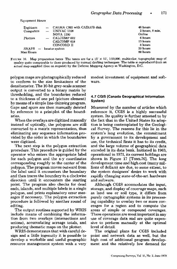
Geographic Data Processing • 171
Eqmpment Hours
Digitizers - - CALMA C985 with CAELUS disk 46 hours Computers - - UNIVAC 1108 2 hours, 8 min.
NOVA 1200 Online Plotters - - CALCOMP 602 6 hours
CALCOMP 618 13 hours CONCORD II 8 hours
SNAPS - - locator system 20 hours Man Hours 80 hours
FIGURE 16. Map preparation times The times are for a 15' × 15', 1:50,000, multicolor, topographic map of quahty quite comparable to those produced by manual drafting techmques The table is reproduced from an actual map supphed (free on request) by the Defense Mapping Agency m Washington, D.C.
polygon maps are photographically reduced to conform to the size limitations of the densitometer. The 10-bit grey-scale scanner output is converted to a binary matrix by thresholding, and the boundaries reduced to a thickness of one pel (picture element) by means of a simple line-thinning program. Gaps and spurs are then manually deleted by reference to a printplot of the bound- aries.
When the overlays are digitized manually instead of optically, the polygons are still converted to a matrix representation, thus eliminating any sequence information pro- vided by the order in which the boundaries were digitized.
The next step is the polygon extraction procedure. This procedure is guided by the operator who enters the appropriate label for each polygon and the x-y coordinates corresponding roughly to the center of the polygon. The program moves outward from the label until it encounters the boundary and then traces the boundary in a clockwise direction until it encounters the starting point. The program also checks for dead ends, islands, and multiple labels in a single polygon, and prints explanatory error mes- sages if necessary. The polygon extraction procedure is followed by another round of editing.
The output routines supported by WRIS include means of combining the informa- tion from two overlays (intersections and unions), accumulating acreage totals, and producing thematic maps on the plotter.
WRIS demonstrates that with careful de- sign and a little ingenuity it is possible to develop a workable and useful geographic resource management system with a very
modest investment of equipment and soft- ware.
4.7 CGIS (Canada Geographical Information System)
Measured by the number of articles which reference it, CGIS is a highly successful system. Its quality is further attested to by the fact that in the United States its adop- tion is being contemplated by the Geologi- cal Survey. The reasons for this lie in the system's long evolution, the commitment by a government to its development and use, the technical firsts it has to its credit, and the large volume of geographical data encoded in its data bank. Initiated in 1963, operational in 1971, its current holdings are shown in Figure 17 [ToML76]. The long development time and high cost (many mil- lions of dollars) are due, to some extent, to the system designers' desire to work with rapidly changing state-of-the-art hardware and software.
Although CGIS accomodates the input, storage, and display of coverage maps, such as land use or soil type, it differs from purely cartographic systems in its process- ing capability to overlay two or more cov- erages for a region and to compute the areas of simple or compound coverages. These operations are most important in any use of coverage data and are quite expen- sive to perform manually at the optimal level of detail.
The original plans for CGIS included point and network data as well, but the high cost of additional program develop- ment and the relatively low demand for
Computing Surveys, Vol 11, No 2, June 1979
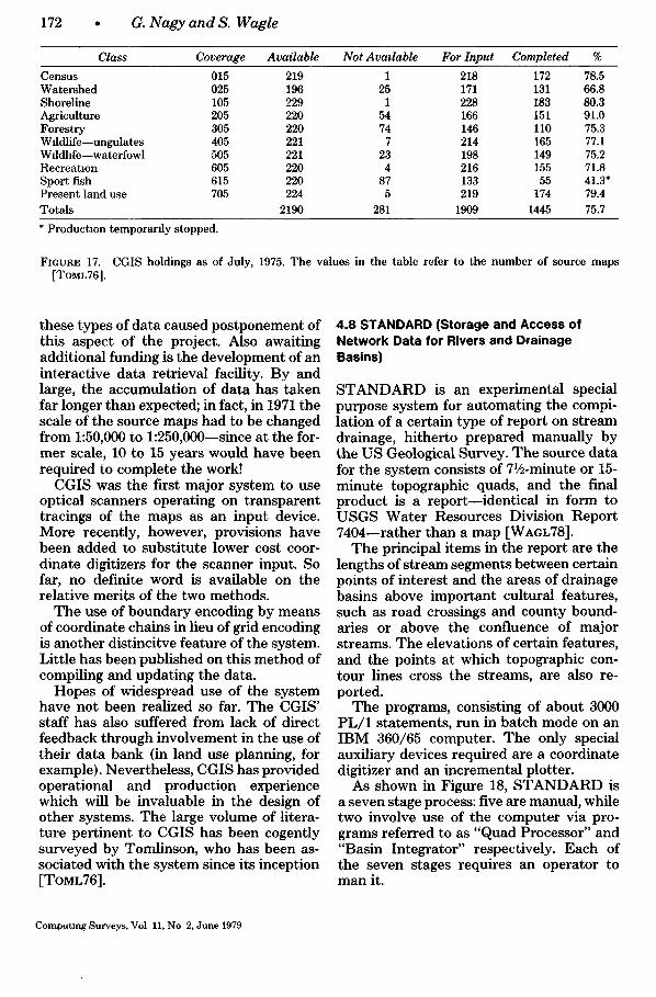
172 • G. Nagy and S. Wagle
Class Coverage Available Not Avadable For Input Completed %
Census 015 219 1 218 172 78.5 Watershed 025 196 25 171 131 66.8 Shoreline 105 229 1 228 183 80.3 Agriculture 205 220 54 166 151 91.0 Forestry 305 220 74 146 110 75.3 Wildlife--ungulates 405 221 7 214 165 77.1 Wfldhfe--waterfowl 505 221 23 198 149 75.2 Recreatmn 605 220 4 216 155 71.8 Sport fish 615 220 87 133 55 41.3" Present land use 705 224 5 219 174 79.4 Totals 2190 281 1909 1445 75.7
* Production temporarily stopped.
FIGURE 17. CGIS holdings as of July, 1975. The values in the table refer to the number of source maps [ToML76].
these types of data caused postponement of this aspect of the project. Also awaiting additional funding is the development of an interactive data retrieval facility. By and large, the accumulation of data has taken far longer than expected; in fact, in 1971 the scale of the source maps had to be changed from 1:50,000 to l:250,000--since at the for- mer scale, 10 to 15 years would have been required to complete the work!
CGIS was the first major system to use optical scanners operating on transparent tracings of the maps as an input device. More recently, however, provisions have been added to substitute lower cost coor- dinate digitizers for the scanner input. So far, no definite word is available on the relative merits of the two methods.
The use of boundary encoding by means of coordinate chains in lieu of grid encoding is another distincitve feature of the system. Little has been published on this method of compiling and updating the data.
Hopes of widespread use of the system have not been realized so far. The CGIS' staff has also suffered from lack of direct feedback through involvement in the use of their data bank (in land use planning, for example). Nevertheless, CGIS has provided operational and production experience which will be invaluable in the design of other systems. The large volume of litera- ture pertinent to CGIS has been cogently surveyed by Tomlinson, who has been as- sociated with the system since its inception [TOML76].
4.8 STANDARD (Storage and Access of Network Data for Rivers and Drainage Basins)
STANDARD is an experimental special purpose system for automating the compi- lation of a certain type of report on stream drainage, hitherto prepared manually by the US Geological Survey. The source data for the system consists of 71/2-minute or 15- minute topographic quads, and the final product is a report--identical in form to USGS Water Resources Division Report 7404--rather than a map [WAGL78].
The principal items in the report are the lengths of stream segments between certain points of interest and the areas of drainage basins above important cultural features, such as road crossings and county bound- aries or above the confluence of major streams. The elevations of certain features, and the points at which topographic con- tour lines cross the streams, are also re- ported.
The programs, consisting of about 3000 PL/1 statements, run in batch mode on an IBM 360/65 computer. The only special auxiliary devices required are a coordinate digitizer and an incremental plotter.
As shown in Figure 18, STANDARD is a seven stage process: five are manual, while two involve use of the computer via pro- grams referred to as "Quad Processor" and "Basin Integrator" respectively. Each of the seven stages requires an operator to man it.
Computing Surveys, Vol 11, No 2, June 1979

MAP/S,
DELINEATION I I
PREOIGITIZATION MARKING I
1 O(GiTIZING ~'1
, ,
OUAD PROCESSING 4l
l TEXT/EOIT ENTRY 51
l I , LIBRARY FILING
1 i 'NTEORA"O I 1
REPORT/S,
FIGURE 18. STANDARD schematic. Only the Quad Processing and Basm Integration stages are strictly automatic. Digitizing and Text /Edi t Entry are in- teractwe, while the other boxes represent manual operations.
Although not shown in the diagram, this process is preceded by a planning stage. During the planning stage the area of inter- est is defined and the set of rivers in the area to be included in the drainage report is listed. The specific maps that will be used to cover the area of interest are also listed. Each of these maps then passes through stages 1 to 5 individually, possibly in par- allel.
Delineation
The segments of rivers from the reporting set that lie in each map are identified. Each of these segments has an associated basin. Using topographic contour information the boundaries of these basins are deduced and marked on the mapsheet.
A segment of a river is that part which lies between two end-of-segment points. The source, river mouth, points of conflu- ence with tributaries, points on map-edges,
Geographic Data Processing • 173
and certain special basin features come under the category of end-of-segment points. Basin features are those features along a river, such as major highway cross- ings, considered significant enough to war- rant determination of the drainage area upstream to them.
Predigitization Marking
The maps contain a considerable amount of information irrelevant to the system. The purpose of this stage is to improve the contrast between relevant and irrelevant information, thus simplifying the design and operation of the next stage of digitiza- tion.
Specifically, arrows are marked pointing out the positions of those features along the rivers which are to be entered. Arrows are also provided to point out the elevation markers along the rivers. The discrete (usu- ally in tens of feet) topographic contour crossings on the rivers and the mouths of the rivers are together called elevatmn markers. The values of elevation markers are also marked at the tail of their arrows. The river and basin boundary traces are numbered for easy sequencing and enumer- ation during digitization. The start and end of these traces are distinctly labeled with these numbers.
Digitization
In this stage an offline digitizer unit is used to record the relevant information on mag- netic tape. The delineated and marked map forms the input to this stage. The operator first enters the map identification (map- name, position on table, etc.), then traces the rivers and basin boundaries as indi- cated, and finally enters the positions of the features and elevation markers--the latter with the elevation values.
Quad Processing
Here the tape files which correspond to a machine-readable form of map information are processed by the Quad Processor. The next stage of Text/Edit Entry also provides the input to Quad Processor in the second and following passes through the loop
Computing Surveys, Vol 11, No. 2, June 1979"

174 • G. Nagy and S. Wagle
formed by stages 3, 4, and 5. The first pass through this loop creates a partial database for this map. In subsequent passes, this partial database is used in conjunction with edit entries to generate an updated version of the database. To compute the geophysi- cal coordinates of the map (latitude and longitude) given its name, a map-index is needed in the first-pass run.
A variety of output that is controllable through a set of options is generated by the Quad Processor. Besides the database just mentioned, this includes schematic maps, a local drainage area report, and details of the database, among others. An important output is a questionnaire aimed at the Text /Edi t entry operator, soliciting the outstanding names of the rivers and fea- tures. These names appear as text in the report, whereas the other details {river length, elevation, basin area, etc.) are de- duced from the digitizer input.
Text~Edit Entry
With the aid of the original marked map and the Quad Processor generated sche- matic maps, the questionnaire just men- tioned is completed. The need for any ed- iting via edit entry or digitizer input is assessed. If additional digitization is neces- sary, the editing instructions are passed to the digitization stage. If the database is deemed adequate, the marked map, the database, the schematic maps and other output from the Quad Processor are passed to the next stage for deposition in the li- brary.
Library Filing
The filing operator is responsible for main- taining the mapsheets and the databases in an organized form. In the current imple- mentation, the library serves as a database holding stage for the individual maps cov- ering the area of interest until all of them are ready for the Basin Integrator stage.
Basin Integration
In this last stage of STANDARD, the da- tabases of the constituent maps covering the area of interest are assembled into an
equivalent database for the entire area. The Basin Integrator generates outputs similar to the Quad Processor including schematic maps and reports.
It is estimated that the manual portions of this process offer a roughly fivefold sav- ings in time and superior accuracy, as com- pared to the former planimeter-and-divid- ers operation.
4.9 GADS (Geo-Data Analysis and Display System)
In terms of flexibility and interactive prob- lem-solving capability, GADS, under devel- opment at IBM since 1973, is unquestiona- bly the most ambitious of the geographical information systems we have examined. Aimed at unstructured problem solving-- where the user does not know, ahead of time, either his data requirements or the specific steps he needs to take to approach the solution, GADS provides advanced in- formation retrieval, programming, statisti- cal analysis, and display facilities for urban applications. The system has been sub- jected to limited operational testing by mu- nicipal agencies interested in the optimal reconfiguration of police beats and school districts, with further applications planned in urban forecasting and for solving certain network-related (as opposed to area-re- lated) problems [CARL74, MANT74, NIEM 78].
The GADS user interface accomodates a variety of devices such as keyboards, a re- freshed color display scope, joystick and cursor, lightpen, storage tube, and incre- mental plotter. There is also provision to project source maps over a display screen, either to provide a detailed backdrop for a computer display or to digitize map infor- mation [GIDD73].
The basic geographic units in GADS are called zones. Zones may be defined either as strictly geometric entities such as uni- form squares, or they may correspond to units natural to the application at hand, such as city blocks or school districts. In particular, the DIME Geographic Base File (see Section 4.3) is often used to provide the necessary locational framework.
Attractive and colorful as the GADS ter-
Computing Surveys, Vol 11, No 2, June 1979

minals are, the system's major contribution is its sophisticated data management facil- ity. This may be no accident, since for several years the development team occu- pied quarters next door to IBM's database research group!
As shown in Figure 19, the database is organized in two levels. The large, complete database is never directly accessed by the user; instead, support personnel extract a mini data15ase for each user. The data ma- nipulation and display subsystems operate
Geographic Data Processing • 175
solely on the extracted data. This has sev- eral advantages:
1) The integrity of the main database is protected from user error (and, possibly, user curiosity).
2) The extracted mini database may be small enough to allow the analysis to be performed on a small computer instead of the large--and possibly distant--host ma- chine [CARL75].
3) The efficiency of retrieval is improved and the software for managing the ex-
OlSpley
Ll0ht Pen
i
ANALYSIS AND DISPLAY FUNCTIONS Statement Language Map Display Overlay Graphs Contruct~on
Table Display and Correction
Example of Tables m Extracted Data Base
~ Year I 0 I Data Access [ Year 2 Program I
/ I . I I Year I l Cr,mes Crimes Houses Populat,on / ~: I z°ne J #I #2 , - - / / Z/Extracted / / I 1 I 3 15 50 146
Data 3 4 4 41 192
I Create and I / i lan d I /~Extract,on ~ I Modify I / I - I = ' Specification I Program J I Subset.t'ng ~ ' ~ ,
X,Y Coded Data~des I EXTRACTION
/ Spec I - P M , , 7 I " urpose aps I Geographic Code I I ~Detalled \ hi to Geographic [ I \Base Map • " Coordinate |
I Transformation / I Geographic ~ i Base Fi e J
ion • se DATA F,,ES
FIGURE 19. GADS schemat ic . T h e mos t notable feature of GADS is the insulat ion of users f rom the ma in da tabase th rough the extract ion of a speciahzed mini da tabase for each user [CARL74].
Computing Surveys, Vol 11, No 2, June 1979

176 • G. Nagy and S. Wagle
tracted database can therefore be simple- minded.
4) The user may view the extracted da- tabase as a set of named tables. This view corresponds to the relational model of da- tabase organization [CODD70].
Because of heavy computer processing requirements, the relational model has not been implemented in the large original da- tabase. This need not, however, trouble the user, since his activities are confined to the mini database. Nor does he have to worry about coordinate transformation, aggrega- tion, and subsetting operations necessary to represent his data according to the zone structure specified by his base map; that is all taken care of during the extraction proc- ess!
He can, however, using a simple com- mand language reminiscent of BAsic, dis- play the attributes associated with each zone by symbol, color, or density; create new attributes by arithmetic or logical op- erations; examine and update any table; and combine zones to create superzones. He may also plot one variable against an- other, obtain tabular displays of the data, and perform statistical computations. Fi- nally, he can save the sequences of com- mands necessary to perform these actions, and gradually build up his own "program" library.
It is easy to see that human-factors con- siderations played a paramount role in the design of GADS, and no effort was spared to develop a user-friendly interface. In spite of this, some guinea pigs, recruited from outside the realm of computers, find the system demanding and capricious, and left to themselves revert to primitive means of decision making.
4.10 NIMS
Aided by the availability of records system- atically kept by the parish and local au- thorities on the locations of individuals and real estate, Sweden gained an early lead in geographical data processing [NORD72, SALO69]. This lead is being maintained through systems such as NIMS [RoaN76].
Unlike GADS, where street addresses have to be translated to geographical coot-
dinates, the objects in NIMS already carry their coordinates. The NIMS data bank contains information on individuals and real estate, called "outlets." The data on individuals is characterized by age, sex, oc- cupation, and income, among other attri- butes. The outlets can be classified on the basis of their type (e.g., store) and capaci- ties. The system also keeps nonpoint infor- mation such as permanent geographical areas (e.g., towns and housing areas) and road networks. The user can, on a tempo- rary basis, enter additional areas (polygons) or segments to suit his application.
The user at a terminal formulates his query interactively with guidance from the system. He then has the option of having the extracted data listed, tabulated or dis- played in the form of maps or graphs. In any case, the query becomes the input to a program which executes in batch mode, and the user receives the output later in the day. While the lack of interactive execution does not allow data exploration as in GADS, this is compensated by the ability to formulate quite complex queries, as de- scribed below.
There are twelve basic types of retrieval options available in NIMS. Included in these are retrieval of objects of a specified type that lie within a predefined areal unit and retrieval based on the distance from a set of segments, such as a road or pipeline network. This already powerful set is fur- ther enhanced by a feature which allows two independent basic retrieval options to be specified simultaneously, the result being some overlay of the two sets. In effect, the user has a rich set of 144 different types of retrieval available to him. Although this set is more general than that available in any other system, it seems to be biased towards planning applications where the facilities (outlets and roads), treated as re- sources, have to be optimally distributed among their potential customers.
"Dependent outlet in topologically de- limited areas with distance zones along routes" is a type of complex query and is coded 0509, since it is a combination of basic retrieval options of type 5 and 9. An example query of this type is, "Which pup- ils, living over 2 km from their nearest
Computing Surveys, Vol II, No 2, June 1979

primary school area (05), are also over 1.5 km from a bus route (09) and how are they distributed in distance classes?" On most systems this query would require develop- ment of a special program. On NIMS it can be formulated by the end user. In this re- spect, at least, it can be said that NIMS provides a query language for geographical data.
CONCLUSION
What this paper purports to show is that geographical data processing has much in common with conventional business data processing, and yet enough distinctive fea- tures of its own to merit consideration as a separate field. The similarities include:
1) Both are in a period of rapid develop- ment, though the total volume of business data processing is now, and likely to remain, orders of magnitude larger than geograph- ical data processing.
2) Both are characterized by vast amounts of data and complex relationships between data elements. Both will be af- fected and enhanced by current develop- ments in database technology.
3) Common to both is the importance of a stable, reliable production environment in order for day-to-day operations to be incorporated into the mainstream of orga- nizational activity (the GDP lagging, of course).
4) There exists an obvious yet neglected need for more detailed planning, better management, and more thorough docu- mentation, with the GDP again lagging in adopting modular program development techniques such as top-down design and structured programming.
5) Both are tending towards interactive information retrieval with intelligent ter- minals or maxi-mini configurations.
Because of these similarities, GDP has much to learn from the best of the business DP systems and from relevant research in computer science. The features which ren- der GDP distinctive are:
1) In geographical applications the loca- tional attributes play an important role. The inherently two-dimensional nature of
Geographic Data Processing • 177
GDP profoundly influences data organiza- tion, algorithm design, and input-output. These considerations also lead to exciting new research problems in computational geometry, operations research, and image processing.
2) There is no known sufficient set of primitive operations (such as +, - , *, /, , •, , and assignment for integers) for geo- graphic data types.
3) Geographic entities tend to require an indeterminate amount of storage.
4) Most GDP systems are in government rather than private hands because major applications are in large area planning, in- cluding natural resource management and facility location. Government funding has not yet however resulted in significant standardization (except in cartography).
5) There is a lack of large commercially developed software systems which could establish the cost-effectiveness of GDP sys- tems.
6) Contributors are drawn mainly from the academic and scientific community (earth sciences and social sciences) rather than the business world, resulting in slower than expected conversion of prototype de- signs to operational systems [RHIN77].
7) GDP involves the use of specialized and expensive input-output equipment. Co- ordinate digitizers and incremental plotters have probably reached a plateau with re- gard to price and performance, but optical scanners and graphic display devices are still subject to considerable technical de- velopment and possible price reductions.
8) The maturing technology of remote sensing is likely to have considerable im- pact on GDP.
The number of disciplines and fields which bear on geographical data processing ensure its continuing vigor and progress. Although we have tried to present a state- of-the-art survey, we hope and believe that new developments will soon render most of our material obsolete.
ACKNOWLEDGMENTS
This work represents part of a continuing project supported by the Nebraska Water Resources Center, Natural Resources Commission, Depar tment of Ad-
Computmg Surveys, Vol 11, No 2, June 1979

178 • G. N a g y a n d S. W a g l e
mmistrative Services, the Old West Commission, the Conservation and Survey Division, and the Maude Hammond Fling Fellowship Fund of the Umversity of BERN76 Nebraska The help of LuAnn Murray, Marjorie Reid, and Audrey Schardt in the preparation of the manu- script, under National Aeronautics and Space Admin- BERN78 istration grant NGL 28-004-020, is also gratefully ac- knowledged. BICK64
On the technical plane we are indebted to Drs. George Corliss and Frank Burton for valuable sugges- tmns on the original manuscript, and to the ACM BIRK69 referees for a number of detatled recommendations and additional references
ACSM74
ALDR72
ALDR75
ALVA74
ANUT69
ANUT77
ASP75
AYER74
BAKI71a
BAKI71b
BANS78
BENT76
BERN71
REFERENCES BOYL72
AMERICAN CONGRESS SURVEYING & MAPPING (ACSM), Proc. Int. Conf Au- tomatmn ~n Cartography, 1974. Aldred, B K. Points ~n polygon algo- rithms, Rep UKSC 0025, IBM (UK) Sci- BOYL74 entific Center, Peterlee, 1972. Aldred, B. K. (Ed) Proc. IBM UK Sct. ent~ftc Center Seminar Geographical Data Processing, Rep. UKSC 0073, IBM BOYL76 (UK) Scientific Center, Peterlee, 1975. ALVAREZ, D. T. AND TAYLOR, M. L. Cartographic data base hLerarchy, BRAS77 Vols. I, II and III, PRC Information Sci- ence Co, McLean, Va., Sept 1974. ANUTA, P. E. "Digital registration of multlspectral video imagery," SPIE J 7 (1969), 168-175 BREE42 ANUTA, P. E, "Computer-associated analysis techniques for remote sensing BURT77a data interpretation," Geophysics 42, 3 (1977), 468-481. AMERICAN SOCIETY OF PHOTOGRAMME- TRY (ASP), Manual of remote sensing, Vols. 1 and 2, ASP, Fails Church, Va., 1977. AYERS, L. F. A review of cartographic automation, Defense Mapping Agency, Aerospace Center, Washington D.C, 1974. BAKIS, R., WESLEY, A., AND WILL, P. M. "Digital image processing for the BURT78 Earth Resources Technology Satellite data," in Proc. IFIP Congress 71, Elsev- ier North-Holland, Inc., New York, 1971. BAKIS, R. "Digital correction of geo- metrm and radiometrie errors m ERTS data," m Proc 7th Int. Syrup Remote Sensing of Enwronment, 1971, Center for CALK77 Remote Sensing Information and Analy- sis, Willow Run Laboratories, Umv. of Michigan, Ann Arbor, 1427-1436. BANSAL, M. Nebraska natural re. sources data bank ~nformatmn system, Nebraska Natural Resources Commis- CARL74 sIon, Lincoln, Neb., March 1978. BENTLEY, J L., AND SRAMOS, M. I. "Divide-and-conquer in multidimen- sional space," in Proc. 8th Annual ACM Syrup Theory of Computing, ACM, New CARL75 York, 1976, 220-230. BERNSTEIN, R., AND SILVERMAN, H F. "Digital techniques for earth re- source image data processing," presented
BURT77b
CHAM47
at the AIAA 8th Annual Meeting, Sept. 1971, also IBM-FSD Tech. Rep. FSC 71- 6017, Galthersbur,~, Md. BERNSTE1N, R. Digital image process- ing of earth observation sensor data," IBM J. Res. Dev. 20, 1 (Jan. 1976). BERNSTEIN, R (Ed) D~gttal ~mage processing for remote senslng, IEEE Press, New York, 1978. BICKMORE, D P., AND BOYLE, A. R "An automated system of cartography," in Tech Syrup. Int Cartography Assoc., Edinborough, 1964 BIRKHOFF, G. "Plecewlse bicubic inter- polation and approximation in polygons," In Approxlmatmn w~th specml emphas~s on sphne functions, I. J. Schoenberg (Ed.), Academic Press, New York, 1969 BOYLE, A. R. "Equipment for spatial data processing," in Geographwal data handhng, Vol. 2, R. F. Tomlinson (Ed.), IGU Commission on Geographical Data Sensing and Processing, Ottawa, Ont., 1972. BOYLE, A R "Geographic information systems in hydrography and oceanogra- phy," Can. Cartogr II, 2 (Dec 1974), 125-141. BOYLE, A R. "The requirements of an interactive display and edit facdlty for cartography," Can. Geogr. 13 (1976). BRASSEL, K A survey of cartographtc d~splay software, Rep. R-77/3, Geo- graphic Information Systems Labora- tory, State Univ. of New York, Buffalo, 1977. BREED, C.B. Surveying, John Wdey & Sons, Inc., New York, 1942 BURTON, W. "Representation of many- sided polygons and polygonal lines for rapid processing," Commun. ACM 20, 3 (March 1977), 166-171 BURTON, W. "Efficient retrieval of geo- graphical information on the basis of lo- cation," m Proc. Advanced Study Symp. Topological Data Structure for Geo- graphic Informatmn Systems, G. H. Dut- ton (Ed.), Harvard Univ. Laboratory for Computer Graphics and Spatial Analysis, Cambridge, Mass., 1977. BURTON, W "A fLxed grid curve repre- sentation for efficient processing," in Proc SIGGRAPH '78, Ftfth Annual Conf. Computer Graphtcs and Interac- twe Techniques, ACM, New York, 1978, 64-69. Pubhshed as Comput Gr 12, 3 (Aug. 1978) CALKINS, H. W, AND TOMLINSON, R F Geographtc informatton systems, methods, and equipment for land use planning, IGU Commission on Geo- graphical Data Sensing and Processing, Ottawa, Ont., Aug. 1977. CARLSON, E. D., ET AL. The design and evaluatmn of an ~nteractwe geo-data analysts and display system, Rep. RJ 1342, IBM Research Laboratory, San Jose, Calif, 1974. CARLSON, E.D. Using large data bases for mteracttve problem solvmg, Rep. RJ 1585, IBM Research Laboratory, San Jose, Cahf., 1975. CHAMBERLIN, W. The round earth on
Computing Surveys, Vol 11, No 2, June 1979

CHAS78
CLAI73
CODD70
COTT69
CRAN72
DACE70
DALE74
DATE75
DAVI75
DEET77
DELF75
DEO74
DIEL72
DOBK76
DUDA73
DUEK77
DUTT77
fiat paper, National Geographic Society, Washington, D.C., 1947. CHASEN, S. H. Geometrw principles and procedures for computer graphzc ap- phcatmns, Prentice-Hall, Inc., Engle- ECU71 wood Cliffs, N.J , 1978 CLAIRE, C N State plane coordinates by automatw data processing, C&GS Pub. 62-4, US Dept. Commerce, Environ- FRED74 mental Science Administration, Wash- ington, D.C., 1973. CODD, E. F "A relational model of data for large shared data banks," Commun. ACM 13, 6 (June 1970), 377-387. COTTAFAVA, G., AND LEMOLI, G. FREE74 "Automatic contour map," Commun ACM 12, 7 (July 1969), 386-391. CRANE, C. M. "Contour plotting for FUCH77 functions specified at nodal points of an irregular mesh based on an arbitrary two- parameter coordinate system," Comput. J. 15 (1972), 382-384. GIDD73 DACEY, M.F. "The syntax of a triangle and some other figures," Pattern Recogn. 2 (1970), 11-31. DALE, P F. (ED.) Automatmn ~n car- tography, British Cartographic Society, GILB77 1974. DATE, C. J. An mtroductmn to data- base systems, Addison-Wesley Publ. Co., GILO78 Reading, Mass., 1975. DAVIS, J. C, AND McCULLAGH, M J. (EDs.) Dzsplay and analysis of spattal HARV77 data, John Wiley & Sons, Inc., New York, 1975. DEETZ, C H., AND ADAMS, O . S . Ele- ments of map prolectmn wtth apphca- ttons to map and chart constructmn, Greenwood Press, Inc., Westport, Conn., HARV78 1977. DELFINER, P., AND DELHOMME, J P "Optimum interpolation by Knng- ing" in Dzsplay and analysts of spatial data, J. C Davis and M. J. McCuUagh, HORO78 (Eds), John Wiley & Sons, Inc., New York, 1975. DEO, N. Graph theory wtth apphca- tmns to engzneerzng and computer sc~- IGU77a ence, Prentice-Hall, Inc, Englewood Cliffs, N.J , 1974 DIELLO, J Experimental cartography at the Rome A~r Development Center, Rome Air Development Center, Rome, IGU77b N. Y., 1972. DOBKIN, D, AND LIPTON, R. J. "Multidimensional searching problems," KELK74 SIAM J Comput 5 (1976). DUDA, R., AND HART, P. Pattern clas- s~fwatmn and scene analysts, John Wiley & Sons, Inc., New York, 1973. LACI78 DUEKER, K. J., AND NOYNAERT, J E. Interactwe dtg~t~zmg, edttmg, and mapping: software and data structure LEE76 constderattons, Tech Paper 92, Inst Ur- ban and Regional Research, Univ. of Iowa, July 1977. DUTTON, G.H. "Navigating Odyssey," in Proc. Advanced Study Syrup Topol- LEWI76 ogwal Data Structures for Geographical Informatmn Systems, G. H Dutton (Ed), Harvard Univ Laboratory for LIEn76 Computer Graphics and Spatial Analysts, Cambridge, Mass., 1977. LOOM65
Geographw Data Processing • 179
DUTT78 DUTTON, G. H., AND NISEN, W.G. "The expanding realm of computer cartogra- phy," Datamatmn 24, 6 (June 1978), 134- 142. EXPERIMENTAL CARTOGRAPHY UNIT, (ECU) Automatic cartography and planning, Architecture Press, London, 1971. FREDEN, S C., ET. AL., (EDs.) "Discipline summary reports," in Proc. Thtrd Earth Resource Technology Syrup, Rep. SP-357, Scientific and Tech- nical Information Office, NASA, Wash- ington, D C., 1974. FREEMAN, H. "Computer processing of line drawing images," Comput Surv. 6, 1 (March 1974), 57-97. FUCHS, H., KEDERN, Z M., AND USEL- TON, S P "Optimal surface reconstruc- tion for planar contours," Commun. ACM 20, 10 (Oct. 1977), 693-702 GIDDINGS, G M, AND CARLSON, E G. An ~nteractive system for creating, edit- ing and d~splay~ng a geographw base file, Rep RJ 1288, IBM Research Labo- ratory, San Jose, Calif, 1973. GILB, T., AND WEINBERG, G Human- tzed ~nput, Winthrop Publ. Inc., Cam- bridge, Mass., 1977. GILOI, W. K Interactwe computer graphws, Prentice-Hall, Inc, Englewood Cliffs, N.J , 1978 Proc Advanced Study Syrup Topolog- tcal Data Structures for Geographical Information Systems, G. H Dutton (Ed), Harvard Univ. Laboratory for Computer Graphics and Spatial Analysis, Cambridge, Mass., 1977. Int Users" Conf. Computer Mapping Software and Data Bases. Apphcatton and Dissem~natmn, Harvard Univ. Lab- oratory Computer Graphics and Spatial Analysis, Cambridge, Mass, 1978 HOROWITZ, E , AND SAHNI, S. Funda- mentals of computer algorithms, Com- puter Science Press, Woodland Hills, Calif., 1978. INT GEOGRAPHICAL UNION, Dwectory of mdw~duals m the field of geographi- cal data handling, The Lands Directo- rate, Dept of Fisheries and Environment, Government of Canada, Ottawa, 1977. INT GEOGRAPHICAL UNION, Computer software for geographical data han- dhng, UNESCO Press, New York, 1977 KELK, B. "Hardware for automated cartography," in Automatmn in cartog- raphy, British Cartographic Society, 1974 Proc. LACIE Symp., J.SC-14551, 14700, 14557, NASA LBJ Space Center, Hous- ton, Texas, 1978. LEE, D. T , AND PREPARATA, F P "Location of a point In a planar sub- division and its applications," in Proc 8th Annual ACM Syrup Theory of Comput- tng, ACM, New York, 1976, 231-235. LEWIS, ET AL. Compder design theory, Addison-Wesley Publ. Co., Reading, Mass., 1976. LIEBENBERG, E "SYMAP Itsuses and abuses," Cartogr. J. 13 (1976). LOOMIS, R. G. "Boundary networks,"
Computing Surveys, Vol 11, No 2, June 1979

180
MCLA74
McLE74
MANT74
MARK71
MART77
MENE76
MERR73
MILL68
MOST69
MORS69
NAOY72
NAGY 79
NEWM73
NIEM78
NORD72
PALM75
PARN72
PAVL72
G. Nagy and S. Wagle
Commun. ACM 8, 1 (Jan 1965), 44-48. McLAIN, D. H. "Drawing contours from arbatrary data points," Comput. J. 17 (1974), 318-324. PEUC77 McLELLAN, W. G., AND MORITZ, B. K. An mteractwe on-line mult~-mmwom- puter configuration for application to PEUQ77 cartography, PRC Information Sciences Co., McLean, Va., 1974. MANTEY, P. E. Transportatton plan- ning apphcations of the geo-data anal- ysts and dtsplay system, Rep. RJ 1459, PFAL67 IBM Research Laboratory, San Jose, Calif., 1974. MARKARIAN, H., BERNSTEIN, R, FER- NEYHOUGH, D. G., GREGG, C. E., AND PFAL72 SHARP, F.E. "Implementation of digital techniques for correcting high resolution RABI76 nnages," presented at the ASP-ACSM Fall Conventton, 1971, also IBM-FSD, Tech. Rep. FSC 71-6012, Gaithersburg, Md RmN75 MARTIN, J. Computer data.base orga- mzaaon, Prentice-Hall, Inc., Englewood Chffs, N.J., 1977. RHIN77 MENELEY, G.J . Place coding" raven- tory, analysis, and recommendations, Teeh. Rep. No. 73, Inst. Urban and Re- RICH72 gional Research, Univ. of Iowa, 1976. MERRILL, R. D. "Representation of contours and regions for efficient com- puter search," Commun. ACM 16, 2 (Feb. RONN76 1973), 69-82. MILLER, W. F, AND SHAW, A. C. "Lingmstie methods in pmture proc- essing--a survey," m Proc. AFIPS 1968 Fall Jt. Computer Conf., Vol. 33, Part 1, ROBI69 Thompson Book Co., Washington, D.C., 279-290. MONTANARI, U. "Continuous skeletons RADC72 from digitized images," J. ACM 16, 4 (Oct. 1969), 534-549. MORSE, S P. "Concepts of use in con- tour map processing," Commun. ACM ROSE66 12, 3 (March 1969), 147-152 NACY, G. "Digital image-processing ac- tivities in remote sensing for earth re- sources," Proc. IEEE 60 (1972), 1170- ROSE69 1200. NA(;Y, G., AND WAGLE, S. "Ap- proximation of polygonal thematm maps RosE71 by cellular maps," Commun ACM, to appear. NEWMAN, W. M., AND SPROUL, R. F. Principles of Interactive computer RosE76 graphics, McGraw-Hill, New York, 1973. NIEMEYER, G. "Dispatching by graphi- cal terminals," Comput. Gr. 11, 4 (March Russ75 1978), 58-66. NORDBECK, S., AND RYSTEDT, B. Computer cartography, Studentlittera- tur, Lund, Sweden, 1972 PALMER, J. A B. "Computer science SALO69 aspects of the mapping problem," in Dts- play and analysis of spattal data, J C Davis and M. J. McCullagh (Eds.), John Wiley & Sons, Inc., New York, 1975. SCHM75 PARNAS, D. "On the criteria to be used m decomposing systems into modules," Commun. ACM 15, 12 (Dec. 1972), 1053- 1058. PAVL1DIS, W. "Piecewise approximatmn of functmns of two variables through re-
glons with variable boundary," in Proc. ACM National Conf., 1972, ACM, New York. PEUCKER, T. K. Computer cartogra- phy: a working btbhography, Dept. Georgraphy, Univ. of Toronto, 1972 PEUQUET, D.J . Raster data handhng in geographw reformation systems, Rep. R-77/7, Geographic Information Systems Laboratory, State Umv. of New York, Buffalo, 1977. PFALTZ, J. L, AND ROSENFELD, A. "Computer representation of planar regions by their skeletons," Commun. ACM 10, 2 (Feb. 1967), 119-122. PFALTZ, J. L. "Graph structures," J. ACM 19, 3 (July 1972), 411-422. RABIN, M. O "Probabilistic algo- rithms," in Algorithms and complemty, J. F. Tranb (Ed), Academic Press, New York, 1976. RHIND, D.W. "A skeletal overvmw of spatial interpolation techniques," Corn- put. Appl. 2 (1975) RHIND, D.W. "Computer aided cartog- raphy," Trans. Inst. Br~ttsh Geogr. New Series 2, 1 {1977), 71-96. RICHARDUS, P., AND ADLER, R. K Map proyectmns for geodetists, cartogra- phers, and geographers, American El- sevier, New York, 1972. RONNBERG, A. O. S., AND SELANDER, K. NIMS methods of area analysts, Working Paper No. 8, SORSA--Int. Seg- ment Oriented Referencing System Or- gamzation, Stockholm, 1976. ROBINSON, A. d., AND SALE, R. D Elements of cartography, John Wiley & Sons, Inc, New York, 1969. ROME AIR DEVELOPMENT CENTER, A compendium of techmcal papers on ex- periments tn cartography at Rome Aw Development Center, Rome, N.Y, 1972. ROSENFELD, A., AND PFALTZ, d. L. "Sequential operations m digital pic- ture processing," J. ACM 13, 4 (Oct. 1966), 471-494. ROSENFELD, A Picture processing by computer, Academic Press, New York, 1969. ROSENFELD, A. "Isotonic grammars, parallel grammars, and picture gram- mars," in Machine intelligence VI, American Elsevmr, New York, 1971. ROSENFELD, A. AND KALE, D. D~g~tal pwtureprocessmg, Academm Press, New York, 1976 RUSSELL, R. M., SHARPNACK, D. A., AND AMIDON, E L. WRIS: a resource mfor. matron system for wddltfe management, Res. Paper PSW-107, USDA Forest Ser- vice, 1975. SALOMONSSON, O., ALFREDSSON, B., AND SELANDER, K. FRIS A" a spattal mfor- matron system, Central Board for Real Estate Data, Sundbyberg, Sweden, 1969. SCHMIDT, A. H., AND ZAFFT, W. A. "Programs of the Harvard Univer- sity Laboratory for Computer Graphics and Spatial Analysis," in Dtsplay and analysts of spatml data, J. C. Davis and M. J McCullagh (Eds), John Wiley & Sons, Inc., New York, 1975.
Computing Surveys, Vol 11, No 2, June 1979

Geographic Data Processing * 181
SELI78
SHAM75
SILV77
SPRU75
STRUT5
TAYL76
TEIC78
THIE75
THOM66
THOR77
SELIGMANN, J., FOOTE, J., AND BEGLEY, S. "Mapping with a computer," News- week, (Sept. 11, 1978), 87. SHAMOS, M.I. "Geometric complexity," m Proc. 7th Annual ACM Syrup Theory of Computtng, ACM, New York, 1975, TOBL59 224-233. SILVER, J. The GBF/DIME system: de- velopment, design and use, US Bureau TOBL62 of the Census, Washmgton, D.C., 1977. SPRUNT, B.F. "Rehef representation in automated cartography: an algorithmic TOBL75 approach," in Dtsplay and analysts of spattal data, J. C. Davis and M . J . TOML70 McCullagh (Eds.), John Wiley & Sons, Inc., New York, 1975. STRUCK, R.L. Makmg a map wtth dtg- ttal data, Defense Mapping Agency, TOML72 Topographic Center, Washington, D.C., 1975. TAYLOR, D. R. F. (ED.) Proc Syrup. Geographtc Informatton Processzng, TOML76 Dept. of Geography, Carleton Univ., Ot- tawa, Ont., 1976. TEICHOLZ, E. "Processing satelhte WAGL78 data," Datamatton 24 (June 1978), 117- 132. THIERAUF, R J , AND KLEKAMP, R. C. Dectston maktng through operattons re- search, John Wiley & Sons, Inc., New WARD78 York, 1975 THOMPSON, M M. (ED.) Manual of photogrammetry, American Society of WATS71 Photogrammetry, Falls Church, Va, 1966. WILL70 THORPE, L. W. "Cartographic data structures in productmn use at exper~- mental cartographic unit," in Proc. Ad- vanced Study Syrup. Topological Data
Structures for Geographical Informa. tton Systems, G. H. Dutton (Ed.), Har- vard Univ. Laboratory for Computer Graphms and Spatial Analysis, Cam- bridge, Mass., 1977. TOBLER, W. R. "Automation and car- tography," Geogr. Rev. 49 (1959), 526- 534 TOBLER, W.R. "A classification of map projections," Annu. Assoc. Am Geogr. 52 (1962), 167-175. TOBLER, W. K "Analytical cartogra- phy," Am. Cart ogr. 3 (1975), 21-31. TOMLINSON, R. F. (ED.) "Environment reformation systems," in Proc. UNESCO/IGU First Symp. Geographt- cal Information Systems, 1970 TOMLINSON, R F. (ED.) ~eographtcal data handhng, Vols. 1 and 2, IGU Com- mission on Geographical Data Sensing and Processing, Ottawa, Ont., 1972. TOMLINSON, R. F. (ED.) Computerhan- dhng of geographtcal data, UNESCO Press, Paris, 1976. WAGLE, S.G. "Issues in the design of a geographical data processing system: a case study," PhD Dissertation, Dept. Computer Science, Univ. of Nebraska- Lmcoln, 1978. WARD, S A. "Real time plotting of ap- proximate contour maps," Commun. ACM 21, 9 (Sept 1978), 788-790. WATSON, G. S. "Trend-surface analy- sis," J , Math Geol 3, 3 (1971). WILL, P. M., BAKIS, R., AND WESLEY, M. A. On an all-dtgttal approach to Earth Resources Satelhte image processmg, IBM Tech. Rep. RC-3027, IBM, York- town Heights, N.Y, 1970
RECEIVED APRIL 1978. FINAL REVISION ACCEPTED FEBRUARY 1979
Computing Surveys, Vol 11, No. 2, June 1979