geographical location optimisation of wind and solar ... · solar photovoltaic power and load...

Geographical Location Optimisation of Wind and Solar

Photovoltaic Power Capacity in South Africa using Mean-

variance Portfolio Theory and Time Series Clustering

By

Christiaan Johannes Joubert

November 2016

Thesis presented in partial fulfilment of the requirements for the degree

Master of Engineering in Electrical Engineering at Stellenbosch University

Supervisor: Prof. H.J. Vermeulen

Department of Electrical and Electronic Engineering

i

Declaration

By submitting this thesis/dissertation electronically, I declare that the entirety of the work contained

therein is my own, original work, that I am the sole author thereof (save to the extent explicitly

otherwise stated), that reproduction and publication thereof by Stellenbosch University will not

infringe any third party rights and that I have not previously in its entirety or in part submitted it for

obtaining any qualification.

C.J. Joubert

November 2016

Copyright © 2016 Stellenbosch University

All rights reserved

ii

Acknowledgements

I would like to thank the following people for their contribution during this project:

My study leader, Prof H.J. Vermeulen, for his valuable guidance and inputs throughout my two

years at Stellenbosch University. Thanks are also due to Prof H.J. Vermeulen’s family who opened

up their home to the crowd of master’s students and their circle of friends on many occasions.

My mother, Marina Joubert, father, Stefan Joubert, brother, Peter Joubert, aunt, Juanita Du Toit,

grandmother, Irene Du Toit, as well as my late grandparents Pieter du Toit, Chris Joubert and Rita

Joubert. To the extent that I have achieved anything in my life it would undoubtedly not have been

possible without their unwavering love, sacrifice and support.

Yoko Yuan, who showed enormous patience and strength while waiting for two years for me to

complete my master’s.

All my fellow masters students in room E222, Almero de Villiers, George Blignault, Edwin

Mangwende, Vicki Vermeulen and Tielman Nieuwoudt who made my time in Stellenbosch

unforgettable.

The director of the Centre for Renewable and Sustainable Energy Studies at Stellenbosch

University, Prof J.L. Van Niekerk, who awarded me a bursary which enabled me to pursue a

master’s degree and switch to a career in renewable energy.

Karin Kritzinger, a researcher at the Centre for Renewable and Sustainable Energy Studies at

Stellenbosch University, for being a friend and an enthusiastic supporter of my work and future

career plans.

Dylan Jacklin, an old friend from the residence in Pretoria who joined me in Stellenbosch in 2016

and who made sure that a printed copy of this thesis reached my study leader while I was attending

a conference in Malaysia.

My industrial mentor, Riaan Smit from Eskom, who patiently listened to my project updates and

helped me whenever I needed any data from Eskom.

iii

Abstract

Throughout the world, there is a lot of pressure on governments and electricity utilities to try to

mitigate the possible effects of climate change by reducing emissions of greenhouse gases and

investing in renewable energy sources. Wind power and solar photovoltaic power represent the bulk

of the installed renewable energy capacity. However, these energy sources are stochastic and highly

dependent on weather conditions and exhibit marked diurnal and seasonal cyclic behaviour. It follows

that power systems with a high penetration of wind and solar power present challenges to grid

operators in the sense that renewable power cannot be dispatched on demand as is the case with

conventional power generation plants.

There are several studies in the literature which investigate the possibility of optimising the location

of wind farms so as to reduce the variability of the cumulative wind power output. The majority of

these studies employ mean-variance optimisation, which is a quadratic programming method that is

used in finance theory to construct efficient share portfolios. Several studies suggest the inclusion of

solar photovoltaic power and load profiles in the mean-variance optimisation procedure, but little

work has been done to investigate the effects. A problem with the mean-variance optimisation is that

it often assigns low capacities to certain sites, with no clear alternatives, which makes part of its

solution unfeasible in the face of practical and economic considerations. Time series clustering has

been suggested as a possible solution to this problem, but the literature is sparse when it comes to

time series clustering implementations combined with mean-variance optimisation.

In this investigation, wind power and solar photovoltaic power time series were simulated for a South

African case study. An optimal clustering methodology was identified for the simulated renewable

power time series and the results of the clustering procedure was used as an input in a mean-variance

optimisation procedure that was adapted to include wind power, solar photovoltaic power and load

profiles.

The complete optimisation methodology has been studied in four case studies using clearly defined

key performance indicators. The results of the case studies are a clear indication of the potential of

methodology to optimally distribute wind power and solar photovoltaic power capacity that could

reduce the adverse impacts on the conventional generation capacity that are typically associated with

large penetrations of renewable power capacity.

iv

Opsomming

Regoor die wêreld is daar 'n baie druk op regerings en elektrisiteitmaatskappye om te probeer om die

moontlike gevolge van klimaatsverandering te versag deur die vrystelling van kweekhuisgasse te

verminder en te belê in hernubare energiebronne. Windkrag en fotovoltaïese sonkrag verteenwoordig

die grootste deel van die geïnstalleerde kapasiteit van hernubare energie. Maar hierdie energiebronne

is stogastiese en baie afhanklik van weerstoestande en toon duidelike daaglikse en seisoenale sikliese

gedrag. Dit volg dus dat kragstelsels met 'n hoë penetrasie van wind- en sonkrag ’n uitdaging

verteenwoordig aan kragstelseloperateurs in die sin dat hernubare krag nie kan gewek word op

aanvraag soos in die geval van konvensionele kragopwekkingstasies nie.

Daar is verskeie studies in die literatuur wat die moontlikheid ondersoek van die optimering van die

ligging van windplase ten einde die wisselvalligheid van die kumulatiewe windkraglewering te

verminder. Die meerderheid van hierdie studies gebruik sogenaamde gemiddelde-variansie

optimering, wat ’n kwadratiese programmeringmetode is wat gebruik word in die finansiële teorie

om doeltreffende aandeleportefeuljes te bou. Verskeie studies dui na die insluiting van fotovoltaïese

sonkrag en vragprofiele in die gemiddelde-variansie optimering proses, maar min werk gedoen is om

die gevolge te ondersoek. ’n Probleem met die gemiddelde-variansie optimering is dat dit dikwels lae

kapasiteite toeken aan sekere plekke, met geen duidelike alternatiewe nie, wat deel van die oplossing

ondoenlik maak in die aangesig van praktiese en ekonomiese oorwegings. Tydreeks-groepering is

voorgestel as ’n moontlike oplossing vir hierdie probleem, maar die literatuur is yl wanneer dit kom

by die implementerings van tydreeksgroeperings, gekombineer met gemiddelde-variansie

optimering.

In hierdie ondersoek is windkrag- en fotovoltaïese sonkrag-tydreekse gesimuleer vir ’n Suid-

Afrikaanse gevallestudie. ’n Optimale groeperingsmetode is geïdentifiseer vir die gesimuleerde

hernubare krag-tydreekse en die resultate van die groeperingsprosedure is gebruik as ’n inset in ’n

gemiddelde-variansie optimeringsproses wat aangepas is om windkrag, fotovoltaïese sonkrag en

vragprofiele in te sluit.

Die volledige optimeringsmetode is ondersoek in vier gevallestudies met behulp van duidelik

gedefinieerde sleutel prestasie-aanwysers. Die resultate van die gevallestudies is ’n duidelike

aanduiding van die potensiaal van die metode om windkrag- en fotovoltaïese sonkragkapasiteit te

versprei, wat die negatiewe impak op die konvensionele opwekkingskapasiteit, wat tipies geassosieer

word met ’n groot hoeveelhede hernubare krag kapasiteit, kan verminder.

v

Table of Contents

Declaration ......................................................................................................................................................... i

Acknowledgements ........................................................................................................................................... ii

Abstract ............................................................................................................................................................ iii

Opsomming ...................................................................................................................................................... iv

Table of Contents .............................................................................................................................................. v

List of Figures.................................................................................................................................................... x

List of Tables .................................................................................................................................................. xiv

1 Project motivation and project description ................................................................................................. 1

1.1 Introduction ........................................................................................................................................ 1

1.2 Project motivation .............................................................................................................................. 2

1.3 Project description .............................................................................................................................. 3

1.3.1 Research objectives ....................................................................................................................... 3

1.3.2 Research methodology .................................................................................................................. 3

1.4 Thesis structure .................................................................................................................................. 5

2 Literature Review ........................................................................................................................................ 6

2.1 Overview ............................................................................................................................................ 6

2.2 Renewable Energy in South Africa .................................................................................................... 6

2.2.1 Integrated Resource Plan 2011 ..................................................................................................... 6

2.2.2 Renewable Energy Independent Power Producer Procurement Program ..................................... 7

2.2.3 Integrated Resource Plan Update 2013 ......................................................................................... 8

2.3 Renewable Energy Simulation ........................................................................................................... 9

2.3.1 Overview ....................................................................................................................................... 9

2.3.2 Wind Power Simulation ................................................................................................................ 9

2.3.3 Solar Photovoltaic Power Simulation ......................................................................................... 12

2.4 Weather Datasets .............................................................................................................................. 14

2.4.1 Overview ..................................................................................................................................... 14

2.4.2 Wind Datasets ............................................................................................................................. 14

2.4.3 Solar Datasets .............................................................................................................................. 17

2.5 Renewable Energy Integration Studies ............................................................................................ 18

2.5.1 Overview ..................................................................................................................................... 18

2.5.2 Key Performance Indicators Related to Increased Renewable Energy Penetration .................... 19

2.5.3 Ratios of Wind Farm Capacity to Solar Photovoltaic Farm Capacity ........................................ 32

vi

2.6 Wind Farm Location Optimisation .................................................................................................. 39

2.6.1 Overview ..................................................................................................................................... 39

2.6.2 Wind Farm Location Optimisation using Mean-variance Portfolio Theory ............................... 40

2.6.3 Other Wind Farm Location Optimisation Methodologies .......................................................... 44

2.6.4 Summary and Critique ................................................................................................................ 47

2.7 Time Series Clustering ..................................................................................................................... 48

2.7.1 Overview ..................................................................................................................................... 48

2.7.2 Introduction to Time Series Clustering ....................................................................................... 48

2.7.3 Similarity Measures .................................................................................................................... 50

2.7.4 Clustering Methods ..................................................................................................................... 50

2.7.5 Cluster Validation Measures ....................................................................................................... 51

2.7.6 Time Series Clustering in Renewable Energy Research ............................................................. 51

2.7.7 Time Series Clustering combined with Mean-Variance Portfolio Theory ................................. 52

3 Renewable Energy Simulation .................................................................................................................. 54

3.1 Overview .......................................................................................................................................... 54

3.2 Wind Power Simulation ................................................................................................................... 54

3.2.1 Multi-turbine Power Curve ......................................................................................................... 54

3.2.2 Turbine Selection ........................................................................................................................ 56

3.3 Solar Photovoltaic Power Simulation .............................................................................................. 56

4 Time Series Clustering .............................................................................................................................. 59

4.1 Overview .......................................................................................................................................... 59

4.2 Similarity Measure ........................................................................................................................... 59

4.3 Distance Matrix ................................................................................................................................ 60

4.4 Clustering Methods .......................................................................................................................... 60

4.4.1 Hierarchical Methods .................................................................................................................. 60

4.4.2 Partitional Methods ..................................................................................................................... 62

4.5 Cluster Validation Methods ............................................................................................................. 62

4.5.1 Average Between Cluster Distance ............................................................................................. 63

4.5.2 Average Within Cluster Distance ............................................................................................... 63

4.5.3 Average Silhouette Width ........................................................................................................... 63

4.5.4 Caliński-Harabasz Method .......................................................................................................... 63

4.6 Determining the Number of Appropriate Clusters ........................................................................... 64

4.6.1 Wind Time Series ....................................................................................................................... 64

4.6.2 Solar Photovoltaic Time Series ................................................................................................... 64

5 Mean-Variance Optimisation .................................................................................................................... 66

5.1 Overview .......................................................................................................................................... 66

vii

5.2 Introduction to Mean-variance Portfolio Theory ............................................................................. 66

5.3 Mean-variance Portfolio Theory Mathematical Formulation with Wind Power ............................. 68

5.4 Mean-variance Formulation with Wind Power and Solar Photovoltaic Power ............................... 70

5.5 Mean-variance Formulation with Wind Power, Solar Photovoltaic Power and Load ..................... 71

5.5.1 Load Time Series Pre-processing (Detrending) .......................................................................... 73

5.6 Time Series Clustering Justification ................................................................................................ 74

6 Key Performance Indicators related to Renewable Power Integration ..................................................... 75

6.1 Overview .......................................................................................................................................... 75

6.2 Standard Deviation of Renewable Power Output/Residual Load .................................................... 75

6.3 Mean Absolute Load Ramp Rate ..................................................................................................... 75

6.4 Capacity Credit ................................................................................................................................ 76

6.5 Generator Capacity by Type ............................................................................................................ 76

7 Data Acquisition and Processing .............................................................................................................. 79

7.1 Overview .......................................................................................................................................... 79

7.2 Grid GIS Data .................................................................................................................................. 79

7.3 Wind Data ........................................................................................................................................ 79

7.4 Solar Photovoltaic Data ................................................................................................................... 80

7.4.1 Solar Irradiance Data .................................................................................................................. 80

7.4.2 Temperature Data ........................................................................................................................ 81

7.5 National Load Data .......................................................................................................................... 82

7.6 Overlap of Data ................................................................................................................................ 83

8 Software Implementation .......................................................................................................................... 84

8.1 Overview .......................................................................................................................................... 84

8.2 Renewable Power Time Series Simulation in Matlab ...................................................................... 84

8.2.1 Wind Power Simulation .............................................................................................................. 85

8.2.2 Solar Photovoltaic Simulation .................................................................................................... 85

8.3 Time Series Clustering, Mean-variance Optimisation and Key Performance Indicator Calculation in

R Studio............................................................................................................................................ 86

8.3.1 Flowchart of the Complete R Studio Script ................................................................................ 87

8.3.2 R Packages Used ......................................................................................................................... 87

9 Case Studies and Results .......................................................................................................................... 89

9.1 Overview .......................................................................................................................................... 89

9.2 Wind and Solar Photovoltaic Power Simulation in South Africa .................................................... 90

9.2.1 Overview ..................................................................................................................................... 90

9.2.2 Wind Power Simulations ............................................................................................................ 90

9.2.3 Solar Photovoltaic Power Simulations ........................................................................................ 92

viii

9.3 Clustering Potential Wind Farm Sites in South Africa .................................................................... 93

9.3.1 Overview ..................................................................................................................................... 93

9.3.2 Euclidian Distance Matrix .......................................................................................................... 93

9.3.3 Cluster Validation Measures ....................................................................................................... 94

9.3.4 Visualisation of the Clustering Steps .......................................................................................... 96

9.3.5 Appropriate Number of Clusters ................................................................................................. 98

9.3.6 Inspection of the Optimal Clustering Result ............................................................................... 99

9.4 Clustering Potential Solar Photovoltaic Farm Sites in South Africa.............................................. 100

9.4.1 Overview ................................................................................................................................... 100

9.4.2 Euclidian Distance Matrix ........................................................................................................ 100

9.4.3 Cluster Validation Measures ..................................................................................................... 101

9.4.4 Visualisation of the Clustering Steps ........................................................................................ 103

9.4.5 Appropriate Number of Clusters ............................................................................................... 105

9.4.6 Inspection of the Optimal Clustering Result ............................................................................. 106

9.5 Case Study 1: Different Formulations of Mean-variance Optimisation ......................................... 108

9.5.1 Overview ................................................................................................................................... 108

9.5.2 Mean-Variance Variable Assumptions ..................................................................................... 108

9.5.3 Scenario Efficient Frontiers ...................................................................................................... 109

9.5.4 Comparison of Scenario Performance ...................................................................................... 112

9.5.5 Comparison of all Scenario Solutions at 40% Wind Farm Capacity Factor ............................. 113

9.5.6 Inspection of Scenario 4 solution at 40% Wind Farm Capacity Factor .................................... 116

9.6 Case Study 2: REIPPPP Round 1-3 vs. Optimisation (Unclustered and Clustered) ...................... 119

9.6.1 Overview ................................................................................................................................... 119


9.6.3 Efficient Frontiers ..................................................................................................................... 122

9.6.4 Comparison of Unclustered and Clustered Solutions at 40% Wind Farm Capacity Factor with

REIPPPP ................................................................................................................................... 123

9.7 Case Study 3: Optimal Future Penetrations of Wind and Solar Photovoltaic Power Capacity in

South Africa ................................................................................................................................... 126

9.7.1 Overview ................................................................................................................................... 126


9.7.3 Optimal Future Penetrations of Wind and Solar Photovoltaic Power ....................................... 127

9.7.4 Results of Key Performance Indicators..................................................................................... 128

9.8 Case Study 4: Optimal Distribution of 14 GW of Wind Power Capacity with Complementing Solar

Photovoltaic Power Capacity Compared to Random Distributions ............................................... 133

9.8.1 Overview ................................................................................................................................... 133

ix


9.8.3 Distribution of 14 GW of Wind Power Capacity (at 40% Wind Farm Capacity Factor) and

Complementing Solar Photovoltaic Power Capacity ................................................................ 134

9.8.4 Random Distributions of Wind and Solar Photovoltaic Power Capacity ................................. 135

9.8.5 Random Distributions compared to the Efficient Frontier ........................................................ 138

9.8.6 Comparison of Optimised Solution at 40% Wind Farm Capacity Factor with Random

Distributions using Key Performance Indicators ...................................................................... 139

9.9 Results Obtained from Additional Investigations .......................................................................... 143

10 Conclusions and Recommendations ....................................................................................................... 144

10.1 Overview ........................................................................................................................................ 144

10.2 Conclusions .................................................................................................................................... 144

10.2.1 Renewable Energy Simulation .................................................................................................. 144

10.2.2 Development of an Optimisation Procedure ............................................................................. 145

10.2.3 Analysis of the Results of the Optimisation Procedure ............................................................ 146

10.3 Recommendations .......................................................................................................................... 149

10.3.1 Utility in a Real-world Study .................................................................................................... 149

10.3.2 Future Work .............................................................................................................................. 149

References ..................................................................................................................................................... 150

x

List of Figures

Fig. 2.1 Idealised wind turbine power curve [14]. ...................................................................................................... 10

Fig. 2.2 Visual Representation of the multi-turbine power curve approach [22]. ..................................................... 11

Fig. 2.3 Comparison of the single wind turbine power curve interpolation approach (left) and the multi-turbine

power curve approach (right) in the study by Andresen et al. [24], both plotted against actual historical

wind turbine outputs. ................................................................................................................................. 12

Fig. 2.4 The three components that make up to total inclined irradiance [26]. ........................................................ 12

Fig. 2.5 Simplified layout of a typical grid connected solar photovoltaic system [14]. .............................................. 13

Fig. 2.6 A typical inverter efficiency curve [14]. ......................................................................................................... 13

Fig. 2.7 Locations of the 10 meteorological masts in the WASA project [41]. ........................................................... 16

Fig. 2.8 Mean Wind Speed Map produced by the WRF method in the WASA project [9]. ........................................ 17

Fig. 2.9 Map of global horizontal irradiance in South Africa by SolarGIS [44]........................................................... 18

Fig. 2.10 Visualisation of the load duration curve as presented by Ueckerdt et al [8]. ............................................... 23

Fig. 2.11 Visualisation of the residual load duration curve as presented by Ueckerdt et al [8]. .................................. 24

Fig. 2.12 Comparison of preferred LOLE capacity value calculation with the Garver approximation method with

multi-state unit representation, for a case study in Great Britain [55]. ..................................................... 25

Fig. 2.13 Probability Distribution of Surplus Generation [58]. ..................................................................................... 26

Fig. 2.14 Comparison of preferred LOLE capacity value calculation (marked as “COPT”) with the Z-statistic method

approximation for capacity value for a case study in Great Britain [55]. ................................................... 27

Fig. 2.15 Visualisation of the generator duration counts metric by Tarroja et al. [60]. .............................................. 29

Fig. 2.16 Projected technology proportions in the increasing penetration of renewable energy in the California case

study by Tarroja et al. [60]. ........................................................................................................................ 30

Fig. 2.17 Results of the generator capacity by type metric for the California case study by Tarroja et al. [60]. ......... 31

Fig. 2.18 Example of the dispatch result of the three flexibility classes (normalised to mean load) in the case of

different renewable energy penetrations in the study by Schlachtberger et al. [61]. ................................ 32

Fig. 2.19 Capacities of the different flexibility classes (normalised to mean load) needed to supplement different

shares of renewable energy in Germany (DE) and Europe (AGG) in the study by Schlachtberger et al. [61].

.................................................................................................................................................................... 32

Fig. 2.20 The RLDCs of increasing wind only and solar photovoltaic only scenarios in the study for New York State by

Nikolakakis and Fthenakis [62]. ................................................................................................................. 33

Fig. 2.21 Optimal wind and solar photovoltaic capacities, allowing 3% of renewable energy to be curtailed, for the

assumed grid flexibilities in the study for New York State by Nikolakakis and Fthenakis [62]. .................. 34

Fig. 2.22 The RLDCs of the 20% penetration of optimal wind and solar photovoltaic scenario compared with the

solar photovoltaic only and wind only scenarios in the study for New York State by

Nikolakakis and Fthenakis [62]. ................................................................................................................. 34

Fig. 2.23 Optimal wind power capacity for the entire US and each individual RTO in order to minimise storage

capacity in the study by Becker et al. [63]. ................................................................................................. 35

Fig. 2.24 Optimal wind power capacity for the entire US and each individual RTO in order to minimise balancing

energy in the study by Becker et al. [63]. ................................................................................................... 36

Fig. 2.25 Optimal wind power capacity for the entire US and each individual RTO in order to minimise LCOE in the

study by Becker et al. [63]. ......................................................................................................................... 36

Fig. 2.26 Low capacity credit, reduced full load hours of conventional plants and overproduction of renewables as

seen on the RLDC [8]. ................................................................................................................................. 37

Fig. 2.27 Capacity credit (Garver Approximation Method) for different ratios of wind and solar photovoltaic

penetrations in Indiana and Germany in the study by Ueckerdt et al. [8]. ................................................ 38

Fig. 2.28 Average daily load and solar photovoltaic generation profile in Indiana and Germany for winter and

summer in the study by Ueckerdt et al. [8]. ............................................................................................... 38

Fig. 2.29 Overproduction of renewable energy in Indiana and Germany in the study by Ueckerdt et al. [8]. ............. 39

xi

Fig. 2.30 The three different approaches to time series clustering as presented by Laio [83]. ................................... 49

Fig. 2.31 The steps of the clustering process in the study by Halkidi et al. [84]. ......................................................... 50

Fig. 2.32 The weather stations on the isle of Corsica (left) and an example of a clustering result (right) from the

study by Burlando et al. [71]. ..................................................................................................................... 51

Fig. 2.33 The results of the fast incremental clustering of wind parks in Europe by Vallée et al. [86]. ....................... 52

Fig. 2.34 Coherent solar microclimate zones obtained through time series clustering in the study by Zagouras et al.

[77]. ............................................................................................................................................................ 52

Fig. 2.35 Predicted risk (solid lines) and realised risk (dotted lines) for the unclustered mean-variance results (black),

the random matrix theory results (red) and the clustered mean-variance result (blue) in the study by Tola

et al. [87]. ................................................................................................................................................... 53

Fig. 3.1 Gaussian distribution. ................................................................................................................................... 55

Fig. 3.2 The normalised standard deviation of the Gaussian distribution used to construct the multi-turbine power

curve as a function of the spatial resolution of the wind speed time series and the wind speed intensity

[22]. ............................................................................................................................................................ 55

Fig. 3.3 Example of the multi-turbine power curve as applied to a single wind turbine power curve. ...................... 56

Fig. 3.4 Graph of inverter efficiency versus load factor obtained from equation (3.4). ............................................. 58

Fig. 4.1 Example of a dendrogram. ........................................................................................................................... 61

Fig. 4.2 Example of hierarchical clustering. ............................................................................................................... 61

Fig. 5.1 The efficient frontier in the mean-variance portfolio optimisation problem. ............................................... 68

Fig. 6.1 Visualisation of the generator duration counts metric (adapted from Tarroja et al. [60]). .......................... 77

Fig. 7.1 Existing and planned high voltage power lines in South Africa. ................................................................... 79

Fig. 7.2 Complete WASA dataset and sites included in the study. ............................................................................. 80

Fig. 7.3 SoDa dataset that was collected for this study. ............................................................................................ 80

Fig. 7.4 Optimal solar photovoltaic angle map from the Department of Environmental Affairs [99]. ...................... 81

Fig. 7.5 Selected weather stations (from SAWS) for temperature data acquisition. ................................................. 82

Fig. 7.6 Typical week of summer and winter load. .................................................................................................... 83

Fig. 8.1 Overview of the software implementation. .................................................................................................. 84

Fig. 8.2 Flowchart of the wind power simulation procedure in Matlab. ................................................................... 85

Fig. 8.3 Flowchart of the temperature data cleaning procedure in Matlab. ............................................................. 85

Fig. 8.4 Flowchart of the solar photovoltaic power simulation procedure in Matlab. .............................................. 86

Fig. 8.5 Flowchart of the time series clustering, mean-variance optimisation and key performance indicator

calculation in R Studio. ............................................................................................................................... 87

Fig. 9.1 Turbine types used to simulate wind power time series (all from the Vestas 2 MW platform). ................... 90

Fig. 9.2 Simulated Wind Power Capacity Factors. ..................................................................................................... 91

Fig. 9.3 Histogram of the 402 capacity factors achieved in the wind power time series simulation. ........................ 91

Fig. 9.4 Simulated Solar Photovoltaic Power Capacity Factors. ................................................................................ 92

Fig. 9.5 Histogram of the 590 capacity factors achieved in the solar photovoltaic power time series simulation. ... 92

Fig. 9.6 Box and whisker diagram for the Euclidian distances between the simulated wind power time series. ...... 93

Fig. 9.7 Comparison of average Euclidian distance between clusters for different clustering methods and different

number of clusters in the wind power time series clustering procedure. ................................................... 94

Fig. 9.8 Comparison of average Euclidian distance within clusters for different clustering methods and different

number of clusters in the wind power time series clustering procedure. ................................................... 94

Fig. 9.9 Comparison of average silhouette width for different clustering methods and different number of clusters

in the wind power time series clustering procedure. .................................................................................. 95

Fig. 9.10 Comparison of Caliński-Harabasz (CH) index for different clustering methods and different number of

clusters in the wind power time series clustering procedure. .................................................................... 95

Fig. 9.11 Visualisation of the clustering steps in the Ward’s method for hierarchical clustering for two to seven

simulated wind time series clusters. ........................................................................................................... 97

xii

Fig. 9.12 Example of a centroid time series (thick black line) of six simulated wind power time series in the same

cluster. ........................................................................................................................................................ 98

Fig. 9.13 Average centroid error using Ward’s method of hierarchical clustering on the wind time series. The dotted

lines indicate 69 clusters where the average centroid error is smaller than 10%. ..................................... 98

Fig. 9.14 Spatial distribution of wind site clusters obtained using Ward’s method for 69 clusters. ............................ 99

Fig. 9.15 Seasonal average daily power profiles for a 2 MW turbine for the potential wind farm sites in selected

clusters. .................................................................................................................................................... 100

Fig. 9.16 Box and whisker diagram for the Euclidian distances between the simulated solar photovoltaic power time

series. ....................................................................................................................................................... 101


number of clusters in the solar photovoltaic power time series clustering procedure. ............................ 102


number of clusters in the solar photovoltaic power time series clustering procedure. ............................ 102

Fig. 9.19 Comparison of average silhouette width for different clustering methods and different number of clusters

in the solar photovoltaic power time series clustering procedure............................................................ 103

Fig. 9.20 Comparison of Caliński-Harabasz (CH) index for different clustering methods and different number of

clusters in the solar photovoltaic power time series clustering procedure. ............................................. 103

Fig. 9.21 Visualisation of the clustering steps in the Ward’s method of hierarchical clustering for two to seven

simulated solar photovoltaic time series clusters. ................................................................................... 104

Fig. 9.22 Visualisation of the L-method applied to the average Euclidian distance between clusters using Ward’s

method of hierarchical clustering. The point c is found to be 19 for this cluster validation measure. ..... 105

Fig. 9.23 Spatial distribution of solar photovoltaic site clusters obtained using Ward’s method for 17 clusters. ..... 106

Fig. 9.24 Seasonal average daily power profiles for a 2 MW solar photovoltaic installation for the potential solar

photovoltaic farm sites in selected clusters. ............................................................................................. 107

Fig. 9.25 Efficient frontier of scenario 1. .................................................................................................................... 109



Fig. 9.28 Solar photovoltaic capacity included in efficient frontier solutions of scenario 3. ...................................... 111


Fig. 9.30 Solar photovoltaic capacity included in efficient frontier solutions of scenario 4. ...................................... 112

Fig. 9.31 Standard deviations of renewable power outputs of efficient frontier solutions of scenarios 1-4. ............ 112

Fig. 9.32 Standard deviations of residual loads of efficient frontier solutions of scenarios 1-4. ............................... 113

Fig. 9.33 Spatial distributions of the 9 200 MW of wind farm capacity of 40% wind farm capacity factor solutions on

the efficient frontiers of scenarios 1-4. ..................................................................................................... 114

Fig. 9.34 Size and spatial distributions of the solar photovoltaic farm capacity of the 40% wind farm capacity factor

solutions on the efficient frontiers of scenarios 1-4. ................................................................................ 115

Fig. 9.35 Seasonal average daily power profiles for the renewable power output of the 40% wind farm capacity

factor solutions on the efficient frontiers of scenarios 1-4. ...................................................................... 116

Fig. 9.36 Seasonal average daily wind power profiles for the wind power output of the 40% wind farm capacity

factor solution of scenario 4. .................................................................................................................... 117

Fig. 9.37 Load, renewable power and residual load time series for a week in February 2007 of the 40% wind farm

capacity factor solution of scenario 4. ..................................................................................................... 117

Fig. 9.38 Load, renewable power and residual load time series for a week in July 2007 of the 40% wind farm

capacity factor solution of scenario 4. ..................................................................................................... 118

Fig. 9.39 Wind turbine power curves used in the REIPPPP simulation ...................................................................... 120

Fig. 9.40 Efficient frontiers of the unclustered and clustered optimisation procedures, as well as the standard

deviation of the REIPPPP distribution’s residual load. .............................................................................. 123

Fig. 9.41 Wind Farm distribution in REIPPPP Rounds 1-3 (excluding two wind farms at De Aar in the Northern Cape).

.................................................................................................................................................................. 123

xiii

Fig. 9.42 Wind Farm distribution of 1 778 MW of the solution at 40% wind farm capacity factor in the unclustered

optimisation. ............................................................................................................................................ 124

Fig. 9.43 Wind Farm distribution of 1 778 MW of the solution at 40% wind farm capacity factor in the clustered

optimisation. ............................................................................................................................................ 125

Fig. 9.44 Load and residual load time series from the clustered solution (at 40% wind farm capacity factor) and the

REIPPPP distribution for a week in February 2007. .................................................................................. 125

Fig. 9.45 Optimised standard deviations of residual load for different penetrations of wind farm capacity with

complementing solar photovoltaic power (at different wind farm capacity factors). ............................. 127

Fig. 9.46 Optimal ratios of solar photovoltaic farm capacity to wind farm capacity for different penetrations of wind

farm capacity (at different wind farm capacity factors). ......................................................................... 128

Fig. 9.47 The Garver capacity credit (left) and the Garver 5% highest load capacity credit (right) approximations for

optimal future penetrations of wind and solar photovoltaic power capacity .......................................... 129

Fig. 9.48 Peaker capacity requirement for optimal future penetrations of wind and solar photovoltaic capacity. .. 130

Fig. 9.49 Load-following capacity requirement for optimal future penetrations of wind and solar photovoltaic

capacity. ................................................................................................................................................... 130

Fig. 9.50 Base-load capacity requirement for optimal future penetrations of wind and solar photovoltaic capacity.

.................................................................................................................................................................. 131

Fig. 9.51 Total capacity requirement for optimal future penetrations of wind and solar photovoltaic capacity. ..... 131

Fig. 9.52 Spatial distributions of the 14 000 MW of wind farm capacity at 40% wind farm capacity factor. ........... 134

Fig. 9.53 Spatial distributions of the 6 170 MW of solar photovoltaic farm capacity complementing the 14 000 MW

of wind farm capacity at 40% wind farm capacity factor. ....................................................................... 135

Fig. 9.54 Spatial distribution of the example of a random distribution of wind farm capacity. The values indicate the

random wind farm capacities in MW. ...................................................................................................... 138

Fig. 9.55 Random distributions of renewable power capacity compared to efficient frontier. ................................. 139

Fig. 9.56 Mean absolute ramp rate of the residual load of the random distributions compared to the optimised

solution at 40% wind farm capacity factor. ............................................................................................. 140

Fig. 9.57 The Garver 5% highest loads capacity credit approximation of the random distributions compared to the

optimised solution at 40% wind farm capacity factor. The graph on the right only shows the random

distributions with a solar photovoltaic ratio of 30-31%, similar to the optimised solution. .................... 140

Fig. 9.58 Peaker capacity requirement for the residual load of the random distributions compared to the optimised

solution at 40% wind farm capacity factor. ............................................................................................. 141

Fig. 9.59 Load-following capacity requirement for the residual load of the random distributions compared to the

optimised solution at 40% wind farm capacity factor. ............................................................................. 142

Fig. 9.60 Base-load capacity requirement for the residual load of the random distributions compared to the

optimised solution at 40% wind farm capacity factor. ............................................................................. 142

xiv

List of Tables

Table 2.1 Breakdown of the REIPPPP Capacity Allocation by Bid Window and Technology ....................................... 8

Table 2.2 Technology options arising from IRP 2010 and the IRP Update Base Case in 2030 [6]. .............................. 9

Table 2.3 Generator Type Duration Period Lengths [60]. ........................................................................................... 29

Table 3.1 Wind turbine models with respective average wind speeds. ......................................................................... 56

Table 6.1 Generator Type Duration Period Lengths [60]. ........................................................................................... 77

Table 8.1 Summary of R packages used in this study (excluding base R packages). .................................................... 88

Table 9.1 Summary of Case Studies .............................................................................................................................. 89

Table 9.2 Subset of the Euclidian distance matrix for the simulated wind time series. ................................................ 93

Table 9.3 Subset of the Euclidian distance matrix for the simulated solar photovoltaic time series. ......................... 101

Table 9.4 Results of the L-method Applied to Different Cluster Validation Measures ............................................... 106

Table 9.5 Summary of the four scenarios studied in case study 1............................................................................... 108

Table 9.6 Summary of Variable Assumptions in case study 1. .................................................................................... 109 Table 9.7 Details of the Wind Farm Projects in REIPPPP Rounds 1-3 (excluding two wind farms at De Aar in the

Northern Cape). ....................................................................................................................................... 120

Table 9.8 Details of the Solar Photovoltaic Farm Projects in REIPPPP Rounds 1-3. ............................................... 121

Table 9.9 Three distributions that are compared in case study 2. .............................................................................. 122

Table 9.10 Summary of variable assumptions in case study 2. ..................................................................................... 122

Table 9.11 Summary of variable assumptions in case study 3. ..................................................................................... 126

Table 9.12 Summary of variable assumptions in case study 4. ..................................................................................... 133 Table 9.13 Summary of variables that are randomly selected in the random distributions of renewable power capacity.

.................................................................................................................................................................. 136

1

1 Project motivation and project description

1.1 Introduction

Throughout the world, there is a lot of pressure on governments and electricity utilities to try to

mitigate the possible effects of climate change by reducing the emissions of greenhouse gases and

investing in renewable energy sources [1]. In South Africa there is also currently a critical shortage

of generating capacity and reserve, resulting in sustained periods of load shedding to maintain the

national grid stability whenever there are unforeseen losses of generating capacity or unavoidable

maintenance work to complete [2]. In light of the fact that traditional power plants, such as coal or

nuclear, take a long time from initial planning to grid connection, typically five years or more [3],

renewable energy sources, such as wind or solar, are an excellent alternative as they can be

constructed and connected to the grid within two to three years.

In South Africa, the Department of Energy and Eskom (the national electricity utility) is currently in

the process of introducing renewable energy sources financed by private entities to the national

grid [4]. This program is called the Renewable Energy Independent Power Producer Procurement

Program (REIPPPP). Wind power generation, solar energy from photovoltaic (PV) installations and

concentrated solar power form the bulk of the renewable generating capacity currently under

consideration [4]. The REIPPPP awards long term power purchasing agreements to preferred bidders

on an annual basis. So far, four rounds have been successfully completed with a total generating

capacity of 5243 MW from 79 projects, with a total of 2660 MW going to 26 onshore wind power

generating projects and 2296 MW to 45 solar photovoltaic power generating projects [5].

The Department of Energy promulgated the Integrated Resource Plan (IRP) 2010-30 in March 2011,

which provides a guideline for investment in different technology choices in the South African power

sector [6]. The report was to be updated every two years to account for new developments in the

energy sector and a changing electricity demand outlook. The latest update to the report was released

in November 2013 [7]. The latest update gives short-term guidelines, one of which advocates for the

continuation of the REIPPPP, but with additional annual rounds (of 1000 MW PV capacity; 1000

MW wind capacity and 200 MW CSP capacity). The aim is to continue with the program until at least

2030, although falling levels of demand due to energy efficiency programs and depressed economic

activity has created some uncertainty around the REIPPPP. However, many of the conventional base-

load generating plants in the fleet of Eskom are aging, and the potential to replace these plants with

renewable energy sources has to be investigated.

The power output profiles of most renewable energy sources, and more specifically power from wind

farms, are highly dependent on weather conditions, resulting in a power source of a stochastic rather

than deterministic nature [8]. This not only introduces operational challenges, but also complicates

the calculation of financial indicators such Return on Investment (ROI), etc. In order to analyse the

potential for wind power generation in South Africa, site specific historical wind speed data is

required. In the case of solar photovoltaic power, the historical ambient temperature and solar

irradiance data is required.

The data needed to do solar photovoltaic power simulations have historically been available from

different sources, whereas wind speed data with adequate time and spatial resolution was lacking. In

2009, the Department of Energy, along with several partners and technical agencies, established the

Wind Atlas of South Africa (WASA) project [9]. The project aimed to produce mesoscale wind data

for the Western Cape, as well as large regions of the Northern Cape and Eastern Cape, as these regions

represent the areas with the most potential for wind power generation. As of March 2014, two

numerical wind atlases have been produced using different modelling methods.

2

1.2 Project motivation

It is clear that wind power and solar photovoltaic power generation will play a decisive role in the

future energy mix in South Africa [10]. There are however, several issues that need to be addressed

before large scale integration of wind power and solar photovoltaic power can commence.

The stochastic nature of wind and solar photovoltaic power provides several challenges with regard

to operational aspects such as state estimation, system stability, voltage distributions, economic

dispatch, maintenance scheduling, etc. There is an abundance of research regarding the optimisation

of the microsite level layout of individual wind farms, as well as very short-term (milliseconds up to

a few minutes) and short-term (48–72 hours) forecasting methods to predict site specific wind power

[11] and solar photovoltaic power generation [12]. However, there is a need for a longer-term study

with the view to build the right size of wind farms and solar photovoltaic farms in the right geographic

locations in order for their power generation profile to match national load profile. It is desirable to

cluster these renewable farms in the right geographic locations so that they contribute the maximum

amount annually and during peak load hours, but also to spread out the clusters enough to maximise

the renewable power contribution that can statistically be relied upon in a short-term scenario, thereby

limiting the variance of the residual load that the conventional generation fleet has to supply.

As briefly mentioned in section 1.1, the WASA project provides historical mesoscale wind data for

the Western Cape, as well as large regions of the Northern Cape and Eastern Cape. The numerical

mesoscale models assume a flat, uniform terrain, with no obstacles and with 3 cm roughness

everywhere [9]. It ignores the microscale level typography’s effect on the wind speed, such as the

effects from elevation, surface roughness and large obstacles. Proprietary software packages, such as

WAsP, are available to do microscale modelling of wind farms. As part of the WASA project, ten

wind masts were erected in different parts of South Africa to measure wind data over three years and

compile an observed wind atlas. The observed wind atlas data was used to validate the wind data

from the numerical mesoscale models. The more recent of the two numerical wind atlases that have

been produced so far is the Weather, Research and Forecasting (WRF) model. It correlated extremely

well with the observed wind atlas. Its data was made available on 14 March 2014, and comprised the

hourly wind speed and direction for the period 01-09-1990 to 31-12-2012 at 100 m above ground

level with a spatial resolution of 27 km x 31 km blocks covering the specified region. Assuming that

most wind farms will be built in conditions very similar to those assumed by the mesoscale model, it

is fair to say that accurate wind data is now available in South Africa for the input to large scale wind

power integration studies. This can be combined with temperature data and commercially available

solar irradiance data to perform a wind farm and solar photovoltaic farm location and size

optimisation study.

The financial and economic feasibility of renewable farms also play a major role in the optimisation

problem. Traditionally, a major criticism of renewable energy sources has been the high price per

megawatt hour of energy produced. However, as economies of scale have grown and the use of wind

energy and solar photovoltaic energy has become more widespread than was the case previously, the

capital costs associated with constructing these renewable farms has decreased to the point where it

can compete directly with conventional generating plants without the need for a subsidy. There is a

need however to investigate the impact that increased renewable energy generation will have on the

conventional generating fleet and how that impacts on the overall cost of electricity generation.

Another challenge facing large scale integration of renewable power is the capacity of the South

African electricity grid to absorb its intermittent power generation. Ideally wind farms and solar

photovoltaic farms should be placed close to the existing grid infrastructure, and not exceed the

technical transmission limits in order to avoid instability. This is an important factor considering that

3

the growth and expansion of the electricity grid in South Africa was traditionally centred around the

majority of large coal power stations in the north eastern region of the country, which in turn were

built with proximity to large coal mines in mind. As a result, the transmission infrastructure is

relatively weak in the Western Cape, Northern Cape and Eastern Cape, which are the areas with the

highest wind power generating potential. Although there are plans in place to expand the grid, the

probability of large-scale grid expansion is extremely low due to the high costs and budget constraints

at Eskom. The existing grid capacity therefore does serve as a constraint.

The REIPPPP consists of successive rounds of competitive bidding, where long-term power

purchasing agreements are awarded to preferred bids which are evaluated on a 70/30 basis, with the

former allocated to price per kWh of power produced, and the latter to non-price “economic

development” criteria, including job creation, local content benefits and local community

development [4]. With the exception of the concentrated solar power projects, the power purchase

agreements associated with the REIPPPP implement a flat feed-in tariff. The offerings from

Independent Power Producers (IPPs) therefore focus on maximising the return on investment by

locating plants for maximum cumulative energy production, irrespective of time of use (TOU) grid

requirements. The penetration of renewable energy is still relatively small and concerns around the

impact of intermittent renewable power on the grid have not yet translated into any changes to the

procurement program. A strong argument can be made that geographic location of wind farms and

solar photovoltaic farms and the inherent potential for power generation that match the national load

profile should play a greater role in the decision-making. It generates an optimisation problem that

requires a formal methodology that can be used to incorporate all the necessary input parameters and

constraints with the view to find optimum future geographic locations and sizes of wind farms and

solar photovoltaic farms.

1.3 Project description

1.3.1 Research objectives

The project background and discussions presented in section 1.2 give rise to the following research

objectives:

Formulation of a simple model topology for simulation of power output profiles of wind energy

and solar photovoltaic energy sources with the view to do long-term prediction/forecasting and

optimisation.

Development of an optimisation procedure that incorporates the predicted wind power and solar

photovoltaic power generating profiles as well as grid connection capacity constraints in order to

produce practicable solutions in terms of the optimal size and geographic distribution of renewable

power generating sources from the perspective of the national load profile.

Analysis of the results of the optimisation procedure in terms of clearly defined key performance

indicators, with the view to study the benefits of the optimisation procedure and the impact of

stochastic renewable energy sources on utility load-balancing.

1.3.2 Research methodology

The main objective of the research therefore focuses on determining optimal size and geographic

distribution of wind farms and solar photovoltaic farms in South Africa in order for their power

generating profile to match the national load profile. The project objectives translate into the

following research methods and activities:

4

Conduct a literature review:

The focus of this literature study is as follows:

The current state of renewable energy in South Africa and its future prospects.

Wind and solar photovoltaic power simulation methodologies, as well as the availability of

weather data required for wind and solar photovoltaic power simulation.

Academic papers related to optimisation of size and location of wind farms and solar

photovoltaic farms, as well as the impact of different ratios of wind and solar photovoltaic

power generation capacity.

Time series clustering, particularly as it pertains to enabling the optimisation procedure.

Key performance indicators pertaining to the increased penetration of renewable energy,

especially regarding the effect of renewable energy integration on the conventional generation

fleet and load balancing.

Mathematical formulation of the renewable power simulation and optimisation procedure

A formal mathematical formulation is required to serve as a reference and to remove any ambiguity

regarding the eventual software implementation of the renewable power simulation models and

the complete optimisation procedure.

Data acquisition

The data that is required to perform this study has to be identified and acquired from the relevant

sources. This includes data pertaining to the wind and solar photovoltaic power simulation,

national load data, grid constraints as well as GIS data on the South African landscape and its high

voltage electricity grid.

Software implementation

The proposed models of wind power and solar photovoltaic power simulation, as well as the

complete optimisation procedure have to be implemented in suitable software packages. The

choice of software package will depend on the availability of built-in functions and capabilities,

as well as the speed of software implementations, as a considerable amount of data is used are the

study.

Performing a range of relevant case studies.

A range of relevant case studies will be performed to investigate the potential impact of using the

optimisation procedure as well as the impact of future large penetrations of renewable energy

sources.

Analysis of results and presentation of conclusions and recommendations

The results of the case studies will be analysed in order to draw conclusions regarding the impact

of the optimisation procedure. Recommendations will also be presented that highlight the

usefulness of the optimisation procedure and the future work that will improve the accuracy and

enhance the impact of a similar study.

5

1.4 Thesis structure

The remainder of this document is structured as follows:

Chapter 2: Literature review:

The relevant literature is reviewed.

Chapter 3:Renewable Energy Simulation

The details of the wind power and solar photovoltaic power simulation methods are provided.

Chapter 4:Time Series Clustering

The details of the complete time series clustering methodology are provided.

Chapter 5:Mean-variance Optimisation

The mathematical formulation of the classical mean-variance formulation is provided, as well as

the formulation as applied to wind power variance minimisation. Next, the mean-variance

formulations that incorporate solar photovoltaic power and load data are presented.

Chapter 6: Key Performance Indicators

The selected key performance indicators are presented.

Chapter 7: Data Acquisition and Processing

The details are provided of all the data that was collected for this investigation, as well as any

processing that was performed.

Chapter 8: Software Implementation

The details of the software implementation are provided, including the software packages that

were used and the workflow employed throughout the investigation.

Chapter 9:Case Studies and Results

The results of the renewable power simulation procedures for South Africa and the time series

clustering procedures are presented. Next, four cases studies are performed to analyse different

aspects of clustered mean-variance optimisation.

Chapter 10: Conclusions and recommendations:

Final conclusions and recommendations for further work are presented.

Chapters 3-6 effectively constitute the methodology section and chapters 7-8 effectively constitute

the implementation section. The chapters have been separated due to the depth of the topics that are

covered.

6

2 Literature Review

2.1 Overview

This chapter presents the relevant literature that was consulted during the initial stages of the

investigation. A brief overview is provided of the state of renewable energy in South Africa, after

which the following topics are explored:

Renewable power simulation methods: This section explores the methods that are employed in the

literature to simulate wind power and solar photovoltaic power time series.

Weather datasets used for renewable power simulation: This section explores the available

weather datasets (including wind speed, solar irradiance and temperature data) that are employed

in the literature to simulate wind power and solar photovoltaic power time series.

Renewable energy integration studies: This section explores the key performance indicators

related to renewable power integration (including power system security, power system adequacy

and capacity credit) and the studies which investigate the effect of different ratios of wind power

and solar photovoltaic power.

Wind farm location optimisation studies: This section explores the studies that have been

performed that deal with wind farm location optimisation. Most of these studies employ mean-

variance portfolio optimisation but several other methods found in the literature are also reviewed.

Time series clustering: This section gives a brief introduction to time series clustering as well as

giving an overview of studies which have employed time series clustering in renewable energy

research, as well as mean-variance optimisation studies.

2.2 Renewable Energy in South Africa

2.2.1 Integrated Resource Plan 2011

The integrated resource plan (IRP) represents the South African government’s proposed new

electricity generating fleet to be built for South Africa for the period 2010 to 2030, considering the

future electricity demands of the country. The goal of the IRP was to determine how this future

electricity demand would be met in terms of generating capacity, type, timing and cost. It was

promulgated on 25 March 2011 after two rounds of public participation during June 2010 and

November and December 2010.

In the IRP several scenarios were investigated which each produced a least-cost solution in terms of

new generating builds. The different scenarios considered impacts and constraints related to factors

such as current generating build delays, carbon dioxide emission limits, carbon taxes, possible

regional development of different electricity import options and enhanced demand side management.

In the scenarios, the electricity system was modelled using the power market and system simulator

tool, PLEXOS. The scenarios were assessed using a multi-criteria decision-making framework

(MCDF) that considered carbon dioxide emissions, cost of electricity, water consumption, uncertainty

factors, localisation potential and regional development of electricity import options. A balanced

scenario was developed from workshops with government departments considering the results of all

scenarios and the MCDF analysis. The balanced scenarios were said to represent the best trade-off

between least-investment cost and other key constraints, and risks such as climate change mitigation,

security of supply, localisation potential and regional development.

The IRP proposed that the existing and committed power plants (that includes 10 GW of new coal

power plants), should be supplemented by 9.6 GW of nuclear; 6.3 GW of coal; 17.8 GW of

renewables and 8.9 GW of other sources for generating electricity.

7

The financial and technical data that was used to formulate the IRP was provided by the Electric

Power Research Institute (EPRI). It was specified that the IRP should function as a “living plan” that

was to be updated every two years.

2.2.2 Renewable Energy Independent Power Producer Procurement Program

The Renewable Energy Independent Power Producer Procurement Program (REIPPPP) is the s

competitive tenders program of the South African government, managed by the Department of

Energy (DoE), where the private sector submits bids to build renewable power plants in order to

secure 20 year power purchase agreements.

The first round of competitive bidding started in August 2011. Out of a possible 53 bids, 28 preferred

bidders were selected, with the agreements finalised on 5 November 2012. The first projects came

online in November 2013.

The bids are evaluated on a 70/30 basis, with the former allocated to price per kWh of power

produced, and the latter to non-price “economic development” criteria, including job creation, local

content benefits and local community development [4].

By October 2015, four rounds of bidding had been successfully concluded with 92 projects having

been selected, which in total represented 6 385 MW of capacity. According to the South African

Treasury this attracted a total of R193bn in private sector investment, of which 28% (R53.2bn) came

from foreign investment [13]. The total capacity allocated to each kind of technology is given in Table

2.1.

8

Table 2.1 Breakdown of the REIPPPP Capacity Allocation by Bid Window and Technology

Technology Capacity allocated

in First Bid

Window (MW)

Capacity allocated in

Second Bid

Window (MW)


Third Bid

Window (MW)


Fourth Bid

Window (MW) Solar

Photovoltaic

710.2 348.9 442.5 813

Onshore Wind 641.4 559 788 1367

Concentrated

Solar Power

150 50 400 -

Small Hydro

(≤ 40 MW)

- 14.3 - 4.5

Landfill Gas - - 18 -

Biomass - - 16 62

Biogas - - - -

Total 1 501.6 972.2 1 664.5 2246.5

With the exception of the concentrated solar power projects from bid window 3 onwards, the power

purchase agreements associated with the REIPPPP implement a flat feed-in tariff. The offering from

Independent Power Producers (IPPs) therefore focus on maximising the return on investment by

locating plants for maximum cumulative energy production.

One of the major successes of the REIPPPP has been the continually decreasing prices in the

successive rounds of bidding, specifically for wind power projects and solar photovoltaic power

projects. In bid window 1, the average price of wind energy per MWh was R1 363 (in inflation

adjusted 2014 Rand), which decreased to R619 in bid window 4. In the case of solar photovoltaic

energy, the price decreased from R 3 288 to R786 respectively. As of September 2016, 43 of the

REIPPPP projects are fully online, representing 2 062 MW of capacity, including 13 wind farms

(953 MW), 27 solar photovoltaic farms (995 MW), one concentrated solar power plant (100 MW)

and two hydroelectric power plants (14.3 MW).

2.2.3 Integrated Resource Plan Update 2013

An updated version of the IRP was released for public comment on 21 November 2013. This version

accounted for new developments in the energy sector in South Africa, such as updated technology

costs as well as a revised electricity demand outlook. The IRP update projected that the annual

electricity demand in 2030 would be in the range of 345-416 TWh as opposed to 454 TWh expected

in the original IRP, in addition to a lower peak electricity demand of 61 200 MW as opposed to

67 800 MW.

Although the IRP update assumed an optimistic Gross Domestic Product (GDP) growth rate of 5.4%

as stated in the National Development plan (NDP) of South Africa, it did emphasise the risk of

overbuilding generating capacity to meet that target. Due to the increased uncertainty related to the

potential for shale gas exploration in South Africa, increased climate mitigation requirements and

uncertainty in the cost of nuclear capacity and future fuel costs, the IRP update also proposed a more

flexible approach to generating capacity planning to take into account the different outcomes based

on changing assumptions which differed from the more fixed approach used in the original IRP.

In the long term the IRP update provides recommendations on which investment to pursue under

different conditions, should they arise. In the short term (specified as two to three years) the IRP

update provided several guidelines which include the proposition that the decision to build more

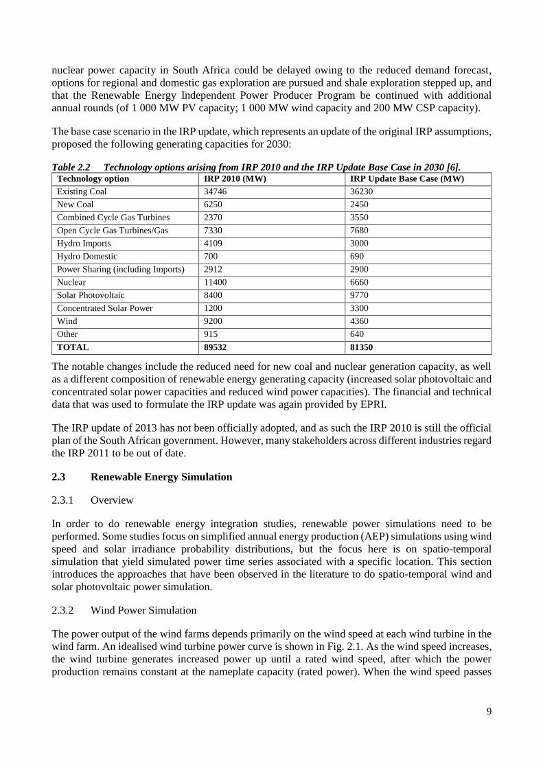
9

nuclear power capacity in South Africa could be delayed owing to the reduced demand forecast,

options for regional and domestic gas exploration are pursued and shale exploration stepped up, and

that the Renewable Energy Independent Power Producer Program be continued with additional

annual rounds (of 1 000 MW PV capacity; 1 000 MW wind capacity and 200 MW CSP capacity).

The base case scenario in the IRP update, which represents an update of the original IRP assumptions,

proposed the following generating capacities for 2030:

Table 2.2 Technology options arising from IRP 2010 and the IRP Update Base Case in 2030 [6]. Technology option IRP 2010 (MW) IRP Update Base Case (MW)

Existing Coal 34746 36230

New Coal 6250 2450

Combined Cycle Gas Turbines 2370 3550

Open Cycle Gas Turbines/Gas

Engines

7330 7680

Hydro Imports 4109 3000

Hydro Domestic 700 690

Power Sharing (including Imports) 2912 2900

Nuclear 11400 6660

Solar Photovoltaic 8400 9770

Concentrated Solar Power 1200 3300

Wind 9200 4360

Other 915 640

TOTAL 89532 81350

The notable changes include the reduced need for new coal and nuclear generation capacity, as well

as a different composition of renewable energy generating capacity (increased solar photovoltaic and

concentrated solar power capacities and reduced wind power capacities). The financial and technical

data that was used to formulate the IRP update was again provided by EPRI.

The IRP update of 2013 has not been officially adopted, and as such the IRP 2010 is still the official

plan of the South African government. However, many stakeholders across different industries regard

the IRP 2011 to be out of date.

2.3 Renewable Energy Simulation

2.3.1 Overview

In order to do renewable energy integration studies, renewable power simulations need to be

performed. Some studies focus on simplified annual energy production (AEP) simulations using wind

speed and solar irradiance probability distributions, but the focus here is on spatio-temporal

simulation that yield simulated power time series associated with a specific location. This section

introduces the approaches that have been observed in the literature to do spatio-temporal wind and

solar photovoltaic power simulation.

2.3.2 Wind Power Simulation

The power output of the wind farms depends primarily on the wind speed at each wind turbine in the

wind farm. An idealised wind turbine power curve is shown in Fig. 2.1. As the wind speed increases,

the wind turbine generates increased power up until a rated wind speed, after which the power

production remains constant at the nameplate capacity (rated power). When the wind speed passes

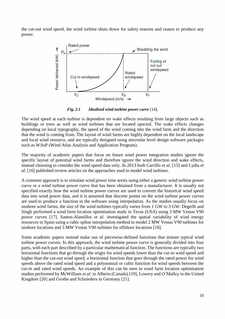
10

the cut-out wind speed, the wind turbine shuts down for safety reasons and ceases to produce any

power.

Fig. 2.1 Idealised wind turbine power curve [14].

The wind speed at each turbine is dependent on wake effects resulting from large objects such as

buildings or trees as well as wind turbines that are located upwind. The wake effects changes

depending on local typography, the speed of the wind coming into the wind farm and the direction

that the wind is coming from. The layout of wind farms are highly dependent on the local landscape

and local wind resource, and are typically designed using microsite level design software packages

such as WAsP (Wind Atlas Analysis and Application Program).

The majority of academic papers that focus on future wind power integration studies ignore the

specific layout of potential wind farms and therefore ignore the wind direction and wake effects,

instead choosing to consider the wind speed data only. In 2013 both Carrillo et al. [15] and Lydia et

al. [16] published review articles on the approaches used to model wind turbines.

A common approach is to simulate wind power time series using either a generic wind turbine power

curve or a wind turbine power curve that has been obtained from a manufacturer. It is usually not

specified exactly how the wind turbine power curves are used to convert the historical wind speed

data into wind power data, and it is assumed that discrete points on the wind turbine power curves

are used to produce a function in the software using interpolation. As the studies usually focus on

onshore wind farms, the size of the wind turbines typically varies from 1 GW to 3 GW. Degeilh and

Singh performed a wind farm location optimisation study in Texas (USA) using 3 MW Vestas V90

power curves [17]. Santos-Alamillos et al. investigated the spatial variability of wind energy

resources in Spain using a cubic spline interpolation method to model 2 MW Vestas V90 turbines for

onshore locations and 3 MW Vestas V90 turbines for offshore locations [18].

Some academic papers instead make use of piecewise-defined functions that imitate typical wind

turbine power curves. In this approach, the wind turbine power curve is generally divided into four

parts, with each part described by a particular mathematical function. The functions are typically two

horizontal functions that go through the origin for wind speeds lower than the cut-in wind speed and

higher than the cut-out wind speed, a horizontal function that goes through the rated power for wind

speeds above the rated wind speed and a polynomial or cubic function for wind speeds between the

cut-in and rated wind speeds. An example of this can be seen in wind farm location optimisation

studies performed by McWilliam et al. in Alberta (Canada) [19], Lowery and O’Malley in the United

Kingdom [20] and Grothe and Schnieders in Germany [21].

11

Ignoring the local typography and layout of a wind farm will necessarily have an impact on the

accuracy of the simulation. Another issue with wind power simulation is the spatial resolution of the

historical wind speed data. A multi turbine power curve methodology was developed by Nørgaard

and Holttinen to compensate for single historical wind speed time series that represent large

geographical areas [22]. The method involves several steps but essentially involves a convolution of

the Gaussian distribution with a chosen wind turbine power curve in order to approximate the

smoothing effect of distributing many turbines in a relatively small geographic area. The

methodology takes into account the size of the geographic area, the mean wind speed and the wind

turbulence intensity, and is shown to simulate historic wind power outputs more accurately than just

using a wind turbine power curve. A visual representation of the multi-turbine power curve is shown

in Fig. 2.2. An approach similar to that of Nørgaard and Holttinen was used by Reichenberg et al. to

investigate the variance dampening effect of optimising the geographic location of wind farm

locations [23].

Fig. 2.2 Visual Representation of the multi-turbine power curve approach [22].

A similar modelling method to that of Nørgaard and Holttinen was also used by Andresen et al. to

produce a renewable energy atlas for energy system analysis for Denmark [24], where historical wind

power production data was used to fine tune certain simulation parameters in order to improve

accuracy. The authors compared the multi-turbine power curve approach with the normal (single)

wind turbine power curve interpolation approach, and found that the multi-turbine power curve

approach showed better agreement with the actual wind turbine output data as can be seen in Fig. 2.3.

12

Fig. 2.3 Comparison of the single wind turbine power curve interpolation approach (left) and the

multi-turbine power curve approach (right) in the study by Andresen et al. [24], both plotted against

actual historical wind turbine outputs.

Other novel approaches to wind power simulation have also been proposed. Wood et al. developed a

stochastic model to produce synthetic time series of wind power at several locations based on a

measured time series of wind speed from a reference site [25]. Using a case study in south-eastern

Australia it was shown that, even though the local typography was ignored, the stochastic properties

of the modelled time series compared well measured data.

2.3.3 Solar Photovoltaic Power Simulation

The power output of the solar photovoltaic farms depends primarily on the solar irradiance that is

inclined on the solar photovoltaic panel, also referred to as the tilted irradiance, and the temperature

of the photovoltaic cell, although many other factors can influence the power output. Fig. 2.4. shows

the three irradiance components which make up the total inclined irradiance, namely the direct

irradiance, the diffuse irradiance and reflected irradiance [26]. The direct irradiance is the irradiance

that hits the panel on a direct path from the sun, the diffuse irradiance is the irradiance that has been

scattered by molecules and particles in the atmosphere and the reflected irradiance is the irradiance

that is reflected off other objects in the area surrounding the panel.

Fig. 2.4 The three components that make up to total inclined irradiance [26].

Mahela and Shaik published a review on grid interfaced solar photovoltaic systems [27], including

an overview of all the technical aspects involved in a solar photovoltaic system including the solar

cell, the PV array, maximum power point tracking, filters, DC-DC converters, inverters and control

techniques. These technical details will not be further investigated here as the interest is in a simple

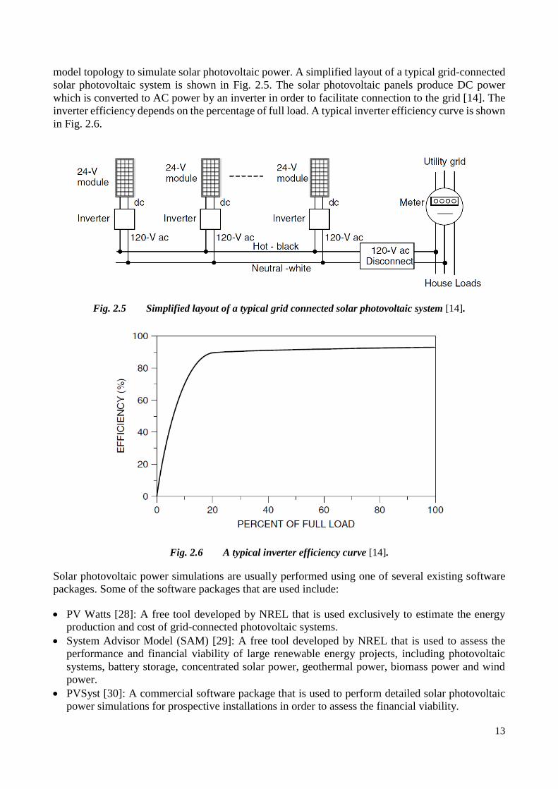
13

model topology to simulate solar photovoltaic power. A simplified layout of a typical grid-connected

solar photovoltaic system is shown in Fig. 2.5. The solar photovoltaic panels produce DC power

which is converted to AC power by an inverter in order to facilitate connection to the grid [14]. The

inverter efficiency depends on the percentage of full load. A typical inverter efficiency curve is shown

in Fig. 2.6.

Fig. 2.5 Simplified layout of a typical grid connected solar photovoltaic system [14].

Fig. 2.6 A typical inverter efficiency curve [14].

Solar photovoltaic power simulations are usually performed using one of several existing software

packages. Some of the software packages that are used include:

PV Watts [28]: A free tool developed by NREL that is used exclusively to estimate the energy

production and cost of grid-connected photovoltaic systems.

System Advisor Model (SAM) [29]: A free tool developed by NREL that is used to assess the

performance and financial viability of large renewable energy projects, including photovoltaic

systems, battery storage, concentrated solar power, geothermal power, biomass power and wind

power.

PVSyst [30]: A commercial software package that is used to perform detailed solar photovoltaic

power simulations for prospective installations in order to assess the financial viability.

14

2.4 Weather Datasets

2.4.1 Overview

In order to perform the wind power and solar photovoltaic power simulations described in section 2.3,

historical weather data with adequate time and spatial resolution are required. Depending on where

the in world these renewable power simulations are to be performed, this data might or might not be

available. This section introduces some major open source and proprietary databases that provide this

kind data.

2.4.2 Wind Datasets

There is a variety of wind data available in the world today. Wind data can generally be divided into

three categories based on the spatial resolution of the data, namely macroscale (50 km–200 km),

mesoscale (1 km–50 km) and microscale (10 m–100 m). Macroscale wind data is found in global

weather databases such as the Modern-Era Retrospective analysis for Research and Applications

(MERRA), a database of Nasa. These datasets are modelled and compiled using a variety of sources

including weather stations, aircraft and satellite instrumentation [20]. Mesoscale wind data, which is

usually modelled using macroscale wind data and other inputs, is typically used for large-scale wind

power integration studies. Microscale wind data is needed for wind turbine siting within a wind farm,

and is modelled using either measured wind data at a certain location or mesoscale wind data as well

as local typographical inputs.

Wind datasets, also called wind atlases, are datasets that provide statistical information on the wind

resource of a particular area on either a mesocale or microscale. Wind atlases generally provide wind

speed probability distributions, wind roses (diagrams showing the relative frequency of wind

directions) and wind resource maps that are constructed from the data, and most wind atlases

additionally provide wind speed and wind direction time series data at a certain time resolution,

usually at either 10 minute or hourly intervals.

Wind atlases can generally be divided into two categories based on how they were produced, namely

observational wind atlases and numerical wind atlases [31]. Observational wind atlases are created

using microscale modelling methods by incorporating measured time series data of wind speed and

direction, as well as characteristics of the local topography including elevation, roughness and

obstacles, which is usually obtained from satellite data. In the absence of long-term, high quality

measured wind data, a numerical wind atlas method is usually applied. Numerical wind atlas methods

use macroscale global weather datasets, such as the NCEP/NCAR global reanalysis data-set (National

Centers for Environmental Prediction and National Center for Atmospheric Research respectively),

as well as local typographical characteristics to produce mesoscale wind data that cover a large area,

usually an entire country. There are several numerical wind atlas methods, including the Karlsruhe

Atmospheric Mesoscale model (KAMM), the Weather, Research and Forecasting (WRF) model, the

High resolution Regional Model (HRM) and the High Resolution Limited Area Model (HIRLAM)

[32]. Mesoscale wind data from numerical wind atlases are often compared to observational wind

atlases for verification and validation purposes.

2.4.2.1 International Wind Atlases

There are many wind atlases available worldwide and the following review should by no means be

considered exhaustive. One of the first comprehensive wind atlases was the European wind atlas [33],

which was produced in 1989 by Risø National Laboratory. This wind atlas contained long-term wind

speed probability distributions, monthly mean wind speeds, mean cubed wind speeds and the average

15

daily wind speed pattern for every month. In addition, the spectral power density of the deviations

from the average monthly daily pattern was also presented. The statistics were constructed using

measured data from 220 meteorological stations as an input to the WAsP computer program. The data

from the European wind atlas was used by Beyer and Nottebaum [34] to synthesise hourly wind speed

time series in 1995.

An observational wind atlas and numerical wind atlas was created for Egypt in 2006 [35] with a

spatial resolution of 7.5 km. The numerical wind atlas, which utilised the KAMM mesocale model,

covered the entire land area of Egypt, while the observational wind atlas covered the areas

surrounding 30 meteorological stations.

A wind atlas for the Iberian peninsula was presented by Gastón et al. in 2008 [36] using the Skiron

mesoscale model for the wind speed in 2006 on a 0.1° spatial resolution. The wind map that was

produced was validated using measured wind data from 50 meteorological stations.

A wind atlas was created for Greece in 2006, and updated in 2008, using measured wind data from

around 200 measurement stations. Kotroni et al [37] produced a complimentary wind atlas for Greece

in 2013 using the MM5 numerical wind atlas method for a typical wind year at 10-minute time

resolution and 2 km spatial resolution. The typical wind year was constructed using data from certain

months over a 20 year period using the method proposed by Hall et al [38].

In 2008, a Finnish wind atlas was produced using the HIRLAM and AROME (Application of

Research to Operations at MEsoscale) mesoscale models [39]. This wind atlas replaced the Finnish

wind atlas of 1991. A spatial resolution of 2.5 km was employed, but in areas with the most favourable

characteristics for wind power production, the output of the mesocale model was used as an input to

a diagnostic downscaling method with WAsP to create wind data with a higher spatial resolution of

250 m. A 48-month reference period was constructed for the mesoscale simulation from data that

represents 1989 until 2007.

In 2015 the National Renewable Energy Laboratory (NREL) and Vaisala collaborated to produce the

Wind Integration National Dataset (WIND) Toolkit that is meant to support wind power integration

studies in the United States [40], expanding upon the Western Wind and Solar Integration Study

(WWSIS) data set that was created in 2008. The WIND Toolkit presents meteorological data

(including wind speed) produced by the WRF method, with a 5-minute time resolution and 2 km

spatial resolution for more than 126 000 sites that have been identified as potential future locations

for wind farms. The data spans the period from 2007 until 2013, and also includes the wind power

production time series produced using site-specific wind turbine classes and simulated power

forecasts that have been produced to mimic the power forecast methods used in industry.

2.4.2.2 Wind Atlas of South Africa

The Wind Atlas of South Africa (WASA) project was started in 2009 by the South African

government and several industry and academic partners including the South African National Energy

Research Institute (SANERI), the Council for Scientific and Industrial Research (CSIR), the

University of Cape Town (UCT), the South African Weather Service (SAWS), Risø National

Laboratory and Technical University of Denmark (DTU). The project aimed to produce both an

observational and numerical wind atlas for South Africa, with the former being used to validate the

results of the latter. The project would cover a large region spanning across the Northern Cape,

Western Cape and Eastern Cape, as this represented the area where most of the wind farms in South

Africa were projected to be built.

16

For the observational wind atlas, 10 masts were erected at selected sites throughout South Africa to

record wind speeds at different heights, as well as other meteorological data. The location of the masts

can be seen in Fig. 2.7

Fig. 2.7 Locations of the 10 meteorological masts in the WASA project [41].

Two numerical wind atlases have been produced in the WASA project. The first numerical wind atlas

was produced using the KAMM-WAsP method in 2012, resulting in 15 000 data points on a

5 km x 5 km spatial resolution. The second numerical wind atlas was produced in 2014 using the

WRF method, resulting in 40000 data points on a 3 km x 3 km spatial resolution. Each of these data

points are available for download by the public as .lib files, which can be used as an input in the

WAsP program to do wind turbine micrositing within wind farms. It was found that the KAMM-

WAsP method slightly underestimated the wind resource when compared to observational wind atlas,

with a mean bias and mean absolute bias of −8.2% and 9.3% respectively. The WRF method

performed better, showing an average under or overestimation of 4.7% across all sites [31]. Overall,

the WRF method overestimated the wind resource by 2.5%. A map of the mean wind speeds across

the project area can be seen in Fig. 2.8.

17

Fig. 2.8 Mean Wind Speed Map produced by the WRF method in the WASA project [9].

The WASA project also availed itself of time series data, which was produced using the WRF method,

with a spatial resolution of 27 km x 31 km resulting in 527 time series covering the project area. The

time series data comprised hourly wind speed at 100 m and wind direction for the period 01-09-1990

to 31-12-2012.

2.4.3 Solar Datasets

In order to perform solar photovoltaic power simulations, a minimum requirement is historical solar

irradiance data and temperature data. Temperature data is usually sourced from national weather

services, while solar irradiance data can be obtained from weather stations or calculated from

meteorological satellite data. There are many free sources of solar irradiance data, although high

quality data normally comes in the form of proprietary data sources such as SolarGIS [42] or SODA

[43].

In 2014, SolarGIS developed maps that showed the annual solar irradiance levels in South Africa.

Fig. 2.9 shows annual sums of global horizontal irradiance for South Africa.

18

Fig. 2.9 Map of global horizontal irradiance in South Africa by SolarGIS [44].

2.5 Renewable Energy Integration Studies

2.5.1 Overview

There exists a vast amount of literature on renewable energy integration studies. This section

introduces two topics that are under consideration in this study. The first is the key performance

indicators that are related to increased renewable energy penetration. This topic deals with the ways

in which the impact of increasing renewable energy sources on the power system is quantified. The

second topic deals with the ratio of wind farm capacity to solar photovoltaic capacity. These two

sources represent the main technologies that are under consideration for large scale integration, yet

they deliver very different power profiles, which complement the load profile of each country in a

different way. Several studies exist that try to determine the optimal ratio of wind power to solar

power by considering different optimisation targets. A critical aspect of wind and solar power

19

integration studies that is not considered in this overview, is the need for increased operating reserves,

of which a comprehensive review was published by Holttinen et al. [45] in 2012.

2.5.2 Key Performance Indicators Related to Increased Renewable Energy Penetration

When a new power plant is added to a power system, its impact on the reliability of the power system

is of interest. The reliability of a power system is divided into two parts, namely power system

security and power system adequacy [46]. Power system security deals with the ability of a power

system to maintain steady power delivery in the event of a critical failure of one of the power system

components such as a large power station or a critical transmission line. Power system adequacy deals

with the ability of a power system to meet the load demand at any given time, i.e. having enough

installed capacity with sufficient reserve, considering all the factors that influence the ability of

different technologies to deliver power when it is needed.

2.5.2.1 Power System Security

In terms of power system security, it is broadly understood that renewable energy sources such as

wind power and solar power contributes positively to the ability of a power system to absorb critical

failures at any given time [47]. The reason for this is twofold. First, both these renewable energy

sources are distributed, reducing their dependence on any one transmission link or node. Secondly,

the sizes of the generators are considerably smaller than that of conventional generators, meaning that

the failure of a typical wind turbine or solar panel is much less significant than that of a coal, gas or

nuclear generator. There is concern around the impact of cloud cover moving over solar photovoltaic

plants, which could result in a very sudden interruption of power flow from that plant. Jewell and

Ramakumar [48] used solar power simulations to quantify the time that it would take, in a worst case

scenario, for a solar photovoltaic power system to go from full power production to zero power

production when a squall line of cloud cover moves across an otherwise clear sky. They found that

in the case where the solar photovoltaic power system is spread across 10 km2, the time for complete

power loss is 1.8 minutes. In the case where the solar photovoltaic power system is spread across

1 000 km2 and 100 000 km2, the time for complete power loss increases to 17.6 minutes and

175.7 minutes respectively. Rowlands et al. [49] performed a study on solar photovoltaic power

dispersion in Ontario, Canada, which found that increasing reductions in solar photovoltaic power

variability could be achieved by dispersing solar photovoltaic plants up to 800 km away from each

other, after which the reductions in variability become insignificant. Shivashankar et al. [50]

published a comprehensive review on the methods that are used to mitigate the power fluctuation of

solar photovoltaic systems. The methods include geographical dispersion, different energy storage

technologies and backup diesel generators. Although graphical dispersion is found to reduce the

variability of wind power output, the paper concludes that the use of storage technologies will become

indispensable at high penetrations of solar photovoltaic power. The review also mentioned the

methods that are used to do solar photovoltaic power forecasts, with artificial neural networks

currently outperforming other methods.

2.5.2.2 Power System Adequacy

There are several measures that are used when accessing power system adequacy. These include the

loss of load expectation (LOLE) and the loss of load probability (LOLP). The LOLP is the probability

that the full load demand will not be met at a given point in time:

( )Ti i iLOLP p L C (2.1)

20

where 𝑝() indicates probability, 𝐿𝑖𝑇 is the total load at time 𝑖 and 𝐶𝑖 is the available generation

capacity at time 𝑖.

The loss of load expectation (LOLE) is the number of hours during a given timeframe, usually

specified as a year, that the load will not be met:

1

T

ii

LOLE LOLP

(2.2)

The LOLE is usually calculated by means of a capacity outage probability table (COPT), which

represents the different capacity outage levels and their associated probabilities [51]. A COPT is

constructed by convolving the capacities and forced outage rates (FOR) of the conventional

generation plants. Convolution of the COPT and the load duration curve results in the LOLE. In the

absence of detailed generation plant data, the targeted loss of load expectation (LOLE) is often chosen

as 0.1 days/year.

It is difficult to model renewable energy sources in the traditional way using FORs, because their

ability to deliver power relies heavily on the weather and not so much on mechanical availability.

Conventional generation units can be modelled as 2-state distributions (available or unavailable),

whereas renewable energy sources produce a range of different power output levels that depends on

the weather. Therefore, in terms of power system adequacy, different penetrations of renewable

energy sources result in broadly two different types of studies. At low to medium penetrations of

renewable energy sources, a certain amount of conventional generating capacity can effectively be

displaced (or in the case of increasing annual load demand, conventional generating capacity

expansion can be avoided). In this case, the capacity value and capacity credit are examined, and is

further discussed below in section 2.5.2.3. Studies that consider high penetrations, where the capacity

credit of renewable energy sources become very low, focus rather on the backup generating or storage

needs that will be necessary to maintain the power system adequacy. Studies of this nature are

described in section 2.5.2.4.

2.5.2.3 Capacity Credit of Renewable Power Plants

There have been a lot of publications that deal with the capacity value and capacity credit of

renewable energy plants, resulting in many different proposed methods to determine these values. To

provide a complete overview of all the publications regarding the capacity value and capacity credit

of renewable energy sources is beyond the scope of this thesis, and as such the discussion is limited

to three publications that have often been cited in the literature. The three publications focus on the

methods used to determine the capacity value of conventional units, wind farms and solar

photovoltaic farms. We also include one study that performed an in-depth investigation of factors that

influence the capacity value calculation of wind farms when using the preferred method from one of

the above-mentioned publications.

The capacity value is broadly defined as the amount of additional load that can be served due to the

addition of the generator, while maintaining the existing levels of reliability [46]. Capacity credit is

simply the capacity value associated with a specific generator, divided by the total power capacity of

that generator, as shown here:

capacity value

capacity creditnameplate capacity

(2.3)

21

Amelin [52] published a study in 2009 where four methods of determining the capacity credit of

conventional power plants were compared. The four methods are:

the equivalent firm capacity method

the effective-load carrying method

the equivalent conventional power plant method

the guaranteed capacity method.

Each method determines a capacity (usually in MW) associated with a new power plant added to a

system that is analogous to the capacity value. In the first three methods, the load demand is taken

into account and the methods are all concerned with how the new unit affects the LOLP of the system.

In this study the LOLP is calculated using a duration curve that is used to represent the probability

distribution of the equivalent load. The duration curve is determined by the Baleriaux-Booth [53]

formula. The mathematical details of all the methods can be found in the study [52]. The equivalent

firm capacity is defined as the size of a fictitious power plant with a 100% availability that brings

about the same decrease in LOLP as the actual added power plant (which will necessarily have an

availability of less than 100%). The effective-load carrying method, which was first proposed by

Garver [54], determines the largest constant load that can be added to a system due to the addition of

the new power plants, without increasing the LOLP. The equivalent conventional power plant method

is similar to the firm capacity method, but instead specifies that the fictitious power plant, that will

reduce the LOLP by the same amount as the actual added power plant, has a reference availability

that is usually specified as 95%. The guaranteed capacity method determines the least capacity which

can be expected to be available with a given probability. All four methods were applied to 1000 MW

conventional power plant with a FOR of 10%, that is added to test systems with different levels of

installed capacity, mean load levels, load variances and availabilities of the existing capacities. All in

all there existed 135 different test systems. The existing capacity ranged from 15 GW to 30 GW, the

mean load levels ranged from 60% to 73% of installed capacity (the loads were all normally

distributed), the load variances ranged from 8% to 12% of mean load and the existing plants

availabilities ranged from 90% to 94%. All four methods were also applied to 2800 MW of wind

power capacity that has a probability distribution that is based on actual data from Sweden. The size

of the wind power capacity was chosen so that it has roughly the same energy production over a given

timeframe as the 1000 MW of the capacity of a conventional power plant. The results from the case

study showed that the method used to calculate the capacity credit can have a significant impact. The

equivalent firm capacity method and the effective-load carrying method displayed similar results,

while the equivalent conventional power plant method depends on an arbitrarily chosen availability,

but shows the same trends as the first two methods. Expectedly, the guaranteed capacity method,

which was the only method that does not incorporate the load demand, did not correlate well with the

other methods. Another clear trend was that in both the case of the conventional plant addition and

the wind power capacity addition, the capacity credit tended to be higher when added to systems with

high LOLP, i.e. the added capacity contributed more to lowering the LOLP. The capacity credit

decreased with the penetration level of the added capacity. As expected, the capacity credit for the

added wind power capacity was lower than what it was for the added conventional power capacity.

The author concludes by suggesting that either the equivalent firm capacity or equivalent load

carrying capacity methods be used.

In 2008, the Wind Power Coordination Committee and Power Systems Analysis, Computing and

Economics committee of the IEEE Power and Energy Society (PES) set up a task force to provide

clarity on the issue of capacity credit of wind power capacity. The taskforce’s meeting resulted in the

publication by Keane et al. [46] in 2011, which put forth a preferred method for the calculation of

22

wind farm capacity while also reviewing some of the popular approximation methods. The preferred

LOLE method consists of three steps:

In the first step, the LOLE is calculated for a system by considering the load time series and the

COPT of the conventional generators as described in section 2.5.2.2.

In the second step, the wind power output time series of the wind capacity in question is subtracted

from the load time series, and the resulting residual load time series is used to calculate a new

LOLE as in the first step. The new LOLE will necessarily be lower than the LOLE in the case with

no wind power.

In the last step, a constant load is added iteratively to the residual load time series until the LOLE

equals the LOLE that was calculated in the first step.

To be clear, the residual load time series in step 2 above is formulised as

1

NR T xi i i

x

L L W

(2.4)

where 𝐿𝑖𝑅 is the residual load at time 𝑖, 𝐿𝑖

𝑇 is the total load at time 𝑖, 𝑁 is the number of wind farms,

𝑊𝑖𝑥 is the wind power output at wind farm 𝑥 at time 𝑖.

The authors highlight that this method is based on the original definition of capacity value, i.e. the

amount of additional load that can be served due to the addition of a certain wind power capacity

(while maintaining the same reliability). The main strength of this method is that is captures the

correlation between the wind power output and the load time series. The authors also emphasise that

any capacity value calculation is only as reliable as its input data. Due to the significant inter-annual

variation, it is stated that using data for one year is not adequate. The data that is required for this

preferred method are the following [46]:

multi-year load time series of at least an hourly time resolution

wind power output time series that exactly overlaps with the load time series

complete inventory of the capacity, forced outage rates and maintenance schedules of the

conventional generation units.

As this data is not always available, there exist several capacity value approximation methods. The

review of the capacity value approximation methods in this publication draw from the work done by

Dent et al. [55], and the methods include the Garver approximation based method, multi-state unit

representation, annual peak calculations and the Z-statistic method. Another approximation method

is the peak-period capacity factors method, but the authors indicate that this method should be used

as a quick screening method rather than a formal capacity value approximation method because it

captures neither the variability of wind power nor the correlation between wind power and load.

The Garver approximation based method stems from a graphical method to calculate the effective

load carrying capability (ELCC) of a generator that was introduced by Garver in 1966 [54]. The

Garver approximation based method is convenient because it only requires the load time series and

the wind power time series. The Garver capacity value approximation makes the assumption that

𝐿𝑂𝐿𝑃 ∝ 𝑒(

𝐿𝑇

𝑚), and calculates the capacity value, 𝑎, as follows [56]:

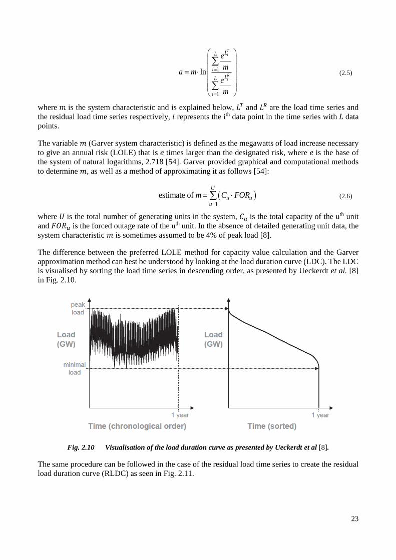
23

1

1

ln

Ti

Ri

LL

i

LL

i

e

ma m

e

m

(2.5)

where 𝑚 is the system characteristic and is explained below, 𝐿𝑇 and 𝐿𝑅 are the load time series and

the residual load time series respectively, 𝑖 represents the ith data point in the time series with 𝐿 data

points.

The variable 𝑚 (Garver system characteristic) is defined as the megawatts of load increase necessary

to give an annual risk (LOLE) that is 𝑒 times larger than the designated risk, where 𝑒 is the base of

the system of natural logarithms, 2.718 [54]. Garver provided graphical and computational methods

to determine 𝑚, as well as a method of approximating it as follows [54]:

1

estimate of U

u uu

m C FOR

(2.6)

where 𝑈 is the total number of generating units in the system, 𝐶𝑢 is the total capacity of the uth unit

and 𝐹𝑂𝑅𝑢 is the forced outage rate of the uth unit. In the absence of detailed generating unit data, the

system characteristic 𝑚 is sometimes assumed to be 4% of peak load [8].

The difference between the preferred LOLE method for capacity value calculation and the Garver

approximation method can best be understood by looking at the load duration curve (LDC). The LDC

is visualised by sorting the load time series in descending order, as presented by Ueckerdt et al. [8]

in Fig. 2.10.

Fig. 2.10 Visualisation of the load duration curve as presented by Ueckerdt et al [8].

The same procedure can be followed in the case of the residual load time series to create the residual

load duration curve (RLDC) as seen in Fig. 2.11.

24

Fig. 2.11 Visualisation of the residual load duration curve as presented by Ueckerdt et al [8].

The preferred LOLE method for capacity value calculation uses a LOLE that is calculated using the

FORs of the conventional generating units. This LOLE, which is typically around 0.1 days per year,

specifies the single points on the LDC and the RLDC that are considered, close the top left of the

graphs in Fig. 2.10 and Fig. 2.11 where the x-axis is for example 2.4 8760⁄ of the length of the time

series. In the Garver approximation based method, where the LOLE is not known, the entire load time

series and residual load time series are taken into account, but because the ratio of exponentials is

implicit in equation (2.5), the peak load and residual load values to the top left contribute much more

than the rest of the respective time series.

If a complete wind power time series that is time synchronous with the load data, is unavailable, the

Garver approximation based method can still be used by employing the multi-state unit representation

method, where the wind power output is modelled as a power unit that has multiple levels of power

output with associated probabilities (ranging between 0 and full rated power). In this case, the

capacity value, 𝑎, reduces to [57]:

1

ln x

Xmw

xx

a p em

(2.7)

where 𝑋 is the number of different states that the wind power output can take, 𝑝𝑥 is the probability

that the wind power output is 𝑤𝑥.

The multi-state unit representation method can also be used on its own, without the Garver

approximation. The LOLE is then calculated in the traditional way using the COPT as described in

section 2.5.2.2, modelling the conventional generating units as dual state (either available or not) and

the wind power units as multi-state. The main weakness of the multi-state representation method is

that the correlation between load and wind power output is lost. This can be compensated for by using

different probability distributions for different hours of the day, or by employing Markov models for

different states of wind power output. However, the effect that certain weather conditions will have

on the load is difficult to capture using this methodology.

25

Dent et al. [55] performed a case study in Great Britain, where the peak demand and LOLE are 60 GW

and 0.061 hour/year respectively, and found that the Garver approximation based method with multi-

state unit representation provided a good approximation, only overestimating the capacity credit at

low penetrations when compared to the preferred LOLE method, as can be seen in Fig. 2.12. The

three different lines of the Garver approximation based method with multi-state unit representation

(90%, 95%, 97%) represents three different cases where the wind power output probability during

10%, 5% and 3% of peak load demand were considered.

Fig. 2.12 Comparison of preferred LOLE capacity value calculation with the Garver approximation

method with multi-state unit representation, for a case study in Great Britain [55].

Annual peak calculations can be performed using multi-state unit representation, by considering only

the LOLP at the time of annual peak load. Thus, probability distributions are needed for the peak load

and the wind power output during the specific time of year. This measure is used as a proxy for system

risk in some countries [46]. Because the peak load only occurs once a year and not necessarily in the

exact same time of year, obtaining accurate probability distributions for wind power output is seen as

a major hurdle. Several approaches have been followed to mitigate this limitation, including the use

of the entire peak season or using a subset of days that imitate the peak load day.

The Z-statistic method, the final capacity value approximation method considered by Keane et

al. [46], was proposed by Dragoon and Dvortsov [58] in 2006. In this method, the difference between

the available resources and the peak load demand, referred to as surplus of available generation, is

assumed to have a normal distribution and its mean is given by [58]:

S R L (2.8)

where 𝑆 is the mean surplus during peak hours, 𝑅 is the mean resources available during peak load

hours and 𝐿 is the mean peak load. As per the central limit theorem, as the system becomes larger,

i.e. as it consists of a larger amount of generating units, the probability distribution of the surplus

available generation will approach the normal distribution. The probability distribution of 𝑆 is shown

in Fig. 2.13.

26

Fig. 2.13 Probability Distribution of Surplus Generation [58].

The paper recognises that the surplus of available generation is a random variable and that the ratio

of the expected (mean) surplus to the standard deviation of the surplus is an indication of resource

adequacy, as given by the Z-statistic [58]:

s

SZ

(2.9)

where 𝜎𝑠 is the standard deviation of the surplus available generation about the mean. As indicated

on Fig. 2.13, the LOLP probability is calculated as the area of the probability distribution that falls to

the left of zero, i.e. when the load exceeds the available generating capacity. It follows that systems

with higher Z-statistics will have lower LOLPs. When additional generating capacity, such as wind

power capacity, is added to the system, the Z-statistic will increase. In this case, the amount of load

that can be added to the system, while keeping the Z-statistic constant (maintaining a constant LOLP),

is defined as the effective load carrying capability and provides the approximation for the capacity

value of wind power. More formally, the capacity value, 𝑎, is approximated as [58]

0 w

s

Za

(2.10)

where 𝜇 is the mean wind power output, 𝑍0 is the Z-statistic before the addition of wind power and

𝜎𝑤 is the standard deviation of the wind power output. There are two assumptions in this method.

When adding wind power output, which typically does not have a normally distributed power

output, the shape of the surplus available generation does not change significantly (although the

mean and standard deviation might change).

The standard deviation of the wind power output, 𝜎𝑤, is smaller than the standard deviation of the

surplus available generation, 𝜎𝑠.

Both these assumptions only hold true for low penetrations of wind power. Indeed, in the case study

by Dent et al. [55] of Great Britain that was mentioned above, the results of the Z-statistic method

started deviating from the preferred LOLE method for higher penetrations of wind power, as can be

seen in Fig. 2.14 (here the preferred LOLE method is indicated as “COPT”, while “Normal” indicates

a method that is similar to the preferred method with the addition that the conventional generating

27

fleet availability is modelled as a normal distribution instead of using the FORs of individual unitsto

compute a COPT).

Fig. 2.14 Comparison of preferred LOLE capacity value calculation (marked as “COPT”) with the Z-

statistic method approximation for capacity value for a case study in Great Britain [55].

In 2016, Nguyen et al. [59] published a study on the factors that influence the capacity value of wind

power. The method used to calculate the capacity value in this study is the preferred LOLE calculation

method from Keane et al. [46]. As discussed above, the traditional factors include FORs of

conventional power stations, system reliability targets, and the correlation between wind power

output and system load which is captured by the residual load. This in depth investigation, which

used the Australian National Electricity Market power system as a case study, examined the effects

of the number of wind farms and wind installed capacity, as well as the length of historic time series

data on demand and wind resources. The study concluded that subjective factors regarding wind

power simulation can affect the capacity value estimates and highlighted the importance of capturing

extreme risk events in the data, such as periods of extremely high temperatures which could result in

high levels of demand. In the case of the Australian National Electricity Market, it was found that

extreme load events occurred for about nine days in the fifteen year dataset. Including these extreme

load events reduced the capacity credit from about 12–15% to about 7–9%. The fact that capacity

value calculations showed significant variance in this one study, even when using the preferred

calculation method, caused the authors to suggest that capacity value estimates should not be regarded

as definite contribution values, but rather as indicative figures that aid policy making and investment

decisions for electrical power systems.

Madaeni et al. [56] published a study in 2013 on the capacity value estimation techniques for solar

photovoltaic power. They compared traditional methods, including effective load carrying capability

and equivalent conventional power, with several of the above-mentioned capacity value

approximation methods including a weighted capacity factor-based approximation, the Garver

approximation based method, the Garver approximation based method with multi-state generators

and the Z-statistic method. A case study was performed for 14 sites in the Western Electricity

Coordinating Council (WECC) region in the United States with hourly data from 1998 to 2005. The

capacity value of 100 MW-DC (translating to 83.4 MW-AC under standard test conditions) of solar

photovoltaic capacity was considered for each site in isolation, and as such the authors emphasise

that this is a study on the marginal addition of solar photovoltaic power that does not take into account

the decreasing capacity values that are associated with large penetrations of solar photovoltaic power.

The solar photovoltaic power time series were modelled using the Solar Advisor Model (SAM) of

the National Renewable Energy Laboratory. The results show that solar photovoltaic power has a

28

lower effective load carrying capability than an equivalent conventional power rating, due to the fact

that computing the effective load carrying capability involves iterative addition of a constant load,

essentially comparing the solar photovoltaic power with a fully reliable generator. It is therefore

expected that this value will be lower than the equivalent conventional power rating, where a non-

zero FOR is assumed. Using the root-mean-square error (RMSE) between the results of the

approximation methods and the capacity value as calculated using the effective load-carrying

capability method, it is shown that the weighted capacity factor based method provides the best

estimate, although all methods showed a RMSE of less than 10%. The paper also emphasises the

cases where capacity values of solar power might be high despite relatively low capacity factors, due

to the correlation of solar power with the regional load.

2.5.2.4 Effect of Increasing Share of Renewable Energy on Conventional Generation Type

At larger penetrations of renewable energy, the total capacity credit of the total renewable energy

portfolio becomes very low, and the focus in such instances shifts to the storage needs and the type

of conventional (dispatchable) generating capacity that will be needed to supply the load. The bulk

of today’s load is supplied by base-load generating plants using coal, gas and nuclear technologies.

The majority of these plants were not designed to ramp up and down on daily or hourly time scales.

With a high penetration of variable renewable energy in the power system, the demand for base-load

generating will be less, whereas demand for load-following plants and peaking plants will likely

increase in addition to the integration of more energy storage capacity and demand side management

(DSM) strategies. Relatively few broad studies exist on the type of generating plants that will be

needed in the future as the exact generating fleet makeup needed to supplement the renewable energy

sources of a region is very specific to the system and physical grid layout. Two such broad studies

are presented here, each with their own methodologies to determine the sizes of conventional

generation of different flexibility classes. These methodologies are not meant to prescribe the exact

makeup, but rather to provide insight into the changing generating needs as the penetration of

renewable energy sources increase.

Tarroja et al. [60] published a study on the different metrics that can be used to measure the impact

of renewable energy on utility load-balancing, using primarily the characteristics of the residual load

time series (referred to as the “net load signal”). The characteristics of the net load signal that were

considered include parameters such as the maximum, minimum, range and capacity factor, as well as

metrics such as the surplus renewable fraction, load duration curve, daily occurrences of

maximum/minimum values, generator duration counts and power spectral density. The generator

duration counts metric, also referred to as the generator capacity by type metric, is investigated further

in this overview. The generator duration counts metric is a novel high-level statistical method that is

proposed to estimate the size of balance generator types (peaker, load-following or base-load) that

will be required to meet the load. This metric is calculated using only the net load signal and ignores

other elements such as the spinning reserve requirements or demand side management.

Each of three types of generators, namely base-load, load-following and peaker plants are assigned a

duration period length, which represents the typical average time that the specific type of generator

will be online. The duration period lengths are given in Table 2.3. These duration period lengths are

based on an examination of actual generator dispatch from Federal Energy Regulatory Commission

in the year 2000 for the state of California.

29

Table 2.3 Generator Type Duration Period Lengths [60]. Generator Type Duration Period Length Typical generator types

Peaker ≤5 h Natural-gas brayton cycle

Reciprocating engines

Load-following 6-168 h Natural-gas combined cycle

Natural-gas rankine cycle

Natural-gas brayton cycle

Base-load 169+ h Nuclear rankine cycle

Coal-powered rankine cycle

Gasified coal-powered combined cycle

Next, the base-load, load-following and peaker plant totals are initialised as 0 MW. Generator

duration lengths are obtained by examining the net load signal at different power levels which are

increased by equal increments, Pinc, from zero. Pinc is arbitrarily specified as 10 MW in this study. At

each power level, the periods of generator operation at or above that power level are located and each

of their durations recorded. A graphical representation of this process is presented in Fig. 2.15. The

generator duration lengths (t1, t2, t3, …) are grouped according to duration period lengths of the

different types of generators. Pinc is then divided into three parts in the same proportion as the

generator duration length groupings and added to the base-load, load-following and peaker plant

totals.

Fig. 2.15 Visualisation of the generator duration counts metric by Tarroja et al. [60].

For example, if at 33 GW, zero of the generator duration lengths are longer than 168 hours, two thirds

of the generator duration lengths are between 6 hours and 168 hours and the remaining third of the

generator duration lengths are less than 6 hours, 0 MW will be added to the base-load total, 6.66 MW

will be added to the load-following total and 3.33 MW will be added to the peaker total. In effect this

means that the marginal demand at between 33 GW and 33.01 MW will be served by load-following

plants 66.6% of the time and by peaker plants 33.3% of the time. After this process is repeated for

successive power levels up until the maximum value of the net load signal, the totals for the different

types of generators are obtained.

It is emphasised that this method ignores the actual dispatch scenarios that stem from market

operations in regional balancing entities, and that it is intended to provide a rough estimation of

typical generator dispatch by type [60]. This method also assumes that there is no uninterruptable

base load, and that renewable energy curtailment will only occur in cases where the load is smaller

30

than the total renewable power, i.e. where the net load signal is negative. In some real world scenarios,

it might be more economical to keep base-load stations online and curtail renewable energy sources

during low residual demand periods. The authors also emphasise that this method estimates the

capacity of different generator types to meet the load, and not the energy obtained from each type,

i.e. the capacity factors of each type.

A case study is performed that considered increasing penetrations of wind and solar photovoltaic

power, along with a small percentage of hydro, biomass, biogas, and geothermal power in California

in the United States [60]. The assumed proportions of the different technologies, which vary by

penetration level, are adapted from different sources and can be seen in Fig. 2.16.

Fig. 2.16 Projected technology proportions in the increasing penetration of renewable energy in the

California case study by Tarroja et al. [60].

Using the assumed technology proportions and hourly weather data, the combined renewable energy

time series of different penetrations of renewable energy were simulated, ranging from 13% to 75%.

These simulated time series are then used in conjunction with load data for the entire state of

California to calculate the generator capacity by type metric, which can be seen in Fig. 2.17. It is clear

that as renewable energy penetrations increase, the base-load generation total decreases while the

load following total remains fairly constant. The peaking generation total also remains fairly constant

up until around 40% penetration of renewables, after which it gradually increases, mainly due to the

increased reliance on variable wind and solar photovoltaic power. The authors note that increasing

solar power capacity tends to displaces base-load capacity with peaking power capacity, while

increasing wind power capacity tends to replace base-load capacity with load-following capacity.

However, the interaction between the wind and solar photovoltaic power cause the increasing load-

following capacity requirements from wind power also to be displaced by peaking power capacity.

31

Fig. 2.17 Results of the generator capacity by type metric for the California case study by Tarroja et

al. [60].

Schlachtberger et al. [61] performed a study on the need for dispatchable generating capacity from

different flexibility classes when power systems transform from low to high shares of variable

renewable power generation. The flexibility classes try to capture the different timescales of

renewable energy variability that are linked to the associated weather patterns, namely diurnal (intra-

day), synoptic (intra-week), and seasonal timescales. The study assumes that all residual load will be

covered by three sources that represent the aggregated contribution of all generating units in the

respective flexibility class. The dispatch of each of the three sources is determined using an

optimisation procedure that minimises the excess and deficit of backup energy with small installed

capacities and high utilisation. The objective function incorporates terms and variables that dictate

the order in which the three systems are dispatched. Two of the three flexibility classes are each

assigned a maximum ramp rate by considering the current load time series, i.e. the load time series

without significant shares of renewable energy in the system. In order to determine the maximum

ramp rate in each of the two cases, the current load time series is smoothed using convolution with a

Gaussian kernel. In the case of the slowest flexibility class, the Gaussian kernel has a standard

deviation of one week, whereas in the case of the medium flexibility class it has a standard deviation

of one day. After the smoothing procedure the signal is differentiated, and the maximum ramp rate

of the each flexibility class is assigned as the maximum of the differentiated, smoothed signal. As the

fastest flexibility class is assumed to be able to meet the load at all times, its ramp rate is left

unconstrained. More details on the methodology can be found in the publication.

The study considers eight years of hourly weather and load data in Germany and Europe as a whole,

and assumes that any added renewable energy capacity is made up of 70% wind power capacity and

30% solar photovoltaic power capacity. The result of the dispatch procedure for Germany can be seen

in Fig. 2.18, where the dispatch of the three sources in the case of 0%, 50% and 100% renewable

energy penetration are shown for a two-week period in October 2000. Note that penetration is defined

as the ratio of the capacity factor of the renewable energy to the mean load.

32

Fig. 2.18 Example of the dispatch result of the three flexibility classes (normalised to mean load) in the

case of different renewable energy penetrations in the study by Schlachtberger et al. [61].

The dispatch result is analysed and the maximum capacities for each of the three flexibility classes

are captured. The total capacities needed in the three flexibility classes are shown in Fig. 2.19. It is

clear that the need for the slowest flexibility class (seasonal) reduces while the share of renewables

increases, while the medium flexibility class initially increases up to about a 40% or 50% share of

renewables after which it decreases. It is also clear that there are major advantages to integrating the

European power system, as the total backup generating capacity reduces from 120% of mean load in

the case of Germany alone, to about 90% of mean load in the aggregated European case. This trend

continues for higher shares of renewables.

Fig. 2.19 Capacities of the different flexibility classes (normalised to mean load) needed to supplement

different shares of renewable energy in Germany (DE) and Europe (AGG) in the study by

Schlachtberger et al. [61].

2.5.3 Ratios of Wind Farm Capacity to Solar Photovoltaic Farm Capacity

Many publications exist in the literature that study the optimal ratio of wind power capacity to solar

photovoltaic power capacity by considering different simulation and optimisation strategies. The

majority of these studies consider large penetrations of renewable energy, typically 20% penetration

to 100% penetration and more. Unless stated otherwise, penetration level is defined as the mean

power output of the respective renewable technology divided by the mean load.

33

2.5.3.1 Minimisation of Curtailed Wind and Solar Photovoltaic Energy in New York State

Nikolakakis and Fthenakis [62] performed a study in 2011 on the optimal ratio of wind power

capacity to solar photovoltaic capacity in the state of New York in the United States. The authors

define a grid flexibility variable, where the minimum level that the conventional generating fleet can

ramp down to is stated as a percentage of annual peak load, and the grid flexibility is defined as 100%

minus the minimum ramp-down level. For example, if the peak load is 30 000 MW and the minimum

ramp-down level is 9 000 MW (30% of peak load), then the grid flexibility is specified as 70%. The

authors then optimise the ratio of wind and solar photovoltaic capacity to minimise the spilled power,

with any renewable power produced that exceeds the grid flexibility being spilled. The study involves

different scenarios with solar photovoltaic only, wind only and a combination of the two technologies

where the system is assumed to have grid flexibilities of 70%, 80%, 90% and 100% and the maximum

amount of spilled energy is defined by the user. The optimisation consists of an iterative procedure

where wind capacity is added to a given solar capacity in 100 MW increments until the spilled energy

constraint is reached. Load data, as well as solar radiation and wind data on an hourly timescale was

collected for 2005 and power simulations were performed. More details on the power simulations can

be found in the study. In terms of the physical distribution of the solar photovoltaic and wind plants,

it is assumed that the capacity is uniformly distributed throughout the eligible sites in the state. The

impact of increasing wind only and solar photovoltaic only scenarios can clearly be seen by looking

at the residual load duration curves (RLDC), as seen in Fig. 2.20. RLDCs were discussed in section

2.5.2.3. The assumed flexibility limits are also shown. The spilled energy is the area between the grid

flexibility line and the RLDC on the bottom right of the graphs. At low penetrations of both wind and

solar photovoltaic power, most of the produced power is absorbed. However, as the respective

penetrations increase, the amount of spilled energy is higher in the case of wind power.

Fig. 2.20 The RLDCs of increasing wind only and solar photovoltaic only scenarios in the study for

New York State by Nikolakakis and Fthenakis [62].

By considering a mix of wind and solar photovoltaic capacity, the authors find that a higher

penetration of renewable energy can be achieved that result in the same spilled energy in the wind

only or solar photovoltaic only scenarios (for a given flexibility level). The results of the optimal mix

of wind and solar capacity using the optimisation procedure, allowing for 3% of energy to be

curtailed, for each assumed grid flexibility is shown in Fig. 2.21 (the solid lines represent wind

capacity and the dotted lines represent solar photovoltaic capacity). As an example, to achieve 25%

of energy penetration for the 70% flexibility scenario, 14.5 GW of solar photovoltaic capacity and

11.1 GW of wind capacity are needed. Using this methodology, the optimal ratio of wind to solar

power thus depends on the assumed grid flexibility and the penetration level.

34

Fig. 2.21 Optimal wind and solar photovoltaic capacities, allowing 3% of renewable energy to be

curtailed, for the assumed grid flexibilities in the study for New York State by Nikolakakis and

Fthenakis [62].

When the same penetration of optimal wind and solar photovoltaic capacity is compared with solar

photovoltaic only and wind only scenarios, it is clear that the optimal combination results in less

spilled energy as can be seen by looking at the RLDCs in Fig. 2.22.

Fig. 2.22 The RLDCs of the 20% penetration of optimal wind and solar photovoltaic scenario

compared with the solar photovoltaic only and wind only scenarios in the study for New York State by

Nikolakakis and Fthenakis [62].

2.5.3.2 Optimisation of Storage, Balancing Energy and Levelised Cost of Electricity in the United

States

Becker et al. [63] presented a study on the optimised mixes of wind and solar photovoltaic capacities

in the United States, as well as optimal transmission grid extensions between Regional Transmission

Organisations (RTO). The study assumed a 100% penetration of wind and solar energy and

considered three optimisation goals, namely minimising storage energy capacity (where stored

renewable energy has to cover load), minimising system imbalance energy (where conventional

35

generation is used to balance the load), and minimising levelised costs of renewable electricity

generation (where conventional generation is again used to balance the load). For each optimisation

goal the study also considered two cases where there is no transmission capacity between any RTOs

and where there is unconstrained transmission capacity between adjacent RTOs.

When minimising storage energy capacity, the authors assumed a perfect storage system, i.e. there

occurs no losses when charging or discharging the system. Because a 100% penetration of renewable

sources is also assumed (mean renewable power is equal to mean load), there will necessarily be

enough energy produced to meet the load, with a certain size of storage capacity necessary to shift

power production to when it is needed. A storage time is employed for different ratios of wind power

capacity to solar power capacity, and the optimal wind power ratio is the one that results in the

minimum storage capacity. The results for the unconstrained transmission scenario can be seen on

the left of Fig. 2.23, whereas the result for each individual RTO with no transmission capacity can be

seen on the right. The error bars represent wind ratios that would result in a 1% change in capacity

size (% in terms of mean load) and the dotted line indicate the weighted mean wind ratio. In both

cases the wind ratio is quite low, varying between 0% and 35%. The authors propose that there are

two reasons for the high ratio of solar photovoltaic capacity, the first being that solar photovoltaic

power shows much less seasonal variation than wind power at this latitude, and is therefore more

suitable to charging any storage capacity. The second reason is that the daily solar power profile is

typically correlated with the daily load profile, where peak loads typically occur during the middle of

the day.

Fig. 2.23 Optimal wind power capacity for the entire US and each individual RTO in order to minimise

storage capacity in the study by Becker et al. [63].

In the second optimisation goal, where system imbalance energy was minimised, it is assumed that

there is no energy storage and that any negative mismatch, where the load exceeds the renewable

power generation, has to be covered by dispatchable power generation. The results of the optimal

wind ratios can be seen in Fig. 2.24. This result looks very different from the case where storage

energy has to be minimised. In the both the unconstrained transmission case and the zero transmission

case, the wind ratios are extremely high, typically more than 75%. The main reason for this is that

wind power exhibits a much better overall correlation with the load than solar photovoltaic power,

which only generates power during the day.

36


balancing energy in the study by Becker et al. [63].

In the final optimisation goal, the levelised cost of electricity (LCOE) is minimised. As in the second

optimisation goal, it is assumed that there is no storage and any residual load has to be covered by

conventional generation. A localised cost of energy for both wind and solar photovoltaic power were

determined in each RTO by considering the capacity factors of each technology in the respective

RTO, in conjunction with a cost multiplier variable that incorporates local labour, material and

equipment costs. In the dispatch procedure, the LCOE is subject to the effects of renewable energy

curtailment, reflecting the fact that costs can only be recovered for renewable energy that was not

curtailed. The results of the optimal wind ratios can be seen in Fig. 2.25. There is more variance

between the individual RTOs than in the previous optimisation strategies, reflecting the fact that

capacity factors and other costs can vary in different regions.


LCOE in the study by Becker et al. [63].

This study showed that the optimal ratio of wind and solar power capacity can vary by optimisation

goal and by region. In this study the optimal expansion of the transmission grid was also investigated

37

using a DC-load flow approach with a simulated annealing optimisation strategy, but will not be

exhibited here.

2.5.3.3 The Effect of Wind Power to Solar Photovoltaic Power Ratio on Capacity Credit and

Overproduction in Indiana (US) and Germany

In 2015, Ueckerdt et al. [8] produced a study on the effects of different penetrations of wind and solar

photovoltaic capacity in two regions, namely the US state of Indiana and Germany. The three impacts

that the authors examined include the capacity credit, the reduced utilisation of dispatchable plants

and overproduced renewable generation. As these two regions have very different load profiles, the

authors set out to determine how the impacts of these technologies would differ in the regions. All

three these impacts can be inspected by looking at the residual load duration (RLDC) of the system

as can be seen in Fig. 2.26. RLDCs were discussed in section 2.5.2.3.

Fig. 2.26 Low capacity credit, reduced full load hours of conventional plants and overproduction of

renewables as seen on the RLDC [8].

More details on the reduced utilisation of base-load plants can be found in the study. Here we will

take a closer look at the capacity credit and overproduction of wind and solar photovoltaic power in

these regions. The authors obtained synchronous load and weather data on a quarter hourly timescale

for Germany and the US state of Indiana, performed the relevant renewable energy simulations and

used the Garver approximation-based method to determine the capacity credit, which is discussed in

section 2.5.2.3. The authors mention that the load profiles of Germany and Indianas are representative

of Europe and the United States respectively. The results for the capacity credit of different ratios of

renewable energy in the two regions can be seen in Fig. 2.27. The bottom two graphs represent the

scenarios where exclusively wind or solar photovoltaic capacity is considered.

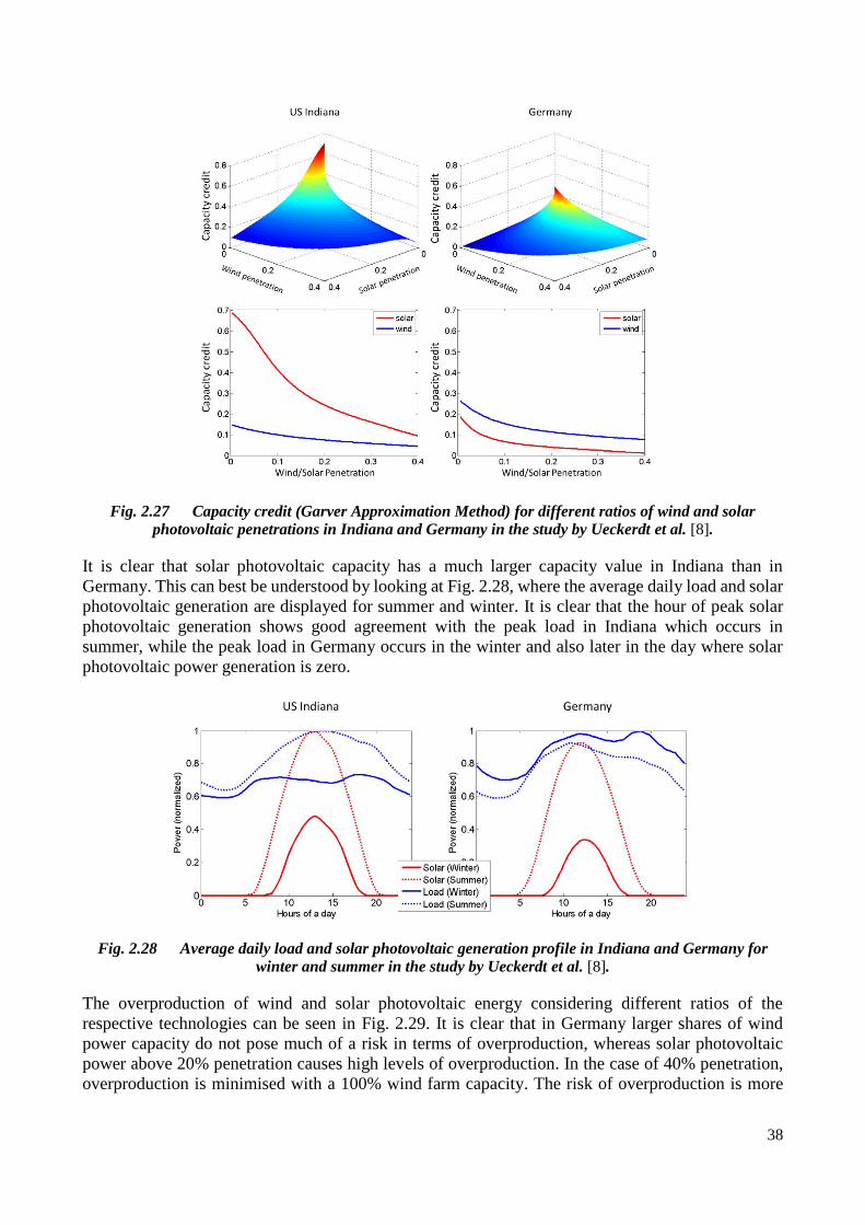
38

Fig. 2.27 Capacity credit (Garver Approximation Method) for different ratios of wind and solar

photovoltaic penetrations in Indiana and Germany in the study by Ueckerdt et al. [8].

It is clear that solar photovoltaic capacity has a much larger capacity value in Indiana than in

Germany. This can best be understood by looking at Fig. 2.28, where the average daily load and solar

photovoltaic generation are displayed for summer and winter. It is clear that the hour of peak solar

photovoltaic generation shows good agreement with the peak load in Indiana which occurs in

summer, while the peak load in Germany occurs in the winter and also later in the day where solar

photovoltaic power generation is zero.

Fig. 2.28 Average daily load and solar photovoltaic generation profile in Indiana and Germany for

winter and summer in the study by Ueckerdt et al. [8].

The overproduction of wind and solar photovoltaic energy considering different ratios of the

respective technologies can be seen in Fig. 2.29. It is clear that in Germany larger shares of wind

power capacity do not pose much of a risk in terms of overproduction, whereas solar photovoltaic

power above 20% penetration causes high levels of overproduction. In the case of 40% penetration,

overproduction is minimised with a 100% wind farm capacity. The risk of overproduction is more

39

balanced in Indiana, where in the case of 40% penetration a ratio of 2:1 would minimise

overproduction (66.6% wind power capacity to 33.3% solar photovoltaic capacity).

Fig. 2.29 Overproduction of renewable energy in Indiana and Germany in the study by Ueckerdt et

al. [8].

Ueckerdt et al. [8] present several conclusions, including the fact that solar penetrations below 20%

are easier to integrate in Indiana than in Germany, but penetrations of above 20% present major

challenges. Wind power integration presented similar challenges in Indiana and Germany.

2.5.3.4 Summary and Critique

Three studies have been presented that study the effect of wind power to solar photovoltaic power

ratios in the United States and Europe. The studies consider different optimisation goals, including

minimising storage capacity, minimising balancing energy, minimising LCOE and maximising

capacity credit.

These studies however did not take into account the effect that variable renewables will have on the

increased costs of conventional generation. Due to the hourly variability of wind and solar

photovoltaic power, the conventional generating fleet is projected to encounter increased ramping

requirements, as well as more stop and start procedures, which will necessarily have a cost

implication. In order to study the effects that different ratios of wind and solar photovoltaic power

could have on a particular conventional generating fleet, detailed grid-level optimal power dispatch

simulations are necessary. Eser et al. [64] performed such a study for five countries in central Europe

for three assumed penetration levels for wind and solar photovoltaic power capacity in 2020, based

on the National Energy Action Plan of Germany.

In the absence of detailed grid-level optimal power dispatch simulations, mean-variance optimisation

(discussed in section 2.6.2 below) could potentially be used to minimise the variance of the residual

load in order to minimise the ramping that would be needed from the conventional generating fleet.

This is explored in the work in this thesis.

2.6 Wind Farm Location Optimisation

2.6.1 Overview

There is a variety of wind farm location optimisation studies available in the literature. Although

some novel approaches have been proposed, the majority of wind farm optimisation studies focus on

40

using mean-variance portfolio theory to optimise the location and size of wind farms. The mean-

variance portfolio theory approach attempts to minimise the variance of combined power output from

wind farms, while some other studies have different optimisation goals, such as minimising the

probability of low power output or minimising losses on the high voltage electricity grid. This section

investigates the wind farm location optimisation studies found in the literature. As this literature

pertains directly to the work undertaken in this thesis, a summary and critique is provided in section

2.6.4.

2.6.2 Wind Farm Location Optimisation using Mean-variance Portfolio Theory

Mean-variance portfolio theory, also known as Markowitz portfolio theory, was first proposed by

Markowitz in 1952 [65]. In mean-variance portfolio theory an investor seeks to minimise risk for a

preferred yield when investing in shares on the stock market. This problem equates well with the

problem of locating wind generation capacity with the view to maximise the cumulative power

contribution whilst minimising variability. Simulated or measured historical wind data sets are used

to simulate theoretical wind turbine power time series using a given wind turbine power curve for

each of the potential locations using one of the methods described in 2.3.2. The covariance between

proposed wind farm locations (equated to risk) is minimised for different capacity factors (equated to

mean portfolio return). The problem translates to a quadratic programming problem that can be solved

for given capacity factors to yield a set of solutions known as the efficient frontier. Solutions on the

efficient frontier represent a mathematically optimal mix of wind farm capacities and locations with

a minimum level of variance for a given mean capacity factor. More details on the mathematical

formulation are provided in section 5.2.

In 2005 Hansen performed a small wind farm optimisation study in North Carolina using mean-

variance portfolio theory [66]. The study was useful for introducing the method but at the time

however, there was no large scale wind data available and the study relied upon measured wind speed

data from three sites which was collected in different years, which somewhat limited the adequacy of

the results. The measured wind speed data was used to simulate wind power time series using the

Vestas 1.6 MW turbine. The study also proposed using mean-variance theory on a subset of the time

series data, in hours that represented peak demand periods in winter and summer.

Mean-variance portfolio theory has been proposed to solve offshore wind farm location optimisation

in the UK by Drake and Hubacek [67] in 2007, but the mathematical details of how the optimisation

is performed were not provided. Wind speed data was obtained from four buoys located at least 40 km

from the nearest coastline and the wind power time series were simulated using the Vestas V90

3.0 MW wind turbine power curve. The authors noted that using buoys located closer to the coastline

(in the order of 1.5 km to 3 km) would have been ideal, as this represented the actual typical location

of offshore wind farms, but this data was not available. The study considered the allocation of 2.7 GW

of wind farm capacity in two scenarios. In the first scenario the 2.7 GW would be located in a single

location and in the second scenario the capacity would be distributed across four locations using

mean-variance portfolio theory. The results indicated that the wind power variability could be reduced

in the order of 36% as a result of the optimal distribution. With many possible solutions of minimised

variance for a given mean power output on the efficient frontier, this study also proposed picking a

solution on the efficient frontier with the maximum power generation per unit of risk. In mean-

variance portfolio theory this is sometimes referred to as the coefficient of variation, and is simply

calculated as the standard deviation divided by the mean.

Hansen and Levine performed a wind farm mean-variance study in 2008 using measured wind speed

data from 95 locations in the United States [68]. The study considered optimal distributions of wind

farm capacity within states, namely Texas, Kansas, Minnesota, and North Dakota as well as an

41

optimal distribution considering all locations within the Midwest Reliability Organization region

(comprising Minnesota and North Dakota). The authors noted that using more than three years of data

would be ideal in order to capture the effect of inter-annual variation, but the available data only

overlapped to cover the whole of 2004. The measured wind speed datasets were scaled to the correct

heights using the wind profile power law and converted to wind power time series using the 2 MW

Vestas V80 wind turbine power curve. The optimisation results confirmed that distributing wind

farms optimally across different sites caused a drastic reduction in the time duration in which there is

zero power production. Traube at al. [69] expanded upon the work of Hansen and Levine by

expanding the geographic area of the study, expanding the timeframe of the study to three years

(2002–2004) at the cost of losing some data sets which did not completely cover this period and

including solar photovoltaic power systems. The wind power time series were simulated as before

while the solar photovoltaic time series were simulated for an idealized 1-axis polar mount tracking

photovoltaic system with a maximum power point (MPP) tracker. The study considered the optimal

allocation of 100 MW of renewable energy capacity, although the authors noted that the choice of

100 MW was essentially arbitrary and the results could easily be scaled up. The results indicated that

expanding the timeframe of the study from one year to three years did not have a significant impact

on the results, while expanding the geographic area significantly decreased the variability of the

combined wind power output. It was also observed that including solar photovoltaic power systems

resulted in a portfolio with 18% lower variability than the optimised wind portfolio alone.

Cassola et al. [70] presented a wind farm mean-variance study of wind farm locations in Corsica, the

fourth largest island in the Mediterranean off the coast of France, using three years (1 October 1996

to 30 September 1999) of measured wind speed data from ten measurement stations on the coastal

regions around the island, averaged over three hours. Even though the physical area of the study is

relatively small, the authors cite their previous research [71] that confirms that Corsica contains at

least two so-called distinct wind climate regimes, i.e. different winds with different intensities,

durations and, most importantly, different areas where they typically occur. The previous research

also separated the wind measuring stations into three distinct anemological regions (clusters) based

on the wind speed time series, the result of which is carried over to the mean-variance study. The

authors also detail how the wind speed measurements, which were measured at a height of 10 m, are

scaled to the correct turbine height. This method is validated using measured wind speeds from an

actual wind farm located close to one of the measurement stations. The wind speed time series is

converted to wind power time series using the Enercon E40/600 wind turbine power curve, which

has a rated power of 600 kW and hub height of 50 m, and again validated by comparing it with power

time series obtained from a similar turbine at the actual wind farm. The optimisation procedure is

performed for the three anemological regions as well for the 10 individual sites, and it is found that

the results are very similar, indicating that using a clustering methodology could be a useful way of

reducing the overall computational time required for the optimisation procedure. In this study, the

results presented did not include the efficient frontier as is customary for mean-variance studies, and

instead the minimum variance, maximum energy and minimum coefficient of variance portfolios are

given special attention. The optimisation procedure was repeated using a different wind turbine power

curve (Enercon E48/800, rated power of 800 kW) and confirmed that the results are turbine

independent, i.e. the optimised portfolio weights stayed largely the same even when a larger wind

turbine power curve was used.

Roques et al. [72] performed a study on the optimal wind power deployment in Europe using the

mean-variance portfolio approach in 2009. The paper also gives a brief review of where mean-

variance portfolio theory had been utilised in other energy planning studies outside of wind farm

location planning. This study used historical hourly wind production data from five countries, namely

Austria, Denmark, France, Germany and Spain for the period from 2006 until 2007. The study

42

considered both unconstrained portfolios and constrained portfolios where national wind resource

potential and transmission constraints were taken into account, with the view to optimising the wind

farm capacity allocation of 2020. As in the study by Hansen [66], this study also investigated the

optimisation of wind farm locations to cover peak demand hours by applying the procedure to a subset

of the time series data, thereby contributing to system reliability. Although the constrained portfolios

reduce the potential for wind power variance minimisation, the authors conclude that there is still a

lot of room for variance reduction, especially compared to the actual projected wind farm allocations

for 2020 in the respective countries. The choice of whether to minimise the overall variance of wind

power or just the variance in peak hours also had a considerable effect on the optimal solutions and

the authors suggest that policy makers should consider which objective is more relevant. The paper

recommends relieving cross-border network constraints and improving the integration of European

electricity markets so as to allow for the maximum reduction of wind power variability through

geographic diversification.

In 2010, Degeilh and Singh [17] presented a precise mathematical formulation of using mean-

variance portfolio theory for wind farm location optimisation, along with a comprehensive small-

scale case study in Texas where several reliability impacts are also investigated. The study considered

the optimal allocation of 40 3 MW wind turbines across seven positively correlated sites and seven

sites with minimal correlation. The study simulated wind power time series using the Vestas V90

3.0 MW wind turbine power curve and three years of wind data from 30 000 sites in the Western

Wind and Solar Integration Study (WWSIS). This was one of the first studies that used mesoscale

wind data comprising many sites over a large area. Reliability impacts, such as the loss of load

probability (LOLP) were investigated using the 1996 IEEE RTS model in combination with Monte

Carlo methods to account for mechanical and electrical failures of wind turbines. This paper also

proposed the idea of incorporating the load data into the mean-variance procedure, effectively

attempting to minimise variance of the residual load, i.e. the load that remains after the combined

wind power output has been subtracted. In the paper however, the authors state that unless the

simulated wind power profiles are shown to have a strong positive correlation with the load, the

optimisation procedure effectively reduces to the mean-variance problem without considering load.

Models based on mean-variance portfolio theory has been developed by Rombauts et al. [73] that

take into account cross-border transmission-capacity constraints in Europe. This work build on the

work done by Roques et al. [72] in two ways. The first is that cross-border capacities are modelled

more explicitly so that the electrical power flows stemming from wind-power production can be

analysed. The second improvement is that different datasets within countries are used instead of

datasets aggregated by country. This study also differed from other studies in that it proposed that the

risk component be defined as the variance of hourly wind power differences, instead of the usual

variance of cumulative wind power output. This is simply achieved by taking the difference

(differential) of the wind power output signal from the time series. The authors present three models

that consider the cases when cross-border transmission-capacity is zero, infinity and a certain limited

value. The case study defined three fictitious countries, namely country A, B and C, that utilised

historical wind data from the Dutch meteorological service, converted to wind power using a Vestas

112 3 MW wind turbine power curve. The case study considers the optimal allocation of 12000 MW,

with the constraint that 5000 MW, 3000 MW and 4000 MW needed to be installed in country A, B

and C respectively. In the third model, where cross-border transmission constraints were considered,

the transmission constraints were defined as 200 MW between A and B, 100 MW between A and C

and 300 MW between B and C (and vice versa). Results indicate that the transmission constraints

increase the minimum standard deviation (variability) in hourly wind power differences by a factor

of √3 . This study revealed some interesting insights into the role of cross-border transmission

constraints on wind farm location optimisation, but the major shortcomings of the study are the

43

fictitious nature of the case study and that the rest of the power system components, as well as

transmission losses are ignored.

In 2015, mean-variance portfolio theory has also been used to simultaneously optimise wind farm

and concentrated solar power station locations in Spain and Portugal by Thomaidis et al. [74]. The

authors present a brief review of both the pieces of literature that are supportive and pessimistic about

the potential of wind power production and the role of spatial diversification. The lack of transmission

infrastructure is highlighted as a major constraint to geographically diverse wind farm portfolios and

references are also included that draw attention to the inter-annual variability of wind power

production. It is stated that wind and solar energy often have complementary profiles and that the

literature is sparse on the potential of this meteorological pattern to reduce the risk of renewable

energy supply. The viability of including concentrated solar power in the mean-variance optimisation

procedure is thus investigated. The study employs the WRF mesocale method to derive three years

(2008–2010) of wind speed and solar irradiance data for 2237 sites in the southern part of the Iberian

Peninsula on a 9 km spatial resolution. Wind power simulations are achieved using the Vestas V90

2 MW wind turbine power curve. The concentrated solar power plants are modelled as parabolic

trough systems according to a model developed by Zhang et al. [75], and more details about the

concentrated solar power simulations are given in a previous paper by some of the same authors [76].

Special attention is given to the procedural implementation of the mean-variance procedure, namely

the Niedermayer and Niedermayer variant of the critical line method, which is particularly efficient

when solving large-scale portfolio selection problems. The authors also mention that the original

spatial resolution of the WRF mesocale model was reduced from 3 km to 9 km, and the energy

generation for the wind and concentrated solar sources were averaged across each day in order the

reduce the computational burden of the optimisation procedure. This study thus considers variance in

daily renewable energy generation and not on an hourly scale like most of the previous studies. The

special procedural implementation of the optimisation procedure and the spatial and temporal

resolution reduction point to the difficulties encountered when the mean-variance problem becomes

sufficiently large. The case study does not specify the size of renewable energy generating capacity

considered, and it is therefore assumed to be an arbitrary capacity that can be scaled up. In the results

section the outcomes of a wind only scenario is compared with a wind and concentrated solar power

combined scenario, with a focus on maximum return, minimum variance and minimum coefficient

of variation portfolios. The efficient frontiers for wind only and combined portfolio scenarios are the

same for high values of capacity factor (30% and above), which simply illustrates that wind farms

exist that have higher capacity factors than concentrated solar power plants and that choosing a high

return value will result in a portfolio made up exclusively of wind farms whether concentrated solar

plants are considered or not. This is not to say that concentrated solar power plants can not contribute

to increased renewable energy supply security, it only highlights the fact that the combined capacity

factor will be lower when concentrated solar power plants are considered. The minimum coefficient

of variation portfolios for the two scenarios best illustrate the effect of considering concentrated solar

power plants in the mean-variance procudure, with the coefficient of variation reducing from 0.52 in

the wind only scenario (16.71 standard deviation as % of capacity, 32.42% capacity factor), to 0.22

in the combined scenario (5.61 standard deviation as % of capacity, 25.49% capacity factor). Out of

the 2237 sites considered, only 34 wind power sites and 42 concentrated solar power sites play any

role in the efficient frontiers (defined as having a non-zero weight in at least one solution on the

efficient frontier), which the authors regard as encouraging when considering the practicality of the

solutions. The authors also note that some low capacity factor wind power sites are included in the

efficient frontier solutions, which might not be financially feasible in any real-world scenario. It is

suggested that a similar study could be conducted on a European scale, but that a dimensionality-

reduction method would be essential. It is suggested that clustering techniques, such as those

44

employed by Zagouras et al. [77], is investigated as a means to make large scale mean-variance

studies realisable.

2.6.3 Other Wind Farm Location Optimisation Methodologies

There are several studies found in literature which also focus the location and size optimisation of

wind farms, but do not use the mean-variance optimisation procedure. These studies either use other

financial portfolio optimisation methods, novel variance minimisation methods or pursue a different

optimisation goal altogether.

Grothe and Schnieders [21] presented a study in 2010 which focused on a copula theory method to

simulate wind speed data and to distribute wind farm capacity optimally. Instead of minimising the

variance of the cumulative wind farm output as in the mean-variance method, the value-at-risk (VAR)

is optimised, i.e. the low power output value which has a certain probability of occurring, also referred

to as tail risks in finance theory, is maximised. The probability, 𝛼, is specified by the user, and the 𝛼-

quantile is maximised so that (1 − 𝛼) ∙ 100% of cumulative power outputs are above the 𝛼-quantile.

A case study for Germany was conducted, considering two scenarios with the 𝛼 values considered

ranging from 0.01 to 0.12. In the first scenario the size and location of the existing capacity is ignored

and it is assumed that the capacity can be relocated, which is not a realistic assumption, but is simply

useful for comparing the performance of the optimal allocation with that of the existing capacity. In

the second scenario the existing capacity is included and optimally expanded by 40%, with the new

capacity being placed in optimal locations. The optimal portfolios were constructed using the wind

time series modelled by the copula functions which had a time resolution of 24 hours. The optimal

portfolios were then evaluated using measured wind speed time series which had daily and hourly

frequencies. The wind speed time series were converted to wind power time series by scaling them

to the correct height and then implementing a piecewise-defined function approach to simulate the

performance of a GE 1.5 MW turbine. The case study also considered whether offshore wind farm

locations can be considered or not and what effect that has on the optimal portfolios. Results indicate

that there is not enough wind farm capacity in the north of Germany, especially considering offshore

sites. Expanding the existing capacity by 40% would entail placing most of the new capacity in this

northern region and could increase the power output available at a certain probability in the order of

100%. Even though the modelled time series had a time resolution of 24 hours, the resulting optimal

portfolios were shown to increase the VAR at an hourly scale as well.

A robust optimisation approach to wind farm diversification was presented by Liu et al. [78] in 2013.

This paper assessed the work and case study done by Degeilh and Singh [17], discussed in section

2.6.2, as well as a case study from the Netherlands. Their criticism of the mean-variance method

included the fact that the procedure is sensitive to the input data, specifically the mean and covariance

matrix. In order to make the wind farm diversification procedure more robust, the authors present a

conditional value-at-risk (CVAR) approach. The conditional value-at-risk, also referred to as the

expected shortfall, is the mean value of a portfolio returns that fall below a probability, 𝛼, on the

probability distribution. Beyond the CVAR optimisation, the authors also introduce the methodology

to produce robust portfolios, where the assumption is that the probability distribution of wind is not

known a priori, but is instead determined from the candidates of a set of distributions using box

uncertainty and ellipsoidal uncertainty measures. The exact probability distribution might not be

known due to the limited availability of data. The mathematical formulation of the complete

optimisation approach is described in detail, after which the case studies are presented. In the case

study from the Netherlands, 10 years (2001-2010) of daily mean wind speed data from 40

meteorological stations were converted to wind power time series using a piecewise-defined function

approach to simulate the performance of a typical wind turbine with a rated power of 1.5 MW. The

results confirm that the robust portfolios slightly outperform the nominal portfolios, especially as the

45

pre-defined uncertainty measure increases. In the Degeilh and Singh [17] case study the robust

portfolio results in a slightly larger variance than the mean-variance portfolio, 395.22 MW and

381.15 MW respectively. As in Degeilh and Singh [17], an IEEE RTS model combined with Monte

Carlo simulation was also employed to test wind power reliability statistics such as loss of load

expectation (LOLE) and expected energy not supplied (EENS). Results indicate that the CVAR

portfolio performs slightly better than the mean-variance portfolio in terms of the reliability statistics.

Reichenberg et al. [23] presented a wind farm location optimisation study in the Nordic countries and

Germany in 2013 which focused exclusively on attaining a portfolio with the minimum coefficient

of variation. Instead of applying the mean-variance approach, the authors presented an iterative

approach to arrive at the optimal portfolio. At each step a simulated wind time series, i.e. a potential

wind farm site, is added to the portfolio if it results in the lowest combined coefficient of variation.

The weakness of this approach is that the decision to add sites to the portfolio is binary and there is

no optimal weight assigned as in the mean-variance approach. The case study used four years (2006-

2009) of wind speed data from 300 sites that was produced using a HIRLAM mesoscale model, with

a spatial resolution of 11 km. The wind turbine power simulation method is not provided, and instead

the reader is referred to a large scale wind power integration report from where the method was

attained. Similar to previous studies, this paper also considered two scenarios where in the first it is

assumed that there is no existing wind farm capacity and in the second that the new wind farm

capacity has to complement the actual existing capacity. In the scenario where no current capacity is

assumed, the optimal coefficient of variation of the wind capacity portfolio was 0.54, which is

significantly less than the 0.91 that was calculated for the existing capacity. The study found that the

variations in wind power output, considering the existing capacity, can be reduced by about 33% by

considering the optimal future allocations.

Schmidt et al. [79] presented a study on the potential of the diversification of wind farms in Austria

in 2012. The Austrian wind atlas does not provide time series wind speed data that is necessary for a

study like this, therefore the study used wind speed Weibull distribution data from the wind atlas in

conjunction with measured wind speed data from meteorological stations to construct wind time

series using the Iman Conover method. A GIS study eliminated sites that are unsuitable for wind farm

siting (due to factors such as land use and a localised cost of energy higher than the current feed in

tariff), resulting in 4226 potential wind turbine sites. Along with the wind atlas data for the eligible

sites, wind speed data for 2008 from 65 reference meteorological stations were used to construct the

wind time series. The wind time series were converted to wind power time series using a generic wind

turbine power curve with a rated power of 2 MW. More details about the GIS study and the wind

power simulation are provided in another paper by the same authors [80]. The case study considered

the optimisation of three models, which attempted to maximise investor profit, minimise hourly

variation and minimise seasonal variation respectively. This was achieved by constructing custom

cost functions, with the minimum annual energy production and variance given as constraints. The

authors indicate that different values of minimal variance were implemented to ascertain feasible

variance values. There is no variable controlling the overall capacity to be assigned, only the annual

energy to be produced. The case study considered the allocation of wind farms to produce at least

5 TWh of energy annually in each of the three models. Results indicate that the minimum hourly

variation model yielded an hourly standard deviation of 320 MW compared to 366.8 MW for the

minimum seasonal variation model and 383.7 MW for the maximum profit model. The spatial

diversity of the minimum hourly variation model was the highest, with 59 installed sites compared to

26 for the minimum seasonal variation model and 11 for the maximum profit model. The minimum

seasonal variation model, which attained a minimum seasonal variability of 7.5 GWh, presented the

most installed capacity with 1820 MW compared to 1795 MW for the minimum hourly variation

model and 1679 MW for the maximum profit model. The authors conclude that there seems to be a

46

trade-off between lower seasonal variability and lower hourly variability. Even though the paper

references other studies that used the mean-variance method, it is not abundantly clear what

advantages the method presented in this paper are over the mean-variance method.

A method to distribute wind farm capacity optimally was presented by Lowery and O'Malley [20] in

2014. Wind data from the MERRA dataset, obtained to facilitate a case study across Ireland, were

interpolated to increase the spatial resolution and scaled to the correct height using the log wind

profile. The constants in the log wind profile were calculated using wind speed data from different

heights. A piecewise-defined function approach was used to simulate a wind power time series, with

the parameters of the piecewise-defined function being derived from measured wind farm data from

62 actual wind farms. For the optimisation procedure, the authors constructed a custom objective

function by concatenating three objectives, namely variance, mean power output and cost and then

assigning a weight to each objective. Different costs were defined for onshore and offshore wind

farms. The authors then minimised the objective function using a constrained optimisation by linear

approximation (COBYLA) method, which is an optimisation method utilised when the derivative of

the objective function is not known. The authors report that for this case study the optimisation

problem took between 3 and 4.5 hours to solve, which can generally be viewed as inferior to the

mean-variance procedure which can be solved in a matter of minutes depending on the size of the

case study. When the cost objective was omitted from the objective function, the wind farm capacity

was almost exclusively distributed offshore. When cost was taken into account, no offshore locations

were included. It is not immediately clear what benefits this method presents over the mean-variance

method, if any. There is also no efficient frontier to examine all available optimal portfolios, instead

just a handful of optimal solutions based on the user-defined weights in the objective function was

used.

Leenman and Phillipson [81] presented a novel method to distribute wind farms in order to reduce

transmission losses on the high voltage power grid considering regional load profiles. This is quite

different from the other wind farm location studies discussed above. In the literature, this kind of

study falls under Transmission and Generation Expansion Planning (TGEP), with this being a special

variant, namely stochastic generation expansion planning. The losses that occur on the high voltage

power grid are proportional to how far the power has to flow from where it is generated. Wind farms

are typically located according to the wind resource and not necessarily close to load centres, and as

such there is the potential for increased transmission losses. The authors present a novel three-step

procedure for optimal wind farm placement. First, the DC power flow model is applied to the network

structure and the load data. Secondly, the potential wind power profiles are simulated using measured

wind speed data. Thirdly, the stochastic optimisation procedure is solved using a simple heuristic

method. The paper presents an overview of power grids and derives a simplified power flow model,

with the simplifications justified in order to facilitate the mathematical programming needed for the

optimisation. The optimisation methodology is explicitly formulated in sufficient detail, after which

the authors also describe how the approach can be adapted so that it can be solved by standard

optimisation software. Network flow duality is utilised to arrive at a nonlinear programming problem,

which is solved by a heuristic method as the investigation of rigorous solution algorithms for

nonlinear programming problems falls outside the scope of this work. A Dutch case study is

presented, where 10 years (2001-2010) of wind data from 50 measurement stations is used. Wind

power time series are simulated using a completely linear piecewise-defined function approach to

approximate a typical 2.5 MW wind turbine. In the case study, the Netherlands is clustered into five

distinct wind zones, with the regional load being aggregated in these distinct wind zones for the DC

power flow model. The optimal locations of wind farms (stochastic generating) is compared with that

of deterministic generating units of varying size and overall capacity. The authors come to several

conclusions, including the confirmation that optimal deterministic unit placement has a much larger

47

effect on reducing transmission losses than stochastic generating units such as wind turbines, which

is to be expected. However, it is noted that there exists a non-trivial relation between the locations of

wind turbines and transportation losses, although this relation only becomes relevant at high

penetration and might be more pronounced in countries with large power networks such as the United

States or Australia. This study also compares its distribution strategy with the mean-variance method

and concludes that at current low levels of wind energy penetration, locating wind farms to minimise

transmissions losses might be advisable, whereas at large levels of penetration (specified as 30% or

more) the spatial diversification achieved by mean-variance optimisation could potentially become

more important.

2.6.4 Summary and Critique

Several wind farm location optimisation studies that are found in the literature have been presented.

The majority of papers use a variant of mean-variance portfolio optimisation for wind farm

diversification, although there are ample examples of studies that have employed other methods.

In terms of the studies that have utilised mean-variance optimisation, the majority of the studies use

measured data pertaining to specific locations instead of mesoscale wind data which covers a large

geographical area. Although measured wind speed is slightly more accurate than mesoscale model

wind data, it is generally accepted that mesoscale wind data fully capture the daily and seasonal cycles

observed in a given location, which is the critical component considered in mean-variance

optimisation. Therefore using measured data from the available weather stations has the potential to

underestimate the full potential of mean-variance approach, as not all potential wind farm locations

in a given area are considered. The time resolutions used in the studies also varied according to the

data that was available, ranging from hourly to daily averages, which makes it difficult to compare

the obtained results as different variations in wind power output are being optimised. Several studies

mention the possibility of including solar power in the mean-variance procedure, but only two papers

follow through on this, one including solar photovoltaic power simulations [69] and the other

concentrated solar power simulations [74]. The sizes of the case studies are also generally quite small,

far below the capacity of wind farms which might be installed on a national scale. There are two

problems with the mean-variance method that arises as the problem size is scaled up, namely the

computational burden of the optimisation procedure and the practicality of the solutions on the

efficient frontier. Neither of these problems are fully addressed in any of the studies, although in the

small case study presented by Cassola et al. [70] a time series clustering approach based on the

measured wind speeds is implemented and mooted as a possible solution to the increasing

computational burden that a larger study might present. Although time series clustering is not

implemented in the study by Thomaidis et al. [74], the authors also propose in their conclusion that

these techniques could aid the mean-variance optimisation procedure. There also is a strong case to

be made for the wind power output to match the given load profile. In pursuit of this goal, two of the

studies [66][72] have implemented the mean-variance approach on a subset of the time series data,

effectively minimising the variance of wind power output during peak hours. Degeilh and Singh [17]

proposed that the load time series could be incorporated into the mean-variance optimisation

procedure, but that unless the wind power profiles exhibited significant correlations with the load, the

exercise would amount to very little gain, and as such this formulation was not implemented in their

study.

In terms of studies that utilised methods other than the mean-variance optimisation, two studies

[7, 36] also implemented optimisation methods from finance theory, namely the VAR and CVAR

optimisation methods. Both of these methods minimise tail risks, which translates to the probability

of low wind power output when considering wind farm diversification. Occurrences of low wind

power output will typically have to be covered by peaking plants which run on more expensive fuels

48

than other plants. The weaknesses of these approaches lie in the fact that the probabilities of high

power output are not considered, which also present financial implications such as increased cycling

of conventional generation or curtailment of wind power output. These portfolio optimisation

approaches also present various challenges as the size of the case study and datasets become

sufficiently large. Three other wind farm location optimisation methods have been presented

[23, 79, 20], although it seems that they pursue the same goals as mean-variance optimisation and it

is not clear what advantages they provide over mean-variance optimisation, if any. They generally

present longer run times and less clarity on the variability reduction potential on offer. One study has

been presented that locate wind farm capacity to minimise transmission losses on the high voltage

power grid [81], but the authors of this study conclude that it is more suited when penetrations of

wind farm capacity are below 30%, i.e. when wind contributes less than 30% of the overall energy in

a given timeframe.

2.7 Time Series Clustering

2.7.1 Overview

Time series clustering has been suggested as a possible addition to the mean-variance optimisation

procedure (applied to renewable energy integration), but only implemented in one small-scale case

study [70] where the time series clustering was done on the wind speeds and not the wind power

output. This section gives an introduction to time series clustering, the different methods and

validation measures, as well as examples in literature where time series clustering has been used in

renewable energy integration studies and mean-variance portfolio studies.

2.7.2 Introduction to Time Series Clustering

Time series clustering is an established field of data mining [82]. It is an unsupervised classification

which attempts to order unlabelled time series into groups of time series data which share common

behaviours or features. The intended outcome of a time series clustering procedure is to end up with

clusters where time series within the same cluster are as similar as possible, while at the same time

being as dissimilar from the time series associated with other clusters. In 2005 Liao [83] published a

review paper on the clustering of time series data, with another review published by Aghabozorgi et

al. [82] in 2015.

Traditionally the main challenges with time series clustering have been the high dimensionality, the

presence of noise and the high feature correlation. There are different approaches to time series

clustering. The approaches to time series clustering have been separated into three groups, namely

raw-data-based, feature-based and model-based clustering by Liao [83] as can be seen in Fig. 2.30.

49

Fig. 2.30 The three different approaches to time series clustering as presented by Laio [83].

In 2001, Halkidi et al. [84] published a paper on cluster validation measures in which they

summarised the steps of the clustering process as can be seen in Fig. 2.31. This summary is also

applicable to time series clustering. First, the selected feature is extracted, which depends on the data

in question and the intended application of the clustering result. Next, several clustering methods are

applied to the data. In determining the appropriate type of clustering algorithm to use, it is generally

suggested to apply several algorithms and then determine the best one for the given case by

considering several standard cluster validation measures. After the appropriate clustering method is

selected (along with an appropriate number of clusters to use), the final clusters are derived and

interpreted.

The focus of this investigation is on the similarity of the hourly power output time series of wind and

solar photovoltaic plants in different geographical locations, therefore the raw-data-based approach

is investigated. If different regions were to be clustered according to diurnal or seasonal features,

feature-based and model-based clustering could be of more use. In raw-data-based time series

clustering, it is necessary to specify a similarity measure, which is explained further below.

50

Fig. 2.31 The steps of the clustering process in the study by Halkidi et al. [84].

2.7.3 Similarity Measures

The similarity measure, also sometimes referred to as the distance measure or dissimilarity measure,

determines how the similarity between two time series is measured, and is chosen based on the

characteristics of the input data and the intended application of the cluster results. The similarity

measure determines whether similarity in time, similarity in shape or similarity in change will be

targeted. Typical similarity measures used in time series clustering include Lp-norm distance (also

known as the Mikowski distance), Dynamic Time Warping distance (DTW), Longest Common

Subsequence (LCSS) distance and the Pearson's correlation factor.

2.7.4 Clustering Methods

Different clustering methods exist to cluster time series data. Several complex clustering algorithms

have been proposed, but the basic clustering algorithms can be classified as either hierarchical or

partitional.

2.7.4.1 Hierarchical Methods

Hierarchical clustering is a clustering method in which a series of partitions takes place that result in

nested clusters organised as a hierarchical tree that can easily be visualized using a dendrogram. It is

not necessary for the user to specify the number of clusters a-priori.

2.7.4.2 Partitional Methods

Partitional clustering divides the datasets into a user-specified number of subsets. There are many

different types of partitional clustering methods, of which the k-means algorithm is the most widely

used.

2.7.4.3 Other Methods

51

Many other types of clustering algorithms that have been suggested for time series data include fuzzy

c-means clustering, density-based clustering and self-organising maps. Clustering methods are an

active research field and several different approaches have been suggested in recent years [82].

2.7.5 Cluster Validation Measures

Cluster validation measures are used to determine the quality of a clustering result. Many cluster

validation measures have been proposed and reviewed in the literature by Arbelaitz et al. [85]. There

is no single clustering method which performs optimally for all types of data. The main purpose of

the cluster validation measures is to aid the user in selecting the appropriate clustering method that

best fits the specific dataset, as well as to provide insight into how many clusters might be appropriate.

2.7.6 Time Series Clustering in Renewable Energy Research

Time series clustering has been used in many renewable energy studies, some of which will briefly

be described here. Burlando et al. [71] used time series clustering techniques to identify anemological

regions and wind regimes on the isle of Corsica in France. Wind speed data from ten weather stations

were used in the study. Three distance measures were combined with five hierarchical clustering

methods to form a total of 15 clustering technique combinations. The results of this study was used

by Cassola et al. [70] to perform a small mean-variance wind farm optimisation procedure. The

weather stations and one of the dendrograms from a hierarchical clustering procedure can be seen in

Fig. 2.32.

Fig. 2.32 The weather stations on the isle of Corsica (left) and an example of a clustering result (right)

from the study by Burlando et al. [71].

Vallée et al. [86] used a feature-based time series clustering technique to cluster 94 wind regions in

Europe with similar statistical behaviour in order to perform adequacy evaluation studies for wind

farms. The authors employed a fast incremental algorithm to cluster the features extracted from the

time series, which was compared with the classic k-means clustering method. The Pearson coefficient

was specified as the similarity measure. The results of the fast incremental clustering can be seen in

Fig. 2.33.

52

Fig. 2.33 The results of the fast incremental clustering of wind parks in Europe by Vallée et al. [86].

Zagouras et al. [77] used clustering techniques to determine coherent zones of Global Horizontal

Irradiance (GHI) for a utility scale territory in California for solar photovoltaic capacity planning

purposes. The k-means clustering method was used to cluster the gridded irradiance data that was

obtained from satellite observations, in conjunction with a principal component analysis based

dimensionality reduction method. Two cluster validation measures were used to verify the quality of

the clustering result, as well as to ascertain the appropriate number of clusters to use. Some of the

coherent solar microclimate zones are shown in Fig. 2.34.

Fig. 2.34 Coherent solar microclimate zones obtained through time series clustering in the study by

Zagouras et al. [77].

2.7.7 Time Series Clustering combined with Mean-Variance Portfolio Theory

Time series clustering has been employed in conjunction with stock portfolio optimisation in the

literature.

53

Tola et al. [87] used the k-means clustering method to cluster historical time series of stocks in order

to improve reliability of share portfolios in terms of the ratio between predicted and realized risk. The

authors used the historical daily returns of 1071 selected stocks on the New York Stock Exchange

during the period 1988–1998 in the study. The time series were partitioned into two subsets. The first

subset was used to cluster the time series, with the clustered daily return time series being used as an

input to the mean-variance portfolio optimisation procedure, and compared to an unclustered mean-

variance result as well as an approach involving random matrix theory filtering. These initial results

represented the predicted risk, with the unclustered solution displaying the lowest predicted risk. The

mean-variance optimisation results were then applied to the second subset in order to determine the

realised risk. The clustered solutions displayed the lowest realised risk, as can be seen in Fig. 2.35.

Fig. 2.35 Predicted risk (solid lines) and realised risk (dotted lines) for the unclustered mean-variance

results (black), the random matrix theory results (red) and the clustered mean-variance result (blue) in the

study by Tola et al. [87].

Nanda et al. [88] employed several clustering methods to cluster stocks on the Bombay Stock

Exchange (BSE). The authors used k-means clustering, self-organising maps and fuzzy c-means

clustering methods to cluster the historical return time series. After consulting several clustering

validation measures, it was concluded that the k-means clustering method resulted in the best

clustering result. Time series from different clusters were selected to be used in a mean-variance

optimisation, with the results being that the inputs from the clusters performing better when compared

to the BSE index.

54

3 Renewable Energy Simulation

3.1 Overview

This section provides the mathematical formulation of the wind power and solar photovoltaic power

simulations that were performed in this study. The wind power simulations are performed using a

multi-turbine power curve approach developed by Norgaard and Holtinen [22], while the solar

photovoltaic power simulations are performed using a simplified approach that is adapted from the

textbook by Masters [14] and the PV Watts simulator that was developed by the National Renewable

Energy Laboratory (NREL) [28].

3.2 Wind Power Simulation

3.2.1 Multi-turbine Power Curve

The multi-turbine power curve approach by Norgaard and Holtinen [22] was used to simulate the

wind power time series from the wind speed time series and a wind turbine power curve. This method

was developed to more accurately simulate the wind power from multiple wind turbines located in a

relatively large area, for which only a single wind speed time series is available. The method is

detailed below in four steps as follows:

Step 1 The first step is to perform a block averaging procedure on the wind speed time series.

The number of points to include in the block average procedure, 𝐵, is given by [22]:

w

D

Bt

(3.1)

where 𝐷 is the spatial resolution of the wind speed time series data, 𝜇𝑤 is the mean wind

speed and ∆𝑡 is the time resolution of the time series data.

The block averaged wind speed 𝑎𝑗 at every point in time 𝑗 is then given by [22]:

2

2

1

1

Bj

j iB

i j

a wB

(3.2)

where 𝑤𝑖 is the wind speed at the ith point in time in the original wind speed time series.

The block averaging procedure is implemented to account for the spatial "memory effect"

of the winds propagating over the specific area with a wind speed similar to the average

wind speed of the site [22].

Step 2 A discrete multi-turbine power curve is constructed from a discrete single turbine power

curve and a normalised Gaussian distribution. The jth discrete point in the multi-turbine

power curve 𝑃𝑚𝑗 is given by [22]:

j j i ii

Pm Ps G (3.3)

where 𝑃𝑠𝑗 is the jth discrete point in the single-turbine power curve and 𝐺𝑖 is the iit discrete

point on the Gaussian distribution. In this investigation the type of single-turbine power

55

curve to be used depends on the average wind speed of the site and is described in

section 3.2.2. The single turbine power curve is effectively convoluted with the Gaussian

distribution as shown in Fig. 3.1. The Gaussian distribution has a standard deviation, σ,

that depends on the assumed wind intensity, 𝐼, and the spatial resolution of the wind speed

time series, 𝐷, as shown in Fig. 3.2. In this investigation a wind speed intensity of 10%

was assumed for all sites. The actual standard deviation of the Gaussian distribution is

obtained by multiplying the normalised standard deviation by the mean wind speed of the

site, 𝜇𝑤 . The offset of the Gaussian distribution is initially zero and is adjusted as

described in the next step. The Gaussian distribution represents the probability

distribution function of the wind speeds present at individual wind turbines at different

locations in the given area.

Fig. 3.1 Gaussian distribution.

Fig. 3.2 The normalised standard deviation of the Gaussian distribution used to construct the multi-

turbine power curve as a function of the spatial resolution of the wind speed time series and the wind

speed intensity [22].

Step 3 As described in step 2, the offset of the Gaussian distribution is initially set to zero. In

order to find the correct offset, the single-turbine power curve is applied to the complete

wind speed time series in order to calculate a total energy yield. The multi-turbine power

curve constructed with the Gaussian distribution with zero offset is also applied to the

complete time series and will necessarily overestimate the energy yield. Norgaard and

Holtinen recommend that the offset be adjusted until the energy yield from the multi-

turbine power curve equals the energy yield from the single-turbine power curve. In this

investigation the offset was adjusted further until the energy yield from the multi-turbine

56

power curve equalled 90% of the energy yield from the single-turbine power curve. This

is justified by the results from a study performed by Harman [89], which found that real-

world power generation results are slightly overestimated when using the single-turbine

power curves as given by the manufacturers due to different environmental and wind

conditions.

Step 4 Once the correct offset has been determined in step 3, the multi-turbine power curve is

applied to the block-averaged wind speed time series to generate the simulated wind

power time series.

3.2.2 Turbine Selection

It is unrealistic to use the same turbine model for every site, as different turbine models are

specifically designed to perform optimally in different wind speed ranges. As such, three different

wind turbine models with the same nameplate capacity (2 MW) from the same manufacturer (Vestas)

had been selected to model the wind power in this investigation. The criterium for the type of wind

turbine to use is simply the average wind speed of the site, 𝜇𝑤, as shown in Table 3.1, and has been

selected based on information provided by the manufacturer [90].

Table 3.1 Wind turbine models with respective average wind speeds. Site Average Wind Speed Wind Turbine Model

𝜇𝑤 ≤ 6.5m/s Vestas V110-2.0 MW IEC IIIA

6.5m/s < 𝜇𝑤 ≤8.5m/s Vestas V100-2.0 MW IEC IIB

𝜇𝑤 > 8.5m/s Vestas V90-2.0 MW IEC IIA/IEC IIIA

An example of the multi-turbine power curve method applied to the Vestas V100-2 MW wind turbine

is shown in Fig. 3.3.

Fig. 3.3 Example of the multi-turbine power curve as applied to a single wind turbine power curve.

3.3 Solar Photovoltaic Power Simulation

The solar photovoltaic power simulations are done at every time step using ambient temperature data

and irradiance data using a methodology that is adapted from the textbook by Masters [14] and the

57

PV Watts simulator [28] by NREL. The solar irradiance is taken as the total irradiance inclined on

cell and consists of the direct irradiance, diffuse irradiance and reflected irradiance components.

First, the cell temperature, 𝑇𝐶𝑒𝑙𝑙, is calculated using the ambient temperature and solar irradiance as

follows [14]:

20

0.8Cell Amb

NOCTT T I

(3.4)

where 𝑇𝐴𝑚𝑏 denotes the ambient temperature, 𝐼 denotes the solar irradiance inclined on the

photovoltaic panel [kW/m2], 𝑁𝑂𝐶𝑇 is the nominal operating cell temperature and is selected as 45 °C

in this investigation. The 𝑁𝑂𝐶𝑇 , which is usually provided by the solar photovoltaic panel

manufacturer, is the expected cell temperature in a module when the ambient temperature is 20 °C

and the solar irradiation is 0.8 kW/m2 [14].

The derating effect of temperature, 𝜂𝑇𝑒𝑚𝑝, is given by [28]:

1 ( )Cell Ref

TempRef

T T

I

(3.5)

where 𝛾 is the temperature coefficient, 𝑇𝑅𝑒𝑓 is the reference temperature and 𝐼𝑅𝑒𝑓 is the reference

irradiance. In this investigation, a temperature coefficient of -0.47%/°C is selected, which is typical

of a standard solar panel module [28]. The reference temperature and reference irradiance is selected

as 25 °C and 1 kW/m2 respectively.

The DC power, 𝑃𝐷𝐶, is calculated as follows [28]:

DC Rated TempP I P (3.6)

where 𝑃𝑅𝑎𝑡𝑒𝑑 is the nameplate direct current power rating of the photovoltaic panel, selected as 2 MW

in order to be of the same magnitude as the wind turbine time series simulation models in section 3.2.

The DC power that the solar photovoltaic panel generates is then converted to AC power using an

inverter, with the inverter efficiency, 𝜂𝐼𝑛𝑣𝑒𝑟𝑡𝑒𝑟, calculated as follows [28]:

0.0059

0.0162 0.0142nomInverter

ref

(3.7)

where 𝜂𝑛𝑜𝑚 is the nominal efficiency of the inverter, 𝜂𝑟𝑒𝑓 is the reference inverter efficiency and 𝜁

is the load fraction, calculated simply as the DC power at that time step divided by the rated power,

𝑃𝐷𝐶/𝑃𝑅𝑎𝑡𝑒𝑑. The nominal efficiency and the reference inverter efficiency are given as 0.96 and 0.9637

respectively. The reference inverter efficiency was calculated by examining actual inverter

performance data from the California Energy Commission [28].

A graph of the inverter efficiency, as it depends on the load factor, is given in Fig. 3.4. It is clear that

the inverter typically reaches the nominal efficiency at load factors of approximately 0.3 and higher.

58

Fig. 3.4 Graph of inverter efficiency versus load factor obtained from equation (3.4).

Finally the AC power, 𝑃𝐴𝐶 , is calculated as

:0

:

0 : 0

DC Inverter DC Rated

AC Rated nom DC Rated

DC

P P P

P P P P

P

(3.8)

In standard cases, the AC power is equal to the DC power multiplied by the inverter efficiency. When

the calculated DC power is greater than the rated DC power, the AC power is simply calculated as

the rated DC power times the nominal efficiency of the inverter.

For the sake of simplicity, many other sources of losses have not been taken into account, including

but not limited to effects from soiling, shading, wiring and ageing.

0

0,2

0,4

0,6

0,8

1

0 0,1 0,2 0,3 0,4 0,5 0,6 0,7 0,8 0,9 1

η I

nv

erte

r

Load fraction ζ

59

4 Time Series Clustering

4.1 Overview

Time series clustering has been suggested in the literature as a method of improving the mean-

variance optimisation procedure. The justification for using time series clustering is given in

section 5.6, which stems from the mean-variance optimisation formulation.

Time series clustering is an established field of data mining. It is an unsupervised classification which

attempts to order unlabelled time series into groups of time series data which share common

behaviours or features. Traditionally the main challenges with time series clustering have been the

high dimensionality, the presence of noise and the high feature correlation [83]. There are also

different approaches to time series clustering which have been separated into three groups, namely

raw-data-based, feature-based and model-based clustering. As the focus of this investigation is on the

correlation of the hourly power output profiles of different geographical locations, the raw-data-based

approach is applied.

This section will give an overview of the complete time series clustering methodology used in this

investigation. The elements in time series clustering include the similarity measure, distance matrix,

clustering method and cluster validation measures.

4.2 Similarity Measure

The similarity measure determines how similar two time series are to each other. The type of

similarity measure that is used determines whether similarity in time, similarity in shape or similarity

in change will be targeted.

The Euclidian distance similarity measure is used in this investigation to quantify the similarity

between two time series. Suppose vectors 𝐗 and 𝐘 are 𝐿-dimensional and represent two time series:

T

1 2 3

T

1 2 3

...

...

L

L

X X X X

Y Y Y Y

X

Y (4.1)

Then the Euclidian distance, D𝐸(𝐗, 𝐘) between the two vectors is formulised as follows [83]:

2

1

, ( )L

E i ii

D X Y

X Y (4.2)

The Euclidian distance is a specific version of the Lq-norm distance, also known as the Minkowski

distance, D𝐿𝑞(𝐗, 𝐘), which is given by [83]:

1

1

, ( )q

L qqL i i

i

D X Y

X Y (4.3)

where 𝑞 is usually selected as 1 (Manhattan distance) or 2 (Euclidian distance). This similarity

measure examines values observed at corresponding points in time, effectively treating observations

in a single time series at different points in time as if they were independent [91]. This is a desirable

characteristic in this application, as it is the intention so cluster simulated power output time series

by comparing their values at a given time independent from values right before or after, in order to

construct a centroid that best represents the power output time series of that cluster. For example, if

60

two potential wind farm sites are clustered together, one with strong power output values during 15:00

to 17:00 and one with strong power output values between 17:00 and 19:00, the one potential site

would be contributing during peak load times while the other would not, and the resulting centroid

would lose a lot of that information. There are similarity measures that could account for time

stretching and time shifting formations such as this, if this fits with the intended application.

4.3 Distance Matrix

The distance matrix is a symmetrical matrix that captures the distance between every vector and stores

it in the off-diagonal elements. The diagonal contains all zeros as the distance between a vector and

itself is zero. The distance matrix stores the similarity between every time series that is included in

the investigation and serves as an input to the clustering method.

Suppose another 𝐿-dimensional vector 𝐙, in conjunction with the previous vectors 𝐗 and 𝐘:

T

1 2 3 ... LZ Z Z ZZ (4.4)

then using the Euclidian distance measure will result in a distance matrix between the three vectors

that looks as follows:

, 0 , ,

Distance Matrix , , 0 ,

, , , 0

E E E

E E E

E E E

D D D

D D D

D D D

X X X Y X Z

Y X Y Y Y Z

Z X Z Y Z Z

(4.5)

The distance matrix serves as an input to the clustering methods. After the distance matrix has been

computed, the different time series can effectively be viewed as data points, with distances between

them specified by the distance matrix. As such, in the following section reference will be made to

data points, with the ith coordinate of the data point being analogues to the ith value in the time series.

4.4 Clustering Methods

The clustering method determines how the cluster operation will be performed. In determining the

type of clustering method to use, it is generally suggested to apply several algorithms and then

determine the best option for the given case, using cluster validation methods. Several clustering

methods have been considered in this investigation. Basic clustering algorithms can be classified as

either hierarchical or partitional.

4.4.1 Hierarchical Methods

Hierarchical clustering makes use of clustering steps that result in nested clusters organised as a

hierarchical tree that can easily be visualised using a dendrogram, as can be seen in Fig. 4.1. It is

therefore not necessary for the user to specify the number of clusters beforehand.

61

Fig. 4.1 Example of a dendrogram.

In hierarchical clustering, the clustering steps can be done in two directions:

Agglomerative: All the data points start as their own cluster, and clusters are then grouped at each

step according to the distances between the clusters. This is referred to as the “bottom up”

approach.

Divisive: All the data points start as one cluster, and clusters are then split at each step according

to the distances between the clusters. This is referred to as the “top down” approach.

The distances between different clusters depend on the type of hierarchical clustering method, as can

be seen in an example in Fig. 4.2 (where only two dimensions are plotted and each data point

represents a time series) with the distance between points being the similarity measure (the Euclidian

distance in this investigation). The cluster centroids represent the average coordinates of all the data

points assigned to the respective cluster. If an agglomerative hierarchical clustering is used, the next

step would be to combine two of the three clusters. If the average distance between points was

considered (centroid distance), cluster 2 and cluster 3 would be combined, but if the maximum

distance was considered, cluster 1 and cluster 2 would be combined as the maximum distance between

a point in cluster 2 and cluster 3 is greater than the maximum distance between point in cluster 1 and

cluster 2.

Fig. 4.2 Example of hierarchical clustering.

The agglomerative hierarchical clustering algorithms considered in this investigation include

complete-linkage, average-linkage and Ward’s method hierarchical clustering.

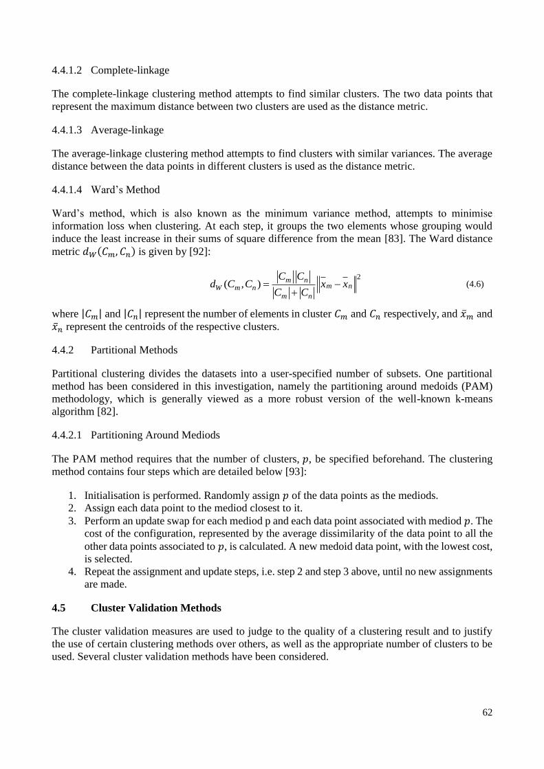
62

4.4.1.2 Complete-linkage

The complete-linkage clustering method attempts to find similar clusters. The two data points that

represent the maximum distance between two clusters are used as the distance metric.

4.4.1.3 Average-linkage

The average-linkage clustering method attempts to find clusters with similar variances. The average

distance between the data points in different clusters is used as the distance metric.

4.4.1.4 Ward’s Method

Ward’s method, which is also known as the minimum variance method, attempts to minimise

information loss when clustering. At each step, it groups the two elements whose grouping would

induce the least increase in their sums of square difference from the mean [83]. The Ward distance

metric 𝑑𝑊(𝐶𝑚, 𝐶𝑛) is given by [92]:

2

( , )m n

m nW m nm n

C Cd C C x x

C C

(4.6)

where |𝐶𝑚| and |𝐶𝑛| represent the number of elements in cluster 𝐶𝑚 and 𝐶𝑛 respectively, and �̅�𝑚 and

�̅�𝑛 represent the centroids of the respective clusters.

4.4.2 Partitional Methods

Partitional clustering divides the datasets into a user-specified number of subsets. One partitional

method has been considered in this investigation, namely the partitioning around medoids (PAM)

methodology, which is generally viewed as a more robust version of the well-known k-means

algorithm [82].

4.4.2.1 Partitioning Around Mediods

The PAM method requires that the number of clusters, 𝑝, be specified beforehand. The clustering

method contains four steps which are detailed below [93]:

1. Initialisation is performed. Randomly assign 𝑝 of the data points as the mediods.

2. Assign each data point to the mediod closest to it.

3. Perform an update swap for each mediod p and each data point associated with mediod 𝑝. The

cost of the configuration, represented by the average dissimilarity of the data point to all the

other data points associated to 𝑝, is calculated. A new medoid data point, with the lowest cost,

is selected.

4. Repeat the assignment and update steps, i.e. step 2 and step 3 above, until no new assignments

are made.

4.5 Cluster Validation Methods

The cluster validation measures are used to judge to the quality of a clustering result and to justify

the use of certain clustering methods over others, as well as the appropriate number of clusters to be

used. Several cluster validation methods have been considered.

63

Four cluster validation metrics have been applied in validating the performance of the clustering

algorithms in this investigation. These include the average between cluster distance, the average

within cluster distance, the average silhouette widths and the Caliński-Harabasz index.

4.5.1 Average Between Cluster Distance

The average between cluster distance represents the average sum of the square distance between data

points clustered together in different clusters. A higher average between cluster distance is desirable

as this indicates better separation between clusters.

4.5.2 Average Within Cluster Distance

The average within cluster distance represents the average sum of the square distance between time

series clustered together in a single cluster. A lower average within cluster distance is desirable as

this indicates less separation between data points in a single cluster.

4.5.3 Average Silhouette Width

The silhouette width of a data point is a measure of the membership strength of that data point to its

assigned cluster. It is based on the average distance 𝑎𝑥𝑡 between each data point 𝑥𝑡 of a cluster 𝐶𝑚 to

every other data point in that cluster, and 𝑏𝑥𝑡, the minimum value of the average distance between

that data point and the data point belonging to all other clusters. The average silhouette width is

defined as [85]:

1

1average silhouette width

max( , )

t t

t k t t

Kx x

k x C x x

b a

T b a

(4.7)

where 𝑇 denotes the number of data points and 𝐾 denotes the number of clusters. Note that the

difference between 𝑏𝑥𝑡 and 𝑎𝑥𝑡

is normalized by their maximum value. The average silhouette width

metric results in a score between -1 and 1, where -1 one indicates a very poor clustering and 1

represents a very good clustering.

4.5.4 Caliński-Harabasz Method

The Caliński-Harabasz (CH) index calculates the ratio between cohesion and separation, where

cohesion is based on the distances from the points in a cluster to its centroid and the separation is

based on the distance from the centroids to the global centroid, i.e. the centroid of all the data

points [94]. It is defined by the relationship:

( ) / ( 1)

Caliński-Harabasz index( ) / ( )

B

W

Tr S K

Tr S T K

(4.8)

with

2

1

( )K

kB kk

Tr S T x x

(4.9)

and

64

2

1

( )

t k

K

kw tk x C

Tr S x x

(4.10)

where 𝑇 denotes the number of data points, 𝐾 denotes the number of clusters, 𝑆𝐵 and 𝑆𝑊 denote the

traces of the between-class and the within-class scatter matrices respectively, 𝑇𝑘 denotes the number

of number of data points in cluster 𝑘, 𝑥𝑡 denotes a data point in cluster 𝑘, �̅�𝑘 denotes the centroid of

cluster 𝑘 and �̅� denotes the centroid of all the data points. The CH index is normalised to account for

the increasing number of clusters. The objective of the CH method is to determine a number of

clusters 𝐾 that maximises the CH index. This implies maximising the ratio of 𝑇𝑟(𝑆𝐵) and 𝑇𝑟(𝑆𝑊),

i.e. the ratio of between cluster scatter and within cluster scatter.

4.6 Determining the Number of Appropriate Clusters

There is no definitive way to determine the number of clusters that is appropriate for a given dataset.

It is suggested that the results of the cluster validation measures are consulted. The number of clusters

is typically chosen to represent a point where increasing the number of clusters yields diminishing

returns in the cluster validation measures, as formalised in the L-method [95].

4.6.1 Wind Time Series

The wind power time series show significant variance between different time series, and as such it

has been decided that the average centroid error will be consulted in order to determine the optimal

number of clusters. The number of clusters is chosen so the centroids display an average centroid

error of less than 10%. The average centroid error is formulised as follows:

A centroid data time series, �̅�𝑘, is calculated for each cluster and the total error at each point in time

𝑖 between the centroid time series and every time series 𝑥𝑡 in the cluster 𝐶𝑘 is summed and averaged

to calculate the average centroid error. The average centroid error is defined by the relationship:

1 1

1average centroid error

t k

K L

ki tik x C i

x xL T

(4.11)

where 𝐿 denotes the number of length of the time series, 𝑇 denotes the number of time series, 𝐾

denotes the number of clusters and �̅�𝑘𝑖 and 𝑥𝑡𝑖 represents the ith record of centroid �̅�𝑘 and time series

𝑥𝑡 respectively.

4.6.2 Solar Photovoltaic Time Series

The solar photovoltaic power time series show more correlation than wind power time series, and as

such it is decided that all the cluster validation measures will be inspected using the L-method, in

order to ascertain how many clusters might be appropriate.

The L-Method [95] attempts to find the 𝐾 best number of clusters by fitting 2 linear models to the

left hand side and right hand side of a cluster validation method dataset and determining a point 𝑐

such that the total root mean square of the linear models is minimized. The cluster validation method’s

values, each corresponding to a number of clusters, is split into two groups such that the left hand

group 𝐿𝐶 has values {2,…, c} and right hand group 𝑅𝐶 has values {c,…, b}, where b represents the

maximum number of clusters. After a linear model is fitted to each group using linear regression, the

total root-mean-square error (RMSET) is given by the relationship:

65

1

RMSE RMSE RMSE1 1

T L R

c b c

b b

(4.12)

The RMSE of the left and right hand groups, RMSEL and RMSER respectively, are weighted

proportional to the lengths of 𝐿𝐶 and 𝑅𝐶 . The crucial point is found by finding the value 𝑐 that

minimizes RMSET.

66

5 Mean-Variance Optimisation

5.1 Overview

In mean-variance portfolio theory, an investor seeks to minimise risk for a preferred yield when

investing shares on the stock market [96]. This problem equates well with the problem of locating

wind generation capacity with the view to maximise the cumulative power contribution whilst

minimising variability and has been applied extensively in the literature in this regard.

This section will give an introduction and mathematical formulation to mean-variance portfolio

theory. This section will also introduce the addition of solar photovoltaic power time series and load

time series into the optimisation problem. Studies in the literature have suggested that solar

photovoltaic power and load data be incorporated, but no study has actually implemented this. Some

studies has also suggested that clustering techniques be incorporated into the optimisation procedure.

The incorporation will be justified at the end of this section.

5.2 Introduction to Mean-variance Portfolio Theory

Mean-variance portfolio theory, which was first proposed by Markowitz in 1952 [65], provides a

mathematical framework to select a portfolio of assets, each with an associated historical return time

series, that minimises the risk of the combined portfolio. The investor provides a desired mean return

on his portfolio, which acts as a constraint in the optimisation problem, and the optimisation is solved

such that an optimal weight of each asset is found that results in a cumulative return with minimum

variance. The portfolio return column vector, 𝐑, is defined as:

1 1 2 2 3 3 ... ...t t T Tw w w w w R H H H H H (5.1)

where 𝐇𝑡 denotes the historical return of asset 𝑡, 𝑤𝑡 denotes the weight of asset 𝑡 and 𝑇 is the total

number of assets. Each historical return vector looks as follows:

T

1 2 3 ... ...t i LH H H H HH (5.2)

where 𝐻𝑖 is the return at time 𝑖 and 𝐿 is the length of the historical return vector (time series).

The optimisation problem is formulised as follows [96]:

1 2 3( , , ,..., ) 1 1

min var( ) j l jl

t T

T T

w w w w w j l

w w

R (5.3)

such that

Desired1

,t

T

tt

w

(5.4)

Total1

t

T

t

w w

(5.5)

and

min max , 1...Tt t tw t (5.6)

67

where 𝑤𝑡 is the decision variable that results in a minimised cost function, var(𝐑), which is the

variance of cumulative portfolio return vector 𝐑. Variable 𝑇 is the total number of assets, 𝜎𝑗𝑙 denotes

the covariance between the return time series 𝐇𝑗 and 𝐇𝑙 of asset 𝑗 and 𝑙, 𝜇𝑡 is the mean value of return

time series 𝐇𝑡 of asset 𝑡, 𝜇Desired is the desired mean return of the cumulative portfolio, 𝑤Total is the

total weight that can be assigned and min𝑡 and max𝑡 are the minimum and maximum weight

respectively that can be assigned to asset 𝑡.

The total weight, 𝑤Total, is normally specified as 1, which results in the weights assigned to assets,

𝑤𝑡, falling between 0 and 1 subject to their respective minimum and maximum weights, min𝑡 and

max𝑡.

Equation (5.3) can alternatively be written as follows:

T

1 2 3

T

...

min var( )

Tw w w w

w

R w w (5.7)

where 𝐰 is a 𝑇 × 1 vector that represents the weights of each asset, Σ is the covariance matrix and

𝐰𝐓 indicates the transpose of vector 𝐰 (which is not to be confused with 𝑤𝑡, which indicates the Tth

element of column vector 𝐰). The covariance matrix, Σ, is positive semi-definite, which means that

𝐰𝐓Σ𝐰 is non-negative for every non-zero column vector 𝐰 of 𝑇 real numbers.

Covariance is a measure of how two random variables, 𝑋 and 𝑌, vary together, and is calculated as

follows [97]:

1

1cov( , ) ( )( )

L

XY i ii

X Y X X Y YL

(5.8)

where 𝐿 is the length of the random variables and �̅� and �̅� represent the mean values of 𝑋 and 𝑌

respectively.

The covariance calculation can also be written as:

cov( , ) E[( E[ ])( E[ ])]X Y X X Y Y (5.9)

where E[ ] represents the expected (mean) value function.

The covariance matrix, Σ, which is also known as the dispersion matrix or variance–covariance matrix

[96], contains the variance of each random variable in its diagonal and the covariance between the

random variables in the off-diagonal elements:

var( ) cov( , )

cov( , ) var( )

X X Y

Y X Y

(5.10)

with cov(𝑌, 𝑋) = cov(𝑋, 𝑌).

The mean-variance portfolio theory formulation translates to a quadratic programming problem.

Quadratic programming problems are formulated as follows [98]:

An 𝑛-dimensional vector, 𝐱, is found that will

68

T T1

minimise2

x Qx c x (5.11)

subject to 𝑚 constraints in the form

Ax b (5.12)

where 𝐜 is a real-valued n-dimensional vector, 𝐐 is a symmetric real-valued 𝑛 × 𝑛 -dimensional

matrix, 𝐴 is a real 𝑚 × 𝑛-dimensional matrix and 𝐛 is an 𝑚-dimensional real vector. The notation

𝐀𝐱 ≤ 𝐛 means that every entry of the vector 𝐀𝐱 is less than or equal to the corresponding entry of the

vector 𝐛.

When observing equation (5.7) and the linear constraints in equation (5.4)-(5.6), it is clear that the

mean-variance optimisation problem takes the form of a quadratic programming problem with the

vector 𝐜 specified as a zero column vector.

The mean-variance problem can be solved for different given desired mean returns, 𝜇Desired, to yield

a set of solutions known as the efficient frontier. Every point on the efficient frontier represents a

portfolio with a minimum variance for the given desired mean return as can be seen in Fig. 5.1. The

extreme points on the efficient frontier to the far left and far right represent portfolios that are made

up exclusively of one asset with the lowest and highest returns respectively (in the absence of

constraints that limit the weight of individual assets).

Fig. 5.1 The efficient frontier in the mean-variance portfolio optimisation problem.

5.3 Mean-variance Portfolio Theory Mathematical Formulation with Wind Power

Mean-variance portfolio theory will be formalised here as applied to wind farm location optimisation.

Potential wind farm sites, 𝑥 , are viewed as assets (𝑡 in section 5.2) and simulated or measured

historical wind data sets are used to simulate theoretical wind turbine power time series using a given

wind turbine power curve for each of the potential locations. The simulated wind power time series,

𝐏𝑥, is equated to historical return time series (𝐇𝑡 in section 5.2). The covariance between proposed

wind farm locations (equated to risk) is minimised for different capacity factors (equated to mean

portfolio return).

The mathematical formulation of the optimisation problem is similar to section 5.2:

69

1 2 3( , , ,..., ) 1 1

min var( ) j l jl

x N

N N

w w w w w j l

w w

W (5.13)

such that

Desired Wind1

,x x

N

x

w

(5.14)

Total Wind1

x

N

x

w w

(5.15)

and

0 max , 1...Nx xw x (5.16)

where 𝑤𝑥 is the number of turbines at site 𝑥, var(𝐖) is the variance of the cumulative wind power

output vector 𝐖, 𝑁 is the total number of potential wind farm sites, 𝜎𝑗𝑙 is the covariance between the

wind power time series 𝐏𝑗 and 𝐏𝑙 of site 𝑗 and 𝑙, 𝜇𝑥 is the mean wind power output 𝐏𝑥 of site 𝑥,

𝜇Desired Wind is the desired mean wind power output of the cumulative wind power output 𝐖 from

all sites, 𝑤Total Wind is the total number of wind turbines that can be assigned and max𝑥 is the

maximum number of turbines that can be assigned to site 𝑥.

In equation (5.16), instead of a 0, a min𝑥 term (minimum number of turbines) can be included for

two reasons:

If there is a minimum number of turbines that is specified to be built on a certain site (this might

lead to a sub-optimal solution).

If the mean-variance optimisation is performed with existing wind farm capacity in mind, the

historical or simulated wind power time series of the existing wind farm capacity would be

included and the existing capacity would be specified as the min𝑥 term.

The capacity factor of the cumulative wind power output is simply the mean cumulative wind power

output divided by the total capacity as follows:

Desired Wind

Total Wind

capacity factorw

(5.17)

Therefore solving for different values of 𝜇Desired Wind yields the efficient frontier. Solutions on the

efficient frontier representing a mathematically optimal mix of wind farm capacities and locations

with a minimum level of variance for a given overall capacity factor.

When performing the mean-variance optimisation with wind farms, the wind turbine power curves

that are used to simulate the wind power time series should satisfy one of two criteria:

The wind turbine power curves should have the same rated power.

If the wind turbine power curves don’t have the same rated power, the wind turbine power curves

should all be normalised to a selected rated power, with the total assigned capacity decision

variable (𝑤𝑥, number of turbines) resulting from the optimisation procedure being scaled using the

same respective normalising factor.

70

This is to ensure that the trivial solution is avoided where wind power capacity is assigned to the site

where a wind turbine with a higher rated capacity is used.

5.4 Mean-variance Formulation with Wind Power and Solar Photovoltaic Power

When incorporating solar photovoltaic power into the mean-variance optimisation problem, it is

possible to treat the potential solar photovoltaic sites just as potential wind farm sites and perform the

optimisation just as in section 5.3, with the variance of the total renewable power output being

minimised. However, this would cause some confusion with the mean power output variable,

𝜇Desired, as wind farms and solar photovoltaic farms typically have very different capacity factors.

wind farms typically display capacity factors larger than 25%, whereas solar photovoltaic farms

typically display capacity factors of 18% to 25%. The 𝜇Desired variable would now represent the

mean renewable power output. Solving the mean-variance optimisation problem in the usual way

would lead to solutions on the lower end of the efficient frontier being dominated by solar

photovoltaic farm capacity and solutions to the higher end being dominated wind farm capacity. This

is obviously not desirable, as the objective should be to have a high capacity factor wind farm

portfolio that is supported by solar photovoltaic power. This can be solved by setting up the linear

constraints in a slightly different way. The approach that is defined here considers the total wind farm

capacity that is to be assigned and the desired overall wind farm capacity factor, and simply allows

the optimisation procedure to supplement the wind power output with solar photovoltaic power output

in order to minimise the variance of the total renewable power output, with several optional

constraints related to the solar photovoltaic power capacity.

First, the total renewable power output is defined as:

1 1

N Mx y

i i ix y

R W S

(5.18)

where 𝑅𝑖 is the total renewable power output at time 𝑖, 𝑁 is the number of wind farms, 𝑊𝑖𝑥 is the

wind power output at wind farm 𝑥 at time 𝑖, 𝑀 is the number of solar photovoltaic farms, 𝑆𝑖𝑦

is the

solar photovoltaic power output at solar photovoltaic farm 𝑦.

Combining the total renewable power output at all times 𝑖, results in the total renewable power output

vector 𝐑 of length 𝐿:

T

1 2 3 ... LR R R RR (5.19)

The mean-variance problem is then formulised as follows:

1 2 3( , , ,..., ) 1 1

min var( ) j l jl

x N M

N M N M

w w w w w j l

w w

R (5.20)

such that

Desired WindWind

,x x

N

x

w

(5.21)

Min Desired SolarSolar

,x x

M

x

w

(5.22)

71

Total WindWind

,x

N

x

w w

(5.23)

Max Total SolarSolar

x

M

x

w w

(5.24)

and

0 max , 1...N+Mx xw x (5.25)

where 𝑤𝑥 is the number of turbines or solar photovoltaic capacity at site 𝑥, var(𝐑) is the variance of

cumulative renewable power output, 𝑁 is the total number of potential wind farm sites, 𝑀 is the total

number of potential solar photovoltaic farm sites, 𝜎𝑗𝑙 is the covariance between the power time series

of site 𝑗 and 𝑙, 𝜇𝑥 is the mean power output of site 𝑥. The sites included in the optimisation procedure

are classified as either potential wind farm sites (𝑥 ∈ Wind) or potential solar photovoltaic farm sites

(𝑥 ∈ Solar). The desired mean wind farm output, 𝜇Desired Wind, and the total wind farm capacity

(number of wind turbines) to be allocated, 𝑤Total Wind, is specified by the user. Equation (5.22) and

(5.24) are optional constraints that control the minimum overall solar photovoltaic farm power output,

𝜇Min Desired Solar , and the maximum solar photovoltaic farm capacity that can be allocated,

𝑤Max Total Solar. As before, max𝑥 is the maximum number of turbines or solar photovoltaic farm

capacity that can be assigned to any one individual site 𝑥.

Similar to the wind turbine power curve scaling procedure in section 5.3, the simulated solar

photovoltaic power time series would typically be scaled to the selected rated power of the wind

turbine power curve in order to have decision variables (𝑤1, 𝑤2, 𝑤3, … , 𝑤𝑁+𝑀) that refer to the same

capacity, although this is not necessary with the formulation of the constraints given above due to the

separation of wind capacity and solar photovoltaic capacity constraints. For example, if a simulated

power time series of a 2 kW solar photovoltaic panel is included in conjunction with simulated power

time series of 2 MW wind turbines, the simulated power time series of the 2 kW solar photovoltaic

panel would be scaled to 2 MW so that the decision variables could be compared as is.

5.5 Mean-variance Formulation with Wind Power, Solar Photovoltaic Power and Load

In section 5.3 and 5.4 the variance or the total wind power output and the variance of the total

renewable power output was minimised respectively. As renewable power plants have no fuel costs

and don’t emit any greenhouse gases, they are usually given priority dispatch over conventional

generation plants and are only curtailed in extreme events. This effectively means that the

conventional generation fleet has to meet the residual load, i.e. the load minus the contribution of

renewables. It is therefore intuitive to want to minimise the variance of the residual load in order to

maximise the use of cheaper and more efficient base-load and load-following plants over peaking

power plants.

Incorporating the load time series into the mean-variance formulation was suggested (but not

implemented) by Degeilh and Singh [17]. The authors considered only wind farm capacity and load,

and proposed that unless the wind farm time series showed considerable correlation with the load, the

incorporating the load time series has a very small effect. In the case of wind power only, where the

cumulative wind power output, 𝐖, is the weighted total of the power time series of the individual

sites 𝐏𝑥:

1 1 2 2 3 3 ... ...x x N Nw w w w w W P P P P P (5.26)

72

and the weight vector 𝐰 is consists of the respective weights:

1 2 3 ... Nw w w ww (5.27)

the variance of the cumulative wind power output is:

T

1 1 2 1

2 1 2 2T

1 2

2

1

var( )

var( ) cov( , ) cov( , )

cov( , ) var( ) cov( , )

cov( , ) cov( ) var( )

var( ) 2 cov( , )

N

N

N N N

N

x x x y x yx x y

w w w

W w w

P P P P P

P P P P Pw w

P P P P P

P P P

(5.28)

Degeilh and Singh [17] showed that when the load is included in the variance formulation, the

variance of the residual load reduces to:

2

1 1

var( ) var( ) var( ) 2cov( , )

var( ) var( ) 2 cov( , ) 2 cov( , )N N

x x x y x y x xx x y x

w w w w

L W L W L W

L P P P L P (5.29)

The formulation of the variance of the residual load thus contains four terms. The first term, var(𝐋),

is fixed. The second term, the variances of the power outputs of individual sites var(𝐏𝒙), is controlled

by a squared variable 𝑤𝑥2. The third term, the covariances between power outputs of individual sites

cov(𝐏𝒙, 𝐏𝒚), is controlled by a cross product variable 𝑤𝑥𝑤𝑦. The last term, the covariances between

the load and the power output of individual sites, cov(𝐋, 𝐏𝒙), are controlled by a single degree variable

𝑤𝑥. Due to the nature of these controlling variables, Degeilh and Singh [17] proposed that the last

term, which captures the interaction between the load and the power output of individual sites,

contributes much less to variance than the second and third terms, and that unless the power output

of individual sites showed considerable correlation with the load, the mean-variance optimisation

would essentially reduce to the case where the load was not included.

However, it is hypothesised that when both the wind power time series and solar photovoltaic power

time series are used in conjunction with the load time series, the combined power profiles of wind

farms and solar photovoltaic farms might show good correlation with the load, and an optimal ratio

of wind farm capacity to solar photovoltaic farm capacity could be obtained. This technique takes

into account the shape of the daily load profile and could result in a more country specific distribution

of renewable power capacity. The mathematical formulation will now follow.

The residual load is given by

R Ti i iL L R (5.30)

where 𝐿𝑖𝑅 is the residual load at time 𝑖, 𝐿𝑖

𝑇 is the total load and 𝑅𝑖 is the total renewable power output.

Combining the residual load at all times 𝑖, results in the residual load vector 𝐋𝑹 of length 𝐿:

T

1 2 3 ...R R R R RLL L L L

L (5.31)

73

The mean-variance problem is then formulised as follows:

1 2 3 1

1 1

( , , ,..., ) 1 1

min var( ) j l jlx

N M

N M N MR

w w w w w j l

w w

L (5.32)

such that

1 1,w (5.33)

Desired WindWind

,x x

N

x

w

(5.34)

Min Desired SolarSolar

,x x

M

x

w

(5.35)

Total WindWind

,x

N

x

w w

(5.36)

Max Total SolarSolar

x

M

x

w w

(5.37)

and

0 max , 2...1 N+Mx xw x (5.38)

This formulation is similar to the formulation in section 5.4, except that the load time series is

included as the first time series in conjunction with the negative of the wind power time series and

solar photovoltaic power time series, meaning that 𝑤1 is the decision variable that refers to the load

time series. As can be seen in equation (5.33), this decision variable is set to one. This leaves the

optimisation procedure with decision variables 𝑤2,…,𝑤1+𝑁+𝑀 to assign to the negative wind power

time series and negative solar photovoltaic power time series in order to minimise the variance of the

residual load.

5.5.1 Load Time Series Pre-processing (Detrending)

Any multi-year load time series that is obtained from actual data is likely to display annual growth or

decline trends in the load. It is therefore necessary to remove the annual trend from the load before

including the load time series in the mean-variance optimisation procedure, resulting in a load time

series where every year of load data has the same mean value. Failing to remove the annual trend

would in all likelihood invalidate the results of the optimisation procedure as sites with coincidental

low power output in lower load years might be preferred to the actual optimal solution, with the same

occurrence possible for higher load years and sites with coincidentally higher power output during

those years.

In this investigation, it has been decided to remove the seasonal trend from the load data as well when

it is used in the mean-variance optimisation procedure. The goal of the mean-variance optimisation

procedure is ultimately to minimise the variance of the residual load around the mean, and therefore

a constant mean load is required throughout the year. It is hypothesised that leaving the seasonal trend

in the load data would only be useful if renewable power sources with extremely seasonal variability

are included in the optimisation problem, which is not the case here. It is therefore left as a future

research question. It is important to keep in mind that the standard deviation of the residual load

74

obtained in this investigation refers to the standard deviation of the residual load with its seasonal

trend removed, whereas the load data with its seasonal trend still intact (which represents the real

world scenario) is used to calculate all the key performance indicators.

5.6 Time Series Clustering Justification

The quadratic programming problem allows for a ceiling constraint for each site, max𝑥, but not a

floor constraint. This implies that, while upper limits can be imposed on the capacity assigned to

individual locations, the lower limit equates to zero (when there is no minimum capacity that is

assigned or there is no existing capacity on that site). It is therefore impossible to assign a minimum

capacity that would justify the fixed cost infrastructure needed to support a wind farm or solar

photovoltaic farm on that site. This is problematic because the solutions on the efficient frontier often

assign low capacities to certain sites, which makes part of the solution unfeasible in the face of

practical and economic considerations. The capacities are furthermore assigned to exact coordinates,

depending on the spatial resolution of the input data, yielding a very rigid solution when factors such

as land use, grid connection capacity, etc. have not been taken into account. There is no clear site

selection alternatives should a specific site be disqualified based on these considerations and the

optimisation has to be performed again with the adjusted constraints.

The optimisation strategy can be combined with time series clustering, thereby optimising the

distribution of wind power capacity in terms of geographical areas with similar wind power profiles

rather than individual potential wind farm sites. In order to define geographical areas with similar

wind power profiles and solar photovoltaic power profiles, potential wind farm sites and solar

photovoltaic sites are clustered according to the temporal similarity of the associated simulated power

time series. An averaged power profile, referred to as a centroid, is derived for each cluster by

averaging the power at each time instant for all locations assigned to that cluster. The total wind

power capacity, supplemented by solar photovoltaic power capacity, is then optimally distributed

amongst the clusters with the mean-variance portfolio methodology, using the centroids as an input.

75

6 Key Performance Indicators related to Renewable Power Integration

6.1 Overview

In order to compare the results of the optimisation procedure, it is necessary to select several key

performance indicators. This section provides the mathematical formulations and the reasoning

behind the selection of the key performance indicators.

Before the key performance indicators are formulised, several variables are introduced that will be

used throughout this section. The total renewable power, 𝑅𝑖, which is the total wind power output and

solar photovoltaic power output at a given time, is given by:

1 1

N Mx y

i i ix y

R W S

(6.1)

where 𝑁 is the number of wind farms, 𝑊𝑖𝑥 is the wind power output at wind farm 𝑥 at time 𝑖, 𝑀 is

the number of solar photovoltaic farms, 𝑆𝑖𝑦

is the solar photovoltaic power output at solar

photovoltaic farm 𝑦.

The residual load, which is the load minus the renewable power output, is given by

R Ti i iL L R (6.2)

where 𝐿𝑖𝑅 is the residual load at time 𝑖 and 𝐿𝑖

𝑇 is the total load at time 𝑖.

6.2 Standard Deviation of Renewable Power Output/Residual Load

The goal of the mean-variance optimisation is to minimise the variance of the combined input time

series. In the case where only the wind power is included in the mean-variance formulation, the

variance of the cumulative wind power output is minimised. In the case where solar photovoltaic

power is included, the variance of the cumulative renewable power output is minimised. If load is

also included in the procedure, the variance of the residual load time series is minimised.

In each of the formulations of the mean-variance procedure, the standard deviation, 𝑠, of any time

series 𝑥, is calculated as follows [97]:

2

1

1( )

1

L

ii

s x xL

(6.3)

where 𝐿 is the length of time series 𝑥 and �̅� is the mean of time series 𝑥.

6.3 Mean Absolute Load Ramp Rate

The mean absolute load ramp rate provides a measure of the intra-hour differences in load. It is

expected that larger penetrations of renewables will increase the variability of the residual load and

thereby also increase the intra-hour differences in load that will cause conventional generators to

cycle more and increase the need for peaking power plants. The mean absolute load ramp rate is

defined as follows:

Mean Absolute Ramp Rated

E Ldt

(6.4)

76

where 𝐿 is either the load time series or the residual load time series, 𝑑

𝑑𝑡 is the differential and 𝐸[ ] is

the expected value (mean).

6.4 Capacity Credit

In order to approximate the capacity credit, the Garver approximation-based method is used, as

discussed in section 2.5.2.3. Instead of considering the full load and residual load datasets, the Garver

capacity value formulation considers two different subsets of the residual load data, 𝐻1 and 𝐻2, which

represents the highest 𝛼% of loads and residual loads respectively. This is similar to the approach

employed by Madaeni et al. [56], and is reported to provide a better approximation of the true capacity

credit because the peak load periods are isolated. The Garver 𝛼% highest load capacity value is given

by [56]:

1

2

Garver % Highest Load Capacity Value ln

Ti

Ri

L

i H

L

i H

e

mm

e

m

(6.5)

where 𝑚 is the system characteristic, 𝐿𝑇 and 𝐿𝑅 are the load time series and the residual load time

series respectively, 𝑖 represents the ith data point in the time series with 𝐿 data points. Because

detailed generating unit data of the Eskom fleet is unavailable, the system characteristic 𝑚 is assumed

to be 4% of peak load as is consistent with the literature [8]. In this investigation 𝛼 is selected as 5%,

which is a compromise between the lower percentage that would be considered in the case of solar

photovoltaic power only and the higher percentage that would be considered in the case of wind

power only.

The capacity credit is calculated from the capacity value and the nameplate capacity of the installed

renewable power plants as follows:

capacity value

capacity creditnameplate capacity

(6.6)

The capacity credit can be calculated for the wind farm capacity or solar photovoltaic farm capacity

separately, or a combined capacity credit can be calculated.

6.5 Generator Capacity by Type

The goal of the generator capacity by type metric is to use a high-level statistical approach to estimate

the size and type of generators that will be needed to supply the load/residual load. This approach

was described in the study by Tarroja et al. [60], and is discussed in more detail in section 2.5.2.4.

The approach is formulised as follows:

Each of three type of generators, namely base-load, load-following and peaker plants are assigned a

duration period length, which represents the typical average time that the specific type of generator

will be online. The duration period lengths are given in Table 6.1.

77

Table 6.1 Generator Type Duration Period Lengths [60]. Generator Type Duration Period Length Typical generator types

Peaker ≤5 h Natural-gas brayton cycle

Reciprocating engines

Load-following 6-168 h Natural-gas combined cycle

Natural-gas rankine cycle

Natural-gas brayton cycle

Base-load 169+ h Nuclear rankine cycle

Coal-powered rankine cycle

Gasified coal-powered combined cycle

Next, the base-load, load-following and peaker plant totals are initialised to 0 MW. Generator

duration lengths are obtained by examining the residual load time series at different power levels

which are increased by equal increments, Pinc, from zero. Pinc is specified as 10 MW in this study

similar to the study by Tarroja et al. At each power level, the periods of generator operation at or

above that power level are located and each of their duration recorded. A graphical representation of

this process is presented in Fig. 6.1. The generator duration lengths (t1, t2, t3, …) are grouped

according to duration period lengths of the different type of generators. Pinc is then divided into three

parts in the same proportion as the generator duration length groupings and added to the base-load,

load-following and peaker plant totals.

Fig. 6.1 Visualisation of the generator duration counts metric (adapted from Tarroja et al. [60]).

A similar example to the one that was provided in the literature review in section 2.5.2.4, will now

be provided here to clarify the procedure. If at 28 GW, zero of the generator duration lengths are

longer than 168 hours, two thirds of the generator duration lengths are between 6 hours and 168 hours

and the remaining third of the generator duration lengths are less than 6 hours, 0 MW will be added

to the base-load total, 6.66 MW will be added to the load-following total and 3.33 MW will be added

to the peaker total. In effect this means that the marginal demand at between 28 GW and 28.01 GW

will be served by load-following plants 66.6% of the time and by peaker plants 33.3% of the time.

After this process is repeated for successive power levels up until the maximum value of the net load

signal, the totals for the different types of generators are obtained.

78

The generator capacity by type metric is applied to the load before subtracting any renewable power,

and then applied to the residual load obtained from optimised renewable distributions to ascertain the

different types of capacity that will be needed in the future to meet the load with different penetrations

of renewable power plants.

79

7 Data Acquisition and Processing

7.1 Overview

The data that was required to perform the renewable energy simulations and optimisation procedures

were obtained from different sources. This section details the sources and acquisition of all the

relevant data.

7.2 Grid GIS Data

In order to collect the data that is necessary for renewable energy simulation, it is necessary to know

the location of high voltage power lines in South Africa. It is unlikely that renewable power plants

will be built far away from the grid, and as such the physical location of the grid will dictate where

data for renewable energy simulation should be collected.

Geographic information system (GIS) files of the South African high voltage grid (88 kV up to

765 kV) was obtained from Eskom and can be seen in Fig. 7.1. The GIS files include existing lines,

as well as planned lines that will be built in the next 15 years from the time of this study.

Fig. 7.1 Existing and planned high voltage power lines in South Africa.

7.3 Wind Data

Wind speed data was obtained from the WASA project (described in section 2.4.2.2). The WASA

project includes hourly wind speed and wind direction time series data from 1 Jan 1990 until 31 Dec

2012. The dataset includes 527 time series, each falling on a 27 km x 31 km grid, for a large area

covering parts of the Northern Cape, Western Cape and Eastern Cape. Only sites within 50 km from

the existing and planned high voltage network were included in the study, as can be seen in Fig. 7.2.

Any datasets that were offshore were also excluded. This resulted in 402 sites that would be included

in the study.

80

Fig. 7.2 Complete WASA dataset and sites included in the study.

7.4 Solar Photovoltaic Data

7.4.1 Solar Irradiance Data

Solar irradiance data was obtained from the SoDa service (described in section 2.4.3). The SoDa

service allows the user to select the coordinates of the data that the user requires. A 40 km x 40 km

grid was drawn across South Africa and solar irradiance data was collected for all grid points that fall

within 50 km from the existing and planned high voltage network, which resulted in 590 solar

irradiance time series datasets, as can be seen in Fig. 7.3.

Fig. 7.3 SoDa dataset that was collected for this study.

81

The type of solar radiation data that was collected was the inclined irradiance, which consists of three

components, namely the direct irradiance, diffuse irradiance and the reflected irradiance. The three

components combined give the total inclined irradiance, also referred to as the global inclined

irradiance. Each dataset was downloaded with the optimum angle corresponding with the optimal

solar photovoltaic angle map provided by the Department of Environmental Affairs [99] as shown in

Fig. 7.4. The optimal solar photovoltaic angle represents the tilt angle of the solar photovoltaic panel

that would result in the maximum annual energy generation. It was assumed that the solar

photovoltaic panels face north. The irradiance data that was downloaded represented hourly data from

1 February 2004 until 31 December 2012.

Fig. 7.4 Optimal solar photovoltaic angle map from the Department of Environmental Affairs [99].

7.4.2 Temperature Data

Temperature data was obtained from the South African Weather Service (SAWS). It was not possible

to obtain temperature data from all the weather stations. A total of 38 weather stations were selected

that fell along the high voltage electricity grid, as can be seen in Fig. 7.5. The requested temperature

data spanned from 1 January 2005 until 31 December 2012. Unlike the wind speed data and solar

irradiance data however, many of the temperature time series contained significant quantities of

missing data.

82

Fig. 7.5 Selected weather stations (from SAWS) for temperature data acquisition.

In order to replace the missing data in the temperature records, a linear regression technique was used.

A linear model was constructed for each temperature time series that was trained with the known

values and the corresponding temperature records from the nearest four temperature stations. This

linear model was then used to fill in the missing values.

7.5 National Load Data

Hourly national load data was obtained from Eskom for the period from 1 January 2000 until 31

March 2015. The peak load in South Africa typically occurs in winter, and the winter and summer

load profiles have markedly different shapes as can be seen in Fig. 7.6.

83

Fig. 7.6 Typical week of summer and winter load.

The load data contained significant annual growth and decline trends. In order to use the load time

series in the mean-variance optimisation procedure, it was necessary to remove the annual and

seasonal trends as discussed in section 5.5.1. In order to calculate the key performance indicators,

only the annual trend is removed, which maintains the higher mean values that is observed during

winter months.

Removing the annual trend effectively caused the entire load time series to resemble the peak load

year, which in this case was 2007, along with the random fluctuations that occurred in each year.

Throughout the case studies in the results section, reference is made to the current load. This is a

reference to the key performance indicators as applied to the detrended load data without any

renewable power subtraction.

7.6 Overlap of Data

The period that wind data, solar radiation data, temperature data and load data overlapped was from

1 Jan 2005 until 31 Dec 2012. This represented eight years of hourly data and was deemed sufficient

to account for the inter-annual variability of wind power and the relationship between weather

phenomena and load. The leap days in 2008 and 2012 were removed, leaving 70 080 hourly records

(8 years x 365 days x 24 hours). All the case studies were performed using this subset of time series

data.

84

8 Software Implementation

8.1 Overview

The complete methodology was implemented using two software packages, namely Matlab and

R Studio. Matlab was used for the initial data cleaning and renewable energy simulation, due to its

speed. The time series clustering, mean-variance optimisation, key performance indicator

calculations and GIS file outputs were performed in R Studio due to the availability of a range of

packages that facilitated the above-mentioned procedures. An overview of the software

implementation can be seen in Fig. 8.1.

Fig. 8.1 Overview of the software implementation.

This section gives an overview of the software programs and the software implementation, including

the workflow and the respective Matlab and R packages that were used.

8.2 Renewable Power Time Series Simulation in Matlab

Matlab is a numerical computing environment that contains a proprietary object-oriented

programming language. Matlab is used in academia and industry across a wide range of topics

including science, engineering and economics [100]. Matlab was chosen for the data cleaning and

renewable power simulation due the speed of Matlab code computation, which stems from the

efficient use of vector and matrix calculus inherent in the programming language. Matlab code can

either be entered into the command window, or saved as a script in the Matlab editor. In the following

part of this section, each flowchart represents a separate Matlab script.

Data Aquisition

• Described in Section 7

Renewable Power

Simulation

• Performed in Matlab

Time series Clustering

• Performed in R Studio

Mean-variance

Optimisation


Key Performance

Indicator Calculation


Output of Results


85

8.2.1 Wind Power Simulation

The wind power time series are simulated using the wind speed data and the methodology described

in section 3.2. The flowchart for this process can be seen in Fig. 8.2. The input and output data are

stored as CSV files (Comma Separated Values).

Fig. 8.2 Flowchart of the wind power simulation procedure in Matlab.

The curve-fitting toolbox in Matlab is used to convert discrete data points for the single wind turbine

power curve and the multi-turbine power curve into a function that can be applied to any analogue

wind speed.

8.2.2 Solar Photovoltaic Simulation

The first step in the solar photovoltaic power simulation is to condition the temperature data using

the method described in section 7.4.2. By conditioning it is meant that missing data is calculated using

a linear regression method by considering the four closest stations whose data is not missing. The

flowchart for this process can be seen in Fig. 8.3. The input and output data are stored as CSV files.

Fig. 8.3 Flowchart of the temperature data cleaning procedure in Matlab.

The next step is to simulate the solar photovoltaic power time series using the conditioned temperature

data and the solar radiation data with the method described in section 3.3. The flowchart for this

process can be seen in Fig. 8.4. The input and output data are stored as CSV files.

Matlab

Data cleaning using linear

regression method

(described in section 7.4.2)

Raw Temperature

.csv files

Cleaned Temperature

.csv files

Wind speed

.csv files

Matlab

Wind power simulation

(described in section 3.2)

Wind power time

series .csv files

Wind turbine

power curves

.csv files

86

Fig. 8.4 Flowchart of the solar photovoltaic power simulation procedure in Matlab.

8.3 Time Series Clustering, Mean-variance Optimisation and Key Performance Indicator

Calculation in R Studio

R Studio is an open-source integrated development environment for the R programming language.

The R programming language is an implementation of the S programming language and is most often

used for data mining, optimisation and statistical analysis [101]. R implementations are highly

extensible through various packages to which a very active R community contribute. R was chosen

for the time series clustering, mean-variance optimisation and the key performance indicator

calculations for two reasons:

The availability of R packages that can facilitate time series clustering procedures, optimisation

procedures and GIS file plotting and editing.

The ability of R to perform high-quality data visualisation.

Similar to Matlab, R code can either be entered into the command window, or saved as a script using

the R studio editor. The time series clustering, mean-variance optimisation and key performance

indicator calculations were all implemented in a single R script. The flowchart for the R script can be

seen in Fig. 8.5. The inputs are the renewable energy simulations that were performed in section 8.2

and are in comma-separated-value (CSV) format. The output of the R script is graphs of the key

performance indicators and GIS files that represent the clustered areas with their associated optimal

renewable energy capacity.

Solar Photovoltaic

Power Time series

.csv files

Solar Radiation

.csv files

Matlab

Solar photovoltaic power

simulation (described in

section 3.3).

Cleaned

Temperature

.csv files

87

8.3.1 Flowchart of the Complete R Studio Script

Fig. 8.5 Flowchart of the time series clustering, mean-variance optimisation and key performance

indicator calculation in R Studio.

8.3.2 R Packages Used

Table 8.1 contains each external R package that was used in the study, as well as the purpose for

which it was used. Table 8.1 does not list packages that are included in the base R distribution.

R Studio

Time series clustering is

performed and the

appropriate method and

number of clusters is

selected for wind power

and solar photovoltaic

power. Centroid time series

are generated (described in

Chapter 4).

R Studio

Mean-variance optimisation

is performed (described in

Chapter 5).

R Studio

The load data is detrended

(described in section 5.5.1).

R Studio

Key performance indicators

are calculated, graphed and

analysed (described in

Chapter 6). Optimal

solutions are selected.

Wind power time

series .csv files

Solar Photovoltaic

Power Time series

.csv files

Load time series

.xlsm file

Clustered regions

with associated

optimal renewable

power capacities

.gis files

Graphs of results

.jpg files

88

Table 8.1 Summary of R packages used in this study (excluding base R packages). Package Name Description Purpose in this study

ggplot2 A package that implements a novel

plotting system in R that is based on the

grammar of graphics methodology by

Leland Wilkinson.

Used to plot various results.

quadprog A package that contains a quadratic

programming algorithm.

Used to perform the mean-variance optimisation

(quadratic programming).

cluster A package that contains several well-

known clustering algorithms

Used to perform the PAM clustering method.

fpc Flexible Procedures for Clustering. A

package that contains various methods

for clustering and cluster validation.

Used to perform the average silhouette width and

Caliński-Harabasz index cluster validation

measures.

sp A package providing classes and

methods for spatial data.

Used to import, manipulate and export spatial

data.

rgeos Interface to The Geometry Engine Open

Source (GEOS), a free program library

in C ++ for handling two- and 2.5-

dimensional geometries

Used to manipulate spatial data.

alphahull A package that contains functions to

compute the alpha-shape and alpha-

convex hull of a given sample of points

in a plane.

Used to create alpha hull shapes (GIS files) for

clustered regions.

89

9 Case Studies and Results

9.1 Overview

The chapter provides the results obtained using the complete methodology on a South African case

study. The wind speed data, solar irradiance data and temperature data time series has been used to

simulate wind power time series and solar photovoltaic time series. The simulated power time series

has been clustered using time series clustering techniques. The clustered wind and solar photovoltaic

time series have been used in conjunction with load data in mean-variance optimisation procedures

to optimise the distribution of renewable power capacity in four different case studies that use the key

performance indicators to assess the results. Hourly data from 1 January 2005 until 31 December

2012 (excluding leap year days) is used.

This chapter is divided into four parts:

Section 9.2: The results of the renewable power simulation procedures is presented.

Section 9.3–9.4: The results of the time series clustering applied to the simulated wind power time

series and solar photovoltaic time series.

Section 9.5–9.8: The results of four case studies which investigated the use of clustered wind and

solar photovoltaic time series in conjunction with mean-variance optimisation. Table 9.1 provides

a summary of the four case studies that have been performed.

Section 9.9: Several investigations have been performed that pertains to the work which is not

included in this thesis. A brief overview of the results is given in this section.

Table 9.1 Summary of Case Studies Case

Study

Description Summary

1 Different Formulations

of Mean-variance

Optimisation

In the literature mean-variance portfolio theory has been applied to minimise the

variance of wind power. This case study examines the effect of including the solar

photovoltaic power time series and the load time series in the optimisation

procedure.

2 REIPPPP Round 1-3

vs. Optimisation

(Unclustered and

Clustered)

This case study compares the optimisation procedure (considering wind power,

solar photovoltaic power and load) with the wind farm and solar photovoltaic farm

allocation in the REIPPPP, in order to quantify the benefits of the optimisation

procedure when compared with a real world allocation in South Africa. This case

study also justifies the use of time series clustering by examining the effect that

time series clustering has on the results of the optimisation procedure when

compared to the unclustered optimisation as found in the literature.

3 Optimal Future

Penetrations of Wind

and Solar Photovoltaic

Power in South Africa

This case study uses the optimisation procedure to allocate a range of future

penetrations of wind power capacities with complementing solar photovoltaic

power capacities in South Africa, in order to study the effect that increasing

penetrations of renewable energy will have on the conventional generating capacity

requirements and to determine an optimal ratio of wind to solar photovoltaic power

capacity.

4 Optimal Distribution of

14 GW of Wind Power

with Complementing

Solar Photovoltaic

Power Compared to

Random Distributions

This case study compares one of the results from case study 3, namely the

optimised distribution of 14 GW of wind power capacity with complementing solar

photovoltaic power capacity, with random distributions of renewable power

capacity. This case study is intended to quantify the benefit that the optimisation

procedure will have when doing long-term planning of a realistic size of wind farm

and solar photovoltaic farm penetration in South Africa.

90

9.2 Wind and Solar Photovoltaic Power Simulation in South Africa

9.2.1 Overview

This section provides the results of the wind power and solar photovoltaic farm simulations (described

in Chapter 3). In total 402 wind power time series simulations and 590 solar photovoltaic time series

simulations have been performed.

9.2.2 Wind Power Simulations

Fig. 9.1 shows a map of the wind turbine type that has been used at each potential wind farm site to

perform the simulation. As described in section 3.2, the wind turbine selection depended on the mean

wind speed at each site.

Fig. 9.1 Turbine types used to simulate wind power time series (all from the Vestas 2 MW platform).

Fig. 9.2 shows a map of the simulated capacity factors achieved at each potential wind farm site.

91

Fig. 9.2 Simulated Wind Power Capacity Factors.

Fig. 9.3 shows a histogram of the simulated capacity factors achieved. It is clear that most potential

wind farm sites have a capacity factor of 30% or more. As described in section 3.2, wake effects have

not been taken into account and an availability of 100% is assumed. As such, it is expected that the

simulated capacity factors are slightly higher than their real life counterparts (hypothesised to be in

the order of 3 to 5 percentage points due to the exclusion of factors such as wake effects [89]).

Fig. 9.3 Histogram of the 402 capacity factors achieved in the wind power time series simulation.

92

9.2.3 Solar Photovoltaic Power Simulations

Fig. 9.4 provides a map of the simulated capacity factors achieved at each potential solar photovoltaic

farm site.

Fig. 9.4 Simulated Solar Photovoltaic Power Capacity Factors.

Fig. 9.5 provides a histogram of the simulated capacity factors achieved. Most sites exhibit a capacity

factor of between 22% and 25%. It is hypothesised that this shows good agreement with actual utility-

scale solar photovoltaic farm capacity factors.

Fig. 9.5 Histogram of the 590 capacity factors achieved in the solar photovoltaic power time series

simulation.

93

9.3 Clustering Potential Wind Farm Sites in South Africa

9.3.1 Overview

This section presents the results of the clustering techniques as applied to the simulated wind power

time series (described in Chapter 4). By examining the cluster validation measures, it is proposed that

Ward’s method of hierarchical clustering performs slightly better than other clustering methods, and

that clustering the 402 potential wind farm sites into 69 clusters yields an average centroid error of

less than 10%. In addition, the clustering steps are visualised and the clustering result with 69 clusters

is inspected.

9.3.2 Euclidian Distance Matrix

The calculated Euclidian distances between the simulated wind power time series is briefly

overviewed so as to serve as a yardstick for the “average distance between” and “average distance

within” cluster validation techniques in the following section.

A subset of the Euclidian distance matrix for the wind time series can be seen in Table 9.2, where

only the first five time series have been considered. It is necessary to keep in mind that each time

series ranges between 0 kW and 2000 kW, and that each time series has 70 080 records.

Table 9.2 Subset of the Euclidian distance matrix for the simulated wind time series. Time Series 1 2 3 4 5

1 0 133237.2 137493.2 150727.5 105629.6

2 133237.2 0 156048.3 126962.7 120659.9

3 137493.2 156048.3 0 176281.4 157905.6

4 150727.5 126962.7 176281.4 0 133408.4

5 105629.6 120659.8 157905.6 133408.4 0

A box and whisper diagram for the Euclidian distances between the simulated wind power time series

is given in Fig. 9.6. It can be seen that 50% of the Euclidian distances fall between approximately

188 000 and 232 000, with a median of approximately 213 000.

Fig. 9.6 Box and whisker diagram for the Euclidian distances between the simulated wind power time

series.

94


The results of the four cluster validation methods will now be presented. Fig. 9.7 presents the average

Euclidian distance between the clusters. It is expected that as the number of clusters increase, the

average distance between clusters decreases, although for a given number of clusters a higher average

distance between clusters is desirable. It can be seen that the Ward’s method and PAM method show

similar results, with slightly lower distances between different clusters than the complete-linkage

method. The average-linkage method performs the best overall.

Fig. 9.7 Comparison of average Euclidian distance between clusters for different clustering methods

and different number of clusters in the wind power time series clustering procedure.

Fig. 9.8 presents the average Euclidian distance within the clusters. Again the Ward’s method and

PAM method show similar results, with slightly lower distances within clusters than the other

methods, which is desirable. At approximately 65 clusters or more, Ward’s method displays

measurably lower average distances within the clusters compared to the PAM method.

Fig. 9.8 Comparison of average Euclidian distance within clusters for different clustering methods

and different number of clusters in the wind power time series clustering procedure.

Fig. 9.9 presents the average silhouette widths of the time series associated with the respective

clusters. As stated before, the average silhouette width metric is a measure of the membership strength

of time series to their respective clusters and is based on the pairwise difference of between and

95

within-cluster distances [94]. It results in a score between -1 and 1, where -1 one indicates very poor

clustering and 1 represents very good clustering. The results indicate that all of the clustering methods

resulted in fairly average clustering results. Ward’s method clustering and average-linkage clustering

provide the best clusters across the range of cluster numbers. A higher average silhouette width score

would require a greater difference between the between and within-cluster distances, which is not a

property of the simulated wind power time series as all the time series are bound by the same range.

It is seen, however, that as the number of clusters increase, the average silhouette width increases,

which suggests using more clusters rather than fewer clusters results in a better clustering.

Fig. 9.9 Comparison of average silhouette width for different clustering methods and different

number of clusters in the wind power time series clustering procedure.

Fig. 9.10 displays the result of the Caliński-Harabasz (CH) index. As stated before, the CH index

calculates the ratio between cohesion and separation, with a higher ratio preferable. As the number

of clusters increases, the ratio between cohesion and separation deteriorates. At every given number

of clusters, Ward’s method displays a slightly higher CH index compared to the other clustering

methods.

Fig. 9.10 Comparison of Caliński-Harabasz (CH) index for different clustering methods and different

number of clusters in the wind power time series clustering procedure.

From the cluster validation measures it can be observed that Ward’s method of hierarchical clustering

marginally outperforms the other clustering methods. Ward’s method is the best performer in the

96

average Euclidian distance within the clusters metric and the Caliński-Harabasz index. It is therefore

henceforth the preferred clustering methodology for simulated wind power time series. The choice of

Ward’s method also makes sense for the intended purpose of this clustering result, namely to create

a centroid time series to use as an input to the mean-variance optimisation procedure. Ward’s method

specifically attempts to minimise the variance within clusters, leading to centroids that better

represent their original time series origins.

9.3.4 Visualisation of the Clustering Steps

In the previous section it was determined that Ward’s method for hierarchical clustering is preferred

when clustering simulated wind power time series. It is informative to examine how the clustering

method functions, and as such a brief look at the clustering steps is provided here.

Fig. 9.11 visualises the clustering steps for two to seven wind time series clusters. When observing

Fig. 9.11, the result of the hierarchical agglomerative (“bottom-up”) approach is clear. At each

clustering step, the cluster with the highest Ward’s distance between its respective time series is split

into a further two clusters.

When considering the result where only two clusters are used, it is clear that the simulated wind time

series in the Northern Cape region is most different from the rest of the simulated wind time series.

When three clusters are specified, the coastal region in the Eastern Cape is separated from the inland

Eastern Cape and Western Cape time series.

Specifying four clusters does not result in as clean a separation as before, as selected inland sites are

assigned to their own clusters, most likely signifying the effect of higher simulated wind power at

these sites (this can be confirmed by considering the simulated capacity factor map in Fig. 9.2). This

process continues at each clustering step.

97

Two Clusters

Three Clusters

Four Clusters

Five Clusters

Six Clusters

Seven Clusters

Fig. 9.11 Visualisation of the clustering steps in the Ward’s method for hierarchical clustering for two

to seven simulated wind time series clusters.

98

9.3.5 Appropriate Number of Clusters

The appropriate number of clusters for the simulated wind time series is determined by considering

the average centroid error. The centroid represents the average value at every time step of all the time

series that are assigned in the same cluster. An example of a centroid time series can be seen in Fig.

9.12, where the centroid has been calculated for six time series in the same cluster and displayed for

one week.

Fig. 9.12 Example of a centroid time series (thick black line) of six simulated wind power time series in

the same cluster.

The number of clusters is chosen in such a way that the average centroid error is less than 10%, as

can be seen in Fig. 9.13. It is therefore proposed that 69 clusters be used for the simulated wind power

time series.

Fig. 9.13 Average centroid error using Ward’s method of hierarchical clustering on the wind time

series. The dotted lines indicate 69 clusters where the average centroid error is smaller than 10%.

99

9.3.6 Inspection of the Optimal Clustering Result

The spatial distribution of the optimal simulated wind power time series clustering result, using

Ward’s method of hierarchical clustering for 69 clusters, can be seen in Fig. 9.14.

Fig. 9.14 Spatial distribution of wind site clusters obtained using Ward’s method for 69 clusters.

The average seasonal daily power profiles of a selection of different clusters are inspected in Fig.

9.15. In Fig. 9.15, summer is defined as December to February, autumn is defined as March to May,

winter is defined as June to August and spring is defined as September to November.

Cluster 3 (inland Northern Cape region) and cluster 19 (inland Eastern Cape region) have been

included to showcase two clusters with their strongest winds during different times of the year. The

simulated wind power time series in cluster 3 display their highest average wind power outputs during

summer and spring evenings, whereas those in cluster 19 occur during the winter months, with high

average wind power occurring throughout the day.

Cluster 47 and cluster 53 have been included to showcase the fact that scattered sites are sometimes

included in the same cluster, and that, sites which are close together sometimes display markedly

different power profiles. Cluster 47 consists of two sites inland in the Western Cape and three sites

on the border between the Eastern Cape and Western Cape, with the two groups relatively far from

each other. Cluster 53 consists of two sites inland in the Western Cape and another three sites located

on the coast. Cluster 47 displays relatively strong winds throughout the year (with maximums during

summer and spring evenings), while cluster 53 clearly shows stronger winds during winter (with

maximums in the early hours of the day) and relatively weak winds during the rest of the year.

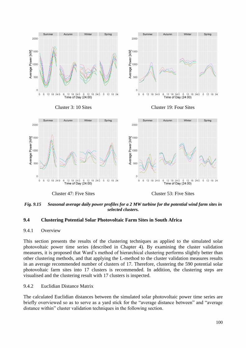
100

Cluster 3: 10 Sites

Cluster 19: Four Sites

Cluster 47: Five Sites

Cluster 53: Five Sites

Fig. 9.15 Seasonal average daily power profiles for a 2 MW turbine for the potential wind farm sites in

selected clusters.

9.4 Clustering Potential Solar Photovoltaic Farm Sites in South Africa

9.4.1 Overview

This section presents the results of the clustering techniques as applied to the simulated solar

photovoltaic power time series (described in Chapter 4). By examining the cluster validation

measures, it is proposed that Ward’s method of hierarchical clustering performs slightly better than

other clustering methods, and that applying the L-method to the cluster validation measures results

in an average recommended number of clusters of 17. Therefore, clustering the 590 potential solar

photovoltaic farm sites into 17 clusters is recommended. In addition, the clustering steps are

visualised and the clustering result with 17 clusters is inspected.

9.4.2 Euclidian Distance Matrix

The calculated Euclidian distances between the simulated solar photovoltaic power time series are

briefly overviewed so as to serve as a yard stick for the “average distance between” and “average

distance within” cluster validation techniques in the following section.

101

A subset of the Euclidian distance matrix for the solar photovoltaic time series can be seen in Table

9.3, where only the first five time series have been considered. It is necessary to keep in mind that

each time series ranges between 0 kW and 2000 kW, and that each time series has 70 080 records.

Table 9.3 Subset of the Euclidian distance matrix for the simulated solar photovoltaic time series. Time Series 1 2 3 4 5

1 0 25203.41 46493.63 39471.18 34951.21

2 25203.41 0 42110.49 42109.41 38779.19

3 46493.63 42110.49 0 54843.48 51816.6

4 39471.18 42109.41 54843.48 0 32334.84

5 34951.21 38779.19 51816.6 32334.84 0

A box and whisker diagram for the Euclidian distances between the simulated wind power time series

is given in Fig. 9.6. It can be seen that 50% of the Euclidian distances fall between approximately

54 000 and 66 000, with a median of approximately 78 000.

Fig. 9.16 Box and whisker diagram for the Euclidian distances between the simulated solar

photovoltaic power time series.


The results of the four cluster validation methods will now be presented. Fig. 9.17 presents the

average Euclidian distance between the clusters. It is expected that as the number of clusters increase,

the average distance between clusters decreases, although for a given number of clusters a higher

average distance between clusters is desirable. It can be seen that the complete-linkage and average-

linkage methods show a greater average distance between the clusters, outperforming Ward’s method

and the PAM clustering method. Ward’s method does show slightly higher distances between clusters

compared to the PAM method.

102


and different number of clusters in the solar photovoltaic power time series clustering procedure.

Fig. 9.18 presents the average Euclidian distance within the clusters. Ward’s method and the PAM

clustering method show similar results, with lower distances within clusters than the other methods,

which is desirable.


and different number of clusters in the solar photovoltaic power time series clustering procedure.

Fig. 9.19 presents the average silhouette widths of the time series associated with the respective

clusters. As stated before, the average silhouette width metric is a measure of the membership strength

of time series to their respective clusters, and is based on the pairwise difference of between and

within-cluster distances [94]. It results in a score between -1 and 1, where -1 one indicates a very poor

clustering and 1 represents a very good clustering. The results indicate that all the clustering methods

resulted in fairly average clustering results, with mixed results across the range of cluster numbers.

A higher average silhouette width score would require a greater difference between the between and

within-cluster distances, which is not a property of the simulated solar photovoltaic power time series

as all the time series are bound by the same range. It is seen, however, that as the number of clusters

increase, the average silhouette width decreases, which suggests using fewer clusters rather than more

clusters results in a better clustering.

103

Fig. 9.19 Comparison of average silhouette width for different clustering methods and different

number of clusters in the solar photovoltaic power time series clustering procedure.

Fig. 9.20 displays the result of the Caliński-Harabasz (CH) index. As stated before, the CH index

calculates the ratio between cohesion and separation, with a higher ratio being preferable. As the

number of clusters increases, the ratio between cohesion and separation deteriorates. At every given

number of clusters, Ward’s method and the PAM clustering method displays a higher CH index

compared to the other clustering methods.

Fig. 9.20 Comparison of Caliński-Harabasz (CH) index for different clustering methods and different

number of clusters in the solar photovoltaic power time series clustering procedure.

Ward’s method is the best performer in the average Euclidian distance within the clusters metric and

the Caliński-Harabasz index, and outperforms the PAM method at lower cluster numbers. It is

therefore henceforth the preferred clustering methodology for simulated solar photovoltaic power

time series. Similar to the wind power time series case, the choice of Ward’s method also makes sense

for the intended purpose of this clustering result (see end of section 9.3.3).

9.4.4 Visualisation of the Clustering Steps

Fig. 9.21 visualises the clustering steps for two to seven solar photovoltaic time series clusters using

Ward’s method of hierarchical clustering.

104

Two Clusters

Three Clusters

Four Clusters

Five Clusters

Six Clusters

Seven Clusters

Fig. 9.21 Visualisation of the clustering steps in the Ward’s method of hierarchical clustering for two

to seven simulated solar photovoltaic time series clusters.

105

When observing Fig. 9.11, the result of the hierarchical agglomerative (“bottom-up”) approach is

clear. At each clustering step, the cluster with the highest Ward’s distance between its respective time

series is split into a further two clusters.

Considering the case when two and three clusters are selected, it would seem that the biggest

differentiator between the solar photovoltaic simulations from different sites is the longitude of the

sites. This of course makes sense as it relates to irradiance profile in the different clusters, i.e. the

time of sunrise and sunset.

When four clusters are selected, the coastal region in KwaZulu Natal and the north-eastern part of the

Eastern Cape is separated into its own cluster. This is because of the lower capacity factors achieved

in this region, as can be seen in Fig. 9.4. This region of South Africa has a sub-tropical climate [102]

that is characterised by high levels of cloud cover and frequent rains during the summer months,

leading to a lower solar-photovoltaic energy yield.

When five and six clusters are selected, the coastal zones and areas bordering the coastal zones are

separated from those areas further inland, mainly due to the difference in solar irradiance between

these respective areas that is again caused by differences in cloud cover.

Specifying seven clusters separates the north-eastern cluster into two separate clusters.

9.4.5 Appropriate Number of Clusters

The simulated solar photovoltaic time series displayed much lower Euclidian distances between the

respective time series than in the case of wind power simulations, leading to much lower average

centroid errors. As such, it is decided that the L-method will be applied to all four cluster validation

methods (as applied to the result obtained using Ward’s method of hierarchical clustering), in order

to determine the appropriate number of clusters.

It can be seen in Fig. 9.22 how the L-method is applied to one of the cluster validation measures,

namely the average Euclidian distance between the clusters, in order to find a point, 𝑐, where the total

root-mean-squared error (RMSE) of the left and right linear models are minimised. For this cluster

validation measure, using 19 clusters minimises the total RMSE.

Fig. 9.22 Visualisation of the L-method applied to the average Euclidian distance between clusters

using Ward’s method of hierarchical clustering. The point c is found to be 19 for this cluster validation

measure.

106

Table 9.4 shows the results of the L-method as applied to all of the cluster validation measures under

consideration. The average result of the L-method applied to all the cluster validation measures gives

the point, 𝑐, as 17. It is therefore proposed that 17 clusters be used for the simulated solar-photovoltaic

power time series.

Table 9.4 Results of the L-method Applied to Different Cluster Validation Measures Cluster Validation Measure Point c obtained from the L-method

Average Euclidian distance between clusters 19

Average Euclidian distance within clusters 20

Average Silhouette Width 8

Caliński-Harabasz Index 21

9.4.6 Inspection of the Optimal Clustering Result

The spatial distribution of the optimal simulated solar photovoltaic power time series clustering result,

using Ward’s method of hierarchical clustering for 17 clusters, can be seen in Fig. 9.23.

Fig. 9.23 Spatial distribution of solar photovoltaic site clusters obtained using Ward’s method for 17

clusters.

The average seasonal daily power profiles of a selection of different clusters are inspected in Fig.

9.24. In Fig. 9.24, summer is defined as December to February, autumn is defined as March to May,

winter is defined as June to August and spring is defined as September to November.

Cluster 1 (Limpopo region) and cluster 13 (north-east Western Cape region) have been included to

showcase the difference between two clusters. The seasonal daily average profiles of the simulated

107

solar photovoltaic power time series of both clusters reach similar maximum power outputs during

winter, although this represents the strongest power output season for cluster 1 and the weakest power

output season for cluster 13. There is also a time shift, with cluster 1 starting power delivery earlier

in the day than cluster 13.

Cluster 1: 53 Sites

Cluster 13: 30 Sites

Fig. 9.24 Seasonal average daily power profiles for a 2 MW solar photovoltaic installation for the

potential solar photovoltaic farm sites in selected clusters.

108

9.5 Case Study 1: Different Formulations of Mean-variance Optimisation

9.5.1 Overview

In the literature, mean-variance portfolio theory has been applied to minimise the variance of wind

power. This case study examines the effect of including the solar photovoltaic power time series and

the load time series in the optimisation procedure.

The size of the case study is arbitrarily chosen to represent the wind and solar capacities assigned in

the IRP 2010 policy document for the year 2030 (see section 2.2.1). Therefore the optimal allocation

of 9 200 MW of wind farm capacity and 8 400 MW of solar photovoltaic farm capacity will be

considered. It is assumed that the load in 2030 will be the same as in peak load year, 2007. Four

scenarios are studied, as summarised in Table 9.5.

Table 9.5 Summary of the four scenarios studied in case study 1. Scenario Data Included in Optimisation Optimisation Target Mathematical

formulation

1 Simulated wind power time series Minimise variance of cumulative

wind power output

Section 5.3.

2 Simulated wind power time series and load

time series

Minimise variance of load minus

wind power output

Section 5.5

(excluding solar).

3 Simulated wind power time series and

simulated solar photovoltaic time series

Minimise variance of cumulative

renewable power output

Section 5.4.

4 Simulated wind power time series, simulated

solar photovoltaic time series and load time

series

Minimise variance of residual load Section 5.5.

In case study 1, the clustering techniques that have been applied in section 9.3 and section 9.4 are

used to cluster the simulated wind time series and simulated solar photovoltaic time series. For each

resulting cluster a centroid time series is calculated that is used as an input to the mean variance

optimisation procedure. The effect of the time series clustering and the justification of its use are

examined in case study 2.

In scenarios 1 and 2, it is assumed that the full 8 400 MW of solar photovoltaic capacity is added to

the system. An average time series of all the photovoltaic time series is used to achieve this. In case

studies 3 and 4, the solar photovoltaic capacity is allocated by the optimisation procedure.

9.5.2 Mean-Variance Variable Assumptions

All the variable assumptions that are made in case study 1 are shown in Table 9.6.

109

Table 9.6 Summary of Variable Assumptions in case study 1. Variable Meaning Value

𝜇Min Desired Solar The minimum overall mean solar photovoltaic

power output (related to capacity factor)

Not set

𝑤Total Wind The total wind farm capacity that is to be allocated. 9 200 MW

𝑤Max Total Solar The maximum solar photovoltaic farm capacity

that can be allocated.

8 400 MW

max𝑥, 𝑥 ∈ Wind Maximum wind farm capacity that can be assigned

to each 27 x 31 km site.

500 MW

max𝑥, 𝑥 ∈ Solar Maximum wind farm capacity that can be assigned


1 000 MW

The 𝜇Min Desired Solar variable is not set in this case study. It is only necessary when there are sites

with very low solar photovoltaic power outputs that need to be limited. The capacity constraints per

site, max𝑥, represent conservative estimates of how much capacity could be built on a single potential

wind farm site or solar photovoltaic farm site.

9.5.3 Scenario Efficient Frontiers

The efficient frontiers of each scenario will now be inspected. The efficient frontier shows the

minimised target and is obtained by solving the optimisation problem for a range of different values

of 𝜇Desired Wind , the desired mean wind power output, which can be transformed to wind farm

capacity factor by dividing by the total wind farm capacity (9 200 MW in case study 1).

9.5.3.1 Scenario 1 Efficient Frontier

The efficient frontier for scenario 1 is shown in Fig. 9.25. The minimisation target, the variance of

cumulative wind power output, is plotted on the y-axis and the capacity factor (𝜇Desired Wind) is

plotted on the x-axis.

Fig. 9.25 Efficient frontier of scenario 1.



load minus wind power output, is plotted on the y-axis and the capacity factor (𝜇Desired Wind) is


110




cumulative renewable power output, is plotted on the y-axis and the capacity factor (𝜇Desired Wind) is



Unlike scenarios 1 and 2, where 8 400 MW of solar photovoltaic capacity was uniformly allocated,

the mean-variance optimisation procedure determined the allocation (and therefore the total solar

capacity), for every value of 𝜇Desired Wind , that would minimise the variance of the cumulative

renewable power output. This can be seen in Fig. 9.28. The totals are relatively low when compared

to the 9 200 MW of wind farm capacity that is added.

111

Fig. 9.28 Solar photovoltaic capacity included in efficient frontier solutions of scenario 3.



residual load, is plotted on the y-axis and the capacity factor (𝜇Desired Wind) is plotted on the x-axis.


Unlike scenarios 1 and 2, where 8 400 MW of solar photovoltaic capacity was uniformly allocated,

the mean-variance optimisation procedure determined the allocation (and therefore the total solar

capacity), for every value of 𝜇Desired Wind, that would minimise the variance of the residual load. This

can be seen in Fig. 9.30. A higher overall wind farm capacity factor required a higher capacity of

solar photovoltaic farm capacity. Also, the solar photovoltaic farm capacities are considerably higher

than those assigned in scenario 3 (in the order of 900 to 1 400 MW).

112

Fig. 9.30 Solar photovoltaic capacity included in efficient frontier solutions of scenario 4.

9.5.4 Comparison of Scenario Performance

The four scenarios will now be compared using the standard deviation of the renewable power output

and the standard deviation of the residual load. Fig. 9.31 displays the standard deviations of the

renewable power output of the efficient frontier solutions of scenarios 1 to 4. It is important to

remember that scenarios 1 and 2 both have 8 400 MW of uniformly distributed solar photovoltaic

capacity, while scenario 3 has solar photovoltaic capacity in the order of 900 MW to 1 400 MW and

scenario 4 has solar photovoltaic capacity in the order of 5 000 MW to 5 700 MW. Predictably, it is

scenario 3 that has the lowest standard deviation of renewable power output as this was its

optimisation goal.

Fig. 9.31 Standard deviations of renewable power outputs of efficient frontier solutions of scenarios 1-

4.

The standard deviation of the residual load is arguably of more importance than the standard deviation

of the renewable power output, and is shown in Fig. 9.32. Also plotted on Fig. 9.32, is the standard

deviation of the current load, i.e. the load time series before any renewable power has been subtracted

(with its annual and seasonal trends removed). It is telling that at this level of wind power capacity

addition, the standard deviation of the load can actually be reduced significantly if the right

optimisation procedure is used to allocate wind farm capacity and solar photovoltaic farm capacity.

113

It is also possible to see that the solutions obtained in scenario 3 does not in fact reduce the standard

deviation of the residual load, meaning that minimising the variance of renewable power output while

excluding the load time series data from the optimisation procedure will lead to sub-optimal results.

This is mainly due to the low solar allocation in scenario 3, which ignores the correlation that solar

photovoltaic power has with the rise and fall of the daily load profile.

Fig. 9.32 Standard deviations of residual loads of efficient frontier solutions of scenarios 1-4.

9.5.5 Comparison of all Scenario Solutions at 40% Wind Farm Capacity Factor

Every point on the efficient frontier represents a solution which consists of a particular distribution

of wind farm and solar photovoltaic farm capacity. The solutions that fall at the 40% wind farm

capacity factor level of every efficient frontier for scenarios 1 to 4 is now inspected. The solution at

40% wind farm capacity factor is chosen because it represents a solution with a high wind energy

yield, but falls at a point where the minimisation target is still relatively close to its absolute minimum.

Fig. 9.33 shows the spatial distribution of the 9 200 MW of wind farm capacity that is allocated in

the 40% wind power capacity factor solution in each scenario. There are similarities between

scenarios 1 and 3, where the load time series has not been taken into account. The same can be said

for scenarios 2 and 4, where the load time series is taken into account.

114

Scenario 1

Scenario 2

Scenario 3

Scenario 4

Fig. 9.33 Spatial distributions of the 9 200 MW of wind farm capacity of 40% wind farm capacity

factor solutions on the efficient frontiers of scenarios 1-4.

Fig. 9.34 shows the size and spatial distribution of the solar photovoltaic farm capacity that is present

in the 40% wind power capacity factor solution of each scenario. As stated before, a uniform

distribution of solar photovoltaic capacity is assumed in scenarios 1 and 2 (note that each site is

assigned 14.24 MW, even though this is rounded to 14 MW in Fig. 9.34). The difference between the

solar photovoltaic capacity allocation in scenarios 3 and 4 is also clear. Scenario 4 shows that

including the load into the optimisation procedure significantly increases the solar photovoltaic

capacity, but to the level of 8 400 MW as mandated in the IRP 2011 policy document. The solar

photovoltaic capacity in scenario 4 is also mainly allocated in the south-west of the country, possibly

as a result of the solar photovoltaic profiles of this region playing a bigger role in meeting the peak

load, which stems mainly from the load centres in the north east of the country.

115

Scenario 1: 8 400 MW




Fig. 9.34 Size and spatial distributions of the solar photovoltaic farm capacity of the 40% wind farm

capacity factor solutions on the efficient frontiers of scenarios 1-4.

Fig. 9.35 shows the seasonal average daily power profiles for the renewable power output of the 40%

wind farm capacity factor solutions on the efficient frontiers of scenario 1 to 4. From Fig. 9.35 it is

clear that scenario 3 minimises the variance of the renewable power output. Also, the seasonal average

power profiles of scenarios 1 and 2 look quite similar (both are dominated by the relatively large solar

photovoltaic capacity), but we have already seen from Fig. 9.32 that the standard deviation of the

residual load in these two cases differ substantially. This could point to the dangers of using daily

average profiles for analysis. Scenario 4 results in the “widest” daily power profiles, which optimally

covers the load.

116

Scenario 1

Scenario 2

Scenario 3

Scenario 4

Fig. 9.35 Seasonal average daily power profiles for the renewable power output of the 40% wind farm

capacity factor solutions on the efficient frontiers of scenarios 1-4.

9.5.6 Inspection of Scenario 4 solution at 40% Wind Farm Capacity Factor

In section 9.5.4 it was shown that including the wind power time series, solar photovoltaic power

time series and load in the optimisation procedure (as in scenario 4), could actually result in a residual

load with a lower standard deviation than the original load time series. The scenario 4 solution at 40%

wind farm capacity factor is now investigated further.

Fig. 9.36 shows the seasonal average daily wind power profiles for the wind power output of the 40%

wind farm capacity factor solution of scenario 4. It can be seen that there is considerably more

variance in the wind power output during autumn and winter than during summer and spring. It is

hypothesised that this is a characteristic of the wind resource in South Africa. This characteristic will

have an effect on the power system as will be shown in the following figures.

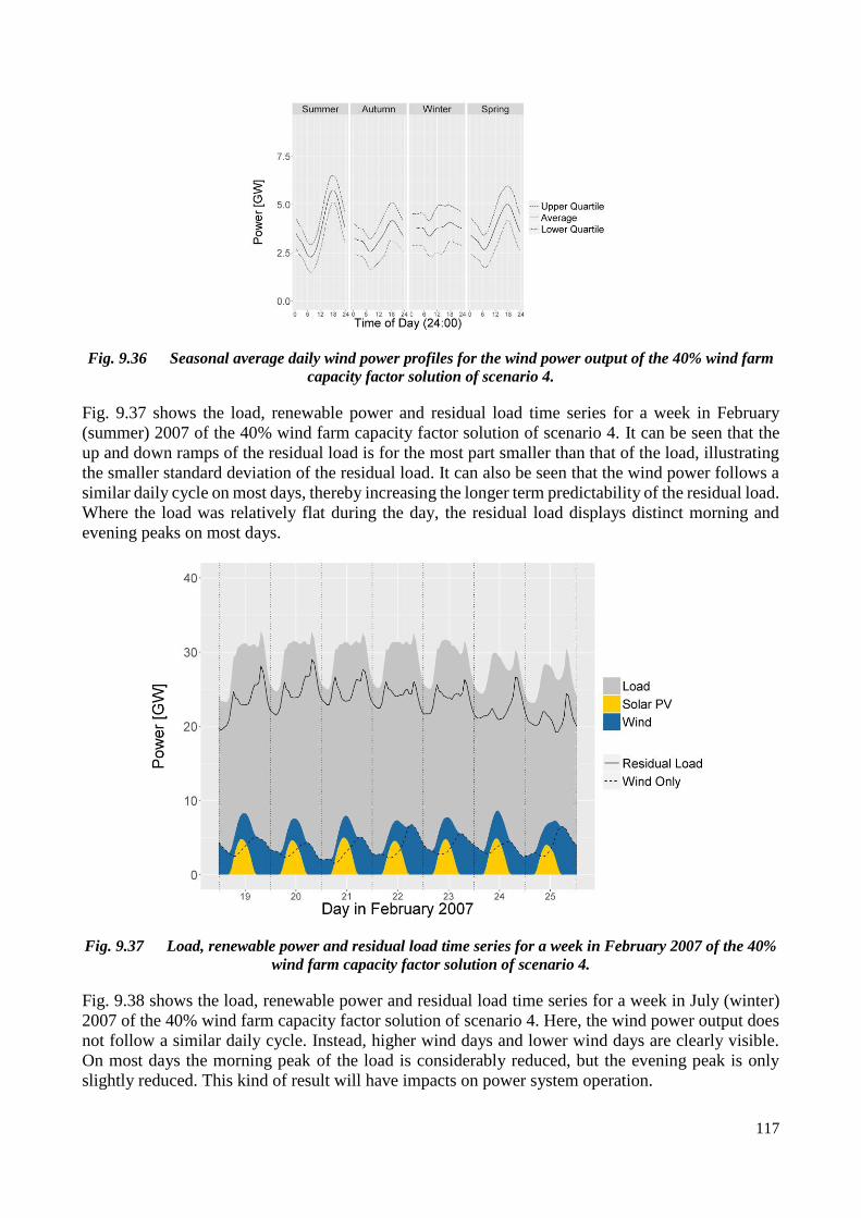
117

Fig. 9.36 Seasonal average daily wind power profiles for the wind power output of the 40% wind farm

capacity factor solution of scenario 4.

Fig. 9.37 shows the load, renewable power and residual load time series for a week in February

(summer) 2007 of the 40% wind farm capacity factor solution of scenario 4. It can be seen that the

up and down ramps of the residual load is for the most part smaller than that of the load, illustrating

the smaller standard deviation of the residual load. It can also be seen that the wind power follows a

similar daily cycle on most days, thereby increasing the longer term predictability of the residual load.

Where the load was relatively flat during the day, the residual load displays distinct morning and

evening peaks on most days.

Fig. 9.37 Load, renewable power and residual load time series for a week in February 2007 of the 40%

wind farm capacity factor solution of scenario 4.

Fig. 9.38 shows the load, renewable power and residual load time series for a week in July (winter)

2007 of the 40% wind farm capacity factor solution of scenario 4. Here, the wind power output does

not follow a similar daily cycle. Instead, higher wind days and lower wind days are clearly visible.

On most days the morning peak of the load is considerably reduced, but the evening peak is only

slightly reduced. This kind of result will have impacts on power system operation.

118

Fig. 9.38 Load, renewable power and residual load time series for a week in July 2007 of the 40% wind

farm capacity factor solution of scenario 4.

119

9.6 Case Study 2: REIPPPP Round 1-3 vs. Optimisation (Unclustered and Clustered)

9.6.1 Overview

This case study compares the optimisation procedure (considering wind power, solar photovoltaic

power and load) with the wind farm and solar photovoltaic farm allocation in the REIPPPP, in order

to quantify the benefits of the optimisation procedure when compared with a real-world allocation in

South Africa. This case study also justifies the use of time series clustering by examining the effect

that time series clustering has on the results of the optimisation procedure when compared to the

unclustered optimisation as found in the literature.

Wind power simulations were performed for all the wind farm projects in rounds 1 to 3 of the

REIPPPP, excluding two wind farms at De Aar in the Northern Cape due to their location falling

outside the WASA wind dataset. Therefore, a total of 1 778 MW of wind farm capacity is considered.

The method used to simulate the wind power time series is exactly the same as the method described

in section 3.2. In each case, the WASA wind speed time series closest to the respective REIPPPP

wind farm was used to perform the simulation, using a wind turbine power curve that matches the

actual wind turbine power curve. The details of the wind farms that were considered in this case study

is given in Table 9.7. The wind turbine power curves that were used for the REIPPPP simulation is

shown in Fig. 9.39.

Solar photovoltaic simulations were also done for the solar photovoltaic projects in rounds 1 to 3 of

the REIPPPP. Therefore, a total of 1 484 MW of solar photovoltaic farm capacity is considered. The

method used to simulate the solar photovoltaic power time series is exactly the same as the method

described in section 3.3. In each case, the SoDa irradiance and temperature time series closest to the

respective REIPPPP solar photovoltaic farm was used to perform the simulation, assuming a fixed

angle installation (i.e. no tracking). The details of the solar photovoltaic farms that were considered

in this case study are given in Table 9.8.

120

Table 9.7 Details of the Wind Farm Projects in REIPPPP Rounds 1-3 (excluding two wind farms at

De Aar in the Northern Cape). Name REIPPPP

Phase

Provinc

e

Capacity

(MW)

Turbine

Model

Hub

Height

(m)

Turbine

Rated

Power

(MW)

Number

of

Turbines

Latitude Longitude

Cookhouse Wind

Farm

1 Eastern

Cape

138.6 Suzlon S88 2.1

MW

80 2.1 66 -32.81 25.91

Dorper Wind Farm 1 Eastern

Cape

100 Nordex N100

2.5MW

80 2.5 40 -31.48 26.45

Jeffreys Bay Wind

Farm

1 Eastern

Cape

138 Siemens SWT-

2.3-108

80 2.3 60 -34.00 24.84

Kouga Wind Farm 1 Eastern

Cape

80 Nordex N90

2.5 MW

80 2.5 32 -34.15 24.72

Metrowind Van

Stadens Wind Farm

1 Eastern

Cape

27 Sinovel

SL3000-113

90 3 9 -33.96 25.24

Noblesfontein

Gestamp Wind

Farm

1 Northern

Cape

73.8 Vestas V100

1.8MW

95 1.8 41 -31.70 23.18

Dassiesklip Wind

Energy Facility

1 Western

Cape

27 Sinovel

SL3000-113

100 3 9 -34.23 19.38

Hopefield Umoya

Wind Farm

1 Western

Cape

66.6 Vestas V100

1.8MW

95 1.8 37 -33.10 18.40

Amakhala Emoyeni

Wind Farm

2 Eastern

Cape

134.4 Nordex N117

2.4MW

91 2.4 56 -32.75 25.93

Chaba Wind Farm 2 Eastern

Cape

21 Vestas V112

3MW

84 3.075 7 -32.59 27.34

Grassridge Wind

Project

2 Eastern

Cape

61.5 Vestas V112

3MW

84 3.075 20 -33.65 25.59

Tsitsikamma

Community Wind

Farm

2 Eastern

Cape

95 Vestas V112

3MW

94 3.075 31 -34.08 24.50

Waainek Wind

Project

2 Eastern

Cape

24.6 Vestas V112

3MW

84 3.075 8 -33.33 26.47

Gouda Wind

Facility

2 Western

Cape

138 Acciona AW-

100-3000

100 3 46 -33.26 19.03

West Coast One

Wind Farm

2 Western

Cape

94 Vestas V90

2MW

80 2 47 -32.83 18.00

Gibson Bay Wind

Farm

3 Eastern

Cape

110 Nordex N117

3MW

91 3 37 -34.14 24.52

Nojoli Wind Farm 3 Eastern

Cape

88 Vestas V100

2MW

80 2 44 -32.77 25.92

Khobab Wind Farm 3 Northern

Cape

140 Siemens SWT-

2.3-108

99.5 2.3 61 -30.43 19.49

Loeriesfontein 2

Wind Farm

3 Northern

Cape

140 Siemens SWT-

2.3-108

99.5 2.3 61 -30.40 19.60

Noupoort Wind

Farm

3 Northern

Cape

80.5 Siemens SWT-

2.3-108

99.5 2.3 35 -31.18 25.05

Fig. 9.39 Wind turbine power curves used in the REIPPPP simulation

0

500

1000

1500

2000

2500

3000

3500

0 1 2 3 4 5 6 7 8 9 10 11 12 13 14 15 16 17 18 19 20 21 22 23 24 25 26 27 28 29

Pow

er [

kW

]

Wind Speed [m\s]

Vestas V100 2MW

Siemens SWT-2.3-108

Suzlon S88 2.1 MW

Nordex N100 2.5MW

Nordex N90 2.5 MW

Vestas V100 1.8MW

Sinovel SL3000-113

Acciona AW-100-3000

Nordex N117 2.4MW

Vestas V112 3MW

Vestas V90 2MW

UP500-86

Nordex N117 3MW

121

Table 9.8 Details of the Solar Photovoltaic Farm Projects in REIPPPP Rounds 1-3. Name REIPPPP

Phase

Province Capacity

(MW)

Longitude Latitude

Letsatsi Power Company 1 Free State 64 25.92 -28.92

Soutpan Solar Park 1 Limpopo 28 29.25 -22.99

Witkop Solar Park 1 Limpopo 30 29.36 -24.04

RustMo1 Solar Farm 1 North West 6.76 27.42 -25.74

Aries Solar PV Energy Facility 1 Northern Cape 9.65 20.79 -29.50

De Aar Solar PV 1 Northern Cape 48.25 24.03 -30.62

Droogfontein Solar PV Project 1 Northern Cape 48.25 24.76 -28.61

Greefspan PV Power Plant 1 Northern Cape 10 23.31 -29.39

Herbert PV Power Plant 1 Northern Cape 19.9 23.80 -29.00

Kalkbult 1 Northern Cape 72.5 24.14 -30.16

Kathu Solar Energy Facility 1 Northern Cape 75 23.03 -27.61

Konkoonsies Solar 1 Northern Cape 9.65 19.56 -28.89

Lesedi Power Company 1 Northern Cape 64 23.37 -28.31

Mulilo Renewable Energy Solar PV De Aar 1 Northern Cape 9.65 24.01 -30.63

Mulilo Renewable Energy Solar PV Prieska 1 Northern Cape 19.9 22.32 -29.97

Solar Capital De Aar 1 Northern Cape 75 24.10 -30.60

SlimSun Swartland Solar Park 1 Western Cape 5 18.53 -33.35

Touwsrivier CPV Solar Project 1 Western Cape 36 19.93 -33.41

Project Dreunberg 2 Eastern Cape 69.9 26.21 -30.83

Boshoff Solar Park 2 Free State 60 25.19 -28.46

Jasper Power Company 2 Northern Cape 75 23.35 -28.32

Linde Solar Project 2 Northern Cape 36.8 24.66 -31.00

Sishen Solar Facility 2 Northern Cape 74 22.93 -27.58

Solar Capital De Aar 3 2 Northern Cape 75 24.10 -30.60

Upington Solar PV 2 Northern Cape 8.9 21.27 -28.40

Aurora Solar Project 2 Western Cape 9 18.50 -32.64

Vredendal Solar Power Park 2 Western Cape 8.8 18.51 -31.63

Pulida Solar Park 3 Free State 75 24.90 -29.09

Tom Burke Solar Park 3 Limpopo 60 27.99 -23.07

Adams Solar PV 2 3 Northern Cape 75 23.01 -27.38

Mulilo Prieska PV 3 Northern Cape 75 22.32 -30.04

Mulilo Sonnedix Prieska PV 3 Northern Cape 75 22.36 -30.02

Paleisheuwel Solar PV Park 3 Western Cape 75 18.73 -32.42

Case study 2 compares three different distributions of renewable energy capacity as can be seen in

Table 9.9. Both an unclustered and clustered optimisation is performed. This is done to justify the use

of the clustering procedure, as the unclustered optimisation yields slightly better results, but fails to

provide practicable solutions. The unclustered optimisation considers all the simulated power time

series (402 wind power time series from the Vestas 2 MW platform and 590 solar photovoltaic time

series). The clustered optimisation considers the centroid time series that were calculated using the

preferred clustering methodology and appropriate numbers of clusters as discussed in sections 9.3

and 9.4.

122

Table 9.9 Three distributions that are compared in case study 2. Distribution Name Distribution Details

REIPPPP Distributions obtained from REIPPPP

Optimised Unclustered Distributions allocated by the mean-variance optimisation procedure

considering all individual wind and solar photovoltaic time series and load

Optimised Clustered Distributions allocated by the mean-variance optimisation procedure

considering centroid wind and solar photovoltaic time series (calculated using

the time series clustering methodology) and load



Table 9.10 Summary of variable assumptions in case study 2. Variable Meaning Value



Not set




1 484 MW



500 MW



1 000 MW





9.6.3 Efficient Frontiers

As stated before, the efficient frontiers display the minimisation target on the y-axis and the desired

wind farm capacity factor on the x-axis. The efficient frontier for the minimised standard deviation

(variance) of residual load of the unclustered and clustered optimisation procedures are shown in Fig.

9.40, as well as the standard deviation of the residual load from the REIPPPP distribution. It can be

seen that the unclustered and clustered optimisations performed similarly across the range of desired

wind farm capacity factors, with the unclustered optimisation expectedly performing slightly better

(achieving a lower standard deviation of residual load). Although the standard deviation of the

residual load of the REIPPPP distribution is lower than the standard deviation of the current load,

both the optimisations succeed in achieving a significantly lower standard deviation. It is also clear

that there is scope for an increased wind farm capacity factor when comparing the REIPPPP

distribution with the optimisation results.

123

Fig. 9.40 Efficient frontiers of the unclustered and clustered optimisation procedures, as well as the

standard deviation of the REIPPPP distribution’s residual load.

9.6.4 Comparison of Unclustered and Clustered Solutions at 40% Wind Farm Capacity Factor

with REIPPPP

The solutions at 40% wind farm capacity factor will now be compared with the REIPPPP distribution.

In Fig. 9.41, the distribution of wind farm capacity in REIPPPP rounds 1 to 3 is shown.

Fig. 9.41 Wind Farm distribution in REIPPPP Rounds 1-3 (excluding two wind farms at De Aar in the

Northern Cape).

124

Fig. 9.42 shows the spatial distribution of the wind farm capacity of the solution at 40% wind farm

capacity factor of the unclustered solution. Low capacities are allocated to certain sites, which makes

part of the solution unfeasible in the face of practical and economic considerations. The capacities

are furthermore assigned to exact coordinates, yielding a very rigid solution when factors such as land

use, grid connection capacity, etc. have not been taken into account. There is no clear site selection

alternatives should a specific site be disqualified based on these considerations.

Fig. 9.42 Wind Farm distribution of 1 778 MW of the solution at 40% wind farm capacity factor in the

unclustered optimisation.

Fig. 9.43 shows the spatial distribution of the wind farm capacity of the solution at 40% wind farm

capacity factor of the clustered solution. As has been confirmed by respective efficient frontiers, the

performance of the unclustered and clustered solution is comparable, but the clustered solution is

more feasible as it provides a broader range of options to implement the solutions. The capacities are

allocated to geographical areas with similar wind power profiles rather than individual potential wind

farm sites. The same phenomenon holds true for the solar photovoltaic capacity distribution, which

is not shown here. Another consideration is that the unclustered optimisation procedure necessarily

contains many more time series and requires more time and memory to solve the optimisation on a

standard computer.

125

Fig. 9.43 Wind Farm distribution of 1 778 MW of the solution at 40% wind farm capacity factor in the

clustered optimisation.

Fig. 9.44 displays a week of load and the residual loads stemming from the clustered solution (at 40%

wind farm capacity factor) and the REIPPPP distribution. It serves as an example of the impact of the

optimisation procedure. Even at this relatively low penetration of renewable power capacity, it can

be seen that the evening peaks are generally much lower with the clustered optimised solution, in the

order of 1 000 MW lower than the load, and 500 MW lower than the REIPPPP distribution (on most

days).

Fig. 9.44 Load and residual load time series from the clustered solution (at 40% wind farm capacity

factor) and the REIPPPP distribution for a week in February 2007.

126

9.7 Case Study 3: Optimal Future Penetrations of Wind and Solar Photovoltaic Power

Capacity in South Africa

9.7.1 Overview

This case study uses the mean-variance optimisation procedure to allocate a range of future

penetrations of wind power capacity with complementing solar photovoltaic power capacity in South

Africa, in order to study the effect that increasing penetrations of renewable energy will have on the

conventional generation capacity requirements and to determine an optimal ratio of wind power

capacity to solar photovoltaic power capacity.

Similar to case study 1, and unlike case study 2, the constraint that controls the maximum total solar

photovoltaic capacity is not set in this case study. This allows the optimisation procedure to allocate

as much solar photovoltaic capacity to the specified wind farm capacity in order to minimise the

variance of the residual load. This will result in different ratios of solar photovoltaic power capacity

to wind power capacity as the wind power capacity increases.

In order to study the effect that increasing penetrations of renewable energy will have on the power

system, this case study employs two of the key performance indicators that have not been used before,

namely the capacity credit and the generator capacity by type metric.

This case study ignores the existing and planned wind and solar farm capacity in the REIPPPP and

assumes the optimisation procedure was used from the beginning to allocate the renewable power

capacity. In a real-life study to plan an exact future solution, the existing REIPPPP capacity could be

incorporated in the optimisation procedure in the same manner that the load data has been

incorporated, i.e. included and constrained with a weight of one. This would result in new capacity

complementing the existing capacity in terms of reducing the variance of the existing load. However,

the REIPPPP capacity is still sufficiently small, so it is ignored in this case study.

The same load data, which effectively describes the peak load year of 2007 (as discussed in section

7.5), is used for every penetration level of wind power capacity with complementing solar

photovoltaic power capacity. This is of course unrealistic, as the load will likely change as future

wind and solar photovoltaic power capacity is added to the grid over time. However, it has been kept

constant here in order to isolate the effect of increasing renewable power capacities.






Not set

𝑤Total Wind The total wind farm capacity that is to be allocated. 1 000 MW to 30 000 MW



Not set



500 MW



1 000 MW

127





9.7.3 Optimal Future Penetrations of Wind and Solar Photovoltaic Power

Fig. 9.45 shows the minimised standard deviations of residual load for different penetrations of wind

farm capacity with complementing solar photovoltaic power (at different wind farm capacity factors).

On the x-axis, the amount of complementing solar photovoltaic power capacity is also indicated,

starting at 4.7 GW of solar photovoltaic capacity for 2 GW of wind power capacity and ending at

7.9 GW of solar photovoltaic capacity for 30 GW of wind power capacity. It is clear from Fig. 9.45

that solutions from 35% wind farm capacity factor to 40% wind farm capacity factor display similar

results in terms of the standard deviation of residual load across the range of installed wind farm

capacities, while opting for a higher wind farm capacity factor solution (41% to 45%) drastically

increases the standard deviation of residual load at wind power penetrations above approximately

6 GW. It is also clear that the standard deviation of the current load can be reduced by installing

renewable power capacity up to a point depending on the wind farm capacity factor of the solution,

e.g. at 40% wind farm capacity factor, approximately 14 GW of wind power capacity with

approximately 6.2 GW of solar photovoltaic power capacity can be installed before the standard

deviation of the residual load increases above the levels of the current load (this solution is inspected

further in case study 4). The standard deviation of the residual load is of course not the only factor to

consider when considering power system design, e.g. the residual load with 14 GW of wind power

capacity with approximately 6.2 GW of solar photovoltaic power capacity will almost certainly lose

the long term predictability of the current load, even though it has a similar standard deviation as the

current load.

Fig. 9.45 Optimised standard deviations of residual load for different penetrations of wind farm

capacity with complementing solar photovoltaic power (at different wind farm capacity factors).

Fig. 9.46 shows the optimal ratios of solar photovoltaic farm capacity to wind farm capacity for

different penetrations of wind farm capacity (as a percentage of the total installed renewable power

128

capacity). This effectively plots the two x-axes on Fig. 9.45 against each other. Initially, solar

photovoltaic power is preferred because of its correlation with the daily load profile, but at some point

adding more solar photovoltaic power only serves to increase the standard deviation of the residual

load. This result points to the need for adequate storage capacity in the future if solar photovoltaic

power is to play a bigger role in meeting the load. It is clear from Fig. 9.46 that the solar photovoltaic

ratio is fairly independent from the wind farm capacity factor, meaning that the solar photovoltaic

ratio depends almost entirely on the nameplate capacity of the installed wind farms.

Fig. 9.46 Optimal ratios of solar photovoltaic farm capacity to wind farm capacity for different

penetrations of wind farm capacity (at different wind farm capacity factors).

9.7.4 Results of Key Performance Indicators

The capacity credit and the generator capacity by type metric are inspected for optimal future

penetrations of wind and solar photovoltaic power.

9.7.4.1 Capacity Credit

The Garver approximation of capacity credit (discussed in section 6.4) is shown in Fig. 9.47. It is

clear that the capacity credit is quite low at the lower penetrations of renewable power, mainly due to

the high share of solar photovoltaic capacity that is allocated by the optimisation procedure. The

capacity credit increases up until approximately 14 GW of wind farm capacity is installed (with

approximately 6.2 GW of solar photovoltaic capacity), after which it slowly decreases as the

renewable power capacity increases. It is also clear that the solutions with an extremely high wind

farm capacity factor (43% and above) experiences a steeper decrease in capacity credit. This is mainly

because specifying such a high wind farm capacity factor limits the options of the optimisation

procedure in terms of which clusters it can include in the solution, resulting in most of the allocated

capacity being assigned to relatively few clusters with high wind farm capacity factors in order to

meet the capacity factor constraint, thereby drastically increasing the intermittency of the wind power,

which makes it less reliable. The capacity credit approximation thus estimates the capacity credit of

129

the renewable power portfolio to peak at around 25–28% at about 14 GW of wind farm capacity and

6.2 GW solar photovoltaic farm capacity.

Fig. 9.47 The Garver capacity credit (left) and the Garver 5% highest load capacity credit (right)

approximations for optimal future penetrations of wind and solar photovoltaic power capacity

In Fig. 9.47 it can be seen that the solutions at 45% wind farm capacity factor stop at approximately

25 GW. This is simply where the optimisation procedure runs into all the cluster capacity constraints

(max𝑥 , 𝑥 ∈ Wind). There exist no solutions at higher penetrations of installed wind farms as the

clusters that satisfy the capacity factor constraints have been filled to capacity.

9.7.4.2 Generator Capacity by Type Metric

The results of the generator capacity by type metric is shown in Fig. 9.48 to Fig. 9.51. In Fig. 9.48,

the peaker capacity that is required to meet the residual load is shown for the optimal future

penetrations of wind and solar photovoltaic solar power capacity. The current peaker capacity

requirement is also indicated (which is obtained by applying the generator capacity by type metric to

the load data without any renewable power capacity). The peaker capacity is considerably higher than

the current peaker requirement even at low wind farm capacities, mainly due to the high initial solar

photovoltaic capacity. The solar photovoltaic capacity typically displaces load-following capacity in

favour of peaker capacity, because where load-following capacity would have been used throughout

the day the solar photovoltaic power now covers the load during morning, midday and afternoon but

requires peaker capacity for the early morning and late evening peak load periods. It is interesting to

note that the peak capacity requirement does not really increase even as renewable power capacity

increases.

130

Fig. 9.48 Peaker capacity requirement for optimal future penetrations of wind and solar photovoltaic

capacity.

In Fig. 9.49, the load-following capacity that is required to meet the residual load is shown for the

optimal future penetrations of wind and solar photovoltaic solar power capacity, with the current load-

following capacity requirement also being indicated. It is clear that an increase in renewable power

capacity at these optimal ratios of wind and solar photovoltaic power mainly leads to an increased

need for load-following capacity to meet the residual load. At 40% wind farm capacity factor, one

could install up to approximately 13 GW of wind farm capacity (with approximately 6.05 GW of

solar photovoltaic capacity) before additional load following capacity would be required as compared

to the required load following capacity to meet the current load.

Fig. 9.49 Load-following capacity requirement for optimal future penetrations of wind and solar

photovoltaic capacity.

In Fig. 9.50, the base-load capacity that is required to meet the residual load is shown for the optimal

future penetrations of wind and solar photovoltaic solar power capacity, with the current base-load

capacity requirement also being indicated. It is clear that an increase in renewable power capacity at

131

these optimal ratios of wind and solar photovoltaic power mainly leads to a decreased need for base-

load capacity to meet the residual load.

Fig. 9.50 Base-load capacity requirement for optimal future penetrations of wind and solar

photovoltaic capacity.

In Fig. 9.51, the total conventional capacity that is required to meet the residual load is shown for the

optimal future penetrations of wind and solar photovoltaic solar power capacity, with the current total

conventional capacity requirement also being indicated. This provides a general overview of the rate

at which the need for conventional generation capacity decreases at the renewable power capacity

increases.

Fig. 9.51 Total capacity requirement for optimal future penetrations of wind and solar photovoltaic

capacity.

It is important to remember that the capacity generator by type metric is a high level statistical analysis

that attempts to show the general effect that increased renewable power capacity will have on the

132

capacities and types of conventional generation that is needed to meet the load. The three most

important aspects that the capacity generator by type metric ignores are the following:

Often load-following plants will be ramped up to meet peak load instead of peaker plants, thereby

acting as load-following and peaker plants at different times

The reserve requirements are not included

The metric does not give any indication of capacity factor, only the nameplate capacity.

Therefore, even though the peaker capacity does not increase significantly in Fig. 9.48, the capacity

factor of the peaker plants might well increase (it is impossible to know using this metric). In order

to plan for an exact future scenario, a full AC-load flow simulation with marginal pricing information

is needed.

133

9.8 Case Study 4: Optimal Distribution of 14 GW of Wind Power Capacity with

Complementing Solar Photovoltaic Power Capacity Compared to Random

Distributions

9.8.1 Overview

This case study compares one of the results from case study 3, namely the optimised distribution of

14 GW of wind power capacity (at 40% wind farm capacity factor) with 6.17 GW of complementing

solar photovoltaic power capacity, with random distributions of renewable power capacity. This case

study is intended to quantify the benefit that the optimisation procedure will have when doing long-

term planning of a realistic size of wind farm and solar photovoltaic farm penetration in South Africa.

The solution at 14 GW of wind power capacity (at 40% wind farm capacity factor) with 6.17 GW of

complementing solar photovoltaic power capacity has been chosen as it represents the solution where

the standard deviation of the residual load is roughly equal to the standard deviation of the load. It is

also hypothesised that this level of renewable power capacity represents a reasonable target for South

Africa in the medium term (10 to 15 years).

In the absence of an optimisation procedure, it is generally understood that distributing wind and solar

photovoltaic power capacity over large areas reduces the variability of the cumulative power output.

The random distributions of wind and solar power capacity are meant to represent scenarios where

the wind and solar photovoltaic power capacity are spread over large areas in South Africa randomly

with regard to the wind and solar resource, only insuring a relatively “spread out” distribution. This

is not completely unlike the REIPPPP scenario, where only grid constraints, price and socio-economic

development goals play a role in the awarding of power purchase agreements. A total of 3 000 random

distributions were generated, with the method for generating the random distributions of wind and

solar photovoltaic power capacity being described below in section 9.8.4.

The optimised solution at 14 GW of wind power capacity (at 40% wind farm capacity factor) with

6.17 GW of complementing solar photovoltaic power capacity therefore represents 20.17 GW of

renewable power capacity with a solar photovoltaic ratio of 30.6%. The random distributions consider

the same total renewable capacity with the solar photovoltaic ratio varying between 20% and 40% in

order to highlight any effects that the solar photovoltaic ratio has in terms of the key performance

indicators.






Not set




Not set



500 MW



1 000 MW

134





9.8.3 Distribution of 14 GW of Wind Power Capacity (at 40% Wind Farm Capacity Factor) and

Complementing Solar Photovoltaic Power Capacity

Fig. 9.52 shows the spatial distribution of the 14 GW of wind farm capacity with 40% wind farm

capacity factor as determined by the mean-variance optimisation.

Fig. 9.52 Spatial distributions of the 14 000 MW of wind farm capacity at 40% wind farm capacity

factor.

Fig. 9.53 shows the spatial distribution of the 6.17 GW of solar photovoltaic farm capacity, as

determined by the mean-variance optimisation, that compliments the wind farm capacity in Fig. 9.52.

135

Fig. 9.53 Spatial distributions of the 6 170 MW of solar photovoltaic farm capacity complementing the

14 000 MW of wind farm capacity at 40% wind farm capacity factor.

9.8.4 Random Distributions of Wind and Solar Photovoltaic Power Capacity

This section introduces the method for generating the random distributions of wind farms and solar-

photovoltaic farms. All the simulated wind power time series and solar photovoltaic power time series

are considered in the random distributions (402 potential wind farm sites and 590 potential solar

photovoltaic farm sites).

9.8.4.1 Method for Random Distribution of Renewable Power Capacity

To generate a single random distribution of 20.17 GW of renewable power capacity, several variables

are randomly selected from a uniform distribution with an upper and lower limit. The variables that

are randomly selected are shown in Table 9.13 and explained further below.

136

Table 9.13 Summary of variables that are randomly selected in the random distributions of renewable

power capacity. Variable Name Variable Details Lower Limit Upper Limit

𝑆𝑜𝑙𝑎𝑟𝑃ℎ𝑜𝑡𝑜𝑣𝑜𝑙𝑡𝑎𝑖𝑐𝑅𝑎𝑡𝑖𝑜 The solar photovoltaic ratio (as a

percentage of total installed renewable

power capacity)

20% 40%

𝑀𝑖𝑛𝑊𝑖𝑛𝑑𝐶𝑎𝑝𝑎𝑐𝑖𝑡𝑦𝐹𝑎𝑡𝑜𝑟 The minimum wind farm capacity

factor that qualifies a site to be

included in the pool of potential wind

farm sites

30% 38%

𝑀𝑖𝑛𝑆𝑜𝑙𝑎𝑟𝐶𝑎𝑝𝑎𝑐𝑖𝑡𝑦𝐹𝑎𝑡𝑜𝑟 The minimum solar photovoltaic farm

capacity factor that qualifies a site to

be included in the pool of potential

solar photovoltaic farm sites

21% 22%

𝐴𝑣𝑒𝑟𝑎𝑔𝑒𝐿𝑜𝑐𝑎𝑙𝑊𝑖𝑛𝑑𝐶𝑎𝑝𝑎𝑐𝑖𝑡𝑦 The average wind farm capacity that is

installed per 27 km by 31 km site

150 MW 300 MW

𝐴𝑣𝑒𝑟𝑎𝑔𝑒𝐿𝑜𝑐𝑎𝑙𝑆𝑜𝑙𝑎𝑟𝐶𝑎𝑝𝑎𝑐𝑖𝑡𝑦 The average solar photovoltaic farm

capacity that is installed per 40 km by

40 km site

100 MW 200 MW

As stated before, the 𝑆𝑜𝑙𝑎𝑟𝑃ℎ𝑜𝑡𝑜𝑣𝑜𝑙𝑡𝑎𝑖𝑐𝑅𝑎𝑡𝑖𝑜 is randomly selected between 20% and 40%.

Thereafter the wind farm capacity and solar photovoltaic farm capacity are randomly distributed

totally independent from each other.

In order to distribute the wind farm capacity randomly, the following seven steps are followed (the

steps are repeated for the random solar photovoltaic distribution with its respective variables):

Step 1 The total wind farm capacity to be randomly distributed is calculated as:

20.17GW (1 )TotalWindFarmCapacity SolarPhotovoltaicRatio (9.1)

Step 2 The 𝑀𝑖𝑛𝑊𝑖𝑛𝑑𝐶𝑎𝑝𝑎𝑐𝑖𝑡𝑦𝐹𝑎𝑡𝑜𝑟 variable is randomly selected between 30% and 38%.

Each of the 402 sites with a wind farm capacity factor higher than the

𝑀𝑖𝑛𝑊𝑖𝑛𝑑𝐶𝑎𝑝𝑎𝑐𝑖𝑡𝑦𝐹𝑎𝑡𝑜𝑟 are included in the pool of potential wind farm sites. This

variable determines whether the wind farm capacity is consolidated in high yield areas or

whether a mix of medium and high wind farm capacity factor sites are included. The

𝑀𝑖𝑛𝑊𝑖𝑛𝑑𝐶𝑎𝑝𝑎𝑐𝑖𝑡𝑦𝐹𝑎𝑡𝑜𝑟 results in a 𝑁𝑢𝑚𝑃𝑜𝑡𝑒𝑛𝑡𝑖𝑎𝑙𝑊𝑖𝑛𝑑𝐹𝑎𝑟𝑚𝑆𝑖𝑡𝑒𝑠 variable, which

simply captures how many of the 402 potential wind farm sites are eligible to be assigned

any wind farm capacity.

Step 3 The 𝐴𝑣𝑒𝑟𝑎𝑔𝑒𝐿𝑜𝑐𝑎𝑙𝑊𝑖𝑛𝑑𝐶𝑎𝑝𝑎𝑐𝑖𝑡𝑦 variable is randomly selected between 150 MW and

300 MW. This variable determines whether the total wind farm capacity is more evenly

distributed between the potential wind farm sites or more consolidated between fewer of

the potential wind farm sites.

Step 4 Each of the potential wind farm sites is given a chance to be included in the random

distribution, with the probability given by:

137

1

Probability

NumPotentialWindSites

TotalWindCapacity

AverageLocalWindCapacity

(9.2)

A simple sampling function is used to determine which sites are included in the random

distribution with the probability given above.

Step 5 The number of the sites that are included in the random distribution in step 4 results in a

𝑁𝑢𝑚𝑅𝑎𝑛𝑑𝑜𝑚𝑊𝑖𝑛𝑑𝐹𝑎𝑟𝑚𝑆𝑖𝑡𝑒𝑠 variable. A random vector, 𝐗𝑅𝑎𝑛𝑑 , of length

𝑁𝑢𝑚𝑅𝑎𝑛𝑑𝑜𝑚𝑊𝑖𝑛𝑑𝐹𝑎𝑟𝑚𝑆𝑖𝑡𝑒𝑠, with uniformly distributed values between 0 and 1 is

generated.

Step 6 Each value in vector 𝐗𝑅𝑎𝑛𝑑 is divided by the sum of values in 𝐗𝑅𝑎𝑛𝑑, so that all the values

in 𝐗𝑅𝑎𝑛𝑑 sums to 1.

Step 7 The 𝐗𝑅𝑎𝑛𝑑 vector is multiplied by 𝑇𝑜𝑡𝑎𝑙𝑊𝑖𝑛𝑑𝐹𝑎𝑟𝑚𝐶𝑎𝑝𝑎𝑐𝑖𝑡𝑦 , so that now 𝐗𝑅𝑎𝑛𝑑

represents the wind farm capacities of each included wind farm site.

9.8.4.2 Example of Random Distribution of Renewable Power Capacity

An example of the random distribution of wind farm capacity will now be given.

Step 1 The 𝑆𝑜𝑙𝑎𝑟𝑃ℎ𝑜𝑡𝑜𝑣𝑜𝑙𝑡𝑎𝑖𝑐𝑅𝑎𝑡𝑖𝑜 is randomly selected as 27.4%. This results in 14.64 GW

of wind farm capacity to be randomly distributed.

Step 2 The 𝑀𝑖𝑛𝑊𝑖𝑛𝑑𝐶𝑎𝑝𝑎𝑐𝑖𝑡𝑦𝐹𝑎𝑡𝑜𝑟 is randomly selected as 32.1%. This results in 310

( 𝑁𝑢𝑚𝑃𝑜𝑡𝑒𝑛𝑡𝑖𝑎𝑙𝑊𝑖𝑛𝑑𝐹𝑎𝑟𝑚𝑆𝑖𝑡𝑒𝑠) out of 402 of the wind farm sites being included in

the pool of potential wind farm sites.

Step 3 The 𝐴𝑣𝑒𝑟𝑎𝑔𝑒𝐿𝑜𝑐𝑎𝑙𝑊𝑖𝑛𝑑𝐶𝑎𝑝𝑎𝑐𝑖𝑡𝑦 is randomly selected as 235.9 MW.

Step 4 Each of the potential wind farm sites are given a probability of

1

Probability 20%

310

14.64 GW

0.2359 GW

(9.3)

The result of the sampling function is that 60 out of the 310 sites are included in the

random distribution.

Step 5 The 𝐗𝑅𝑎𝑛𝑑 vector of length 60 ( 𝑁𝑢𝑚𝑅𝑎𝑛𝑑𝑜𝑚𝑊𝑖𝑛𝑑𝐹𝑎𝑟𝑚𝑆𝑖𝑡𝑒𝑠 ), with uniformly

distributed values between 0 and 1 is generated.

Step 6 Each value in vector 𝐗𝑅𝑎𝑛𝑑 is divided by the sum of values in 𝐗𝑅𝑎𝑛𝑑, so that all the values

in 𝐗𝑅𝑎𝑛𝑑 sums to 1.

138

Step 7 The 𝐗𝑅𝑎𝑛𝑑 vector is multiplied by 14.64 GW (𝑇𝑜𝑡𝑎𝑙𝑊𝑖𝑛𝑑𝐹𝑎𝑟𝑚𝐶𝑎𝑝𝑎𝑐𝑖𝑡𝑦), so that now

𝐗𝑅𝑎𝑛𝑑 represents the wind farm capacities of each included wind farm site. The spatial

distribution of 𝐗𝑅𝑎𝑛𝑑 is shown in Fig. 9.54.

Fig. 9.54 Spatial distribution of the example of a random distribution of wind farm capacity. The

values indicate the random wind farm capacities in MW.

The same procedure is followed to generate a random distribution of solar photovoltaic farm capacity

to accompany the random distribution of wind farm capacity (with the same

𝑆𝑜𝑙𝑎𝑟𝑃ℎ𝑜𝑡𝑜𝑣𝑜𝑙𝑡𝑎𝑖𝑐𝑅𝑎𝑡𝑖𝑜 variable) but is not shown here.

9.8.5 Random Distributions compared to the Efficient Frontier

A total of 3 000 random distributions of wind farms capacity and solar photovoltaic capacity were

generated. They are plotted against the efficient frontier in Fig. 9.55. The solar photovoltaic ratio of

the random distributions is highlighted so as to highlight its effect on the random distribution

performance. The general trend is that among the random distributions, a higher share of wind farm

capacity results in a higher standard deviation of the residual load. This is partly because the wind

farm capacity has a higher capacity factor than the solar photovoltaic capacity. It is also clear that

randomly distributing 20.17 GW of renewable power capacity will certainly increase the standard

deviation of the residual load as compared to the standard deviation of the current load (without

renewables). The optimised solution at 40% wind farm capacity factor results in a standard deviation

of residual load slightly lower than the current load. This optimised solution is further compared to

the random distributions below.

139

Fig. 9.55 Random distributions of renewable power capacity compared to efficient frontier.

9.8.6 Comparison of Optimised Solution at 40% Wind Farm Capacity Factor with Random

Distributions using Key Performance Indicators

Selected key performance indicator metrics were applied to each of the 3000 random distributions,

in order to compare their results with the optimised solution at 40% wind farm capacity factor.

9.8.6.1 Mean Absolute Ramp Rate

Fig. 9.56 shows the results for the mean absolute ramp rate of the residual load of the random

distributions compared to the optimised solution at 40% wind farm capacity factor. The efficient

frontier solution displays the lowest mean absolute ramp rate. When considering the random

distributions, it is clear that there is no trend in terms of the solar photovoltaic ratio, and no significant

trend in terms of the wind farm capacity factor of the random distributions.

140

Fig. 9.56 Mean absolute ramp rate of the residual load of the random distributions compared to the

optimised solution at 40% wind farm capacity factor.

Fig. 9.57 shows the Garver 5% highest loads capacity credit approximation of the random

distributions compared to the optimised solution at 40% wind farm capacity factor. Many of the

random distributions display a higher capacity credit than the optimised solution, but this is mainly

due to their higher share of wind power capacity. When only the random distributions with a similar

solar photovoltaic ratio as the optimised solution is plotted, as shown on the right of Fig. 9.57, it can

be seen that the optimised solution performs similarly to the best performing random distributions for

the given wind farm capacity factor of 40%.

Fig. 9.57 The Garver 5% highest loads capacity credit approximation of the random distributions

compared to the optimised solution at 40% wind farm capacity factor. The graph on the right only shows

the random distributions with a solar photovoltaic ratio of 30-31%, similar to the optimised solution.

141

9.8.6.2 Generator Capacity by Type Metric

In Fig. 9.58, the peaker capacity requirement that is required to meet the residual load is shown for

the random distributions and the optimised solution at 40% wind farm capacity factor. When

considering the random distributions, it is clear that a higher solar photovoltaic ratio results in a higher

requirement for peaker capacity. The efficient frontier solution displays a peaker capacity requirement

that is slightly above the expected peaker requirement when you compare its solar photovoltaic ratio

(approximately 31%) to the random distributions.

Fig. 9.58 Peaker capacity requirement for the residual load of the random distributions compared to

the optimised solution at 40% wind farm capacity factor.

In Fig. 9.59, the load-following capacity requirement that is required to meet the residual load is

shown for the random distributions and the optimised solution at 40% wind farm capacity factor.

When considering the random distributions, it is clear that a lower solar photovoltaic ratio results in

a higher requirement for load-following capacity. The efficient frontier solution displays a load-

following capacity requirement that is significantly lower than the random distributions, and only

slightly higher than the current load-following capacity requirement.

142

Fig. 9.59 Load-following capacity requirement for the residual load of the random distributions

compared to the optimised solution at 40% wind farm capacity factor.

In Fig. 9.60, the base-load capacity requirement that is required to meet the residual load is shown

for the random distributions and the optimised solution at 40% wind farm capacity factor. The base-

load requirements are considerable less than the base-load requirement for the current load, which is

to be expected as the load remained the same while intermittent power sources were added to the

system. When considering the random distributions, it is clear that a lower solar photovoltaic ratio

results in a lower requirement for base-load capacity. This is partly caused by the higher capacity

factors of the wind farm capacity as compared to solar photovoltaic capacity. The efficient frontier

solution displays a base-load capacity requirement that is slightly higher than the expected base-load

requirement when you compare its solar photovoltaic ratio (approximately 31%) to the random

distributions.

Fig. 9.60 Base-load capacity requirement for the residual load of the random distributions compared to

the optimised solution at 40% wind farm capacity factor.

143

9.9 Results Obtained from Additional Investigations

Several investigations were performed which delivered additional results, but which were not

included in this thesis. A brief overview is given here.

Some of the additional findings include:

An additional distance measure (besides the Euclidian distance measure) was investigated. The

distance measure was proposed by Chouakria and Nagabhushan [103] and is based on an automatic

adaptive tuning function. The distance measure is intended to take into account both similarity in

absolute values and behaviour over time. The similarity measure did not however result in better

solutions when combined with the mean-variance optimisation procedure. The efficient frontier

solutions using this distance measure was slightly inferior to the case where the Euclidian distance

measure was used.

Two additional clustering methods were examined, namely the density based clustering method

and the fuzzy C-means clustering method, but did not deliver any useful results.

Additional cluster validation measures were inspected to validate the results of the clustering

procedure, including the Dunn index [84] and the entropy of the distribution of cluster

memberships [104]. The additional cluster validation measures confirmed that using Ward’s

method of hierarchical clustering is preferred when clustering the simulated wind power and solar

photovoltaic time series.

In terms of the optimal solutions that result from the mean-variance optimisation, an investigation

found that the minimised standard deviation of the residual load is not extremely sensitive to the

location of the solar photovoltaic power capacity. Only the total size of the solar photovoltaic

power capacity really played a role. The only noticeable impacts arose when relocating the large

amounts of solar photovoltaic power capacity longitudinally. The optimisation procedure often

allocated solar photovoltaic capacity in the western part of the country in order to allow the solar

photovoltaic power to try to meet a part of the peak evening load.

An investigation confirmed that using historical wind and solar data could be used to optimise

future distributions of wind power and solar photovoltaic power capacity. In this investigation the

simulated power time series data were randomly subset into training and testing subsets, as is

common practice in machine learning applications, with the training subset being used as an input

to the optimisation procedure in order to obtain efficient frontier solutions, and the efficient

frontier solutions being applied to the testing subsets in order to ascertain whether they performed

similarly to the training set. The results from the training and testing sets were extremely similar.

In the clustered mean-variance optimisation the wind and solar photovoltaic power capacity is

assigned to clusters instead of individual sites. The centroid time series are used as an input to the

optimisation procedure, as well as to calculate the key performance indicators. This effectively

means that the capacity assigned to each cluster is spread evenly among the sites in each cluster.

An investigation confirmed that distributing the assigned capacity randomly among the sites in

each cluster delivered near identical results when compared to the results as measured using the

time series centroids of each cluster.

144

10 Conclusions and Recommendations

10.1 Overview

This section gives the conclusions of the work, as well as recommendations and suggestions for future

work. The conclusions will be presented with references to the original project objectives. These are

as follows:

Formulation of a simple model topology for simulation of power output profiles of wind energy

and solar photovoltaic energy sources with the view to do long term prediction/forecasting and

optimisation.

Development of an optimisation procedure that incorporates the predicted wind power and solar

photovoltaic power generation profiles as well as grid connection capacity constraints in order to

produce practicable solutions in terms of the optimal size and geographic distribution of renewable

power generation sources from the perspective of the national load profile.

Analysis of the results of the optimisation procedure in terms of clearly defined key performance

indicators, with the view to study the benefits of the optimisation procedure and the impact of

stochastic renewable energy sources on utility load-balancing.

10.2 Conclusions

10.2.1 Renewable Energy Simulation

In order to formulate models to simulate wind power and solar photovoltaic power time series, a

comprehensive literature review was performed. The insights from the literature are as follows:

Wind Power Simulation: A majority of the large scale wind power studies found in the literature

used wind turbine power curves from manufacturers to simulate wind power time series by

defining discrete points on the wind turbine power curve and employing a linear interpolation

function to convert wind speed to wind power. Some studies employed generic piecewise-defined

functions that imitate typical wind turbine power curves. A multi-turbine power curve approach

was developed by Norgaard and Holtinen [22] to better approximate the wind power from many

wind turbines located in a large area for which only a single wind speed time series dataset is

available. Other studies which employed a version of the multi-turbine power curve showed that

it displayed good correlation with actual wind power time series [24].

Solar Photovoltaic Power Simulation: Freely available software packages are frequently used to

simulate solar photovoltaic power, using temperature data from national weather services and solar

irradiance either from ground measurement stations or meteorological satellite data.

After the literature study was concluded, the renewable energy simulation models were formulised.

The multi-turbine power curve approach by Norgaard and Holtinen [22] was used to simulate the

wind time series, with a small adjustment to account for the overestimation of wind power. A simple

solar photovoltaic simulation model was adapted from the PVWatts program [28] that was developed

by NREL.

The data that was necessary to simulate the wind power and solar photovoltaic power time series

were collected for a South African case study. This included wind speed data from the WASA project

[9] in the case of wind power simulations and inclined solar irradiance data from the proprietary SoDa

service [43] and temperature data from the South African Weather Service in the case of solar

photovoltaic power simulations.

145

The results of the wind power simulations and solar photovoltaic simulations were satisfactory. In

the case of wind power simulations, it was hypothesised that the capacity factor was slightly

overestimated, but it is extremely difficult to validate the simulations as actual wind power data in

South Africa are proprietary and not available to the public. In the case of solar photovoltaic power

simulations, it was hypothesised that the solar photovoltaic power simulations provided a good

estimate for actual solar photovoltaic power outputs. The results of the simulation procedures

confirmed the excellent potential for renewable power capacity in South Africa.

10.2.2 Development of an Optimisation Procedure

In order to develop an optimisation procedure to optimise the location of wind power and solar

photovoltaic power capacity with respect to the national load profile, a comprehensive literature study

was performed. The insights from the literature are as follows:

Mean-variance optimisation of wind farms: The majority of studies found in the literature

employed a form of mean-variance optimisation to optimise the geographic location of wind farms.

The mean-variance optimisation is adapted from finance theory, where it is used to build optimal

share portfolios [65]. There are several studies which employ different methods to optimally locate

wind farm capacity, but these methods do not provide obvious benefits over the mean-variance

optimisation. Some studies have suggested two possible additions to the mean-variance

optimisation procedure:

Inclusion of solar photovoltaic power: Several studies conclude their wind farm location

optimisation procedures by suggesting that solar power be incorporated into the mean-variance

optimisation, but only two papers follow through on this, one including solar photovoltaic

power simulations [69] and the other concentrated solar power simulations [74], with neither

of these studies changing any of the mean-variance constraints to better suit the inclusion of

solar power.

Inclusion of load profiles: One study suggested the inclusion of the load profile in the mean-

variance procedure [17], but concluded that unless the wind power show significant correlation

with the load profile, this inclusion will not lead to significantly different results.

Time series clustering of renewable power time series: There are two problems with the mean-

variance method that arises as the problem size is scaled up, namely the computational burden of

the optimisation procedure and the practicality of the solutions on the efficient frontier. The studies

that applied mean-variance optimisation did not address these issues. They often used small case

studies or did not elaborate on the practicality of the solutions. Time series clustering was proposed

as a method that could be employed in conjunction with mean-variance optimisation in order to

address some of these issues [74], but was only employed by a single study that used time series

clustering on wind speeds rather than wind power time series [70].

After concluding the literature study, mean-variance optimisation was inspected for its potential to

optimally locate wind power and solar photovoltaic capacity with respect to the load profile. A time

series clustering pre-processing step was included in order to reduce the computational burden of the

optimisation procedure and to ensure the mean-variance optimisation procedure delivered practicable

results.

In order to determine the optimal time series clustering procedure, several clustering methods were

applied to the simulated wind power and solar photovoltaic time series, with the resulting clusters

inspected by several standard cluster validation measures. It was found that Ward’s method of

hierarchical clustering marginally outperforms the other clustering methods in both the case of wind

146

power and solar photovoltaic power time series. The average centroid error was consulted to

determine the optimal number of wind power clusters, which resulted in 69 clusters being specified.

The L-method was applied to the cluster validation measures of the solar photovoltaic power clusters,

which resulted in 17 clusters being specified.

The standard constraints of the mean-variance optimisation were adjusted to include solar

photovoltaic power time series and the load profile. A complete formulation and description was

provided.

10.2.3 Analysis of the Results of the Optimisation Procedure

The literature was consulted to obtain relevant key performance indicators which could be used to

access the impact of the optimisation procedure. The literature review included an overview of power

system reliability measures, pertaining to both power system security and power system adequacy.

The key performance indicators that were selected included the following:

Standard deviation of the renewable power output/residual load: This is the optimisation target of

the mean-variance optimisation procedure. It is a measure of the variability of the renewable power

output/residual load (that has to be met by conventional generation plants).

Mean absolute ramp rate: This measure is included to provide a measure of the intra-hour

differences in load. It is expected that larger penetrations of renewables will increase the variability

of the residual load and thereby also increase the intra-hour differences in load that will cause

conventional generators to cycle more and increase the need for peaking power plants.

Capacity credit: The capacity credit is the capacity value expressed as a percentage of renewable

power capacity. Capacity value is defined as the amount of additional load that can be served due

to the addition of the generator, while maintaining the existing levels of reliability [46]. As the

conventional generator capacity data is not available, the Garver capacity value approximation

method [54] is used, with only the highest 5% of loads considered, similar to the approach

employed by Madaeni et al. [56].

Generator capacity by type metric: The goal of the generator capacity by type metric is to use a

high-level statistical approach to estimate the size and type of generators that will be needed to

supply the load/residual load. This approach was first described in the study by Tarroja et al. [60].

In order to investigate the results of the mean-variance optimisation procedure, four case studies were

performed. The following aspects were studied:

Inclusion of solar photovoltaic power and load in the mean-variance optimisation problem: Case

study 1 investigated the inclusion of solar photovoltaic power and load in the mean-variance

optimisation problem by considering the wind power and solar photovoltaic power capacities

allocated in the IRP 2010 policy document for the year 2030. The results and conclusions were as

follows:

The mean-variance optimisation considering wind only delivered solutions that indicated that

the residual load variability would increase under these wind power and solar photovoltaic

power capacity assumptions.

Including only load with the wind power optimisation yielded vastly superior results in terms

of residual load variability compared to the case where only wind power was considered, which

indicates that wind power capacity could to an extent be distributed to match the load profile.

The standard deviation of the residual load would either decrease or increase depending on the

desired wind farm capacity factor.

147

Including only solar photovoltaic power with the wind power optimisation resulted in a very

low solar photovoltaic power capacity allocation, which did result in a slightly lower residual

load variability compared to the case where only wind power was considered. However, the

standard deviation of the load would still increase marginally under this scenario.

Including both solar photovoltaic power and load in the optimisation problem along with wind

power resulted in a significantly lower residual load variability, even though the variability of

the wind and solar photovoltaic power was higher than when load was excluded. The total size

of the allocated solar photovoltaic power capacity was slightly lower than the IRP 2010

assumption, but still a significant proportion of the total allocated capacity. Even though the

capacity of wind power and solar photovoltaic power was quite large, the variability of the load

could be reduced from current levels if an excessive wind farm capacity factor was avoided.

Mean-variance optimisation comparison with the REIPPPP: In case study 2 the mean-variance

optimisation considering wind power, solar photovoltaic power and load was compared to the first

three rounds of the REIPPPP by optimally distributing the same capacity and comparing the results

with those obtained from REIPPPP simulations. The results and conclusions were as follows:

Even though the addition of the REIPPPP wind power and solar photovoltaic power capacity

was found to lower the standard deviation of the residual load, the optimised solutions indicated

that the standard deviation of the residual could be lowered by another 4% while achieving the

same wind farm capacity factor by distributing the exact same wind power and solar

photovoltaic power capacity in optimal locations. The scope for an increased energy yield from

the wind power capacity was also highlighted.

One of the biggest effects of the optimisation procedure was found to be the lower probabilities

of extremely high residual load occurrences as compared to the REIPPPP scenario.

Combining time series clustering with mean-variance optimisation: Case study 2 also investigated

the use of time series clustering combined with mean-variance optimisation by comparing it to a

mean-variance optimisation without the time series clustering procedure. The results and

conclusions were as follows:

The optimised solutions from the unclustered optimisation yielded slightly better than the

clustered solutions in terms of residual load variability, but this was to be expected. However,

it could be said that the clustered solutions were near optimal.

The spatial distribution of the unclustered optimisation assigned very specific capacities to very

specific sites, with some sites being allocated small capacities which would not justify the fixed

cost infrastructure of renewable power plants, which makes these solutions all but unfeasible

in a real life scenario. This emphasises the main benefit of the time series clustered solutions

which allocates capacities to regions rather than individual sites, which makes the solutions

practicable.

Mean-variance optimised future penetrations of wind power and solar power capacity: Case study

3 investigated the optimal future penetrations of wind power capacities and solar photovoltaic

capacities by applying the mean-variance optimisation to different levels of wind farm penetration,

including a load profile which effectively represented the peak load year of 2007, and allowing

the optimisation procedure to determine the optimal solar photovoltaic capacity without any

constraints. The results and conclusions were as follows:

At lower wind farm penetrations the optimisation procedure assigned a relatively large share of

solar photovoltaic power capacity due to the correlation of solar photovoltaic power with the

148

daily load profile. As the wind farm penetration increases, the share of solar photovoltaic power

as a percentage of total renewable power reduces drastically, from approximately 82% at 1 GW

of wind farm capacity to approximately 22% at 30 GW of wind farm capacity. It is therefore

concluded that, in the absence of sufficient large scale grid-level storage, the optimal share of

solar photovoltaic power in terms of minimising residual load variability is highly dependent

on the level of wind farm penetration.

Opting for a desired wind farm capacity factor of larger than 40% resulted in significant

increases in residual load variability. At 40% wind farm capacity factor, considering the peak

load year power profile, approximately 14 GW of wind farm capacity could be installed, with

6.17 GW of complementing solar photovoltaic power capacity, before the standard deviation

of the residual load would surpass the level of the current load.

The capacity credit approximation results indicated that the optimal wind power and solar

photovoltaic power capacity would attain a maximum combined capacity credit of around 28%

at approximately 14 GW of wind farm capacity, with 6.17 GW of complementing solar

photovoltaic power capacity, before slowly decreasing as the wind farm penetration increases.

The generation capacity by type metric indicated that the peaker plant capacity requirements

would not increase significantly as wind power and solar photovoltaic power capacities

increased, only showing an initial increased peaker requirement due to the relatively large

addition of solar photovoltaic power. The load-following capacity requirement would initially

be lower, but would quickly increase beyond the current requirement levels, whereas the need

for base load capacity would decrease.

Benefits of mean-variance optimisation: Case study 4 investigated a future optimal distribution of

14 GW of wind farm capacity, with 6.17 GW of complementing solar photovoltaic power

capacity, and compared it with random distributions of wind power and solar photovoltaic power

capacity. The performance was compared using the key performance indicators. The results and

conclusions were as follows:

While the optimised solution at 40% wind farm capacity factor displayed approximately the

same residual load standard deviation as the current load, the random distributions displayed a

residual load standard deviation that was anything from 12% to 30% higher depending on the

ratio of solar photovoltaic power, with a higher ratio of solar photovoltaic power resulting in a

lower standard deviation ratio.

The optimised solution displayed the lowest mean absolute ramp rate, approximately 5% lower

than the current absolute ramp rate of the load. The random distributions were more likely to

increase the absolute ramp rate, and showed no trend in terms of the solar photovoltaic power

ratio.

In terms of the capacity credit of the renewable power capacity, the optimised solution

compared well with the random distributions, displaying a near maximum capacity credit as

compared to random distributions with the same solar photovoltaic power ratio.

The generation capacity by type metric indicated that the peaker plant capacity requirement of

the optimised solution was similar to that of the random distributions. The main benefit of the

optimised solution came in the form of a much lower load-following capacity requirement and

a slightly higher base-load capacity requirement.

149

10.3 Recommendations

10.3.1 Utility in a Real-world Study

It has been shown that mean-variance optimisation can be combined with time series clustering to

optimally distribute future wind power and solar photovoltaic power capacity. Including the time

series clustering allows the mean-variance optimisation to produce practicable results and comes at

minimal cost in terms of performance. The optimisation results in an optimal ratio of wind power

capacity to solar photovoltaic power capacity and an optimally distributed wind power capacity (with

the location of the solar photovoltaic power capacity not being of critical importance). The

performance of the optimisation results includes the following:

A minimised residual load standard deviation.

A minimised absolute ramp rate of the residual load.

A high combined capacity credit for the wind power and solar photovoltaic power capacity.

A significantly lower requirement for load-following capacity and slightly increased base-load

requirement to meet the residual load.

In terms of making a study of this nature applicable to actual renewable energy policy, a GIS study

with greater detail is needed, similar to the study done by the CSIR (Council for Scientific and

Industrial Research) in their REDZ study (Renewable Energy Development Zones) [105]. In the

REDZ study, exact GIS data was used to deem certain areas unavailable for renewable energy

development due to the location of cities, national parks and extremely steep terrain. The capacity

constraints in the mean-variance optimisation were not manipulated in this thesis, with a single

conservative estimate of how much capacity could be built on a single potential wind farm site or

solar photovoltaic farm site used instead. The realistic environmental constraints arising from a GIS

study could be combined with the latest GCCA assessment (Grid Connection Capacity Constraint)

from Eskom [106], in order to determine the realistic capacity constraints for short and medium term

penetrations of renewable energy. When studying large future penetrations, the results of the time

series clustering and mean-variance optimisation should be combined with an AC-load flow

simulation as has been performed by Eser et al. [64] to determine the impacts on the conventional

fleet in terms of the financial cost of cycling and increased maintenance requirements, as well as the

cost of transmission system upgrades. A study of this nature could definitively quantify the financial

benefit of the complete optimisation procedure when compared to random distributions of renewable

power capacity.

10.3.2 Future Work

Wind speed and solar radiation data with a finer time resolution (15 minutes) and finer spatial

resolution (5 km x5 km) from a study by the CSIR is due to become available soon after the

publication of this thesis [107]. The CSIR also intends to make available their wind power and solar

power simulations. The study covers a 5-year period from 2009 until 2013. It is recommended that

the time series clustering and mean-variance optimisation methodology contained in this thesis be

applied to this data in order to determine if similar results are achieved.

Another suggestion for future work would be the inclusion of concentrated solar power (CSP)

simulations. CSP currently represents the most mature renewable energy technology after wind power

and solar photovoltaic power, and has been suggested as a technology that can especially aid in the

peak evening demand periods [4]. This would however require the inclusion of a LOCE metric to

control for the vastly different price of wind power and solar photovoltaic power compared to CSP.

150

References

[1] A. Leach, “Race to renewable: five developing countries ditching fossil fuels,” The

Guardian, 2015. [Online]. Available: https://www.theguardian.com/global-development-

professionals-network/2015/sep/15/five-developing-countries-ditching-fossil-fuels-china-

india-costa-rica-afghanistan-albania. [Accessed: 20-Apr-2016].

[2] S. Mantshantsha, “The reality behind Eskom’s load-shedding ‘good news,’” Rand Daily

Mail, 13-May-2016.

[3] “Cost and Performance Characteristics of New Generating Technologies, Annual Energy

Outlook 2016,” 2016.

[4] A. Eberhard, J. Kolker, and J. Leigland, “South Africa’s Renewable Energy IPP Procurement

Program: Success Factors and Lessons,” 2014.

[5] S. Forder, “Project Database,” Energy Blog, 2016. [Online]. Available:

http://energy.org.za/knowledge-tools/project-database/. [Accessed: 28-Oct-2016].

[6] “Integrated Resource Plan Introduction,” Department of Energy, 2014. [Online]. Available:

http://www.energy.gov.za/files/irp_frame.html.

[7] T. Creamer, “IRP update cuts demand outlook, suggests nuclear decision be delayed,”

Engineering News, 2013. [Online]. Available: http://www.engineeringnews.co.za/article/irp-

update-cuts-demand-outlook-suggests-nuclear-decision-be-delayed-2013-12-03. [Accessed:

25-Oct-2015].

[8] F. Ueckerdt, R. Brecha, and G. Luderer, “Analyzing major challenges of wind and solar

variability in power systems,” Renew. Energy, vol. 81, pp. 1–10, 2015.

[9] E. Mabille, “South African Wind Atlas (WASA) Guide,” 2014.

[10] Department of Energy, “State of Renewable Energy in South Africa,” 2015.

[11] A. Tascikaraoglu and M. Uzunoglu, “A review of combined approaches for prediction of

short-term wind speed and power,” Renew. Sustain. Energy Rev., vol. 34, pp. 243–254, 2014.

[12] F. Barbieri, S. Rajakaruna, and A. Ghosh, “Very short-term photovoltaic power forecasting

with cloud modeling: A review,” Renew. Sustain. Energy Rev., no. August 2015, pp. 1–23,

2016.

[13] South African Wind Energy Association, “Reaping reward - South Africa’s REIPPP,”

Energy Blog, 2016. [Online]. Available: http://energy.org.za/news/246-reaping-rewards-sa-

reippp. [Accessed: 15-Sep-2016].

[14] G. M. Masters, Renewable and Efficient Electric Power Systems, 2nd ed. Wiley, 2013.

[15] C. Carrillo, A. F. Obando Montaño, J. Cidrás, and E. Díaz-Dorado, “Review of power curve

modelling for wind turbines,” Renew. Sustain. Energy Rev., vol. 21, pp. 572–581, 2013.

[16] M. Lydia, S. S. Kumar, A. I. Selvakumar, and G. E. Prem Kumar, “A comprehensive review

on wind turbine power curve modeling techniques,” Renew. Sustain. Energy Rev., vol. 30,

151

pp. 452–460, 2014.

[17] Y. Degeilh and C. Singh, “A quantitative approach to wind farm diversification and

reliability,” Int. J. Electr. Power Energy Syst., vol. 33, no. 2, pp. 303–314, 2011.

[18] F. J. Santos-Alamillos, D. Pozo-Vázquez, J. A. Ruiz-Arias, V. Lara-Fanego, and J. Tovar-

Pescador, “A methodology for evaluating the spatial variability of wind energy resources:

Application to assess the potential contribution of wind energy to baseload power,” Renew.

Energy, vol. 69, pp. 147–156, 2014.

[19] M. K. McWilliam, G. C. van Kooten, and C. Crawford, “A method for optimizing the

location of wind farms,” Renew. Energy, vol. 48, pp. 287–299, 2012.

[20] C. Lowery and M. O’Malley, “Optimizing wind farm locations to reduce variability and

increase generation,” in 2014 International Conference on Probabilistic Methods Applied to

Power Systems, PMAPS 2014 - Conference Proceedings, 2014.

[21] O. Grothe and J. Schnieders, “Spatial dependence in wind and optimal wind power

allocation: A copula-based analysis,” Energy Policy, vol. 39, no. 9, pp. 4742–4754, 2011.

[22] P. Norgaard and H. Holttinen, “A Multi-Turbine Power Curve Approach,” Nord. Wind

Power Conf., no. March, pp. 1–2, 2004.

[23] L. Reichenberg, F. Johnsson, and M. Odenberger, “Dampening variations in wind power

generation—the effect of optimizing geographic location of generating sites,” Wind Energy,

vol. 17, no. April 2013, pp. 657–669, 2014.

[24] G. B. Andresen, A. A. Søndergaard, and M. Greiner, “Validation of Danish wind time series

from a new global renewable energy atlas for energy system analysis,” Energy, vol. 93, pp.

1074–1088, 2015.

[25] M. J. Woods, C. J. Russell, R. J. Davy, and P. A. Coppin, “Simulation of wind power at

several locations using a measured time series of wind speed,” IEEE Trans. Power Syst., vol.

28, no. 1, pp. 219–226, 2013.

[26] Soda, “Plane orientations and radiation components,” 2016. [Online]. Available:

http://www.soda-pro.com/help/general/plane-orientations-and-radiation-components.

[Accessed: 25-Oct-2016].

[27] O. P. Mahela and A. G. Shaik, “Comprehensive overview of grid interfaced wind energy

generation systems,” Renew. Sustain. Energy Rev., vol. 57, no. July 2015, pp. 260–281,

2016.

[28] A. P. Dobos, “PVWatts Version 5 Manual (NREL/TP-6A20-62641),” 2014.

[29] P. Gilman, “SAM Photovoltaic Model Technical Reference SAM Photovoltaic Model

Technical Reference,” 2015.

[30] PVSyst Photovoltaic Software, “PVSyst Homepage.” [Online]. Available:

http://www.pvsyst.com/en/. [Accessed: 05-Jun-2016].

[31] A. N. Hahmann, J. Badger, C. L. Vincent, M. C. Kelly, P. J. H. Volker, and J. Refslund,

152

“Wind Atlas for South Africa (WASA): Mesoscale Modeling for the Wind Atlas of South

Africa (WASA) Project,” 2014.

[32] L. Morales, F. Lang, and C. Mattar, “Mesoscale wind speed simulation using CALMET

model and reanalysis information: An application to wind potential,” Renew. Energy, vol. 48,

pp. 57–71, 2012.

[33] I. Troen and E. Lundtang Petersen, European Wind Atlas. Roskilde, 1989.

[34] H. G. Beyer and K. Nottebaum, “Synthesis of long-term hourly wind speed time series on the

basis of European wind atlas data,” Sol. Energy, vol. 54, no. 5, pp. 351–355, 1995.

[35] N. G. Mortensen, J. C. Hansen, J. Badger, B. H. Jørgensen, C. B. Hasager, U. S. Paulsen, O.

F. Hansen, K. Enevoldsen, L. G. Youssef, U. S. Said, A. A. E.-S. Moussa, M. A. Mahmoud,

A. E. S. Yousef, A. M. Awad, M. A.-E. . Ahmed, M. A. M. Sayed, M. H. Korany, and M. A.-

E. . Tarad, “Wind atlas for Egypt: Measurements, micro- and mesoscale modelling,” 2006.

[36] M. Gastón, E. Pascal, L. Frías, I. Martí, U. Irigoyen, E. Cantero, S. Lozano, and Y. Loureiro,

“Wind resources map of Spain at mesoscale. Methodology and validation,” Eur. Wind

Energy Conf. Exhib. 2008, vol. 5, pp. 2715–2724, 2008.

[37] V. Kotroni, K. Lagouvardos, and S. Lykoudis, “High-resolution model-based wind atlas for

Greece,” Renew. Sustain. Energy Rev., vol. 30, pp. 479–489, 2014.

[38] I. Hall, R. Prairie, H. Anderson, and E. Boes, Generation of typical meteorological years for

26 SOLMET stations. Albuquerque, NM: Sandia Laboratories, 1978.

[39] B. Tammelin, T. Vihma1, E. Atlaskin, J. Badger, C. Fortelius, H. Gregow, M. Horttanainen,

R. Hyvönen, J. Kilpinen, J. Latikka, K. Ljungberg, N. G. Mortensen, S. Niemelä, K.

Ruosteenoja, K. Salonen, I. Suomi, and A. Venäläinen, “Production of the Finnish Wind

Atlas,” Wind Energy, vol. 16, pp. 19–35, 2013.

[40] C. Draxl, A. Clifton, B. M. Hodge, and J. McCaa, “The Wind Integration National Dataset

(WIND) Toolkit,” Appl. Energy, vol. 151, pp. 355–366, 2015.

[41] N. G. Mortensen, J. C. Hansen, M. C. Kelly, E. Prinsloo, E. Mabille, and S. Szewczuk,

“Wind Atlas for South Africa (WASA), Western Cape and parts of Northern and Eastern

Cape, Station and Site Description Report,” 2014.

[42] SolarGis, “SolarGIS Homepage,” 2016. [Online]. Available: http://solargis.com/. [Accessed:

02-Aug-2016].

[43] SoDa, “SoDa Homepage,” 2016. [Online]. Available: http://www.soda-pro.com/. [Accessed:

20-May-2016].

[44] CRSES, “Publications,” 2014. [Online]. Available: http://www.crses.sun.ac.za/research-

publications-resources. [Accessed: 12-Jul-2016].

[45] H. Holttinen, M. Milligan, E. Ela, N. Menemenlis, J. Dobschinski, B. Rawn, R. J. Bessa, D.

Flynn, E. Gómez-Lázaro, and N. K. Detlefsen, “Methodologies to determine operating

reserves due to increased wind power,” IEEE Trans. Sustain. Energy, vol. 3, no. 4, pp. 713–

723, 2012.

153

[46] A. Keane, M. Milligan, C. J. Dent, B. Hasche, C. D’Annunzio, K. Dragoon, H. Holttinen, N.

Samaan, L. Söder, and M. O’Malley, “Capacity value of wind power,” IEEE Trans. Power

Syst., vol. 26, no. 2, pp. 564–572, 2011.

[47] M. Gholami, G. B. Gharehpetian, and M. Mohammadi, “Online Decision Tree based strategy

for power system static security margin improvement using wind farms,” Int. J. Electr.

Power Energy Syst., vol. 83, pp. 15–20, 2016.

[48] W. Jewell and R. Ramakumar, “The Effects of Moving Clouds on Electric Utilities with

Dispersed Photovoltaic Generation,” IEEE Power Eng. Rev., vol. PER-7, no. 12, pp. 31–32,

Dec. 1987.

[49] I. H. Rowlands, B. P. Kemery, and I. Beausoleil-Morrison, “Managing solar-PV variability

with geographical dispersion: An Ontario (Canada) case-study,” Renew. Energy, vol. 68, pp.

171–180, 2014.

[50] S. Shivashankar, S. Mekhilef, H. Mokhlis, and M. Karimi, “Mitigating methods of power

fluctuation of photovoltaic (PV) sources - A review,” Renew. Sustain. Energy Rev., vol. 59,

pp. 1170–1184, 2016.

[51] R. Billinton and R. N. Allan, Reliability Evaluation of Power Systems. Boston, MA: Springer

US, 1996.

[52] M. Amelin, “Comparison of capacity credit calculation methods for conventional power

plants and wind power,” IEEE Trans. Power Syst., vol. 24, no. 2, pp. 685–691, 2009.

[53] R. R. Booth, “Power System Simulation Model Based on Probability Analysis,” IEEE Trans.

Power Appar. Syst., vol. PAS-91, no. 1, pp. 62–69, 1972.

[54] L. Garver, “Effective Load Carrying Capability of Generating Units,” IEEE Trans. Power

Appar. Syst., vol. PAS-85, no. 8, pp. 910–919, 1966.

[55] C. J. Dent, A. Keane, and J. W. Bialek, “Simplified methods for renewable generation

capacity credit calculation: A critical review,” IEEE PES Gen. Meet. PES 2010, pp. 1–8,

2010.

[56] S. H. Madaeni, R. Sioshansi, and P. Denholm, “Comparing capacity value estimation

techniques for photovoltaic solar power,” IEEE J. Photovoltaics, vol. 3, no. 1, pp. 407–415,

2013.

[57] C. D’Annunzio and S. Santoso, “Noniterative method to approximate the effective load

carrying capability of a wind plant,” IEEE Trans. Energy Convers., vol. 23, no. 2, pp. 544–

550, 2008.

[58] K. Dragoon and V. Dvortsov, “Z-method for power system resource adequacy applications,”

IEEE Trans. Power Syst., vol. 21, no. 2, pp. 982–988, 2006.

[59] C. Nguyen, C. Ma, A. Hailu, and M. Chalak, “Factors influencing calculation of capacity

value of wind power: A case study of the Australian National Electricity Market (NEM),”

Renew. Energy, vol. 90, pp. 319–328, 2016.

[60] B. Tarroja, F. Mueller, J. D. Eichman, and S. Samuelsen, “Metrics for evaluating the impacts

154

of intermittent renewable generation on utility load-balancing,” Energy, vol. 42, no. 1, pp.

546–562, 2012.

[61] D. P. Schlachtberger, S. Becker, S. Schramm, and M. Greiner, “Backup flexibility classes in

emerging large-scale renewable electricity systems,” Energy Convers. Manag., pp. 1–11,

2015.

[62] T. Nikolakakis and V. Fthenakis, “The optimum mix of electricity from wind- and solar-

sources in conventional power systems: Evaluating the case for New York State,” Energy

Policy, vol. 39, no. 11, pp. 6972–6980, 2011.

[63] S. Becker, B. A. Frew, G. B. Andresen, T. Zeyer, S. Schramm, M. Greiner, and M. Z.

Jacobson, “Features of a fully renewable US electricity system: Optimized mixes of wind

and solar PV and transmission grid extensions,” Energy, vol. 72, pp. 443–458, 2014.

[64] P. Eser, A. Singh, N. Chokani, and R. S. Abhari, “Effect of increased renewables generation

on operation of thermal power plants,” Appl. Energy, vol. 164, pp. 723–732, 2016.

[65] H. Markowitz, “Portfolio selection,” J. Finance, vol. 7, no. 1, pp. 77–91, 1952.

[66] L. M. Hansen, “Can wind be a ‘firm’ resource? A North Carolina Study,” Duke Environ.

Law Policy Forum, vol. 15, pp. 341–381, 2005.

[67] B. Drake and K. Hubacek, “What to expect from a greater geographic dispersion of wind

farms?-A risk portfolio approach,” Energy Policy, vol. 35, no. 8, pp. 3999–4008, 2007.

[68] L. Hansen and J. Levine, “Intermittent Renewables in the Next Generation Utility,” in

PowerGen-RE 2008 Conference, 2008, pp. 1–16.

[69] J. Traube, L. Hansen, B. Palmintier, and J. Levine, “Spatial and Temporal Interactions of

Wind and Solar in the Next,” in WINDPOWER 2008 Conference, 2008, pp. 1–8.

[70] F. Cassola, M. Burlando, M. Antonelli, and C. F. Ratto, “Optimization of the regional spatial

distribution of wind power plants to minimize the variability of wind energy input into power

supply systems,” J. Appl. Meteorol. Climatol., vol. 47, no. 12, pp. 3099–3116, 2008.

[71] M. Burlando, M. Antonelli, and C. F. Ratto, “Mesoscale wind climate analysis: identification

of anemological regions and wind regimes,” Int. J. Climatol., vol. 28, no. 5, pp. 629–641,

Apr. 2008.

[72] F. Roques, C. Hiroux, and M. Saguan, “Optimal wind power deployment in Europe-A

portfolio approach,” Energy Policy, vol. 38, no. 7, pp. 3245–3256, 2010.

[73] Y. Rombauts, E. Delarue, and W. D’haeseleer, “Optimal portfolio-theory-based allocation of

wind power: Taking into account cross-border transmission-capacity constraints,” Renew.

Energy, vol. 36, no. 9, pp. 2374–2387, 2011.

[74] N. S. Thomaidis, F. J. Santos-Alamillos, D. Pozo-Vázquez, and J. Usaola-García, “Optimal

management of wind and solar energy resources,” Comput. Oper. Res., vol. 66, pp. 284–291,

2015.

[75] Y. Zhang, S. J. Smith, G. P. Kyle, and P. W. Stackhouse, “Modeling the potential for thermal

155

concentrating solar power technologies,” Energy Policy, vol. 38, no. 12, pp. 7884–7897,

2010.

[76] F. J. Santos-Alamillos, D. Pozo-Vázquez, J. A. Ruiz-Arias, L. Von Bremen, and J. Tovar-

Pescador, “Combining wind farms with concentrating solar plants to provide stable

renewable power,” Renew. Energy, vol. 76, pp. 539–550, 2015.

[77] A. Zagouras, R. H. Inman, and C. F. M. Coimbra, “On the determination of coherent solar

microclimates for utility planning and operations,” Sol. Energy, vol. 102, pp. 173–188, 2014.

[78] S. Liu, J. Jian, Y. Wang, and J. Liang, “A robust optimization approach to wind farm

diversification,” Int. J. Electr. Power Energy Syst., vol. 53, pp. 409–415, 2013.

[79] J. Schmidt, V. Gass, E. Schmid, F. Strauss, and M. Zeyringer, “A spatially and temporally

highly resolved analysis of wind power potentials in Austria,” 9th Int. Conf. Eur. Energy

Mark. EEM 12, pp. 1–7, 2012.

[80] V. Gass, J. Schmidt, F. Strauss, and E. Schmid, “Assessing the economic wind power

potential in Austria,” Energy Policy, vol. 53, pp. 323–330, 2012.

[81] T. Leenman and F. Phillipson, “Optimal Placing of Wind Turbines: Modelling the

Uncertainty,” J. Clean Energy Technol., vol. 3, no. 2, pp. 91–105, 2015.

[82] S. Aghabozorgi, A. Seyed Shirkhorshidi, and T. Ying Wah, “Time series clustering - A

decade review,” Inf. Syst., vol. 53, pp. 16–38, 2015.

[83] T. Warren Liao, “Clustering of time series data - A survey,” Pattern Recognit., vol. 38, no.

11, pp. 1857–1874, 2005.

[84] M. Halkidi, Y. Batistakis, and M. Vazirgiannis, “On Clustering Validation Techniques,” J.

Intell. Inf. Syst., vol. 17, no. 2/3, pp. 107–145, 2001.

[85] O. Arbelaitz, I. Gurrutxaga, J. Muguerza, J. M. Pérez, and I. Perona, “An extensive

comparative study of cluster validity indices,” Pattern Recognit., vol. 46, no. 1, pp. 243–256,

2013.

[86] F. Vallée, G. Brunieau, M. Pirlot, O. Deblecker, and J. Lobry, “Optimal wind clustering

methodology for adequacy evaluation in system generation studies using nonsequential

Monte Carlo simulation,” IEEE Trans. Power Syst., vol. 26, no. 4, pp. 2173–2184, 2011.

[87] V. Tola, F. Lillo, M. Gallegati, and R. N. Mantegna, “Cluster analysis for portfolio

optimization,” J. Econ. Dyn. Control, vol. 32, no. 1, pp. 235–258, 2008.

[88] S. R. Nanda, B. Mahanty, and M. K. Tiwari, “Clustering indian stock market data for

portfolio management,” Expert Syst. Appl., vol. 37, no. 12, pp. 8793–8798, 2010.

[89] K. Harman, “How does the real world performance of wind turbines compare with sales

power curves?,” Lyon, 2012.

[90] Vestas, “2 MW Platform,” 2014.

[91] P. Montero and J. Vilar, “TSclust: An R Package for Time series Clustering,” JSS J. Stat.

156

Softw., vol. 62, no. 1, pp. 1–43, 2014.

[92] J. H. Ward, “Hierarchical grouping to optimize an objective function,” Journal of the

American Statistical Association, vol. 58, no. 301. pp. 236–244, 1963.

[93] L. Kaufman and P. J. Rousseeuw, “Clustering by means of Medoids,” Stat. Data Anal. Based

L1–Norm Relat. Methods, pp. 405–416, 1987.

[94] Y. Liu, Z. Li, H. Xiong, X. Gao, and J. Wu, “Understanding of internal clustering validation

measures,” IEEE Internatinal Conf. Data Min., pp. 911–916, 2010.

[95] S. Salvador and P. Chan, “Determining the number of clusters/segments in hierarchical

clustering/segmentation algorithms,” Proc. - Int. Conf. Tools with Artif. Intell. ICTAI, pp.

576–584, 2004.

[96] B. Pfaff, Financial Risk Modelling and Portfolio Optimization with R. New Delhi: Wiley,

2013.

[97] G. C. Runger and D. C. Montgomery, Applied Statistics and Probability for Engineers, 5th

ed. Wiley, 2011.

[98] J. Nocedal and S. J. Write, Numerical Optimization, 2nd ed. Berlin: Springer, 2006.

[99] “Department of Environmental Affairs - Solar Data,” 2014. [Online]. Available:

http://egis.environment.gov.za/Download.aspx?m=25&amid=66. [Accessed: 15-Jun-2016].

[100] “MATLAB Programming Language.” [Online]. Available:

http://www.altiusdirectory.com/Computers/matlab-programming-language.php. [Accessed:

03-Nov-2016].

[101] A. Vance, “Data Analysts Captivated by R’s Power,” 2009. [Online]. Available:

http://www.nytimes.com/2009/01/07/technology/business-computing/07program.html?_r=0.

[Accessed: 03-Nov-2016].

[102] D. C. U. Conradie, “South Africa’s climatic zones: Today, tomorrow,” in International

Green Building Conference and Exhibition, 2012, pp. 1–9.

[103] A. D. Chouakria and P. N. Nagabhushan, “Adaptive dissimilarity index for measuring time

series proximity,” Adv. Data Anal. Classif., vol. 1, no. 1, pp. 5–21, 2007.

[104] M. Meilǎ, “Comparing clusterings-an information based distance,” J. Multivar. Anal., vol.

98, no. 5, pp. 873–895, 2007.

[105] T. Tsedu, “Strategic search for SA’s best wind and sun,” CSIR Media Release, 2014.

[Online]. Available: https://www.csir.co.za/strategic-search-sas-best-wind-and-sun.

[Accessed: 10-Mar-2016].

[106] Eskom, “GENERATION CONNECTION CAPACITY ASSESSMENT OF THE 2022

TRANSMISSION NETWORK,” 2015.

[107] T. Tsedu, “Wind power potential in South Africa on par with solar - recent CSIR study

shows,” CSIR Media Release, 2016. [Online]. Available: https://www.csir.co.za/wind-power-

157

potential-south-africa-par-solar-recent-csir-study-shows. [Accessed: 17-Aug-2016].

geographical location optimisation of wind and solar ... · solar photovoltaic power and load...

Documents