Geography, joint choices and the reproductionof gender inequality∗

Olav Sorenson†

Yale University

Michael S. Dahl‡

Aalborg University

May 22, 2013

Abstract: We examine the extent to which the gender wage gap stems from dual-earner

couples jointly choosing where to live. If couples locate in places better suited for the man’s

employment than for the woman’s, the resulting mismatch of women to employers will de-

press women’s wages. Examining data from Denmark, our analyses indicate (i) that Danish

couples chose locations with higher expected wages for the man than for the woman, (ii) that

the better matching of men in couples to local employers could account for up to 36% of the

gender wage gap, and (iii) that the greatest asymmetry in the apparent importance of the

man’s versus the woman’s potential earnings occurred among couples with pre-school age

children and where the male partner had parents with unequal earnings (both implicating

traditional general roles as a cause).

∗We thank the Danish Council for Independent Research and Yale University for generous financial sup-port and Isabel Fernandez-Mateo, Marissa King, Cristobal Young, and seminar participants at the Universityof Chicago and Yale for their comments on earlier versions of this paper. The usual disclaimer applies.†135 Prospect St, P.O. Box 208200, New Haven, CT 06520, olav.sorenson@yale.edu‡Entrepreneurship and Organizational Behavior, Fibigerstræde 11, DK-9220 Aalborg Ø, Denmark,

md@business.aau.dk

1

Despite a narrowing of the gender wage gap, women still earn less than men (Blau and

Kahn 2000). That’s true in the United States, as well as in every other country in the

world (Hausmann et al. 2010). Though the most overt forms of discrimination have become

less common, particularly in Europe and North America, sociologists have identified several

subtle mechanisms that contribute to the persistence of this gap.

A central theme has been that the sorting of men and women into jobs accounts for much

of the ongoing inequality. Some of this allocative disparity stems from employers: Organiza-

tions assign men to jobs that carry richer rewards (Bielby and Baron 1986; Fernandez and

Sosa 2005); firms also differ in their propensities to hire men, with those hiring more, paying

better (England et al. 1988; Petersen 1995). Some of it comes from employees: Men and

women pursue divergent professions and, even within occupations, apply for different job

titles (Tam 1997; Correll 2004).

We call attention to another allocative process that contributes to the wage gap: the

sorting of people to places. Workers earn more when they reside in regions with employers

that value their abilities and attributes (Sørensen 1996; Cohen and Huffman 2003; Sørensen

and Sorenson 2007). In dual-earner households, however, husbands and wives often match

best with employers in different regions. When couples live in places better suited for the

husbands’ than the wives’ career prospects, men earn more than women.

Such an effect could reflect gender roles. To the extent that couples consider the husband

the economic provider, one might expect them to emphasize his employment in deciding

where to live (Bielby and Bielby 1992). Consistent with this claim, the husband’s human

capital has more predictive power than the wife’s on the decision of whether to move (e.g.,

Duncan and Perrucci 1976; Shauman 2010).

But gender asymmetry in this goodness of geographic fit could arise even in the absence

2

of gender roles. Income maximizing couples might rationally relocate to regions that bring

gains to men but losses to women if the husbands’ gains outweighed the wives’ losses (Sandell

1977; Mincer 1978). Consistent with this argument, dual-earner couples move less often than

single-earner couples (Cooke 2008), and among dual-earners, husbands’ incomes usually

increase after moves, while wives’ wages wane (LeClere and McLaughlin 1997; Cooke 2003).

It has, however, been difficult to distinguish between these two accounts. On the one

hand, biased beliefs due to gender roles about the value of husbands’ versus wives’ careers

could also engender income gains for men but losses for women when couples move. On

the other hand, the fact that husbands’ human capital matters more to relocation need not

imply gender inequality. Men, for example, may work in occupations that vary more in pay

across regions and therefore have more to gain from moving (Shauman and Noonan 2007).

It has also been hard to assess the extent to which these processes might contribute to

the gender wage gap. Studies of the decision to move generally do not translate into levels of

income. Meanwhile, those that do examine earnings compare movers to stayers, even though

these groups differ on numerous dimensions.

We address these limitations by using data from Denmark to estimate directly whether

dual-earner couples – whether legally married or co-habitating – appear more sensitive to

the potential income gains to the man relative to the woman in their choices of residential

locations. Earnings of similar others – those with identical attributes and levels of human

capital – in other regions provide couple-specific counterfactual earnings, measures of what

each member of the couple might earn elsewhere (Dahl and Sorenson 2010b).

To ensure an adequate number of similar others across regions, we restricted our analyses

to couples employed in blue-collar or lower-level white-collar occupations. Our estimates

indicate that these Danish couples located in regions more beneficial to the man’s than to

3

the woman’s expected earnings. We calculated that the resultant geographic mismatch of

women to would-be employers could account for as much as 36% of the gender wage gap

among blue-collar and lower-level white-collar employees. In other words, if couples split and

behaved as singles – independently choosing their places of residence – one would expect the

gender wage gap to narrow by roughly one-third.

Though the better matching of couples’ locations to men’s earnings prospects provides

an explanation for the gender wage gap, it is only a proximate one. What accounts for

this asymmetry? Several possibilities exist: (i) Structural explanations: Men may work

in occupations that vary more in wages across regions or with steeper wage trajectories.

Couples might then respond to these structural factors in their location choices (Mincer

1978; Shauman and Noonan 2007). (ii) Intra-household bargaining: Men and women may

negotiate on different dimensions when deciding on locations. Women, for instance, might

place greater emphasis on living near loved ones than their partners (Mulder 2007), leading

them to prefer places that do less to promote their careers. (iii) Relative resources: Men,

contributing more to household income than women, may use the leverage afforded by these

resources to impose their geographic preferences (Blood and Wolfe 1960; Shauman 2010). (iv)

Motherhood penalty: Women may reduce their participation in the labor force to provide

childcare or anticipate that employers will penalize them for having a family (Budig and

England 2001; Clark and Withers 2009). (v) Gender roles: Couples may see the man as the

breadwinner (Hood 1983; Potuchek 1997). As a consequence, they may focus on his career

when deciding whether to move and where to live (Bielby and Bielby 1992).

The fourth and fifth possibilities – the motherhood penalty and gender roles – appear

most consistent with our results. Our empirical design rules out most structural explanations.

Though the locations of loved ones matter, couples appear to weigh proximity to both

4

the man’s and woman’s family and friends equally, inconsistent with the theories of intra-

household bargaining and relative resources. Couples with young children, however, exhibit

greater inequality in the implicit weights attached to the man’s versus the woman’s expected

income (a motherhood penalty), as do couples in which the man’s father earned more than

his mother (gender roles).

We offer three contributions to the literature. First, we introduce a method for examining

whether couples maximize joint income in their location decisions. We found that blue-

collar and lower-level white-collar Danish couples did not, on average, choose regions that

would optimize their household earnings; they placed undue emphasis on the man’s potential

income in choosing where to live. We therefore provide some of the most direct evidence to

date against the neoclassical model of family migration. Second, we determine that these

intra-couple decisions contribute importantly to the persistence of gender inequality. In

particular, we calculated that this allocative mechanism might account for up to 36% of the

gender wage gap. Third, we explore the causes of this allocative asymmetry, tracing it to

two potential sources: a motherhood penalty and couple-level beliefs about gender roles.

Geography and joint choices

Mobility, from one place to another, has long been an important process for increasing in-

dividual income and wealth. International migration, for example, has allowed minorities to

escape religious and political persecution that has blocked their economic success in their

home countries. Migration, both within and across countries, can similarly allow individu-

als to increase their earnings by escaping impoverished areas or by moving to places with

employers better fit to their abilities and attributes (Quillian 1999; Clark et al. 2007; Dahl

and Sorenson 2010b).

5

But individuals do not have equal access to these opportunities. Immigration policies,

for example, often explicitly discriminate against those from certain countries, of particular

ethnicities or religions, or with less education. Even in the absence of these legal barriers,

the availability of social support and social connections can restrict who can move and where

they can consider as destinations (Massey and Espinosa 1997). Given the economic value of

migration, differential access to it therefore contributes to inequality.

Here, we examine the potential for one such constraint – the fact that couples generally

choose to live in the same place – to contribute to gender-based income inequality. Two

types of motivations, one economic, the other sociological, have been offered as explanations

for why such a connection might exist.

Household income maximization: The neoclassical economic model of family migration

argues that the constraint of choosing a single location could lead couples to favor places

that increase husbands’ incomes at the expense of their wives’ earnings (Sandell 1977; Mincer

1978). Following Mincer’s (1978) notation, let Gi denote the net income gain from migration

for each member of a household (the returns to moving minus the costs). In a dual-earner

household, income-maximizing couples move if G1 +G2 > 0. Obviously, if both the husband

and wife stand to gain from the move (G1 > 0 and G2 > 0), the couple will move and,

if neither does (G1 < 0 and G2 < 0), they will not. The interesting action comes from

cases in which one would gain but the other would lose (G1 > 0 and G2 < 0). If the gains

from the winner exceed the losses of the spouse, the income-maximizing couple should still

move. If the gains do not exceed the losses, then they should stay (even though one of them

could have earned more by moving). Depending on the outcome, Mincer (1978) referred to

the individual who sacrifices his or her own outcome for the joint good as either the “tied

mover” or the “tied stayer”; in either case, couples earn less than similar pairs of single –

6

and therefore independent – men and women.

This neoclassical model operates symmetrically with respect to men and women. That is,

couples might as easily forgo increases in husbands’ earnings to enjoy even greater gains in

wives’ wages as vice versa. Mincer (1978) nevertheless noted that several factors conspire to

ensure that women will usually be the ones sacrificing their careers. Most notably, the fact

that women often reduce their participation in the labor force when starting a family means

that men have more human capital and therefore more to gain from changing employers (and

regions). Similarly, to the extent to which demand-side (structural) gender discrimination

exists – that is, on the part of employers – household location decisions will exacerbate this

inequality because a proportional gain in the husband’s income translates into a greater

absolute gain for the household than the same proportional gain in the wife’s income.

Two kinds of evidence have been marshaled to support this model. The first involves

geographic mobility. Income-maximizing couples should move less frequently than single

men and women. Consistent with this expectation, a number of studies across roughly

four decades, perhaps beginning with Long (1974), have confirmed that dual-earner couples

have lower migration rates than single men and women (for a review, see, Cooke, 2008; for

evidence specific to Denmark, see Dahl and Sorenson, 2010b).

The second concerns the effects of migration. Here, the model predicts that moves should

increase husbands’ incomes but decrease wives’ wages. Sandell (1977) provided some of the

first evidence supporting this expectation. For American families that moved between 1967

and 1971, he found that husbands’ incomes increased by an estimated $832 while wives’

incomes declined by $372 in the year following a move. Since then, numerous studies have

replicated this result using different data sources and in additional countries (for a review,

see McKinnish 2008). Subsequent studies, moreover, have found that migration not only

7

decreases wives’ wages following the move, but also the number of hours they work and their

probability of participating in the labor force (e.g., LeClere and McLaughlin 1997).

Gender asymmetry in joint choices: But do these patterns really reflect couples max-

imizing household earnings? Sociological studies of family migration suggest other possible

interpretations. Notably, society tends to have differing expectations of the roles that men

and women should play. These gender roles have a number of consequences. Numerous stud-

ies, for example, have found that couples usually see the husband as the “breadwinner” for

the family and the wife as being responsible for the household and child care (for reviews, see

Thompson and Walker 1989; Shelton and John 1996). Because of these beliefs, households

give greater support to male earners. Even among dual-earner couples, for instance, women

generally do the majority of the housework (Presser 1996; Hook 2010; Offer and Schneider

2011; Craig and Mullan 2011).

Bielby and Bielby (1992) argued that these gender roles might also influence the geo-

graphic mobility of couples. If couples view the man as the provider then they may empha-

size his career when considering potential moves. Returning to the notation above, Bielby

and Bielby essentially posit that couples implicitly evaluate β1G1 + β2G2 > 0, where β1 and

β2 respectively represent the weightings of the husband’s and the wife’s gains and where

β1 > β2—in other words, that couples undervalue women’s work outside the home. Con-

sistent with this idea, when they asked American men and women a hypothetical question

about whether they would move for a better job, women more frequently said that they

would be reluctant to move for family reasons. But men and women with nontraditional be-

liefs about gender roles differed less in this reluctance, though women still reported a greater

reluctance than men.

The primary line of empirical research supporting this asymmetry, however, has come

8

not from attitudinal questions but from examining the correlates of couples’ moving deci-

sions (Shauman and Noonan 2007). In particular, study after study has demonstrated that

the human capital characteristics of husbands – such as their levels of education and work

experience – have more explanatory power than those of wives on decisions of whether to

move (Duncan and Perrucci 1976; Compton and Pollak 2007; Shauman 2010).1 Indeed, Tenn

(2010) reported that the importance of wives’ human capital to couples’ migration decisions

has changed little in the United States from 1960 to 2000, despite a rapid rise in women’s

participation in the labor force.

These beliefs about gender roles also offer an alternative interpretation of most existing

evidence offered in support of the neoclassical model. If couples emphasize husbands’ careers

in their relocation decisions, then that too could lead to increases in husbands’ incomes

but decreases in wives’ earnings following moves. One place where the predictions diverge,

however, comes from cases in which the husband stands to gain less than the wife would

lose (G1 > 0 but G1 + G2 < 0). In those cases, the neoclassical model predicts that

the couple would stay while couples who valued the husbands’ careers more might move.

Following this reasoning and supporting the idea that gender roles influence geographic

choices, Jacobsen and Levin (1997) reported that the losses to wives exceeded the gains

to husbands in the United States and therefore that these effects cannot reflect rational

household income maximization.

But the evidence remains largely inconclusive. In most studies, the neoclassical model

appears consistent with the differential returns to migration for husbands and wives. It

also offers an alternative interpretation of the greater influence of husbands’ human capital

characteristics on migration, the main result forwarded as evidence supporting the influence

1One could also interpret these patterns as consistent with relative resource theory, the idea that mendictate decisions because they have a comparative advantage in earnings (Shauman 2010).

9

of gender roles: For instance, if a couple expected the wife to leave the labor force – even

temporarily – they might rationally focus on the potential gains to the husband in choosing

a place to live (Clark and Withers 2009). The importance of husbands’ human capital to

migration decisions therefore could arise also from income maximization.

We address these limitations by estimating directly whether prospective gains in the

man’s versus the woman’s income appear more influential to the choices of places of residence.

In other words, we estimate β1 and β2 above. Our approach therefore does not rely on

inferring the implied relative importance of income gains from other evidence (such as the

predictive power of human capital measures).

The gender wage gap in Denmark

Although Denmark historically has had low income inequality and maintains a strong social

safety net, its employment system operates similarly to the United States. Reforms in the

1980s gave employers substantial freedom in setting wages (Sørensen and Sorenson 2007).

These reforms also made it relatively easy for Danish firms to hire and fire. As a result,

Denmark has one of the most flexible labor markets in Europe, on par with the United

Kingdom and the United States (Bredgaard et al. 2005).

Like every other country in the world, Denmark has a gender wage gap—men earn more

than women. Gupta and Rothstein (2005), for example, reported that an average full-time

female employee in Denmark earned about 80% of the average earned by a male employee

from the mid-1980s to the mid-1990s. By comparison, the average female employee in the

United States during that period would have made 65% (mid-1980s) to 75% (mid-1990s) of

her male counterpart (U.S. Department of Labor 2001).

This wage gap exists despite the fact that Denmark, overall, enjoys high levels of gender

10

equality.2 Danish women participate in the labor force at 92% of the rate of men (versus 85%

for the United States); and they account for 38% of the members of parliament (versus 20%

in the United States), the majority of professional and technical workers, and nearly 60%

of all college and university students (Hausmann et al. 2010). Overall, the World Economic

Forum ranked Denmark 7th in the world – while the United States ranked 19th – in terms of

gender equality (Hausmann et al. 2010).

Although the sources of this the gender wage gap have received far less research attention

in Denmark than they have in the United States, it seems reasonable to expect that many of

the same mechanisms operate in both places. For example, researchers have found that the

sorting of individuals to occupations and job titles accounts for much of the gender gap in

the United States (Bielby and Baron 1986; England et al. 1988; Groshen 1991). Differences

in human capital have also been found to contribute to this gap (Kilbourne et al. 1994).

Gupta and Rothstein (2005) similarly found both of these mechanisms at play in Denmark:

Occupational sex segregation could account for more than half of the gross gender wage gap;

human capital differences could explain roughly one-quarter of it; and together they could

account for nearly 60% of the gap.3

Though these and other mechanisms deserve further investigation, here we examine the

extent to which another allocative mechanism – household decisions about where to live –

might account for the remaining gender wage gap.

2As a member of the European Union, Denmark conforms to the principles of the Treaty of Rome and hasenacted an Equal Pay Act (in 1976). Despite these legal protections, women in all European countries stillearn less than men. The Act primarily protects women against the most obvious forms of discrimination,such as lower pay than men with the same job title, working for the same employer.

3Note, however, that Gupta and Rothstein (2005) included location (province) as a measure of humancapital. The variance explained by their decomposition therefore overlaps with that explored here.

11

Joint geographic choices

We began by estimating the degree to which expected incomes in a region influenced couples’

choices of where to live. A standard statistical framework for evaluating these choices has

been to consider the actor’s preference – in this case, couple i – for living in a region, j, a

function of the features available there (i.e. the potential income and other benefits of living

there). Our baseline estimation assumes that – net of differences in potential earnings –

couples consider all regions equivalent in their net advantages and disadvantages. One can

then represent a couple’s preferences as:

uij = βmWm + βfWf + εij, (1)

where βm and βf , respectively, represent the influence of the man’s and woman’s expected

incomes (Wm and Wf ) on the couple’s joint preference for a region, and εij allows for error

in the couple’s projections of these benefits. Whereas the neoclassical model implies that βm

and βf should have equivalent values, sociological perspectives suggest that βm > βf—that

couples care more about the man’s income than the woman’s.

If couples choose locations in accordance with their preferences and if we assume that

the errors arise from independent and identically distributed draws from an extreme value

distribution, then couple i chooses region j with probability:

P (yi = j) =eβmWm+βfWf∑eβmWm+βfWf

. (2)

We can estimate these coefficients using the conditional logit (McFadden 1974).

Note that by including the couple’s current location as an option, we need not presume

that couples first decide to move and then choose where to go. We also avoid the selection

12

bias inherent in focusing only on movers (Dahl and Sorenson 2010b), a subset that prefers

another place to their current location.

Our setup does assume that couples would at least consider employment in another

region. By including an indicator variable for their current place of residence, however, we

nonetheless allow couples to have a preference for staying put.

Data. We estimated the correlates of location choice using the Integrated Database for

Labor Market Research (referred to by its Danish acronym, IDA). This employee-employer

database, compiled from public registers, contains detailed, longitudinal information on the

characteristics and employment histories of every resident of Denmark. To a large extent,

prior research on geographic mobility and the gender wage gap has been limited by the fact

that researchers did not know to where couples moved or did not have sufficient individual-

level data to calculate counterfactual wages (discussed in detail below). The high quality

and comprehensiveness of the Danish data allowed us to avoid these limitations.

Although IDA includes 25 years of data, we restricted the analysis to moves occurring

from 2004 to 2005. Delimiting the sample to a single year dramatically reduces variation

(over time) in the attractiveness of regions and ensures that region fixed effects effectively

absorb the remaining differences across regions (e.g., cost of living). We chose the most

recent year available to maximize the number of individuals for whom we could observe

parents’ participation in the labor force (more below).

We defined as “couples” mixed gender pairs of non-related adults (age > 18) cohabitating

in both 2004 and 2005, whether legally married or not.4 We excluded couples with either

member over age 55 to avoid including location choices that might reflect retirement. A total

4Denmark has relatively high rates of unmarried cohabitation among couples (Soons and Kalmijn 2009).All of the results nevertheless hold if we restrict the estimation to those legally married.

13

of 254,948 couples met these screens.

From this population, only those 186,919 couples where both the man and the woman

worked full-time in both 2004 and 2005 entered our sampling frame. Our research design

required such an approach because one cannot estimate the importance of expected earn-

ings for someone intending to leave the labor force. We also restricted our study to Danes

employed in blue-collar or lower-level white-collar occupations (118,235 couples). Although

this subset represents only about two-thirds of the labor force, it has an important advan-

tage: Our estimation of expected income, described below, relies on others with comparable

characteristics working in similar jobs but in different regions. In the more specialized occu-

pations found among mid- to upper-level white-collar workers, similar others do not always

exist in many regions.

From this sampling frame, we extracted a stratified random sample, oversampling movers

as these couples contribute more statistical power to our estimates. To recover population-

level estimates of the parameters of interest, our analyses included inverse probability-of-

sampling weights. We lost some cases (< 1%) because IDA did not have data on one or

more variables of interest. In total, our sample for estimation included 2,995 movers and

6,952 stayers. Since we estimated a conditional logit, our data set contained one observation

per couple per region. We chose the 268 unique and mutually exclusive administrative

townships (“kommune” in Danish) as our areal units. Our dataset for estimation therefore

comprised 2,665,796 couple-region observations.

Place of residence: Our dependent variable captures whether the couple chose to reside in

a particular township in 2005. Alternatively, one might consider the choice of work location

as the dependent variable. But with couples, this alternative poses a problem as a dependent

variable. Partners could commute to different regions; if so, the couple would have different

14

values on the dependent variable and one could not connect their location choices to the

earnings of the spouse.

Expected income: The incomes that men and women expect in a particular region are the

key independent variables. Past studies of location choice have usually relied on the average

wage in a region as a proxy for the income that an individual might expect there (Dahl

and Sorenson 2010b). The use of an average wage here, however, would have a number of

disadvantages. Most importantly, both members of a couple would appear to expect identical

wages in every region and therefore one could not determine whether the prospective incomes

for men and women differed in their influence on where couples chose to live.

Our approach uses the wages of similar others to create individual-specific counterfac-

tual wages for what a person might earn in another region (Dahl and Sorenson 2010b). We

calculated this expected income in two stages. In the first stage, using information on the

full population of Danish blue-collar and lower-level white-collar employees, we estimated

standard wage equations for men and women separately for each township (to allow the

returns to abilities and attributes to vary across regions), regressing the logged wage of each

employee living in the region in 2004 on age, years in the labor force, years in the labor

force squared, tenure at the current firm, and indicator variables for education, occupa-

tion, moving, and changing employers.5 Estimating these equations separately for men and

women allows differential returns by gender to equivalent human capital (e.g., Castilla 2008;

Fernandez-Mateo 2009).

To attach wages to regions, we used locations of residence rather than locations of em-

5We coded education into three categories: Folkeskole (primary education ending around age 15), Gymna-sium (three years of secondary schooling) and college. For occupations, the IDA includes two classificationsfor blue collar workers, corresponding roughly to skilled and unskilled, and three for white collar workers(only one of which, lower-level white collar, occurs in our subsample).

15

ployment.6 Doing so accounts for the possibility of commuting. Since our wage equations

predict expected earnings on the basis of where a person lives they essentially incorporate

not just jobs in the focal region but also those in all surrounding regions to which residents

of the focal region currently commute.

In estimating these wage equations, we only included members of couples for two reasons:

One, individuals select into cohabitation and marriage and therefore the composition of

singles, both on observed and unobserved dimensions, may differ in meaningful ways that

influence these wage equations. Two, the average married or cohabitating employee has more

experience than the average unattached one. Though we included controls for experience,

extrapolating the wage equations from singles to couples would require us to adopt stronger

assumptions about the functional forms of these factors on wages.

Table 1 reports summary statistics for the coefficients from these 268 regressions (one for

each township).7 Overall, the coefficients appeared stable and consistent with prior research.

For example, in the average region, having a college degree increased expected income by

roughly 10%. The returns to higher education nevertheless varied greatly, ranging from

roughly zero in some regions to more than 30% in others.8

We then used those coefficients, combined with the actual characteristics of each person,

to construct individual-specific expected wages for each township.9 In particular, for each

6Despite the fact that Danes rarely commute far – Dahl and Sorenson (2010a), for example, determinedthat few commuted more than 10 km (6 miles) – nearly half (52%) of the men and women in our samplereside in a different township from the one in which they work. These cases generally represent people livingin a suburb and commuting to the neighboring urban center.

7Because of insufficient observations in one region, we could only estimate wage equations for women in267 regions. That region therefore drops out of the choice set.

8Note that the second and fourth columns report the dispersion of the estimated point estimates forthe region-specific wage equations. One cannot use them to assess the significance of a factor overall. Forexample, nearly every one of the 268 regions showed a significant return to a college education at the p = .05level but the returns varied more across regions than within them.

9We set firm tenure to zero and the mover and job change indicators to one for townships other than theindividual’s place of residence.

16

couple, we calculated separate expected wages for the man and for the woman. We also

assigned this expected income as the amount that couples could anticipate if they remained

in their current locations.10

Since the predictions concern couples’ consideration of absolute changes in income rather

than of percentage changes, we exponentiated the predicted incomes before entering them

into the location choice models. One can therefore interpret the coefficients in terms of the

implicit weighting of a unit (kroner or dollar) gain in expected income to the man versus a

unit gain in expected income to the woman.

The models include two additional controls. Current residence is an indicator variable

with a value of one for the region in which the couple currently resides. This variable captures

both the financial and social costs of moving. Distance to home, meanwhile, measures the

logged road distance in kilometers between each couple’s home address in 2004 and the

centroid of each labor market to which they might move in 2005. Descriptive statistics for

these variables appear in Table 2.

Results. Table 3 reports the results. Positive coefficients indicate factors that increase

the odds that a couple chooses a location. So, the results indicate (i) that couples have a

tendency not to move, (ii) that, conditional on moving, they strongly prefer places closer to

their current place of residence, and (iii) that higher expected income for the male partner

attracts couples.

Somewhat surprisingly, women’s expected wages have a negative coefficient. Couples ap-

pear less interested in places that would offer the woman a higher expected income. Note also

10Alternatively, one might use actual income for what they could expect to earn if they did not move,but actual income incorporates also the returns to unobserved characteristics. Mixing actual income withexpected income could therefore bias the comparisons of the current residence to other places (Dahl andSorenson 2010b). Effectively, however, this choice had no real implications as estimates using actual incomefor the current location produced statistically-equivalent results.

17

that this result does not stem from collinearity between men’s and women’s expected wages;

entering the expected incomes separately produced roughly identical coefficients (Models 1

& 2). Danish couples therefore do not appear to weigh men’s and women’s wages equally,

as the neoclassical model of family migration expects.

After estimating these baseline models, we relaxed the assumption of the equivalent

attractiveness of regions. Places may vary in their attractiveness on other dimensions. Also,

places differ in their costs of living and places with higher costs of living tend to offer higher

wages (e.g., Korpi et al. 2011). Failure to account for these differences could therefore bias our

estimates of the importance of expected incomes. To address these issues in a conservative

and flexible manner, we introduced fixed effects for each labor market (Model 4).11 These

fixed effects allow couples to prefer some regions over others. Though jointly significant,

controlling for these fixed region-specific factors had no meaningful effect on the estimated

importance of men’s and women’s expected wages on location choice.12

By including both movers and stayers in our analysis, we essentially assume that many

stayers, at least implicitly, considered moving to other places. If most of these stayers simply

did not consider changes then our estimates might understate the importance of expected

income to location choice (by treating inertia as an active choice). To determine the extent

to which this assumption might influence our results, Model 5 reports the estimates using

only couples in which at least one member changed jobs between 2004 and 2005. Even among

this restricted set of couples, we observed a similar pattern of preferences.

11For labor markets, we use the 21 labor markets that Andersen (2000) defined on the basis of Danishcommuting patterns.

12The conditional logit still assumes that, net of observables and region fixed effects, couples equallyprefer all regions—the independence of irrelevant alternatives (IIA) assumption. As a robustness check, wetherefore re-estimated the models using the mixed logit. This approach, which does not assume IIA, allowscouples to vary in their weights, estimating random coefficients for each of the variables (Train 2003). Themixed logit produced statistically equivalent mean results.

18

Contribution to the gender wage gap

The effects that these asymmetric weights, and the relative mismatching of women to employ-

ers that they beget, have on the gender wage gap depends on three additional parameters:

(i) the variance in men’s potential earnings across regions, (ii) the variance in women’s po-

tential earnings across regions, and (iii) the correlation between men’s and women’s potential

earnings. If regions differed little in the earnings that they offered, then asymmetry in the

importance assigned to the man’s versus the woman’s earnings would have little effect on

the gender wage gap because location choices would have little effect on income. Also, even

if regions varied substantially, if men and woman could generally expect to maximize their

individual earnings in the same places, then even an asymmetric weighting of these potential

gains would not increase gender inequality.

But moving from the parameters in Table 3 to a calculation of the extent to which

these implicit weightings contribute to the gender wage gap would involve a number of

complex calculations. Most importantly, to the extent that households attempt to optimize,

and therefore choose extreme values on the distributions, the calculations would depend

sensitivity on distributional and functional form assumptions. We therefore turned to an

indirect method, estimating the importance of location choices from the observed choices of

singles and couples.

To begin, let us decompose the overall gender wage gap along two dimensions: On the

one hand, we want to distinguish the portion of the gap due to single men and women from

that due to couples. On the other hand, for each of these groups, we want to isolate the

effects of the choice of location from systematic differences in earnings across all regions

(structural factors). The following equation can help us to decompose the overall gender

19

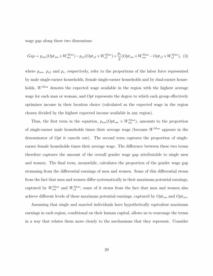
wage gap along these two dimensions:

Gap = psm(Optsm×WMaxsm )−psf (Optsf×WMax

sf )+pc2

(Optcm×WMaxcm −Optcf×WMax

cf ), (3)

where psm, psf and pc, respectively, refer to the proportions of the labor force represented

by male single-earner households, female single-earner households and by dual-earner house-

holds, WMax denotes the expected wage available in the region with the highest average

wage for each man or woman, and Opt represents the degree to which each group effectively

optimizes income in their location choice (calculated as the expected wage in the region

chosen divided by the highest expected income available in any region).

Thus, the first term in the equation, psm(Optsm × WMaxsm ), amounts to the proportion

of single-earner male households times their average wage (because WMax appears in the

denominator of Opt it cancels out). The second term captures the proportion of single-

earner female households times their average wage. The difference between these two terms

therefore captures the amount of the overall gender wage gap attributable to single men

and women. The final term, meanwhile, calculates the proportion of the gender wage gap

stemming from the differential earnings of men and women. Some of this differential stems

from the fact that men and women differ systematically in their maximum potential earnings,

captured by WMaxcm and WMax

cf ; some of it stems from the fact that men and women also

achieve different levels of these maximum potential earnings, captured by Optcm and Optcm.

Assuming that single and married individuals have hypothetically equivalent maximum

earnings in each region, conditional on their human capital, allows us to rearrange the terms

in a way that relates them more clearly to the mechanisms that they represent. Consider

20

the following algebraic rearrangement:

Gap = Optsm × (psmWMaxm − psfWMax

f ) +Optcm ×pc2

(WMaxm −WMax

f ) (4)

+(Optsm −Optsf )× psfWMaxf + (Optcm −Optcf )×

pc2WMaxf (5)

The top line of this equation (4) represents the portion of the gender wage gap that accrues

from processes that limit the earnings of women relative to men across all regions, including

blatant discrimination, penalties associated with motherhood, the sorting of women into

particular industries and occupations with lower pay, and differentials in the accumulation

of human capital. The second line (5), meanwhile, captures the portion of the gender wage

gap that stems from systematic variation in the degree to which men versus women reside

in regions where employers value their abilities and attributes.

Table 4 reports the components of this equation and the calculated amount of the gender

wage gap that could stem from gender differences in the goodness of geographic fit. The psm,

psf and pc in this table report the proportions of the blue-collar and lower-white-collar labor

force represented, respectively, by single men, by single women and by couples. We used as

the maximum wage for each individual the 90th percentile expected wage for a single man or

woman with equivalent characteristics (WMaxm and WMax

f correspond to the average of these

“maximums” for all blue-collar and lower-white-collar men and women). Using the 90th

percentile reduces the sensitivity of our decomposition to outliers.13 The Opt values report

the average percentage of this theoretical maximum achieved by each segment. Overall, our

decomposition indicates that the better matching of men relative to women to places that

value as employees their abilities and attributes might account for roughly 36% of the gender

wage gap among blue-collar and lower-level white-collar employees.

13Decomposition calculations using the 75th or 95th percentile as the maximum generated similar results.

21

Proximate versus ultimate causes

Though the evidence suggests that the undue weight that couples place on the man’s expected

earnings in choosing of where to live can account for a substantial portion of the gender wage

gap, this mechanism is but a proximate cause. It begs the question of why couples would

differ in the value that they placed on a dollar depending on who earned it. We explore

five potential possibilities: (i) structural explanations: men may have more to gain from

a particular location, (ii) intra-household bargaining: men and women care about different

dimensions in the location decision, (iii) relative resources: men use their earnings power to

dictate the location choice, (iv) a motherhood penalty: the woman allocating time to child

care or being penalized by employers, and (v) gender roles: the undervaluing of women’s

wages resulting from traditional gender roles.

Structural explanations: Our estimation strategy rules out most structural explana-

tions. For example, if men had greater variation in their earnings across regions, then one

might expect income-maximizing couples to focus on the man’s earnings in their location

decisions (Mincer 1978; Shauman and Noonan 2007). However, our empirical design esti-

mates the implicit weights attached to a unit increase in expected income for the man and

the woman. Though couples may face differences in the supplies of jobs available to each

partner, in our design, those constraints would appear in the wage equations (and hence in

the expected incomes) rather than in the implicit weights (coefficients).

One reason income-maximizing couples might not weight men’s and women’s expected

earning equivalently in our approach would be if the two differed in their income trajectories.

Gender inequality has been found to increase with age and with job tenure (Blau and Kahn

2000; Fernandez-Mateo 2009; Esteves-Sorenson and Snyder 2012); over time, men accumulate

22

more and larger raises than their female counterparts. Though economists have suggested

that women choose occupations with flatter income trajectories (Polachek 1981), these di-

verging choices and income trajectories may also reflect various forms of discrimination (Cor-

rell 2004). Regardless of the source of these differences, however, income-maximizing couples

would respond by placing greater emphasis in their decisions on the man’s job prospects since,

over time, the benefits of doing so would compound.

To examine whether differing income trajectories might account for the greater weights

given to men’s jobs, we interacted the expected incomes with industry income trajectories.

Industries vary in the rates at which employees receive raises. We essentially examine whether

couples in which the man works in an industry with a steeper wage trajectory weigh the man’s

wage more heavily. As a measure of the wage trajectory, we calculated the five-year earnings

increase for all blue-collar and lower-white-collar employees in the same two-digit industry as

the focal individual—income in 2004 divided by income in 1999. Since even within industries

men and women segregate into different jobs (Bielby and Baron 1986; England et al. 1988),

we calculated these trajectories separately for men and women.

Model 6 (Table 5) includes these interaction terms. Note that these models do not include

the “main” effects of industry wage trajectories; the conditioning in the conditional logit acts

much like a couple-specific fixed effect and therefore purges from the estimates any variables

that do not vary within couples across regions. Model 6 suggests that differences in expected

income trajectories cannot explain the greater weight given to the man’s income.

Intra-household bargaining: Another possible explanation is that men and women dif-

fer in the dimensions that attract them to particular places and therefore also over the

dimensions on which they choose to bargain in intra-household decisions. Prior research, for

example, suggests that women find it more difficult than men to separate their work and

23

social lives and that they may place greater value on living near family and friends (e.g.,

Curran and Rivero-Fuentes 2003; Mulder 2007). When choosing a place to live, they may

therefore sacrifice moving to the best place for their career to live closer to loved ones.

To assess this possibility, we constructed several variables to capture the draw of family

and friends. We began by constructing measures of distance to man’s parents and distance

to woman’s parents. We located both parents of each member of the couple in 2004 and

calculated separate logged distances in kilometers from each possible township to these lo-

cations.14 We also developed three pairs of measures to assess the importance of friends.

First, since people form strong bonds during childhood and therefore maintain preferences

for living near their hometowns (Dahl and Sorenson 2010b), we constructed measures for

the distance to man’s hometown and distance to woman’s hometown.15 Second, since people

also form friendships in other places they have lived, we created a second pair of measures:

distance to man’s prior residences and distance to woman’s prior residences. To do so, we

identified every place that each member of the couple had lived from 1980 to 2004, calcu-

lated the logged distance between each of these prior locations and every township, and then

averaged these distances. Third, we developed a measure of (probable) high school friends

(Man’s friends and Woman’s friends). Following Dahl and Sorenson (2010b), we calculated,

separately for the husband and the wife, the proportion of former classmates from the same

graduating year and secondary school living in each township, j, in 2004, and divided this

proportion by the proportion of individuals from the same school in each township that

graduated either one year before or one year after the focal individual (to control for other

factors that might influence the migration of individuals educated in one township to another

14If the parents lived at different addresses, we averaged their distances.15We do not always have information on where children lived from birth. We therefore used the location

of the person’s secondary school as a proxy for hometown.

24

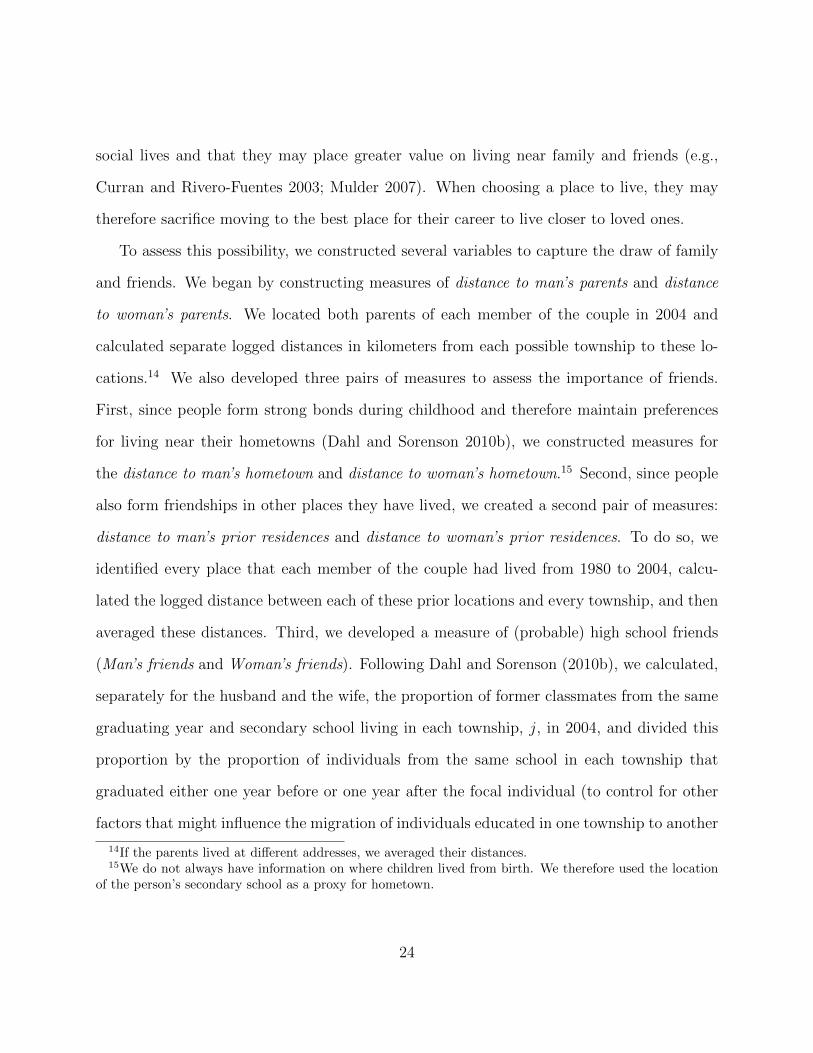
township):

friendsij =hsjτ

(hsjτ−1 + hsjτ+1)/2,

where hsjτ denotes the proportion of former students of a high school that graduated in year

τ currently employed in region j.

Couples clearly factor proximity to family and friends into their location decision (Model

7). However, couples appear to place roughly equal weighting on proximity to the husband’s

and to the wife’s family and friends; in none of the pairs of measures, can we reject the

null of equal coefficients (weights). Though these factors help to explain the locations that

couples choose, they cannot account for and appear to even partially mask asymmetry in

couples’ weightings of men’s and women’s prospective wages.

Relative resources: The relative resource hypothesis essentially argues that men can usu-

ally impose their preferences in family decisions because they control, through their income,

access to economic resources (Blood and Wolfe 1960). Though it differs from structural

explanations and the gender role hypothesis, in terms of the way in which it portrays house-

hold decision making, it also would predict that the man’s expected income would dominate

location choices (Shauman 2010).

Though difficult to distinguish in most empirical analyses, the relative weighting of prox-

imity to family and friends gives us some insight into this hypothesis. According to relative

resource theory, the husband’s bargaining power should extend also to non-economic de-

cisions (Blood and Wolfe 1960). Hence, one would expect the locations of his family and

friends to take precedence as well. Danish couples, however, appear to weight these prefer-

ences equally suggesting that the man does not simply dictate these household decisions.

25

Motherhood penalty: The tendency for mothers to leave the labor force and therefore to

accumulate less human capital has often been cited as an important contributor to the gender

wage gap (e.g. Light and Ureta 1995; Bertrand et al. 2010). Traditional gender roles place the

burden of child care on women and therefore mothers often reduce their participation in the

labor force. Even in households that share childrearing responsibilities, if employers expect

that mothers will reduce their effort at work, they may pass over them in promotions and

pay raises (e.g., Budig and England 2001). In either case, income-maximizing households

might then respond by weighting women’s wages less heavily. Consistent with this idea, prior

research has found that geographic mobility increases around the arrival of a child (Clark

and Withers 2009).

To assess the extent to which motherhood might influence couples’ location choices, we

interacted the expected incomes with an indicator variable for the presence of pre-school

children in the household (i.e. children under the age of six). Once again, these models do

not include the “main” effects since the variable does not vary within couples across regions.

Couples with pre-school children place significantly higher implicit weights on the man’s

earnings and significantly lower ones on the women’s income (Model 8).

But this factor alone cannot fully account for the asymmetry in the importance of men’s

and women’s expected earnings to the attractiveness of regions. Note that with these in-

teraction effects, the “main” effects essentially capture the relative importance of expected

incomes for couples without pre-school children. Even among this set, the coefficients indi-

cate that couples implicitly place greater emphasis on maximizing men’s incomes.

Gender roles: Finally, the greater importance of husband’s potential wage gains to loca-

tion choice may stem from within-couple beliefs about appropriate gender roles. In particular,

couples may consider the role of generating income as more of the man’s role (Hood 1983;

26

Thompson and Walker 1989; Shelton and John 1996; Potuchek 1997). If so, then they may

choose locations primarily for the benefit of the husband’s career (Bielby and Bielby 1992;

Shauman and Noonan 2007).

Connecting this possibility to the data, however, is not without difficulty. Most studies

have simply assumed that asymmetric weightings of husbands’ and wives’ human capital

reflected such gender roles. But, as noted above, the neoclassical economics model, which

assumes no such gender roles, could also account for those results. Bielby and Bielby (1992),

by contrast, made a connection between self-reported intentions to move and gender roles

through the use of survey data that included attitudinal questions. Most registry data, IDA

included, however, do not include questions on beliefs about gender roles.

Our approach stems from the idea that children learn about these norms from the in-

teractions of their parents. Psychologists have claimed that children learn gender roles by

observing their parents’ behaviors (Bandura 1977). Consistent with this idea, studies have

found that the gender roles parents display during the early years of their children’s lives have

a profound influence on the gender roles that those children assume as adults (Cunningham

2001; Fernandez et al. 2004; van Putten et al. 2008).

To assess whether the gender roles observed among parents might influence couples deci-

sions, we interacted expected wages with two indicator variables, one for the man’s parents

and a second for the woman’s. Each of these variables, man’s parent inequality and woman’s

parent inequality took a value of one if the father earned more, on average, than the mother

during the last five years, prior to age 60, in which both participated in the labor force.16 As

one would expect given the gender wage gap, fathers generally earned more than mothers.

16Continuous measures of relative income contribution by mothers produced similar, though slightlyweaker, results. Because this variable requires information on labor force participation, we excluded casesin which both parents exited the labor force before 1985.

27

But substantial variation exists. Even among this earlier generation, the woman earned more

than the man in 30% of cases.

Model 9 includes these interaction terms. Interestingly, the only significant coefficients

are the interactions between the income differential of the man’s parents with the weightings

of the man’s and the woman’s expected wages.17 Couples where the man had been exposed

to more traditional gender roles as a child – those in which his father earned more than his

mother – placed greater weights on the man’s income and lesser weights on the woman’s

earnings in their location choices. Overall, the motherhood penalty and the exposure to

more traditional gender roles can account for roughly two-thirds of the asymmetry in the

implicit weighting of men’s and women’s wages.

Discussion

Social scientists have long suspected that the location decisions of dual-earner couples might

contribute to the gender wage gap, with couples giving greater weight to men’s careers

in their choices (Mincer 1978; Bielby and Bielby 1992). Research has nonetheless been

equivocal on whether this asymmetry represents a rational response to structural constraints,

a maximization of household income, or results from enacting beliefs about traditional gender

roles. Extant research has also been largely silent on the proportion of the gender wage gap

that this allocative asymmetry might explain.

We revisited these questions using data registries maintained by Statistics Denmark.

By calculating individual-specific counterfactual wages for each region (on the basis of the

earnings of others with similar observable characteristics), we could estimate the degree to

17Though one might worry that men and women might match those with similar backgrounds (assortativemating), limiting our ability to distinguish the influence of intergenerational transmission through the man’sversus the woman’s side, gender inequality across the two sets of parents only correlated at r = .13.

28

which couples implicitly valued prospective earnings for men and for women in their location

choices. Danish couples placed much greater weight on men’s than on women’s expected

income. A decomposition of these effects determined that the resultant mismatching of

women to employers could account for up to 36% of the gender wage gap.

Our results therefore suggest that the allocation of people to places contributes impor-

tantly to gender inequality. In trying to understand the ultimate sources of these asymmetric

allocations, our analyses pointed to two prime suspects, both related to gender roles. First,

we identified a motherhood penalty. Couples with young children placed greater weight on

men’s and less weight on women’s potential earnings. This effect interestingly exists despite

the fact that Denmark has some of the most generous policies for providing state assistance

in child care (Craig and Mullan 2010). Since our estimations excluded couples in which the

mother did not maintain full-time employment, this motherhood penalty does not appear to

stem from household income maximization.

Second, we observed an undervaluation of women’s wages, particularly among couples

where the man had been exposed to more traditional gender roles as a child. Couples in

which the man’s parents – but not the woman’s – had greater gender inequality in terms

of their relative earnings had much stronger implicit weights biased toward maximizing the

man’s income. Asymmetric weighting therefore appeared primarily among couples where

the man’s parents themselves had had more traditional gender roles. It appears that gender

roles – at least in Denmark – may pass from parents to sons. Though research on the

intergenerational transmission of gender roles remains at an early stage, our results have

interesting parallels with some prior studies. Cunningham (2001), for example, reports that

the amount of time that fathers spend on housework at age one positively predicts sons

participation in household chores at age 31.

29

Though useful for empirical precision, our focus on a subset of the Danish population

raises at least two questions. First, would these joint geographic decisions also account for

a similar proportion of income inequality among professionals? On the one hand, one might

expect less asymmetry in the importance of men’s and women’s’ careers to the choices of

the highly educated. For one, those with the most traditional gender roles might not even

pursue higher education (Vella 1994). Exposure to alternative ideas through college may also

influence the college-educated to adopt more gender-egalitarian attitudes (Funk and Willits

1987). On the other hand, the consequences of locating in the right region matters much

more for these individuals. Professionals have typically developed highly specific skills and

therefore their expected earnings vary much more from one region to the next (Dahl and

Sorenson 2010a). As a consequence, even small asymmetries in the location choices of these

power couples could produce large levels of gender inequality in income. It therefore remains

an interesting open question.

Second, would one expect larger or smaller effects in other countries? Though again an

open question, we can say something about the factors that should determine the relative

importance of these geographic decisions to the gender wage gap: First, one would expect

their importance to increase with the asymmetry in the relative weightings placed by couples

on mens’ and women’s wages. On this dimension, we would expect larger differences in other

countries, as Denmark – relative to the rest of the world – has relatively low levels of gender

segregation and gender inequality (Craig and Mullan 2010; Hausmann et al. 2010). Second,

the importance of these decisions should increase with the propensity of people to move

in general. As populations become more mobile, location choices contribute more strongly

to differences across individuals in earnings. Denmark, relative to its small size, has high

levels of geographic mobility, on par with the United States (Dahl and Sorenson 2010b). By

30

contrast, many other countries have lower levels of geographic mobility and therefore these

joint choices may have less power for explaining gender inequality. Finally, the importance

of these choices should also increase with the degree of geographic variation in possible

employers. On this dimension, one would expect much larger differences in most other

countries. Denmark is relatively small and homogenous, about the size of Massachusetts,

Rhode Island and Connecticut combined. The United States as a whole, or even countries

like Italy or the United Kingdom, have much greater geographic scale and variation and

therefore much larger opportunities for location to matter.

Though additional research remains to determine the extent to which these joint decisions

influence gender inequality in other countries, our research nonetheless contributes to the

literature in multiple ways. First, we have introduced a critical test for discriminating

between the gender-neutral and gender-biased migration. Crucial to this test has been the

introduction of an approach to specifying counter-factual wages for what each member of

the couple might earn in another region. Second, we have devised a decomposition that

allows researchers to connect these joint choices to the gender wage gap and to estimate

the proportion of the gap that stems from the systematic mismatching of married women

to regions that would most highly value their abilities and attributes. Finally, our analyses

explore the ultimate mechanisms underlying these asymmetric weightings and find that – at

least among Danish blue-collar and lower-level white-collar workers – they appear to stem

from the combination of a motherhood penalty and the enactment of traditional gender roles.

Our results call additional attention to the role of allocative processes in the produc-

tion of gender inequality. They therefore bolster the literature on gender sorting, which

demonstrates that men and women pursue different kinds of careers (e.g. Tam 1997) and

find themselves employed by different organizations and in different job titles (e.g. Petersen

31

1995; Fernandez and Sosa 2005). Here, the joint decisions of couples, prioritizing the man’s

earnings in location choices, creates a matching process that results in men being systemat-

ically better fit to potential employers than their female partners.

As with other supply-side mechanisms, our results suggest that public policies for elim-

inating gender inequality face a fundamental limit if they focus only on the discriminatory

actions of employers. Even if all organizations operated in a gender-blind manner, if couples

decide to locate such that married men sort systematically into labor markets better suited

to them than their wives, then gender income inequality would still persist. That’s not to

say that public policy could not help to alleviate these disparities. But the policies to do

so would need to focus either on education, which appears to move people away from tra-

ditional gender roles, or on promoting a more diverse set of employers in all regions, which

decreases the likelihood that any individual has difficulty finding a well-matched employer

in any particular place (Sørensen and Sorenson 2007).

32

Table 1: Wage equation coefficients

Male FemaleMean SE Mean SE

Age -0.005 0.003 -0.002 0.002Experience /100 0.002 0.002 0.002 0.001Gymnasium 0.069 0.103 0.065 0.070College 0.109 0.092 0.038 0.043Firm tenure /100 -0.008 0.244 0.068 0.228Skilled blue collar 0.269 0.063 0.195 0.084Lower white collar 0.070 0.042 0.066 0.077Job change -0.017 0.042 -0.009 0.045Mover -0.110 0.059 -0.104 0.054Constant 5.525 0.160 5.122 0.136R2 0.218 0.055 0.245 0.069N 956 1,328 1,072 1,563Summary of the results of 269 regressions of 2004wage (270 for women), one per township

33

Table 2: Descriptive statistics for the choice models

Movers StayersChosen Alternate Chosen Alternate

Mean SE Mean SE Mean SE Mean SEExpected wage (male) (1000s) 244.3 52.15 242.3 50.24 224.8 43.74 232.0 46.96× wage trajectory 297.1 97.54 291.8 115.7 272.3 72.42 279.3 102.2× children 130.3 127.9 128.7 126.2 165.7 107.1 170.6 110.9× pre-school children 105.2 127.8 103.4 125.5 77.52 112.7 79.59 116.0× male’s parent inequality1 141.7 128.9 139.7 126.5 106.7 117.9 110.0 122.1× female’s parent inequality1 143.2 128.4 141.6 126.5 109.5 117.5 113.3 122.0

Expected wage (female) (1000s) 182.1 25.70 176.0 25.84 175.6 23.16 173.8 25.50× wage trajectory 230.9 49.58 225.3 69.83 224.2 45.22 222.1 65.95× children 96.83 92.87 93.81 90.08 128.8 80.46 127.5 80.27× pre-school children 77.42 92.38 74.75 89.25 59.24 84.96 58.78 84.52× male’s parent inequality1 104.8 92.62 101.0 89.40 82.41 89.57 81.53 88.92× female’s parent inequality1 106.0 92.28 102.3 89.33 85.06 89.68 84.17 89.08

Current residence 0.000 0.000 0.004 0.061 1.000 0.000 0.000 0.000Ln (Distance to home) 3.270 0.827 4.861 0.814 0.000 0.000 4.906 0.699Ln (Distance to male’s parents) 3.414 1.587 4.377 1.592 2.311 1.855 3.884 2.066Ln (Distance to female’s parents) 3.464 1.584 4.365 1.608 2.469 1.837 3.981 1.995Ln (Distance to male’s hometown) 2.870 1.766 4.391 1.637 1.508 1.882 3.741 2.185Ln (Distance to female’s hometown) 3.007 1.672 4.551 1.428 1.867 1.894 4.219 1.833Ln (Distance to male’s prior residences) 3.190 0.992 4.870 0.734 1.183 1.157 4.904 0.686Ln (Distance to females prior residences) 3.201 0.964 4.870 0.729 1.242 1.158 4.903 0.686High school friends (male) 0.657 0.746 0.065 0.297 0.655 0.686 0.055 0.277High school friends (female) 0.723 0.807 0.066 0.304 0.746 0.713 0.065 0.302N 2,995 807,005 6,952 1,870,088Due to missing data, these variables only exist for XX movers and XX stayers.

34

Table 3: Conditional logit estimates of location choice

(1) (2) (3) (4) (5)Expected wage (male) 0.003∗∗ 0.003∗∗ 0.003∗∗ 0.002∗∗

(0.000) (0.000) (0.001) (0.001)Expected wage (female) -0.004∗∗ -0.004∗∗ -0.004∗∗ -0.003∗∗

(0.001) (0.001) (0.001) (0.001)Current residence 1.644∗∗ 1.595∗∗ 1.623∗∗ 1.608∗∗ 1.960∗∗

(0.063) (0.062) (0.063) (0.063) (0.109)Ln (Distance to home) -1.817∗∗ -1.824∗∗ -1.825∗∗ -1.834∗∗ -1.611∗∗

(0.017) (0.016) (0.017) (0.017) (0.028)Labor market fixed effects (21) NO NO NO YES YESLog-likelihood -25663 -25675 -25649 -25606 -10893Observations 9,947 9,947 9,947 9,947 3,217

35

Table 4: Wage gap decomposition

Optsm (single males) 82.6%Optcm (couple males) 94.1%Optsf (single females) 83.1%Optcf (couple females) 84.1%psm (single males) 21.3%psf (single females) 23.8%pc (couples) 54.9%WMax

m (all males) 340,488WMax

f (all females) 291,217

Gap (structural) 28,017 64.1%Gap (location choice) 15,709 35.9%

Opt indicates the ratio of the expectedincome in the region of residence to themaximum expected income available inany region (WMax). p denotes theproportion of the population in each group.

36

Table 5: Conditional logit estimates on location choice

(6) (7) (8) (9)Expected wage (husband) 0.003∗∗ 0.007∗∗ 0.005∗∗ 0.003∗∗

(0.001) (0.001) (0.001) (0.001)× wage trajectory -0.000

(0.000)× pre-school children 0.005∗∗ 0.002∗

(0.001) (0.001)× husband’s parent inequality 0.005∗∗

(0.001)× wife’s parent inequality 0.001

(0.001)Expected wage (wife) -0.004∗∗ -0.006∗∗ -0.004∗∗ -0.001

(0.001) (0.001) (0.001) (0.002)× wage trajectory -0.001∗

(0.001)× pre-school children -0.007∗∗ -0.006∗∗

(0.002) (0.002)× husband’s parent inequality -0.004†

(0.002)× wife’s parent inequality -0.003

(0.002)Current residence 1.756∗∗ 2.441∗∗ 2.445∗∗ 2.317∗∗

(0.076) (0.075) (0.075) (0.084)Ln (Distance to home) -1.782∗∗ -1.023∗∗ -1.026∗∗ -1.086∗∗

(0.021) (0.027) (0.027) (0.031)Ln (Distance to husband’s parents) -0.204∗∗ -0.206∗∗ -0.201∗∗

(0.027) (0.027) (0.029)Ln (Distance to wife’s parents) -0.230∗∗ -0.231∗∗ -0.277∗∗

(0.026) (0.026) (0.028)Ln (Distance to husband’s hometown) 0.000 -0.003 -0.031

(0.023) (0.023) (0.025)Ln (Distance to wife’s hometown) -0.038† -0.042† -0.080∗∗

(0.023) (0.023) (0.025)Ln (Distance to husband’s prior residences) -0.443∗∗ -0.437∗∗ -0.376∗∗

(0.038) (0.038) (0.042)Ln (Distance to wife’s prior residences) -0.335∗∗ -0.330∗∗ -0.232∗∗

(0.038) (0.038) (0.044)Husband’s friends 0.505∗∗ 0.508∗∗ 0.561∗∗

(0.031) (0.032) (0.028)Wife’s friends 0.534∗∗ 0.534∗∗ 0.549∗∗

(0.022) (0.022) (0.025)Labor market fixed effects (21) YES YES YES YESLog-likelihood -15,960 -23,408 -23,385 -19,692Observations 8,534 9,947 9,947 7,799

37

References

Andersen, Anne Kaag. 2000. Commuting Areas in Denmark . AKF Forlaget, Copenhagen.

Bandura, Albert. 1977. Social Learning Theory . Prentice Hall, Englewood Cliffs, NJ.

Bertrand, Marianne, Claudia Goldin, Lawrence E. Katz. 2010. Dynamics of the gender gapfor young professionals in the financial and corporate sectors. American Economic Journal- Applied Economics 2(3) 228–255.

Bielby, William T., James N. Baron. 1986. Men and women at work: Sex segregation andstatistical discrimination. American Journal of Sociology 91 759–799.

Bielby, William T., Denise D. Bielby. 1992. I will follow him: Family ties, gender-rolebeliefs, and reluctance to relocate for a better job. American Journal of Sociology 97(5)1241–1267.

Blau, Francine D., Lawrence M. Kahn. 2000. Gender differences in pay. Journal of EconomicPerspectives 14(4) 75–99.

Blood, Robert O., Donald M. Wolfe. 1960. Husbands and wives: The Dynamics of marriedliving . Free Press, Glencoe, IL.

Bredgaard, Thomas, Flemming Larsen, Per Kongshøj Madsen. 2005. The flexible Danishlabour market – a review. Tech. rep., CARMA.

Budig, Michelle J., Paula England. 2001. The wage penalty for motherhood. AmericanSociological Review 66(2) 204–225.

Castilla, Emilio J. 2008. Gender, race, and meritocracy in organizational careers. AmericanJournal of Sociology 113(6) 1479–1526.

Clark, William A.V., Suzanne Davies Withers. 2009. Fertility, mobility and labour-forceparticipation: A study of synchronicity. Population, Space and Place 15(305-321).

Clark, Ximena, Timothy J. Hatton, Jeffrey G. Williamson. 2007. Explaining U.S. immigra-tion, 1971-1998. Review of Economics and Statistics 89(2) 359–373.

Cohen, Philip N., Matt L. Huffman. 2003. Individuals, jobs, and labor markets: The deval-uation of women’s work. American Sociological Review 68 443–463.

Compton, Janice, Robert A. Pollak. 2007. Why are power couples increasingly concentratedin large metropolitan areas? Journal of Labor Economics 25(3) 475–512.

38

Cooke, Thomas J. 2003. Family migration and the relative earnings of husbands and wives.Annals of the Association of American Geographers 93(2) 338–349.

Cooke, Thomas J. 2008. Migration in a family way. Population, Space and Place 14 255–265.

Correll, Shelley J. 2004. Constraints into preferences: Gender, status, and emerging careeraspirations. American Sociological Review 69(1) 93–113.

Craig, Lyn, Killian Mullan. 2010. Parenthood, gender and work-family time in the UnitedStates, Australia, Italy, France, and Denmark. Journal of Marriage and Family 72 1344–1361.

Craig, Lyn, Killian Mullan. 2011. How mothers and fathers share childcare. AmericanSociological Review 76(6) 834–861.

Cunningham, Mick. 2001. Parental influences on the gendered division of housework. Amer-ican Sociological Review 66(2) 184–203.

Curran, Sara R., Estela Rivero-Fuentes. 2003. Engendering migrant networks: The case ofMexican migration. Demography 40(2) 289–307.

Dahl, Michael S., Olav Sorenson. 2010a. The migration of technical workers. Journal ofUrban Economics 67 33–45.

Dahl, Michael S., Olav Sorenson. 2010b. The social attachment to place. Social Forces 89633–658.

Duncan, R. Paul, Carolyn Cummings Perrucci. 1976. Dual occupation families and migra-tion. American Sociological Review 41(2) 242–261.

England, Paula, George Farkas, Barbara Stanek-Kilbourne, Thomas Dou. 1988. Explain-ing occupational sex segregation and wages: Findings from a model with fixed effects.American Sociological Review 53(4) 544–558.

Esteves-Sorenson, Constanca, Jason Snyder. 2012. The gender earnings gap for physiciansand its increase over time. Economic Letters 116 37–41.

Fernandez, Raquel, Alessandra Fogil, Claudia Olivetti. 2004. Mothers and sons: Preferenceformation and female labor force dynamics. Quarterly Journal of Economics 119(4) 1249–1299.

Fernandez, Roberto M., Lourdes Sosa. 2005. Gendering the job: Networks and recruitmentat a call center. American Journal of Sociology 111 859–904.

39

Fernandez-Mateo, Isabel. 2009. Cumulative gender disadvantage in contract employment.American Journal of Sociology 114(4) 871–923.

Funk, Richard B., Fern K. Willits. 1987. College attendance and attitude change: A panelstudy, 1970-81. Sociology of Education 60 224–231.

Groshen, Erica L. 1991. The structure of the female/male wage differential: Is it who youare, what you do, or where you work? Journal of Human Resources 26(3) 457–472.

Gupta, Nabanita Datta, Donna S. Rothstein. 2005. The impact of worker and establishment-level characteristics on male-female wage differentials: Evidence from Danish matchedemployee-employer data. Labour 19(1) 1–34.

Hausmann, Ricardo, Laura D. Tyson, Saadia Zahidi. 2010. The Global Gender Gap Report .World Economic Forum, Geneva.

Hood, Jane C. 1983. Becoming a Two-Job Family . Praeger, New York.

Hook, Jennifer L. 2010. Gender inequality in the welfare state: Sex segregation in housework,1965-2003. American Journal of Sociology 115(5) 1480–1523.

Jacobsen, Joyce P., Laurence M. Levin. 1997. Marriage and migration: Comparing gainsand losses from migration for couples and singles. Social Science Quarterly 78(3) 688–709.

Kilbourne, Barbara Stanek, George Farkas, Kurt Beron, Dorothea Weir, Paula England.1994. Returns to skill, compensating differentials, and gender bias: Effects of occupationalcharacteristics on the wages of white women and men. American Journal of Sociology100(3) 689–719.

Korpi, Martin, William A.V. Clark, Bo Malmberg. 2011. The urban hierarchy and domesticmigration: The interaction of internal migration, disposable income and the cost of living,sweden 1993-2002. Journal of Economic Geography 11 1051–1077.

LeClere, Felicia B., Diane K. McLaughlin. 1997. Family migration and changes in women’searnings: A decomposition analysis. Population Research and Policy Review 16 315–335.

Light, Audrey, Manuelita Ureta. 1995. Early-career work experience and gender wage dif-ferentials. Journal of Labor Economics 13(1) 121–154.

Long, Larry H. 1974. Women’s labor force participation and the residential mobility offamilies. Social Forces 52 342–348.

Massey, Douglas S., Kristin E. Espinosa. 1997. What’s driving Mexico-U.S. migration? Atheoretical, empirical, and policy analysis. American Journal of Sociology 102(4) 939–999.

40

McFadden, Daniel. 1974. Conditional logit analysis of qualitative choice behavior. P. Zarem-bka, ed., Frontiers of Econometrics . Academic Press, New York, 105–142.

McKinnish, Terra. 2008. Spousal mobility and earnings. Demography 45(4) 829–849.

Mincer, Jacob. 1978. Family migration decisions. Journal of Political Economy 86(5) 749–773.

Mulder, Clara H. 2007. The family context and residential choice: A challenge for newresearch. Population, Space and Place 13 265–278.

Offer, Shira, Barbara Schneider. 2011. The gender gap in time-use patterns: Parents’ mul-titasking and well-being. American Sociological Review 76(6) 809–833.

Petersen, Trond. 1995. Separate and unequal: Occupation-establishment sex seggregationand the gender wage gap. American Journal of Sociology 101(2) 329–365.

Polachek, Solomon. 1981. Occupational self selection: A human capital approach to sexdifferences in occupational structure. Review of Economics and Statistics 58 60–69.

Potuchek, Jean L. 1997. Who Supports the Family? Gender and Breadwinning in Dual-Earner Marriages . Stanford University Press, Stanford, CA.

Presser, Harriet B. 1996. Employment schedules among dual-earner spouses and the divisionof household labor by gender. American Sociological Review 59(3) 348–364.

Quillian, Lincoln. 1999. Migration patterns and the growth of high-poverty neighborhoods,1970-1990. American Journal of Sociology 105(1) 1–37.

Sandell, Steven H. 1977. Women and the economics of family migration. Review of Economicsand Statistics 59 406–414.

Shauman, Kimberlee A. 2010. Gender asymmetry in family migration: Occupational in-equality or interspousal comparative advantage? Journal of Marriage and Family 72375–392.

Shauman, Kimberlee A., Mary C. Noonan. 2007. Family migration and labor force outcomes:Sex differences in occupational context. Social Forces 85(4) 1735–1764.

Shelton, Beth Anne, Daphne John. 1996. The division of household labor. Annual Reviewof Sociology 22 299–322.

Soons, Judith P.M., Matthijs Kalmijn. 2009. Is marriage more than cohabitation? well-beingdifferences in 30 european countries. Journal of Marriage and Family 71(5) 1141–1157.

41

Sørensen, Aage B. 1996. The structural basis of social inequality. American Journal ofSociology 101 1333–1365.

Sørensen, Jesper B., Olav Sorenson. 2007. Corporate demography and income inequality.American Sociological Review 72(5) 766–783.

Tam, Tony. 1997. Sex segregation and occupational gender inequality in the United States:Devaluation or specialized training? American Journal of Sociology 102(6) 1652–1692.

Tenn, Steven. 2010. The relative importance of the husband’s and wife’s characteristics infamily migration, 1960-2000. Journal of Population Economics 23 1319–1337.

Thompson, Linda, Alexis J. Walker. 1989. Gender in families: Women and men in marriage,work, and parenthood. Journal of Marriage and Family 51(4) 845–871.

Train, Kenneth. 2003. Discrete Choice Methods with Simulation. Cambridge UniversityPress.

U.S. Department of Labor. 2001. Highlights of women’s earnings in 2000. Tech. rep., Bureauof Labor Statistics Report 952.

van Putten, Anne E., Pearl A. Dykstra, Joop J. Schippers. 2008. Just like mom? theintergenerational reproduction of women’s paid work. European Sociological Review 24(4)435–449.

Vella, Francis. 1994. Gender roles and human capital investment: The relationship betweentraditional attitudes and female labour market performance. Economica 61(242) 191–211.

42