geomechanical study of bowland shale...
TRANSCRIPT

Geomechanical Study of Bowland Shale Seismicity
Synthesis Report
Prepared by
Dr. C.J. de Pater and Dr. S. Baisch
2 November 2011

Geomechanical Study of Bowland Shale Seismicity
Synthesis Report
2 November 2011
This report was commissioned by Cuadrilla Resources Ltd in June 2011 to study the relationship between Cuadrilla’s operations and two small earthquakes that occurred near the Preese Hall wellsite in Lancashire, UK. This synthesis report utilizes independent technical reports prepared by Seismik (lead investigator Dr. Leo Eisner), Q-con (lead investigator Dr. Stefan Baisch), Geosphere (Dr. Tim Harper), StrataGen (lead investigator Dr. C.J. de Pater) and Baker-GMI (lead investigator R. Guises). Well data and technical information was provided by Cuadrilla Resources.
DISCLAIMER
Neither StrataGen Delft BV nor Q-con GmbH nor any person acting on behalf of StrataGen
or Q-con:
• Makes any warranty or representation, express or implied, with respect
to the accuracy, completeness, or usefulness of the information contained in this
report, or that the use of any apparatus, method, or process disclosed in this
report may not infringe privately owned rights; or
• Assumes any liability with respect to the use of, or for damages resulting from
the use of, any information, apparatus, method, or process disclosed in this
report.

iii
Summary Over the past decades, experience gained from mapping hundreds of hydraulic fracture treatments with downhole geophones has shown that seismic events induced by these fracture treatments normally have a magnitude much lower than 0 on the Richter scale. That is the reason for using downhole receivers, since these events are hard to detect at the surface. Stronger events occur when some of the fluid penetrates into faults and in rare cases, events with magnitude up to 0.8 ML have been detected. Another observation is that injection volume has an influence on micro-seismic magnitude: larger injected fluid volumes tend to yield stronger events. However, even mapping of many treatments in US shale plays has only shown events up to 0.8 ML for a treatment volume of 15,000 bbls (N.R. Warpinski, private communication). There are only two documented cases of a hydro-frac treatment causing events up to magnitude 1.9 ML and 2.8 MD, respectively (from massive hydro-frac treatments in Oklahoma; Luza and Lawson, 1990; Holland, 2011). The seismic events observed after two treatments in the Preese Hall well are therefore quite exceptional. Two events reported by BGS (magnitudes 2.3 and 1.5) and 48 much weaker events have been detected, and it is therefore hard to dismiss them as an isolated incident. The observed events are already 2 orders of magnitude stronger than normally observed from hydraulic fracturing induced seismicity and if future stimulation treatments again induce seismicity, it is imperative that the maximum magnitude can be estimated. It only appears feasible to establish an upper bound on the seismic magnitude if the estimation of that bound can be based on a clear understanding of the mechanism behind the past events. In this report, the probable mechanism of the events is described based on a careful technical analysis of all available data. It will be shown that many factors coincided to induce these seismic events, which are unusual for stimulation treatments. Since the chance for any single factor to occur is small, the combined probability of a repeat occurrence of a fracture induced seismic event with similar magnitude is quite low.
Input data The most important data to constrain the geomechanical model are the seismic events themselves. There are three pieces of information that are essential:
• The temporal behavior: the strongest events occurred late in the sequence and in most cases seismicity started some time after injection started
• The signature of the seismic events: since the wave forms are all similar, the source of the events must be a single slip plane or perhaps a series of closely spaced slip planes that cannot be resolved because of the wave length of the signals and the detection distance.
• Locations of the largest seismic events appear to be in the close vicinity of the injection well. The earth model that is used to interpret the events and their relation to the injections consists of the stress components, the lithology and the rock properties as a function of depth. Log and core data are available to calibrate this earth model and additionally the injection pressure can be used to infer the minimum stress. After the second treatment, which induced the strongest seismic event, it was noticed that the 5½ in production casing was ovalized over a considerable distance of hundreds of ft. This ovalization is possibly related to the fault slip, but in view of the large interval of deformation it is most likely that the wellbore deformation is caused by shear slip on bedding planes, which is possibly associated with the fault slip. Finally, the pressure recorded during the fracture treatments yields information about the fracture system which has been opened by the injections. The flow-back of water after the fracture treatments also yields information on the fracture system and its connectivity.
Seismic data interpretation A catalogue of all seismic activity has been compiled consisting of 50 events. The timing of the events shows that the process driving the events has a time scale of many hours. So, it is unlikely that the actual opening of the hydraulic fractures induced the events, since the elastic response would be immediate. Fluid pressure on the fault, however, has a natural time scale, depending on fault transmissibility and storage, which does fit the observed time delay.

iv
Since all seismic signals show the same character, their focal mechanism and travel paths must be very similar and resolving the focal mechanism of one event is sufficient to characterize them all. Due to the small number of only two (local) recording stations, hypocenter locations and focal mechanisms are not well constrained by observation data (Figures 11 and 18 in Seismik, 2011). Observations are, however, consistent with strike-slip slippage on a sub-vertical plane.
Geomechanical model and event simulation The geomechanical model confirms that the Bowland Shale consists of impermeable, hard rock and that the stress regime is strike-slip. This stress regime implies a large difference between the horizontal stresses. The stress difference obtained from minifrac pressure declines and image log break-outs is some 4000 psi. This is one of the special circumstances that favours the occurrence of seismicity, since the stress difference in US shale plays is normally less than a few hundred psi. The stress regime (strike/slip) is compatible with the indicated focal mechanism. The plane is constrained by the seismic observations, but the fluid injection into the fault has not been measured. A likely candidate for the fault plane has been identified near the bottom of the well in the image log. That implies that the wellbore deformation higher up in the well was not caused by the fault slip. Since bedding planes which had undergone shear have been found in the core, it is possible that opening of bedding planes at high injection pressure resulted in shearing that caused the wellbore deformation. Perhaps the bedding planes played a role in the path for the fluid, but it is also possible that the fracture system connected the perforated intervals in stage 2 to the fault. Since the seismic events are driven by fluid pressure on the fault, the simulation of seismicity is performed with a fault model, assuming that a large part of the injected water penetrates the fault. The occurrence of the larger magnitude events a long time after the injection can be readily explained by this model. The fluid pressure decays slowly after the injection and the pressure disturbance spreads out over the fault area. Although the pressure level becomes smaller with time and distance, there is still sufficient pressure to cause fault slip. For a critically stressed fault, fault slip can be caused by much smaller overpressures than those applied during the treatment. Since the fault model is based on elastic interaction between fault patches, the model can simulate slippages on a single patch and its interaction with neighbouring patches. If many adjacent slippages combine, this results in a greater magnitude tremor. The model simulation results compare favourably with the observed pattern, using reasonable assumptions for the fault properties (transmissibility and storage). The potential for upward fluid migration can be assessed from the interpreted fracture height and size of the fault. It is concluded that the fracture system and fault are fully contained in the Bowland shale and the impervious overburden above it, so that fluid is contained.
Seismic magnitude and hazard Based on the physical model, which is calibrated on the observed seismicity, the maximum magnitude which can be expected for future treatments can be estimated; that is to say, treatments that would be repeated under almost the same geologic conditions as encountered in the Preese Hall well. For instance, it is unlikely that another well will encounter a similar fault with the same critical stresses and high transmissibility into which fluid can be pumped. However, even with such an unlikely scenario the maximum magnitude is likely to not exceed ML=3, based on the modeling of the seismicity. Based on the ground motion observed in the Preese Hall seismic events, the ground motion which could be expected for future events can be accurately predicted. This analysis provides the basis for a traffic light system that can be used for mitigating the chance of an earthquake exceeding the safe limit.
Objectives and Conclusions Establish mechanism of seismicity
• Most likely, the repeated seismicity was induced by direct injection of fluid into the same fault zone. Slippage of the fault induced by high pressure occurred with the strongest events after the injection, since the pressure spread out over a larger area causing the largest event 10 hours after the injection in stage 2.
Estimate of maximum magnitude of seismic events induced by future fluid injection • Based on the seismic observations a simplified model was calibrated that predicts a maximum event
magnitude of ML=3 as a worst case.

v
Evaluation of potential for upward fluid migration. • In the worst case, the fluid could migrate upwards along a potential fault plane by 2000 ft. Because
of the presence of a very thick impermeable formation overlying the Bowland shale and the Permian anhydrites that will act as barrier, there is negligible risk of fluid breaching into permeable layers.
Evaluate seismic hazard related to fault slippage in the target formation: what damage to surface structures could be done by a given event.
• Even the maximum seismic event is not expected to present a risk. In the UK area near Lancashire there have been many seismic events induced by mining induced seismicity that caused events up to magnitude ML=3.1 (Kusznir Bishop et al.,1980; Bishop et al., 1994; Lovell Bishop et al.,1997; Redmayne, 1988). Some of these events caused slight damage, but the seismic events originated from a depth of 1 km. At a depth of 3 km, these events may not have caused any damage.
• Based on the internationally accepted German standard for ground vibrations, a very conservative maximum seismic magnitude of ML=2.6 is adopted as the allowable limit to the seismicity. This ensures that no damage at all could be done to surface structures near a well that is fracture stimulated.
Mitigate the magnitude of seismic events. • From the observations and modeling we can identify two potential mitigation measures: rapid fluid
flow back after the treatments and reducing the treatment volume. Furthermore, intervals close to a fault (as identified with image logs) should be avoided.
• Mitigation of seismicity can be achieved by monitoring seismicity during the treatments and taking appropriate action when seismic magnitude exceeds the limit set by the so-called traffic light system:
o Magnitude smaller than ML=0: regular operation o Magnitude between ML=0 and ML=1.7: continue monitoring after the treatment for at least 2
days until the seismicity rate falls below one event per day. o Magnitude > ML=1.7: stop pumping and bleed off the well, while continuing monitoring.
• An important result from the identified mechanism is that measurable seismicity is unlikely to occur in the next wells. The induced seismicity depends on three factors: presence of a critically stressed fault, a fault that is transmissible so that it accepts large quantities of fluid and a fault that is brittle enough to fail seismically. One of the reasons seismicity in propped fracture treatments is weak is that most fluid is pumped with significant sand concentration. Therefore it is likely that the slurry cannot easily enter a fault which will have a much smaller aperture than a hydraulic fracture. The seismic events imply that in the Preese Hall well a large fraction of the fluid entered a fault and this is one of the key factors that are unlikely to occur again in the other wells in the Bowland Shale.
• It is possible that the seismicity originated in the basement and that the hard limestone strata played a role in the seismicity. Future monitoring of treatments should resolve the depth location, which could help mitigating seismicity by avoiding injection into strata that are prone to strong induced seismicity.

vi
Contents SUMMARY .................................................................................................................................................... III
Contents ..................................................................................................................................... vi
List of Figures .......................................................................................................................... vii
List of Tables ............................................................................................................................. ix
Glossary ....................................................................................................................................... x
Nomenclature ........................................................................................................................... xii 1 INTRODUCTION ........................................................................................................................................ 1
2 DATA BASE ................................................................................................................................................. 2
Geology ....................................................................................................................................... 2
Log, core and injection data ...................................................................................................... 10
Geomechanical Earth Model ..................................................................................................... 10
Rock properties ......................................................................................................................... 10
Global Stress Model .................................................................................................................. 18
Treatments ................................................................................................................................. 21
Seismic data ............................................................................................................................... 23
Wellbore deformation................................................................................................................ 27 3 MECHANISM OF WELLBORE DEFORMATION ............................................................................ 30
4 CASING DEFORMATION AND WELLBORE INTEGRITY ........................................................... 33
5 MECHANISM OF SEISMICITY ............................................................................................................ 36
6 MAXIMUM MAGNITUDE OF FUTURE SEISMIC EVENTS .......................................................... 37
7 POTENTIAL FOR UPWARD FLUID MIGRATION .......................................................................... 39
8 SEISMIC HAZARD RELATED TO SEISMICITY .............................................................................. 42
9 MITIGATION OF THE MAGNITUDE OF SEISMIC EVENTS ....................................................... 45
10 FUTURE STIMULATION TREATMENTS ........................................................................................ 48
11 DISCUSSION AND CONCLUSIONS ................................................................................................... 49
Conclusions ............................................................................................................................... 51
References ................................................................................................................................. 53

vii
List of Figures Figure 1: Regional setting of the Bowland basin (based on Fraser and Gawthorpe 1990). ............... 2
Figure 2: Evolution of Dinantian-Namurian deltaic-turbidite systems in northern England (after Fraser and Gawthorpe 2003). ...................................................................................................................... 3
Figure 3: Stratigraphical summary of the Preese Hall-1 well ............................................................. 4
Figure 4: Biostratigraphical zonation and correlation of Preese Hall-1 and Thistleton-1. ................. 5
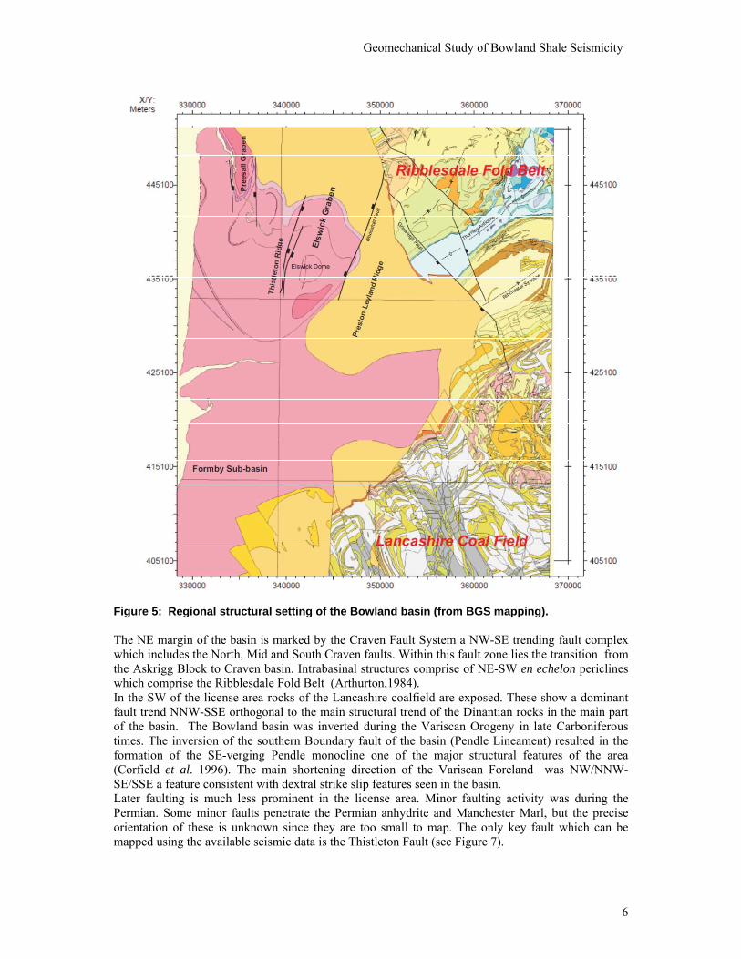
Figure 5: Regional structural setting of the Bowland basin (from BGS mapping). .......................... 6
Figure 6: Top Carboniferous (depth in ft) with the location of the PH-1 well and the seismic line (blue) in Figure 8 which is offset from the well. ...................................................................................... 7
Figure 7: Reprocessed seismic section showing the location of the Thistleton Fault and key horizons in the proximity of Preese Hall-1 and Thistleton-1. ............................................................................. 7
Figure 8: Reprocessed seismic section showing the two fault types, A and B in the proximity of Preese Hall-1 and Thistleton-1. The seismicity was caused by a type A fault that is contained in the Carboniferous. ................................................................................................................................................... 8
Figure 9: Perspective view of the Woodsfold Fault system looking NE. The map is a TWT coloured by dip where blue=0 and black=50. ...................................................................................................... 8
Figure 10: Burial history model of strata penetrated by the Preese Hall-1 well. ................................ 9
Figure 11: Preese Hall-1 completion diagram. From Cuadrilla Resources Ltd. ................................. 11
Figure 12: Left plot: Log-derived Young’s modulus (GPa) recorded by Weatherford, with the gamma ray curve (API); the log was slightly filtered for clarity. Right plot: Poissons ratio from slow wave travel time plotted from the Weatherford cross dipole log for the interval 7500-9250 ftMD. (Poisson’s ratios derived from the fast waves, not shown here are typically slightly lower.) ............................... 12
Figure 13: Slickensided and polished bedding surface in core recovered from well PH-1. Left: 8185 ftMD). Right: 6835.5 ftMD. ................................................................................................................... 13
Figure 14: Mudstone sample for sliding friction tests (Sample 13; Box 13, 6813.2-6816.5 ftMD)) . 14
Figure 15: Carbonate siltstone for sliding friction tests (Sample 18; Box 18, 6830.0-6833.1 ftMD) 14
Figure 16: Results of mudstone and dark band sliding friction experiments and one failure of intact mudstone. From Rutter (2011b). ................................................................................................ 15
Figure 17: Results of carbonate siltsone friction experiments. From Rutter (2011b). ...................... 16
Figure 18: Log based rock strength (UCS) calculation from well Preese Hall 1 (depth interval from 1,800 ft. to 9,100 ft. MDKB). The left hand side log shows the gamma ray response, used to identify the lithology (yellow- sandstones, brown-shales, white-anhydrite and blue–limestones). The rock strength is then calculated using the sonic (compressional) log and the appropriate relationship for all the lithologies. The neutron porosity log was utilized to estimate the rock strength of the carbonate rocks. Poisson’s ratio and internal friction were also calculated from log derived relationships based on acoustic velocities. The red points on the UCS track are the calibration points (from uniaxial and triaxial tests) obtained from laboratory tests (taken from: GMI, 2011). .................................... 18
Figure 19: Example of stress-induced wellbore failure-breakouts (in purple rectangles) and Drilling Induced Tensile Fractures (blue lines) from electrical image data in well Preese Hall 1 (here we also show the corresponding quality of the data as wells as caliper log that provides further evidence of the enlargement of the wellbore- third track from right) (taken from: GMI, 2011). ....................... 19
Figure 20: Minimum stress, σh,min, maximum stress, σH,max, vertical stress, σV, and pore pressure, p, inferred from density logs, minifracs, FIT tests and image log interpretation with the help of laboratory strengths tests on core samples (adapted from: GMI, 2011). ..................................................... 20

viii
Figure 21: Treatment data of stage 1 in well PH1. Bottom Hole pressure and injection rate (upper diagram) and Well Head pressure and proppant concentration (lower diagram). ..................................... 21
Figure 22: Treatment data of stage 2 in well PH1. Bottom Hole pressure and injection rate (upper diagram) and Well Head pressure and proppant concentration (lower diagram). ..................................... 22
Figure 23: Availability of seismic stations over the treatment period vs date (in MM/DD/YYYY format). Local stations were installed after the first seismic event was reported by BGS (Seismik, 2011). 23
Figure 24: Overview of injection volume and seismicity of all treatment stages in well PH1. More small events were recorded in May because the monitoring system was improved with local stations. 23
Figure 25: PH1 Stage 2 data of well PH1: injected volume with seismic events (lower diagram) and pressure and rate (upper diagram). The strongest event occurred 10 hours after shut-in. BHP was corrected for perforation and near-wellbore friction. ...................................................................................... 24
Figure 26: PH1 stages 4 and 5: injected and flowback volume with seismic events (lower diagram) and pressure and rate (upper diagram). The strong events after stage 4 occurred while the well was shut in with high pressure. ..................................................................................................................... 25
Figure 27: Zoom in on stage 4 in well PH1: injected and flowback volume with seismic events (lower diagram) and pressure and rate (upper diagram). The strong event after stage 4 occurred again about 10 hours after shut-in, as in stage 2. ................................................................................................ 26
Figure 28: Traces of seismic events vs time, observed on the local station HHF, normalized on maximum amplitude. The two upper diagrams show the horizontal components, which picked up the shear waves and the lower diagram shows the vertical component with the compressional wave. The records are remarkably similar in shape, showing that all events originated from the same source plane. . 26
Figure 29: Minimum and maximum casing radius as measured over the deformed interval. The two passes (1,2) repeated fairly well. ........................................................................................................... 27
Figure 30: Variation of maximum and minimum casing radii derived from the 24arm caliper log from 8350‐ 8665ftMD in Well PH‐1. Three of the casing collar locations are also shown.There was some deviation over a very large interval, but more than 0.5 in ovalization occurs from 8500-8740 ftMD. ..... 28
Figure 31: Azimuth of the least casing diameter for the interval 8400‐8670 ftMD in Well PH‐1 (pink dots). Since the fingers are spaced by 15o the azimuth shows digital noise by 15o. Bedding strike, interpreted from the image log, is plotted as a continuous blue line. Note that the azimuth is plotted only for a 0‐1800 range. ............................................................................................................................. 28
Figure 32: Casing deformation overlain by Gamma ray (grey; x0.1). 3 casing collars are located. .. 30
Figure 33: Minimum radius of the ovalised casing for the interval 8200‐8725ftMD and bedding dip (deg./10). .................................................................................................................................... 32
Figure 34: Casing Deformation in Preese Hall (vertically scaled drawing) ....................................... 33
Figure 35: Casing Deformation in Context With Overall Wellbore Integrity (vertically scaled drawing for deformed interval plus perforated intervals) .............................................................................. 34
Figure 36: Maximum earthquake magnitude simulated in different numerical models assuming a different storage coefficient in the plane of weakness. Different symbols indicate to what extend simulation results match observation data. The best fitting model is indicated by a red square. Models consistent with observed hydraulic pressures and timing of the maximum magnitude event during shut-in are marked by red crosses. Note that data points of different models may plot at the same location. See text for details.. ................................................................................................................................. 37
Figure 37: Confinement of injected fluid inside the Injection Layer should be evaluated with respect to the Containment Layer (Millstone grit formation) and the overlying Confinement Layer. ............ 39

ix
Figure 38: Stimulated zone after the end of the numerical simulation in plane view. Colors denote transmissibility values in the fault zone according to the color map. The highly stimulated area (white) extends laterally over a radius of approximately 1400 ft (425 m). ............................................ 40
Figure 39 : Guideline values for peak particle velocity (mm/s) measured at the foundation of the building according to German DIN4150-3. Line 1 refers to buildings used for commercial purposes, industrial buildings and buildings of similar design. Line 2 refers to dwellings and buildings of similar design and/or use. Line 3 refers to structures that, because of their sensitivity to vibration, do not correspond to those listed in lines 1 and 2 and are of great intrinsic value (e.g. buildings that are under a preservation order). ......................................................................................................................................... 42
Figure 40: Guidance values for peak particle velocity (mm/s) measured at the base of the building according to BS 7385, part 2. Line 1 refers to reinforced or framed structures, industrial and heavy commercial buildings. Line 2 refers to unreinforced or light framed structures, residential or light commercial type buildings. .................................................................................................................................... 43
Figure 41: Peak ground velocity (PGV) as a function of distance for different signal frequencies according to the legend. PGV has been determined for an ML=2.6 earthquake at 3 km depth. Frequency dependent PGV threshold values according to DIN4150, line 2 (compare Figure 39) are indicated by dotted lines using the same color encoding. Note that the DIN4150 threshold value is reached by the 50 Hz curve (red line). .................................................................................................................................... 43
Figure 42: Injection volumes, flowback volumes and well head pressure after the flowback period for each treatment stage in well PH1. ...................................................................................................... 45
Figure 43: Traffic light system proposed for future treatments in the Bowland Shale. ..................... 46
Figure 44: PH1 wellbore diagrams during the frac stages. ................................................................. 56
Figure 45: PH1 wellbore diagrams during the flow back periods. For the production test, a tubing was run. ................................................................................................................................................... 56
List of Tables Table 1: Sequence investigated in terms of geomechanical state. ...................................................... 10
Table 2: Treatment data of the minifrac and main fracture stages. .................................................... 22
Table 3: Overview of treatment dates, shooting of perforations, installing or milling of plugs and flowback periods. ....................................................................................................................................... 57

x
Glossary
Terminology Definition
butterfly effect
The butterfly effect is the sensitive dependence on initial conditions, where a small change at one place in a nonlinear system can result in large differences to a later state.
Throughout this document, the terminology butterfly effect is used to characterize non-linear behavior, where small, localized stress perturbations on a fault lead to a large magnitude earthquake.
conservative risk appraisal Parameters on which the risk appraisal is based on are chosen such that the resulting seismic risk tends to be overestimated.
earthquake magnitude
Quantifies the energy contained in an earthquake. Different magnitude scales exist. Throughout this document, earthquake magnitude refers to the local magnitude ML also known as Richter magnitude.
induced seismicity Seismic activity caused by subsurface operations. In the context of fluid-injection induced seismicity, radiated seismic energy is provided by the release of tectonic energy.
post-injection seismicity
Earthquake activity occurring after a hydraulic treatment has been terminated. The driving force for post-injection seismicity is (temporarily) ongoing pressure diffusion at the reservoir boundaries.
seismic hazard Quantifies the probability of occurrence of an earthquake of a certain magnitude in a certain region.
seismic intensity
Qualitative classification of the size of an earthquake on a scale from 1 to 12. The scale quantifies the effects of an earthquake on the Earth's surface, humans, objects of nature, and man-made structures. The EMS-98-scale is the most commonly used scale (European Macroseismic Scale 1998).
seismic moment A measure for the strength of an earthquake. Seismic moment can be converted to magnitude using empirical relations.
seismic risk Quantifies the probability of occurrence of economic damage for a specified location and time period.
critically stressed On a critically stressed fault, small stress perturbations (in the order of a few MPa or less) may induce earthquakes.
stress drop The (static) stress drop defines the mean stress difference between the stress-state prior to an earthquake and the stress-state after the earthquake has occurred.

xi
Terminology Definition
vulnerability Quantifies the damage associated with an earthquake of a certain intensity.
proppant Sand or ceramic particles added to the injection fluid, that keep the fracture open after relieving the pressure
Friction coefficient Ratio between shear stress and normal stress for which sliding occurs on a plane
Effective stress Stress that controls rock behavior, for failure it is total stress minus pore pressure, for deformation it is total stress minus Biot coefficient times pore pressure
Stress gradient Stress divided by depth, mostly related to minimum stress
Stress orientation Stress direction in the horizontal plane, mostly related to maximum stress
Propagation gradient Pressure at the entrance of the fracture system during injection, divided by depth
ISIP Instantaneous shut-in pressure
SQRT plot Pressure decline plotted vs square root of shut-in time
G-function Fluid loss function that forms the basis of a time transform for plotting the pressure decline taking into account the leak-off history
Perforation friction Friction pressure drop over the perforations
Near-wellbore friction Friction pressure drop over the part of the fracture system close to the wellbore, this pressure drop disappears within minutes after shut-in
Transmissibility Measure for the conductivity for fluid flow through reservoirs (permeability times height) or faults (permeability times aperture)
Storage capacity Specific volumetric compliance (per unit area); compressibility times porosity times width for fault zone and compressibility times porosity times height for reservoir

xii
Nomenclature Units: SI (m= metre, s= second, Pa=Pascal); Dimensions: m=mass, L=length, t=time Variable Description Field Units SI Units Dimensions
E : Young's modulus [106 psi] [Pa] (m/Lt2) G : Young's modulus [106 psi] [Pa] (m/Lt2) k : permeability [mD] [m2] (L2) Lf : fracture length [ft] [m] (L) p : pressure [psi] [Pa] (m/Lt2) pc,G : closure pressure from G-plot [psi] [Pa] (m/Lt2) pc,sqrt : closure pressure from √time plot [psi] [Pa] (m/Lt2) pfl : fluid pressure [psi] [Pa] (m/Lt2) Qi : injection rate [bbl/min] [m3/s] (L3) T : tensile strength [psi] [Pa] (m/Lt2) wf : fracture width [in] [m] (L) Xf : fracture half length [ft] [m] (L) φ : porosity [-] [-] (-) η : viscosity [cP] [Pa s] (m/Lt) μ : friction coefficient [-] [-] (-) ρ : fluid density [ppg] [kg/m3] (m/L3) σH,max : maximum horizontal stress [psi] [Pa] (m/Lt2) σh,min : minimum horizontal stress [psi] [Pa] (m/Lt2) σn : normal stress [psi] [Pa] (m/Lt2) σV : vertical stress [psi] [Pa] (m/Lt2) τ : shear stress [psi] [Pa] (m/Lt2) Conversion Factors: 1 inch = 0.0254 m = 25.4 mm 1 ft = 0.3048 m 1 cP = 0.001 Pa s 1 lbf s ft -2 = 47.88 Pa s 1 gallon = 3.7853 l 1 barrel = 158.987 l =0.158987 m3 1 bbl/min = 0.00265 m 3 s -1 1 mD = 9.9E-16 m2 1 m = 39.3701 inch = 3.2808 ft 1 Pa s = 1000 cP = 0.0209 lbf s ft -2 1 kg = 2.2046 lb 1 l = 0.2642 gallon 1 m3 = 6.2898 bbl 1 m3 s-1 = 377.39 bbl/min BCF: Billion cubic feet BHP: Bottom Hole pressure, corrected for perforation and near-wellbore friction EMW: Equivalent Mud weight

xiii
FIT: Formation Integrity Test MD: Measured depth OGIP: Original Gas In Place TVDSS: True vertical depth sub-sea UCS: Unconfined Compressional Strength WHP: Well head pressure


1 Introduction
1
1 Introduction Over the past decades, experience gained from mapping thousands of fracture treatments with downhole geophones has shown that seismic events caused by these fracture treatments normally have a magnitude much lower than 0 on the Richter scale. That is the reason for using downhole receivers, since these events are hard to detect at the surface. Stronger events occur when some of the fluid penetrates into faults and in rare cases, events with magnitude up to 0.8 ML have been detected. Another observation is that injection volume has an influence on micro-seismic magnitude: larger injections tend to yield stronger events. However, even mapping of many treatments in US shale plays has only shown events up to 0.8 ML for a treatment volume of 15,000 bbls. There are only two documented cases of a hydro-frac treatment causing stronger events up to magnitude 1.9 and 2.8 MD, respectively (from massive hydro-frac treatments in South-Central Oklahoma; Luza and Lawson, 1990; Holland, 2011). The seismic events observed after two treatments in the Preese Hall well are therefore quite exceptional. Two events were reported by BGS (with magnitude 2.3 and 1.5) and 48 much weaker events have been detected, and it is therefore hard to dismiss them as an isolated incident. The observed events are already 2 orders of magnitude stronger than normally observed from hydraulic fracturing induced seismicity and if future stimulation treatments again induce seismicity, it is imperative that the maximum magnitude can be estimated. It only appears feasible to establish an upper bound on the seismic magnitude if the estimation of that bound can be based on a clear understanding of the mechanism behind the past events. Seismicity associated with stimulation treatments in the Preese Hall 1 well exhibits similar characteristics compared to seismicity induced by hydraulic stimulations of geothermal reservoirs. This comprises the increase of the earthquake strength with duration time of the treatment and the occurrence of post-injection seismicity with the largest magnitude event occurring several hours after shut-in. For geothermal reservoirs it has been demonstrated that these phenomena are implications of a fluid diffusion processes in a larger scale, critically stressed structure (e.g. fault or similar plane of weakness). Based on geological information and observations made during stimulation treatments in the Preese Hall 1 well, we developed a conceptual reservoir model consisting of a critically stressed shearing plane (either fault or bedding plane) intersected by the Preese Hall 1 well. Based on the conceptual model, geomechanical processes are numerically simulated using a 3-D finite element model, which is adapted to observation data. The number of model parameters is kept small enough to avoid excessive and inconclusive degrees of freedom when matching observations. Parameter combinations are found for which simulation results sufficiently reproduce observation data, indicating that the induced seismicity can be described by the process of hydraulic pressure- and stress-diffusion in a geometrically simple model. It is shown that many factors coincided to induce these abnormally strong seismic events. Since the chance for any single factor to occur is small, the combined probability of a repeat occurrence of such a large magnitude fracture induced seismic event is quite low. Therefore, the “seismic response” of the hydraulic treatment (stage 2) in the Preese Hall 1 well can be classified as being close to a “worst case scenario”, because the well is very close to a large scale, critically stressed shearing plane, that failed seismically. The maximum magnitude for the “worst case scenario” is estimated to be Mmax~3. For future treatments in the Bowland Shale, less seismicity can be expected. To compensate uncertainties associated with this conclusion, a traffic light system is developed to ensure that induced seismicity during future treatments will not cause any material damage at the surface.

Geomechanical Study of Bowland Shale Seismicity
2
2 Data Base Geology Regional Setting The Bowland Basin, sometimes called the Craven Basin, is one of a number of rift basins that were formed by crustal extension between Late Devonian and Early Pennsylvanian times in the UK (Leeder, 1988, Fraser & Gawthorpe, 2003). These linked, strongly asymmetric half graben include the Northumberland-Solway, Cleveland, Edale, Gainsborough and Widmerpool Basins (Figure 1). The Bowland Basin was fault bounded; to the NE by the Craven Fault System and to the SW by the Pendle Lineament. These faults controlled subsidence and a relative thick accumulation of basinal shales and turbidites whilst the block areas saw the accumulation of thinner sequences of platform carbonates. The basins were inverted during the Variscan Orogeny when up to 5km of uplift occurred in the Bowland Basin (Corfield et al 1996).
Figure 1: Regional setting of the Bowland basin (based on Fraser and Gawthorpe 1990).

2 Data Base
3
Figure 2: Evolution of Dinantian-Namurian deltaic-turbidite systems in northern England (after Fraser and Gawthorpe 2003). The fill of the Bowland basin comprises a variety of carbonate, and clastic facies which were deposited under the influence of glacio-eustatic sea level controls and tectonic events (Fraser and Gawthorpe 1990). The initial fill during Dinantian times comprises a 2000m thick sequence of shales, siltstones and thin limestones deposited in a relatively deepwater, sometimes anoxic setting. The alter Namurian fill of coarse grained clastics and shales was deposited by a progradational system which migrated from the NE towards the SW, although recent work shows evidence of eastern inflow to the basin during Marsdenian times (Waters et al 2008). The deposition of the lowermost Namurian sandstone bodies (Pendle Grit) were influenced by intrabasinal slopes (Kane et al. 2010) and can be interpreted as sinuous turbidite channel bodies which extended out into the Bowland Basin. It seems likely therefore that the major Millstone Grit sandstones bodies formerly extended over much of the Bowland Basin and were only removed by erosion during the Variscan uplift.

Geomechanical Study of Bowland Shale Seismicity
4
Stratigraphy The stratigraphical succession in the Fylde comprises Carboniferous rocks overlain by Permian and Triassic strata. The succession seen in Preese Hall-1 is shown in Figure 3. Key features to note are the presence of a thick anhydrite (with associated halite) near the base of the Manchester Marl which is equivalent to the Zechstein of the UK southern North Sea. This evaporate sequence forms a significant regional seal between the underlying Carboniferous section and the potential shallow aquifers in the Sherwood Sandstone.
Figure 3: Stratigraphical summary of the Preese Hall-1 well

2 Data Base
5
Cuadrilla has used stratigraphical subdivisions for the Carboniferous based on reports by the British Geological Survey and the Geological Society of London (Waters et al. 2009). The lithostratigraphy of the Millstone Grit is based on the terminology used in the nearby Lancaster Fells by Moseley (1953). Biostratigraphic dating of Preese Hall-1 and the offset well at Thistleton-1 was undertaken by Fugro-Robertson (Figure 4) The Upper Bowland Shale was deposited as a transgressive system during thermal subsidence following the Dinantian rifting episodes. Palaeontological evidence shows that the Upper Bowland shale coincides with the occurrence of Cravenoceras leion and is thus Namurian in age. The age and setting is closely similar to the Barnett Shale in the USA. The whole sequence here is capped by major gritstone units, the Pendle and Grassington Grits.
Figure 4: Biostratigraphical zonation and correlation of Preese Hall-1 and Thistleton-1.
Regional Structure The Bowland Basin is folded into a series of NE-SW trending anticlines and broad synclines known as the Ribblesdale Fold Belt. It extends at least 80km and is up to 25km wide. To the NE it is terminated by the Askrigg Block and by the Rossendale and Pennine Blocks to the southeast (Figure 5 ). The Fold belt is unconformably overlain by the Permo-Triassic sediments of the Fylde plain.
Geomechanical Study of Bowland Shale Seismicity
6
Figure 5: Regional structural setting of the Bowland basin (from BGS mapping). The NE margin of the basin is marked by the Craven Fault System a NW-SE trending fault complex which includes the North, Mid and South Craven faults. Within this fault zone lies the transition from the Askrigg Block to Craven basin. Intrabasinal structures comprise of NE-SW en echelon periclines which comprise the Ribblesdale Fold Belt (Arthurton,1984). In the SW of the license area rocks of the Lancashire coalfield are exposed. These show a dominant fault trend NNW-SSE orthogonal to the main structural trend of the Dinantian rocks in the main part of the basin. The Bowland basin was inverted during the Variscan Orogeny in late Carboniferous times. The inversion of the southern Boundary fault of the basin (Pendle Lineament) resulted in the formation of the SE-verging Pendle monocline one of the major structural features of the area (Corfield et al. 1996). The main shortening direction of the Variscan Foreland was NW/NNW-SE/SSE a feature consistent with dextral strike slip features seen in the basin. Later faulting is much less prominent in the license area. Minor faulting activity was during the Permian. Some minor faults penetrate the Permian anhydrite and Manchester Marl, but the precise orientation of these is unknown since they are too small to map. The only key fault which can be mapped using the available seismic data is the Thistleton Fault (see Figure 7).

2 Data Base
7
Figure 6: Top Carboniferous (depth in ft) with the location of the PH-1 well and the seismic line (blue) in Figure 8 which is offset from the well.
Figure 7: Reprocessed seismic section showing the location of the Thistleton Fault and key horizons in the proximity of Preese Hall-1 and Thistleton-1.
PH‐1
Seismic Section
El i k 1P H ll 1 Thi tl t 1 Elswick-1Preese Hall 1 Thistleton-1 Elswick 1Preese Hall 1 Thistleton 1
St Bees SstSt Bees SstThistleton FaultThistleton FaultThistleton Fault
Type BType Byp
Type BType Byp
Type AType AType B
Type AType BType B
T BType B T AType B Type AType AType AType Ayp
Type AType Ayp
T AType AType AType AType AT A
Type AType AType A
T AType AType AType AType A yType AType A
Type AType Ayp
Type AType A
Type AType AypType AType A
Type Ayp
Type Ayp
TT
0.000
0.100
0.200
0.300
0.400
0.500
0.600
0.700
0.800
0.900
1.000
1.100
1.200
1.300
1.400
1.500
1.600
1.700
1.800
1.900
2.000
2.100
2.200
0.000
0.100
0.200
0.300
0.400
0.500
0.600
0.700
0.800
0.900
1.000
1.100
1.200
1.300
1.400
1.500
1.600
1.700
1.800
1.900
2.000
2.100
2.200
140.0 160.0 180.0 200.0 220.0 240.0 260.0 280.0 300.0 320.0 340.0 360.0 380.0 400.0 420.0- GC83-352-flt-pstm-stk -
440.0 460.0 480.0 500.0 520.0 540.0 560.0 580.0 600.0 620.0 640.0 660.0 680.0SP:
Elswick-1Preese Hall 1 Thistleton-12134 m 2503 m
0.000
0.100
0.200
0.300
0.400
0.500
0.600
0.700
0.800
0.900
1.000
1.100
1.200
1.300
1.400
1.500
1.600
1.700
1.800
1.900
2.000
2.100
2.200

Geomechanical Study of Bowland Shale Seismicity
8
Figure 8: Reprocessed seismic section showing the two fault types, A and B in the proximity of Preese Hall-1 and Thistleton-1. The seismicity was caused by a type A fault that is contained in the Carboniferous. The main fault present in the Bowland Shale license area (PEDL 165) is the Woodsfold Fault. This is a major N-S fault which was the active eastern boundary fault of the Elswick Graben in Permian times. The western boundary fault was the smaller Thistleton Fault. Vertical displacements on this fault may be up to 6000ft but these are largely within the Permian and Sherwood Sandstone Group (Figure 9). The Woodsfold Fault shows only minor displacement of the Mercia Mudstone Group as seen in the Catforth and Inskip areas where it can be mapped at the surface.
Figure 9: Perspective view of the Woodsfold Fault system looking NE. The map is a TWT coloured by dip where blue=0 and black=50.
P H ll 1 Thi tl t 1Preese Hall 1 Thistleton-1Preese Hall 1 Thistleton 1
St Bees SstSt Bees SstSt Bees Sst
Type BManchester Marl FormationSst Type BManchester Marl FormationSst ypManchester Marl FormationSs
B P iBase PermianBase Permianonon
Type BType BypType AType Ayp
Type BType BType BType AType A
B P iyp
Base PermianBase Permian
Top Clitheroe LimestoneTop Clitheroe Limestonep
T AType AType B Type AType Byp
Li t T Aeroe Limestone Type Aeroe Limestone Type Ay
Type AT pe AType AType AypType A
Type AType Ayp
Type AType Ayp
0.000
0.100
0.200
0.300
0.400
0.500
0.600
0.700
0.800
0.900
1.000
1.100
1.200
1.300
1.400
1.500
1.600
1.700
1.800
1.900
2.000
2.100
2.200
0.000
0.100
0.200
0.300
0.400
0.500
0.600
0.700
0.800
0.900
1.000
1.100
1.200
1.300
1.400
1.500
1.600
1.700
1.800
1.900
2.000
2.100
2.200
7.0 20.0 40.0 60.0 80.0 100.0 120.0 140.0 160.0 180.0 200.0 220.0 240.0 260.0 280.0 300.0 320.0 340.0 360.0 380.0 400.0 420.0- GC83-352-flt-pstm-stk -
440.0 460.0 480.0 500.0 520.0 540.0SP:
Preese Hall 1 Thistleton-12134 m
0.000
0.100
0.200
0.300
0.400
0.500
0.600
0.700
0.800
0.900
1.000
1.100
1.200
1.300
1.400
1.500
1.600
1.700
1.800
1.900
2.000
2.100
2.200
Grange Hill
Preese Hall 1
Hale Hall Prognosis
Hesketh‐1
Banks‐1
Elswick‐1
Thistleton 1

2 Data Base
To the SW is the Thistleton fault which is antithetic to the Woodsfold (see also Figure 8). The Preese Hall well was located on the westerly dipping fault block and is some 3.5 km from the Thistleton and 9.4 km from the Woodsfold Fault
Preese Hall -1 Preese Hall -1 (LJ06-5) was spudded on August 16th 2010. The well is located adjacent to Preese Hall farm on the Fylde coast of NW Lancashire at 53o 49’ 19.006”N; 2o 56’56.576”. The location of the well is shown in Figure 9. It is believed to be the first dedicated unconventional shale gas well drilled in the UK. The well is located in PEDL 165, western Bowland Basin, Lancashire, northern England. It is located approximately 3.5 kilometres east of the outer limits of Blackpool and approximately 4.5 kilometres west of the Elswick gas producing site. The well was drilled for shale gas, one of the first of its kind in Europe. Structurally the well is located on the western flank of the Elswick Dome and the top of the Bowland Shale, the target formation, was encountered at a depth of 6540ft MD (6492ft TVDSS) and the well was drilled to a total depth of 9004ft MD (8824 TVDSS). A number of customized wireline logging runs were undertaken especially designed for shale gas evaluation. The TD run included Weatherford CXD (crossed dipole sonic) and CMi (resistivity image) logs which proved useful in evaluating the rock properties of the naturally fractured Bowland Shale reservoir. Gas desorption/geochemical studies were undertaken on site and initial estimates show a number of prospective shale horizons in including the Sabden, Bowland and Hodder Mudstone Formations. Maturity and burial history modelling show that most of the section is in the thermal gas window. Our resource evaluation showed a total net thickness of 2411 ft (735m) with total OGIP of 538.6 BCF/square mile. On the basis of the logging and geochemical studies 12 zones were chosen for fraccing the well.
Figure 10: Burial history model of strata penetrated by the Preese Hall-1 well.

Geomechanical Study of Bowland Shale Seismicity
10
Log, core and injection data All data held by Cuadrilla Resources were made available. This can be summarized as follows:
• Data derived from Well PH-1: Logs, including CMI image logs, caliper logs, cross-dipole sonic logs, a spider caliper log and cement bond logs. A series of interpretations of the borehole features prepared from the logs by Weatherford were available. The core was made available for inspection and core photos were available.
• Daily drilling reports, daily completion reports and well trajectory information were supplied. • Background local and regional geological data were supplied including end of well reports for
wells Thistleton-1 and Hesketh-1, a structure contour map and well location map for the Top Manchester Marl, some 3D structure projections for the Manchester marl. A library of the geological papers thought to be relevant to the licence was made available.
• The fracture treatment reports, completion details, flowback details and schedule of events. • A report of previous geomechanical laboratory work (triaxial testing). • A pore pressure prediction based on sonic velocities.
In addition, the following studies were commissioned for the purposes of these analyses:
• A second analysis of wellbore geometry, log data and mini frac pressure declines for purposes of evaluating stress state and rock properties.
• Reservoir core sliding friction experiments.
Geomechanical Earth Model The geomechanical data were examined both on a detailed and a more global scale. For some phenomena, like wellbore deformation it is relevant to investigate detailed rock properties, while fault slip causing large seismic events occurs on a large scale and it is then relevant to consider properties and stress on the scale of the seismic event, in particular for modeling purposes. In this section a detailed review of rock properties and discussion of bedding plane properties will be presented (Geosphere, 2011). A global stress model, developed by GMI (2011) will then be presented. For detailed stress models we refer to the discussion in the appendices by Geosphere (2011) and Stratagen (2011).
Rock properties Although interpretations of the geomechanical state for the complete interval penetrated by Well PH-1, or part thereof, have been provided by several subcontractors, this investigation is restricted to the L. Bowland Shale, Pendleside Lst and Hodder Mst (Worston Shale) and the uppermost Clitheroe Lst penetrated in well PH-1. From the interpretation by Cuadrilla Resources, the stratigraphic sequence is shown in Table 1. Table 1: Sequence investigated in terms of geomechanical state. Series Regional substage Lithostratigraphy Preese Hall tops (ftMD)Visean Brigantian Lower Bowland Shale 6854Visean Asbian Pendleside Lst 8225Visean Holkerian/Arundian Hodder Mudstone formation 8450Visean Chadian Clitheroe limestone complex 9004 The Preese hall well TD’d at 9098ftMD i.e. after 94ft of Clitheroe Limestone penetration. The top of the uppermost interval into which fluid was injected is at 7670ftMD. Figure 11 shows the depths of the perforated intervals selected for hydraulic fracturing.

2 Data Base
11
Figure 11: Preese Hall-1 completion diagram. From Cuadrilla Resources Ltd. Figure 11 shows that the hydraulically fractured interval extends upwards into the deeper layers of the Lower Bowland Shale (7670 ftMD in Well Preese Hall-1). The stages which are temporally
7,810ft to 7,819ft7,900ft to 7,909ft7,970ft to 7,979ft
Perf Zone-5 =
26́´ Casing to 90ft depth
13-3/8́´Casing to 2,021ft
9-5/8́ ´Casing to 4,603ft
5-1/2´́ Casing to 9,087ft
Milled Bridge Plug @7,800ft
Milled Bridge Plug @8,000ft
Solid Bridge Plug @8,300ft
Solid Bridge Plug @8,360ft
Milled Bridge Plug @8,495ft
Flow-Through Bridge Plug @8,810ft
Milled Bridge Plug @8,991ft
7,670ft to 7,679ft7,700ft to 7,709ft7,780ft to 7,789ft
Perf Zone-6 =
8,020ft to 8,029ft8,120ft to 8,129ft8,250ft to 8,259ft
Perf Zone-4 =
Perf Zone-3/CS = 8,315 to 8,316ft8,420ft to 8,429ft8,457ft to 8,466ft8,480ft to 8,489ft
Perf Zone-3 =
8,700ft to 8,709ft8,730ft to 8,739ft8,750ft to 8,759ft
Perf Zone-2 =
8,900ft to 8,909ft8,930ft to 8,939ft8,940ft to 8,949ft
Perf Zone-1 =
Perf Zone-1/CS = 8,841 to 8,850ft
Shoe Set@9085ft
Perforations Milled BridgePlug Packer
ShoeBridge Plug

Geomechanical Study of Bowland Shale Seismicity
12
associated with microseismicity (Stages 2 and 4) extend only to 205 ftMD above the Top Pendleside Lst. Geosphere (2011) provides a detailed list of the available data relevant to the description of the geomechanical properties.
Elastic properties Strong heterogeneity is evident at the scale of core samples. Sedimentary and diagenetic variations parallel to bedding imply that the majority of core samples are also anisotropic. Consequently, any laboratory testing programme based on a practicable number of samples will be valuable as much for the indicative nature of the results as the specific numerical quantities obtained. Laboratory tests were conducted with the maximum load applied either parallel to the core axis or normal to the core (wellbore) axis (CBM Solutions, 2010). Many tests applied a significant shear stress to the bedding. This may have resulted in strength lower than that which would be expected had the maximum load been applied normal to bedding. This testing summary focuses mainly on the PH-1 interval below 8000 ftMD i.e. below the top of the Stage 4 perforations. CBM Solutions (2010) carried out triaxial and uniaxial tests on core samples from Well PH-1, also measuring strains so that elastic properties could be calculated as well as sample strengths (Harper, 2011, Appendix B). Nine samples were tested from core drilled below the shallowest Stage 4 perforations. The results (Geosphere, 2011, Appendix A) reveal that the samples are stiff with a shear modulus ranging approximately from 10 GPa to 20 GPa. The bulk modulus ranges from 21 GPa to 52 GPa. Poisson’s ratio varies from 0.14 to 0.30.
Log-derived elastic properties Given the strong anisotropy of these sediments and the variability of bedding dip the elastic constant derived from sonic velocities are implicitly subject to some differences. These differences are simply a function of changes of the angle between the acoustic travel path and the plane of bedding.
Figure 12: Left plot: Log-derived Young’s modulus (GPa) recorded by Weatherford, with the gamma ray curve (API); the log was slightly filtered for clarity. Right plot: Poissons ratio from slow wave travel time plotted from the Weatherford cross dipole log for the interval 7500-9250 ftMD. (Poisson’s ratios derived from the fast waves, not shown here are typically slightly lower.)
0 50 100 150
7600
7800
8000
8200
8400
8600
8800
9000
9200
MD
(ft)
GRfilt (API)
20 40 60 80Efilt (GPA)
GRfilt Efilt
0 0.1 0.2 0.3
7600
7800
8000
8200
8400
8600
8800
9000
9200
MD
(ft)
νfilt (-)
νfilt

2 Data Base
13
Because the heterogeneity often occurs at a very small scale, log-derived elastic properties must inevitably reflect average values over the travel path. Figure 12 shows that Young's modulus tends to reflect the variation of clay content (inferred by the Gamma Ray curve), the limestones being stiffer than the shales by a factor of approximately two. The dynamic Poisson’s ratio varies approximately between the 0.1 and 0.3. A glance at Figure 12 shows the unsurprising conclusion that the higher values are associated with the more clay-rich zones.
Intact rock strength Test procedure: Samples were first subjected to several cycles of hydrostatic loading (CBM solutions, 2010). They were then loaded at constant strain rate, continuing into the post-failure stage wherever possible. The uniaxial strengths of 3 samples deeper than 8000 ftMD ranged from 62-91MPa (9000-13200 psi). During the triaxial tests on samples at depths greater than 8000 ftMD, confining pressures of approximately 17 MPa (2465 psi) were applied, Peak strengths ranged from 136-312 MPa (19700-45200 psi). A linear Mohr-Coulomb description suggested a lower bound cohesive strength of 10 MPa (1450psi) and a lower bound friction angle of 430. Thus the samples were shown to be strong as well as stiff. Although the shale gas industry has been somewhat innovative in defining brittleness, the conventional definition of brittleness is the magnitude of the greatest post-peak slope of the stress-strain curve (Jaeger & Cook, 1969). The conventional definition is used here. The CBM Solutions (2010) results demonstrate that the reservoir rocks demonstrate both very high brittleness with a large difference between the peak and residual strengths and low brittleness with a quite small difference between the peak and residual strengths (Harper, 2011). A few samples suggest that some degree of strain energy release might have occurred as a result of the cyclic loading followed by loading to failure. GMI (2011) have estimated the unconfined compressive strength based on published algorithms for limestones and for shales which relate UCS to compressional wave velocity. The curves of UCS (GMI, 2011) were compared to the individual laboratory test results (CBM Solutions, 2010) and GMI were able to describe the agreement as satisfactory.
Figure 13: Slickensided and polished bedding surface in core recovered from well PH-1. Left: 8185 ftMD). Right: 6835.5 ftMD.
The strength of bedding planes encountered in Well PH-1 Slickensided surfaces were encountered in Well PH-1, see Figure 13. The average orientation of the 15 recorded slickensided surfaces below 8000 ftMD is 176°. This is an approximate orientation obtained relative to the dip of bedding which was assumed to be WNW. That is, the indicated transport direction is along the strike of bedding.

Geomechanical Study of Bowland Shale Seismicity
14
It is quite common for these surfaces to be polished and sometimes they are extremely smooth and planar (see Figure 13). They are commonly rather thin (Figure 13, right). SEM images commissioned by Cuadrilla Resources revealed that of one of these thin layers was composed mainly of quartz with some clay, pyrite and organic material.
Sliding frictional strength The planarity and polished nature of some of the bedding planes implies a low frictional strength. Consequently, a laboratory test programme was commissioned (at the University of Manchester) to determine frictional sliding strengths (Rutter, 2011a, 2011b). Three types of tests were conducted in a triaxial cell:
• One test to determine the strength of an intact mudstone and provide a failure surface for subsequent sliding friction tests (sample 13).
• Tests on a ground sawcut in mudstone (sample 13). • Sliding friction tests on a sawcut through a thin, dark gouge material (sample 18). • Sliding friction tests on the sawcut in carbonate siltstone (sample 18).
The core samples are shown in Figure 14 and Figure 15. The sawcuts allowed repeated increments of sliding, alternately compressional and extensional, in the triaxial cell. Samples were first dried.
Figure 14: Mudstone sample for sliding friction tests (Sample 13; Box 13, 6813.2-6816.5 ftMD))
Figure 15: Carbonate siltstone for sliding friction tests (Sample 18; Box 18, 6830.0-6833.1 ftMD) Sawcut surfaces were wet with water before testing. Confining pressures ranged from 1500 psi to 10,000 psi. Figure 16 relates shear stress to normal stress for the mudstone samples and thin dark band. The intact mudstone was cored normal to bedding and failed at a high differential stress (46,400 psi), reportedly with a loud bang (Rutter, 2011a). Subsequent sliding increments revealed a friction angle of 23°.

2 Data Base
15
Figure 16: Results of mudstone and dark band sliding friction experiments and one failure of intact mudstone. From Rutter (2011b). A 350 sawcut in the same mudstone (sample 13), ground to 600 grit, which is the beginning of a reflective polish, was found to have a friction angle of 6°. Thus it was almost plastic (insensitive to normal stress) with a very low yield stress. However, successive increments of shear showed steadily rising work hardening. Additional tests were carried out on black mudstone with a 450 saw cut to a larger displacement (5mm). The sample showed rapid strain hardening in compression the strain weakening in extension. (The hardening in compression was interpreted to result from the formation of a new fracture surface.) A core was cut across the dark band from sample 18 with the band at 42° to the cylinder axis. The natural surface, although polished, was very irregular, so it was necessary to grind the surfaces to parallelism in the 600 grit surface finish. The overall behaviour of the thin dark zone was found to be very similar to the sawcut sample of mudstone and the friction angle almost identical. Again, the behaviour was essentially plastic with post-yield work hardening. The carbonate siltstone terminology (Rutter, 2011b) refers to sample 18 which might otherwise be termed a limestone. Figure 17 shows that the friction angle for the limestone saw cuts ranged from 17°-25°. The higher friction values obtained for the fracturing of intact mudstone suggests that friction is higher on rough surfaces, as one would expect. Sliding on saw cuts roughened them and produced wear striae. This infers that resistance to sliding depends upon sliding distance and the roughness developed. However, the natural formation of polished surfaces such as that shown in Figure 13 shows that friction can be reduced in appropriate circumstances. The initial (yield) friction angle of the mudstone, whether the natural dark band (described as a fault rock (Rutter, 2011b) or a fresh cut and ground surface, is approximately 6° potentially rising to approximately 22°. Larger displacements than could be achieved in the triaxial cell would be required to better define the change of friction angle with shear displacement.
y = 0.4244x
y = 0.1116x
y = 0.1207x
y = 0.3664x
0
5000
10000
15000
20000
25000
0 10000 20000 30000 40000 50000
normal stress psi
she
ar
stre
ss p
si
Intact Mst #13
35deg sawcut Mst #13
Dark fault surface #18
Intact failure Mst #13
45deg sawcut, largedisplacement #13
Linear (Intact Mst #13)
Linear (35deg sawcut Mst#13)
Linear (Dark fault surface#18)
Linear (45deg sawcut, largedisplacement #13)

Geomechanical Study of Bowland Shale Seismicity
16
Figure 17: Results of carbonate siltsone friction experiments. From Rutter (2011b).
Implications for seismogenic sources in the Hodder Mudstone The sliding friction laboratory tests are not sufficient to fully define the sliding behaviour of the mudstones and limestones. They have shown a number of characteristics:
• A substantial difference between the strength of intact mudstone and polished discontinuities. • Both polished surfaces from the mudstone and thin dark bands (otherwise described as fault
rock) exhibit an extremely low sliding friction angle (6°) and work hardening (which might increase in the friction angle to approximately 20° after sufficient displacement). Essentially, the thin dark bands exhibit a similar (low) frictional strength to polished planes prepared from intact mudstone.
• Sawcut limestone surfaces are stronger (friction angles of 17° and 25° have been measured) and do not exhibit the same strikingly low friction angles as do the clay-rich rocks.
The presence of polished surfaces (Figure 13), and quite thin clay-rich bands Figure 14, in core taken from Well PH-1, indicates the presence of planes in the mudstone having a shear resistance as low as 6° and not higher than approximately 22°. Their frequency in the succession is quite high (Harper, 2011). It is emphasised that many of these planes are rough and would have higher frictional resistance in situ than the ground sawcut test results. Although sawcut surfaces in limestones are quite weak, they are stronger than the clay-rich horizons, which may occur within them, see Figure 14. The origin of the weak, clay-rich horizons has yet to be clearly determined. Microstructural studies (Rutter, 2011b) showed that they contain strongly orientated clay minerals (chlorite and muscovite/illite). The observations of strain hardening with shear displacement which have been associated with the development of roughness would not appear to be consistent with the observations in core of polished surfaces. This apparent discrepancy remains to be resolved. The strengthening of the mudstone discontinuities with shear displacement would imply a dampening effect on rupture propagation. It is emphasised, however, that polished surfaces have been encountered in the PH-1 core and progressive polishing would imply an accelerating effect. Steady-state friction coefficients of 0.4, similar to the behaviour of the intact mudstone sample (see Figure 16), have been obtained from mudstones elsewhere (Verberne et al., 2010). The same authors found that limestone shearing tests implied increasing velocity with shear displacement (displacement weakening) at low temperatures, in contrast to the decrease in velocity in clay-rich rocks implied by the displacement hardening. Verberne et al. (2010) argued that the clay-rich sediments (of the
y = 0.3092x
y = 0.456x
y = 0.4699x - 2354.6
0
1000
2000
3000
4000
5000
6000
7000
8000
9000
0 5000 10000 15000 20000
normal stress psi
shea
r st
ress
psi
carbonate siltstone, 35deg sawcut #18
carbonate siltstone, 45degsawcut #18
carbonate siltstone, 45degsawcut #18, largedisplacement
Linear (carbonate siltstone,35deg sawcut #18)
Linear (carbonate siltstone,45deg sawcut #18)
Linear (carbonate siltstone,45deg sawcut #18, largedisplacement)

2 Data Base
17
seismogenic faults in which they studied) may have a dampening effect on rupture propagation, whereas the limestones may accelerate propagation.
Conclusion Weak to extremely weak discontinuities are present in the mudstones of the Worston Shale Group penetrated in well PH-1. They are generally parallel or subparallel to bedding and may be present within massive mudstones or encountered as thin bands of argillaceous material crossing calcareous bodies. At the lowest values, these mudstone surfaces and bands have exhibited friction angles as low as 6° and behave essentially plastically i.e. deform independently of normal stress. With increasing displacement, strain hardening increases the shear strength. In situ, the effective friction angle of these layers would be higher because of waviness. Limestones devoid of such discontinuities are stronger. Some previous publications indicate that very weak, displacement-hardening thin layers are present in the UK Coal Measures elsewhere. The few published examples suggest that the weak planes found in Worston Shale are by no means unique to this reservoir. Analyses of the frictional sliding characteristics of sedimentary rocks elsewhere (Verberne et al., 2010) has inferred that mudstones tend to be displacement-hardening, as found here, and limestones displacement-weakening. In this case, it can be argued that the mudstones could dampen sliding and energy release, whilst the limestones in the sequence would exhibit the opposite behaviour.

Geomechanical Study of Bowland Shale Seismicity
18
Global Stress Model Apart from a careful analysis of detailed rock properties, we need also formation stress and stiffness at the relevant scale of the seismic events. The model that is calibrated to the seismicity is necessarily rather crude, so that only an average stress is applied. Such a global approach to the geomechanical model was taken in the evaluation by GMI (2011). The method is based on a log derived strength which is made on the scale of the log resolution (see Figure 18), which is then used to calibrate an average stress inferred from the image log measured in open hole after drilling of the well. During the drilling process, small hydraulic fractures occur and also chips break out from the borehole wall, which can be observed in the images, see Figure 19.
Figure 18: Log based rock strength (UCS) calculation from well Preese Hall 1 (depth interval from 1,800 ft. to 9,100 ft. MDKB). The left hand side log shows the gamma ray response, used to identify the lithology (yellow- sandstones, brown-shales, white-anhydrite and blue–limestones). The rock strength is then calculated using the sonic (compressional) log and the appropriate relationship for all the lithologies. The neutron porosity log was utilized to estimate the rock strength of the carbonate rocks. Poisson’s ratio and internal friction were also calculated from log derived relationships based on acoustic velocities. The red points on the UCS track are the calibration points (from uniaxial and triaxial tests) obtained from laboratory tests (taken from: GMI, 2011).

2 Data Base
19
Figure 18 shows the log derived strength, which agrees fairly well with the laboratory measured strength. Furthermore, the vertical stress is estimated from the density log and an approximate value of the density of the surface layers, which were not logged. The minimum stress can be estimated from the fracture closure pressures, although the interpretation is not unique (StrataGen, 2011; GMI, 2011). The borehole break-outs can then be used to constrain the third stress component, the maximum horizontal stress.
Figure 19: Example of stress-induced wellbore failure-breakouts (in purple rectangles) and Drilling Induced Tensile Fractures (blue lines) from electrical image data in well Preese Hall 1 (here we also show the corresponding quality of the data as wells as caliper log that provides further evidence of the enlargement of the wellbore- third track from right) (taken from: GMI, 2011). A range of σHmax magnitudes was determined in order to account for the uncertainties linked to the σHmin magnitude and the possible UCS variation. The numerous analysed wellbore failures show consistently that strike-slip faulting stress regime (σHmax ≥ σV > σHmin) is applicable in the field. Figure 20 summarizes the range of σHmax values from each of the sixteen depth intervals considered for the analysis. The trend defined by the calibration points indicates that σHmax magnitude in the Bowland shale is around 1.25 psi/ft. The uncertainties linked to the determination of the σHmax magnitude are essentially due to the rock properties estimates. A detailed analysis (GMI, 2011) shows that a variation in UCS estimates of about 1,000 psi influence the magnitude of the σHmax gradient by 0.1 psi/ft. Alternatively, the stress modelling performed with GMI’s SFIB software shows that the variability of σHmin, which is typically lower than 0.1 psi/ft has a lower influence for the assessment of σHmax magnitude. Therefore further model improvement will principally require better calibration of the rock properties. Figure 20 shows the observed data points and the global stress model. It is not assumed that the stress is really almost constant over the Bowland shale. There is actually evidence for a fairly large stress barrier in the upper part of the Bowland Shale and the lower section of the Millstone Grit, both from increased values of the closure pressure and the borehole breakout analysis. However, it is justified to use average values for minimum and maximum horizontal stress over the treated interval. This is most

Geomechanical Study of Bowland Shale Seismicity
20
likely the stress acting on the seismic fault, although the fault could partially extend below the logged interval, where the stress was not measured. In the evaluation of maximum horizontal stress, the value of the minimum horizontal stress is also used, so both values are coupled. This implies that in any case, there is strong evidence for a large stress difference. This is expected to be an important factor in explaining the seismicity. If the horizontal stress is estimated from the square root plot of the minifrac decline, the average minimum stress is about 0.75 psi/ft, with maximum horizontal stress of 1.25 psi/ft. Using the G-function (StrataGen, 2011) gives a value of 0.8 psi/ft, with maximum horizontal stress 1.3 psi/ft.
Conclusions In this section we presented a summary of the stress magnitude as a function of the burial depth encountered at the Preese Hall well location. Each component of the stress tensor was constrained by appropriate downhole measurements as discussed. The present day stress magnitude was found to be a strike-slip faulting stress regime.
Figure 20: Minimum stress, σh,min, maximum stress, σH,max, vertical stress, σV, and pore pressure, p, inferred from density logs, minifracs, FIT tests and image log interpretation with the help of laboratory strengths tests on core samples (adapted from: GMI, 2011).
0.5 0.6 0.7 0.8 0.9 1 1.1 1.2 1.3 1.40
1000
2000
3000
4000
5000
6000
7000
8000
9000
Gradient (psi/ft)
Dep
th (f
t)
pσh,min
σV
σH,maxFITpc, sqrtpc, G
σH,max-low
σH,max-high

2 Data Base
21
Treatments A total of five fracture treatments were pumped, with the largest stage having a volume of 14,000 bbl of water and a proppant mass of 117 metric ton, see Table 2 (StrataGen, 2011). The treatments were pumped down the casing (without a tubing in the well) in order to reduce friction pressure drop. The fluid consisted basically of water and sand that was kept in suspension by using a high flow rate that yields turbulent flow in the pipe and near-wellbore region. The wellbore configurations are shown in Figure 44 and Figure 45; the timing of events is listed in Table 3. The principal measured data comprised well head pressure (WHP), injection rate and proppant concentration. The treatment records are shown in Figure 21 and Figure 22 for the first and second stage, respectively. Since the pressure was only measured at surface, the hydrostatic pressure, the friction in the wellbore, perforations and near-wellbore fracture friction needs to be estimated to obtain the pressure at the entrance of the fracture system, BHP. Using the rate changes applied in the minifrac and the rate changes in the main treatment, the friction was estimated, so that the fracture pressure could be evaluated. The bottom hole pressure shows that the treatments were pumped at a fairly high pressure, up to a gradient of 0.95 psi/ft. This has important consequences for the evolution of the fracture system, since at such high pressure most joints, fractures, faults or bedding planes could be opened. Of course, that is the objective in shale stimulation, but it is also relevant for the analysis of seismicity.
Figure 21: Treatment data of stage 1 in well PH1. Bottom Hole pressure and injection rate (upper diagram) and Well Head pressure and proppant concentration (lower diagram).
12:00 13:00 14:00 15:00 16:00 17:00 18:006000
6500
7000
7500
8000
8500
9000
Time (Mar-28 hh:mm)
Date: Mar-28
0
50
100
150
200
BHPpsi
QBPM
BHP Qi
12:00 13:00 14:00 15:00 16:00 17:00 18:001000
2000
3000
4000
5000
6000
7000
8000
Time (Mar-28 hh:mm)
Date: Mar-28
0
1
2
3
4
5
WHPpsi
Cppga
WHP Cprop

Geomechanical Study of Bowland Shale Seismicity
22
Table 2: Treatment data of the minifrac and main fracture stages.
Perforation Depth Total Frac Water Stage volume Tot Prop feet Shots Type bbls bbls mton
Stage 1 Minifrac 8841-50 81 Minifrac 817 0 Stage 1 Frac 8841-50, 8930-39, 8942-51 Slickwater 11568 12385 101 Stage 2 Minifrac 8700-09, 8730-39, 8750-59 81 Minifrac 590 0 Stage 2 Frac 8700-09, 8730-39, 8750-59 Slickwater 14120 14710 117 Stage 3 Minifrac 8420-29, 8450-59, 8480-89 81 Minifrac 254 0 Stage 3 Frac 8420-29, 8450-59, 8480-89 Slickwater 4777 5031 52 Stage 4 Mini Frac 8020-29, 8120-29, 8250-59 81 Minifrac 502 0 Stage 4 Frac 8020-29, 8120-29, 8250-59 Slickwater 10088 10590 82 Stage 5 Mini-Frac 7810-19, 7900-09, 7970-79 81 Minifrac 280 0 Stage 5 Frac 7810-19, 7900-09, 7970-79 Slickwater 9590 9870 111 Stage 6 Mini-Frac 7780-89, 7700-09, 7670-79 81 Minifrac 245 245 0
Figure 22: Treatment data of stage 2 in well PH1. Bottom Hole pressure and injection rate (upper diagram) and Well Head pressure and proppant concentration (lower diagram).
09:00 11:00 13:00 15:00 17:006000
6500
7000
7500
8000
8500
9000
Time (Mar-31 hh:mm)
Date: Mar-31
0
50
100
150
200
BHPpsi
QBPM
BHP Qi
09:00 11:00 13:00 15:00 17:000
2000
4000
6000
8000
Time (Mar-31 hh:mm)
Date: Mar-31
0
0.5
1
1.5
2
2.5
WHPpsi
Cppga
WHP Cprop

2 Data Base
23
Seismic data The most important data are the seismic events. After the first event which was recorded by regional seismic stations, a few local stations were installed near the well. Careful analysis of all seismic records revealed a total of 50 events (Seismik, 2011). Figure 23 shows the time for which regional and local stations were available for seismic detection.
Figure 23: Availability of seismic stations over the treatment period vs date (in MM/DD/YYYY format). Local stations were installed after the first seismic event was reported by BGS (Seismik, 2011).
Figure 24: Overview of injection volume and seismicity of all treatment stages in well PH1. More small events were recorded in May because the monitoring system was improved with local stations. Figure 24 shows the complete history of the seismic events and the injection volume. Most seismicity was observed after treatment stages 2 and 4. A few weak events were observed in May during production testing of the well. These events may have been aftershocks from the large event or perhaps induced by the drawdown during production. Because of problems with the blender, the second treatment was halfway aborted and then resumed after a few hours. Figure 25 shows that seismicity started at the end of the first injection, resumed during the second injection and the largest event occurred 10 hours after shut-in.
Apr-01 May-01 Jun-010
1
2
3
4
5
6
7 x 10⁴
Time(mmm-dd)
-2
-1
0
1
2
3
V(bbl)
M(-)
Vinj
Vfb
ML
Stage 1
Stage 5
Stage 4
Stage 3
Stage 2
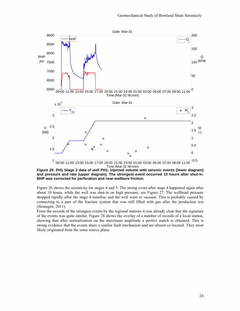
Geomechanical Study of Bowland Shale Seismicity
24
Figure 25: PH1 Stage 2 data of well PH1: injected volume with seismic events (lower diagram) and pressure and rate (upper diagram). The strongest event occurred 10 hours after shut-in. BHP was corrected for perforation and near-wellbore friction. Figure 26 shows the seismicity for stages 4 and 5. The strong event after stage 4 happened again after about 10 hours, while the well was shut-in on high pressure, see Figure 27. The wellhead pressure dropped rapidly after the stage 4 minifrac and the well went to vacuum. This is probably caused by connecting to a part of the fracture system that was still filled with gas after the production test (Stratagen, 2011). From the records of the strongest events by the regional stations it was already clear that the signature of the events was quite similar. Figure 28 shows the overlay of a number of records of a local station, showing that after normalization on the maximum amplitude a perfect match is obtained. This is strong evidence that the events share a similar fault mechanism and are almost co-located. They most likely originated from the same source plane.
09:00 11:00 13:00 15:00 17:00 19:00 21:00 23:00 01:00 03:00 05:00 07:00 09:00 11:006000
6500
7000
7500
8000
8500
9000
Time (Mar-31 hh:mm)
Date: Mar-31
0
50
100
150
200
BHPpsi
QBPM
BHP Qi
09:00 11:00 13:00 15:00 17:00 19:00 21:00 23:00 01:00 03:00 05:00 07:00 09:00 11:001
1.5
2
2.5
3
x 104
Time (Mar-31 hh:mm)
Date: Mar-31
-0.5
0
0.5
1
1.5
2
2.5
3
V(bbl)
M(-)
Vinj ML

2 Data Base
25
Figure 26: PH1 stages 4 and 5: injected and flowback volume with seismic events (lower diagram) and pressure and rate (upper diagram). The strong events after stage 4 occurred while the well was shut in with high pressure.
May-26 May-27 May-281
2
3
4
5
6
7x 10⁴
Time(mmm-dd)
-2
-1
0
1
2
V(bbl)
M(-)
Vinj
Vfb
ML
May-26 May-27 May-284000
5000
6000
7000
8000
Time(mmm-dd)
0
50
100
150
200
BHPpsi
QBPM
BHPBHPfb
Qi
Qfb
High pressure inFracture System

Geomechanical Study of Bowland Shale Seismicity
26
Figure 27: Zoom in on stage 4 in well PH1: injected and flowback volume with seismic events (lower diagram) and pressure and rate (upper diagram). The strong event after stage 4 occurred again about 10 hours after shut-in, as in stage 2.
Figure 28: Traces of seismic events vs time, observed on the local station HHF, normalized on maximum amplitude. The two upper diagrams show the horizontal components, which picked up the shear waves and the lower diagram shows the vertical component with the compressional wave. The records are remarkably similar in shape, showing that all events originated from the same source plane.
12:00 14:00 16:00 18:00 20:00 22:00 00:00 02:00 04:00 06:00 08:00 10:006000
6500
7000
7500
8000
Time (May-26 hh:mm)
Date: May-26
0
50
100
150
200
HPpsi
QBPM
BHPBHPfb
Qi
Qfb
12:00 14:00 16:00 18:00 20:00 22:00 00:00 02:00 04:00 06:00 08:00 10:001
2
3
4
5x 10⁴
Time (May-26 hh:mm)
Date: May-26
-2
-1
0
1
2
V(bbl)
M(-)
Vinj
Vfb
ML
11 11.5 12 12.5 13 13.5 14 14.5 15−1
−0.5
0
0.5
1
11 11.5 12 12.5 13 13.5 14 14.5 15−1
−0.5
0
0.5
1
11 11.5 12 12.5 13 13.5 14 14.5 15−2
−1
0
1
M1.5 05−27−00:48:45M1.2 05−26−22:35:58M0.7 05−26−23:06:01M0.5 05−27−14:21:27M0.4 05−26−14:39:27
Time (sec)

2 Data Base
27
Wellbore deformation Nature and extent of the deformation The Stage 2 (main) fracture treatment was conducted on March 31, 2011. Four days later, on April 4th, an obstruction was encountered at 8506ft when attempting to run in to the well with a bridge plug. A multifinger caliper log run on the 5th April encountered and quantified deformation of the casing. The limits of the interval of the casing deformation have been identified by two means. The upper limit was constrained when a 4⅝in mill was run in to 8273ftMD on the 12th July, 2011. The lower limit was defined by the multifinger caliper tool which started recording at a depth of 8734ftMD on the 5th April, showing minor deformation from the start of the run, see Figure 29. In summary, the upper limit is deeper than 8273ftMD and the lower limit deeper than 8734ftMD (Geosphere, 2011). This corresponds to a penetrated interval of not less than 461ft (140m) and a section normal to bedding of approximately 125m. Given the minor nature of the deformation at bottom of the logging run, 8734ft may be close to the maximum depth of the deformation but this possibility is not demonstrable. Figure 30 shows the casing deformation over the interval with a large deformation of more than 0.5 in. The severe deformation starts just below the Pendleside Limestone at the top of the Hodder Mudstone. The nature of the casing deformation is plotted as maximum and minimum radii in Figure 29. This figure shows that the deformation is very variable and essentially devoid of major offsets. Specialist software (Sondex) can be used to visualise the damage and this shows that the deformation ranges from barely detectable ovalisation to local buckling of the casing wall.
Figure 29: Minimum and maximum casing radius as measured over the deformed interval. The two passes (1,2) repeated fairly well.
3 4 5 68100
8200
8300
8400
8500
8600
8700
8800
MD
(ft)
D1-av, D1-max, D1-min, D2-av, D2-max, D2-min (in)
D1-avD1-maxD1-minD2-avD2-maxD2-min
0 50 100 150 2008100
8200
8300
8400
8500
8600
8700
8800
MD
(ft)
GRGC, GRGCfilt (gapi)
GRGCGRGCfilt

Geomechanical Study of Bowland Shale Seismicity
28
Figure 30: Variation of maximum and minimum casing radii derived from the 24arm caliper log from 8350‐ 8665ftMD in Well PH‐1. Three of the casing collar locations are also shown.There was some deviation over a very large interval, but more than 0.5 in ovalization occurs from 8500-8740 ftMD.
Figure 31: Azimuth of the least casing diameter for the interval 8400‐8670 ftMD in Well PH‐1 (pink dots). Since the fingers are spaced by 15o the azimuth shows digital noise by 15o. Bedding strike, interpreted from the image log, is plotted as a continuous blue line. Note that the azimuth is plotted only for a 0‐1800 range.
3.5 4 4.5 5 5.5 68350
8400
8450
8500
8550
8600
8650
8700
MD
(ft)
D1-av, D1-max, D1-min, D2-av, D2-max, D2-min (in)
D1-avD1-maxD1-minD2-avD2-maxD2-min
4000 4200 4400 4600 4800 50008350
8400
8450
8500
8550
8600
8650
8700
MD
(ft)
CCL ()
CCL
Pendleside Lst
Hodder Mst
Azimuth of min csg radius, deg (8400ft-8665ft)
8400841084208430844084508460847084808490850085108520853085408550856085708580859086008610862086308640865086608670
0 30 60 90 120 150 180
A z i m u t h , d e g
De
pth
,ft
MD
Azimuth ofminimum casedhole radiusStrike of bedding

2 Data Base
29
The displacement direction is indicated by the azimuth of the shortest radius of the caliper at each depth. A tool with 24 arms was used so the angular spacing between the “fingers” is 15o. This spacing, and the nature of the casing deformation, means that a plot of the azimuth of the shortest radius will commonly vary by perhaps 30o showing apparent steps of 15o. The variation of the azimuth of the minimum radius is shown in Figure 31, plotted with the strike of bedding. Figure 31 shows that the direction of transport trends parallel to the bedding strike (025o‐205o) and approximately 20o clockwise from the azimuth of the maximum horizontal stress. A rotation with depth (approximately 30o) is strongly inferred with an apparent discontinuity, interpreted as a thin limestone, at 8450 ftMD. (The logging contractor, Weatherford, confirmed that the observed rotation has not been attributed to an artefact of the logging process.)

Geomechanical Study of Bowland Shale Seismicity
30
3 Mechanism of Wellbore Deformation The temporal and spatial association of the recorded microseismicity with the hydraulic fracturing treatments is assumed to imply that the microseismic events were induced by the injection. A conceptual model of the geomechanics of the wellbore deformation can be proposed on the basis of the observations which are summarised above.
Casing deformation and the implications Comparison of the deformation shown in Figure 32 with a sample of the casing collar locations shows that casing deformation is not controlled by variations of the strength of casing. The variability of the magnitude of the deformation is a striking feature. There are a few examples of minimal deformation across limestone intervals (low gamma readings) such as at 8500ftMD. Changes in the magnitude of deformation are evident at many of the interfaces between a calcareous and a more argillaceous layer (e.g. at approximately 8480, 8505, 8575, 8560, 8600, 8605, 8610, 8620, 8630 and 8640ftMD).
Figure 32: Casing deformation overlain by Gamma ray (grey; x0.1). 3 casing collars are located.
MIT Max & Min diameters (Weatherford)
8450
8500
8550
8600
8650
8700
1
D i a m e t e r , i n
De
pth
,ft
MD
CSGJNT

3 Mechanism of Wellbore Deformation
31
Widespread tectonically‐induced casing ovalisation has been recognised and documented in variably‐dipping sandstones and shales (mainly shales) in the Eastern Cordillera of Colombia. Although the structural style is one of thrusting, stress determinations have revealed that the faulting environment in the Eastern Cordillera is strike slip. Last et al., (2002) reported that there are many examples of casing strings that have been ovalised, typically over several hundreds of feet. Last et al. (2002) reported that ovalisation is often small (just a few millimetres) and that the minimum casing diameter aligns with the maximum horizontal stress. Despite the fact that many of the wells cross active faults, the casing tends to ovalise and offsets of the casing by shearing are a rare occurrence. Although the magnitude of the ovalisation of the casing in Well PH‐1 is greater than that reported as typical by Last et al. (2002), the characteristic variability, extent and close proximity of the azimuth to the azimuth of the maximum horizontal stress are common features. The azimuth of the maximum reduction in casing diameter does not appear to correlate with the azimuth of channelling where indicated by the cement bond logs. The variability of the extent of ovalisation, often corresponding to high rates of change of the gamma ray readings, implies relative shear displacement on bedding planes.
Shear stress relief and interpretation of the discontinuities of the slip azimuth It was estimated that the fluid pressure gradient in the immediate vicinity of the wellbore during stimulation treatments were approximately 0.91 psi/ft (stage 1), 0.97 psi/ft (stage 2) and 0.91 psi/ft (stage 4). These gradients can be compared with the estimated total normal stress acting on bedding planes of various dips (Geosphere, 2011) bearing mind that the minimum horizontal stress has been estimated to range from 0.69‐0.77psi/ft. At such high pressures, bedding interfaces could be opened. Any bedding planes opened by the pressure of the injected fluid would experience zero resistance to sliding (other than small magnitudes that might be mobilised by any asperities where wall‐to‐wall contact happens to be preserved). In the presence of even very low magnitude shear stresses, bedding‐parallel slip would occur. That the variation of the azimuth of the minimum casing diameter (Figure 31) with depth, throughout intervals of more than 100ft, expressed as a progressive rotation, could speculatively be explained by quite smoothly progressive changes of intrinsic strength with depth. Given the heterogeneity and lithological variability of these sediments, smoothly progressive changes of intrinsic strength over such lengths are extremely unlikely. It is more likely that the rotation reflects progressive changes of effective normal stress and shear stress acting on the bedding planes. First, consider the variation of normal stress acting on the bedding planes. Assuming a constant reservoir pressure gradient, the deeper the horizon, the higher is the normal stress acting on the bedding planes. With this in mind, if a reason can be identified for the discontinuities in the rotation of the PH‐1 casing ovalisation azimuth (Figure 31), then an influence of normal stress might be identifiable. The discontinuities of azimuthal rotation occur at 8540ftMD and 8660ftMD. As will be discussed later, a pore pressure increase can be inferred to have been encountered starting at 8675ftMD. This would lower the effective normal stress and potentially weaken the resistance to bedding slip. No such pore pressure increase is inferred at 8540ftMD. Inspection of Figure 33 reveals a weak correlation between the interval of casing deformation and a bedding dip of 30‐35o. The aforementioned discontinuities at 8540ftMD and 8660ftMD approximately correlate with short intervals where the beds dip 19‐240. Slip has occurred parallel to the strike of the bedding (Figure 31). There is evidence for regional stress rotation (Geosphere, 2011), but even if the principal stress would be vertical, the presence of shear stress acting on subhorizontal surfaces is implied by the large stress differences. For bedding planes dipping westerly (subparallel to the axis of minimum horizontal stress), the higher the dip the less is the applied southerly directed shear stress. It appears, therefore, that while a reduction in the bedding plane strength might account for the discontinuity at 8675ftMD, only an increase the inferred shear stress is consistent with both of the discontinuities of the azimuth of maximum casing damage (8675ftMD and 8540ftMD). This implies that relief of the shear stress acting parallel to the strike of the bedding results in the observed rotation of the transport direction from parallel to the strike of bedding (25o) to parallel to the axis of maximum horizontal stress (estimated to be 7o). Bedding plane shear strength is also influential.

Geomechanical Study of Bowland Shale Seismicity
32
Figure 33: Minimum radius of the ovalised casing for the interval 8200‐8725ftMD and bedding dip (deg./10).
Conclusions The WNW-dipping bedding planes, almost certainly of all dip magnitudes, are subject to a bedding-parallel shear stress. This has been relieved to a variable extent by bedding plane slip. The magnitude of the shear stress acting on the bedding planes prior to drilling varied with depth prior to the PH-1 penetration. The transport direction associated with the casing damage is approximately parallel to the strike of bedding. Bedding-parallel relief of shear stress is associated with an anticlockwise rotation of the transport direction to align with the azimuth of the maximum horizontal stress. It is concluded that the nature and the extent of the casing deformation is a manifestation of distributed, small magnitudes of bedding plane slip. It has been possible only to conjecture a causal relation between the seismogenic slip and the wellbore displacements. In contrast, a very simple explanation, supported by core observations, has related the high-pressure fluid injections to slip at the wellbore. The outstanding questions are, first, whether the seismogenic activity resulted in any shearing of the wellbore at all and, if so, the relative magnitudes of the two categories of wellbore shear displacement.
Minimum RadiusBed Dip/10
Nominal Radius

4 Casing Deformation and Wellbore Integrity
33
4 Casing Deformation and Wellbore Integrity Following the 2.3 magnitude earthquake on April 1, Cuadrilla met with BGS to determine the best way to set up a seismic monitoring system for future fracture treatments, so that if any seismic events were incurred on future frac stages their position could be located with reasonable accuracy. When the recommended monitoring system was deployed preparations were made for conducting the Stage 3 fracture treatment. Cuadrilla attempted to run the zone isolation plug above the Stage 2 frac perforations. However, it was not possible to land the plug at the desired depth of 8550 ft. because the plug would not go down the wellbore past 8506 ft. A casing caliper tool was run and it was determined that the casing was deformed from a circular shape to an oval shape. The deformed interval was observed from approximately 8480 ft. to 8640 ft. The casing above and below that interval was not observed to be significantly deformed. Figure 34 shows a scale drawing of the deformed casing interval in the wellbore (deformed interval shown in YELLOW, near bottom of wellbore).
Figure 34: Casing Deformation in Preese Hall (vertically scaled drawing)

Geomechanical Study of Bowland Shale Seismicity
34
The initial field interpretation of the caliper survey (2 runs) suggested the casing ovalization was greater than what was actually observed from a physical measurement made for minimum casing diameter. A 3.25 inch tool was run on wire and passed easily through the deformed area and all the way down to the Stage 1 plug. So it was decided to return at a later date to attempt another caliper run, or possibly a camera run down through the deformed casing section, to get a clear understanding of the ovalization. While more analysis of the deformed area was forthcoming the initial caliper information was studied and it was determined that the deformed casing did not affect the overall wellbore integrity, and posed no risk to any shallow groundwater zones. As such, the decision was made to proceed with the Stage 3 fracturing treatment. Figure 35 shows the deformed casing interval in context with the wellbore integrity determination.
Figure 35: Casing Deformation in Context With Overall Wellbore Integrity (vertically scaled drawing for deformed interval plus perforated intervals)

4 Casing Deformation and Wellbore Integrity
35
In Figure 35 there is a RED solid line shown about halfway into the well. Everything above that RED line represents the portion of the well that protects the groundwater. In the upper part of the well is the 13-3/8” surface casing (cemented to a depth of about 1000 feet below the Sherwood Aquifer), and the 9-5/8” intermediate casing (cemented through the Manchester Marl which is the regional geologic seal). Below the solid RED line is section outlined in a BLUE box. This is the area of the well where we place hundreds of perforations in the 5-1/2” production casing in order to conduct our multi-stage frac program. This is a routine practice in oil and natural gas wells, both for conventional and unconventional reservoirs. In Figure 2 the groups of short, BLACK horizontal lines represent areas of the wellbore where the casing is already perforated (6 frac stages). The groups of short, RED horizontal lines represent areas where it is planned to place future perforations for up to 6 additional frac stages. (NOTE: at this point in time however, we may opt to only do 2 uppermost frac stages). From looking at the location of the deformed casing (YELLOW) it is clear that because of its location deep in the wellbore, and within the heavily perforated interval, it poses no more risk to the uphole wellbore integrity than the perforations themselves. For that reason we determined that we could proceed with our 3rd frac stage without any problems relating to the deformed casing.

Geomechanical Study of Bowland Shale Seismicity
36
5 Mechanism of seismicity Observations from various hydrocarbon and geothermal reservoirs indicate that shear slippage is the relevant mechanism for induced seismicity with magnitudes M>0 related to hydraulic treatments. These shear slip events are found to occur along existing failure planes such as faults, natural fractures, bedding planes and other discontinuities in rock (Warpinski et. al., 2006). Causing shear slippage by fluid injection is particularly utilized in geothermal reservoir development. In this context, extensive experience with respect to the associated induced seismicity was gained in numerous, massive stimulations of EGS reservoirs (Q-con, 2011). This type of seismicity exhibits characteristics that have also been observed during the hydraulic treatments in the Bowland Shale. The most important characteristics are:
• an increase of maximum magnitudes with time, • ongoing seismic activity after shutting in the well, • the largest magnitude events occur during shut-in.
Fluid injection induced seismicity is commonly described by the Hubbert-Ruby mechanism (e.g. Hubbert & Ruby, 1959; Healy et al., 1970; Hsieh and Bredehoeft, 1981), where hydraulic overpressures reduce the effective normal stress acting on existing fractures (or similar zones of weakness) until the ratio between shear- and effective normal stress exceeds the coefficient of friction and shear slippage occurs. Let τ and σn denote the shear and normal stresses resolved on a fracture plane, pfl the in situ fluid pressure, and μ the coefficient of friction, then shear slippage occurs on the fracture if:
n flpτ μ
σ>
− (1)
From equation 1 it follows that induced seismicity only occurs when several conditions are met:
1. Shear-stresses need to be resolved on the shearing plane, implying an anisotropic stress field. 2. The shearing plane needs to be mechanically strong enough to support high shear-stresses,
implying a significant strength of the associated rocks (rigidity). Furthermore, seismic energy is only released if the rigidity of the rocks is sufficiently large to allow for an almost instantaneous failure.
3. If fluid overpressures are the driving force for the induced seismicity, then the shearing plane must exhibit some natural hydraulic permeability.
It should be noted, that the Hubbert-Ruby mechanisms readily explains the occurrence of post-injection seismicity and the phenomenon of the largest magnitude events occurring after the treatment (Baisch et al., 2006). Another important factor is the dimension of the (naturally existing) shearing plane, which controls the magnitude of the associated earthquake. The strength of an earthquake can be described by the scalar seismic moment M0:
0M GAd= (2) Where G denotes shear modulus, A is the area of the shear plane, and d is the average slip occurring on the shear plane. Simple mechanical considerations reveal that the shear slip d cannot become arbitrary large, but is limited by:
- the capacity of the surrounding rock to absorb deformation, and - by the amount of shear stress driving the failure process.
Therefore, the dominating parameter controlling the magnitude of reservoir events is the area A of the associated shear plane. For an ML=2.3 earthquake, as observed in the Bowland Shale, the shear plane needs to be in the order of at least several 10,000 m2.

6 Maximum Magnitude of Future Seismic Events
37
6 Maximum Magnitude of Future Seismic Events A critical question in the framework of this study is whether or not future hydraulic treatments in the Bowland shale could produce similar or even stronger seismicity. The maximum earthquake magnitude is critically depending on the size of the stimulated reservoir (i.e. the penetration depth of hydraulic overpressures). For subsequent consideration we assume a similar treatment design, i.e. stage volumes of approx. 2,000 m3. Smaller injection volumes would lead to smaller earthquake magnitudes (Q-con, 2011). The numerical model has been used to estimate the maximum earthquake magnitude that could occur in the worst-case scenario. Since a number of parameters in the numerical model are not well constrained by observation data, different parameter combinations have been tested in order to match the observations. In the simulated parameter range, the maximum magnitude is predominantly influenced by the storage coefficient of the fault (Figure 36). The smaller the storage coefficient, the larger simulated event magnitudes become. The value of the storage coefficient is determined by porosity and thickness of the fault and the fluid (gas) compressibility. Assuming compressibility of water (cwater≈5 10-10 1/Pa), the best fitting model indicates a porosity-thickness product of φh=0.2 m, which is considered to be at the lower end of the realistic range. Assuming a larger compressibility (e.g. due to the presence of gas) further reduces the porosity-thickness product of the best fitting model. Therefore, we conclude that the storage coefficient is unlikely to be smaller than S=10-10 m/Pa. Although a good fit to observation data was only obtained for parameter combinations leading to Mmax=2.4, we note that in the parameter range considered possible, the maximum magnitude is ML=3.1 (Figure 36). We take this as an upper bound estimate for the maximum possible magnitude. Figure 36 shows the maximum magnitude simulated for various parameter combinations as a function of the parameter storage coefficient. A range of parameter combinations has been simulated in order to fit first order observations (pressure response and seismicity). Note that a systematic grid search through the parameter space is not feasible due to the large computation time required.
Figure 36: Maximum earthquake magnitude simulated in different numerical models assuming a different storage coefficient in the plane of weakness. Different symbols indicate to what extend simulation results match observation data. The best fitting model is indicated by a red square. Models consistent with observed hydraulic pressures and timing of the maximum magnitude event during shut-in are marked by red crosses. Note that data points of different models may plot at the same location. See text for details..

Geomechanical Study of Bowland Shale Seismicity
38
In the simulated range, the expected relationship between storage coefficient and Mmax can be observed (Figure 36). There is, however, not a strict relationship due to the multi-parameter nature of the simulations. For instance, numerical models with the same storage coefficient may lead to a different Mmax due to the variation of other model parameters. It should be noted that those models producing the largest magnitude events are not consistent with observation data (see different symbols in Figure 36). We have nevertheless used the entire set of simulations to obtain an estimate of the maximum earthquake magnitude for future treatments, which is in the order of ML=~3. This estimate is based on the assumption that the numerical models sufficiently sample the possible range of the model parameter space.

7 Potential for Upward Fluid Migration
39
7 Potential for Upward Fluid Migration In order to assess the risk of upward fluid flow we take the same approach as has been established for long term injection projects line Produced water Injection (OGP, 2000). For discussing confinement (i.e. keeping the fluid in a specified horizon), the first step is to define an area of review in which the different paths for upward fluid flow must be considered. The most obvious risk (but not always recognized) is the well itself or any nearby wells. The advantage is however, that wellbore integrity can be easily measured. In the PH1 well, there was poor cementing at the bottom of the well, but to upper section above 8000 ft depth had good cement, which provides good isolation of the treatment fluid. For evaluating risks from fractures and fault, we need to distinguish the Containment Layer which overlies the Injection Layer and the Confinement Layer which is above the Containment Layer. The shale gas appraisal wells will target the Worston and Bowland shales, which are therefore the Injection layers. The Millstone grit and Permian anhydrite can be considered the Containment Layer and Confinement Layer. There are two well-established mechanisms for containing fractures: high stress and permeable layers providing significant leak-off. There is evidence for a higher stress in the Millstone Grit from 6000-7000 ft. Also, the sandstone layers will provide some permeability for leak-off of the injected water.
Figure 37: Confinement of injected fluid inside the Injection Layer should be evaluated with respect to the Containment Layer (Millstone grit formation) and the overlying Confinement Layer.
Injection Layer
Containment Layer
Confinement Layer

Geomechanical Study of Bowland Shale Seismicity
40
The Millstone Grit is rather impervious, but even a small permeability in its sandstone members will quickly absorb water that would flow over a large distance through this formation. Two potential mechanisms should be considered: the hydraulic fractures propagated by the injections and any faults that may accept fluid. Injecting 15,000 bbl of water in a shale formation can propagate large fractures, but the size of the fracture is not unlimited. Although details of fracture propagation may be uncertain due to the heterogeneity of the rock formation, the principles of mass balance and elasticity will limit the maximum size of the fracture. This is different for injection into a fault where the storage capacity of the fault may change little with fluid injection. It is obvious that strong seismicity is likely associated with injection into a fault (as is extensively discussed in this report), so that raises the question where the fluid goes and how far it may migrate upward. Of most concern are then faults that extend to the surface, but these are not present in the Bowland. The Thistleton Fault is a very large fault, but it stops at the Permian anhydrite. Moreover, the well is at a sufficient distance from the fault, so it may be discarded from the review. For future wells, it would be important to consider any potential faults that are within a range of about 1000 ft so that fluid injection could reach such a fault. It is known that the Bowland is heavily fractured and faulted (which makes it a desirable target for shale get exploration), but these faults are relatively small and contained with the Bowland formation. One of these faults is the source of the seismicity. It must have a sufficient dimension in order to generate a seismic magnitude of 2.3 but that is at least 600 ft, which is still within the Bowland formation.
Figure 38: Stimulated zone after the end of the numerical simulation in plane view. Colors denote transmissibility values in the fault zone according to the color map. The highly stimulated area (white) extends laterally over a radius of approximately 1400 ft (425 m).

7 Potential for Upward Fluid Migration
41
Let’s now look at the extent of the fluid flow expected from the treatment volume. Obviously, it makes a big difference whether the injection takes a few hours (such as in stimulation treatments) or several years as in water or waste injection projects. From the fracture simulations (Stratagen, 2011) and hydro-mechanical fault injection simulations (Q-con, 2011), we know that the maximum extent in the worst case is about 1400 ft. Even with a safety factor of 50%, this would still fall within the Millstone Grit formation. So, it can be concluded that it is very unlikely that the fluid would ever leave the Containment Layer.

Geomechanical Study of Bowland Shale Seismicity
42
8 Seismic Hazard Related to Seismicity In tectonically active regions, house constructions frequently need to satisfy criteria specified by a local building code. In principle, such criteria could provide a guideline for estimating the level of ground motion above which damage might be expected. In the UK, however, such a building code does not exist. Compared to tectonically active regions, the earthquake hazard in the UK is low and thus only nuclear power stations are rigorously required to be designed and built to resist earthquakes (McCue et al., 2007). There exist numerous cases of damage caused by mining activities in the UK (e.g. Bell et al., 1988). The legal framework for damage compensation associated with mining is given by the Coal Mining Subsidence Act 1994 (chapter 21). The nature of mining damage caused by subsidence, however, is inherently different from damage associated with the transient ground shaking caused by reservoir seismicity. Although the case of man-made earthquakes is usually not explicitly covered by the law, experience with mining-induced earthquakes exists in many countries. In Germany, for example, the standard by which vibration impacts with regard to building damage are assessed is given by the German DIN4150-Part 3. (Effects of Vibration on Structure), which is summarized in Figure 39. In the UK, the corresponding standard is given by the British Standard 7385: Part 2 – 1993 (Evaluation and measurement for vibration in buildings Part 2: Guide to damage levels from ground borne vibration), which is summarized in Figure 40. Compared to the German DIN4150-3, the criteria in BS7385-2 are less stringent. It should be noted, however, that official guidelines regarding ground vibrations associated with blasting in the UK recommend more restrictive criteria. Therefore we follow a conservative approach by addressing the seismic hazard in light of the restrictive threshold values stated by the German standard DIN4150-3.
Figure 39 : Guideline values for peak particle velocity (mm/s) measured at the foundation of the building according to German DIN4150-3. Line 1 refers to buildings used for commercial purposes, industrial buildings and buildings of similar design. Line 2 refers to dwellings and buildings of similar design and/or use. Line 3 refers to structures that, because of their sensitivity to vibration, do not correspond to those listed in lines 1 and 2 and are of great intrinsic value (e.g. buildings that are under a preservation order).

8 Seismic Hazard Related to Seismicity
43
Figure 40: Guidance values for peak particle velocity (mm/s) measured at the base of the building according to BS 7385, part 2. Line 1 refers to reinforced or framed structures, industrial and heavy commercial buildings. Line 2 refers to unreinforced or light framed structures, residential or light commercial type buildings.
Figure 41: Peak ground velocity (PGV) as a function of distance for different signal frequencies according to the legend. PGV has been determined for an ML=2.6 earthquake at 3 km depth. Frequency dependent PGV threshold values according to DIN4150, line 2 (compare Figure 39) are indicated by dotted lines using the same color encoding. Note that the DIN4150 threshold value is reached by the 50 Hz curve (red line).

Geomechanical Study of Bowland Shale Seismicity
44
A relationship between earthquake magnitude and ground motion at the surface is provided by the classical definition of the Richter-Magnitude (ML; Richter, 1935). Due to local variations of the propagation properties of seismic waves, however, this relationship is location specific and needs to be calibrated for a specific region. Based on measured ground vibrations caused by the induced earthquakes in the Bowland Shale, the critical magnitude threshold above which slight material damage could occur according to DIN4150-3 has been determined as ML =2.6 (Q-con, 2011). In the past, mining induced earthquakes in the UK with magnitudes up to ML=3 caused no or only minor damage (Bishop et al., 1993). The associated earthquakes were located at shallower depth compared to the induced seismicity in the Bowland Shale. Since the amplitude of ground vibration on the Earth’s surface is larger for shallow earthquakes, we consider the threshold value determine here (i.e. ML=2.6) to be a conservative estimate.

9 Mitigation of the Magnitude of Seismic Events
45
9 Mitigation of the Magnitude of Seismic Events Several risk mitigation strategies have been developed in the course of this study. These include
• Reduction of the treatment volume (Q-con, 2011), • Aggressive flowback following hydraulic fracture treatments (Q-con, 2011), • Seismic real-time monitoring in combination with a “traffic light system”.
The seismicity occurred first during and after the second treatment stage, which was pumped immediately after the first stage, without any flow back of the well. In view of the low formation permeability, there is still a fairly high pressure in the well after the treatments. Also, the fourth stage showed significant seismicity and this stage was not flown back either. The third and fifth stage showed only weak seismicity, while there was aggressive flowback after these treatments. Figure 42 summarizes the injection and flowback volumes and the pressure at the end of the treatment and flowback. This observed correlation suggests that relief of pressure after the treatment can mitigate seismicity. Moreover, the effect is very well in line with the model, since there will be less injection of water into the fault if energy is taken out of the fracture system.
Figure 42: Injection volumes, flowback volumes and well head pressure after the flowback period for each treatment stage in well PH1. The most important measure is the operation of a traffic light system (Figure 43), which is based on the maximum acceptable magnitude ML,max=2.6 determined in the previous section. A complicating factor for the design of the traffic light system is the fact that the largest magnitude event tends to occur post injection. The maximum post-injection magnitude increase has been estimated to be 0.9 magnitude units (Q-con, 2011). Therefore, flow-back should be initiated at a magnitude level of ML=1.7 in order to prevent the occurrence of an ML,max =2.6 earthquake.
0
500
1000
1500
2000
2500
3000
3500
0
2000
4000
6000
8000
10000
12000
14000
16000
1 ‐mini 1 ‐main 2 ‐mini 2 ‐main before
3 mini
3 ‐mini 3 ‐main 4 ‐mini 4 ‐main 5 ‐mini 5 ‐main 6 ‐mini
WHP(psi)
Volume(bbl)
TremorsdVinj
dVfb
THP_end

Geomechanical Study of Bowland Shale Seismicity
46
Figure 43: Traffic light system proposed for future treatments in the Bowland Shale.
Statistical Traffic Light System Since the Bowland seismicity was observed in a single well and there is hard evidence that all events originated form a single fault, we have to rely on experience gained in other settings to make forecast for the seismicity in new wells. Of all possible mechanisms, we have identified fluid injection as the only credible mechanism that can explain the critical observations of the Blackpool seismicity, such as the magnitude and post-injection seismicity. We have based our estimate of maximum magnitude on the proposed physical process that induces the earthquakes. Based on a simplified model and experience in geothermal injections we have also estimated the maximum increase that could happen after shut-in. Although observations are consistent with the proposed physical mechanisms, the observation data is relatively sparse and some uncertainty about the mechanism remains. Another way to approach the remaining uncertainty is given by statistical methods. These are not based on a model of the physical processes but assume a certain distribution of earthquake magnitudes. Different statistical methods have been proposed to forecast earthquake probabilities during hydraulic treatment operations (Bachmann et al., 2011). In principle, these methods could be implemented into a traffic light system. The statistical methods, however, could be described as an adaptive filter where seismicity observed up to a certain point in time is used to predict the seismic activity for the following time window. In these approaches, the probability for a large magnitude event scales with the activity rate and quickly decreases in the post-injection period when the activity rate decays (e.g. figure 8 in Bachmann et al., 2011). For the data set discussed by Bachmann et al. (2011) we note that the statistical approaches failed to predict the occurrence of three M3 earthquakes occurring approximately 50-60 days after the injection (Deichmann & Giardini, 2009) during times of low seismic activity (Note that the time window in figure 8 of Bachmann et al., 2011 is restricted to 15 days and does not cover the time

9 Mitigation of the Magnitude of Seismic Events
47
window when the 3 M3 earthquakes occurred; the systematic decrease of the probability function with time, however, is evident already on the 15 day time window). These shortcomings of the probabilistic approaches have been noted in the course of a comprehensive risk study performed for the same data set (Baisch et al., 2009b). In contrast, the deterministic approach applied by Baisch et al. (2009b) – which is similar to the concepts used in this study - successfully explains the occurrence of these large magnitude, post-injection events. So, we conclude that the statistical approach is not applicable for the Bowland seismicity, since it is not conservative with regard to post-injection seismicity. On the other hand, the statistical analysis is way too conservative with regard to the upper limit of earthquakes that could be induced during injections. For estimating the maximum possible magnitude that could occur during injections, one might intuitively think that natural earthquakes might provide a reference frame. Although the Bowland is located in a region of very low natural seismic activity, we nevertheless note that the maximum possible magnitude for a natural earthquake in this region is probably in the order of ML6. Earthquakes of such large magnitude invoke a slipping plane with a length scale of 10 km. Clearly, stress perturbations caused by the hydraulic treatments considered here act on a much smaller length scale. Therefore, we feel that an upper bound estimate of Mmax based on natural earthquakes would be way too conservative.

Geomechanical Study of Bowland Shale Seismicity
48
10 Future Stimulation Treatments Although there is full confidence in the safety of operations in the PH1 well, it has been shown that weak seismicity still occurred in the fifth stage. Since the seismic events all originated from the same source plane this implies that the injected fluid could reach the seismic fault. Therefore it appears better to treat the new wells first. Even if the other wells would show similar, strong seismicity it is possible to conduct the stimulation treatments safely, with smaller treatments, aggressive flowback, a seismicity traffic light system based on monitoring of seismicity. However, it is quite likely that the new wells will show no strong seismicity at all. Therefore it is proposed to resume the stimulation treatments in the Grange Hill well. The programme will be modified with respect the PH1 well:
• The completion and workstring will be modified: The treatments will be pumped down the annulus, with a tubing in the well. The tubing will provide a dead string pressure measurement.
• Reduction of minifrac volumes: since water is more easily flowing into faults than slurry, the minifrac will be conducted for diagnostic purposes only. This would not require a volume of 700 bbl, but can be achieved with a smaller volume.
• The first treatment stages will be significantly smaller than the PH1 injection volumes. • After each stimulation treatment and minifrac, there will be release of fluid pressure in the
fracture system. • Seismic monitoring will be installed that can measure real-time any seismicity stronger than
magnitude ML=0. • A traffic light system will be employed ensuring mitigation of any seismicity.

11 Discussion and Conclusions
49
11 Discussion and Conclusions Subsurface engineering will always involve significant uncertainty, since there is limited data of processes occurring at great depth. The Preese Hall seismicity is no exception, since it occurred in a quite complex formation and involves a coupled process of fluid injection, fracturing and seismic failure of a large fault. Bounding the uncertainties requires that judgment is based on experience in similar projects and careful consideration of the geomechanical behaviour of the rock formations with state-of-the-art analysis of the observed data. One of the basic questions is whether the induced seismicity lends itself to such an analysis. If the slightest disturbance could trigger large earthquakes, any analysis would be hampered. However, such a scenario appears unrealistic, since it requires highly correlated stresses over large distances on a natural fault (Steacy & McCloskey, 1998). If this type of critically stressed fault would exist, then any small magnitude earthquake or other naturally occurring perturbation forces (e.g. solid Earth tides, load due to rainfall etc.) would trigger large magnitude earthquakes, which is not observed. Given that the seismicity does not depend on slight disturbances but rather falls in the category of ‘controlled’ induced seismicity, we need first of all to establish the driving force. There is no absolute certainty about the mechanism of the seismicity, since past experience shows that many processes have yielded seismicity. For instance, the opening of a fracture network by injecting water is expected to change the subsurface stress, which could induce fault slip. However, we have evidence from the timing of the seismicity and the remarkable similarity of the signals, that seismicity occurred on the same fault with pore pressure diffusion controlling the timing of the events. With the fluid volume injected during the hydraulic treatments, the area where in situ stresses are perturbed due to hydraulic overpressure is limited and is of similar size as required for a magnitude ML=2.3 earthquake. Therefore it can be concluded that direct injection into the fault must have induced the seismicity. Direct injection into a fault can be regarded as a worst case scenario, since stress perturbation caused by hydraulic overpressure is the dominating force. More indirect effects like short-ranging stress transfer could induce weak seismic events, which are of no interest in the context of the current study focusing on felt earthquakes. Let’s now look at the other key assumption in the hazard assessment, which is that the evolution of the seismicity can be controlled by operational parameters of the treatment (“well controlled scenario”). This assumption is based on a physical model and on experience made during numerous fluid injection operations (Q-con, 2011). In principle, the physical model also supports the occurrence of uncontrolled reactions (so called ‘butterfly’ effect), where even the smallest stress perturbation could lead to a large magnitude earthquake. Such effects can only occur if an existing shearing plane exhibits an extremely critical stress state over a large spatial area. Since the earth is never quiet (even in rural England), such super-critically stressed faults should yield also frequent natural earthquakes. Since earthquakes in Lancashire are rare we can be confident that the chance of triggering large earthquakes is negligible. In the current context, indications for an uncontrolled process may also be found by comparing the energy added to the system by hydraulic pumping to the energy released seismically. The seismic events are induced by the injections, but the energy is coming from tectonic strain energy in the rock formations. In this respect it is important to consider the ratio of energy provided by pumping to the energy released by the seismic slip. The energy ratio of the Blackpool seismicity is remarkably consistent with observations made in geothermal reservoirs, where seismic energy usually does not exceed 5% of the pumping energy. Thus, there is no indication for an uncontrolled process. Another observation is the remarkable similarity of the seismic records. This indicates not only a single source plane, but also that the same fault patch may fail repeatedly. This agrees with the picture of relatively small stress drops in the seismic slippages that are expected in the “controlled’ scenario. An important missing piece of evidence is the exact location of the seismic fault plane. It should be kept in mind that even if a fault plane had been identified in the image log or seismic section, this would not present hard evidence that this would be the source of the seismicity. It is only really possible to identify the slip plane if the seismic events had been accurately located. Evidence is offered that the likely fault plane is a so-called type A fault in Figure 8, which would be critically stressed, but this cannot be ascertained. If future treatments induce again seismicity it would be

Geomechanical Study of Bowland Shale Seismicity
50
important to determine whether the source is in the shale or rather the carbonate basement rock, but this is as yet uncertain. We presented evidence that the stage 2 scenario could be relatively close to a “worst-case-scenario” concerning the seismic hazard: Fluid was injected directly into an existing, critically stressed shearing plane which is large (and rigid) enough to host an ML=2.3 earthquake. Classifying this as a worst-case scenario would explain why earthquakes of similar strength have not been observed elsewhere during similar treatments (Q-con, 2011). Another critical assumption is the conceptual model of a pre-existing shearing plane intersecting the Preese Hall 1 well. However, details concerning the hydraulic coupling between the Preese Hall 1 well and the shearing plane through the different perforation intervals are unclear. In principle it is possible that the seismicity occurred on different, en echelon shearing planes intersected by Preese Hall 1. Without information on the spatial distribution of the induced seismicity (in particular, relative hypocenter locations) this hypothesis cannot be tested. We note, however, that the scenario of several shearing planes would not significantly change the results of the current study. In this scenario, the shearing plane associated with the stage 2 treatment would still be associated with a worst-case scenario. The physical processes and the maximum magnitude estimate would be the same as presented here. Since the Preese Hall stimulation treatments were the first in the Bowland Shale it seems natural to think that the Bowland must be special to explain that such unusual seismicity occurred. That inference would be correct if the induced seismicity in each stimulation stage would have come from different faults. However, there is strong evidence that the same fault was the source of all seismic events. Therefore, it cannot be concluded that all stimulation treatments are likely to cause unusual seismicity. We deal with just a single case and it is possible that this was just a very unlikely event that happened in the first try. An important factor is that experience from a large number of treatments in various settings show that it is quite unusual for hydro-frac injections to cause felt earthquakes. The proposed mechanism explains the rarity of the occurrence of the seismicity since a number of factors need to be satisfied: the well needs to be close to a critically stressed fault, which is also permeable and fails seismically. It is hard to estimate the likelihood of each of these factors, but the Carboniferous faults were formed a long time ago, so that only a fraction (say 10%) will be critically stressed by the current stresses. In fractured reservoirs, it is a common experience that out of the many observed fractures in an image log only a few are conductive in an injection test, say 1%. Seismic failure of faults is likely to depend on lithology and there are indications that the carbonate beds at the bottom of the Bowland Shale are very brittle and shear softening. However, the probability of seismic failure could be as low as 10%. The combined probability would then be one in ten thousand. This is obviously a crude estimate since we do not have specific evidence on fault permeability. We know from the drilling record of the well that no large mud losses were encountered. Also, the well was completely tight in a production test before stimulation, but there may be a large number of permeable faults, which could raise the probability to one in a hundred. Still, we conclude that the chance for a repeat of the felt seismicity is low. Conversely, if every well shows unusual seismicity, the assumptions behind the current modeling should be reconsidered. One of the necessary shortcomings of the employed model is that it is extremely simple. This is necessitated by the lack of detailed knowledge of the rock formations far from the well. On the one hand, modeling should avoid introducing many parameters that cannot be measured, while on the other hand the physical process must be captured. In the PH-1 well the seismicity involves both the failure of a large fault plane and the deformation of the wellbore, that both occurred in the second stimulation stage. The simplest explanation would have been that the fault slippage would have deformed the wellbore, but the large deformation zone can only be explained by extensive shear slip on bedding planes. It is unclear what the exact relation is between the seismic slip and the bedding plane slippage. Most likely, the seismic slip plane is not on a bedding plane with a small dip angle. The bedding plane shear could then be a precursor to the seismic slip and the shearing of the bedding planes could have opened a path for the slurry to the fault. It is also possible that the bedding shear was the result of the fault slip and should be regarded as secondary failure. The latter scenario would explain that the first stage did not induce seismicity nor any significant wellbore deformation, since the bridge plug could

11 Discussion and Conclusions
51
be run without any problem. It is believed that the wellbore deformation is not really essential for understanding the seismicity, but this illustrates that the entire process is quite complex. Given the complexity, it is best to restrict the analysis to the essential problem of the induced seismicity, which means that the opening of the fracture system as well as the borehole deformation were discarded from the numerical model. The fracture system might be close to a bi-wing fracture in view of the large horizontal stress difference, but it is likely that the fracture system is still rather complex because the net propagation pressure was high so that most joints and bedding planes can be opened by the high pressure. For the fluid injection into the fault, the main contribution from the fracture system is that it acts as a pressure baffle connected to the fault. Even long after shut-in this would have resulted in significant fluid injection into the fault, since flowing back the well took a long time before the pressure was relieved. Simplifying the model is not a big concern, since the diffusion of the fluid into the fault is a slow process. If there was still fluid flow into the fault after shut-in, the response of the pressure would be delayed, but the storage capacity of the fault would still determine the rate of pressure diffusion. Finally, it is important to consider the uncertainty in the maximum magnitude, given the uncertainties in the model. The model uncertainties have an impact on the size of the pressure disturbance, which controls the maximum magnitude. Since earthquake magnitude is measured on an amplified logarithmic scale (1 unit is a factor 32 in seismic energy), the gap between the observed magnitude of ML=2.3 and the estimate of the maximum magnitude of ML=3 is already a factor 11. This represents a robust safety factor and even if the estimated pressure distribution is uncertain, this will have a small impact on the estimated maximum magnitude. This is also apparent in the sensitivity of the maximum magnitude to parameters such as treatment volume. As expected, the magnitude decreases with halving the treatment volume, but only by 0.2, indicating that the estimate is robust and does not depend much on small deviations from the model assumptions.
Conclusions • The Bowland Shale consists mainly of impermeable, very stiff and brittle rock, with many
faults and fractures. • The horizontal stress in the Bowland shale is quite high, with a minimum stress gradient of
0.75 psi/ft and a maximum horizontal stress gradient of 1.25 psi/ft. With a vertical stress of 1.04 psi/ft, this is a strike slip stress regime with a large horizontal stress difference. The maximum horizontal stress orientation of 8o NNW agrees with the regional stress orientation.
• The structural dip of the bedding planes is quite high and variable. In the deformed zone the bedding dip is 35o, but in the bottom section it is 70-80o. Most likely, the pre-existing seismic fault is located near the transition between these zones.
o The orientation of this fault plane, dipping 70o towards the West with a strike of 20o NNE, agrees with the seismic interpretation and it would also be critically stressed.
• Apart from two seismic events that were reported by BGS (ML=2.3 and ML=1.5), 48 much weaker events were detected. The seismicity started during the first injection in stage 2. No seismicity occurred in stage 3, while stage 4 induced seismicity including the second strong event and stage 5 showed weaker seismicity.
o The strongest events occurred many hours after the injections and the signature of the seismic signals was remarkably similar. This is strong evidence that all events originated from the same fault and that the timing of the events was governed by the hydraulics of fluid flow into this fault.
o The absence of seismicity in stages 1 and 3 and the very weak seismicity during stage 5 can be explained by absence of fluid injection into the fault during these injections and by aggressive flowback of fluid after stages 3 and 5.
It is quite likely that sand in the fluid blocks off fluid injection into a fault with a small aperture.
Flowback releases energy stored in the pressurized fracture system, so that there is less energy remaining to induce seismic events.

Geomechanical Study of Bowland Shale Seismicity
52
• In order to determine the seismic source mechanism, recordings of a larger number of seismic stations is required. With only 2 stations available at the time of the induced seismicity, it is impossible to obtain a unique solution, but it has been confirmed that the observed ground motion agreed with the assumed strike-slip mechanism on a steeply dipping fault.
• Location of seismic events requires at least 4 stations. However, the local seismic stations show that the source of the events must be within 3000 ft from the injection interval.
• The temporal sequence of the events, with events starting during injection and shortly after injection while there was no seismicity at all before the injections and long after the injections, is clear evidence that the seismic events were induced by the fracture treatments.
• After stage 2, the casing was ovalized by more than 0.5 in over a long interval from 8500 to 8640 ftMD.
• Because of its location deep in the wellbore, the casing deformation poses no risk to the uphole wellbore integrity and the seal with respect to the overlying layers. For that reason, it is safe to proceed with stimulation treatments in the upper intervals.
• Stages 2 to 5 were traced with a chemical tracer so that the amount of flowback water could be measured for each stage.
o Assuming no retention of tracer, the overall flowback was about 20% of total injected fluid, while much of the flowback fluid was formation brine.
o Only a very small fraction of the stage 4 fluid was produced back to the surface. Most likely, the fluid entered a partially gas filled fracture system that was left after the production test.
Objectives and Conclusions Establish mechanism of seismicity
• Most likely, the repeated seismicity was induced by direct injection of fluid into the same fault zone. Slippage of the fault induced by high pressure occurred with the strongest events after the injection, since the pressure spread out over a larger area causing the largest event 10 hours after the injection in stage 2.
Estimate of maximum magnitude of seismic events induced by future fluid injection • Based on the seismic observations a simplified model was calibrated that predicts a maximum
event magnitude of ML=3 as a worst case. Evaluation of potential for upward fluid migration.
• In the worst case, the fluid could migrate upwards along a potential fault plane by 2000 ft. Because of the presence of a very thick impermeable formation overlying the Bowland shale and the Permian anhydrites that will act as barrier, there is negligible risk of fluid breaching into permeable layers.
Evaluate seismic hazard related to fault slippage in the target formation: what damage to surface structures could be done by a given event.
• Even the maximum seismic event is not expected to present a risk. In the UK area near Lancashire there have been many seismic events induced by mining induced seismicity that caused events up to magnitude ML=3.1 (Kusznir Bishop et al.,1980; Bishop et al., 1994; Lovell Bishop et al.,1997; Redmayne, 1988). Some of these events caused slight damage, but the seismic events originated from a depth of 1 km. At a depth of 3 km, these events may not have caused any damage.
• Based on the internationally accepted German standard for ground vibrations, a very conservative maximum seismic magnitude of ML=2.6 is adopted as the allowable limit to the seismicity. This ensures that no damage at all could be done to surface structures near a well that is fracture stimulated.
Mitigate the magnitude of seismic events. • From the observations and modeling we can identify two potential mitigation measures: rapid
fluid flow back after the treatments and reducing the treatment volume. Furthermore, intervals close to a fault (as identified with image logs) should be avoided.

11 Discussion and Conclusions
53
• Mitigation of seismicity can be achieved by monitoring seismicity during the treatments and taking appropriate action when seismic magnitude exceeds the limit set by the so-called traffic light system:
o Magnitude smaller than ML=0: regular operation o Magnitude between ML=0 and ML=1.7: continue monitoring after the treatment for at
least 2 days until the seismicity rate falls below one event per day. o Magnitude > ML=1.7: stop pumping and bleed off the well, while continuing
monitoring. • An important result from the identified mechanism is that measurable seismicity is unlikely to
occur in the next wells. The induced seismicity depends on three factors: presence of a critically stressed fault, a fault that is transmissible so that it accepts large quantities of fluid and a fault that is brittle enough to fail seismically. One of the reasons seismicity in propped fracture treatments is weak is that most fluid is pumped with significant sand concentration. Therefore it is likely that the slurry cannot easily enter a fault which will have a much smaller aperture than a hydraulic fracture. The seismic events imply that in the Preese Hall well a large fraction of the fluid entered a fault and this is one of the key factors that are unlikely to occur again in the other wells in the Bowland Shale.
• It is possible that the seismicity originated in the basement and that the hard limestone strata played a role in the seismicity. Future monitoring of treatments should resolve the depth location, which could help mitigating seismicity by avoiding injection into strata that are prone to strong induced seismicity.
References Attached detail reports Geosphere, (2011), “Geomechanical Analysis of Worston Shale Microseismicity”.
GMI, (2011), “Wellbore Failure Analysis and Geomechanical Modelling in the Bowland Shale, Blackpool, UK Cuadrilla Resources”, Final Report Submitted to Cuadrilla Resources, September 2011 Q-con, (2011), “Geomechanical Study of Blackpool Seismicity”.
Seismik, (2011), “Seismic analysis of the events in the vicinity of the Preese Hall well”
StrataGen, (2011), “Geomechanical Study of Bowland Shale Seismicity – Fracture Geometry and Injection Mechanism”.
General Arthurton, R.S. 1983 The Skipton rock fault–-an Hercynian wrench fault associated with the Skipton Anticline,
northwest England, 18 105-114
Arthurton, R.S. 1984 The Ribblesdale fold belt, NW England--a Dinantian-early Namurian dextral shear zone Geological Society, London, Special Publications 1984; v. 14; p. 131-138.
Bachmann, C. E., Wiemer, S., Woessner, J. and Hainzl, S. (2011), Statistical analysis of the induced Basel 2006 earthquake sequence: introducing a probability-based monitoring approach for Enhanced Geothermal Systems. Geophysical Journal International, 186: 793–807.
Baisch, S., Weidler, R., Vörös, R., and R. Jung, 2006. A conceptual model for post-injection seismicity at Soultz-sous- Forêts. Geothermal Resources Council, Trans., Vol. 30, 601-606.
Bell, F. G., Cripps, J. C., Culshaw, M. G., and M. A. Lovell, 1988. A review of ground movements due to civil and mining engineering operations. Engineering Geology of Underground Movements, Geological Society Engineering Geology Special Publication No. 5, pp. 3-32.
Bishop, I, Styles, P. and Allen, M. (1994). Mining Induced Seismicity in the Nottinghamshire Coalfield. Q. J. Eng. Geol. , 26 (4), 253-279.
Bishop, I., Styles, P., and M. Allen, 1993. Mining-induced seismicity in the Nottinghamshire Coalfield. Quarterly Jour. Eng. Geol., 26, 253-279.

Geomechanical Study of Bowland Shale Seismicity
54
Bungum, H., Vaage, S., and E. S. Husebye, 1982. The Meloy Earthquake Sequence, Northern Norway: Source Parameters and their Scaling Relations. Bull. Seism. Soc. Amer., 72(1), 197-206.
CBM Solutions, (2010), “Rock Mechanical Analysis For Cuadrilla Resources Preese Hall #1”, March 2010. Corfield, S.M., Gawthorpe, R.L., Gage , M, Fraser, A.J. and Besly, B.M. 1996 Inversion tectonics of the
Variscan foreland of the British Isles. Journal of the Geological Society, 153, 17-32.
Deichmann, N., and D. Giardini, 2009. Earthquakes induced by the stimulation of an enhanced geothermal system below Basel (Switzerland). Seis. Res. Let., 80, 784-798.
Redmayne, D. W., J. A. Richards and P. W. Wild (1998), Mining-induced earthquakes monitored during pit closure in the Midlothian Coalfield, Quarterly Journal of Engineering Geology & Hydrogeology; February 1998; v. 31; no. 1; p. 21-36.
Fairburn R. A. and Ferguson, J.1992. The characterisation of calcite‐filled fractures from the Northern Pennine Orefield. Proceedings of the Yorkshire Geological Society, 49, 117‐123,
Falcon, N.L. and Kent, P.E. Geological results of Petroleum Exploration in Britain 1945-1957 Geological Society of London memoir No.2, 63pp
Fraser, A. J., and R. L. Gawthorpe, 2003, An Atlas of Carboniferous basin evolution in northern England: Geological Society Memoir 28, 79 p.
Gawthorpe, R. L. 1986. Sedimentation during carbonate ramp-to-slope evolution in a tectonically active area: Bowland Basin (Dinantian), northern England. Sedimentology 33,185-206.
Gawthorpe, R. L., 1987, Tectono-sedimentary evolution of the Bowland Basin, northern England, during the Dinantian: Journal of the Geological Society (London), v. 144, p. 59–71.
Hanks, T. C. & Kanamori, H., 1979. A moment magnitude scale. Jour. Geophys. Res., 84, 2348-2350.
Hatherley, P., Styles, P, McKavanagh, B and Luo, X. (1995), Seismic Monitoring of Outburst and Rock Phenomena. in ' Management and Control of High Gas Emission and Outbursts in Underground Coal Mines', Lama, R., (Ed), Balkema: Rotterdam. 147-152.
Healy, J. H., Hamilton, R. M., and C. B. Raleigh, 1970. Earthquakes induced by fluid injection and explosion. Tectonophysics, 9, 205-214.
Healy, J. H., Hamilton, R. M., and C. B. Raleigh, 1970. Earthquakes induced by fluid injection and explosion. Tectonophysics, 9, 205-214.
Holland, Austin, (2011), “Examination of Possibly Induced Seismicity from Hydraulic Fracturing in the Eola Field, Garvin County, Oklahoma”, Oklahoma Geological Survey Open File Report OF1, 2011.
Hsieh, P. A., and J. D. Bredehoeft, 1981. A reservoir analysis of the Denver earthquakes: A case of induced seismicity. Jour. Geophys. Res., 86, 903-920.
Hsieh, P. A., and J. D. Bredehoeft, 1981. A reservoir analysis of the Denver earthquakes: A case of induced seismicity. Jour. Geophys. Res., 86, 903-920.
Hubbert, M. K., and W. W. Rubey, 1959. Role of fluid pressure in mechanics of overthrust faulting. Geol. Soc. Am. Bull., 70, 115-206.
Hubbert, M. K., and W. W. Rubey, 1959. Role of fluid pressure in mechanics of overthrust faulting. Geol. Soc. Am. Bull., 70, 115-206.
Kane, Ian A., Vicky Catterall, William D. McCaffrey and Ole J. Martinsen 2010 Submarine channel response to intrabasinal tectonics: The influence of lateral tilt AAPG Bulletin, v. 94, no. 2 (February 2010), pp. 189–219
Kusznir, N.J., D.P. Ashwin, A.G. Bradley, (1980), “Induced Seismicity in the North Staffordshire Coalfield, England”, Int. J. Rock Mech. Min. Sci. & Geomech. Abstr. Vol. 17, pp. 45 to 55.
Kusznir, N.J., D.P. Ashwin, A.G. Bradley, (1980), “Induced Seismicity in the North Staffordshire Coalfield, England”, Int. J. Rock Mech. Min. Sci. & Geomech. Abstr. Vol. 17, pp. 45 to 55.
Leeder, M R. 1988. Recent developments in Carboniferous geology: a critical review with implications for the British Isles band NW Europe. Proceedings of the Geologists’ Association, Vol. 99, 73–100.

11 Discussion and Conclusions
55
Lovell J.H., Henni P.H.O., Ford G.D., Baker C., I.G. Stimpson I.G. & Pettitt W., Recent Seismicity in the Stoke-on-Trent Area, Staffordshire. British Geological Survey Technical Report WL/97/27 1997. (Keele University)
Luza, Lawson, in: Nicholson, C., R.L. Wesson, (1990), “Earthquake hazard associated with deep well injection- A report to the US Environmental Protection Agency”, USGS 1951, Appendix A, p65.
McCue K. F., Musson R.M.W., and G. Gibson, 2007. A comparison of the seismicity of the UK and southeastern Australia. In AEES2007, The Australian Earthquake Engineering Society Conference, Wollongong NSW, 23 - 25 November 2007.
Moseley, F. 1953. Tthe Namurian of the Lancaster Fells. QJGS 109, 423-454
Moseley, F. 1962. The structure of the south-western part of the Sykes Anticline, Bowland, West Yorkshire. Proceedings of the Yorkshire Geological Society 33 , 287-314.
OGP, (2000), “Guidelines for Produced Water Injection”, Report No. 2.80/302
Redmayne, D.W. (1988) Mining induced seismicity in UK coalfields identified on the BGS National Seismograph Network. Geological Society, London, Engineering Geology Special Publications; vol. 5; pp. 405-413
Ren, T. X., D. J. Reddish and P Styles (2001) Numerical modelling and microseismic monitoring to improve strata behaviour. 29th APCOM April 25-27,2001,Bejing,P.R. China
Richter, C. F., 1935. An instrumental earthquake magnitude scale. Bull. Seism. Soc. Amer., 25 (1), 1-32.
Rutter, E., 2011a. First report, laboratory sliding friction tests, email to T.R. Harper, 24 August.
Rutter, E., 2011b. Second report, laboratory sliding friction tests, email to T.R. Harper, 9th September.
Steacy, S. J., and J. McCloskey, 1998. What controls an earthquake’s size? Results from a heterogeneous cellular automaton. Geophys. J. Int., 133, F11-F14.
Styles, P. Toon S. , and Bishop, I, (1994), Surface and borehole microseismic monitoring of mining induced seismicity: the potential for three dimensional fracture imaging, in 'Modern Geophysics in Engineering Geology, Liege, Belgium, 12-15 Sept. 1994, 395-408.
Styles, P. (1993). Implications of harmonic-tremor precursory events for the mechanism of coal and gas outbursts, in 'Rockbursts and Seismicity in Mines', Young, P. (Ed),Balkema, Rotterdam. 415-421.
Styles., P., , Toon., S. J. & Bishop. I., (1997), Surface and Borehole Microseismic Monitoring., Modern Geophysics in Engineering Geology, Geol Soc Spec. Pub 12, pp.315-326 .
Toon , S. M. and Styles, P., (1993), Microseismic Event location around long-wall coal faces using borehole, in-seam seismology, in 'Rockbursts and Seismicity in Mines', Young, P. (Ed), Balkema, Rotterdam. 441-444.
Warpinski, N. R., L. G. Griffin, E. J. Davis, & T. Grant, 2006. Improving hydraulic frac diagnostics by joint inversion of downhole microseismic and tiltmeter data. SPE 102690.
Waters, C.N,, Waters, R.A., Barclay,W.J. and Davies, J.R.2009. A lithostratigraphical framework for the Carboniferous succession of southern Great Britain (Onshore). British Geological Survey Research Report, RR/09/01

Geomechanical Study of Bowland Shale Seismicity
56
Figure 44: PH1 wellbore diagrams during the frac stages.
Figure 45: PH1 wellbore diagrams during the flow back periods. For the production test, a tubing was run.
7500
8000
8500
9000Enlarged Scale (-)
MD
(ft)
Frac Stages
Stage 1 Minifrac Stage 1 Frac Stage 2 Minifrac
Stage 2 FracStage 3 Minifrac Stage 3 Frac
Stage 4 Mini Frac Stage 4 Frac
Stage 5 Mini-Frac Stage 5 Frac
Stage 6 Mini-FracStage 6Stage 5Stage 4Stage 3Stage 2Stage 1
7500
8000
8500
9000Enlarged Scale (-)
MD
(ft)
Flowback Periods
before 3 mini
3-mini3-main-17/04 3-main 17/04-01/05 3-main 01/05 4-main 5-main 6-mini
Stage 6Stage 5Stage 4Stage 3Stage 2Stage 1

11 Discussion and Conclusions
57
Table 3: Overview of treatment dates, shooting of perforations, installing or milling of plugs and flowback periods. Treatment Perforations Plug Flowback
Stages Date Perf_date Top (ft) Bottom (ft)
Above zone date MD date_milled
4/Mar/11 8841 8850 Stage 1 Minifrac 26/Mar/11
27/Mar/11 8900 8909 27/Mar/11 8930 8939
Stage 1 Frac 28/Mar/11 None 1 29/Mar/11 8810 - 29/Mar/11 8730 8739 29/Mar/11 8750 8759 30/Mar/11 8700 8709
Stage 2 Minifrac 30/Mar/11 Stage 2 Frac 31/Mar/11
None 2 6/Apr/11 8495 17-Apr 6/Apr/11 8480 8489 7/Apr/11 8420 8429 7/Apr/11 8450 8459 Short flowback before stage 3 mini
Stage 3 Minifrac 8/Apr/11 Stage 3 Frac 9/Apr/11
Large flowback 3 23/May/11 8300 - 24/May/11 8020 8029 24/May/11 8120 8129 24/May/11 8250 8259
Stage 4 Mini Frac 25/May/11 Stage 4 Frac 26/May/11
Small flowback 4 26/May/11 8000 12/Jul/11 27/May/11 7810 7819 27/May/11 7900 7909 27/May/11 7970 7979
Stage 5 Mini-Frac 27/May/11 Stage 5 Frac 27/May/11
Large flowback 5 31/May/11 7800 11/Jul/11 31/May/11 7780 7789 31/May/11 7700 7709 31/May/11 7670 7679
Stage 6 Mini-Frac 31/May/11