geometallurgy – an overview of some … · geomet 2016 1 geometallurgy – an overview of some...

Geomet2016

1

GEOMETALLURGY – AN OVERVIEW OF SOME APPROACHES AND SOME REMAINING ISSUES

Peter Dowd

Acknowledgements Most of the work covered in this presentation has been conducted by members of the Mining Engineering Research Group at the University of Adelaide and, earlier, at the University of Leeds, with particular contributions from:

•  Assoc. Professor Chaoshui Xu (Adelaide) •  Stephen Coward PhD candidate (Adelaide) •  Exequiel Sepulveda PhD candidate (Adelaide) •  Dr Eulogio Pardo-Igúzquiza Research Fellow (Leeds)

Some of the work has been funded from various sources including: •  Newcrest Mining Ltd. •  Centre of Excellence in Mining and Petroleum Resources (SA State Gov.). •  QG. •  UK Engineering and Physical Sciences Research Council. •  UK Nirex Ltd.

Geomet2016

2

Overview •  Research issues in the quantification, modelling, estimation and

simulation of geometallurgical variables and their integration into resource and planning models.

•  In particular:

Ø  Extending traditional block models to to provide fully integrated approaches to mine design, planning and optimisation.

Ø  Predictive relationships for geometallurgical variables.

Ø  Non-additivity and upscaling.

Ø  Systems approaches to integrating geometallurgical models and downstream processes.

Ø  Sensed data.

Ø  Big data and rapid updating of resource models.

GEOMETALLURGY: EXTENDING TRADITIONAL BLOCK MODELS TO PROVIDE FULLY INTEGRATED APPROACHES TO MINE DESIGN, PLANNING AND OPTIMISATION

Geomet2016

3

Mine optimisation

•  A system is characterised by relationships among its components.

•  Optimising the individual components of a system does not optimise the system.

•  A mining operation is a system with a number of related components. •  For example, applying cut-off grades to mined ore lots to produce an

‘optimal’ production schedule does not necessarily optimise the entire mining operation.

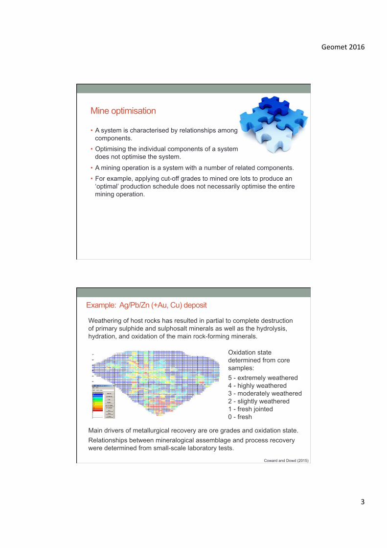
Oxidation state determined from core samples: 5 - extremely weathered 4 - highly weathered 3 - moderately weathered 2 - slightly weathered 1 - fresh jointed 0 - fresh

Main drivers of metallurgical recovery are ore grades and oxidation state. Relationships between mineralogical assemblage and process recovery were determined from small-scale laboratory tests.

Weathering of host rocks has resulted in partial to complete destruction of primary sulphide and sulphosalt minerals as well as the hydrolysis, hydration, and oxidation of the main rock-forming minerals.

Example: Ag/Pb/Zn (+Au, Cu) deposit

Coward and Dowd (2015)

Geomet2016

4

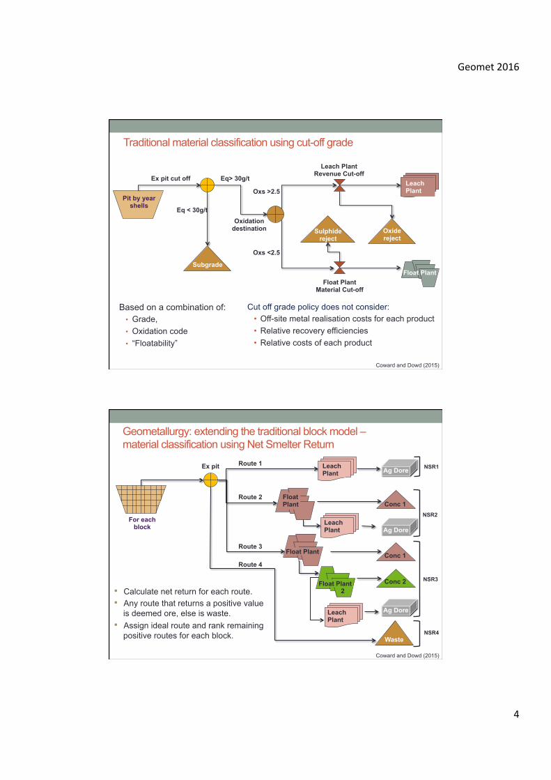
Traditional material classification using cut-off grade

Based on a combination of: •  Grade, •  Oxidation code •  “Floatability”

Subgrade

Eq> 30g/t

Eq < 30g/t

Ex pit cut off

Oxidation destination

Oxs <2.5

Oxs >2.5

Leach Plant Revenue Cut-off

Float Plant Material Cut-off

Oxide reject

Sulphide reject

Leach Plant

Float Plant

Cut off grade policy does not consider: •  Off-site metal realisation costs for each product •  Relative recovery efficiencies •  Relative costs of each product


Pit by year shells

Geometallurgy: extending the traditional block model – material classification using Net Smelter Return

•  Calculate net return for each route. •  Any route that returns a positive value

is deemed ore, else is waste. •  Assign ideal route and rank remaining

positive routes for each block.

Route 1 Ex pit

Float Plant Conc 1

Ag Dore

For each block Leach

Plant Ag Dore

Route 2

Waste Conc 1

Ag Dore

Route 3

Conc 2

NSR1

NSR2

NSR3

Waste

Route 4

Leach Plant

Leach Plant

Float Plant

Float Plant 2

NSR4


Geomet2016

5

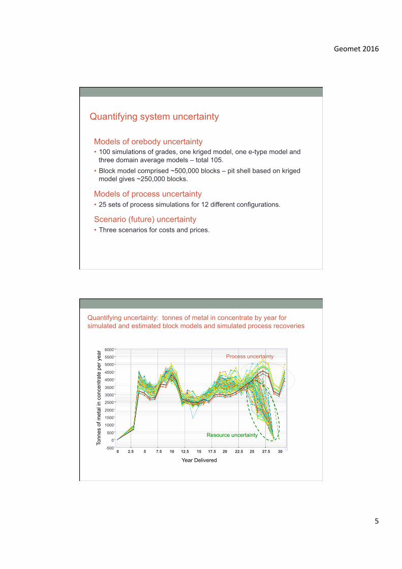
Models of orebody uncertainty •  100 simulations of grades, one kriged model, one e-type model and

three domain average models – total 105. •  Block model comprised ~500,000 blocks – pit shell based on kriged

model gives ~250,000 blocks.

Models of process uncertainty •  25 sets of process simulations for 12 different configurations.

Scenario (future) uncertainty •  Three scenarios for costs and prices.

Quantifying system uncertainty

Tonn

es o

f met

al in

con

cent

rate

per

yea

r

Year Delivered

0 2.5 5 7.5 10 12.5 15 17.5 20 22.5 25 27.5 30

6000

5500

5000

4500

4000

3500

3000

2500

2000

1500

1000

500

0

-500

Resource uncertainty

Process uncertainty

Quantifying uncertainty: tonnes of metal in concentrate by year for simulated and estimated block models and simulated process recoveries

Geomet2016

6

GEOMETALLURGY: PREDICTIVE RELATIONSHIPS FOR RESPONSE VARIABLES NON-ADDITIVITY

Successful geometallurgical modelling depends largely on the available data

§ Quantitative data for geometallurgical variables such as mineralogy, liberation profiles and particle size distributions are often not collected or are collected in insufficient numbers.

Solution: § Model geometallurgical response variables as a function of variables

for which there are abundant data (e.g., assays and geological logging).

§ Use an appropriate regression to derive an accurate prediction model.

But: § Relationships between primary input variables and geometallurgical

responses are, in general, complex and the response variables are often non-additive which further complicates the prediction process.

Multivariate linear regression performs poorly in such cases.

Geomet2016

7

Projection techniques

Objective: Detect relationships or structure in data sets: clusters, outliers, surfaces, linearity, non-linearity, skewness, . . .

•  For two-dimensional data sets (e.g., silver and lead core assays), structure and relationships easy to detect from a scatter plot.

•  More difficult for multi-dimensional data sets.

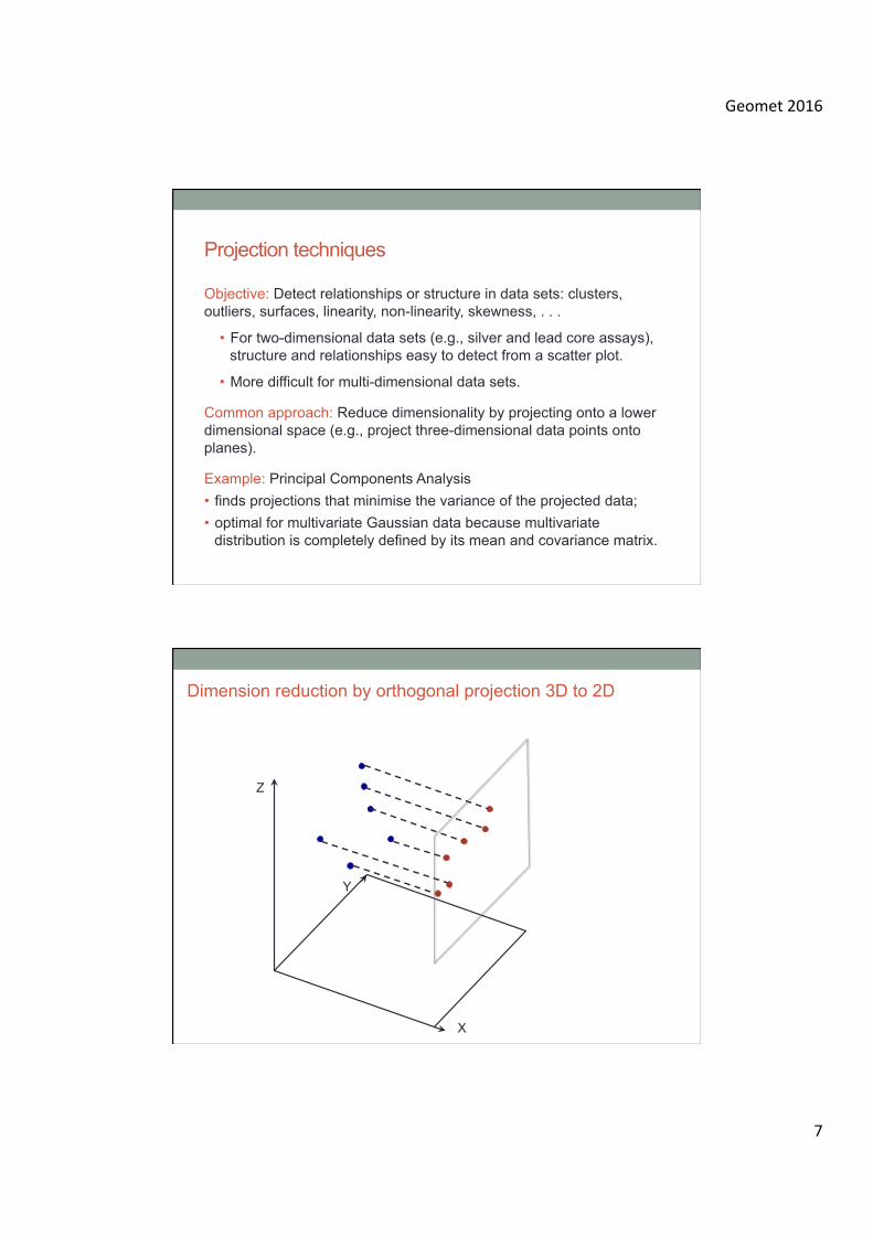
Common approach: Reduce dimensionality by projecting onto a lower dimensional space (e.g., project three-dimensional data points onto planes).

Example: Principal Components Analysis •  finds projections that minimise the variance of the projected data; •  optimal for multivariate Gaussian data because multivariate

distribution is completely defined by its mean and covariance matrix.

Dimension reduction by orthogonal projection 3D to 2D

Z

X

Y

Geomet2016

8

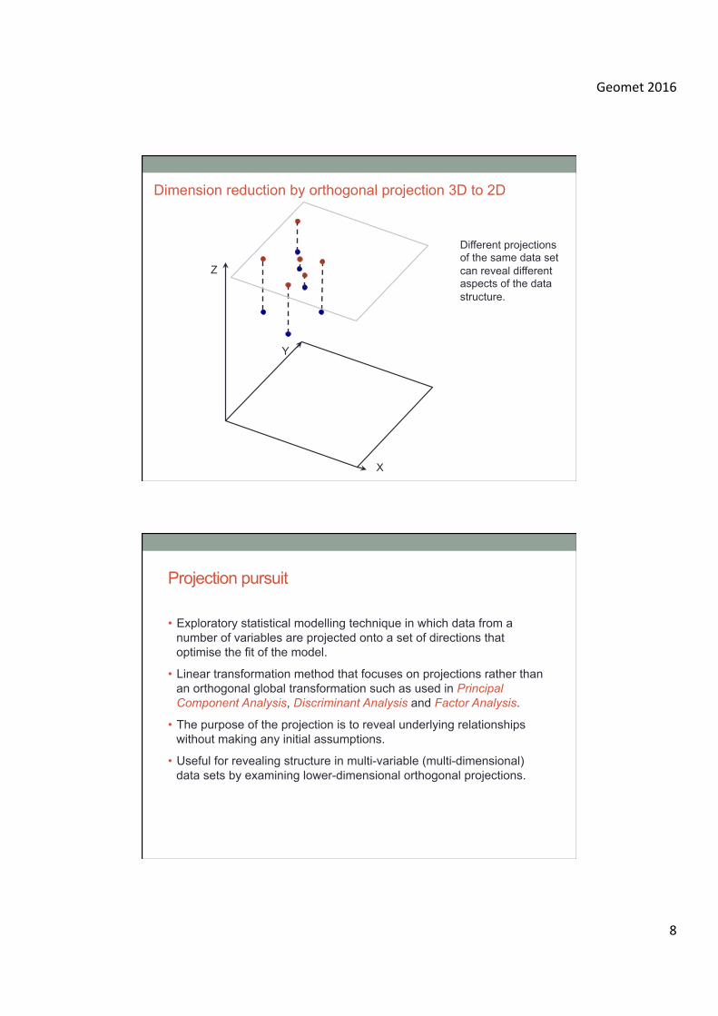
Dimension reduction by orthogonal projection 3D to 2D

Different projections of the same data set can reveal different aspects of the data structure.

Z

X

Y

•  Exploratory statistical modelling technique in which data from a number of variables are projected onto a set of directions that optimise the fit of the model.

•  Linear transformation method that focuses on projections rather than an orthogonal global transformation such as used in Principal Component Analysis, Discriminant Analysis and Factor Analysis.

•  The purpose of the projection is to reveal underlying relationships without making any initial assumptions.

•  Useful for revealing structure in multi-variable (multi-dimensional) data sets by examining lower-dimensional orthogonal projections.

Projection pursuit

Geomet2016

9

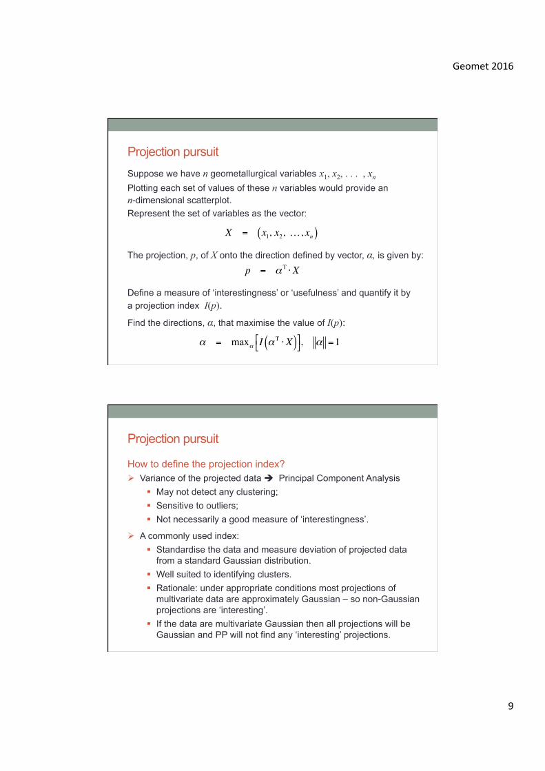
Projection pursuit Suppose we have n geometallurgical variables x1, x2, . . . , xn Plotting each set of values of these n variables would provide an n-dimensional scatterplot. Represent the set of variables as the vector: X = x1, x2, …, xn( )

The projection, p, of X onto the direction defined by vector, α, is given by:

p = α T ⋅X

Define a measure of ‘interestingness’ or ‘usefulness’ and quantify it by a projection index I(p). Find the directions, α, that maximise the value of I(p):

α = maxα I α T ⋅X( )⎡⎣

⎤⎦, α =1

Projection pursuit

How to define the projection index? Ø  Variance of the projected data è Principal Component Analysis

§  May not detect any clustering; §  Sensitive to outliers; §  Not necessarily a good measure of ‘interestingness’.

Ø  A commonly used index: §  Standardise the data and measure deviation of projected data

from a standard Gaussian distribution. §  Well suited to identifying clusters. §  Rationale: under appropriate conditions most projections of

multivariate data are approximately Gaussian – so non-Gaussian projections are ‘interesting’.

§  If the data are multivariate Gaussian then all projections will be Gaussian and PP will not find any ‘interesting’ projections.

Geomet2016

10

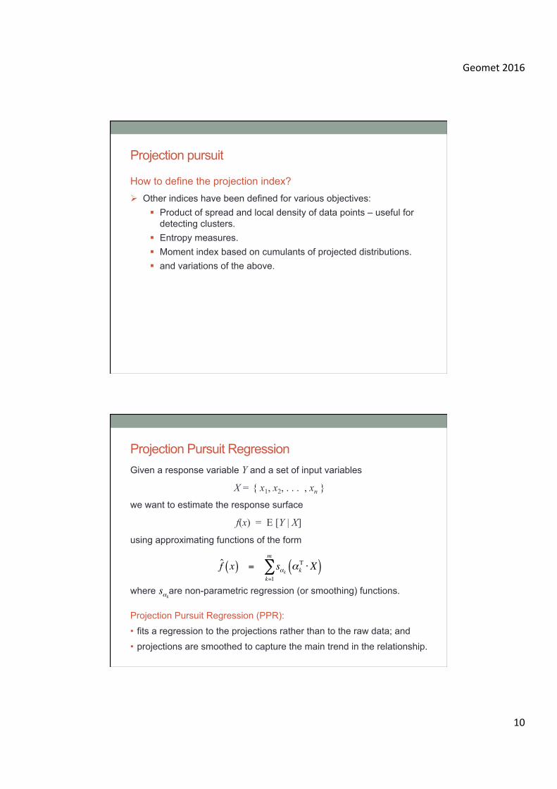
Projection pursuit

How to define the projection index?

Ø  Other indices have been defined for various objectives: §  Product of spread and local density of data points – useful for

detecting clusters. §  Entropy measures. §  Moment index based on cumulants of projected distributions. §  and variations of the above.

Projection Pursuit Regression

where are non-parametric regression (or smoothing) functions.

Given a response variable Y and a set of input variables

X = { x1, x2, . . . , xn } we want to estimate the response surface

f(x) = E [Y | X]

using approximating functions of the form

f̂ x( ) = sαk αk

T ⋅X( )k=1

m

∑

sαk

Projection Pursuit Regression (PPR): •  fits a regression to the projections rather than to the raw data; and •  projections are smoothed to capture the main trend in the relationship.

Geomet2016

11

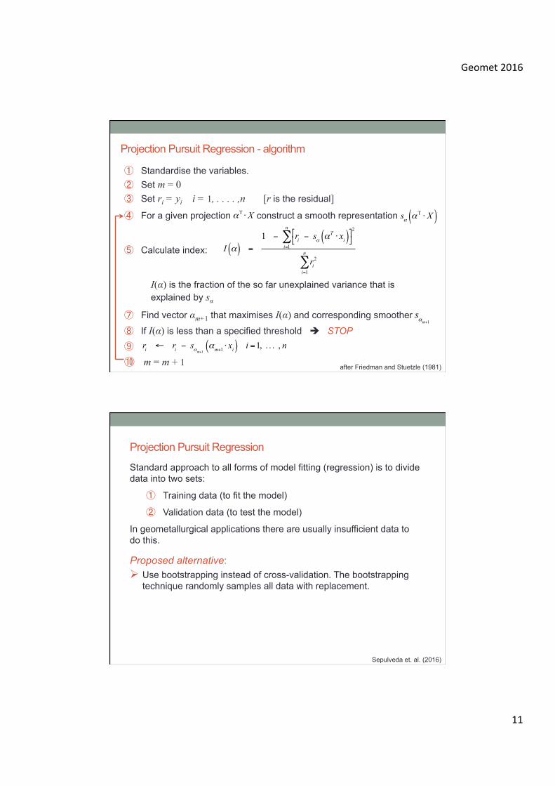
Projection Pursuit Regression - algorithm

①  Standardise the variables. ②  Set m = 0 ③  Set ri = yi i = 1, . . . . ,n [r is the residual] ④  For a given projection construct a smooth representation

⑤  Calculate index:

I(α) is the fraction of the so far unexplained variance that is explained by sα

⑦  Find vector αm+1 that maximises I(α) and corresponding smoother ⑧  If I(α) is less than a specified threshold è STOP ⑨  N

⑩  m = m + 1

ri ← ri − sαm+1 αm+1 ⋅ xi( ) i =1, . . . , n

αT ⋅ X sα αT ⋅ X( )

I α( ) =1 − ri − sα αT ⋅ xi( )#

$%&2

i=1

n

∑

ri2

i=1

n

∑

after Friedman and Stuetzle (1981)

sαm+1

Projection Pursuit Regression

Standard approach to all forms of model fitting (regression) is to divide data into two sets:

①  Training data (to fit the model)

②  Validation data (to test the model)

In geometallurgical applications there are usually insufficient data to do this.

Proposed alternative: Ø Use bootstrapping instead of cross-validation. The bootstrapping

technique randomly samples all data with replacement.

Sepulveda et. al. (2016)

Geomet2016

12

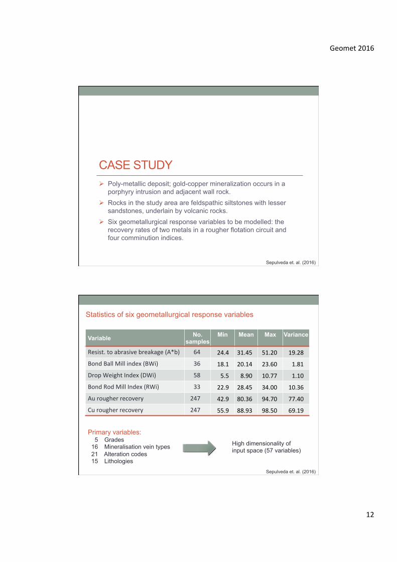
CASE STUDY Ø  Poly-metallic deposit; gold-copper mineralization occurs in a

porphyry intrusion and adjacent wall rock. Ø  Rocks in the study area are feldspathic siltstones with lesser

sandstones, underlain by volcanic rocks. Ø  Six geometallurgical response variables to be modelled: the

recovery rates of two metals in a rougher flotation circuit and four comminution indices.


Variable No. samples

Min Mean Max Variance

Resist.toabrasivebreakage(A*b) 64 24.4 31.45 51.20 19.28

BondBallMillindex(BWi) 36 18.1 20.14 23.60 1.81

DropWeightIndex(DWi) 58 5.5 8.90 10.77 1.10

BondRodMillIndex(RWi) 33 22.9 28.45 34.00 10.36

Aurougherrecovery 247 42.9 80.36 94.70 77.40

Curougherrecovery 247 55.9 88.93 98.50 69.19

Statistics of six geometallurgical response variables

Primary variables: 5 Grades

16 Mineralisation vein types 21 Alteration codes 15 Lithologies

High dimensionality of input space (57 variables)


Geomet2016

13

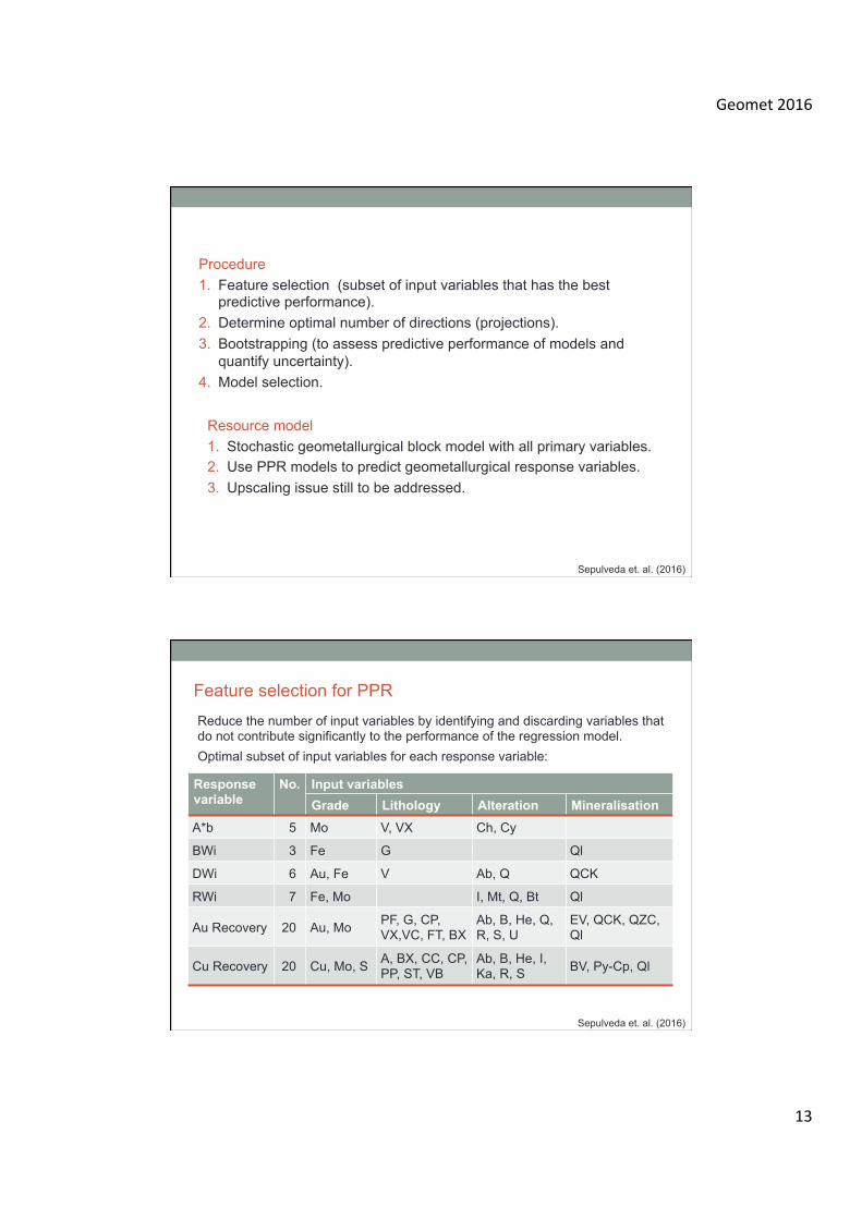
Procedure 1.  Feature selection (subset of input variables that has the best

predictive performance). 2.  Determine optimal number of directions (projections). 3.  Bootstrapping (to assess predictive performance of models and

quantify uncertainty). 4.  Model selection.


Resource model 1.  Stochastic geometallurgical block model with all primary variables. 2.  Use PPR models to predict geometallurgical response variables. 3.  Upscaling issue still to be addressed.

Feature selection for PPR

Response variable

No. Input variables Grade Lithology Alteration Mineralisation

A*b 5 Mo V, VX Ch, Cy

BWi 3 Fe G Ql

DWi 6 Au, Fe V Ab, Q QCK

RWi 7 Fe, Mo I, Mt, Q, Bt Ql

Au Recovery 20 Au, Mo PF, G, CP, VX,VC, FT, BX

Ab, B, He, Q, R, S, U

EV, QCK, QZC, Ql

Cu Recovery 20 Cu, Mo, S A, BX, CC, CP, PP, ST, VB

Ab, B, He, I, Ka, R, S BV, Py-Cp, Ql

Reduce the number of input variables by identifying and discarding variables that do not contribute significantly to the performance of the regression model. Optimal subset of input variables for each response variable:


Geomet2016

14

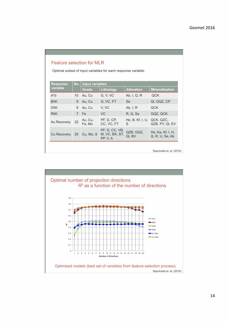
Feature selection for MLR

Response variable

No. Input variables Grade Lithology Alteration Mineralisation

A*b 10 Au, Cu G, V, VC Ab, I, Q, R QCK

BWi 9 Au, Cu G, VC, FT Se Ql, GQZ, CP

DWi 8 Au, Cu V, VC Ab, I, R QCK

RWi 7 Fe VC R, Q, Se GQZ, QCK

Au Recovery 22 Au, Cu, Fe, Mo

PF, G, CP, CC, VC, FT

He, B, Kf, I, U, S

QCK, QZC, QZB, PY, Ql, EV

Cu Recovery 25 Cu, Mo, S PF, G, CC, VB, M, VC, BX, ST, PP, V, A

QZB, GQZ, Ql, BV

He, Ka, Kf, I, H, Q, R, U, Se, Ab

Optimal subset of input variables for each response variable:


0

0.1

0.2

0.3

0.4

0.5

0.6

0.7

0.8

0.9

1 2 3 4 5 6 7 8 9 10 11 12 13 14 15 16 17 18 19 20

R2

Number of directions

A*b

BWi

DWi

RWi

Au Rec

Cu Rec

Optimal number of projection directions R2 as a function of the number of directions

Optimised models (best set of variables from feature selection process) Sepulveda et. al. (2016)

Geomet2016

15

0

0.1

0.2

0.3

0.4

0.5

0.6

0.7

0.8

0.9

1 2 3 4 5 6 7 8 9 10 11 12 13 14 15 16 17 18 19 20

R2

Number of directions

A*b

Bwi

Dwi

Rwi

Au Rec

Cu Rec

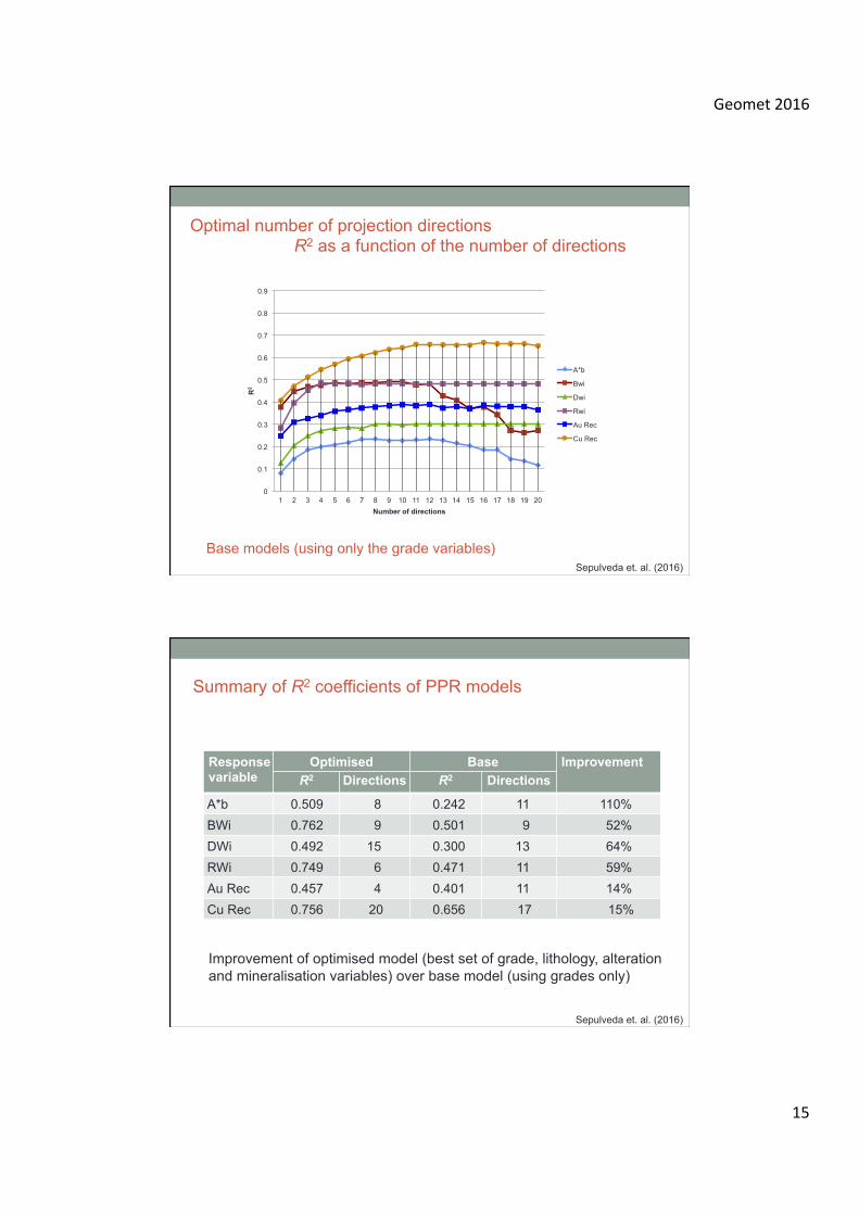
Optimal number of projection directions R2 as a function of the number of directions

Base models (using only the grade variables) Sepulveda et. al. (2016)

Response variable

Optimised Base Improvement R2 Directions R2 Directions

A*b 0.509 8 0.242 11 110% BWi 0.762 9 0.501 9 52% DWi 0.492 15 0.300 13 64% RWi 0.749 6 0.471 11 59% Au Rec 0.457 4 0.401 11 14% Cu Rec 0.756 20 0.656 17 15%

Summary of R2 coefficients of PPR models


Improvement of optimised model (best set of grade, lithology, alteration and mineralisation variables) over base model (using grades only)

Geomet2016

16

0.000

0.100

0.200

0.300

0.400

0.500

0.600

0.700

0.800

Ab BWi DWi RWi AuRec CuRec

Optimized PPR

Base PPR

Optimized MLR

Base MLR

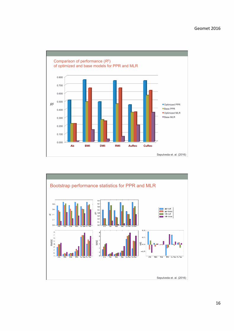
Comparison of performance (R2) of optimized and base models for PPR and MLR


R2

RM

SE

R

R2

MA

E

ME

Bootstrap performance statistics for PPR and MLR


Geomet2016

17

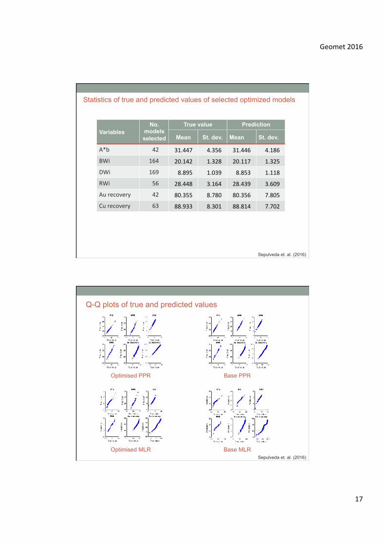
Variables No.

models selected

True value Prediction

Mean St. dev. Mean St. dev.

A*b 42 31.447 4.356 31.446 4.186

BWi 164 20.142 1.328 20.117 1.325

DWi 169 8.895 1.039 8.853 1.118

RWi 56 28.448 3.164 28.439 3.609

Aurecovery 42 80.355 8.780 80.356 7.805

Curecovery 63 88.933 8.301 88.814 7.702

Statistics of true and predicted values of selected optimized models


Q-Q plots of true and predicted values

Optimised PPR Base PPR

Optimised MLR Base MLR Sepulveda et. al. (2016)

Geomet2016

18

GEOMETALLURGY: Integration of geometallurgical models into mine planning, design and process optimisation.

Ø Current general approach to geometallurgical modelling: ü  identify the variables required to assess critical process responses; ü  find ways to sample and measure these variables; and ü develop techniques to estimate and simulate these variables

spatially at the correct scale and incorporate the values into block models.

Ø What is missing: •  Integration of the spatial geometallurgical model into a complete

mine systems model to quantify the impact of variable and uncertain rock properties on all stages of process performance, mine design and optimisation. è Integrated model of primary variables and response variables

and functions.

Geomet2016

19

Example: Classifying resource model blocks by breakage characteristics to improve coarse separation by optimal blasting and sorting by particle size.

1)  For given ore types, establish relationships between mineral occurrence, mineralogy, lithology, grade concentration and rock breakage/fragmentation characteristics by blasting or crushing.

2)  Establish relationships between relatively easily measured rock characteristics and the breakage/fragmentation of rock during blasting or crushing.

Ø  Examples: P32, geomechanical properties such as UCS, point load index, rock breakage test works such as drop weight index (DWi), crushing work index (CWi) or Hopkinson bar dynamic impact tests

Example: Classifying resource model blocks by breakage characteristics to improve coarse separation by optimal blasting and sorting by particle size.

3)  Develop/adapt blast models to predict post-blast fragmentation profiles of blasted material, as well as a rock primary crushing model for predicting fragmentation profiles.

4)  Develop an index (or, for complex rock type/mineralisations, a distribution of indices) for each resource block to quantify the extent to which sorting by particle size would improve feed grade.

5)  The forward modelling in (3) can be inverted to design blasts and/or to design a primary crushing circuit (in-pit or underground) to achieve a specified fragmentation profile (i.e., one that is optimal for sorting grade by particle size).

Geomet2016

20

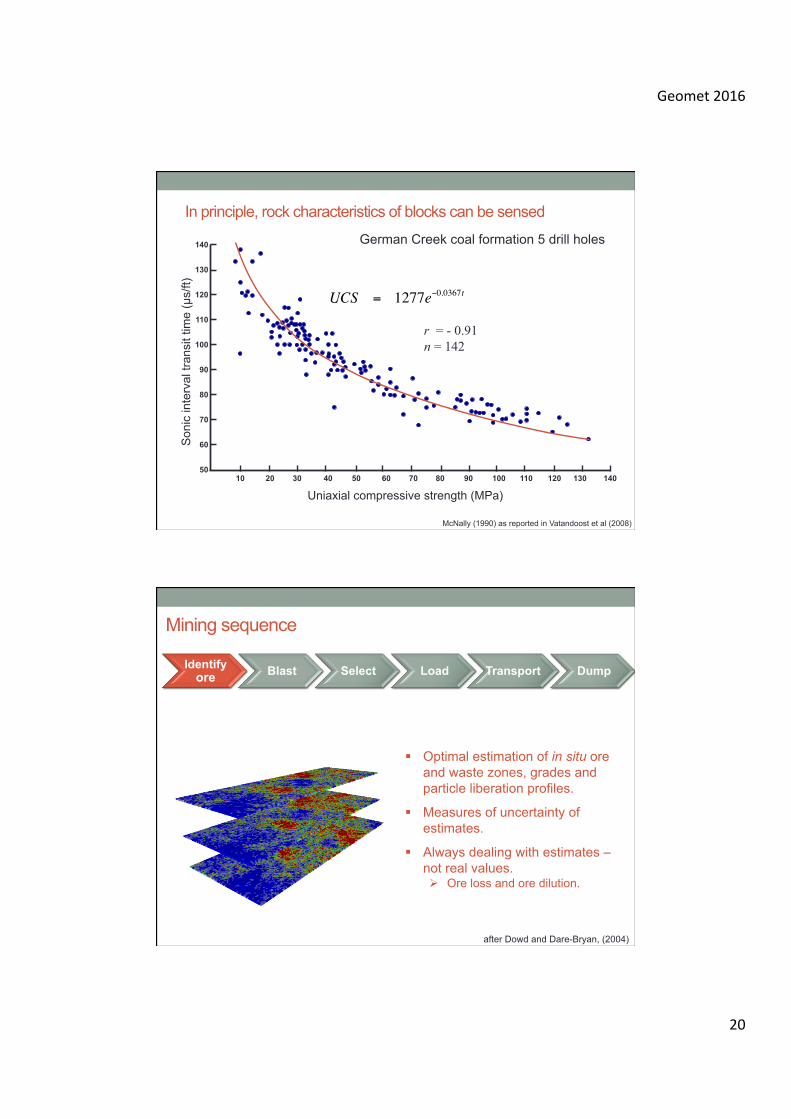
In principle, rock characteristics of blocks can be sensed

140

130

120

110

100

90

80

70

60

50 140 130 120 110 100 90 80 70 60 50 40 30 20 10

Uniaxial compressive strength (MPa)

Son

ic in

terv

al tr

ansi

t tim

e (µ

s/ft)

UCS = 1277e−0.0367t

r = - 0.91 n = 142

German Creek coal formation 5 drill holes

McNally (1990) as reported in Vatandoost et al (2008)

Identify ore Blast Select Load Transport Dump

§  Optimal estimation of in situ ore and waste zones, grades and particle liberation profiles.

§  Measures of uncertainty of estimates.

§  Always dealing with estimates – not real values. Ø  Ore loss and ore dilution.

Mining sequence

after Dowd and Dare-Bryan, (2004)

Geomet2016

21

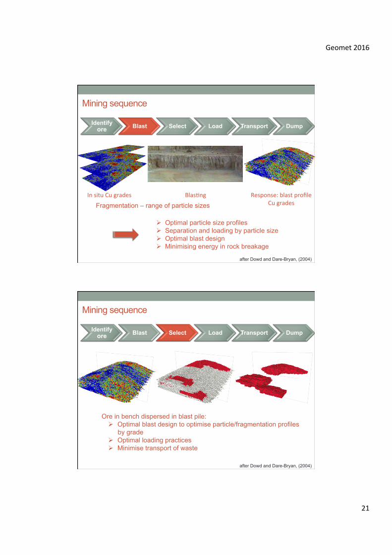
Mining sequence


Fragmentation – range of particle sizes

Ø  Optimal particle size profiles Ø  Separation and loading by particle size Ø  Optimal blast design Ø  Minimising energy in rock breakage

InsituCugrades BlasNng Response:blastprofileCugrades



Ore in bench dispersed in blast pile: Ø  Optimal blast design to optimise particle/fragmentation profiles

by grade Ø  Optimal loading practices Ø  Minimise transport of waste

Mining sequence


Geomet2016

22

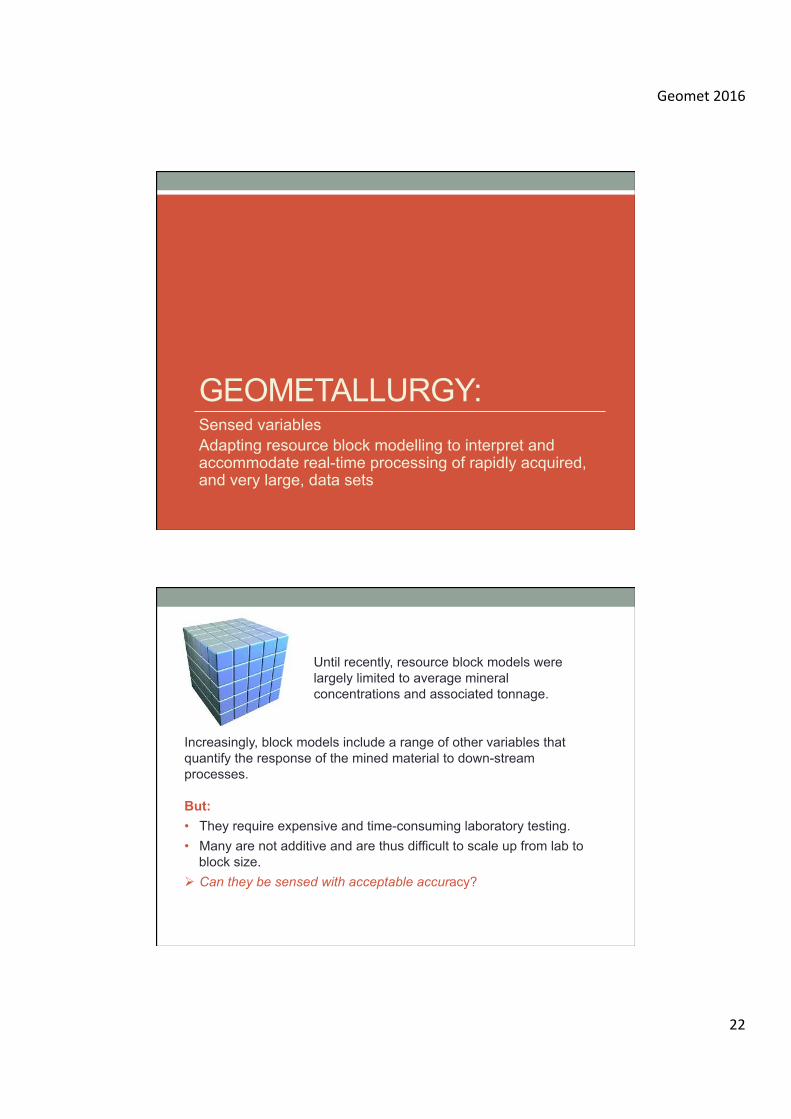
GEOMETALLURGY: Sensed variables Adapting resource block modelling to interpret and accommodate real-time processing of rapidly acquired, and very large, data sets

Until recently, resource block models were largely limited to average mineral concentrations and associated tonnage.

Increasingly, block models include a range of other variables that quantify the response of the mined material to down-stream processes. But: •  They require expensive and time-consuming laboratory testing. •  Many are not additive and are thus difficult to scale up from lab to

block size. Ø Can they be sensed with acceptable accuracy?

Geomet2016

23

Direct and sensed measurements

Ø  Shapes, physical boundaries, significant changes in characteristics §  Amenable to traditional forms of sensing. §  Tend to be (relatively) large-scale.

Ø  Mineral concentrations, geometallurgical variables •  Quantitative values that are measured on specific scales. •  Scale of measurement is relatively small; e.g. drill cores (cylinders of

rock of several cm diameter and typically from 1m to 10m in length depending on mineralisation and geology).

•  Variability of variables changes as scale of measurement changes – variability of a variable is inversely proportional to the volume on which it is measured.

•  Mineral concentrations are additive, many (most?) geometallurgical variables are not. Ø  Do not upscale (sample to block) linearly; spatial averaging may

have no meaning.

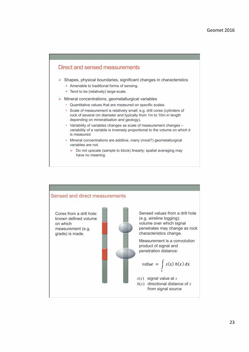
Cores from a drill hole: known defined volume on which measurement (e.g. grade) is made.

Sensed values from a drill hole (e.g. wireline logging): volume over which signal penetrates may change as rock characteristics change.

Measurement is a convolution product of signal and penetration distance:

s(x) signal value at x h(x) directional distance of x from signal source

Sensed and direct measurements

Geomet2016

24

Two approaches:

1)  Direct transform of the value of proxy (sensed) variable to the required direct variable.

2)  Indirect transform of the proxy variable by using implicit multivariate models of the (un-transformed) proxy variable and the required variable to predict values of the latter.

Ø  Calibration and integration of different types of data.

Promising approaches to direct transform of sensed variables

There is, for example, currently no general way of sensing in situ grade.

If the required information (e.g., grade) is in the signal, how can it be identified and extracted?

What can computer vision, automated recognition and artificial intelligence methodologies (e.g. deep learning) contribute?

Deep learning, convolutional neural networks have had remarkable success in many areas of automated recognition and in pattern and structure detection and can now significantly and consistently outperform humans.

Ø  Should perform very well in detecting shapes, boundaries, discontinuities in sensed geological/mine data.

Ø  Potential for quantitative data, such as grade?

Geomet2016

25

Data calibration and integration

•  Core samples measure direct values of variables over a known (specified) volume.

•  Sensed data are proxies for the direct values of variables; the sensed values are signal averages over an unknown volume that, in general, differs from the core volume. The sensed volume may change with location.

Ø For quantitative data, integration must address the volume-variance effect.

•  Use core values to calibrate signal values.

•  Data integration achieved by spatial co-variation models of direct and sensed data.

Example: Rock mass characterisation for the Sellafield Potential Repository Zone (PRZ) safe underground storage of low-level radioactive wastes

§  Borehole cores, wireline logs and 3D seismic survey data over the Sellafield PRZ.

§  Cores provide direct measurement of variables (e.g. porosity, permeability).

§  Wireline logs and survey data provide indirect measurements of varying quality (e.g. acoustic impedance).

Dowd (1997), Dowd, P.A. and Pardo-Igúzquiza, E. (2006, 2012)

Geomet2016

26

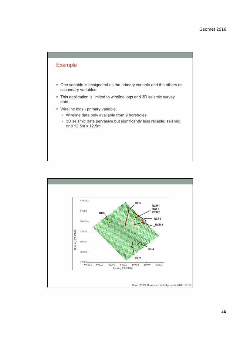
Example

§  One variable is designated as the primary variable and the others as secondary variables.

§  This application is limited to wireline logs and 3D seismic survey data.

§  Wireline logs - primary variable. •  Wireline data only available from 9 boreholes •  3D seismic data pervasive but significantly less reliable; seismic

grid 12.5m x 12.5m

BH5

BH2

BH4

BH5 RCM1 RCF3 RCM2

RCF1

RCM3

Easting (300000+)

Nor

thin

g (5

0000

0+)

4300.0

4100.0

3900.0

3700.0

3500.0

3300.0

3100.0 4800.0 5000.0 5200.0 5400.0 5600.0 5800.0 6000.0

Dowd (1997), Dowd and Pardo-Igúzquiza (2006, 2012)

Geomet2016

27

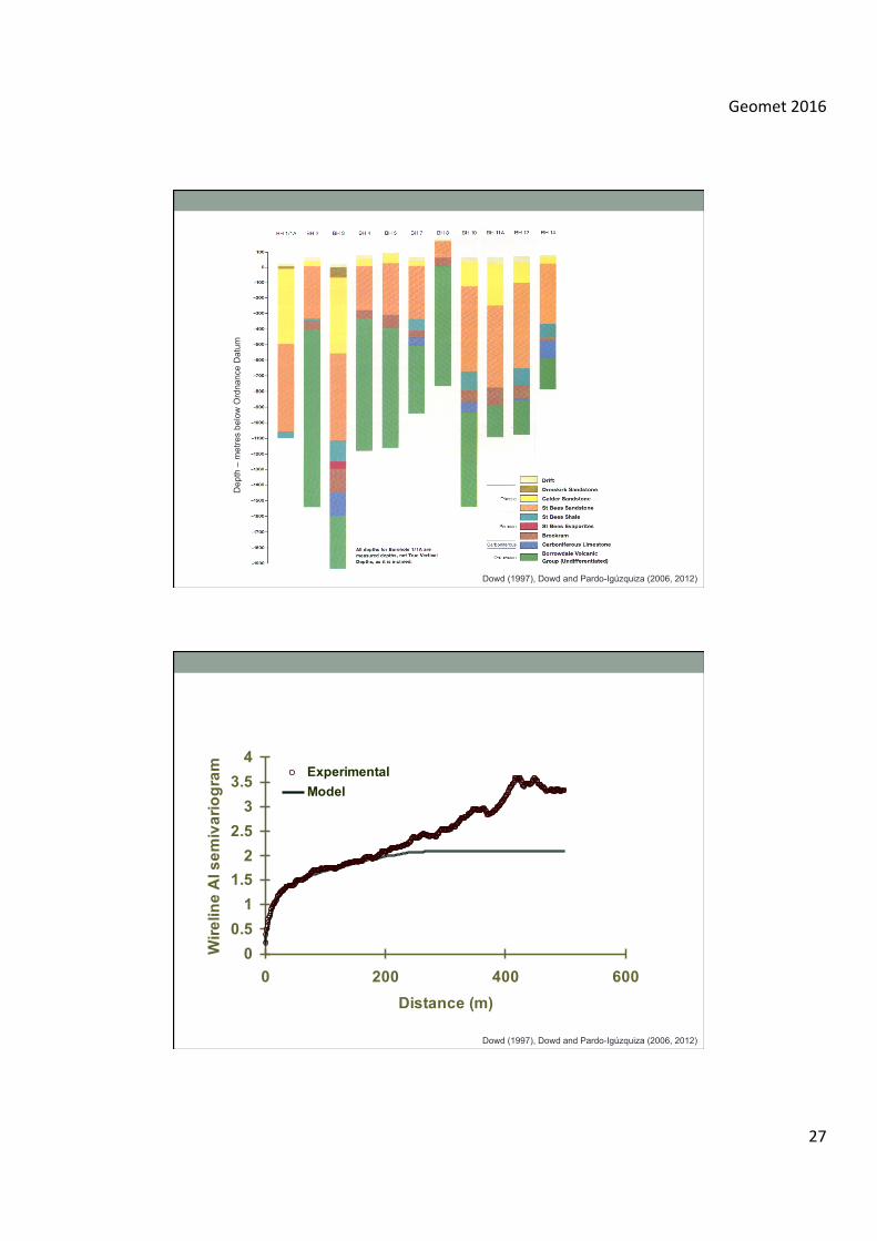
Dep

th –

met

res

belo

w O

rdna

nce

Dat

um


0

0.5

1

1.52

2.5

3

3.5

4

0 200 400 600

Distance (m)

Wir

elin

e A

I sem

ivar

iog

ram Experimental

Model


Geomet2016

28

0

0.2

0.4

0.6

0.8

1

1.2

1.4

1.6

1.8

2

0 100 200 300 400 500 600

Distance (m)

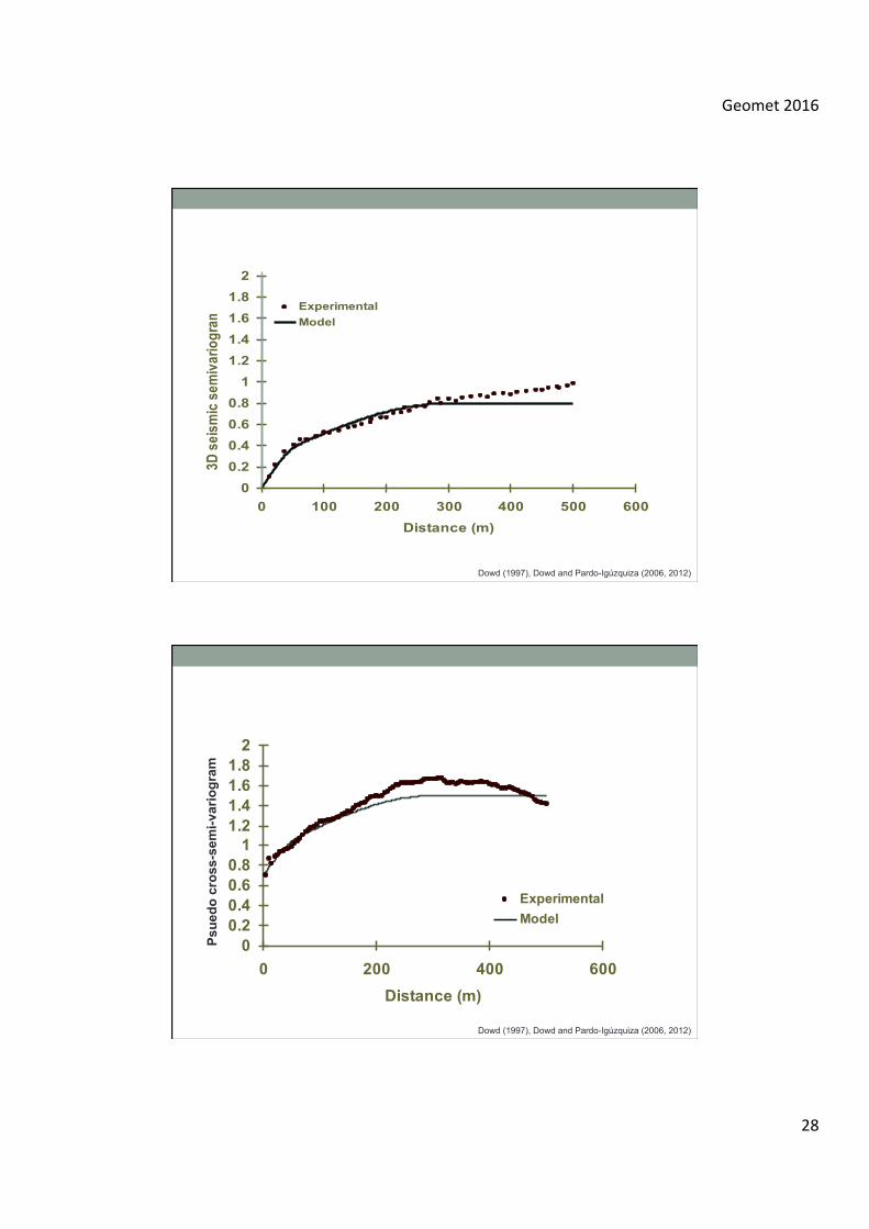
3D s

eism

ic s

emiv

ario

gram

ExperimentalModel


00.20.40.60.8

11.21.41.61.8

2

0 200 400 600

Distance (m)

ExperimentalModel

Psue

do c

ross

-sem

i-var

iogr

am


Geomet2016

29

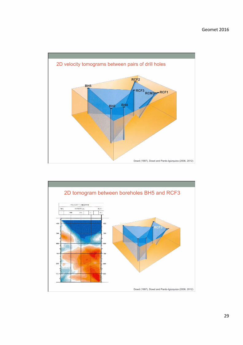
2D velocity tomograms between pairs of drill holes

BH5

BH2 BH4

RCF1

RCF2

RCF3 RCM3


BH5 RCF3

2D tomogram between boreholes BH5 and RCF3


Geomet2016

30

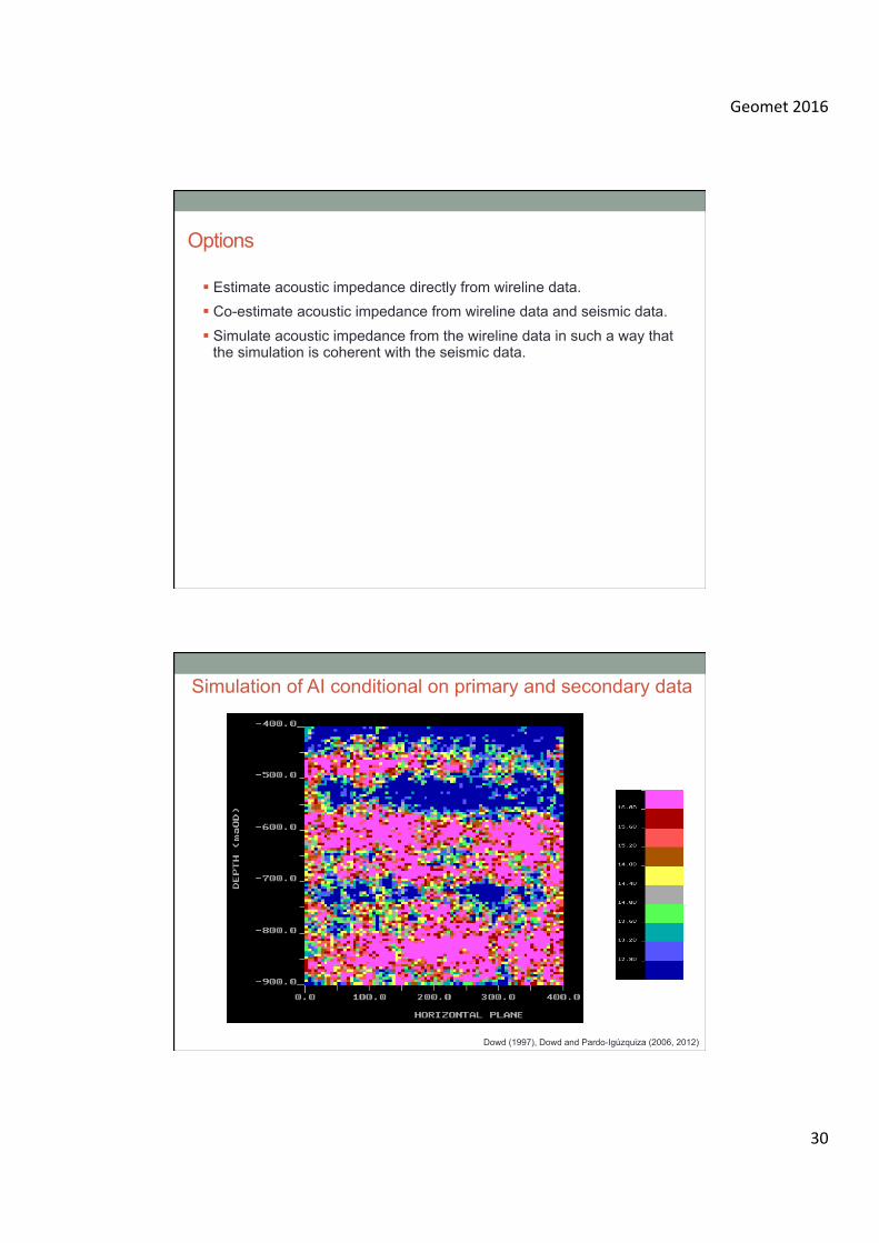
Options

§ Estimate acoustic impedance directly from wireline data. § Co-estimate acoustic impedance from wireline data and seismic data. § Simulate acoustic impedance from the wireline data in such a way that

the simulation is coherent with the seismic data.

Simulation of AI conditional on primary and secondary data


Geomet2016

31

OTHER RESEARCH ISSUES

Other research issues

•  Adapting resource block modelling to interpret and accommodate real-time processing of rapidly acquired, and very large, data sets.

•  Complete resource block models can be very large:

Ø  several million blocks with up to 20 variables in each (possibly many more with sensed data).

•  Resource modelling can be extensive and computationally intensive:

Ø  Estimation and co-estimation of many variables;

Ø  Multiple (100+) simulations of block variables;

Ø  Can model updates be limited to the zones for which new data are acquired?

•  How to interpret sensed geometallurgical data (convert signal to required variable on the correct scale)?

Geomet2016

32

Three characteristics of big data

1.  Multiple, distributed sources •  ‘Hard” data and on-line sensing

2.  Automation •  Analyse data as they are collected

3.  Feedback •  Return results to the system and update the system

References Coward, S., Dowd. P.A. and Vann, J. (2013) Value chain modelling to evaluate geometallurgical recovery factors. Proceedings of the 36th APCOM Conference; pub. Fundação Luiz Englert, Brazil; ISBN 978-85-61155-02-5; 288-289. Coward, S. and Dowd. P.A. (2015) Geometallurgical models for the quantification of uncertainty in mining project value chains. Proc. 37th APCOM Conference; Soc. Mining, Metallurgy and Exploration ISBN 978-0-87335-417-2; 360-69. Dowd, P.A. (1997). The geostatistical characterization of three-dimensional spatial heterogeneity of rock properties at Sellafield. Trans. Instn. Min. Metall.,106, A133-147. Dowd, P.A. and Dare-Bryan, P.C. (2004) Planning, designing and optimising using geostatistical simulation. Proceedings of the International Symposium on Orebody Modelling and Strategic Mine Planning. Pub AusIMM (Melbourne). ISBN 1 920806 22 9; 321-338. Dowd, P.A. and Pardo-Igúzquiza, E. (2006) Core-log integration: optimal geostatistical signal reconstruction from secondary information. Applied Earth Sciences, 115, (2), 59-70. Dowd, P.A. and Pardo-Igúzquiza, E. (2012) Integration of spatial geophysical data by geostatistical simulation. Z. Geol. Wiss., Berlin 40, (4/5): 267 – 280. Friedman, J.H. And Stuetzle, W. (1981) Projection pursuit regression. J. Amer. Stat. Assoc., 76 (376),817-823. McNally, G.H. (1990). The prediction of geotechnical rock properties from sonic and neutron logs. Exploration Geophysics, 21, 65-71. Sepulveda, E., Dowd, P.A., Xu, C. and Addo, E. (2016) Multivariate modelling of geometallurgical variables by projection pursuit. Under review for Mathematical Geosciences. Vatandoost, A., Fullagar, P. and Roach, M. (2008) Multi-sensor petrophysical core logging: Data acquisition, processing and preliminary interpretation of Cadia East data. GeMIII (AMIRA P843) Technical Report 1, 4.1-4,31.

geometallurgy – an overview of some … · geomet 2016 1 geometallurgy – an overview of some...

Documents