geometric descriptions of couplings in fluids and...
TRANSCRIPT

Geometric Descriptionsof
Couplings in Fluids and Circuits
Thesis by
Henry O. Jacobs
In Partial Fulfillment of the Requirements
for the Degree of
Doctor of Philosophy
California Institute of Technology
Pasadena, California
2012
(Defended April 20, 2012)

ii
c© 2012
Henry O. Jacobs
All Rights Reserved
iii
to the memories of
Manuel Jacobs,
Chin Hyung Kim,
and Jerrold E. Marsden

iv
Acknowledgements
I was only able to work with Professor Marsden for two years. However, I continue
to learn from him well after his death. While it is obvious this research stands on his
intellectual shoulders, there is a larger statement to be made in regards to his warmth.
Upon Jerry’s passing I found myself caught by a supportive family of researchers. My
new advisor, Mathieu Desbrun, has taken great care of me by providing useful advice
on how to direct my research, while simultaneously supporting all of my ventures.
Additionally, Melvin Leok and Hiroaki Yoshimura provided me with much-needed
encouragement and moral support upon Jerry’s death.
Secondly, I would like to thank Hiroaki Yoshimura, Tudor S. Ratiu, and Alan
Weinstein. Each took substantial risk in adopting me as a collaborator, and spent a
good deal of time reading early drafts of our work and getting me past some major
obstacles in my research.
Finally, I owe thanks to a variety of individuals who helped in ways big and
small: Chris Anderson, Andrea Bertozzi, Sam Burden, Martins Bruveris, Joel Bur-
dick, Alexandre Chorin, Fernando de Goes, Dennis Evangelista, Humerto Gonzales,
Darryl D. Holm, Matthew Inkman, Kaushik Jayaram, Eva Kanso, Erica J. Kim,
Marin Kobilirov, Richard Montgomery, Patrick Mullen, Richard Murray, Sujit Nair,
Clara O’Farrell, Tomoki Ohsawa, Houman Owhadi, Shankar Sastry, Michael J. Shel-
ley, Paul Skeritt, Hui Sun, Yoshihiro Shibata, Molei Tao, Cesare Tronci, Tomasz
Tyranowski, David Uminsky, Arjan Van DerSchaft, Joris Vankerschaver, Ram Va-
sudevan, Thomas Werne, Jon Wilkening, Tomohiro Yanao, and Yu Zheng.
Finally, I would like to thank my family, my wife, and my wife’s family for sup-
porting me in all the ways that families can.

v
Abstract
Geometric mechanics is often commended for its breadth (e.g., fluids, circuits, con-
trols) and depth (e.g., identification of stability criteria, controllability criteria, con-
servation laws). However, on the interface between disciplines it is commonplace
for the analysis previously done on each discipline in isolation to break down. For
example, when a solid is immersed in a fluid, the particle relabeling symmetry is bro-
ken because particles in the fluid behave differently from particles in the solid. This
breaks conservation laws, and even changes the configuration manifolds. A second
example is that of the interconnection of circuits. It has been verified that LC-circuits
satisfy a variational principle. However, when two circuits are soldered together this
variational principle must transform to accommodate the interconnection.
Motivated by these difficulties, this thesis analyzes the following couplings: fluid-
particle, fluid-structure, and circuit-circuit. For the case of fluid-particle interactions
we understand the system as a Lagrangian system evolving on a Lagrange-Poincare
bundle. We leverage this interpretation to propose a class of particle methods by
“ignoring” the vertical Lagrange-Poincare equation. In a similar vein, we can analyze
fluids interacting with a rigid body. We then generalize this analysis to view fluid-
structure problems as Lagrangian systems on a Lie algebroid. The simplicity of
the reduction process for Lie algebroids allows us to propose a mechanism in which
swimming corresponds to a limit-cycle in a reduced Lie algebroid. In the final section
we change gears and understand non-energetic interconnection as Dirac structures.
In particular we find that any (linear) non-energetic interconnection is equivalent to
some Dirac structure. We then explore what this insight has to say about variational
principles, using interconnection of LC-circuits as a guiding example.

vi
Contents
Acknowledgements iv
Abstract v
1 Introduction 1
1.1 A Fluid and its Particles . . . . . . . . . . . . . . . . . . . . . . . . . 3
1.2 Swimming . . . . . . . . . . . . . . . . . . . . . . . . . . . . . . . . . 5
1.3 Interconnections as Dirac Structures . . . . . . . . . . . . . . . . . . 6
1.4 Conclusion . . . . . . . . . . . . . . . . . . . . . . . . . . . . . . . . . 8
2 Background Material 9
2.1 Reading Commutative Diagams . . . . . . . . . . . . . . . . . . . . . 9
2.2 Lagrangian Mechanics . . . . . . . . . . . . . . . . . . . . . . . . . . 10
2.3 Lagrangian Mechanics on Lie Groups . . . . . . . . . . . . . . . . . . 13
2.4 Lagrange-Poincare Equations . . . . . . . . . . . . . . . . . . . . . . 17
3 Geometric Foundations for Particle Methods 22
3.1 Subgroup Reduction . . . . . . . . . . . . . . . . . . . . . . . . . . . 28
3.2 Subgroup Reduction for Fluids . . . . . . . . . . . . . . . . . . . . . . 32
3.3 Equations of Motion on TQpart ⊕ E . . . . . . . . . . . . . . . . . . 44
3.4 Particle Methods . . . . . . . . . . . . . . . . . . . . . . . . . . . . . 47
3.5 An Example on T2 . . . . . . . . . . . . . . . . . . . . . . . . . . . . 52
3.6 Simple Extensions and Future Work . . . . . . . . . . . . . . . . . . . 57
3.7 Conclusion . . . . . . . . . . . . . . . . . . . . . . . . . . . . . . . . . 59

vii
4 Interpreting Swimming as a Limit Cycle 60
4.1 Background . . . . . . . . . . . . . . . . . . . . . . . . . . . . . . . . 62
4.2 Organization of the chapter . . . . . . . . . . . . . . . . . . . . . . . 64
4.3 A Rigid Body in a Fluid . . . . . . . . . . . . . . . . . . . . . . . . . 65
4.4 Groupoids and algebroids . . . . . . . . . . . . . . . . . . . . . . . . 84
4.5 Swimming . . . . . . . . . . . . . . . . . . . . . . . . . . . . . . . . . 90
4.6 Conclusion . . . . . . . . . . . . . . . . . . . . . . . . . . . . . . . . . 100
5 Couplings with Interaction Dirac Structures 102
5.1 Background . . . . . . . . . . . . . . . . . . . . . . . . . . . . . . . . 102
5.2 Review of Dirac Structures in Mechanics . . . . . . . . . . . . . . . . 105
5.3 Interconnection of Dirac Structures . . . . . . . . . . . . . . . . . . . 115
5.4 Interconnection of Implicit Lagrangian Systems . . . . . . . . . . . . 128
5.5 Examples . . . . . . . . . . . . . . . . . . . . . . . . . . . . . . . . . 135
5.6 Conclusions and Future Work . . . . . . . . . . . . . . . . . . . . . . 147
6 Conclusion 150
Index 155
Bibliography 155

1
Chapter 1
Introduction
Many systems exhibit couplings, and it is very common for these couplings to corrupt
information we have about the isolated subsystems. To illustrate what we mean,
consider the following examples:
1. A rigid body is well-understood as a geodesic flow on SE(3). An ideal fluid
is well-understood as a geodesic flow on the set of special diffeomorphisms,
Dµ(R3). Can the system consisting of a rigid body immersed in an ideal fluid
be understood as a geodesic flow in any sense?
2. LC circuits can be understood as Poisson systems. When we connect two LC
circuits with wires, we get another circuit, and therefore another Poisson system.
How does the Poisson structure of the connected circuit relate to the Poisson
structure of the disconnected circuits?
3. Similarly, by attaching a wheel to a circuit through an ideal motor we also get
a Poisson system. Again, how is the poisson structure of the interconnected
system related to the Poisson structure of the isolated subsystems.
A pattern is emerging. We often have information about the subsystems which we
would like to see expressed by the interconnected system. However, this information
is not expressed in the interconnected system as a simple cartesian product of the
information of the subsystems. If it were a cartesian product then the coupling is
not much of a coupling (this is the defining characteristic of a decoupled system).
Somehow, the information is transformed, and the question we seek to answer is
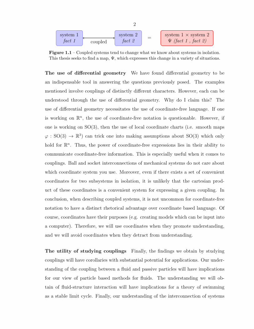
“What is the transformation?”. We depict this schematically in Figure 1.1
2
system 1fact 1
system 2fact 2coupled
=system 1 × system 2
Ψ (fact 1 , fact 2)
Figure 1.1 – Coupled systems tend to change what we know about systems in isolation.This thesis seeks to find a map, Ψ, which expresses this change in a variety of situations.
The use of differential geometry We have found differential geometry to be
an indispensable tool in answering the questions previously posed. The examples
mentioned involve couplings of distinctly different characters. However, each can be
understood through the use of differential geometry. Why do I claim this? The
use of differential geometry necessitates the use of coordinate-free language. If one
is working on Rn, the use of coordinate-free notation is questionable. However, if
one is working on SO(3), then the use of local coordinate charts (i.e. smooth maps
ϕ : SO(3) → R3) can trick one into making assumptions about SO(3) which only
hold for Rn. Thus, the power of coordinate-free expressions lies in their ability to
communicate coordinate-free information. This is especially useful when it comes to
couplings. Ball and socket interconnections of mechanical systems do not care about
which coordinate system you use. Moreover, even if there exists a set of convenient
coordinates for two subsystems in isolation, it is unlikely that the cartesian prod-
uct of these coordinates is a convenient system for expressing a given coupling. In
conclusion, when describing coupled systems, it is not uncommon for coordinate-free
notation to have a distinct rhetorical advantage over coordinate based language. Of
course, coordinates have their purposes (e.g. creating models which can be input into
a computer). Therefore, we will use coordinates when they promote understanding,
and we will avoid coordinates when they detract from understanding.
The utility of studying couplings Finally, the findings we obtain by studying
couplings will have corollaries with substantial potential for applications. Our under-
standing of the coupling between a fluid and passive particles will have implications
for our view of particle based methods for fluids. The understanding we will ob-
tain of fluid-structure interaction will have implications for a theory of swimming
as a stable limit cycle. Finally, our understanding of the interconnection of systems

3
through Dirac structures will allow us to relate the equations of motion of the discon-
nected system to equations of motion for the connected system, and thus may have
substantial benefits for modular modeling.
In the next three sections we will describe the main projects of this thesis.
1.1 A Fluid and its Particles
The first project of this dissertation seeks to a fluid flowing on a Riemannian manifold
M . For the sake of modeling, it is necessary to obtain a finite dimensional approxi-
mation to this system. Additionally, even the most fundamental expositions in fluid
dynamics view the system as a momentum equation on “volume elements” which (to
0th order approximation) may be represented as particles. Perhaps we can approxi-
mate the motion of the fluid using a finite set of particles. What are the obstacles to
doing this well? The most glaring obstacle is the fact that the fluid particles are all
coupled to each other, and so it is not clear how to ignore any of them. Moreover,
particle methods are usually developed by taking the Euler equations, which evolve
on Xdiv(M), and making approximations. However, the error analysis is fairly diffi-
cult because it is hard to describe the information lost during the approximation (see
Figure 1.2).
system on TDµ(M)
ut + u · ∇u = 0, on Xdiv(M)
particle method on TQN−body
compare?
error?
EP reduction
approximations
Figure 1.2 – A Signal Flow Diagram for the Error Analysis of Particle Methods?
However, we can start by choosing a good decomposition for the equations of
motion. In particular, we may view a fluid as evolving on the set of volume-preserving

4
diffeomorphisms, Dµ(M). By applying Lagrange-Poincare reduction with respect to
a carefully chosen symmetry group, we can write the equations of motion on the space
TQpart ⊕ E, where Qpart is the configuration manifold for a finite set of particle and
E is some infinite dimensional vector-bundle over Qpart. Armed with these equations
(which express the exact motion for the fluid) we can begin to surmise approximations
to the equations of motion (evolving on Qpart) which ignore the E component. These
approximations are equivalent to the creation of particle methods. However, unlike
particle methods such as SPH, these are derived by approximating the Lagrange-
Poincare equations on TQpart⊕E rather than the inviscid fluid equations on Xdiv(M).
We will find that this makes determining error bounds particularly simple (see Figure
1.3).
system on TDµ(M)
system on TQN−body ⊕ E
particle method on TQN−body
compare
error
LP reduction
closure method
Figure 1.3 – A Signal Flow Diagram for the Error Analysis of Particle Methods
There is much room for development in this perspective on finite dimensional
approximations of fluid motion. In particular, there are other symmetry groups which
we could reduce which result in particles that have shape and orientation and that
satisfy analogues of the circulation theorem. Additionally, there is no reason that the
main ideas developed could not be applied to any continuum system with particle
relabeling symmetry.

5
1.2 Swimming
When one watches a fish swim, something about it appears periodic. However it is not
really periodic because with each flap of the fins, the fish has changed locations and so
the state of the system has changed. In particular there is some translation and rota-
tion which relates the previous flapping of the fins to the current one. Therefore, the
motion is really only periodic modulo a (fixed) rotation and translation. Therefore,
the motion appears to be a relative closed orbit in phase-space. One would conjecture
that this motion is stable in some sense, which leads to the main conjecture of this
project:
Is swimming a relative limit cycle?
To begin thinking about this we first need to understand the system consisting of a
solid body immersed in a fluid as an unforced mechanical system. We let f ⊂ R3 be
a reference configuration, and we use the set
B := b : f → R3 | det([∂bi
∂xj]) = 1
as the set of configurations for the body. For each b ∈ B the state of the fluid may
be described by a vector field, u, on the set
eb := closure(R3\b(f)
).
Therefore, given a particular b ∈ B, the state of the system may be described by the
set
Ab := (b, u) ∈ TbB × X(eb) | b = u b on ∂f
and the phase space for the system can be given by the vector bundle over B given
by A = ∪b∈BAb. It is fairly simple to find a natural Lie bracket on sections of A, and
prove that A is a Lie algebroid. This allows us to use [Wei95] to derive the equations
of motion for a solid body in a fluid.

6
How can we use this to understand swimming as a relative limit cycle? First,
we must find a limit cycle in a reduced phase space. How do we do that? A quick
answer is provided by the averaging theorem. The averaging theorem suggests that
a sufficiently small periodic perturbation of a system on a Banach manifold with an
asymptotically stable point results in a system with a stable limit cycle. Therefore,
most of the work of this section will be directed towards proving the existence of an
asymptotically stable point in some reduced phase space, [A]. This would bring us
well on our way to interpreting swimming as a relative limit cycle.
stable submanifold ⊂ A
stable point ∈ [A]
swimming?
stable limit cycle ∈ [A]
periodic force
periodic force
reduction reduction
Figure 1.4 – A proposed understanding of swimming
Finding a stable point on [A] will require performing reduction by stages. The
first reduction is with respect to the particle relabeling symmetry and the second
reduction is with respect to frame-invariance (right-SE(3) symmetry). We will refer to
[CMR01] when we need equations of motion, and we will use [Wei95] when performing
SE(3) reduction. In any case, the left side of Figure 1.4 will be described in full.
Unfortunately, the process of adding a periodic force to get a stable limit cycle remains
at the conjecture level due to certain topological difficulties with infinite dimensional
spaces (they are not Banach). However, any finite dimensional model of a fluid which
is sufficiently well behaved (e.g. dissipates energy correctly) should exhibit these limit
cycles.
1.3 Interconnections as Dirac Structures
In the final chapter of this dissertation we will be using the following concept.
Definition 1.3.1. A linear Dirac structure D on a vector-space V is a dim(V ) di-

7
mensional subspace of V × V ∗ such that
〈β, v〉+ 〈α,w〉 = 0
for any (v, α), (w, β) ∈ D.
The generalization of Dirac structure to manifolds roughly consists of applying
this definition to each fiber of the tangeant bundle. In the last few decades Dirac
structures have emerged as generalization of symplectic and Poisson structures. In
particular, there is now a new formalism which one could call the Dirac formalism
formalism function structure eq. of motion
Lagrange L δ∫
(·)dt = 0 ddt∂L∂q− ∂L
∂q= 0
Hamilton H ·, · x = x,HDirac E D (x, dE(x)) ∈ D(x)
In summary, just as Poisson and symplectic structures can be used to derive dy-
namics from a Hamiltonian, so can a Dirac structure be used to derive dynamics
from an energy function. Additionally, one could take any power-conserving cou-
pling (e.g. soldering the wires of two circuits, or connecting an electrical system to
a mechanical one through an ideal motor). By the definition of Dirac structures,
the power-conserving coupling can be written as a Dirac structure. We call the
Dirac structures which express couplings “interaction Dirac structures.” However,
the observation that power-conserving interconnections could be expressed as Dirac
structures has not been used until recently. The question we seek to answer in this
final chapter is “how do we use interaction Dirac structures?”
More specifically, given mechanical systems with Dirac structures D1 and D2 on
manifolds M1 and M2, how do we use a interaction Dirac structure, Dint on M1×M2?
In order to answer this question, we will define a product, , and form the Dirac
structure
DC := (D1 ⊕D2) Dint,
which is a Dirac structure over M1×M2. We will find that DC is the Dirac structure

8
for the system which couples Dirac systems on Dirac manifolds (M1, D1) and (M2, D2)
using the power-conserving interconnection given by Dint.
Applications for this insight can be fairly broad. However, in this thesis we have
restricted our examples to the case of circuit-circuit interconnections and mechanical
interconnections by non-holonomic constraints.
1.4 Conclusion
We hope that this introduction has sufficiently whet the reader’s appetite. A fresh
graduate student looking for a new project to embark on should find ample material
here to start one. If there is a “moral” to this thesis, it is that much of the under-
standing known for isolated systems can carry over to coupled systems - it is just a
matter of working on the right spaces and resisting the urge to use coordinates. For
example, many couplings of Poisson systems result in Poisson systems. Ideal fluids
and rigid bodies in free space satisfy geodesic equations. We will find rigid bodies
immersed in ideal fluids satisfy geodesic equations as well. In conclusion, couplings
need not be so mysterious. Couplings may destroy desirable properties of subsystems,
but one should never lose hope. It is not uncommon for the beautiful aspects of the
subsystems to be reincarnated as new creatures in the coupled system. Working to
find these reincarnations can have significant benefits.
Reader’s Guide The chapters on particle methods and swimming require some
understanding of reduction by symmetry. A reader who is unfamiliar with the litera-
ture is encouraged to read chapter 2 and perhaps the first two chapters of [CMR01].
Chapters 3 through 5 are written such that they may be read in isolation from one
another. Therefore, the reader is generally encouraged to start with whichever project
most interests him or her.

9
Chapter 2
Background Material
In this section we provide some necessary background material in geometric me-
chanics, drawing primarily from [AM00] and [CMR01]. Two of the three projects
contained in this thesis are related to fluids. Such systems evolve on spaces which
are difficult to coordinatize. Therefore, there will be a bias in favor of geometrically
intrinsic expressions over coordinate based ones. We begin with a brief statement on
interpreting commutative diagrams in §2.1. In §2.2 we will describe how the Euler-
Lagrange equations can be written in a coordinate free notation upon choosing a
Covariant derivative for the tangent bundle. Additionally, there will be a heavy use
of Lie groups and geodesics on Lie groups (in particular, SE(3) and SDiff(M)). In
§2.3 we will review the nature of Riemannian geometry and Lagrangian mechanics on
Lie groups. Finally, as Lagrange-Poincare reduction is not thoroughly covered in most
classical mechanics courses, I will provide the minimal amount of concepts needed in
order to write down the Lagrange-Poincare equation in §2.4. This chapter is intended
as a reference and the reader is encouraged to skip the sections for which he or she
is already familiar with. The following material is not intended as an introduction
to geometric mechanics. An advanced undergraduate level introduction to geometric
mechanics is [Hol11a] and [Hol11b]. A slightly more advanced introduction is [MR99].
Finally, [AM00] is largely considered the “Bible” of the subject.
2.1 Reading Commutative Diagams
Let f : A → A′ and g : B → B′. Let Ψ : A → B and Ψ′ : A′ → B′. We say the
diagram in figure 2.1 commutes if g(Ψ(a)) = Ψ′(f(a) for any a ∈ A. Commutative

10
A A′
B B′
f
Ψ
g
Ψ′
Figure 2.1 – A commutative square
diagrams will make a few appearances in this thesis and they will generally convey
the message ‘Ψ acts on A like Ψ′ acts on A′’ or possibly ‘f acts on A like g acts
on B’. If g is the identity, so that B = B′, we get a commutative triangle (see
Figure 2.2) which says that f will send elements of the equivalence classes Ψ−1(b)
A A′
B
f
Ψ Ψ′
Figure 2.2 – A commutative triangle
to (Ψ′)−1(b). In summary, these diagrams convey the message that some kind of
structure is preserved. For a gentle introduction to this perspective see [LS09], or for
a more advanced introduction see [Mac00].
2.2 Lagrangian Mechanics
Given a Lagrangian, L : TQ → R, on an n-dimensional configuration manifold Q,
we can express the Euler-Lagrange equations in local coordinate (q1, . . . , qn) by the
expression:d
dt
∂L
∂qi− ∂L
∂qi= 0.
Implicitly we are using the Euclidean inner product on Rn to write the equations
of motion locally. If we desire a geometrically intrinsic expression for the Euler-
Lagrange equation, we need to replace ddt
with a covariant derivative and provide
intrinsic notions to replace the partial derivatives ∂L∂qi
and ∂L∂qi
. All of these issues are

11
solved by choosing a covariant derivative. For a general Q there is no canonical way
of making this choice. In the case that Q is a Riemannian manifold, however, there is.
In this section we will provide the necessary ingredients from Riemannian geometry
to write down a geometrically intrinsic expression for the Euler-Lagrange equation.
We begin by defining a connection.
Definition 2.2.1 (Connection). Let Q be a manifold. A connection is a mapping
∇ : X(Q)× X(Q)→ X(G) such that:
1. ∇X(Y + Z) = ∇X(Y ) +∇X(Z).
2. ∇X(fY ) = X[f ]Y + f · ∇X(Y ).
3. ∇X+Y (Z) = ∇X(Z) +∇Y (Z).
One can understand a connection as a way of differentiating vector fields. It is
worth noting that the first argument of a connection need not be a vector field, but
may be a single vector v ∈ TQ, while the second item need only be a vector field along
a path qε ∈ Q tangent to v. Therefore, using ∇ we can define a covariant derivative.
Definition 2.2.2 (Covariant Derivative, Geodesic). Given a path q(t) ∈ Q and a
vector field v(t) ∈ Tq(t)Q above q(t) we can define the covariant derivative
Dv
Dt:= ∇q(v).
Additionally, the path q(t) is called a geodesic if
Dq
Dt:= 0,
where we define q = dqdt
. Lastly, the covariant derivative acts on covector fields above
q by the formula
〈DαDt
, v〉 = 〈α, DvDt〉 − d
dt〈α, v〉.

12
Given a Lagrangian L : TQ → R we can define the Legendre transform ∂L∂q
:
TQ→ T ∗Q by
〈∂L∂q
(q, v), δq〉 :=d
dε
∣∣∣∣ε=0
(l(q, v + εδq)) .
It is notable that if q(t) is a curve in Q, then both ∂L∂q
(q, q)(t) and DDt
(∂L∂q
)are covector
fields above q(t). Finally we define the partial derivative ∂L∂q
by:
〈∂L∂q
(q, v), δq〉 :=d
dε
∣∣∣∣ε=0
(l(qε, vε))
for an arbitrary curve (qε, vε) ∈ TQ such that ddε
∣∣ε=0
qε = δε and DvεDε
= 0.
The Euler-Lagrange equations are given by
D
Dt
(∂L
∂q
)− ∂L
∂q= 0.
We can stop here, but we have not addressed the issue of how one chooses a connec-
tion. In general, one should simply do what is easiest for the circumstances at hand.
However, if Q is a Riemannian manifold there is a “natural” choice [AM00, §2.7].
Theorem 2.2.1 (The Fundamental Theorem of Riemannian Geometry). If Q is a
Riemannian manifold with metric ,, then there exists a unique connection, ∇,
on Q such that
∇XY −∇YX = [X, Y ]
and
X[ Y, Z ] = ∇XY, Z + Y,∇XZ
we call ∇ the Levi-Cevita connection.
The Levi-Cevita connection is given implicitly by Koszul’s formula,
2 ∇XY, Z =X[ Y, Z ] + Y [ X,Z ]− Z[ Y,X ]
+ [X, Y ], Z − [X,Z], Y − [Y, Z], X .

13
In particular, if L(q, q) = 12 q, q then the Euler-Lagrange equations become
D
Dt
(∂L
∂q
)= 0,
and are equivalent to the geodesic equations on Q with respect to the metric field,
, [AM00, §3.7].
2.3 Lagrangian Mechanics on Lie Groups
In this section we will review the geometry and Lagrangian mechanics of Lie groups.
In particular we will pay attention to the case of Riemannian metrics which are
invariant with respect to group translations.
Definition 2.3.1 (Group). A group, (G, ), is a pair which consists of a set G and
a composition : G×G→ G which satisfies the following properties:
1. The composition is associative (i.e., g (h k) = (g h) k ).
2. There exists an identity element, e ∈ G, defined by the condition e g = g for
every g ∈ G.
3. For each g ∈ G there exists an inverse g−1 defined by the condition g−1 g = e.
If G is a manifold, and , and g 7→ g−1 are smooth, then G is called a Lie Group.
The examples of Lie groups most useful for this thesis are the special Euclidean
group, SE(3), and the special diffeomorphism group, Dµ(M), for a volume manifold.1
In addition to the concept of a Lie Group we will also use its infinitesimal coun-
terpart, the Lie Algebra.
Definition 2.3.2 (Lie algebra). A Lie algebra is a pair g, [, ] consisting of a vector
space g and a bracket [, ] : g× g→ g which satisfies the following properties:
1. The bracket satisfies the Jacobi identity, [a, [b, c]]− [b, [a, c]] + [c, [a, b]] = 0.
1This latter group is actually an infinite dimensional Lie group. The consequences of this are notinvestigated in this dissertation. For more information see [BK09].

14
2. The bracket is anti-symmetric, [a, b] = 0.
In particular, the Lie group, G, with identity, e, is equipped with a Lie algebra,
g = TeG. The Lie bracket is induced by the commutator of vector fields [AMR09,
Chapter 5].
Deriving Lie brackets on Lie groups . Given a Lie group, G, with identity, e,
one can use the following procedure to derive the bracket on the Lie algebra, g = TeG.
1. For each g ∈ G define the AD-map or inner automorphism ADg : G → G by
Ig(h) = ghg−1.
2. Define the Ad-map2, Adg = Te AD, which can be written as Adg(η) ≈ g ·η · g−1.
3. For each ξ ∈ g define the ad-map3 adξ = ddt
∣∣t=0
Adg for a curve g(t) with
ξ = dgdt
∣∣t=0
. This defines the Lie bracket [ξ, η] := adξ η.
Jacobi’s identity follows from interpreting elements of g as left invariant vector
fields on G. Noting that left invariant vector fields form a Lie subalgebra of the set
of all vector fields on G allows us to carry the Lie bracket on X(G) to g [AMR09,
Chapter 5].
Invariant metrics and Euler-Poincare reduction . Let G be a Lie group with
identity, e, and a left invariant metric, ,. Left invariance means
v, w = g · v, g · w
for any (v, w) ∈ TG⊕TG and g ∈ G. Equivalently, we can choose an inner product
,e on the Lie algebra g := TeG and construct the left invariant metic v, w :=
λtriv(v), λtriv(w) e using the left-trivializing diffeomorphism λtriv(g, v) = Tg−1 · v
which takes TG→ g.
2Also called the “adjoint map”3Called the “adjoint map” as well

15
If we define a Lagrangian, L(g, g) = 12 g, g , then the previous section tells
us that the Euler-Lagrange equations are given by
D
Dt
(g[)
= 0
where g[ is a curve in T ∗G given by the contraction of g(t) ∈ TG with the metric
tensor. We may write g(t) = g(t) ·ξ(t) for some curve ξ(t) ∈ g := TeG. From Koszul’s
formula one can observe that left invariance of , implies left invariance of the
covariant derivative, so that
T ∗g · DDt
(g[)
=D
Dt
(g∗g[
).
Let η be an arbitrary element of g and note that T ∗g · ξ[ = g[. Then we find along a
curve g(t) which satisfies the Euler-Lagrange equations
0 = 〈Dg[
Dt, Tg · η〉
= 〈T ∗g−1 · DDt
(ξ[), T g · η〉
= 〈∇ξ(ξ[), η〉
=d
dt ξ[, η −〈ξ[,∇ξη〉
= 〈dξ[
dt, η〉 − 1
2〈ξ[, [ξ, η]− (ad∗ξ η
[)] − (ad∗η ξ[)]〉.
We can simplify this further using the identities
〈ξ[, [ξ, η]〉 = 〈ad∗ξ ξ[, η〉
〈ξ[, (ad∗ξ η[)]〉 = 〈ad∗ξ η
[, ξ〉 = 〈η[, adξ ξ〉 = 0
〈ξ[, (ad∗η ξ[)]〉 = 〈ad∗η ξ
[, ξ〉 = 〈ξ[, [η, ξ]〉 = −〈ad∗ξ ξ[, η〉
which imply
0 = 〈dξ[
dt− ad∗ξ ξ
[, η〉.

16
Letting η vary over all g implies the Euler-Poincare equation:
dξ[
dt= ad∗ξ ξ
[.
(see [MR99, Chap. 13] for matrix Lie groups).
Example 2.3.1 (Rigid Body on SO(3)). Consider the Lie Group SO(3). We can
equate the Lie algebra with R3 through a map ∨. Then, both the adjoint action and
coadjoint action are represented by the cross product. The Euler-Lagrange equations
for the Lagrangian
L(R, R) =1
2
(∨(R−1R)T · I · ∨(R−1R)
)therefore reduce to the Euler-Poincare equation
Π = Π× Ω
where Π = I · Ω.
Finally, we could have considered a right invariant metric. That is to say, a metric
which satisfies the invariance property
vg, wg = v, w , ∀g ∈ G.
This would result in the (right) Euler-Poincare equation
dξ[
dt= − ad∗ξ ξ
[.
Example 2.3.2 (Ideal Fluids, [Arn66]). Let M be a Riemannian manifold and con-
sider the Lie Group, SDiff(M), consisting of the volume-preserving diffeomorphisms
of M . The Lagrangian, L : T SDiff(M)→ R, given by
L(ϕ, ϕ) :=1
2
∫M
‖ϕ(x)‖2dx

17
is right SDiff(M) invariant. The resulting (right) Euler-Poincare equations occur on
the Lie algebra of SDiff(M), which is identified with the set of divergence-free vector
fields, Xdiv(M), equipped with the Lie bracket given by the commutator of vector fields.
The resulting Euler-Poincare equations are the inviscid fluid equations ut+∇uu = ∇p.
On Rn this takes the more familiar form ut + u · ∇u = ∇p. See [AK92, Chapter 1]
for details on the Hamiltonian perspective.
2.4 Lagrange-Poincare Equations
In this section we state the (right) Lagrange-Poincare equations. The material of this
section is taken from [CMR01]. Let π : Q→ [Q] be a principal bundle with structure
group G induced by a right action. Given a q ∈ Q we use the notation [q] := π(q) to
denote the orbit given by q ·G. Additionally there exists a lifted action on TQ through
the tangent lift of the action of G. We denote the action of g ∈ G on q ∈ Q by qg
and on v ∈ TQ by vg. We denote the equivalence class of a v ∈ TQ by [v] = v · G.
The collection of these equivalence classes is denoted by [TQ]. Given a Lagrangian
on TQ which is right invariant with respect to the action of G there must exist a
well-defined Lagrangian on [TQ] given by l([q, v]) = L(q, v). One would expect the
Euler-Lagrange equations to have the same symmetry, since they are determined by
the Lagrangian. Such a symmetry would induce consistent dynamics on [TQ]. To
find these equations we must first understand how variations of curves in Q will lead
to variation of curves in [TQ]. Unfortunately, the quotient [TQ] is a fairly abstract
space to consider writing equations of motion on. More concrete formulations of the
equations can be found on the bundle T [Q]⊕ g (to be defined), which is isomophic to
[TQ]. In this section we will produce an isomorphism from [TQ] to T [Q] ⊕ g where
we will also be able to state the reduced equations of motion using suitably chosen
covariant derivatives. We start by defining the adjoint bundle, g.
Definition 2.4.1 (Adjoint Bundle). Given the action of G on Q we may define an
action on Q × g by (q, ξ) 7→ (qg,Ad−1g (ξ)). The adjoint bundle is the vector bundle

18
π : g→ [Q] where
g :=Q× g
G,
and π([q, ξ]) = [q]. This bundle is also equipped with a fiber-wise Lie bracket given by
[[q, ξ], [q, η]] = [q, [ξ, η]] .
Definition 2.4.2 (Principal Connection). A principal connection is a mapping A :
TQ→ g which satisfies
1. For any ξ ∈ g, A(ξQ(g)) = ξ where ξQ is the infinitesimal generator of ξ.
2. A(vg) = Ad−1g ·A(v) for any v ∈ TQ, g ∈ G.
The definition of principal connection provided here is designed to handle symme-
tries with respect to right group action (see [CMR01] for the case of left actions). In
particular, principal connections serve as morphisms which carry the action on TQ
to the Ad-map on g. That is to say, A is designed to make the following diagram
commute.
TQ TQ TQ
g g g
g
A A
g
h
A
h
gh
gh
where we are using the right action on Q in the top row of the diagram and the right
adjoint action, Ad−1g , on g in the bottom row.
We define the horizontal distribution to be the constraint distribution H :=
kernel(A) ⊂ TQ. Additionally, the vertical distribution is defined as
V := ξQ(q) ∈ TQ : q ∈ Q, ξ ∈ g.
The distributions satisfy the following properties:

19
• The horizontal distribution is G invariant. That is to say, H ·G ⊂ H.
• The horizontal distribution is complementary to the vertical distribution. That
is to say, H ∩ V is the 0 section of TQ, and H⊕ V = TQ.
• The vertical distribution is integrable. This is because the infinitesimal gener-
ators satisfy [ξQ, ηQ] = [ξ, η]Q.
Since H and V are complementary distributions, we may define projection onto the
horizontal and vertical distributions, denoted by hor : TQ → H and ver : TQ → V,
respectively. Additionally, given a x ∈ T [Q] and a q ∈ π−1(x), there is a unique
vector x↑q ∈ TqQ such that x↑q ∈ H and Tπ(x↑q) = x. We call the mapping, x 7→ x↑q
the horizontal lift of x above q . One may hope that H is integrable. However, this
is generally not the case. A measurement of the integrability of H is given by the
curvature tensor.
Definition 2.4.3 (Curvature Tensor). The curvature tensor of a principal connection
A : TQ→ g is the g valued two form on Q given by the expression
B(q, δq) = dA(hor(q), hor(δq)).
Additionally, the reduced curvature tensor is g valued two form on [Q] given by
B(x, δx) = [q, B(x↑q, δx↑q)].
The choice of a principal connection induces a bundle map from A : TQ → g
given by A(q, v) = [q, A(q, v)]. This makes ΨA := Tπ ⊕ A [τQ] : [TQ] → T [Q] ⊕ g
into an isomorphism. A principal connection, A, also induces a covariant derivative
on g, given byD
Dt([q(t), ξ(t)]) = [q(t), [ξ, A(q)] + ξ]
for a curve [q(t), ξ(t)] ∈ g. The covariant derivative on g induces a covariant derivative

20
on the dual bundle g∗, defined by the condition
〈 DDt
[q(t), α(t)], [q(t), ξ(t)]〉 =d
dt〈α(t), ξ(t)〉 − 〈 D
Dt[q(t), ξ(t)], [q(t), α(t)]〉
for a curve [q(t), α(t), v(t)] ∈ g∗⊕ g. These notions are enough to state the Lagrange-
Poincare reduction theorem [CMR01, Theorem 3.4.1].
Theorem 2.4.1 (Lagrange-Poincare Reduction Theorem). Let π : Q → [Q] be a
principal bundle with structure group G. Let L : TQ→ R be a Lagrangian with right
G-symmetry. Finally, let there exist a covariant derivative on [Q]. Then given a
curve q(t) ∈ Q, the following are equivalent:
1. q(t) satisfies the Euler-Lagrange equations for L.
2. q(t) extremizes the action∫L(q, q)dt with respect to variations with fixed end-
points.
3. For x(t) = π(q(t)) ∈ [Q], ξ(t) = [q(t), A(q(t), q(t))] ∈ g and l = L ΨA :
T [Q]⊕ g→ R the Lagrange-Poincare equations
D
Dt
(∂l
∂x
)− ∂l
∂x= 〈 ∂l
∂ξ, ix · B〉 on T [Q]
D
Dt
(∂l
∂ξ
)= − ad∗
ξ
(∂l
∂ξ
)on g.
4. (x, ξ)(t) = (π(q(t)), [q(t), A((q, (q))(t)) ∈ T [Q]⊕g extremizes the action∫l(x, x, ξ)dt
with respect to variations (δx, δξ) ∈ T [Q]⊕ g where δx is a variation of x with
fixed endpoints and δξ = DηDt− [ξ, η] +B(δx, x).
The derivatives ∂l∂ξ
and ∂l∂x
can be viewed as fiber derivatives, while the derivative
∂l∂x
should be viewed as induced by the covariant derivative on [Q] as in §2.2
Example 2.4.1 (The Kaluza-Klein Formalism for Charged Particles). Consider an
electron moving in R3. Let the configuration space be Q = R3 × S1. Consider the
Lagrangian
L(q, q, θ, θ) =1
2m‖q‖2 +
1
2‖ω1(q) · q + θ‖2.

21
We observe that L has S1 symmetry, as it does not depend on θ. The quotient space
is [Q] = R3 and we choose the principal connection
A(q, q, θ, θ) = θ,
where we interpret θ as a vector above θ = 0 on the right-hand side. The curvature
of A is given by B = dω. We observe that the horizontal equations are
mx = ixdω
while the vertical equations are simply θ(t) = θ(0). Equating R∗ with R through
the standard Euclidean metric induces the Hodge star, which sends dx ∧ dy 7→ dz,
dz∧dx 7→ dy, and dy∧dz 7→ dx. Upon setting dω = e(B1dy∧dz+B2dz∧dx+B3dy 7→
dz) we find that the horizontal equations become mx = ex× B. This is the standard
Lorentz force law for charged particles.

22
Chapter 3
Geometric Foundations forParticle Methods
There are two major competing representations for the state of a fluid, Eulerian
and Lagrangian (alternatively described as the spatial description and the material
description). In the Lagrangian description, the fluid is represented by a volume-
preserving diffeomorphism. This diffeomorphism evolves with time and stores the
data of where fluid particles go. In contrast, the Eulerian description of fluids only
keeps track of the velocity field from the reference frame of the observer, and thus par-
ticle locations are forgotten. In this chapter we will be concerned with understanding
numerical methods for fluids which adopt the Lagrangian description.
Figure 3.1 – How a volume-preserving diffeomorphism represents the state of a fluid
A Lagrangian method of particular concern is a particle method which represents
the corresponding diffeomorphism by the motion of a finite number of particles1. Un-
like Eulerian methods, such as fixed-grid finite-difference, it is not entirely clear how
to estimate or even write down error bounds for particle methods over infinitesimal
times. In the case of Eulerian methods with fixed grids, the accuracy is controlled
1This excludes meshless methods such as the Vortex Method.

23
by the grid spacing, which is decoupled from time. This separation of space and
time allows for the error analysis of most Eulerian schemes. However in the case of
particle methods, the analogue of grid spacing is particle spacing, and the spacing
of the particles is not static but governed by the dynamics of the chosen method.
Due to the time-dependence of the particle spacing, discovering error bounds for par-
ticle methods is particularly difficult. Upon encountering this problem, it becomes
desirable to find a way to move particles around to regulate particle spacing. How-
ever, this presents one with another problem. Upon moving the particles around to a
preferable arrangement, how does one choose the velocities? More specifically, given
a method for estimating vector-fields from particle positions and velocities, how does
one rearrange the particles and choose the velocities in such a way that the estimate
is unaltered? The key to answering this is to tie everything to a reconstruction map-
ping, a method which estimates the fluid velocity field given particle positions and
velocities.
R
Figure 3.2 – Schematic of a Reconstruction Map
In particular, this chapter will demonstrate the following claims:
Claim 3.0.1. Each reconstruction mapping induces a corresponding particle method.
Claim 3.0.2. Certain reconstruction mappings provide a means of moving the parti-
cles manually and choosing velocities so as to leave the estimated velocity field unal-
tered.
Claim 3.0.3. Claim 3.0.1 and Claim 3.0.2 can be combined to create particle methods
with error bounds.

24
Additionally, we will attempt to analyze the smoothed particle method (SPM).
However, the correspondence between reconstruction mappings and particle methods
is many-to-one. Therefore we are faced with an arbitrary choice when trying to find
a reconstruction mapping corresponding to SPM.
Warning! One would naturally expect a chapter on numerical methods to include
computational experiments. In order to avoid creating unmet expectations, let me
warn the reader now that this will not be done in this chapter. Indeed, we will be
proposing a new framework for making new numerical methods and analyzing them.
However, the task of getting an appropriate configuration manifold for error analysis
of particle methods is a substantial one. Clearly computation is the next step in this
project, and some ideas are presented in the final section.
Problem formulation Let (M,,) be a Riemannian manifold filled with an
inviscid fluid. It is not difficult to imagine that the state of an incompressible fluid
may be represented by a volume-preserving diffeomorphism (see Figure 3.1).
It was proven by V. I. Arnold that the inviscid fluid equations can be derived from
the Lagrangian
L(ϕ, ϕ) =1
2
∫M
‖ϕ(x)‖dx
on the set of volume-preserving diffeomorphisms of M , denoted as Dµ(M). This was
done through a symplectic reduction with respect to the particle relabeling symme-
try of the system. The reduction yielded the traditional Euler equations for an ideal
fluid on the vector space of divergence-free vector fields over M , denoted Xdiv(M)
[Arn66, AK92]. However, we may reduce by other symmetries instead. In particular,
if we let Qpart be the configuration manifold for n non-overlapping point particles
embedded in M , then there exists a vector bundle, πE : E → Qpart, as well as a
symmetry reduction procedure which places the equations of motions on the vector
bundle TQpart⊕E. The significance of being able to write the equations of motion on
TQpart⊕E is that TQpart is a submanifold. Therefore, given a particle method (which
is an ordinary differential equation on TQpart) we may compare it with the exact equa-

25
tions of motion. In particular, the reduction procedure is that of Lagrange-Poincare
reduction as demonstrated in [CMR01] (see also Section §2.4) and our perspective on
error is communicated by the cartoon signal flow diagram in Figure 3.3.
system on TDµ(M)
system on TQpart ⊕ E
particle method on TQpart
compare
error
LP reduction
closure method
Figure 3.3 – A signal flow diagram for the error analysis of particle methods
The primary task of this paper is to specialize the equations and geometric con-
cepts of [CMR01] to the case of reduction by a certain Lie-subgroup, G ⊂ Dµ(M).
Previous work There are a number of preexisting mesh-free methods which have
been applied to fluids. Motivations for the development of such methods include:
• They avoid complex mesh generation techniques.
• There is no mesh entanglement.
• They can handle odd-shaped and/or time-dependent domains with relative ease.
• They are easy to modify for use in multi-physics simulations.
We are interested in the class of methods known as “particle methods” which store the
data of the fluid on a finite number of moving particles. The most well-established
particle method today, smooth particle hydrodynamics (SPH), was introduced in
[GM77] and [Luc77] for the purpose of astrophysical simulations. It was realized that
the basic idea of SPH could be generalized to deal with a variety of partial differential
equations (PDEs) including fluids [GM82]. However, SPH was found to have a number

26
of problems (e.g., consistency, boundary conditions, stability), which then motivated
the search for improvements and new methods. Most notably, the reproducing kernel
particle method (RKPM) was developed to address the inaccuracy of SPH on the
boundary of the domain [LJZ95, GL98]. Since then, a number of improvements have
been made to SPH, and a variety of other methods have appeared on the scene. Finite-
point methods approximate functions involved in a PDE through a set of moving
collocation points [OIT96, OIZ+96]. Local Petrov-Galerkin schemes use the “local
weak form” of the PDE in question via a moving set of basis functions [AS02]. A
thorough survey of mesh-free methods (including a few not mentioned here) can be
found in [Liu03]. All of these methods are designed to carry the velocity field data
by storing it, at least implicitly, on a finite number of nodes. This is distinct from
both Chorin’s vortex method and vortex blob method, where each “particle” stores
vorticity data (although a velocity field is implied by the vorticity equation) [Cho73].
In this chapter we will form geometric foundations for the creation and error anal-
ysis of methods in the spirit of SPH, where the particles carry velocity information.
In particular we will be using much work from the field of geometric mechanics and
Lie group theory. The analysis of mechanical systems on Lie groups traces back to
the time of Poincare, and the corresponding brackets are closely related to the results
of Arnold, Kirillov, Kostant, and Souriau in the 1960s [MR99, chapter 10]. In partic-
ular, Arnold discovered that the Euler fluid equations are Euler-Poincare equations
corresponding to the geodesic equations on the group of special diffeomorphisms of a
manifold [Arn66]. This result was then leveraged to prove local existence in time of
the Euler equations by using Sobolev norms [EM70]. Simultaneously, an understand-
ing of more general forms of reduction by symmetry were desired, and symplectic
reduction by the action of a Lie group on a symplectic manifold was articulated in
[MW74]. Since then, it has been observed repeatedly that a number of systems ap-
pear to be symmetry reduced systems by non-transitive group actions. In particular,
a number of systems in particle physics and gauge theory had this structure (see
[Ble81] and references therein). In order to understand the resulting quotient space
of reduction by non transitive group actions a principal connection is chosen which

27
places the dynamics on a vector bundle (dubbed a “Lagrange-Poincare bundle”).
This process is called Lagrange-Poincare reduction [CMR01]. Lagrange-Poincare re-
duction was explicitly used in [Kel98] and [KM00] to understand the locomotion of
a vehicle in potential flow. It can be argued that Lagrange-Poincare reduction was
implicitly understood in the analysis of swimming at low Reynolds numbers [SW89],
even though this work was decades before Lagrange-Poincare reduction took on the
form found in [CMR01].
Outline In §3.1 we seek to translate [CMR01] to the case of (right) subgroup re-
duction. That is to say, we hope to reduce a system on a Lie group G by some
subgroup Gs ⊂ G equipped with the action of right translation. We will not re-
view Langrage-Poincare reduction in full, but only translate the concepts necessary
to write down the Lagrange-Poincare equations. These necessary concepts are: the
quotient bundle, the adjoint bundle, the principal connection, the curvature tensor,
and the covariant derivatives. We then apply these constructions to fluids in §3.2 for
the case of reduction by the isotropy subgroup of a finite set of points, G ⊂ Dµ(M).
We will find that the quotient manifold is isomorphic to the configuration manifold
for point particles, Qpart, and the adjoint bundle is isomorphic to the vector bun-
dle of vector fields which vanish at n-points, πE : E → Qpart. These identities put
the Lagrange-Poincare equations on the space TQpart ⊕ E. In §3.4 we use a closure
method which effectively “ignores the vertical equation”. Additionally, a higher-order
closure method is proposed which provides an extra order of accuracy in time, while
sacrificing geometric properties in the process. This yields an ODE on TQpart which
we interpret as a particle method. We will find that smoothed particle methods fit
under this construction (modulo time reparametrization), but we will not be able to
perform error analysis on them. Additionally, we will find that under certain circum-
stances it is possible to re-arrange particles, and thus to bound the spacing between
the particles. Enforcing this bound would open the door for error analysis of a new
class of particle methods. In §3.5 we concoct a numerical method where error analysis
is possible. We find the proposed method to be accurate to second order in space (via

28
the bound enforced on particle spacing) and second or third order in time, depending
on the closure method.
3.1 Subgroup Reduction
In this section we review Lagrange-Poincare reduction in the context of reduction by
subgroups. For brevity we state all claims and theorems while referring to [CMR01]
for proofs2.
Let G be a Lie-group and Gs ⊂ G a Lie-subgroup. We equip Gs with the action
defined by right translation on G. That is to gs ∈ Gs acts on G by gs : g ∈ G 7→
ggs ∈ G for each gs ∈ Gs. Let gs denote the Lie algebra of Gs. The infinitesimal
generator of ξs ∈ gs is the vector field on G given by the map g ∈ G 7→ g · ξ ∈ TgG.
If Gs acts on a manifold X we may define the equivalence relation
x1 ∼Gs x2 ⇐⇒ ∃gs ∈ Gs such that x1 = x2 · gs
for x1, x2 ∈ X. Throughout this paper we will denote the equivalence class of x ∈ X
under a right Gs action by [x]s and the set of equivalence classes by XGs
. For this
section we define [G] = GGs
the set of equivalence classes with the quotient projection
π : g ∈ G 7→ [g]s ∈ [G].
Because Lie groups act freely and properly on themselves, their subgroups do as
well. This ensures that π : G → [G] is a principal bundle (see Proposition 4.2.23 in
[AM00], see also [Ebi70] for technicalities related to infinite dimensional Lie groups).
Additionally, Gs is equipped with a right action on TG given by tangent lift of the
2In this paper we will be concerned with reduction by right group actions. The paper [CMR01]is concerned with left group actions. However, all the content remains intact upon substituting leftactions with right actions, Adg with Ad−1
gs and adξ with − adξs .
29
action on G. That is to say
gs : v ∈ TgG 7→d
dε
∣∣∣∣ε=0
(gε · gs) ∈ Tg·gsG,∀gs ∈ Gs
where v = dgεdε
∣∣ε=0
. We may denote the quotient projection τ : TG → [TG] := TGGs
.
One should note that Tπ 6= τ and T [G] 6= [TG]. These quotient bundles relate to
Lagrangian mechanics for the following reason: If the Lagrangian, L : TG → R,
possesses right Gs-invariance then there exists a reduced Lagrangian l : [TG] → R
defined by the condition l τ = L. One could hypothetically compute dynamics on
[TG]. However, [TG] is not a tangent bundle but a Lie-algebroid, and we can not
resort to traditional Lagrangian mechanics3. To write the dynamics in a familiar
form it is useful to find an isomorphism to the bundle T [G] ⊕ gs where gs is the
adjoint bundle (§2.4) and T [G] is the tangent bundle of [G]. There are many such
isomorphisms, but one of particular interest is an isomorphism induced by a principal
connection (§3.1).
Principal connections for subgroups The infinitesimal action of Gs on G will
not produce the entire tangent bundle, TG, but only a sub-bundle, Vs, known as the
vertical bundle. The choice of a principal connection allows one to split any vector
in TG into a part produced by infinitesimal actions of Gs and a part which is not.
We may refer to [CMR01] for proofs with left group actions. In this paper we are
concerned with right group actions which yield a slightly different set of conventions
(see for example [MMO+07] or [Ble81]). For the case of subgroups, Definition 2.4.2 for
principal connections can be written in more specific terms. A principal connection
for a subgroup Gs ⊂ G equipped with right action on G is a gs-valued one-form
A ∈∧1(G, gs) such that
A(v · gs) = Ad−1gs A(v) (3.1)
A(Tg · ξs) = ξs (3.2)
3this non-traditional type of mechanics is found in [Wei95, Mar01]

30
where v ∈ TG, ξs ∈ gs. Similarly the horizontal and vertical distributions take a
specific form in the case of subgroups.
Definition 3.1.1 (Vertical and Horizontal Distributions for subgroups). We define
the vertical distribution
Vs := g · ξs : ξs ∈ gs, g ∈ G.
Additionally, a horizontal distribution is any distribution, H, such that H⊕Vs = TG.
We say that H is Gs invariant if H ·Gs ⊂ H.
Proposition 3.1.1. Given a Gs invariant horizontal distribution, H, there exists a
unique principal connection A ∈∧1(G, gs) such that kernel(A) ≡ H. Conversely, a
principal connection, A ∈∧1(G, gs), induces a Gs-invariant horizontal distribution
H = kernel(A).
As Vs is the kernel of Tπ we find that Tπ restricted to H is an isomorphism
between the fiber Hg ⊂ TgG and the fiber T[g][G]. Therefore, given x ∈ [G] and
g ∈ π−1(x), there exists a mapping called the horizontal lift which takes a vector
x ∈ Tx[G] to the unique vector x↑g ∈ Hg, such that Tπ(x↑g) = x. Additionally, one can
take a curve x(t) ∈ [G], set x = dxdt
, and solve the ODE on G given by:
g(t) = x↑g(t)(t)
for some initial condition g ∈ π−1(x(0)). The solution curve, denoted x↑g(t) ∈ G, is
called the horizontal lift of the curve x(t) ∈ [G].
Proposition 3.1.2. Given a principal connection, A : TG → gs, the induced hori-
zontal lift satisfies
x↑g · gs = x↑g·gs
for any vector x ∈ T [G], g ∈ π−1(x), gs ∈ Gs. Moreover, for any curve x(t) ∈ [G] we
have:
x↑g0(t) · gs = x↑g0·gs(t).
31
Since H ⊕ Vs = TG is a direct sum, there exist projections ver : TG → Vs and
hor : TG→ H such that v = hor(v) + ver(v) for any v ∈ TG. This allows us to state
the following corollary to 3.1.2:
Corollary 3.1.1. Given a principal connection A : TG→ gs the Lie bracket of vector
fields satisfies
[ver(X), hor(Y )] = 0
for any vector fields X, Y ∈ X(G).
We conclude this section with some thoughts on how infinitesimal loops in T [G]
should be expressed by a principal connection. Note that Vs is integrable by the
Frobenius theorem. However, the horizontal distribution, H = kernel(A), may not
be. The curvature tensor (to be defined) is a gs-valued two-form which measures the
non-integrability of H.
Moreover, the curvature tensor can also be written more specifically in the case
of subgroup reduction. Given A : TG→ gs, we define dA to be the unique gs-valued
two-form such that
〈µ, dA〉 = d〈µ,A〉
for an arbitrary µ ∈ g∗s. The curvature tensor of A is the gs valued two-form defined
by
B(v, w) = dA(v, w) + [A(v), A(w)].
From this, it may not be entirely clear how B measures non-integrability. The fol-
lowing proposition addresses this.
Proposition 3.1.3. Given vector-fields X, Y ∈ X(G) we have the identity
B(X, Y ) = A([hor(X), hor(Y )])
where [, ] is the Lie-bracket on vector-fields.
As a result, H is integrable if and only if B = 0.

32
3.2 Subgroup Reduction for Fluids
In the previous section we assembled the necessary constructions for subgroup reduc-
tion. In this section we then specialize this construction to the case of fluids. Again,
Dµ(M) is the infinite-dimensional Lie group of volume-preserving diffeomorphisms of
a Riemannian manifold (M,,). Let 1, . . . ,n ∈ M be a set of points. We use
the shorthand = (1, . . . ,n) and F () = (F (1), . . . , F (n)) for any map F
with domain M . We can then define the isotropy subgroup,
G := ϕ ∈ Dµ(M) : ϕ() = .
We will denote an arbitrary element of G by g and an arbitrary element of Dµ(M)
by ϕ. It is simple to observe that G is a Lie subgroup of Dµ(M). The Lie algebra
of G is the Lie subalgebra g ⊂ Xdiv(M) consisting of divergence-free vector fields
ξ on M such that ξ() = 0 (see Figure 3.4 ). Additionally, note that a tangent
vector in TϕDµ(M) is a mapping δϕ : m ∈ M 7→ δϕ(m) ∈ Tϕ(m)M . This allows
us to understand the infinitesimal generator of ξ ∈ g on Dµ(M) as the mapping
ϕ 7→ Tϕ · ξ, where we view ξ as mapping from m ∈M → TmM and Tϕ as a mapping
TmM → Tϕ(m)M .
Figure 3.4 – The vector field represents an element of g where is given by the reddot.
The goal of this section will be to perform LP-reduction on TDµ(M) by the
symmetry group G. As in the previous section, we equip G with the right action
on Dµ(M) and set [Dµ(M)] := Dµ(M)
Gwith projection π : Dµ(M)→ [Dµ(M)].
33
Proposition 3.2.1. Let Qpart be the configuration manifold for n non-overlapping
particles. That is to say,
Qpart = (m1, . . . ,mn) ∈M × · · · ×M : i 6= j =⇒ mi 6= mj.
Then [Dµ(M)] ≡ Qpart.
Proof. Define the set-valued map Ψ : Qpart → ℘(Dµ(M)),
Ψ(m1, . . . ,mn) := ϕ ∈ Dµ(M) : ϕ() = (m1, . . . ,mn).
We first prove that Ψ maps to co-sets. Take an arbitrary g ∈ G. Then we find
Ψ(m1, . . . ,mn) · g = ϕ g : ϕ() = (m1, . . . ,mn)
= ϕ g : ϕ g() = (m1, . . . ,mn)
= ϕ : ϕ() = (m1, . . . ,mn)
= Ψ(m1, . . . ,mn).
This implies that Ψ maps to co-sets of G, i.e., elements of [Dµ(M)]. Additionally
we find
Ψ−1(ϕ ·G) = ϕ(),
so that Ψ is a bijection between Qpart and [Dµ(M)].
This proposition highlights the link that this paper seeks to make between LP-
reduction and particle-based numerical methods for fluids. From this point on, we
may write an element q ∈ Qpart as q = (q1, . . . , qn), where qi ∈ M for i = 1, . . . , n.
Additionally, the projection map π : Dµ(M)→ Qpart is given explicitly by
π(ϕ) ≡ ϕ() := (ϕ(1), . . . , ϕ(n)).
As explained in §3.1 for arbitrary Lie subgroups, G also acts on TDµ(M) by the
tangent lift of the right action. We can view a vector δϕ ∈ TϕDµ(M) as a mapping

34
δϕ : m ∈ M → δϕ(m) ∈ Tϕ(m)M . The right-action of G on T (Dµ(M)) is given by
composition of maps. That is, δϕ · g := δϕ g. This right-action on TDµ(M) allows
us to define the quotient space [TDµ(M)] := TDµ(M)
Gwith the quotient projection
τ : TDµ(M)→ [TDµ(M)]. A Lagrangian on TDµ(M) is right invariant with respect
to G if and only if there exists a reduced Lagrangian l : [TDµ(M)]→ R defined by
the property that l τ ≡ L.
Principal connections for fluids In this section we seek to understand principal
connections of the type A ∈∧1(Dµ(M), g). First, it is notable that the vertical
space above ϕ ∈ Dµ(M) is given by
V(ϕ) ≡ Tϕ · ξ ∈ TϕDµ(M) |ξ ∈ g
and the vertical bundle is the union of these vertical spaces. We begin this section
by establishing a correspondence between principal connections and reconstruction
methods for vector fields.
Definition 3.2.1 (Reconstruction Method). A reconstruction method is a linear
immersion R : TQpart → Xdiv(M) such that for (q, q) ∈ TQpart we have that
R(q)(q) = q.
A reconstruction mapping takes a set of velocities for n point particles and returns
a vector field on all of M such that the data at the location of the particles matches
(see Figure 3.2). Thus, R serves as a protocol for estimating the spatial velocity field
of a fluid given only the velocity of a finite set of particles. This interpretation of R
will allow us to do error analysis in the final sections of this paper.
Proposition 3.2.2. Let R : TQpart → Xdiv(M) be a reconstruction mapping. Then
R induces a horizontal distribution
H = R(q, q) ϕ : q = ϕ()

35
and a principal connection
A(ϕ) = Tϕ−1 · δϕ− ϕ∗R(δϕ()).
Conversely, given a principal connection, A, we can define a reconstruction mapping,
R(q) = q↑ϕ ϕ−1.
Proof. Let H := R(q, q) ϕ : π(ϕ) = q. We first prove that H is a horizontal
distribution: It is simple to observe that H is a distribution because R is linear on
each tangent fiber of TQpart. We see that for an arbitrary g ∈ G,
H · g = R(q, q) ϕ g : π(ϕ) = q
= R(q) (ϕ g) : π(ϕ g) = q
= H.
Therefore H is G invariant. We need only prove that H is complementary to the
vertical distribution V. Let (q, q) ∈ TQpart. For an arbitrary ϕ ∈ π−1(q) we find
R(q, q) ϕ is not contained in the fiber V(ϕ) since
Tπ(R(q, q) ϕ) = (R(q, q) ϕ)()
= R(q, q)(q)
= q.
Yet Tπ(V(ϕ)) = 0. Since q is arbitrary we find Tπ(R(TqQpart) ϕ) = TqQpart so
that H(ϕ) is complementary to V(ϕ). Allowing q to vary we see that H and V are
complementary distributions. Thus H is a horizontal distribution.
Finally, let A be the unique principal connection defined by the distribution H as
in Proposition 3.1.1. This would mean A satisfies
δϕ = Tϕ · A(δϕ)︸ ︷︷ ︸vertical part
+ (δϕ())↑ϕ︸ ︷︷ ︸horizontal part
.

36
Upon substituting the identity R(δϕ()) ϕ = (δϕ())↑ϕ we find A(δϕ) is given by
the desired expression.
To prove the converse, let A be a principal connection with horizontal distribution
H. Let R(q, q) := q↑ϕ ϕ−1, where q↑ϕ is the horizontal lift above some ϕ ∈ π−1(q). We
must prove that R is a reconstruction mapping. This can be done by alternatively
proving that R is independent of ϕ and is G invariant. Let g ∈ G. We then find
by Proposition 3.1.2 that:
q↑ϕg(ϕ g)−1 = q↑ϕg g−1 ϕ−1
= q↑ϕ ϕ−1.
By inspection, R is linear and injective. Lastly we note that Tπ(q↑ϕ) = q by the defi-
nition of the horizontal lift. Finally q = Tπ(q↑ϕ) ≡ q↑ϕ() = q↑ϕ(ϕ−1(q)) = R(q, q)(q).
Thus R is a reconstruction mapping.
Proposition 3.2.2 allows us to replace any instance of a chosen principal connection
with a reconstruction map. There are a number of constructions which are induced
by the principal connection. It would be advantageous to rewrite all of them using
reconstruction mappings instead. Whenever there is an opportunity to express a
more obscure concept with a more intuitive one, we should take it. For example,
the reduced curvature tensor will be expressed as a difference of brackets composed
with the reconstruction method. We will postpone this construction for the next
subsection.
For now we shall continue making the geometry more tractable. To begin, we will
eliminate the use of the projection hor in the curvature tensor formula (or alternatively
we will eliminate the “dA” term in the definition). However, first we must state the
following lemma which will provide a Lie bracket on the tangent fibers of Dµ(M) (as
opposed to a bracket on the set of vector fields).
Lemma 3.2.1. Let [, ]M be the Lie-bracket of vector fields on M and [, ]Dµ(M) be the
Lie bracket of vector fields on Dµ(M). Let ρtriv : TDµ(M) → Xdiv(M) be the right

37
trivializing morphism δϕ 7→ δϕ ϕ−1. Then for X, Y ∈ X(Dµ(M)) we have that
[ρtriv X, ρtriv Y ]M = ρtriv [X, Y ]Dµ(M).
Proof. Using the dynamic definition of Lie-derivative and evaluating at a ϕ ∈ Dµ(M)
we have that
[X, Y ]Dµ(M)(ϕ) = ∂t∂sϕt,s − ∂s∂tϕt,s
where ∂s = dds
∣∣s=0
, ∂t = ddt
∣∣t=0
and ϕs,t is such that ϕ0,0 = ϕ and ∂tϕt,0 = X(ϕ) and
∂sϕ0,s = Y (ϕ). Applying ρtriv, we find
ρtriv([X, Y ]Dµ(M)(ϕ)) = ∂t∂s(ϕt,s ϕ−1)− ∂s∂t(ϕt,s ϕ−1)
= [ρtriv(X(ϕ)), ρtriv(Y (ϕ))]M .
The take-away message from this lemma is that for each ϕ ∈ Dµ(M)
[X, Y ]Dµ(M)(ϕ) = [X(ϕ) ϕ−1, Y (ϕ) ϕ−1]M ϕ
for X, Y ∈ X(Dµ(M)). The right-hand side only depends on the values of X and Y
at ϕ and provides a bracket on the vector space TϕDµ(M), as opposed to the set of
vector fields X(Dµ(M)). With Lemma 3.2.1, we are now prepared to derive a more
tractable expression for the curvature tensor.
Proposition 3.2.3. Given a principal connection A : TDµ(M)→ g, the curvature
tensor B is given by
B(δϕ, ϕ) = A([δϕ, ϕ])− [A(δϕ), A(ϕ)]
for δϕ, ϕ ∈ TϕDµ(M).
38
Proof. First we use Proposition 3.1.3 to write
B(X, Y ) = A([hor X, hor Y ]Dµ(M))
for vector fields X, Y ∈ X(Dµ(M)). By Lemma 3.2.1 we can apply B to vectors
δϕ, ϕ ∈ TϕDµ(M) using the expression
B(δϕ, ϕ) = A([hor(δϕ), ver(ϕ)]).
Substituting hor(δϕ) = δϕ− ver(δϕ) we find
B(δϕ, ϕ) = A([δϕ, ϕ])− A([δϕ, ver(ϕ)])− A([ver(δϕ), ϕ]) + A([ver(δϕ), ver(ϕ)]).
Since [hor(δϕ), ver(ϕ)] = 0, by Corollary 3.1.1 we see that
A([δϕ, ver(ϕ)]) = A([ver(δϕ), ver(ϕ)])
and similarly
A([ver(δϕ), ϕ]) = A([ver(δϕ), ver(ϕ)]).
Finally, given ξ, η ∈ g such that ver(δϕ) = Tϕ · ξ and ver(ϕ) = Tϕ · η, we find
A([ver(δϕ), ver(ϕ)]) = A([Tϕ · ξ, Tϕ · η])
= A(Tϕ · [ξ, η])
= [ξ, η]
= [A(ver(δϕ)), A(ver(ϕ))]
= [A(δϕ), A(ϕ)].
Thus,
B(δϕ, ϕ) = A([δϕ, ϕ])− [A(δϕ), A(ϕ)].

39
The adjoint bundle, g In this section we prove that the adjoint bundle g is
isomorphic to the set
E := (q, ξq) ∈ Q× Xdiv(M) : ξq(q) = 0
equipped with the bundle projection πE(q, ξq) = q and the bracket [(q, ξq), (q, ηq)] =
(q, [ξq, ηq]).4
Proposition 3.2.4. For each q ∈ Q the map
Ψ([ϕ, ξ]) = (π(ϕ), ϕ∗ξ)
is a vector bundle and bracket-preserving isomorphism from g to E with inverse
Ψ−1(q, ξq) = [ϕ, ϕ∗ξq]
for arbitrary ϕ ∈ π−1(q). That is, Ψ makes the following diagrams commute.
g E
Qpart
Ψ
π πE
,
g ⊕ g E ⊕ E
g E
Ψ⊕Ψ
[, ] [, ]
Ψ
Proof. First, we check that Ψ is well defined. Let [ϕ, ξ] ∈ g. Then in order for Ψ
to be well defined we must verify it maps the expression “[ϕ, ξ]” to the same place
as the expression “[ϕ g,Ad−1g ξ]” for an arbitrary g ∈ G. We see that:
Ψ([ϕ g,Ad−1g ξ]) = (π(ϕ g), (ϕ g)∗(Ad−1
g (ξ)))
= (π(ϕ), Tϕ · Tg · (Tg−1 · ξ g) (ϕ g)−1)
= (π(ϕ), Tϕ · ξ ϕ−1)
= Ψ([ϕ, ξ]).
4 The notation ξq for a vector field such that ξq(q) = 0 is intentionally suggestive. The elementξq is in the Lie algebra for the isotropy group of q, just as ξ has stood for a Lie algebra element ofthe isotropy group of .

40
Additionally, it is simple to observe that if q = ϕ() then ϕ∗ξ(q) = 0, so that
Ψ([ϕ, ξ]) ∈ g
Second, we see that π = πE Ψ by inspection, so that Ψ is a bundle morphism.
Third, we find
[Ψ([ϕ, ξ]),Ψ([ϕ, η])] = (π(ϕ), [ϕ∗ξ, ϕ∗η])
= (π(ϕ), ϕ∗[ξ, η])
= Ψ([ϕ, [ξ, η]])
= Ψ([ϕ, ξ], [ϕ, η]).
Finally, we show Ψ is invertible. We see that
Ψ−1(Ψ([ϕ, ξ])) = Ψ−1(q, ϕ∗ξ) = [ϕ, ϕ∗(ϕ∗ξ)] = [ϕ, ξ],
and conversely,
Ψ(Ψ−1(q, ξq)) = Ψ([ϕ, ϕ∗ξq]) = (π(ϕ), ϕ∗(ϕ∗ξq)) = (q, ξq).
Additionally, the parallel translation on g given by
[ϕ, ξ] 7→ [φ, ξ]
induces a covariant derivative along a curve in [ϕt, ξ(t)] ∈ g given by
D
Dt[ϕt, ξ(t)] = [ϕt, [A(ϕ), ξ] + ξ],
where ξ is the time derivative of the curve ξ(t) ∈ Xdiv(M).
Proposition 3.2.5. The covariant derivative DDt
on E which satisfies the commuta-
tive diagram,

41
curves in g curves in g
curves in E curves in E
DDt
Ψ Ψ
DDt
is given byD
Dt(q, ξq) = [q, [R(q), ξq] + ξq]
above a curve q(t) ∈ Qpart with q = dqdt
.
Proof. We need to show
D
Dt(q, ξq) = Ψ
(D
Dt(Ψ−1(q, ξq)
)
for an arbitrary curve (q, ξq)(t) ∈ E. Let ϕt = q↑ϕ be the horizontal lift of the curve
q(t) with the initial condition ϕ ∈ π−1(q(0)). Then we find
D
Dt
(Ψ−1(q, ξq)
)=
D
Dt([ϕt, ϕ
∗t ξq])
= [ϕ, [A(ϕ), ϕ∗ξq] +d
dt(ϕ∗ξq)].
Noting that ϕ is horizontal, we see that
D
Dt
(Ψ−1(q, ξq)
)= [ϕ,
d
dt(ϕ∗t ξq)].
Applying the product rule and using the dynamic definition of the Lie-derivative gives
us
D
Dt
(Ψ−1(q, ξq)
)= [ϕ, ϕ∗[ϕt ϕ−1, ξq] + ϕ∗(ξq)]
= [ϕ, ϕ∗[r(q), ξq] + ϕ∗(ξq)].
Applying the map Ψ to both sides completes the proof.
All of this exploration of the adjoint bundle, g, is merely prelude to an under-

42
standing of the coadjoint bundle, g∗, the dual vector bundle to g. To get a feel for
the coadjoint bundle, note that the dual space to Xdiv(M) is identical to the space
of one-forms modulo the space exact forms M (see [AK92, Arn66]). Therefore, the
coadjoint bundle is the quotient space
g∗ := (ϕ, α) ·G : ϕ ∈ Dµ(M), α ∈∧1(M\)
d∧0(M\)
.
We define the bundle
E∗ := (q, αq) ∈ Q×∧1(M\q)d∧0(M\q)
dual to E to find that E∗ is isomorphic to g∗ through the isomorphism
[ϕ, α] ∈ g∗ 7→ (π(ϕ), ϕ∗α) ∈ g∗
in the same way that E is isomorphic to g. In summary, E∗ ≡ (Ψ∗)−1(g∗).
Last, the covariant derivative, DDt
, on E induces a unique covariant derivative on
E∗.
Proposition 3.2.6. Given a curve (q, αq)(t) ∈ E∗, the covariant derivative on E∗
such that
d
dt〈(q, αq), (q, ξq)〉 = 〈 D
Dt(q, αq), (q, ξq)〉+ 〈(q, αq),
D
Dt(q, ξq)〉
for an arbitrary curve (q, ξq)(t) ∈ E is given by the expression
D
Dt(q, αq) = (q, αq − ad∗R(q,q) αq)
where αq is the time-derivative of the curve αq(t) ∈∧1(M\q(t))d∧0(M\q(t)) viewed as a one-form
on M modulo an exact form on M by arbitrary extension.

43
Proof. By the required condition and the expression for DDt
on E, we find:
〈 DDt
(q, αq), (q, ξq)〉 = 〈αq,−[R(q, q), ξq]− ξq〉+d
dt(〈(q, αq), (q, ξq)〉)
= 〈(q, αq − ad∗R(q,q) αq), (q, ξq)〉+ 〈(q, αq)− (q, αq), (q, ξq)〉
= 〈(q, αq − ad∗R(q,q) αq), (q, ξq)〉.
Since (q, ξq) is arbitrary the result follows.
From this point on, we equate g with E and casually pass between the notations
(q, ξq) and [ϕ, ξ] for elements of g and E. In terms of calculations we will have a
preference for E. The same statement applies to g∗ and E∗ as well.
Proposition 3.2.7. The reduced curvature tensor (expressed on E) is given by
B(q, δq) = [R(q, q),R(q, δq)]−R(q, [R(q, q),R(q, δq)](q))
≡ verq ([R(q, q),R(q, δq)]) .
Proof. Simply use the definition and the map Ψ to find
B(q, δq) := [ϕ,B(q↑ϕ, δq↑ϕ)]
≡ ϕ∗B(q↑ϕ, δq↑ϕ).
Since B(X, Y ) = A([X, Y ])− [A(X), A(Y )] and q↑ϕ, δq↑ϕ are horizontal we find.
= ϕ∗A([q↑ϕ, δq↑ϕ])
= ϕ∗(Tϕ−1 · [q↑ϕ, δq↑ϕ]− ϕ∗(R([q↑ϕ, δq
↑ϕ](q)))
)= ϕ∗
(Tϕ−1[R(q, q) ϕ,R(q, δq) ϕ]
)−R(q, [R(q, q),R(q, δq)](q))
= ϕ∗(Tϕ−1[R(q, q),R(q, δq)] ϕ
)−R(q, [R(q, q),R(q, δq)](q))
= [R(q, q),R(q, δq)]−R(q, [R(q, q),R(q, δq)](q)).

44
3.3 Equations of Motion on TQpart ⊕ E
Consider the kinetic Lagrangian, L : TDµ(M)→ R, given by
L(ϕ, ϕ) =1
2
∫M
‖ϕ‖2d3x.
As L is G invariant we may alternatively use the reduced Lagrangian on TQpart⊕ g
given by
l(q, q, ξq) =1
2
∫M
‖q↑ϕ ϕ−1 + ξq‖2d3x, (3.3)
where ϕ is an arbitrary element of π−1(q). In particular, l has the form
l(q, q, ξq) = Lpart(q, q) + L×(q, q, ξq) + l(ξq), (3.4)
where
Lpart(q, q) :=1
2
∫M
‖R(q, q)‖2d3x :=1
2 q, q part:=
1
2gij q
iqj,
L×(q, q, ξq) :=
∫M
〈R(q, q), ξq〉d3x = 〈P(q, q), ξq〉
l(ξq) :=1
2
∫M
‖ξq‖2d3x :=1
2 ξq, ξq E .
We have imposed a coordinate system (q1, . . . , qN) on the finite-dimensional space
Q so that Lpart is induced by some metric tensor on Qpart given in coordinates by
gij. It is simple to observe that Lpart and l come from inner products on the vector
bundles TQ and E, respectively, which we have denoted by,part: TQ⊕TQ→ R
and ,E: E ⊕ E → R. Additionally l× comes from a vector bundle morphism
P : TQ→ g∗ defined by:
〈P(q, q), (q, ξq)〉 :=
∫M
〈R(q, q), ξq〉Mdx.
Before we derive the equations of motion, we should understand the expressions

45
∂l∂q
and Bµ in more detail.
Proposition 3.3.1. Let q(t) be a curve in Qpart and q(t) = dqdt∈ TQpart. For each
time t we can define the linear map Γq(t) : Tq(t)Qpart → Tq(t)Qpart by
Γq(t)(δq) = ∇δq(q).
Additionally, since R is a vector bundle map we may define the linear map on the
tangent fiber above q by Rq : TqQpart → Xdiv(M) and the dual map R∗q : (Xdiv(M))∗ →
T ∗qQpart. The fiber derivative of R above q ∈ Qpart is denoted as FRq : TqQ →
Xdiv(M). The dual is denoted as FR∗q : (Xdiv(M))∗ → T ∗Qpart. Then, the partial
derivative ∂l∂q
= ∂Lpart
∂q+ ∂L×
∂q+ ∂l
∂qat the point (q, q) is the sum of the terms:
∂Lpart
∂q= 0,
∂L×∂q
= −R∗q · ξq[[ (R(q, q))] + Γ∗q · FR∗q · [(ξq),
∂l∂q
= R∗q · ad∗ξq(ξ[q),
where [ refers to contraction with the metric tensor ,.
Proof. It is easiest to consider Lpart first. We find by our definition of the expression
∂∂q
given in §2.2 that
〈∂Lpart
∂q, δq〉 =
d
dε
∣∣∣∣ε=0
(L(qε, qε))
for some curve (qε, qε), such that dqεdε
∣∣ε=0
= δq and DqεDε
= 0. However, this parallel
transport of q is precisely the type of change which does not alter the value of Lpart
which comes from the metric that induced the parallel transport. Thus ∂Lpart
∂q= 0. In
particular, the parallel transport of (q, q, ξ) along a curve qε yields the variations δq =
∇δq q and δξq = −[R(q, δq), ξq]. By applying the same idea to the other Lagrangians,
we find
〈∂L×∂q
, δq〉 = FR(q, q) · ∇δqq, ξq ︸ ︷︷ ︸T1
+ R(q, q),−[R(q, δq), ξq]︸ ︷︷ ︸T2
.

46
We see that
T1 = FRq · Γq(δq), ξq
= 〈ξ[q,FRq · Γq(δq)〉
= 〈Γ∗q · FR∗qξ[q, δq〉.
By manipulations in the same spirit, we find
T2 = 〈R∗q ad∗ξq(ξ[q), δq〉.
Thus∂L×∂q
= Γ∗q · FR∗qξ[q +R∗ ad∗ξq(ξ[q).
The final derivative ∂l∂q
is derived in the same vein.
Proposition 3.3.2. The force from the curvature term is
iqBµ = R∗q(ad∗R(q,q)
[ver∗
(ξ[q + (R(q, q))[
)]).
Proof. Define the momentum as µ = ∂l∂ξ
= ξ[q + (R(q, q))[. Thus for an arbitrary δq,
we find
〈iqBµ, δq〉 : = 〈µ,B(q, δq)〉
= 〈ξ[q + (R(q, q))[, verq ([R(q, q),R(q, δq)])〉
= 〈ver∗q(ξ[q + (R(q, q)[)
), adR(q,q) (R(q, δq))〉
= 〈R∗q(ad∗R(q,q)
[ver∗q
(ξ[q + (R(q, q))[
)]), δq〉.
The result follows because δq is arbitrary.
Putting together all of the pieces, the Lagrange-Poincare equations can then be

47
written as
iqBµ =D
Dt
(q[ + P∗(q, ξq)
)− ∂l
∂q, (3.5)
Dξ[qDt
= ad∗ξq(P(q, q) + ξ[q
)− D
Dt(P(q, q)) , (3.6)
where
iqBµ = R∗q(ad∗R(q,q)
[ver∗
(ξ[q + (R(q, q))[
)]), (3.7)
∂l
∂q= R∗q · ad∗ξq
(ξ[q)−R∗q · ξq[[ (R(q, q))] + Γ∗q · FR∗q · [(ξq). (3.8)
These equations still evolve on the infinite-dimensional vector bundle TQpart ⊕ E
and are by most regards “more difficult” than the inviscid Euler equations. At this
point, the reader may feel as if we have taken a step backwards. Here is the upshot:
Particle methods are equivalent to ODEs on TQpart. Therefore, error analysis of
particle methods may be performed by comparing the ODE of the particle method
to equation (3.5) via the natural embedding TQpart → TQpart ⊕ E.
3.4 Particle Methods
The inner product ,Q makes (Q,,Q) into a Riemannian manifold. If one
desires to estimate the dynamics in Q without reference to the bundle E, then a
simple estimate would be given by Lpart.5 Additionally, when computing dynamics,
we could apply the non-holonomic constraint that the spatial velocity field is always
in the range of R, so that the E component remains 0 for all time. The solution of
this constrained system would be a geodesic flow on (Q,,Q), and would produce
a particle method for estimating fluid motion. In this section we will explore this idea
in the context of the existing method known as “smoothed particle hydrodynamics”,
and additionally create new particle methods. Lastly, the non-holonomic constraint
5This would be an entropy-minimizing approximation if we view the vertical component as arandom variable with mean 0.

48
to the range of R can be relaxed to allow for a first-order (in time) correction to the
equations of motion. This will be explored in the final section on error analysis.
Smoothed particle hydrodynamics Smooth particle methods track the position
of a finite number of particles in an open set M ⊂ R3. The motion of the particles
satisfies the Euler-Lagrange equations for a Lagrangian of the form 12q2 − V (q) using
the Euclidean metric on Rd and a potential energy of the form
V (q) =∑i<j
W (qi − qj).
The function W is usually taken to be a spherically symmetric function of Rd with
concentrated mass about the origin (e.g., a Gaussian blob).
The integral curves of this system are identical to those of the Lagrangian system
given by
Lspm(q, q) =1
2(E0 − V (q))
∑i
qi · qi
where E0 is the energy of the initial condition and · is a dot product on Rd (see
“Jacobi Metric” in [AM00]).
Therefore, if there exists a principal connection, A, such that
〈q, δq〉Q = (E0 − V (q))∑i
qi · δqi, (3.9)
then the dynamics of the exact Lagrangian (3.4) constrained to TQpart ⊂ TQpart⊕E
will match the dynamics of a smoothed particle method. We can do this by setting
the horizontal space above q ∈ Qpart to be Hq := spanXqi,µi,µ, where we take the
vector fields Xqi,µ to be an orthonormal basis. Then the vector fields Xq
i,µ must
satisfy (3.9), implying:
Xqi,µ(qj) = δij
∂
∂xµ
∣∣∣∣qi
, (3.10)∫M
〈Xqi,µ, X
qj,ν〉dx = δijδµν ·
√E0 − V (q). (3.11)

49
However, determining the basis Xqi,µ is an underdetermined problem. We could
make it well posed by defining an energy to minimize, such as
CXqi,µ =
∑i,µ
∫M
|shear(Xqi,µ)|2dx
where shear(X) =∑
i,j∂Xi
∂xj. If M has a boundary, we would need to impose boundary
conditions as well. This is admittedly a sizable problem of a scale which is impractical
to solve. Additionally, this cost function is chosen in a somewhat arbitrary fashion.
In summary, there does not appear to be a clear choice of the “best” principal connec-
tion for the smoothed particle method. However, there are a number of preexisting
reconstruction methods. In particular, one takes the smoothing kernel of the method,
δh(x), and defines the mapping S : TQpart → X(M) by S(q, q)(x) =∑
i qiδh(x). How-
ever this does not produce divergence-free vector fields. Taking the divergence-free
component of S by the Hodge decomposition would provide us with a valid recon-
struction method. However, we would not have a reconstruction method that is
compatible with (3.9). We suspect that the choice of “best” reconstruction method
will depend upon circumstances which vary between scenarios. Therefore we end
our discussion of SPM here so that we can discuss the construction of new particle
methods in which the error analysis is taken into account by construction.
New particle methods In the case of smoothed particle methods it was found that
the error analysis could not be completed without choosing a principal connection
compatible with the dynamics. It was found that finding such a principal connection
was an underdetermined problem. In this section we seek to construct a particle
method by choosing this principal connection first. One advantage to building particle
methods this way is that the error analysis is clear by construction. More specifically,
new particle methods can be made by adding the constraint that the E component
be 0. This suppresses the vertical equation (3.6) and sets ∂l∂q
= 0. The remaining

50
constrained horizontal equation then reads:
iqBµ =D
Dt
(q[ + P∗(q, ξq)
),
iqBµ = R∗q(
ad∗R(q,q)
[ver∗ (R(q, q))[
]).
We will call the integration of these equations method A. Another way to describe
method A is to consider the exact equations of motion on TQpart⊕E as a direct sum
of two vector-field X(q, q, ξ)⊕ Y (q, q, ξ). Then method A is given by the vector field
X on TQpart defined by X(q, q) := X(q, q, 0).
Method A seeks to minimize the infinitesimal time error, but neglects much
the geometry of Lagrangian mechanics. Alternatively, one could construct methods
based on variational principles by maximizing the Lagrangian on the submanifold of
TQpart⊕E where the E component is 0 by adding a non-holonomic constraint which
forces the spatial velocity field to be in the range of some reconstruction mapping.
This would be equivalent to executing the following sequence:
1. Choose a reconstruction mapping R : TQpart → Xdiv(M).
2. Compute the inner product
q, δq part:=
∫M
R(q, q),R(q, δq) dx.
3. Set
Lpart(q, q) =1
2 q, q part .
4. The Euler-Lagrange equations for Lpart are the geodesic equations on (Q,
,part); these equations are the numerical method induced by R.
We will call this second approach method B. In the limit of infinitesimal time
steps, method B will preserve energy (which happens to be equal to Lpart). Using
a variational integrator, method B can conserve energy over large timescales (see
[HLW02] or [MW01]).

51
However, method A is more accurate than method B in infinitesimal time because
it incorporates the curvature term iqBµ. This is a major difference with traditional
smooth particle methods which do not exhibit these forces. However, introducing
the curvature term destroys the geometric structure of solving geodesic equations. If
preservation of conserved quantities such as energy and momenta are important, then
method A may be a better choice.
Infinitesimal time error analysis We can perform error analysis of method A at
time t = 0 by comparing the geodesic equations on (Q,,part) to the Lagrange-
Poincare equations (3.5) and (3.6). At time t = 0 let q(0) = q0 ∈ Qpart. if u0 ∈
Xdiv(M) is the exact initial condition of a fluid spatial velocity field and q0 = u(q0),
then the vertical component is
ξq(0) = R(q0, q0)− u0 ∈ E.
The vertical component ξq at t = 0 represents the error of the estimate R(q0, q0) in
reconstructing u0. In the case where ξq(0) = 0, then ξq(t) satisfies the equation
Dξ[qDt
= − D
Dt(P(q, q)) (3.12)
at time t = 0.
Additionally, at t = 0 our estimate of the horizontal equations will be wrong
because we will be missing the curvature term. In method B, we include the curvature
term. For the sake of accuracy in infinitesimal time, method B deceptively seems like
a good idea. However, method B would likely destroy the symplectic structure and
produce a non-conservative ODE on TQ.
Remeshing One may desire to remove particles from dense areas and place them
in less-dense areas in order to keep the particle spacing below some threshold. One of
the difficulties with particle methods is that it is not clear how to do this. Even if one
knows how they want to place the particles, it is not clear how to choose the velocity

52
of the particles. However, the map R : TQpart → Xdiv(M) provides one means of
doing just this. Given a configuration of particles q ∈ Qpart with velocity q, if we
wish to move the particles to the configuration qnew ∈ Qpart we can assign them the
velocity qnew = R(q)(qnew).
This change from configuration q to configuration qnew would alter the velocity
field estimate (given by R) by the amount
∆ = R(qnew, qnew)−R(q, q).
Due to our choice of qnew, the vector field ∆ ∈ Xdiv(M) is such that ∆(qnew) = 0, so
(qnew,∆) ∈ E. This is consistent with our interpretation of the vector bundle, E, as
the space which stores the error of our reconstructed estimates. For certain cases ∆ is
zero, and we can ignore it. That is, we may move from configuration q to qnew without
changing the estimated spatial velocity field. This would change the dynamics, but
it will allow us to derive an error bound. We will see such a case in the next section.
3.5 An Example on T2
In this section we will carry out this procedure on T2 viewed as C2πZ+2πiZ . Assume the
number of particles is n = N2 for some integer N . Define the complex vector fields
Lk = iei(k1x+k2y)(k2∂
∂x− k1
∂
∂y), k1, k2 = 1, . . . , N.
Each Lk corresponds to two real vector fields by taking the real and imaginary parts.
We find that
[Lk, Lj] = −i · (k2j1 − j2k1)Lk+j.

53
Additionally the vector fields Lk form an orthogonal basis for square integrable
divergence-free vector fields (see [Zei91])6. Now let X1, . . . , Xn be the sequence
L1,0 , L2,0 , . . . , LN,0
L1,1 , L2,1 , . . . , LN,1... ,
... , ,...
L1,N , L2,N , . . . , LN,N .
We define the reconstruction mapping R(q, q) =∑n
j=1 cj(q, q)Xj, where the coeffi-
cients cj(q, q) ∈ C are the solution to the inverse problem∑n
j=1 cj(q, q)Xj(qi) = qi.
In matrix form, this is written as
q = [w] · c,
where wij = Xj(qi), c = (c1, . . . , cn). This reconstruction mapping defines the hori-
zontal space above ϕ ∈ π−1(q) to be
H(ϕ) := span(X1 ϕ, . . . , Xn ϕ)
and the horizontal lift to be
q↑ϕ =n∑j=1
cj(q, q)Xj ϕ.
The kinetic energy of the particles is given by:
Lpart(q, q) =n∑j=1
‖Xj‖2‖cj(q, q)‖2.
6 Our integrator is different from [Zei91] because we choose a different closure method. In [Zei91]the spatial velocity field was constrained to span(L1,1, . . . , LN,N ) by equating Lk1+N,k2 with Lk1,k2(and similarly for Lk1,k2+N ). Here we constrain spatial velocity to span(L1,1, . . . , LN,N ) throughholonomic constraints.

54
The magnitudes for each Xj can be obtained from the magnitude ‖Lk‖2 = 4π2‖k‖2.
This choice of horizontal space induces the horizontal projection
hor(ϕ, δϕ) = [δϕ()]↑ϕ
and the principal connection
A(ϕ, δϕ) = (δϕ− hor(ϕ, δϕ)) ϕ−1.
Finally the reduced curvature form is
B(q, δq) = ϕ∗A([q↑ϕ, δq
↑ϕ]),
where we define the bracket on T SDiff(M) as the pullback of the standard Lie bracket
on the Lie algebra. That is, [ϕ, δϕ] := [ϕϕ−1, δϕϕ−1]ϕ. Additionally, because H(ϕ)
is spanned by the complex vector fields Lk ϕ, it is useful to calculate the curvature
in this basis. We find:
B(Lk ϕ,Lj ϕ) =
i(k1j2 − j1k2)ϕ∗A(Lk+j ϕ) if k1 + j1 > N or k2 + j2 > N
0 else
.
To discretize time and calculate trajectories we can invoke the framework of “dis-
crete Lagrangian mechanics” [MW01, MV91] by choosing the discrete Lagrangian:
Ld(q, q+) = Lpart
(q + q+
2,q+ − qh
).
The integrator is equal to the discrete Euler-Lagrange equations
D2Ld(q−, q) +D1Ld(q, q
+) = 0,
which are then solved with a root-finding algorithm, such as Newton’s method. This
produces a symplectic variational integrator with approximate conservation of energy
55
over large times and exact conservation of Noetherian momenta. This would be
method A.
To implement method B, one can approximate the curvature force, iqBµ, in dis-
crete time by substituting q with 12h
(q+ − q−) to get a covector Fd, and then solving
the forced discrete Euler-Lagrange equations
D2Ld(q−, q) +D1(q, q+) = Fd.
Infinitesimal time error analysis The complex vector fields, Lk, serve as a
basis for square integrable vector fields on M . Given the initial condition u0 ∈
Xdiv(M) we set q = u0() as the initial velocity for our particle method.7 Using the
fact that R(q, q)(i)−u0(i) = 0, we find that the reconstructed vector field R(q, q)
satisfies the error bound
‖R(q, q)− u0‖∞ ≤ ‖∇u0‖∞‖∆x‖,
where ∆x is the largest distance between neighboring particles.
Method B: We can get an error bound which is second order in time. By using the
remeshing method of §3.4 to guarantee that ∆x remains below some some threshold
∆xmax, we notice that translating q to qnew does not alter the reconstructed vector
field. This is because we set:
qnew := R(q, q)(qnew)
and then we find R(qnew, qnew)(qnew) = qnew = R(q, q)(qnew). This last equation places
the same constraints on the space spanned by X1, . . . , Xn and so R(qnew, qnew) =
7This would make the estimated spatial velocity field, R(q, q), less then optimal (in the Euclidean2-norm) because a better approximation would be to orthogonally project the desired initial velocity,u0, onto the horizontal space. However, the “improved” approximation would induce an initialcondition which would lead to first order in time accuracy in predicting particle velocities. It isimperative to get particle velocities correct at time t = 0 in order to say anything meaningful abouterror for particle methods over infinitesimal times.
56
R(q, q). Therefore, remeshing leaves the estimated spatial velocity unaltered and can
be used at each time step to keep the particles within a distance ∆xmax without
penalty. This generalizes the idea of semi-Lagrangian methods by relieving the con-
straint that we drag the data carried by the particles to predetermined nodes; instead,
we may drag the data to whatever nodes we consider convenient. Finally, the error
of method B will come from neglecting the curvature term, iqBµ. If u is the exact
solution and Cu is a bound on ‖u‖ over the time interval [0,∆t], then the magnitude
of the force satisfies ‖iqBµ‖ ≤ C2uBmax, where Bmax is the supremum of the expression
“‖ivBµ‖” on unit vectors v ∈ TQpart. If there exists a bound, C∇u, on ‖∇u‖ over the
time interval [0,∆t], then the bound, Bmax, on the missing curvature term produces
the second-order error bound
‖R(q, q)− u‖∞ ≤ (C∇u∆xmax) ·(C2uBmax
)∆t2
for the reconstructed velocity field at time ∆t.
Method A: If the vertical component, ξq = u−R(q, q) = 0 at time t = 0, then we
can implement method A by including the curvature term, iqBµ(q, 0), to get an extra
order of accuracy. If we estimate the vertical component to be 0 for all time (as a
closure method), then by equation (3.12) the error of this estimate would satisfy the
bound ‖∆ξ‖ < Cξ‖q0‖∆t for some constant Cξ. The important thing to note is that
this error bound is first order in time. The error ∆ξ would introduce an error of size
‖iqB∆ξ(q, 0)‖ ∼ O(∆t) in our estimate of q. This would produce the error bound
‖R(q, q)− u‖∞ ≤ (C∇u∆xmax) ·(C2uCξBmax
)∆t3.
This makes method A third-order accurate in time.
A finite time error bound A second advantage to the geometric framework is
that we can consider finite-time error bounds. That is to say, we can construct
conservative bounds on the error over times of order 1. We are able to consider

57
this possibility because we know exactly what we are missing: the dynamics on
E. We know that if ξ = 0 at time t = 0, then the exact equations of motion
would satisfy ξ = R(q, q) · ∇ (R(q, q)) − ∇p. However, in the context of methods
A and B we are consistently neglecting ξ and effectively setting it to 0 for all time.
Thus, ξ stores the error of our reconstructed vector field. Forming the quantity
δe = ‖R(q, q) · ∇ (R(q, q))−∇p at each time step, we may construct an error bound
at time T given by
emax =
∫ T
0
δedt.
Assuming e can be calculated or approximated within some tolerance, we can use it
as a stopping criterion. Such stopping criteria are important when accuracy is desired
over long times.
3.6 Simple Extensions and Future Work
So far, we have illustrated how one can take the horizontal Lagrange-Poincare equa-
tion to derive an ODE on TQpart, which can be used as a candidate particle method.
Naturally, one is reluctant to simply drop the vertical equations. From simply judg-
ing by the dimensions, the vertical equations contain “more of the action”. In this
section, we present some possible ideas for further investigation into producing higher-
accuracy meshless methods.
Higher-order isotropy groups The analysis presented in this chapter addresses
methods in which the particles carry 0th-order data about the spatial velocity field,
u ∈ Xdiv(M), of the fluid. That is, the only datum a particle carries is the velocity
of the fluid at a single point. The particles do not carry 1st order data, i.e., data
obtained from ∇u, such as the vorticity at a point or the local stretching. This is
unfortunate considering how important vorticity is for turbulence modeling [Cho94].
To address this, one could consider the isotropy group
G(1) := φ ∈ Dµ(M) : φ() = , Tφ = 0.

58
This is the set of special diffeomorphisms which are equal to the identity on to 1st
order. We can calculate the quotient Dµ(M)/G(1) to be the frame bundle of Qpart.
The fibers of the frame bundle contain the vorticity and stretch data around each
particle. For example, if M is a flat Riemannian manifold then the quotient space
is the set of particle configurations with a (1, 1) tensor attached to them. The anti-
symmetric part of the time derivative of the (1, 1) is the vorticity, and the symmetric
part is the stretch. It would be interesting to see if and how vortex methods can be
approached in some limiting case of this perspective.
More generally one can consider the kth-order isotropy group
G(k) := φ ∈ Dµ(M) : φ() = , T iφ = 0, i = 1, . . . , k.
The quotient space Dµ(M)/G(k) is the kth-order frame bundle (i.e., the frame of
the frame of the frame ... bundle). If M is a flat Riemannian manifold, then the
quotient space is the set of particle configurations, each carrying tensors of rank
(1, 1), (1, 2), . . . , (1, k) above them. Thus, we can create new methods which carry
higher-order data above u using roughly the same constructions presented in this
chapter.
Navier-Stokes and complex fluids The Navier-Stokes equations can be viewed as
a dissipative version of the Euler equations (see §1.12 of [AK92]). Moreover, there are
a number of fluids on slightly more complex spaces where Euler-Poincare reduction
has been performed, such as in magnetohydrodynamics and liquid crystals [Hol02,
GBR09]. The particle relabeling symmetry of these systems makes the procedure
presented in this chapter applicable to them as well. In the case of complex fluids,
the unreduced configuration is a semidirect product with the special diffeomorphism
group as the first component. Particle methods for complex fluids would attach data
to the particles in addition to the instantaneous velocity.
Practical considerations for implementations When obtaining a method in
any context, there are a number of things to keep in mind. Besides accuracy, we

59
have not addressed some of the basic issues that one comes across when evaluating
the performance of a new method. In particular, consistency (i.e., convergence to the
exact solutions as the number of particles goes to infinity) is something which needs
to be investigated. This will likely depend on the choice of principal connection used
to estimate the spatial velocity fields. For example, consistency of the SPH method
relies heavily on the smoothness of Gaussian kernel functions. One would expect the
smoothness of the image of the reconstruction mapping to play a similar role.
Additionally, the practical performance of a method depends heavily on the cou-
pling between the particles. In the example provided in §3.5 all of the particles were
coupled to each other; for high-accuracy computation, this scales very badly. Princi-
pal connections which yield a large amount of coupling should be avoided when one
is planning on using a large number of particles. However, this constraint will likely
have some trade-off in accuracy. This also should be investigated.
Finally, the boundary conditions have not been sufficiently addressed in this chap-
ter. It is certainly possible to satisfy the boundary conditions by construction simply
by requiring that the range of the reconstruction mapping satisfy them.
3.7 Conclusion
In this chapter we have demonstrated that error analysis for particle methods is
possible. In particular, it is possible to create remeshing procedures which do not
sacrifice accuracy, and to define the error in a rigorous manner. The key insight
is that a large family of particle methods can be obtained by taking the horizontal
component of the Lagrange-Poincare equations. Additionally, these particle methods
can be modified to include the case of Navier-Stokes fluids and complex fluids, since
one can apply Lagrange-Poincare reduction to these systems as well. In summary, we
have a new playground for creating new particle-based methods for fluids which can
be both easily generalized and rigorously analyzed.

60
Chapter 4
Interpreting Swimming as a LimitCycle
Figure 4.1 – The periodic motion of a jellyfish. Every other snapshot appears tobe identical modulo a rigid transformation. Photo taken from [KCDC11], courtesy ofKakani Katija Young.
It has long been suspected that swimming via undulatory motion has a passive
component to it [AS05, LBLT03a]. This is of interest to control theorists, roboticists,
and biomechanicians because passivity would reduce demands on active controllers
and provide robustness to a variety of perturbations. In particular, we pose the
conjecture, “Is swimming is a limit cycle?”. Upon first listen, this statement may
sound like a plausible hypothesis. A basic example used in introductory control
courses is that of the damped harmonic oscillator with external forcing u,
x = −kx− νx+ u.
We think of a signal, u(t), as an input and the state, x(t), as an output. The step
response is characterized by a transient oscillatory phase which settles to steady-state
behavior at a fixed value of x. More importantly, if one inputs a sinusoidal signal,
the output is also sinusoidal and of the same period. The goal of this chapter is to
interpret the coherent motion of an undulating body immersed in a Navier-Stokes fluid

61
in a similar manner. For a shape-changing body in a viscous fluid, the contraction of
muscles will induce a change in shape and also move the surrounding fluid. After a
while, dissipation will bring the body and the fluid to rest at a new location in space,
perhaps with a different shape as well. We could view this as the step response of
the system with respect to muscle contraction. Building upon the analogy with the
damped harmonic oscillator, one could hope that time-periodic muscle contractions
could produce limit cycles of the same period in an appropriate phase space.
Moreover, we know that a dissipative Hamiltonian system with an asymptotically
stable equilibrium will produce a limit cycle when a sufficiently small periodic force
is applied (see “The Averaging Theorem” in [GH83]). A viscous fluid is a dissipative
system with an asymptotically stable fixed point (i.e., still motion). An undulating
body may exert a periodic force. It may appear that we need only write down
the Hamiltonian, the viscous friction, an oscillating shape potential, and then QED.
Right? Wrong! As we begin to probe the idea, we come across ambiguities:
(Q1) What is the configuration manifold?
(Q2) If a body moves through each cycle of undulation to a new location, then it is
not returning to its previous position. Therefore, the state of the system is not
cyclic unless the animal produces 0 net motion. Does this argument negate the
hypothesis that swimming is a limit cycle?
(Q3) Conversely, if we had a limit cycle, then the system returns to the same state it
began in. Would this imply no motion is produced?
The answers we have provided are:
(A1) The configuration manifold is a Lie groupoid. The particle relabeling symme-
try of the fluid allows us to describe the system on the the corresponding Lie
algebroid, (A, ρ, [, ]).
(A2) No. The hypothesis is not negated. The Lie algebroid, A, exhibits an SE(3)
invariance. Upon reducing by this invariance we can view swimming as a limit
cycle in a reduced algebroid, [A].

62
(A3) If [γ](t) is a closed orbit in [A] then it must be reduced from a path, γ(t), in A
such that γ(T ) = z · γ(0) for some z ∈ SE(3).
These answers may be “Greek” upon first reading. We will spend the remain-
der of the paper explaining them. Additionally, while we are not able to definitively
conclude that periodic forces on the shape of a body limits to swimming, the contrac-
tion of phase space for finite dimensional dissipative Hamiltonian systems is strongly
suggestive that such limiting behavior is likely.
4.1 Background
This section is not intended as a comprehensive overview. We seek to merge a num-
ber of seemingly disparate subjects in this paper, first and foremost motivated by
observations in biology and numerical studies.
Biological, computational, and experimental evidence The passive compo-
nent to swimming is under increasingly intensive investigation. For example, fish have
been observed passively harvesting kinetic energy from the surrounding fluid vorticity
by decreasing their muscle activity when trailing a bluff body [LBLT03a, LBLT03b].
Additionally, numerical experiments involving rigid bodies with oscillating forces sug-
gest that uniform motion (i.e., flapping flight) is an attracting state for certain com-
binations of frequencies and Reynolds numbers [AS05]. Experiments with model
“bugs” suggest that the vortices shed from periodically forced bodies have the appar-
ent result of stabilizing a top-heavy body despite steady-state analysis which would
suggest instability [LRW+12]. This all suggests further investigation into the role of
non-stationary flows as means of achieving stable motion in viscous fluids.
Swimming as a gauge theory In this paper we desire to understand how changes
in the shape of a body immersed in a fluid can alter its position and orientation in
space. It is fairly common to view the system as an application of gauge theory,
where the gauge symmetry is the particle relabeling symmetry of the fluid. This was

63
first investigated in detail for the case of propulsion in Stokes fluids in [SW89]. This
perspective was later expanded to the case of potential flow in [Kel98] and[KM00].
Swimming in potential flow for the case of articulated bodies was understood as a
Lagrange-Poincare reduced system (with 0-momenta) in [KMRMH05]. The frame-
work of [KMRMH05] was used for a numerical investigation of motion planning in
[MRR06]. Finally, an understanding of shape-changing bodies immersed in ideal
fluid with nonzero circulation was proposed in [Rad03], where a monoid called the
fluid-body group was introduced in an attempt to mimic the Lie group centric the-
ory of [Arn66]. The framework of [KMRMH05] was extended to handle interactions
with point vortices in [VKM09] where the use of Lagrange-Poincare reduction as in
[CMR01] was applied to understand the non-zero momentum. All gauge-theoretic
approaches to understanding swimming have focused on extreme Reynolds regimes.
The analysis presented in this chapter will consider the intermediate Reynolds regime
as well.
Groupoids and reduction As demonstrated by the papers mentioned in the pre-
vious paragraph, fluid structure interaction problems can be viewed as Lagrangian
systems with a gauge symmetry. Therefore, the equations of motion may be described
by reduced versions of the Euler-Lagrange equations known as the Lagrange-Poincare
equations [CMR01]. Such systems evolve on vector bundles known as Lagrange-
Poincare bundles, for which the dual bundle is a Poisson manifold. If the quotient
space is non-trivial, the Poisson structure is partially symplectic and partially Lie-
Poisson, as predicted by the Lie-Weinstein theorem [Wei78]. Inspired by [Ves88], it
was observed in [Wei95] that Lie algebroids contained the necessary structure to pro-
duce a generalized form of Euler-Lagrange equations which satisfy a generalized form
of Hamilton’s principle. Later, a Lagrangian formalism for degenerate Lagrangian
on Lie algebroids was developed in [Mar01] providing intrinsic formulations of the
equations of motion. The Euler-Lagrange equations of Lie algebroids satisfy a vari-
ational principal that is isomorphic to the one satisfied by the Lagrange-Poincare
equations. Thus both systems exhibit the same dynamics modulo an isomorphism

64
which is determined by an arbitrarily chosen principal connection. The equivalence
of the Lagrange-Poincare equations and the Euler-Lagrange equations on algebroids
was implicitly provided in [Wei95] for the case of non-degenerate Lagrangians. The
equivalence for degenerate Lagrangians was provided explicitly in [dLMM05]. Ad-
ditionally, the reduction theory provided in [Wei95] was verified for the degenerate
Lagrangian case in [CnNdCS07]. Due to the equivalence of the Lagrange-Poincare
formalism of [CMR01] and Lie algebroid formalism of [Wei95], we will be invoking
each depending on convenience.
4.2 Organization of the chapter
We desire to understand the system consisting of a shape-changing body immersed
in a viscous fluid as a dissipative Lagrangian system on a Lie algebroid. As moti-
vation, and a sanity check, we will derive the known equations for a rigid body in
a fluid using Lagrange-Poincare reduction in §4.3. We do this for both the case of
ideal fluids and viscous fluids, each of which correspond to a different configuration
manifold. In §4.4 we review Lagrangian mechanics on Lie groupoids and algebroids as
performed in [Wei95] and [Mar01]. We then discuss the relationship with Lagrange-
Poincare reduction, which will allow us to characterize fluid-structure problems as
Lagrangian systems on Lie algebroids. Finally in §4.5 we derive a set of asymptoti-
cally stable states corresponding to immersions of the body in stagnant fluid. We find
the collection of these stable states to be an embedding of SE(3). Upon performing
an SE(3) reduction we project this stable manifold to a single asymptotically stable
equilibrium, and project the base manifold of the algebroid to the shape space of the
body. Adding an oscillating potential energy on the shape space with an isolated
minima suggests the existence of a limit cycle in the reduced algebroid. Such a limit
cycle would correspond to a time T -map in the unreduced algebroid with a constant
translation and rotation.

65
eb
f
b(f)b
Figure 4.2 – embedding of a rigid body
4.3 A Rigid Body in a Fluid
We ultimately desire to study shape-changing bodies immersed in fluids. However, to
motivate future concepts and keep our feet on the ground, we begin with rigid bodies.
The configuration manifold is introduced and related to the matrix group SE(3) in
§4.3. We then describe the rigid body in free space as a Lagrangian system on the
matrix group SE(3) in §4.3. In §4.3 we study rigid bodies immersed in ideal fluids.
The fluid component is represented with a volume-preserving diffeomorphism which
respects the movement of the body through the ambient space, R3. Additionally, the
Lagrangian exhibits particle relabeling symmetry. Therefore, it is possible to apply
Lagrange-Poincare reduction as done in [CMR01]. By performing this reduction we
obtain the well-established equations of motion for a rigid body immersed in an ideal
fluid as would be derived from Newton’s laws and deduced by a standard reference in
continuum mechanics through the stress tensor [Tru91]. Finally, in §4.3 we extend our
theory to viscous fluids by adding a viscous dissipation force and a no-slip condition
on the boundary.
The set of rigid embeddings Consider a rigid body given by a closed 3-submanifold
with boundary, f ⊂ R3, which we represent by the zodiac Pisces. The configuration
manifold, Brb, for a rigid body is the set of rigid embeddings of f into R3. Since
SE(3) is naturally identified as the set of rigid diffeomorphisms of R3, we observe
that for any two rigid embeddings b1, b2 ∈ Brb there exists a unique z ∈ SE(3) such
that b2 = z · b1. This gives us a transitive action of SE(3) on Brb. Given a curve
bε ∈ Brb, we see that dbεdε
= (ω, v) · b for a unique (ω, v) ∈ se(3). We call (ω, v) the

66
spatial velocity of the body, and we may casually equate it with bb−1. More formally,
we define the right trivializing map, ρtriv : TBrb → se(3), which outputs the spatial
velocity corresponding to a vector in Brb. Similarly, for each b ∈ TBrb there exists a
body velocity (Ω, V ) ∈ se(3) given by the condition b = b · (Ω, V )f. This defines the
left trivializing map, λtriv : TBrb → se(3).
Proposition 4.3.1. The map, λtriv, is left invariant with respect to the lifted action
of SE(3) on TBrb. That is to say
λtriv(z · b) = λtriv(b) , ∀z ∈ SE(3).
Proof. Consider the defining condition of λtriv acting on z · b where b ∈ TbBrb. This
gives us,
z · b(λtriv(z · b)f(x)
)= zb(x) = z · b
(λtriv(b)f(x)
), ∀x ∈ f.
Left multiplication by b−1 z−1 gives us the result.
Finally, it is common to choose a reference configuration, b0 ∈ Brb, and describe
the dynamics relative to b0. If we do this, then we can effectively view the system
as evolving on SE(3) because each element of Brb can be reached by multiplying b0
by an element of SE(3). Therefore, choosing the initial configuration is equivalent
to first choosing a reference configuration and then viewing the rigid body system
as evolving on SE(3)( [Hol11b, Chapter 1–6]). This is undoubtedly an easier route
to take when studying free rigid body dynamics, or even the case of rigid bodies
immersed in fluids. However, in later chapters we will consider non-rigid embeddings
where the equivalence with SE(3) breaks down. Therefore, to ease the transition to
shape-changing bodies we will pay the initial cost of working with Brb to analyze rigid
bodies, rather than use SE(3).
Rigid bodies In this paragraph we will use the description of the rigid body La-
grangian (in body coordinates) as described in ( [Hol11b, Chapter 6]). In order

67
to write down the kinetic energy Lagrangian it is useful to introduce the hat-map,
∧ : R3 → so(3) given by
∧(Ω) :=
0 −Ω3 Ω2
Ω3 0 −Ω1
−Ω2 Ω1 0
≡ Ω.
In particular the hat-map has the convenient property that Ω · x = Ω× x where × is
the cross product on R3. We overload the symbol, ∧, by defining a second hat-map,
∧ : R3 × R3 → se(3), given by
∧(Ω, x) =
0 −Ω3 Ω2 x1
Ω3 0 −Ω1 x2
−Ω2 Ω1 0 x3
0 0 0 1
=
Ω x
0 1
.
We denote the inverse of both hat-maps by ∨. Given a body with density µ : f →
R+we can define the mass
M =
∫fµ(x)d3x
and the rotational inertia tensor
(Irot)ij =
−∫f µ(x)xixjd3x, i 6= j∫
f µ(x) (‖x‖2 − (xi)2) d3x, i = j
.
Finally, we define the inertia tensor I in block diagonal form as an operator on R3×R3
by
I =
Irot 0
0 M · I
where 0 is the 3× 3 null-matrix and I is the 3× 3 identity on R3.

68
Using the hat-map, we define the left invariant metric on SE(3) given by
z, δz rb:= trace(∨[z−1 · z
]· I · ∨
[z−1 · δz
]).
The kinetic energy Lagrangian, Lrb : T SE(3)→ R, for the rigid body is given by
Lrb(z, z) =1
2 z, z rb .
Note that Lrb is left invariant with respect to SE(3) because it is built from com-
position with λtriv, which is SE(3) invariant by Proposition 4.3.1. That is to say,
Lrb(z · z) = Lrb(z). This will allows us to derive the equations of motion as an
instance of the Euler-Poincare equations.
Proposition 4.3.2. The rigid-body equations in free space,
Π := Π× Ω, P = P × Ω
where Π = I · Ω, P = M · V, (Ω, V ) = ∧(z−1z), are equivalent to the Euler-Lagrange
equations of Lrb.
Proof. We observe that Lrb is left invariant with respect to the action of SE(3), and
that the quotient space SE(3)/ SE(3) = •. We can thus define a reduced Lagrangian,
[Lrb] : se(3) → R, by the condition [Lrb](λtriv(b)) = Lrb(b). The dynamics must
satisfy the Euler-Poincare equation
d
dt
(∂[Lrb]
∂ξ
)= ad∗ξ
(∂[Lrb]
∂ξ
)
paired with the reconstruction formula ξ = λtriv(b) ([MR99, Chapter 13]). To do this
we must derive the bracket on the Lie algebra se(3) following the process provided in
§2.3.
If we represent SE(3) using pairs, (R, x), of rotation matrices and position vec-
tors, and the action, (R, x) · (Q, y) = (RQ,Ry + x), then we find that the inner-

69
automorphism is
ADR,x(Q, y) = (RQRT ,−RQRTx+Ry).
If we substitute (R, x) with a curve (Rs, xs) such that (R0, x0) = (I, 0) is the identity
in SE(3) and dds
∣∣s=0
(Rs, xs) = (Ω, v) ∈ se(3), and similarly substitute (Q, y) with a
curve (Qt, yt) with ddt
∣∣t=0
(Qt, yt) = (Γ, w) ∈ se(3), then we find the Lie-bracket on
se(3) is given by
[(Ω, V ), (Γ,W )] :=d
ds
∣∣∣∣s=0
d
dt
∣∣∣∣t=0
(RQRT ,−RQRTx+Ry
)=
d
ds
∣∣∣∣s=0
(RΓRT ,−RΓRTx+Rw
)
(and through liberal use of the product rule from Calculus I)
=(
Ω · Γ− Γ · Ω, Ω ·W − Γ · V)
=(
Ω · Γ, Ω ·W + V · Γ).
We see that, given (Π, P ) ∈ se(3)∗, the coadjoint action is given by
〈ad∗(Ω,V )(Π, P ), (Γ,W )〉 = 〈(Π, P ), (Ω · Γ, Ω ·W + V · Γ)〉
= 〈Π, Ω · Γ〉+ 〈P, Ω ·W + V · Γ〉
= 〈ΩT · Π,Γ〉+ 〈ΩT · P,W 〉+ 〈V TP,Γ〉
= 〈Π× Ω + P × V,Γ〉+ 〈P × Ω,W 〉.
Therefore, if we set Π := ∂[Lrb]∂Ω
= Irot·Ω and P := ∂[Lrb]∂V
= MV , the Euler-Poincare
equations may be written as
(Π, P ) = ad∗(Ω,V )(Π, P ) = (Π× Ω, P × Ω).
By the Euler-Poincare theorem ([MR99, Theorem 13.5.3]), the above equation paired
with the reconstruction formulas are equivalent to the Euler-Lagrange equations for

70
Lrb.
Ideal fluids For each rigid embedding, b : f → R3, we desire to express the region
which will be occupied by the fluid. Appropriately, we use the zodiac of Aquarius,
e, to do this. We define the set-valued function e : Brb → ℘(R3) by
e(b) ≡eb := closure(R3\b(f)
).
The fluid at time t is described by a volume-preserving diffeomorphism,
ϕt ∈ Dµ (eb0 ,ebt) ,
which approaches a rigid transformation at infinity. The map ϕt can be thought
of as representing the motion of a fluid by taking a particle position at time 0 and
outputting the particle position at time t. The construction so far allows us to define
the configuration manifold
Gb0 = (b, ϕ)| b ∈ SE(3),
ϕ ∈ Dµ (eb0 ,eb)
lim‖x‖→∞
‖ϕ(x)− z′ · x‖ = 0 for some z′ ∈ SE(3).
For convenience we replace b ∈ Brb with an element z ∈ SE(3) defined by the condition
z · b0 = b. Thus elements of Gb0 may equivalently be represented as pairs (z, ϕ) such
that z ∈ SE(3) and ϕ ∈ Dµ(eb0 ,ez·b0). This set is identical to the fluid body
group defined in [Rad03]1. Additionally, this means any vector in Brb may be written
as z · b0 for some z ∈ T SE(3). Thus, the left trivializing map may be written as
λtriv(b) = z−1z and the right trivializing map may be written as ρtriv(b) = zz−1.
1 In [Rad03], the tangent space at the element, (e, I) ∈ Gb0 , was treated as a generalization of aLie-algebra. The equations of motion were generalizations of the Euler-Poicare equations (using the+ bracket on the rigid body component, and the − bracket on the fluid). The link with Lagrange-Poincare reduction was obscured by this generalization.

71
We denote the group of gauge symmetries by
Gb0b0
:= φ ∈ Dµ(eb0)| lim‖x‖→∞
‖φ(x)− z′ · x‖ = 0 for some z′ ∈ SE(3)
which represents the set of particle relabeling symmetries through the right action of
Gb0b0
on Gb0 given by (z, ϕ) · φ := (z, ϕ φ). The Lie algebra of Gb0b0
is the vector space
gb0b0 := X ∈ Xdiv
(R3\e(b0)
): X|
∂b0(f) ∈ X(∂b0(f)),
lim‖x‖→∞
(X(x)− ξ(x)) = 0 for some ξ ∈ se(3).
The boundary condition on ∂b0(f) ensures that we only consider flows which do
not penetrate the body.
Next we define a principal connection which we will use later to perform Langrange-
Poincare reduction.
Proposition 4.3.3. Consider the map A : TGb0 → gb0b0 defined by
A(z, ϕ, z, ϕ) = Tϕ−1 · ϕ− Tϕ−1(zz−1) ϕ.
The map, A, is a principal connection for the Lie-algebra gb0b0 whose curvature tensor
is 0.
Proof. First we check that A truly maps to gb0b0 as we claim. It should be clear that
Tϕ−1 · ϕ and Tϕ−1 · (zz−1) ϕ are both vector fields on eb0 . We must prove that
A maps to a vector field corresponding to an element of gb0b0 . In particular, we must
check that A satisfies the correct boundary condition. Let x ∈ ∂f. Since ϕ maps
the boundary of eb0 to the boundary of ezb0 for all time, it must be the case that
ϕ(b0(x))− z(x) ∈ Tzb0(x)∂ezb0 . Therefore:
A(z, ϕ, z, ϕ)(z(x)) = Tϕ−1(ϕ(x)− z(x)) ∈ ∂eb0
for all x ∈ ∂f. Thus A maps to gb0b0 .

72
We must check that A is equivariant. Let φ ∈ Gb0b0 . Then
A(z, ϕ φ, z, ϕ φ) = φ−1ϕ−1 ϕϕ− φ∗ϕ∗(zz−1
)eb
= φ∗(ϕ−1 ϕ− ϕ∗(zz−1
)eb
)
= Ad−1φ ·A(b, b, ϕ, ϕ).
Additionally, the infinitesimal generator of ξ ∈ gb0b0 on Gb0 is the vector field which
maps as (z, ϕ) 7→ (z, ϕ, 0, ϕ · ξ). Thus
A(ξGb0 ) = A(b, ϕ, 0, ϕ · ξ) = ϕ−1 · ϕ · ξ = ξ
so that A is a valid principal connection. We can observe by inspection that the
kernel of A is given by the infinitesimal generators of se(3), which is an integrable
distribution. Thus the curvature is BA = 0.
Finally, we define the fluid Lagrangian,
Lf(z, ϕ, z, ϕ) :=1
2
∫eb0
‖ϕ(x)‖2d3x.
This Lagrangian is degenerate with respect to motion of the body, however we are
actually going to use the total kinetic energy Lagrangian,
L(z, ϕ, z, ϕ) = Lrb(z, z) + Lf(z, ϕ, z, ϕ),
to derive the equations of motion. L is non-degenerate.
Theorem 4.3.1. The Lagrangian, L, is right invariant with respect to the action of
Gb0b0
on Gb0. The resulting Lagrange-Poincare equations on T [Gb0 ]⊕ gb0b0 are equivalent
73
to
du
dt+ u · ∇u = ∇p, (4.1)
div(u) = 0, (4.2)
∨(b−1b) = (Ω, V ), (4.3)
Π = Irot · Ω, P = MV, (4.4)
Π = Π× Ω + τ, (4.5)
P = P × Ω + F, (4.6)
τ =
∫∂f
(x ∧ b∗(n))p(b(x))dA (4.7)
F =
∫∂f
p(b(x))b∗(n)dA (4.8)
where u is vector field on eb such that u(b(x)) = b(x) for x ∈ ∂f.
In order to prove Theorem 4.3.1 we will be using the following lemmas:
Lemma 4.3.1. SE(3) ≡ Gb0
Gb0b0
:= [Gb0 ].
Proof. Let z ∈ SE(3); we can equate it with the equivalence class
Cz = (z, ϕ) : ϕ ∈ Dµ(eb0 ,ezb0)
and we can do the converse as well, since for any two elements (z, ϕ1), (z, ϕ2) ∈ Czthere exists a map φ ∈ Gb0
b0such that ϕ2 = ϕ1 φ.
Lemma 4.3.2. The adjoint bundle gb0b0 is equivalently described by the set
(z, ξ) : z ∈ SE(3), ξ ∈ Xdiv(eb)
ξ|∂b(f)
∈ X(∂Z · b0(f))
lim‖x‖→∞
‖ξ(x)− η(x)‖ = 0 for some η ∈ se(3)
with the projection π(z, ξ) = z and the bracket [(z, ξ), (z, η)] = (z, [ξ, η]).

74
Proof. Let E be the proposed bundle. We prove the equivalence by showing that the
map Ψ : gb0b0 → E is an adjoint-bundle isomorphism. Writing elements of Gb0 as pairs
(z, ϕ) with z ∈ SE(3), we define
Ψ([(z, ϕ), ξb0 ]) := (z, ϕ∗ξb0).
We first prove Ψ is well defined, in that it is independent of which element we choose
from the equivalence class [(z, ϕ), ξb0 ] (which we choose to represent the right-hand
side). By letting φ be an arbitrary element of Gb0b0
, we observe:
Ψ([(z, ϕ) φ,Ad−1φ ξb0 ]) = Ψ([(z, ϕ φ), φ∗ξb0 ])
= (z, (ϕ φ)∗(φ∗ξb0))
= (z, ϕ∗φ∗φ∗ξb0)
= (z, ϕ∗ξb0)
= Ψ([(z, ϕ), ξb0 ]).
Second, it can be observed that Ψ is invertible with inverse Ψ−1(z, ξ) = [(z, ϕ), ϕ∗ξ],
where ϕ is an arbitrary element of Dµ(eb0 ,ezb0).
Third, we must prove Ψ actually maps to E. Since ϕ is a volume-preserving map
which sends from eb0 to eZ·b0 , and ξb0 is a divergence-free vector field on eb0
tangent to the boundary, we see that ϕ∗ξb0 is a divergence-free vector field on ezb0
tangent to the boundary. Additionally, ϕ∗ξb0 limits to an element of se(3) at infinity
since both ϕ and ξb0 do. Thus Ψ([(z, ϕ), ξb0 ]) maps bijectively to E.
By observation, we see that the map, Ψ, sends the projection, π, to the projection,
(z, u) 7→ z, which makes Ψ a vector bundle morphism. Lastly, we prove Ψ preserves

75
the Lie bracket.
Ψ([[(z, ϕ), ξb0 ], [(z, ϕ), ηb0 ]]) = Ψ([(z, ϕ), [ξb0 , ηb0 ]])
= (z, ϕ∗[ξb0 , ηb0 ])
= (z, [ϕ∗ξb0 , ϕ∗ηb0 ])
= [(z, ϕ∗ξb0), (z, ϕ∗ηb0)]
= [Ψ([(z, ϕ), ξb0 ]),Ψ([(z, ϕ), ηb0 ])]
Lemma 4.3.3. The covariant derivative along a curve, (z, ξ)(t) ∈ gb0b0, with respect
to the principal connection, A, is
D
Dt(z, ξ) := (z, ξ + [zz−1, ξ]).
Proof. We use the map, Ψ, from the previous proof, and let [(z, ϕ), ξb0 ] = Ψ−1(z, u).
Thus ξb0 = ϕ∗u. By taking the time derivative, we find that
ξb0 = ϕ∗[u, ϕϕ−1] + ϕ∗u.
Additionally,
Ψ(D
Dt[(z, ϕ), ξb0 ]) = Ψ([(z, ϕ), [ϕ−1ϕ− ϕ∗(zz−1), ξb0 ] + ξb0 ])
= (z, [ϕϕ−1 − zz−1, ξb0 ] + ϕ∗ξb0)
= (z, [ϕ−1ϕ, u]− [zz−1, u] + [u, ϕϕ−1] + u)
= (Z, u− [zz−1, u]).
Corollary 4.3.1. The covariant derivative, DDt
, along a curve (z, α)(t) ∈ (gb0b0)∗ is
given byD
Dt(z, α) = (z, α + ad∗zz−1(α)).

76
Proof. We apply the definition of the covariant derivative on the coadjoint bundle by
choosing an arbitrary curve ξ(t) ∈ gb0b0 such that π(ξ) = πα for each t. Then:
〈DαDt
, ξ〉+ 〈α, DξDt〉 =
d
dt〈α, ξ〉 = 〈α, ξ〉+ 〈α, ξ〉.
Therefore
〈DαDt
, ξ〉 = 〈α, ξ〉+ 〈α, ξ〉 − 〈α, ξ − [zz−1, ξ]〉
= 〈α + ad∗zz−1 α, ξ〉.
By using the above lemmas we are better prepared for a proof of Theorem 4.3.1.
Proof of Theorem 4.3.1. We observe that L(z, ϕ, z, ϕ) = Lrb(z, z) + Lf(z, ϕ, z, ϕ) is
right invariant with respect to Gb0b0
since Lf is the kinetic energy Lagrangian for an
ideal fluid and thus exhibits particle relabeling symmetry. This symmetry allows us
to invoke the Lagrange-Poincare equations (see §2.4). We call the reduced Lagrangian
l : T [Gb0b0
]⊕ gb0b0 → R.
We first derive the vertical Lagrange-Poincare equations. Let (z, z, u)(t) be a curve
in T [Gb0 ]⊕ gb0b0 . Note that the vertical component of (z, z, u) ∈ T [Gb0 ]⊕ gb0b0 is given
by ξ = u− zz−1. We find∂l
∂ξ= u[
where u[ is the curve in (gb0b0)∗ defined by the condition 〈u[, v〉 := 1
2
∫eb
u(x) · v(x)d3x.
The vertical equations imply
u[ + ad∗zz−1 u[ = − ad∗u−zz−1
(u[).
On R3 the coadjoint action on u[ is given by adv u[ = v · ∇u − ∇p, where ∇p is a
Lagrangian parameter such that the output is a divergence-free vector field ([AK92,
§1.7]). Upon removing the [s and canceling the terms involving zz−1, the previous

77
line becomes
u− u · ∇u = ∇p.
Since (z, u) ∈ gb0b0 we automatically have the condition that u ∈ Xdiv(ezb0), so that
div(u) = 0 and u is a vector field on the bulk region occupied by the fluid. Therefore
the vertical Lagrange-Poincare equations are identical to (4.1) and (4.2).
Recall that the horizontal equation is given by
D
Dt
(∂l
∂z
)− ∂l
∂z= izBµ
where Bµ(z, δ) = 〈 ∂l∂ξ, B(z, δz)〉. However, we can drop this curvature force because
B = 0 =⇒ Bµ = 0. Now let (Ω, V ) := z−1z ≡ λtriv(b). This allows us to derive the
generalized momenta
(Π, P ) := (Irot · Ω,MV ) ≡ T ∗z · ∂Lrb
∂z.
As in the derivation of the free rigid body equations, multiplying DDt
(∂l∂z
)by T ∗z
yields (Π− Π× Ω, P − P × Ω).
Because Lrb comes from a left-invariant metric on SE(3), we see that ∂Lrb
∂z= 0.
Therefore, the partial derivative, ∂l∂z
, is given by
〈 ∂l∂z, δz〉 = 〈∂lf
∂z, δz〉.
To compute ∂lf∂z
, let (zε, uε) be a curve in gb0b0 such that DDε
(zε, uε) = 0 and ddε
∣∣ε=0
(zε) =
δz. This implies that δu = ddεu = adδz·z−1(u). We can neglect variations of z because
lf is not sensitive to them to first order. Thus we find
〈 ∂l∂z, δz〉 = 〈∂lf
∂u, adδz·z−1(u)〉
= −〈ad∗u∂lf∂u, δz · z−1〉
= −∫ezb0
( u · ∇u−∇p) · δz · z−1 d3x.

78
We may write δz · z−1(x) = ω × x+ v for ω, v ∈ R3. Then we find
∫ezb0
(u · ∇u) · δz · z−1d3 =
∫eb
uj∂ui
∂xj(εiklωkxl + vi)d
3x
=
∮∂ezb0
(ujui(εiklωkxl + vi)
)njda
−∫ezb0
∂uj
∂xjui(εijkωjxk + vi) + ujuiεijkωjδjkd
3x.
The first integral vanishes since the unit normal, n = (n1, n2, n3), is orthogonal to u.
Therefore:
=
∫ezb0
∂uj
∂xjui(εijkωjxk + vi) + ujuiεijkωjδjkd
3x.
The first summand vanishes from the divergence condition,∑
j∂uj
∂xj= 0. Thus:
=
∫ezb0
ujuiεijkωjδjkd3x
=
∫ezb0
ujuiεijjωd3x
= 0.

79
This implies:
〈∂l∂b, δz〉 =
∫ezb0
∇p · (δz · z−1)d3x
=
∮∂ezb0
(p · (ω ∧ x+ v)) · nda−∫ezb0
p∂
∂xi(εijkωjxk + vi)d3x
=
∮∂ezb0
(p · (ω ∧ x+ v)) · nda−∫ezb0
pεijkωjδikd3x
=
∮∂ezb0
(p · (ω ∧ x+ v)) · nda−∫ezb0
pεijjωjd3x
=
∮∂ezb0
(p · (ω ∧ x+ v)) · nda.
Multiplying by T ∗z gives us the force on the body:
〈T ∗z · ∂l∂z, (Ω, V )〉 =
∮∂f
(p(zb0(x)) · (Ω ∧ zb0(x) + V )
)· nda
= −∮∂f
(p(zb0(x)) · (n(zb0(x)) ∧ zb0(x)) · Ω) + pn · V )
)· nda.
Therefore, the horizontal equations (multiplied by T ∗z) imply
(Π− Π× Ω, P − P × Ω)− (τ, F ) = 0,
where
τ = −∮∂f
(p(zb0(x)) · (n(zb0(x))× zb0(x))) da
F = −∮∂f
pnda.
Having recovered the standard equations for a rigid body in an ideal fluid, the
choice of the kinetic energy Lagrangian should seem especially reasonable. Addition-
ally, the proof allows us to state the following (perhaps more significant) corollary:

80
Corollary 4.3.2 (Corollary to Theorem 4.3.1). The equations of motion for a rigid
body in an ideal fluid are geodesic equations on Gb0 with respect to the metric
(b1, ϕ1), (b2, ϕ2)= b1, b2 rb + ϕ1, ϕ2 f .
Viscous fluids The case of viscous fluids is similar to that of inviscid fluids. In
fact, the only differences are the addition of a dissipative force from the viscosity and
a “no-slip” boundary condition. We can now consider the configuration manifold
Gb0 := (b, ϕ) :ϕ ∈ Dµ(eb0 ,eb),
ϕ(x) = b(x) for all x ∈ ∂f (4.9)
and the symmetry group
Gb0b0
:= φ ∈ Dµ(eb0) : φ(b0(x)) = b0(x) for all x ∈ ∂f. (4.10)
The boundary constraint ensures the no-slip condition, which is the appropriate con-
dition for a Navier-Stokes fluid. The Lagrangian is the same one used in the ideal
fluids case; however, this time we include a dissipative force Fν : TGb0 → T ∗Gb0 given
by
〈Fν(b, ϕ), (δb, δϕ)〉 = −ν∫eb
trace([∇(ϕ ϕ−1)]T [∇(δϕ ϕ−1)]
)d3x,
where ν > 0. It is clear that Fν is symmetric with respect to particle relabeling by
Gb0b0
since it only depends on the velocity field ϕ ϕ−1. In particular, if b = b0 and
ϕ = Id, then ϕ is given by a vector field, u ∈ Xdiv(eb0). This allows us to say:
〈Fν(b, u), (δb, v)〉 = −ν∫eb
trace([∇u]T [∇v]
)d3x
= −ν∫eb
(∂ivj)(∂iu
j)d3x
81
(using the orthogonality of v to the unit normal of the boundary, we may add a 0
valued boundary integral)
= ν
∫∂eb
(vj∂iuj)nidA− ν
∫eb
(∂ivj)(∂iu
j)d3x
(and by reversing integration by parts)
= ν
∫eb
vj∂i∂iujd3x
= ν∆u, v f .
Thus we observe that Fν reduces to the viscous force for a Navier-Stokes fluid.
Through the particle relabling symmetry of Fν we may define the reduced force
fν : Xdiv(eb0)→ (Xdiv(eb0))∗ by
〈fν(u), v〉 = ∆u, v f .
This gives us the following theorem regarding rigid bodies in viscous fluids.
Theorem 4.3.2. The forced Euler-Lagrange equations for the kinetic energy La-
grangian L on the manifold Gb0 with the force Fν are identical to the forced Lagrange-
Poincare equations
D
Dt
(∂l
∂b
)− ∂l
∂b= 〈 ∂l
∂ξ, ibB〉,
D
Dt
(∂l
∂ξ
)= − ad∗ξ
(∂l
∂ξ
)+ fν(ξ),

82
which can be explicitly written as
du
dt+ u · ∇u = ∇p+ ν∆u, (4.11)
div(u) = 0, (4.12)
∨(b−1b) = (Ω, V ), (4.13)
Π = Irot · Ω, P = MV, (4.14)
Π = Π× Ω + τ, (4.15)
P = P × Ω + F, (4.16)
τ =
∫∂f
(x ∧ b∗(n))p(b(x)) + νb∗[sym(∇u)] · (b∗(n) ∧ x)dA (4.17)
F =
∫∂f
p(b(x))b∗(n)dA (4.18)
where sym(∇u) is the 1− 1 symmetric tensor field on eb given by (∇u) + (∇u)T .
The proof of the theorem is virtually identical to that of 4.3.1, except we have
included a dissipation force and added a no-slip condition. The constraint force which
enforces the no-slip condition on the boundary is where the term involving sym(∇u)
arises.
Additionally we can observe that fν makes 〈fν(u), u〉 into a positive semi-definite
symmetric form on the argument u. This makes fν a dissipative force, and will allow
us to use the energy as a Lyapunov function when doing proofs of stability. By
observation, the energy is minimized when the velocity of the fluid is 0 and b = 0.
In particular, due to the no-slip condition, when u = 0, it is implied that b = 0.
This will imply that stagnant fluid with a rigid body is an asymptotically stable state
for the system, assuming the fluid velocity at infinity is 0. That is to say, solutions
which start infinitesimally close to (b0, Id, 0, 0) ∈ TGb0 will tend towards some (b1, Id)
where b1 is close to b0. Note that the set of these equilibria forms an attractor which
is essentially an embedding of SE(3) into Gb0 . Thus if we perform an SE(3) reduction,
we can reduce this attractor to a single stable equilibrium point in the reduced space.
This is precisely what we will do in the final section.

83
At this point, our sanity check is complete and it appears safe to consider more
general fluid structure interaction problems as Lagrange-Poincare reduced systems.
From rigid to non-rigid bodies In the previous sections we let Brb be the set of
rigid embeddings of f → R3. However, we ultimately desire to understand shape-
changing bodies. Thus we define the manifold, B, consisting of volume-preserving
embeddings from f → R3. Such objects have the potential to change the shape of
the body. Of course we are free to consider various submanifolds of B, such as the
eb
f
b(f)b
Figure 4.3 – embedding of a fish
case of rigid bodies connected by a ball-socket joint. Additionally, we assume that
the body has a mass density µ(x) so that the kinetic energy of the body is
Lb(b, b) =1
2
∫fµ(x)‖b(x)‖2dx.
In order to study interaction with Navier-Stokes fluids, we define the set Gb0 as in
equation (4.9) and symmetry group Gb0b0
as in equation (4.10), except now we allow
b0 to be a volume-preserving embedding, rather than just a rigid one. This will be
the setup used in the remainder of the chapter. We will not be deriving equations
of motion explicitly, but we will assume that a principal connection has been chosen
so that the Lagrange-Poincare equations can be invoked as the equations of motion
when necessary. In particular, the following theorem is merely an instance of the
Lagrange-Poincare reduction theorem (see Theorem 2.4.1).
Theorem 4.3.3. Let B be the set of volume-preserving embeddings of f → R3 and

84
let
Gb0 = (b, ϕ) : b ∈ B,ϕ ∈ Dµ(eb0 ,eb), ϕ(b0(x)) = b(x) for x ∈ ∂f.
Additionally, let Gb0b0
= Dµ(eb0). Let L : TGb0 → R be
L(b, ϕ, b, ϕ) = Lb(b, b) + Lf(b, ϕ, b, ϕ).
Then L is Gb0b0
invariant and has a reduced Lagrangian, l, defined on the Lagrange-
Poincare bundle, TB ⊕ gb0b0, through an arbitrarily chosen principal connection, A :
TGb0 → gb0b0. Moreover, the Euler-Lagrange equations of L are equivalent to the
Lagrange-Poincare equations of l.
4.4 Groupoids and algebroids
In the case of Lagrange-Poincare reduction we had to choose a reference configuration,
which meant we committed to a specific b0 ∈ B. In the final section we are going
to perform an SE(3) reduction, which acts on b0 as well as Gb0 . In order to reduce
clutter, it is helpful to embrace an alternative theory of mechanics which incorporates
b0 into the state of the system. For example, we can consider the manifold G given
by
G := (b1, ϕ, b0) : b0, b1 ∈ B,ϕ ∈ Dµ(eb0 ,eb1).
We can then define a left SE(3) action G by z ·(b1, ϕ, b2) = (z ·b1, z ·ϕ ·z−1, z ·b2). This
augmented manifold, G, happens to be a special case of a groupoid which contains
the fluid body group, Gb0 , as a submanifold (it is a source fiber). Additionally, the
SE(3) action will be shown to be a groupoid morphism.
Here we provide definitions for Lie groupoids and Lie algebroids and discuss the
link with Lagrange-Poincare bundles and Lagrange-Poincare reduction.
Definition 4.4.1 (Groupoid). Let G and B be sets and let src : G→ B, tar : G→ B

85
be submersions. Define the set
G2 = (g2, g1) ∈ G×G : tar(g1) = src(g2).
Given a partial composition, : G2 → G, and a map, i : B → G, such that:
1. g3 (g2 g1) = (g3 g2) g1,
2. for each b ∈ B there exists an identity element i(b) ∈ G such that i(b) g = g
or g i(b) = g whenever these expressions are defined,
3. for each g ∈ G there exists an inverse g−1 ∈ G such that g−1g = i(src(g)) and
gg−1 = i(tar(g)),
the collection G, src, tar, i, is called a groupoid. If src, tar, i, , and g 7→ g−1 are
smooth maps, we call G, src, tar, i, a Lie groupoid.
Given a groupoid G, src, tar, i, we have the following labels.
src source map
tar target map
i unit embedding
B the base
.
Example 4.4.1 (Groups). A group, G, is a groupoid where B is the singleton set,
•, src(g) = tar(g) = •, and i(•) = e is the identity element of G. If G is a Lie group
then it is also a Lie groupoid.
Example 4.4.2 (Pair groupoid). Given a manifold M we define the pair groupoid to
be the set M ×M with src(m1,m0) = m0 and tar(m1,m0) = m1. The unit embedding
is the map i(m) = (m,m) and the composition is the map (m2,m1) · (m1,m0) =
(m2,m0). Inversion is mapping (m1,m0) 7→ (m0,m1). By inspection, all of these
notions are smooth, and so the pair groupoid for a smooth manifold is a Lie groupoid.

86
Example 4.4.3 (Swimming). Let B be the set of volume-preserving embeddings,
f → R3. Consider the set:
G = (b1, ϕ, b0) :b1, b0 ∈ B,ϕ ∈ Dµ(eb0 ,eb1),
ϕ(b0(x)) = b1(x) for all x ∈ ∂f
equipped with the source target and unit maps
src(b1, ϕ, b0) = b0
tar(b1, ϕ, b1) = b1
i(b) = (b, Id, b)
and the composition
(b2, ϕ2, b1) (b1, ϕ1, b0) = (b2, ϕ2 ϕ1, b0).
The collection G, src, tar, i, is actually an infinite dimensional Lie Groupoid
over B. However, we are going to act as if G is a legitimate Lie groupoid. The
issues with this assumption are not clear, but such assumptions go back to the initial
observations on the group theoretic structure of hydrodynamics [Arn66].
Remark 4.4.1. By allowing the base manifold, B, to include non-rigid embeddings,
we are effectively permitting the body to change its shape. An embedding roughly
consists of a position, orientation, and a shape. Thus the quotient space, [B] =
B/ SE(3) , is refered to as the shape space. We will be performing an SE(3) reduction
later to understand how loops in shape space can lead to SE(3) motion in a fluid.
Lie algebroids The tangent space to a Lie group at the identity is known as a
Lie algebra. Additionally, the group structure is encoded into the Lie algebra by
an anti-symmetric bracket which satisfies Jacobi’s identity. Similar concepts exist
for Lie groupoids. However, a Lie groupoid has a distinct identity element for every
87
single element of the base. As a result, the analogue of a Lie algebra becomes a
vector bundle over the base manifold (rather than a vector space), and the groupoid
structure is encoded with a Lie bracket on sections of this vector bundle.
Definition 4.4.2. A Lie algebroid is a vector bundle, τ : E → B, equipped with
a Lie bracket, [, ], on Γ(E)2, and a map ρ : E → TB which is also a Lie algebra
homomorphism from Γ(E) to X(B).
We call the mapping ρ the “anchor”. That ρ is a Lie algebra homomorphism
implies
[X, fY ] = f [X, Y ] + ρ(X)[f ]Y
for each X, Y ∈ Γ(E) and f ∈ C∞(B).
Example 4.4.4 (Lie algebras). A Lie algebra g is a Lie algebroid with B = •. This
forces the choice τ(ξ) = • and ρ(ξ) = 0. The bracket is inherited from the Lie bracket
of the Lie algebra.
Example 4.4.5 (Tangent bundles). A tangent bundle τM : TM → M is a Lie
algebroid with base M . In this case, τ = τM and ρ is the identity on the set of vector
fields. The bracket is the Lie bracket of vector fields on M .
Example 4.4.6 (The Lie algebroid of a Lie groupoid). The most important Lie alge-
broid for us is the Lie algebroid of a Lie groupoid. Given a Lie groupoid G, src, tar, i,
we set A = kernel(T src). Let τG : TG → G be the tangent bundle projection so that
we may define the projection
τ = tar τG|A : A → B.
The anchor is ρ = T tar|A and the bracket is given by extending sections of A to
vector fields on G and taking the standard Lie bracket of vector fields.
In the case of the pair groupoid, M ×M , the corresponding Lie algebroid is TM .
In the case of a Lie Group, the corresponding Lie algebroid is the Lie algebra of the
group.
2The set Γ(E) refers to the set of sections of E

88
Example 4.4.7 (Swimming). Let B and G be as in Example 4.4.3. The Lie algebroid
for G is the set
(b, u) : b ∈ B, u ∈ Xdiv(eb)
with the projection τ(b, u) = b, the anchor ρ(b, u) = u b, and the (fiberwise) bracket
[(b, u), (b, v)] = (b, [u, v]).
Mechanics on Lie algebroids In this section we review the contents of [Wei95]. A
Lagrangian on a Lie algebroid, A, is a real valued function L : A → R. The Legendre
tranformation is the mapping FL : A → A∗ defined by
〈FL(ξ), η〉 :=d
dε
∣∣∣∣ε=0
(L(ξ + εη))
for any (η, ξ) ∈ A ⊕ A. We say that L is weakly/strongly non-degenerate if the
bilinear mapping 〈FL(ξ), η〉 is weakly/strongly non-degenerate. In general, weak non-
degeneracy implies strong non-degeneracy. In the case that A is finite dimensional,
weak and strong non-degeneracy are the same thing.
We can construct a Poisson form on the dual algebroid, A∗ by describing how it
operates on functions which are affine on each fiber. Note that a function f ∈ C∞(B)
can be lifted to a function on A by the map f → f τ = τ ∗f . The set of function
τ ∗f : f ∈ C∞(B) is the set of real valued function on E that are constant on each
fiber. Additionally a section ξ ∈ Γ(A) can be viewed as a function on A∗ via the
canonical pairing. The set of sections of A are linear on each fiber. We define a
Poisson structure on A∗ by the relations
ξ, η = [ξ, η], ξ, τ ∗f = ρ(ξ)[f ], τ ∗g, τ ∗f = 0
for sections ξ, η ∈ Γ(A) and functions f, g ∈ C∞(B).3 If FL is weakly non-degenerate
we can pull-back the Poisson form on A∗ to get a Poisson form on A, which we denote
·, ·L.
3This is a modest generalization of the commutation relations described in [Mar67] for the caseof cotangent bundles.

89
We define the generalized energy E : A → R by
E(ξ) = 〈FL(ξ), ξ〉 − L(ξ)
and define the equations of motion for an unforced Lagrangian system on A by
x = x,EL (4.19)
for arbitrary coordinate functions x ∈ C∞(A).
In our case, we are concerned with dissipative systems with periodic forces. We
define a force to be a vector bundle map f : A → A∗ . Given a force, f , we defined
the forced Euler-Lagrange equations to be
x = x,EL + ifΛL[x] (4.20)
where ΛL is the Poisson tensor of , L.
So far we have shown that it is hypothetically possible to do everything on alge-
broids instead of Lagrange-Poincare bundles. The primary use of Lie algebroids in
this paper will be the economy of language they provide with respect to reduction by
symmetry. We should be able to use either framework for the following reason. The
Euler-Lagrange equations on A are derived from the usual Euler-Lagrange equations
on TGb0 via right trivialization (see Corollary 4.6 of [Wei95]). The Lagrange-Poincare
equations are also derived from the Euler-Lagrange equations on TGb0 , but are writ-
ten on the space TB ⊕ gb0b0 instead of A through the isomorphism Ψ−1A . In particular
we will be making use of the following proposition.
Proposition 4.4.1 ([Wei95]). Let A : TGb0 → gb0b0 be a principal connection. Let A
be the Lie algebroid TGb0/Gb0b0
with base B = Gb0/Gb0b0
. Let L be the kinetic energy
Lagrangian and f : A → A∗ be a force. Then the generalized Euler-Lagrange equation
(4.19) on A must map to the Lagrange-Poincare equations on TB ⊕ gb0b0 through the
isomorphism ΨA.

90
A thorough proof of Proposition 4.4.1 can also be found in [dLMM05, §9]. It is
equivalent to [Wei95, Corollary 4.6], although the isomorphism ΨA is not invoked
there.
Due to the relationship between the Lagrange-Poincare equations and the Euler-
Lagrange equations on Lie algebroids, we should be able to use either framework. In
particular, when referencing equations of motions we will have a tendency to use the
Lagrange-Poincare equations. However, when performing reduction we will use the
reduction theory developed on Lie algebroids. Reduction theory on Lie algebroids is
less tedious than on Lagrange-Poincare bundles because there is one less structure to
worry about (i.e. the connection-forms). We state the reduction theorems here, the
first being [Wei95, Theorem 4.5].
Theorem 4.4.1. Let : A → [A] be a Lie algebroid morphism which is an iso-
morphism on each fiber. Let [L] be a Lagrangian on [A] and let L = [L] . Then
solutions to the Euler-Lagrange equations on A for the Lagrangian L project via to
the solutions of Euler-Lagrange equations on [A] for the Lagrangian [L].
Corollary 4.4.1. Let : A → [A], [L], L be as in Theorem 4.4.1. Let [f ] : [A]→ [A]∗
be an external force, and let f : A → A∗ be defined by the condition 〈f(ξ), η〉 =
〈[f ]((ξ),(η)〉 (that is to say f = ∗[f ]). Then the forced Euler-Lagrange equations
on A with force f project via to the forced Euler-Lagrange equations on [A] with
force [f ].
4.5 Swimming
Let B be the set of volume-preserving embeddings (possibly non-rigid) from a closed
subset f ⊂ R3 into R3. At this point it should be clear that fluid-structure dynamics
in a Navier-stokes fluid in R3 with vanishing motion at infinity can be described as a
dissipative (traditional) Lagrangian systems on the source fibers, Gb0 : b0 ∈ B, of

91
the Lie groupoid
G := (b1, ϕ, b0) :b0, b1 ∈ B,
ϕ(b0(x)) = b1(x),∀x ∈ ∂f,
lim‖y‖→∞
ϕ(y)− y = 0
with src(b1, ϕ, b0) = b0, tar(b1, ϕ, b0) = b1 and i(b) = (b, Id, b) and the standard kinetic
energy Lagrangian
KG(b1, ϕ, b0, b1, ϕ, 0) =
∫fµ(x)‖b1(x)‖2d3x+
∫eb0
‖ϕ(y)‖2d3y,
where µ : f → R+ represents the mass distribution in f. By the particle relabeling
symmetry of the system (i.e., reduction by symmetry groups Gb0b0
:= src−1(b0) ∩
tar−1(b0) : b0 ∈ B) we can describe the system as a dissipative Lagrangian system
on the Lie algebroid
A := (b, b, u) :u ∈ Xdiv(eb)
(b, b) ∈ TB,
u(b(x)) = b(x) for x ∈ ∂f,
lim‖y‖→∞
u(y) = 0
with projection τ(b, b, u) = b, anchor ρ(b, b, u) = (b, b), bracket [(b, b, u), (b, δb, v)] =
(b, [u, v] b, [u, v]), and kinetic energy Lagrangian
K(b, b, u) =1
2
∫fµ(x)‖b(x)‖2d3x+
1
2
∫eb
‖u‖2d3x
=1
2
( b, bb + u, uf
).
We would like to amend this Lagrangian with a potential energy which corresponds
to the shape of the body. Animals, and even some robots, change their shape by
contracting muscles. The contraction of these muscles involves stiffening various
92
biological tissues/synthetic materials/springs. Therefore it could be reasonable to
describe the potential energy in the muscles as a real-valued function on the shape
space. An animal or robot could change its shape by varying this potential and then
shifting the shape which minimizes potential energy. In the next proposition, we seek
to understand what happens if we do not vary this potential. As before, stagnate
fluid is a stable state for the system with a fixed shape.
Proposition 4.5.1. Let f ⊂ R3 be a closed subset and B be the set of volume-
preserving embeddings f → R3. Define the left SE(3) action on B by (z · b)(x) =
z · (b(x)) for z ∈ SE(3) and b ∈ B. Then we define the shape space to be [B] =
B/ SE(3). Let V : [B] → R be a potential energy with isolated minimum [s] ∈ [B].
Let fs : T [B] → T ∗[B] be such that 〈fs(·), ·〉 is a positive definite form on shape
space. Then the set of points (b, 0, 0) ∈ A for b ∈ [s] forms a stable manifold for the
Lagrangian system with Lagrangian L = K − V and dissipative forces fν and fs.
Proof. Consider the generalized energy
E(b, b, u) = 〈∂L∂b, b〉+ 〈∂L
∂u, u〉 − L(b, b, u).
We see that the time derivative is
E =〈 DDt
(∂L
∂b
), b〉+ 〈∂L
∂b,Db
Dt〉+ 〈 D
Dt
(∂L
∂u
), u〉+ 〈∂L
∂u,Du
Dt〉
− 〈∂L∂b, b〉 − 〈∂L
∂b,Db
Dt〉 − 〈∂L
∂u,Du
Dt〉
and upon invoking the forced Lagrange-Poincare equations with the force fν on the
fluid, and fs on the shape we find
= 〈− ad∗u
(∂L
∂u
)+ fν(u), u〉+ 〈fs(T(b)), T(b)〉
= 〈∂L∂u
,− adu(u)〉+ 〈fν(u), u〉+ 〈fs(T(b)), T(b)〉
= 〈fν(u), u〉+ 〈fs(T(b)), T(b)〉.
93
Using the energy as a Lyapunov function we see that the system evolves towards
the trajectories in the kernel of fν+∗(fs). This only includes velocity fields which are
linear in space, i.e., u(x) = Ax+ b. However, the only such velocity field which goes
to 0 at infinity is u = 0. Applying the same process to b tells us that any b ∈ [s] would
minimize E since [s] is an isolated minima. Therefore, the set (b, 0, 0) ∈ G : b ∈ [s]
forms a stable manifold for the system.
Frame invariance In this paragraph we prove a number of things in regards to
frame indifference. Objects such as the kinetic energy, the viscous force, and the
configuration manifold itself should alter their behavior when we rotate our heads.
In particular, we desire to study SE(3) invariance. Consider the SE(3) action on G
given by
z · (b1, ϕ, b0) := (z · b1, z · ϕ · z−1, z · b0)
for z ∈ SE(3). It can be quickly verified that for z1, z2 ∈ SE(3) and any g ∈ G we
have
z2 · z1 · g = z2 · (z1 · g) = (z2 · z1) · g,
so that this indeed is a group action. Additionally, SE(3) acts by Lie groupoid
morphisms. That is, src(z · g) = z · src(g), tar(z · g) = z · tar(g), i(z · b) = z · i(b), and
z · (g1 · g2) = (z · g1) · g2. This is equivalent to stating that the following diagrams
commute.
Gz //
src
G
src
B z// B
Gz //
tar
G
tar
B z// B
Gz // G
B z//
i
OO
B
i
OO
In other words, the action preserves the structure of the groupoid. Therefore, we may
multiply the groupoid by all of SE(3) to get the reduced groupoid [G] = G/ SE(3)
over the shape space [B] = B/ SE(3). We can define a source map [src] : [G] → [B]
and target map [tar] : [G]→ [B] by the relations [tar]([g]) = [tar(g)] and [src]([g]) =
[src(g)]. These definitions are valid because of the commutativity relations. We also

94
get a unit map [i] : [B] → [G] by [i]([b]) = [i(b)] and the composition
[(g2, ψ, g1)] · [(g1, ϕ, g0)] = [(g2, ψ ϕ, g0)]. (4.21)
It may not be clear that the last item is well defined, so we will verify it.
Proposition 4.5.2. The composition described in (4.21) is a well-defined composition
on [G] using the source and target maps [src], [tar].
Proof. Let (b2, ψ, b1), (b′1, ϕ, b0) ∈ G be such that [src]([(b2, ψ, b1)]) = [tar]([(b′1, ϕ, b0)]).
By the commutation relations, this means [b1] = [b′1]. Therefore, there exists a z ∈
SE(3) such that b1 = z · b′1. We can then write the composition as
[(b2, ψ, b1)] · [(b′1, ϕ, b0)] ≡ [(b2, ψ, b1)] · [(b1, z · ϕ · z−1, z · b0)]
= [(b2, ψ z · ϕ · z−1, z · b0)]
= [(b2, ψ, b1) (b1, z · ϕ · z−1, z · b0)]
= [(b2, ψ, b1)] · [(b1, z · ϕ · z−1, z · b0)].
This makes the collection [G], [src], [tar], [i], · into a Lie groupoid. We can derive
the corresponding Lie algebroid, [A], as in Example 4.4.6. Or we can find the natural
action of SE(3) on A and derive the quotient space with respect to this action. The
action of SE(3) on A is given by z ·(b, u) = (z ·b, z ·uz−1) ≡ (zb, z∗(u)) for z ∈ SE(3)
and (b, u) ∈ A. We observe that each z ∈ SE(3) acts by Lie algebroid morphisms.
That is to say, for each z ∈ SE(3), the following diagrams commute.
A z //
τ
Aτ
B z// B
A z //
ρ
Aρ
TBTz// TB
Γ(A⊕A) z //
[,]
Γ(A⊕A)
[,]
Γ(A) z
// Γ(A)
By using this, we can multiply A by all of SE(3) to get the reduced algebroid [A]
where each element is an orbit of SE(3). That is, [A] consists of elements of A modulo

95
the equivalence
(b, u) ∼SE(3) (z · b, z∗(u)), ∀z ∈ SE(3).
We overload the symbol as both quotient projections : A → [A] and :
B → [B]. Because of the commutations we can define a projection, [τ ] : [A] → [B],
and an anchor [ρ] : [A]→ T [B] by the condition
[τ ]([(b, u)]) = (τ(b, u)), [ρ]([(b, u)]) = T · ρ(b, u).
Finally we may define a bracket on Γ([A]⊕ [A]) given by
J[ξ], [η]K = ([ξ, η])
for sections ξ, η ∈ Γ(A). This choice of [τ ] , [ρ], and J, K make the following diagrams
commute
A //
τ
[A]
[τ ]
B// [B]
A //
ρ
[A]
[ρ]
TBT// T [B]
Γ(A⊕A) //
[,]
Γ([A]⊕ [A])
J,K
Γ(A)
// Γ([A])
and proves that [A] is a Lie algebroid over [B] with projection [τ ], anchor [ρ], and
bracket J, K. Note that [B] is the shape space.
Notice that : A → [A] is an isomorphism on each fiber since (b, u) = (b, v)
if and only if there is a z ∈ SE(3) such that u = z∗v. This will eventually allow us
to use Corollary 4.4.1 to reduce the system by SE(3). Hopefully the next proposition
comes as no surprise.
Proposition 4.5.3. The kinetic energy, K : A → R, and the viscous force, fν : A →
A∗, are both SE(3) invariant.
Proof. We first prove the statement for K. Let z ∈ SE(3). We see
K(z · b, z · b, z∗(u)) =
∫ff(x)‖zb‖2d3x+
∫ez·b
‖z∗(u)‖d3x.

96
Because b(x) has the same magnitude as z · b(x) we find
=
∫ff(x)‖b‖2d3x+
∫ez·b
‖z∗u‖d3x.
By applying the change of variables, x→ zx, to the second integral implies
=
∫ff(x)‖b‖2d3x+
∫eb
‖u‖d3x = K(b, b, u).
Similarly for fν we find:
〈fν(z · b, z · b, z∗u), (z · b, z · δb, z∗v)〉 =
∫ez·b
trace(∇(z∗u)T∇(z∗u))d3x,
by change of variables x→ zx we find
=
∫eb
trace(∇(u)T∇(u))d3x
= 〈fν(b, b, u), (b, δb, v)〉.
In other words, fν z = T ∗zfν .
Corollary 4.5.1. There exists a reduced kinetic energy [K] : [A]→ R defined by the
condition
[K]([(b, b, u)]) = K(b, b, u)
for all (b, b, u) ∈ A. There also exists a reduced viscous force [fν ] : [A]→ [A]∗ defined
by
〈[fν ]([(b, b, u)]), [(b, δb, v)]〉 = 〈fν(b, b, u), (b, δb, v)〉.
This gives us the following corollary to Proposition (4.5.1)
Corollary 4.5.2. Let [V ] : [B] → R be a shape potential with an isolated minimum
[b∞] ∈ [B]. Then the point ([b∞], 0, 0) ∈ [A] is a stable point for the Lagrangian
system with Lagrangian, [L] = [K] − [V ], viscous force [fν ] : [A] → [A]∗, and strong
dissipative friction force fb : T [B]→ T ∗[B].

97
Proof. By the SE(3) invariance of the system and 4.4.1, a trajectory in [A] which
serves as a solution to the Euler-Lagrange equations of [L] can be lifted to a solution
to the Lagrangian L = [L] on A. By Proposition 4.5.1, the entire equivalence
class ([b∞], 0, 0) is stable in A. Additionally, since fb is a strong dissipative force
on the shape, it will drive the shape [b] ∈ [B] to a minima of [V ], of which there
is only one ( [MR99, Chapter 7.8] ). Applying to this maps to the single point
([b∞], 0, 0) ∈ [A].
Limit cycles and swimming In this paragraph we formalize the conjecture that
swimming can be expressed as a limit cycle. Unfortunately we stop short of a proof.
However we should state that we are motivated by the following proposition which
formalizes the cartoon in Figure 4.4.
periodicsequenceof sinks
periodictime
+ = limit cycle
Figure 4.4 – Each cylinder represents the augmented phase space of a time-periodicsystem. On the first cylinder an asymptotically stable point is perturbed by a time-periodic perturbation, leading to a periodic sequence of stable points. In the secondcylinder we depict the vector field which corresponds to progression of time. The thirdcylinder depicts the vector field obtained by summing the first two vector fields. Thisthird cylinder is the phase portrait of the system and exhibits a limit cycle highlightedin bold.
Proposition 4.5.4. Let X ∈ X(Rn) and Yθ ∈ X(Rn) be a time-periodic vector field
parametrized by θ ∈ S1. If x0 is a hyperbolic stable point of X, then there exists an
ε > 0 such that the time-periodic ODE given by x(t) = X(x(t)) + εYt(x(t)) exhibits a
stable limit cycle for any ε < ε.
The following proof is adapted from the proof of [GH83, Theorem 4.1.1].
98
Proof. Let Pε be the flow for the vector field X + εYt from time 0 to 2π. For ε = 0 we
see that x0 is a stable point of P0. Additionally, because x0 is a hyperbolic stable point,
the local Lyapunov exponent of P0 at x0 are strictly negative. Because the Lyapunov
exponents depend continuously on x ∈ Rn there must exist a neighborhood U of x0
such that the local Lyapunov exponents P0 are strictly negative at each x ∈ U and
P0(U) ⊂ U . Additionally, because Pε converges to P0 as ε approaches 0 there exists
a ε > 0 such that the Lyapunov exponents of TxPε are strictly negative for all x ∈ U .
This means that Pε is a contraction mapping on U . The local compactness of Rn
allows us to invoke the Banach fixed-point theorem and obtain a stable fixed point,
xε ∈ U ⊂ Rn, of the map Pε for each ε < ε. The fixed points, xε, correspond to a
stable limit cycles for each ε < ε.
Because all finite dimensional manifolds are locally homeomorphic to Rn we can
generalize the above theorem to periodically perturbed systems on manifolds. We
could then specialize to the case of dissipative Lagrangian systems on manifolds with
periodic forces. One would hope we could apply Proposition 4.5.4 to our Lagrangian
system on [A]. Unfortunately, our proof does not generalize to the infinite dimensional
manifolds because it depends on a spectral gap in the differential of the flow map. In
finite dimensions, hyperbolicity of a fixed point implies that the Lyapunov exponent
closest to zero is still a finite distance away from zero. However, for infinite dimensions
there are infinitely many eigenvalues to pay attention to, and so it is conceivable
that the spectrum gets arbitrarily close to zero. Additionally, the final step of the
proof involved the use of local compactness. However, the space [A] is not locally
compact because Dµ(M) is not locally compact [Les67]. Therefore, we cannot be
confident that these limit cycles exist always exist for arbitrary periodic forces on
the shape and arbitrary initial conditions. Proposition 4.5.4 suggests that any finite
dimensional model of swimming will exhibit the desired limit cycles, but the full
infinite dimensional system is difficult to address. To avoid a discussion beyond our
expertise, we state the remainder of our paper with the following assumption, which
would be a corollary if not for these difficulties.

99
Assumption 4.5.1. Consider the Lagrangian system on [A] with time-periodic po-
tential energy V : [B]× S1 → R, Lagrangian
L([b, u]; θ) = [K]([b, u])− V ([b]; θ),
viscous friction force [fν ] : [A] → [A]∗, and a strong dissipation force on the shape
space fs : T [B] → T ∗B. We assume there exists a set of “reasonable” initial condi-
tions such that the system exhibits a limit cycle.
If one accepts the above assumption then we have managed to express swimming
as a limit cycle. A cartoon of this perspective is sketched in Figure 4.5.
asy. stable manifold in A swimming in A
asy. stable point in [A] limit cycle in [A]
periodic force
on shape
SE(3) reduction
periodic force
on shape
SE(3) reduction
Figure 4.5 – A proposed relationship between swimming and limit cycles in [A]
Formally, if [γ](t) is the limit cycle with period T in [A], then it must integrate
to an element [g] = [(b1, ϕ, b0)] ∈ [G] via the reconstruction formula d[g]dt
= [g] · [γ](t).
Considering [γ] is a closed curve we see that [src]([g]) = [b1] = [b0] = [tar]([g]).
However, the motion achieved after one cycle is encoded in [g]. In particular, it
is encoded as a conjugacy class of SE(3). If we define the left action of SE(3) on
itself by the inner-automorphism, AD, we define the conjugacy class of a z ∈ SE(3)
by [z] = ADSE(3)(z) = wzw−1 : w ∈ SE(3). Consistent with previous notation,
we define the set of conjugacy classes of SE(3) by [SE(3)]. Conjugacy classes of
SE(3) correspond to rigid motions, modulo a choice of coordinate system. Therefore
elements of [SE(3)] represent relative motion rather than absolution motion.
Lemma 4.5.1. There exists a map [motion] : [G]→ [SE(3)] defined by the condition
that [motion]([g]) produces the unique conjugacy class [z] such that for any g ∈ [g]

100
there is a unique z′ ∈ [z] such that.
tar(g) = z′ src(g)∀g ∈ [g].
Proof. We need only show [motion] is a well-defined map to a unique element of
[SE(3)]. Let g1, g2 ∈ [g] and let w ∈ SE(3) be the unique element such that g2 = wg1.
Let z1, z2 ∈ SE(3) be the unique elements such that tar(g1) = z1 src(g1) and tar(g2) =
z2 src(g2). We observe that
w tar(g1) = tar(g2) = z2 src(g2) = z2w src(g1) = z2wz−11 tar(g1).
The action of an element of SE(3) on B determines that element uniquely, so that we
may drop the term tar(g1) from both sides. This gives us z2 = w−1z1w. Therefore z2
and z1 are in the same conjugacy class.
This produces the following theorem.
Theorem 4.5.1. If we take Assumption 4.5.1 to be true, then the corresponding
limit cycle , [γ](t) ∈ [A], with period T leads to a motion of the body represented
by an element of [motion]([g](T ))[SE(3)] where [g](t) is defined by the reconstruction
formula d[g]dt
= [g](t) · [γ](t).
Theorem 4.5.1 would mean that the swimming body settles to a motion in which
each period is just a constant rotation and translation relative to the state of the
previous period.
4.6 Conclusion
In this investigation we had hoped to discover how to express swimming in a Navier-
Stokes fluid as a limit cycle. Unfortunately we have stopped just short of this. How-
ever, we managed to accomplish a number of useful things on the way:
1. We derived the equations of motion for a rigid body in an ideal fluid as an
instance of the Lagrange-Poincare equations.

101
2. We presented the Lie algebroid (A), Lagrangian, and forces necessary to study
fluid structure interaction with Navier-Stokes fluids.
3. We showed that the set of states corresponding to stagnant Navier-Stokes fluid
is an embedding of SE(3) into A.
4. We investigated the SE(3) invariance of the system and the resulting SE(3)
reduction. This sent the stable manifold corresponding to stagnant fluid to a
single asymptotically stable point in the reduced Lie algebroid, [A].
5. We conjectured how these observations could lead to a limit cycle based on a
theorem known for asymptotically stable points in finite dimensional systems.
6. Assuming the conjecture, we showed how one expresses the relative motion as
a conjugacy class of SE(3).
The findings open a number of routes for future studies. In particular we mention
the following:
• A better understanding of phase space contraction on infinite dimensional man-
ifolds could help determine criteria for when limit cycles are possible.
• Variational integrators have been constructed for fluids based on analogies be-
tween Dµ(M) and certain finite dimensional Lie groups [GMP+11]. It is con-
ceivable that one could carry out a similar project for fluid structure interaction
by using analogies with finite dimensional groupoids.
• Control theorists are commonly interested in path planning. To use the results
given here, one would likely desire upper bounds on convergence times.
• Additionally, methods for computing limit cycles could be developed. The limit
cycle should satisfy a variational principle on A with periodic boundary con-
ditions. This frames the problem of finding the limit cycle as a minimization
problem in the space of loops.

102
Chapter 5
Couplings with InteractionDirac Structures
This final chapter concerns work done with Professor Hiroaki Yoshimura and is sig-
nificantly more general that the previous two chapters. The goal is to understand a
family on nonenergetic couplings which have sufficient structure for us to say some-
thing meaningful. A large class of physical and engineering problems can be described
in terms of Lagrangian and Hamiltonian systems. However, analysis becomes difficult
when these systems are large and heterogeneous. For example, systems which can in-
volve a mixture of mechanical and electrical components with flexible and rigid parts
and magnetic couplings (see, for instance, [Yos95, Blo03, ABM06]). To handle these
complex situations, methods of breaking the problem into simpler sub-problems have
been devised. The final step in obtaining the dynamics of the connected systems is
what we call interconnection.
5.1 Background
Early work. Early work on interconnection was developed by Kron in his book,
“Diakoptics” [Kro63]. The word “diakoptics” denotes a procedure where one tears a
dynamical system into well-understood subsystems. Each tear is associated with a
constraint on the interface between the two systems. The original system is restored
by interconnecting the subsystems through these constraints. This theory was further
developed to handle power-conserving interconnections through bond graph theory
[Pay61]. Additionally, there exist specific procedures to handle the interconnection of

103
electrical networks through (nonenergic) multiports (see [Bra71, WC77]). In the case
of electrical networks, Kirchhoff’s current law provides the interconnection constraint.
In mechanics, it was shown in [Yos95] that kinematic constraints due to mechanical
joints, nonholonomic constraints, and force equilibrium conditions in d’Alembert’s
principle lead to the proper constraints.
Dirac Structures and Interconnection. It has gradually been revealed that
Dirac structures provide a natural geometric framework for describing interconnec-
tions between “easy-to-analyze” subsystems. Dirac structures generalize Poisson and
symplectic structures from maps to relations between cotangent and tangent bundles.
This generalization transforms Hamiltonian and Lagrangian systems from ODEs to
DAEs, in which case we call the resulting system an implicit Lagrangian or implicit
Hamiltonian system. In particular [vdSM95] demonstrated that certain interconnec-
tions could be described by Dirac structures associated to Poisson structures and that
nonholonomic systems and L-C circuits could be represented by implicit Hamiltonian
systems. On the Lagrangian side, [YM06b] showed that nonholonomic mechanical
systems and L-C circuits (as degenerate Lagrangian systems) could be formulated
as implicit Lagrangian systems associated with Dirac structures induced from Kirch-
hoff’s current law. Finally, [YM06c] demonstrated how the implicit Euler-Lagrange
equations for unconstrained systems could be derived from the Hamilton-Pontryagin
principle and how constrained implicit Lagrangian systems with forces could be for-
mulated in the context of the Lagrange-d’Alembert-Pontryagin principle.
Port Systems. In the realm of control theory, implicit port-controlled Hamiltonian
(IPCH) systems (systems with external control inputs) were developed by [vdSM95]
(see also [BC97], [Bla00] and [VdS96]) and much effort is devoted to understanding
passivity based control for interconnected IPCH systems ([OPNSR98]). The equiva-
lence between controlled Lagrangian (CL) systems and controlled Hamiltonian (CH)
systems was shown by [CBL+02] for non-degenerate Lagrangians. For the case in
which the Lagrangian is degenerate, an implicit Lagrangian analogue of IPCH sys-

104
tems, namely implicit port-controlled Lagrangian (IPCL) systems for electrical circuits
were constructed by [YM06a] and [YM07a], where it was shown that L-C transmis-
sion lines can be represented in the context of the IPLC system by employing induced
Dirac structures.
Composition of Dirac Structures. A product dubbed composition was devel-
oped in [CvDSBn07] for the purpose of connecting IPCH systems. This provided a
new tool for the passive control of IPCH systems. In particular, it was shown that the
feedback interconnection of a “plant” port-Hamiltonian system with a “controller”
port-Hamiltonian system could be represented by the composition of the plant Dirac
structure with the controller Dirac structure. Finally, it was shown in [JY11] that the
composition operator can be written using the Dirac tensor product, and “forgetting”
the shared variables.
Goals and Main Contributions. We are concerned with the following problem.
Consider two implicit Hamiltonian or Lagrangian systems whose equations of motion
are given by Dirac structures, D1 and D2 on manifolds M1 and M2, respectively. A
non-energetic interconnection between these systems can be represented by a Dirac
structure, Dint on the manifold M1×M2. It is observed that the connected system is
also an implicit Lagrangian/Hamiltonian system, whose Lagrangian/Hamiltonian is
the sum of the Lagrangians/Hamiltonians of the separate systems. However, it is not
well known how the Dirac structure of the connected system relates to the old ones.
In this paper we propose a way to alter D1 and D2 to yield the Dirac structure of the
connected system using only Dint.
Outline In §5.2, we review the use of Dirac structures in Lagrangian mechanics
following [YM06b, YM06c]. In §5.3, we show how to take a direct sum of Dirac
structures D1 and D2 to yield a single Dirac structure D1⊕D2 on M1×M2. We then
show how a non-energetic interconnection can be represented by a Dirac structure
(usually labeled Dint in this paper). Finally, we show how one could obtain the Dirac
structure of the interconnected system by using the Dirac tensor product, . In

105
particular, the Dirac structure of the connected system is D = (D1 ⊕ D2) Dint.
In §5.4 we explore how this procedure alters the variational structure of implicit
Lagrangian systems. In §5.5, we apply the theory to an LCR circuit, a nonholonomic
system, and a simple mass-spring system. In §5.6, we summarize our results and
mention some future work.
5.2 Review of Dirac Structures in Mechanics
Linear Dirac Structures. First, we recall the definition of a linear Dirac structure,
namely, a Dirac structure on a vector space V ; we assume that V is finite dimensional
for simplicity (see, [CW88]). Let V ∗ be the dual space of V , and 〈· , ·〉 be the natural
pairing between V ∗ and V . Define the symmetric pairing 〈〈·, ·〉〉 on V ⊕ V ∗ by
〈〈 (v, α), (v, α) 〉〉 = 〈α, v〉+ 〈α, v〉,
for any (v, α), (v, α) ∈ V ⊕ V ∗.
A Dirac structure on V is a subspace D ⊂ V ⊕ V ∗ such that D = D⊥, where D⊥
is the orthogonal complement of D relative to the pairing 〈〈·, ·〉〉.
Dirac Structures on Manifolds. Let M be a smooth manifold and let TM⊕T ∗M
denote the Whitney sum bundle over M , namely, the bundle over the base M and
with fiber over x ∈M equal to TxM × T ∗xM . A subbundle D ⊂ TM ⊕ T ∗M is called
an almost Dirac structure on M , when D(x) is a Dirac structure on the vector space
TxM at each x ∈ M . We may derive an almost Dirac structure from a two-form
Ω ∈∧2(M) and a regular distribution ∆M on M as follows: For each x ∈M , set
D(x) = (v, α) ∈ TxM × T ∗xM | v ∈ ∆M(x) and
〈α,w〉 = Ωx(v, w) for all w ∈ ∆M(x);(5.1)
we call the pair (M,D) a Dirac manifold .
106
Integrablity. We call D an integrable Dirac structure if the integrability condition
〈£X1α2, X3〉+ 〈£X2α3, X1〉+ 〈£X3α1, X2〉 = 0 (5.2)
is satisfied for all pairs of vector fields and one-forms (X1, α1), (X2, α2), (X3, α3) that
take values in D, where £X denotes the Lie derivative along the vector field X on M .
Remark. Let Γ(TM ⊕ T ∗M) be a space of local sections of TM ⊕ T ∗M , which is
endowed with the skew-symmetric bracket [ , ] : Γ(TM ⊕ T ∗M)× Γ(TM ⊕ T ∗M)→
Γ(TM ⊕ T ∗M) defined by
[(X1, α1), (X2, α2)] := ([X1, X2] ,£X1α2 −£X2α1 + d 〈α2, X1〉)
= ([X1, X2] , iX1dα2 − iX2dα1 + d 〈α1, X2〉) .
This bracket is given in [Cou90] and does not necessarily satisfy the Jacobi identity.
It was shown by [Dor93] that the integrability condition of the Dirac structure D ⊂
TM ⊕ T ∗M given in equation (5.2) can be expressed as
[Γ(D),Γ(D)] ⊂ Γ(D),
which is the closedness condition of the Courant bracket (see [DVDS98] and [JR08]).
Pull-backs and Push-forwards. Given a covector α ∈ T ∗xM and a map ϕ : N →
M we can think of α as a real valued function and form the composition α Tyϕ for
any y ∈ N such that ϕ(y) = x. Then we see that α Tyϕ is a covector above y ∈ N .
We use this observation to define the natural notions of push-forward and pull-back
of Dirac structures.
Definition 5.2.1. Let (M,D) be a Dirac manifold and ϕ : N →M a smooth injective
map. We define the pull-back of D by ϕ as
ϕ∗D := (Tϕ(v), α) ∈ TN ⊕ T ∗N : (v, α Txϕ) ∈ D, x = πM(α).

107
Additionally, if ψ : M → N is smooth and surjective, we define the push-forward of
D by ψ as
ψ∗D := (v, α Txψ) ∈ TN ⊕ T ∗N : (Tψ(v), α) ∈ D, x = πM(α).
Note that the push-forward and pull-back of a Dirac structure is itself a Dirac
structure ([BR03] and [YM07b]).
Notions from Lagrangian Mechanics A Lagrangian is a real valued function on
TQ. In this paper we denote a generic Lagrangian by L ∈ C∞(TQ). We define the
Legendre transformation as the mapping FL : TQ→ T ∗Q given by the condition
〈FL(q, v), w〉 :=d
dε(L(q, v + εw))
for arbitrary w ∈ TQ. We define the Pontryagin bundle as the Whitney sum:
TQ⊕ T ∗Q := (v, p) ∈ TQ× T ∗Q : τQ(v) = πQ(p),
which is locally coordinatized by the chart (q, v, p). Finally, we define the generalized
energy, EL : TQ⊕ T ∗Q→ R, to be the function
EL(q, v, p) := 〈p, v〉 − L(q, v).
When FL is invertible we say that L is non-degenerate and we define the Hamiltonian
as the function on T ∗Q given by:
H(q, p) := EL(q,FL−1(q, p)).
However, when FL is not invertible we say that L is degenerate. If L is degener-
ate and/or we impose a velocity constraint distribution ∆Q ⊂ TQ, only the subset
FL(∆Q) ⊂ T ∗Q is physically meaningful as the set of possible momenta for the sys-

108
tem. Thus we define the primary constraint manifold
P := FL(∆Q).
In the following sections we will define systems which are well defined even when P
is a strict subset of T ∗Q with embedding iP : P → T ∗Q. For the remainder of this
section we will be use the following notation
Q a configuration manifold
∆Q a regular distribution on TQ
L a generic Lagrangian in C∞(TQ), possibly non-degenerate
FL the Legendre transformation of L
EL the generalized energy of L
P the primary constraint manifold FL(∆Q)
Induced Dirac Structures. Define the lifted distribution on T ∗Q by
∆T ∗Q = (TπQ)−1 (∆Q) ⊂ TT ∗Q,
where πQ : T ∗Q→ Q is the cotangent projection. Let Ω be the canonical two-form on
T ∗Q. Define a Dirac structure D∆ on T ∗Q whose fiber is given for each (q, p) ∈ T ∗Q
by
D(q, p) = (v, α) ∈ T(q,p)T∗Q× T ∗(q,p)T ∗Q | v ∈ ∆T ∗Q(q, p) and
〈α,w〉 = Ω(q,p)(v, w) for all w ∈ ∆T ∗Q(q, p). (5.3)
Let us call this Dirac structure an induced Dirac structure. This is an instance of
equation (5.1). Alternatively, the induced Dirac structure can be restated by using
the bundle map Ω[ : TT ∗Q→ T ∗T ∗Q as follows:
D(q, p) = (v, α) ∈ T(q,p)T∗Q× T ∗(q,p)T ∗Q | v ∈ ∆T ∗Q(q, p) and
α− Ω[(q, p) · v ∈ ∆T ∗Q(q, p),

109
where ∆T ∗Q is the annihilator of ∆T ∗Q. Finally, if one desires to be terse, we could
use the includsion map i∆T∗Q : ∆T ∗Q → TT ∗Q to write the induced Dirac structure
as
D∆Q:= i∗∆T∗Q
(graph(Ω[)
).
Remark. If there exists no constraint, then ∆Q = TQ, and the Dirac structure
DTQ corresponds to the graph of the bundle map Ω[ : TT ∗Q→ T ∗T ∗Q. That is:
DTQ := (v,Ω[(v)) ∈ TT ∗Q⊕ T ∗T ∗Q : ∀v ∈ TT ∗Q.
Local Expressions. Let V be a model space for Q and Uq ⊂ Q an open subset. A
coordinate chart for Q is a smooth bijective map q : Uq → U ⊂ V . Since TU ≡ U×V ,
then a chart on TQ is a bijective mapping from (q, v) : TUq → U × V such that
τU (q, v) = q. Similar constructions provide charts for T ∗Q, TT ∗Q, T ∗T ∗Q given by:
(q, p) : T ∗Uq → U × V ∗
(q, p, q, p) : TT ∗Uq → U × V ∗ × V × V ∗
(q, p, α, w) : T ∗T ∗Uq → U × V ∗ × V ∗ × V.
Using πQ : T ∗Q→ Q, locally denoted by (q, p) 7→ q, and TπQ : (q, p, q, p) 7→ (q, q),
it follows that
∆T ∗Q = (q, p, q, p) | q ∈ U, q ∈ ∆(q)
and the annihilator of ∆T ∗Q is locally represented as
∆T ∗Q = (q, p, α, 0) | q ∈ U, α ∈ ∆(q) .
Since we have the local formula Ω[(q, p) · (q, p, q, p) = (q, p,−p, q), the condition
(q, p, α, w) − Ω[(q, p) · (q, p, q, p) ∈ ∆T ∗Q reads α + p ∈ ∆(q) and w − q = 0. Thus,

110
the induced Dirac structure is locally represented by
D(q, p) = ((q, p), (α,w)) | q ∈ ∆(q), w = q, α + p ∈ ∆(q) , (5.4)
where ∆(q) ⊂ T ∗qQ is the annihilator of ∆(q) ⊂ TqQ.
Implicit Lagrangian Systems. Here we recall the definition of implicit Lagrangian
systems (sometimes called Lagrange-Dirac dynamical systems) following [YM06b] and
[YM06c]. A partial vector field on T ∗Q is locally given by writing q = dq/dt and
p = dp/dt as functions of (q, v, p). Formally, a partial vector field is a mapping
X : TQ⊕ T ∗Q→ TT ∗Q such that τT ∗Q X = prT ∗Q.
An implicit Lagrangian system is a triple (EL, D,X), where X : TQ ⊕ T ∗Q →
TT ∗Q is a partial vector field which satisfies the constraint:
(X(q, v, p),dEL(q, v, p)|T(q,p)P ) ∈ D(q, p), (5.5)
for any (q, p) = FL(q, v) with v ∈ ∆Q.
The reader may be disturbed that dE is a covector field on TQ⊕ T ∗Q. However,
the restriction dEL(q, v, p)|T(q,p)P ∼= (−∂L/∂q, v) may be regarded as a linear function
on T(q,p)P when (q, p) = (q, ∂L/∂v) ∈ P = FL(∆Q). We can embed this covector on
P to one on T ∗Q using the cotangent lift of the embedding iP : P → T ∗Q.
Local Expressions. It follows from equation (5.4) that the implicit dynamical
system (X(q, v, p),dEL|TP (q, v, p)) ∈ D(q, p) is locally given by
p =∂L
∂v, q = v ∈ ∆Q(q), p− ∂L
∂q∈ ∆Q(q).
Remark. The partial vector field of an implicit Lagrangian system is uniquely given
on the graph of the Legendre transformation. Equation (5.5) does not constrain the
partial vector field outside of the graph of the Legendre transformation, and so the

111
partial vector field of an implicit Lagrangian system is generally not uniquely defined
on all of TQ⊕ T ∗Q.
For the case in which no kinematic constraint is imposed, i.e., ∆Q = TQ, we
can develop the standard implicit Lagrangian system, which is expressed in local
coordinates as
p =∂L
∂v, q = v, p =
∂L
∂q,
which we shall call the implicit Euler–Lagrange equation. Note that the implicit
Euler–Lagrange equation contains the Euler–Lagrange equation p = ∂L/∂q, the Leg-
endre transformation p = ∂L/∂v, and the second-order condition q = v. In summary,
the implicit Euler–Langrange equation provides an ODE on TQ⊕T ∗Q which handles
the degeneracy of L, while the original Euler–Lagrange equation is an ODE on TQ.
The Hamilton-Pontryagin Principle. In the absence of constraints an integral
curve, q(t) ∈ Q, of the Euler-Lagrange equation is known to satisfy Hamilton’s prin-
ciple:
δ
∫ t2
t1
L(q(t), q(t))dt = 0
for arbitrary variations δq(t) ∈ TQ with fixed end points. However, in the case of
a degenerate Lagrangian, L, with the constraint, ∆Q, certain variations will induce
no variation in the generalized momenta, ∂L∂v
, and variations outside of ∆Q are not
physically meaningful. To deal with these degenerate Lagrangians and velocity con-
straints we prefer to express variational principles on TQ⊕ T ∗Q. The natural choice
is the Hamilton-Pontryagin principle (or HP-principle), and is given by the stationary
condition on the space of curves (q(t), v(t), p(t)), t ∈ [t1, t2] in TQ⊕ T ∗Q by:
δ
∫ t2
t1
L(q(t), v(t)) + 〈p(t), q(t)− v(t)〉 dt = 0

112
for variations δq(t) ∈ ∆Q with fixed end points and arbitrary fiberwise variations
δp(t) ∈ TT ∗q(t)Q and δv(t) ∈ TTq(t)Q. The HP-principle can be restated as
δ
∫ t2
t1
〈p(t), q(t)〉 − EL(q(t), v(t), p(t)) dt = 0.
The HP-principle was shown to be equivalent to the implicit Euler–Lagrange equa-
tions [YM06c].
Example: Harmonic Oscillators. Here we derive an implicit Lagrangian system
associated to a linear harmonic oscillator. In this case, the configuration space is
Q = R where q ∈ Q represents the position of a particle on the real line. The
Lagrangian is given by L(q, v) = v2/2−q2/2 and the generalized energy is EL(q, v, p) =
pv − v2/2 + q2/2. Recall that the canonical Dirac structure on T ∗Q is given by
D = graph(Ω[).
A partial vector field X(q, v, p) = (q, p, q, p) for this Lagrange-Dirac system satis-
fies
(X(q, v, p), dEL(q, v, p)|T(q,p)P ) ∈ D(q, p),
where p = v ∈ P = FL(TQ). Equating (q, p) withX(q, v, p) we find dEL(q, v, p)|T(q,p)P =
Ω[(q, p) · (q, p). In local coordinates we may write dEL(q, v, p)|T(q,p)P = vdp+ qdq and
Ω[(q, p)(q, p) = −pdq + qdp. Thus, the dynamics are given by the equations:
q = v, p = −q, p = v.
Implicit Lagrangian Systems with External Forces. In this section we discuss
how external forces alter the dynamics of implicit Lagrangian systems. This will be
useful later in describing the interaction between connected systems through interac-
tion forces. However, since the differential of the generalized energy lives in T ∗T ∗Q
and forces live in T ∗Q, we need to define the horizontal lift.
Definition 5.2.2. Given a covector F ∈ T ∗Q we define the horizontal lift above

113
p ∈ T ∗Q to be the covector F ∈ T ∗T ∗Q such that
〈F , x〉 = 〈F, TπQ(x)〉
for any x ∈ TT ∗pQ.
Locally the horizontal lift of a covector (q, F ) ∈ T ∗qQ above p ∈ T ∗Q is given by
(q, p, F, 0) ∈ T ∗T ∗Q.
A force is a mapping F : TQ⊕ T ∗Q → T ∗Q . Given a Lagrangian L : TQ → R,
an implicit Lagrangian system with an external force field is defined by a quadruple
(EL, D,X, F ) such that for each (q, v) ∈ ∆Q and (q, p) ∈ P = FL(q, v) we have:
(X(q, v, p), (dEL − F )(q, v, p)|T(q,p)P ) ∈ D(q, p). (5.6)
It follows that the local Lagrange-Dirac system in equation (5.6) may be given by
q = v ∈ ∆Q(q), p− ∂L
∂q− F ∈ ∆Q(q), p =
∂L
∂v. (5.7)
A curve (q(t), v(t), p(t)), t1 ≤ t ≤ t2 in TQ⊕ T ∗Q which satisfies (5.6) is called a
solution curve of (EL, D,X, F ).
The Lagrange-d’Alembert-Pontryagin principle. In this paragraph we pro-
vide a variational principle for forced implicit Lagrangian systems. Consider a me-
chanical system with kinematic constraints given by a regular distribution ∆Q on Q.
The motion of the mechanical system q : [t1, t2] → Q is said to be constrained
if q(t) ∈ ∆Q(q(t)) for all t, t1 ≤ t ≤ t2. Let L be a Lagrangian on TQ and
let F : TQ ⊕ T ∗Q → T ∗Q be an external force field. The Lagrange-d’Alembert-
Pontryagin principle (LAP principle) for a curve (q(t), v(t), p(t)), t1 ≤ t ≤ t2, in

114
TQ⊕ T ∗Q with the constraint v(t) ∈ ∆Q(q(t)) is given by
δ
∫ t2
t1
〈p(t), q(t)〉 − EL(q(t), v(t), p(t)) dt+
∫ t2
t1
〈F (q(t), v(t), p(t)), δq(t)〉 dt
= δ
∫ t2
t1
L(q(t), v(t)) + 〈p(t), q(t)− v(t)〉 dt+
∫ t2
t1
〈F (q(t), v(t), p(t)), δq(t)〉 dt
= 0
for variations δq(t) ∈ ∆(q(t)) with fixed endpoints and arbitrary variation of v and p.
Proposition 5.2.1. A curve in TQ⊕ T ∗Q satisfies the LAP principle if and only if
it satisfies the equations of motion (5.7).
Proof. Taking an appropriate variation of q(t) with fixed end points yields:
∫ t2
t1
⟨∂L
∂q− p+ F, δq
⟩+
⟨∂L
∂v− p, δv
⟩+ 〈δp, q − v〉 dt = 0.
This is satisfied for all variations δq(t) ∈ ∆Q(q(t)) and arbitrary variations δv(t) and
δp(t), and with the constraint v(t) ∈ ∆Q(q(t)) if and only if (5.7) is satisfied.
Coordinate Representation. Let dim(Q) = n so that we may choose Rn as a
model space and we have local coordinates qi for i = 1, . . . , n on an open set U ⊂ Rn.
Additionally, TQ is locally given by local coordinates (qi, vi) on U×Rn. Similarly T ∗Q
may be locally coordinatized by charts (qi, pi) to U×Rn. The constraint set ∆Q defines
a subspace on each fiber of TQ, which can locally be expressed as a subset of Rn. If the
dimension of ∆Q(q) is n−m, then we can choose a basis em+1(q), em+2(q), . . . , en(q) of
∆(q). Recall that the constraint sets can be also represented by the annihilator ∆(q),
which is spanned by m one-forms ω1, ω2, . . . , ωm on Q. It follows that equation (5.7)
can be represented, in coordinates, by employing the Lagrange multipliers µa, a =
115
1, ...,m, as follows:
qipi
=
0 1
−1 0
− ∂L∂qi− Fi
vi
+
0
µa ωai
,
pi =∂L
∂vi,
0 = ωai vi,
where we employ the local expression ωa = ωai dqi.
Example: Harmonic Oscillators with Damping. As before, let Q = R, L =
v2/2− q2/2, EL = pv− v2/2 + q2/2, and D = graph(Ω[). Now consider the force-field
F : TQ ⊕ T ∗Q → T ∗Q defined by F (q, v, p) = −(rv)dq, where r > 0 is a positive
damping coefficient. Then, F (q, v, p) = (q, p, rv, 0). The formulas in equation (5.7)
give us the equations:
q = v, p+ q + rv = 0
with the Legendre transformation p = v.
5.3 Interconnection of Dirac Structures
The interconnection of physical systems is executed in a variety of ways. Examples
are massless hinges, soldering of wires, conversion of current into torque by a motor,
interaction potentials, etc. Many of these interconnections are expressed by Dirac
structures. For example, in the case of interconnection of two mechanical systems by
a massless ball-socket joint we could consider the velocity constraint of the form
∆ball-socket :=(v1, v2) ∈ TQ1 × TQ2|
velocity of hinge on system 1 = velocity of hinge on system 2.
116
Then the annihilator, ∆ball-socket, contains the possible constraint forces required to
obey the ball-socket constraint. Finally, the direct sum ∆ball-socket ⊕ ∆ball-socket is a
Dirac structure. Additionally, if we consider an ideal motor, then the relationship
between the current/voltage through the terminals and the torque/angular velocity
of the shaft is given by the graph of a two form, and is also a Dirac structure. In
the following section we will explore in greater detail how interconnections may be
expressed as Dirac structures, which we will call interaction Dirac structures. In this
section we hope to convey how nonenergetic constraints between systems are naturally
expressed as interaction Dirac structures. In particular, we will present a tensor
product of Dirac structures, , such that the Dirac structure of an interconnected
Lagrangian system is given by:
DC︸︷︷︸connected system
=
non-interacting subsystems︷ ︸︸ ︷(D1 ⊕ · · · ⊕Dn) ︸︷︷︸
tensor product
interaction︷︸︸︷Dint
where D1, . . . , Dn are Dirac structures for disconnected subsystems. We refer to the
transition from the disconnected Dirac structures D1, . . . , Dn to the connected one,
DC , by the phrase interconnection of Dirac structures.
Interaction Dirac Structures. Here we will introduce a special interaction Dirac
structure called a interaction constraint Dirac structure.
Definition 5.3.1. Consider a regular distribution ΣQ ⊂ TQ and define the lifted
distribution on T ∗Q by
Σint = (TπQ)−1(ΣQ) ⊂ TT ∗Q.
Let Σint be the annihilator of Σint. Then, an interaction constraint Dirac structure
on T ∗Q is defined by, for each (q, p) ∈ T ∗Q,
Dint = Σint × Σint. (5.8)

117
Alternatively, we could have written the above Dirac structure as
Dint = (πQ)∗(ΣQ ⊕ ΣQ
)where we view ΣQ ⊕ ΣQ as a Dirac structure on Q. In any case, the above Dirac
structure typically appears in mechanics as Newton’s third law of action and reaction,
as shown in the next example.
Remark. We can consider a more general class of interactions, which may be defined
by a two-form Ωint and a distribution Σint on T ∗Q. In theory any Dirac structure could
be used to interconnect systems. Analysis of such a system may involve Lagrangian
reduction theory [CMR01], and will be explored in another paper. In this paper we
will only consider constraint interaction Dirac structures. However we will include the
example of a charged particle in a magnetic field and an ideal motor to demonstrate
the flexibility of this framework.
Example: A Particle Moving Through a Magnetic Field. Consider an elec-
tron moving through a vacuum. Then the equations of motion are x = 0, y = 0, z = 0.
We could think of this system as a set of 3 decoupled systems with constant dynamics.
Now let B = Bxi + Byj + Bzk be a magnetic field (so div(B) = 0) and let B be a
closed two-form on Q = R3 defined by
iB(dx ∧ dy ∧ dz) = B,
so that
B = Bxdy ∧ dz +Bydz ∧ dx+Bzdx ∧ dy.
Using B, one can define a closed two-form Ωint on T ∗Q = R3 × R3 by
Ωint = −ecπ∗QB.

118
The force on a charged particle moving through the magnetic field B is given the
Lorentz force, α = −(e/c) ivB. This force couples the dynamics of the x, y, and z
coordinates. If we desire to express this coupling in the form of an interaction Dirac
structure, one could define the Dirac structure Dmagneticfield on T ∗Q by
Dmagnetic field = graph Ω[int.
Example: An ideal motor. The form of the Dirac structure given in the previous
paragraph also describes the structure of an ideal motor. In this case the configuration
manifold is R×S1, where the first component is the electric flux through the terminals
and the second component is the angle of the shaft represented as an element of the
unit circle. When a current I passes through the terminal it experts a torque τ = J ·I
for some constant J . Geometrically, given coordinates (q, θ) on R×S1, we can express
the relationship between current and torque with the two-form B = Jdq ∧ dθ so that
τ = B(I, ·). Finally, this can all be expressed with the Dirac structure
Dmotor = graph(B)
= ((I, ω), (α, τ)) ∈ T (R× S1)⊕ T ∗(R× S1) :
α = −J · ω, τ = J · I
where I and α are the current and voltage on the terminals of the motor, and ω and
τ are the angular velocity and torque on the shaft. Given a circuit and a mechanical
system connected by an ideal motor, the above interaction Dirac structure would
characterize the interconnection between systems.
The Direct Sum of Dirac Structures. So far we have shown how to express
interconnections as interaction Dirac structures. We intend to use these interaction
Dirac structures to connect systems on separate Dirac manifolds M1 and M2. How-
ever, before we can connect Dirac systems on separate manifolds, we should formalize
the notion of a “direct sum” of systems on separate spaces.

119
Definition 5.3.2. Let (D1,M1) and (D2,M2) be Dirac manifolds. Let prMi: M1 ×
M2 → Mi, i = 1, 2, be the natural Cartesian projection. We define the direct sum of
D1 and D2 by:
D1 ⊕D2(m) = ((v1, v2), T ∗m prM1(α1) + T ∗m prM2
(α2)) ∈ Tm(M1 ×M2)× T ∗m(M1 ×M2)|
(v1, α1) ∈ D1(m1), (v2, α2) ∈ D2(m2)
for each m = (m1,m2) ∈M1 ×M2.
Proposition 5.3.1. If D1 ∈ Dir(M1), D2 ∈ Dir(M2), then D1⊕D2 ∈ Dir(M1 ×M2).
To prove Proposition 5.3.1 the following lemma will be useful (see [YM06b] or
[Cou90]).
Lemma 5.3.1. A subbundle D ⊂ TM ⊕ T ∗M is maximally isotropic with respect to
〈〈·, ·〉〉 if and only if 〈〈(v, α), (v, α)〉〉 = 0,∀(v, α) ∈ D.
Proof of Proposition 5.3.1. Let (v, α) ∈ D1⊕D2(m). Notice that dim(D1⊕D2(m)) =
dim(D1(m1)) + dim(D2(m2)) = dim(M1 × M2) for each m ∈ M . By definition,
v = (v1, v2) ∈ Tm(M1×M2) and α = T ∗m prM1(α1)+T ∗m prM2
(α2) for some α1 ∈ T ∗m1M1
and α2 ∈ T ∗m2M2 such that (v1, α1) ∈ D1(m1) and (v2, α2) ∈ D2(m2). Then, one has,
for (v, α) ∈ D1 ⊕D2(m) at m ∈M1 ×M2,
〈〈(v, α), (v, α)〉〉 = 2〈α, v〉
= 2〈T ∗m prM1(α1) + T ∗m prM2
(α2), v〉
= 2〈α1, Tm prM1(v)〉+ 2〈α2, Tm prM2
(v)〉
= 2〈α1, v1〉+ 2〈α2, v2〉
= 0,
since (v1, α1) ∈ D1(m1) and (v2, α2) ∈ D2(m2). Thus, noting that m is arbitrary, one
can prove that D1 ⊕D2 is maximally isotropic by Lemma 5.3.1.

120
The Direct Sum of Induced Dirac Structures. The direct sum of Dirac struc-
ture will allow us to express a “Cartesian product” of distinct non-interacting implicit
Lagrangian systems. In particular, let Q1 and Q2 be distinct configuration spaces.
Let ∆Q1 ⊂ TQ1 and ∆Q2 ⊂ TQ2 be smooth constraint distributions which induce
the Dirac structures D1 ∈ Dir(T ∗Q1) and D2 ∈ Dir(T ∗Q2) respectively.
Let Q = Q1 × Q2 be an extended configuration manifold, and we may identify
TQ = T (Q1×Q2) with TQ1×TQ2, and T ∗Q = T ∗(Q1×Q2) with T ∗Q1×T ∗Q2. Define
the induced distribution dT ∗Q = (TπQ)−1(dQ) on T ∗Q from dQ = ∆Q1 ×∆Q2 ⊂ TQ.
Proposition 5.3.2. Let Ωi be the canonical symplectic structures on T ∗Qi and Di
the Dirac structures on T ∗Qi induced from ∆Qi ⊂ TQi for i = 1, 2. Then, D1 ⊕D2
is equal to the Dirac structure D on T ∗Q induced from dQ, which is given by:
D(q, p) = (w, α) ∈ T(q,p)T∗Q× T ∗(q,p)T ∗Q | w ∈ dT ∗Q(q, p)
and α− Ω[(q, p) · w ∈ dT ∗Q(q, p) , (5.9)
for each (q, p) ∈ T ∗Q, where Ω[ : TT ∗Q→ T ∗T ∗Q is the bundle map associated with
Ω = Ω1 ⊕ Ω2.
Proof. Since D1 ⊕ D2 and D are distributions of identical rank, it suffices to prove
that D1⊕D2 ⊂ D. Let us choose (q, p) ∈ T ∗Q and (w, α) ∈ D1⊕D2(q, p). Then, we
may decompose (w, α) as
w = (w1, w2)
α = T ∗(q,p) prT ∗Q1(α1) + T ∗(q,p) prT ∗Q2
(α2)
such that (w1, α1) ∈ D1(q1, p1) and (w2, α2) ∈ D2(q2, p2). Then it follows that α1 −
Ω[1(q1, p1) · w1 ∈ ∆T ∗Q1
(q1, p1) and α2 − Ω[2(q2, p2) · w2 ∈ ∆T ∗Q2
(q2, p2), where w1 ∈
∆T ∗Q1(q1, p1) and w2 ∈ ∆T ∗Q2(q2, p2). Noting that Ω[(q, p) = Ω[1(q1, p1) ⊕ Ω[
2(q2, p2)
and w = (w1, w2) ∈ ∆T ∗Q1(q1, p1)×∆T ∗Q2(q1, p2), we conclude that α−Ω[(q, p) ·w ∈
∆T ∗Q1(q1, p1) × ∆T ∗Q2
(q2, p2). Additionally, TπQ(∆T ∗Q1 × ∆T ∗Q2) = ∆Q1 × ∆Q2 =
dQ ⊂ TQ. The space dT ∗Q = ∆T ∗Q1×∆T ∗Q2 is annihilated by dT ∗Q = ∆T ∗Q1×∆T ∗Q2
.

121
Putting these all together gives us w ∈ dT ∗Q(q, p) and α−Ω[(q, p) ·w ∈ dT ∗Q(q, p), for
each (q, p) ∈ T ∗Q. Thus (w, α) ∈ D. Since (w, α) was chosen arbitrarily, D1 ⊕D2 ⊂
D.
It is notable that the direct sum of Dirac structures does not express interactions
between separate systems. The interaction is expressed using an interaction Dirac
structure but we have not yet shown how to use the interaction Dirac structure to do
anything useful. We do this in the next section.
Tensor Product of Dirac Structures. Now we show how to derive the Dirac
structure of the interconnected Dirac system using D1, D2 and an interaction Dirac
structure Dint. In order to do this we need an important mathematical ingredient
called the Dirac tensor product.
Definition 5.3.3. Let Da, Db ∈ Dir(M). Let d : M → M × M be the diagonal
embedding in M ×M . The Dirac tensor product of Da and Db is defined as
Da Db := d∗(Da ⊕Db) =(Da ⊕Db ∩K⊥) +K
K, (5.10)
where
K = (0, 0) ⊕ (β,−β) ⊂ T (M ×M)⊕ T ∗(M ×M)
and its orthogonal complement K⊥ ⊂ T (M ×M)⊕ T ∗(M ×M) is given by
K⊥ = (v, v) ⊕ T ∗(M ×M).
Theorem 5.3.1. Under the assumption that Da⊕Db ∩K⊥ has locally constant rank
at each x ∈M , Da Db is a Dirac structure on M .

122
Remark. In previous publications we called the tensor product of Dirac structures
the bowtie product and used the symbol “./” [YJM10, JYM10] with the definition:
Da ./ Db = (v, α) ∈ TM ⊕ T ∗M | ∃β ∈ T ∗M
such that (v, α + β) ∈ Da, (v,−β) ∈ Db. (5.11)
Later, it was revealed that this construction was equivalent to the tensor product
of Dirac structures, , introduced by [Gua07] in the context of generalized complex
geometry1.
Properties of the Dirac Tensor Product. In this section we will prove that
the tensor product of Dirac structures is associative and commutative, we will use
a special restricted two-form Ω∆Minduced from a Dirac structure D on M with
∆M = prTM(D) ⊂ TM , where prTM : TM ⊕T ∗M → TM ; (v, α) 7→ v and we assume
that ∆M is smooth.
Lemma 5.3.2. On each fiber of TxM × T ∗xM at x ∈ M , there exists a bilinear
anti-symmetric map Ω∆M(x) : ∆M(x)×∆M(x)→ R defined as
Ω∆M(x)(v1, v2) = 〈α1, v2〉 such that (v1, α1) ∈ D(x). (5.12)
This restricted two-form was initially introduced by [CW88] for linear Dirac struc-
tures (see also [Cou90] and [DW04]). We can easily generalize it to the case of general
manifolds since Ω∆Mmay be defined fiber-wise.
Given a Dirac structure D ∈ Dir(M), it follows from equation (5.1) that, for each
x ∈M , D(x) may be given by
D(x) = (v, α) ∈ TxM × T ∗xM | v ∈ ∆M(x), and
α(w) = Ω∆M(x)(v, w) for all w ∈ ∆M(x),
1We appreciate Henrique Bursztyn for pointing out this fact in Iberoamerican Meeting on Ge-ometry, Mechanics and Control in honor of Hernan Cendra at Centro Atomico Bariloche, January13, 2011.
123
which may be also stated by
D(x) = (v, α) ∈ TxM × T ∗xM | v ∈ ∆M(x), and α− Ω[(x) · v ∈ ∆M(x),
where Ω[(x) : TxM → T ∗xM is the skew-symmetric bundle map that is an extension
of the skew-symmetric map Ω[∆M
(x) : ∆M(x) ⊂ TxM → ∆∗M(x) = T ∗xM/∆M(x) ⊂
T ∗xM , which is defined by 〈Ω[∆M
(x)(vx), wx〉 = Ω∆M(vx, wx) on ∆M(x).
Proposition 5.3.3. Let Da and Db ∈ Dir(M). Let ∆a = prTM(Da) and ∆b =
prTM(Db). Let Ωa and Ωb be the Dirac two-forms for Da and Db, respectively. If
∆a ∩∆b has locally constant rank, then DaDb is a Dirac structure with the smooth
distribution prTM(DaDb) = ∆a ∩∆b and with the Dirac two-form (Ωa + Ωb)|∆a∩∆b.
Proof. Let (v, α) ∈ Da Db(x) for x ∈M . By definition of the Dirac tensor product
in (5.11), there exists β ∈ T ∗xM such that (v, α+β) ∈ Da(x), (v,−β) ∈ Db(x). Hence,
one has
Ω[a(x) · v − α− β ∈ ∆a(x) and Ω[
b(x) · v + β ∈ ∆b(x), for each x ∈M,
where v ∈ ∆a(x) and v ∈ ∆b(x). This means (Ω[a + Ω[
b)(x) · v − α ∈ ∆a(x) + ∆b(x)
and v ∈ ∆a ∩∆b(x). But ∆a(x) + ∆b(x) = (∆a ∩∆b)(x). Therefore, upon setting
Ωc = Ωa + Ωb and ∆c = ∆a ∩∆b, we can write Ω[c(x) · v − α ∈ ∆c(x) and v ∈ ∆c(x);
namely, (v, α) ∈ Dc(x), where Dc is a Dirac structure with ∆c and Ωc. Then, it
follows that DaDb ⊂ Dc. Equality follows from the fact that both DaDb(x) and
Dc(x) are subspaces of TxM × T ∗xM with the same dimension.
Corollary 5.3.1. If Ωb = 0, then it follows that Db = ∆b ⊕ ∆b , and also that
Dc = Da Db is induced from ∆a ∩∆b and Ωa|∆a∩∆b.
Proposition 5.3.4. Let Da, Db, Dc ∈ Dir(M) with smooth distributions ∆a = prTM(Da),
∆b = prTM(Db), and ∆c = prTM(Dc). Assume that ∆a ∩∆b, ∆b ∩∆c, and ∆c ∩∆a
have locally constant ranks. Then the Dirac tensor product is associative and com-

124
mutative; namely we have
(Da Db) Dc = Da (Db Dc)
and
Da Db = Db Da.
Proof. First we prove commutativity. Recall that any Dirac structure may be con-
structed by its associated constraint distribution ∆ = prTM(D) and the Dirac two-
form Ω∆. Let Ωa,Ωb, and Ωc be the Dirac two-forms corresponding to Da, Db, and
Dc, respectively. Then we find by Proposition 5.3.3 that Da Db is defined by the
smooth distribution ∆ab = ∆a ∩∆b and the Dirac two-form Ω∆ab= (Ω∆a + Ω∆b
)|∆ab.
By commutativity of + and ∩, we find the same distribution, and from the two-form
for Db Da, we have Da Db = Db Da.
Next, we prove associativity. Let ∆(ab)c = prTM((Da Db) Dc) and ∆a(bc) =
prTM(Da (Db Dc)) and it follows
∆(ab)c = (∆a ∩∆b) ∩∆c = ∆a ∩ (∆b ∩∆c) = ∆a(bc).
If Ω∆(ab)cand Ω∆a(bc)
are, respectively, the Dirac two-forms for (Da Db) Dc and
Da (Db Dc), we find
Ω∆(ab)c= [(Ω∆a + Ω∆b
)|∆ab+ Ω∆c ]|∆(ab)c
= (Ω∆a + Ω∆b+ Ω∆c)|∆(ab)c
= (Ω∆a + Ω∆b+ Ω∆c)|∆a(bc)
= Ω∆a(bc).
Thus, we obtain
(Da Db) Dc = Da (Db Dc).

125
Remark. We have shown that acts on pairs of Dirac structures with clean in-
tersections2 to give a new Dirac structure, and also that that it is an associative and
commutative product. It is easy to verify that the Dirac structure De = TM ⊕ 0
satisfies the property of the identity element as De D = D De = D for every
D ∈ Dir(M). However this does not make the pair (Dir(M),) into a commutative
category because is not defined on all pairs of Dirac structures. This is similar to
the difficulty of defining a symplectic category [Wei09].
The previous Propositions justify the following definition for the “interconnection”
of Dirac structures.
Definition 5.3.4. Let (D1,M1) and (D2,M2) be Dirac manifolds and let Dint ∈
Dir(M1×M2) be such that Dint and D1⊕D2 have a clean intersection. Then we call
the Dirac structure
DC := (D1 ⊕D2) Dint
the interconnection of D1 and D2 through Dint.
Interconnections by Constraints. Let Q1 and Q2 be distinct configuration man-
ifolds and let D1 ∈ Dir(T ∗Q1) and D2 ∈ Dir(T ∗Q2) be Dirac structures induced from
distributions ∆Q1 ⊂ TQ1 and ∆Q2 ⊂ TQ2. Let Dint be a Dirac structure described
by a distribution ΣQ ⊂ TQ, as in Definition 5.3.1. Then it is clear that D1 ⊕ D2
and Dint intersect cleanly if and only if ∆Q1 ⊕ ∆Q2 and ΣQ intersect cleanly. If we
have clean intersections then the interconnection of D1 and D2 through Dint is given
locally by
D(q, p) = (w, α) ∈ T(q,p)T∗Q× T ∗(q,p)T ∗Q |
w ∈ ∆T ∗Q(q, p) and α− Ω[(q, p) · w ∈ ∆T ∗Q(q, p) ,
where Ω = Ω1 ⊕ Ω2, ∆T ∗Q = Tπ−1Q ((∆Q1 ⊕∆Q2) ∩ ΣQ).
2A clean intersection of two sub bundles of a vector bundle means that the intersection is a subbundle of constant rank on each component of the base.

126
Interconnection of n > 2 Dirac Structures. It is simple to generalize the
preceding constructions to the interconnection of n > 2 distinct Dirac structures
D1, D2, . . . , Dn on distinct manifolds M1,M2, . . . ,Mn. Recall that the direct sum ⊕
is associative so that we may define the iterated sum
n⊕i=1
Di = D1 ⊕D2 ⊕ · · · ⊕Dn.
By choosing an appropriate interaction Dirac structure
Dint ∈ Dir(M),
where M = M1 × · · · ×Mn, and rank(prTM(⊕Di) ∩ prTM(Dint)) is constant on each
component of M , we can define the interconnection of D1, . . . , Dn through Dint by
the Dirac structure
D =
(n⊕i=1
Di
)Dint.
Composition as an Interconnection of Dirac Structures. The notion of com-
position of Dirac structures was introduced in [CvDSBn07] in the context of port-
Hamiltonian systems, where the composition was constructed on vector spaces. In
this section we site the results of [JY11] to clarify the link between composition and
interconnection via .
Let V1, V2, and Vs be vector spaces. Let D1 be a linear Dirac structure on V1⊕ Vsand D2 be a linear Dirac structure on Vs⊕V2. The composition of D1 and D2 is given
by
D1||D2 = (v1, v2, α1, α2) ∈ (V1 × V2)⊕ (V ∗1 × V ∗2 ) |
∃(vs, αs) ∈ Vs ⊕ V ∗s , such that (v1, vs, α1, αs) ∈ D1, (−vs, v2, αs, αs) ∈ D2,
where V ∗1 , V∗
2 , and V ∗s denote the dual space of V1, V2 and Vs. It was also shown that
the set D1||D2 is itself a Dirac structure on V1 × V2. Moreover, given many shared
variables, the operation of composition is associative. However the type of interac-

127
tion given by composition of Dirac structures is specifically the interaction between
systems which have shared variables. This is expressed in the next theorem which
links the notion of composition of Dirac structures with the notion of interconnection
of Dirac structures.
Proposition 5.3.5. Set V = V1 × Vs × Vs × V2 and V = V1 × V2. Let Ψ : V → V
be the projection (v1, vs, v′s, v2) 7→ (v1, v2). Let Σint = (v1, vs,−vs, v2) ∈ V and let
Dint = Σint ⊕ Σint. For linear Dirac structures D1 on V1 × Vs and D2 on Vs × V2, it
follows that
D1||D2 = Ψ∗(D1 ⊕D2) Dint.
Proof. First, set D = (D1 ⊕D2) Dint and observe that Σint = (0, αs, αs, 0) ∈ V ∗.
We also observe
Ψ∗D = (Ψ(v1, vs, v′s, v2), α1, α2) | (v1, vs, v
′s, v2,Ψ
∗(α1, α2)) ∈ D
by definition of the push-forward map. Using the facts that Ψ(v1, vs, v′s, v2) = (v1, v2)
and Ψ∗(α1, α2) = (α1, 0, 0, α2) ∈ V ∗,
Ψ∗D =(v1, v2, α1, α2) | ∃vs, v′s ∈ Vs such that (v1, vs, v′s, v2, α1, 0, 0, α2) ∈ D.
Since D = (D1 ⊕D2) Dint, it follows that
Ψ∗D =(v1, v2, α1, α2) | ∃vs, v′s ∈ Vs and ∃β ∈ V ∗ such that
(v1, vs, v′s, v2, α1 + β1, βs, β
′s, α2 + β2) ∈ D1 ⊕D2,
(v1, vs, v′s, v2,−β1,−βs,−β′s,−β2) ∈ Dint.
Utilizing the fact that (v1, vs, v′s, v2,−β1,−βs,−β′s,−β2) ∈ Dint if and only if vs = −v′s
and βs = β′s, β1 = 0, β2 = 0, we may restate the above as
Ψ∗D =(v1, v2, α1, α2) | ∃vs ∈ Vs, αs ∈ V ∗s such that
(v1, vs,−vs, v2, α1, αs, αs, α2) ∈ D1 ⊕D2.

128
Finally, we have
Ψ∗D =(v1, v2, α1, α2) | ∃vs ∈ Vs, αs ∈ V ∗s such that
(v1, vs, α1, αs) ∈ D1, (−vs, v2, αs, α2) ∈ D2.
This is nothing but D1||D2.
5.4 Interconnection of Implicit Lagrangian Sys-
tems
The process of interconnection of Dirac structures allows us to couple the dynamics
of implicit Lagrangian systems using interaction Dirac structures. Specifically, given
a pair of implicit Lagrangian systems, (X1, D1, EL1) and (X2, D2, EL2), and an inter-
action Dirac structure, Dint, we derive the system (XC , DC , EL) where L = L1 + L2,
DC = (D1 ⊕D2) Dint, and XC is a partial vector-field which satisfies the implicit
Euler-Lagrange equations with respect to the Dirac structure DC and energy EL. We
call the process of transition from (X1, D1, EL1) and (X2, D2, EL2) to (XC , DC , EL)
interconnection of implicit Lagrangian systems.
Distinct implicit Lagrangian Systems. In this section, we shall consider the
interconnection of n distinct implicit Lagrangian systems. For the remainder of this
section we have the following setup:

129
Qi a configuration manifold
∆Qi a regular distribution on TQi
Di the Dirac structure induced from the distribution ∆Qi
Li generic Lagrangian in C∞(TQi), possibly non-degenerate
FLi the Legendre transformation of Li
ELi the generalized energy of Li
Pi the primary constraint manifold FLi(∆Qi)
Xi a partial vector field for the implicit Lagrangian system (Xi, Di, ELi)
for i = 1, . . . , n
.
For the n distinct implicit Lagrangian systems, (ELi , Di, Xi), i = 1, . . . , n, one has
the conditions
(Xi(qi, vi, pi),dELi(qi, vi, pi)|TPi) ∈ Di(qi, pi)
for each (qi, vi) ∈ ∆Qi with (qi, pi) = FLi(qi, vi).
Finally to save space, set
Q = Q1 × · · · ×Qn
dQ = ∆Q1 × · · · ×∆Qn ⊂ TQ
L = L1 + · · ·+ Ln
D = (D1 ⊕ · · · ⊕Dn) Dint
and let EL : TQ⊕ T ∗Q→ R be the generalized energy associated to L.
Interconnection through an interaction Dirac Structure Let ΣQ ⊂ TQ be
a smooth distribution such that ∆Q := dQ ∩ ΣQ is a distribution of locally constant
rank.3. Define the interaction Dirac structure by Dint = Σint⊕Σint as in (5.8), where
Σint = (TπQ)−1(ΣQ). Let q = (q1, ..., qn) ∈ Q, (q, v) = (q1, ..., qn, v1, ..., vn) ∈ TQ, and
(q, p) = (q1, ..., qn, p1, ..., pn) ∈ T ∗Q.
3Locally constant in this case means constant on each component of Q.
130
The dynamics of the interconnected implicit Lagrangian system are given by:
q = v ∈ ∆Q(q), p− ∂L
∂q∈ ∆Q(q), p =
∂L
∂v. (5.13)
However, this local expression can be split between the subsystems by introducing
interaction force fields Fi : TQ⊕ T ∗Q→ T ∗Qi to yield equations
qi = v ∈ ∆Qi(qi), pi −∂Li∂qi
+ Fi(q, v, p) ∈ ∆Qi(qi), pi =∂Li∂vi
, i = 1, . . . , n (5.14)
along with the condition q ∈ ΣQ. Note that the domain of each Fi is TQ⊕ T ∗Q, and
involves all the subsystems thus coupling the equations. We state this formally in the
following theorem.
Theorem 5.4.1. Denote the natural projections
prQi : TQi ⊕ T ∗Qi → Qi
ρTQi⊕T ∗Qi : TQ⊕ T ∗Q→ TQi ⊕ T ∗Qi; (q, v, p) 7→ (qi, vi, pi)
ρT ∗Qi : T ∗Q→ T ∗Qi
where we identify TQ with TQ1 × · · · × TQn and T ∗Q with T ∗Q1 × · · · × T ∗Qn.
Then given a curve (q(t), v(t), p(t)) in TQ ⊕ T ∗Q, the following statements are
equivalent:
(i) The curve (q(t), v(t), p(t)) satisfies
((q(t), p(t)), dEL(q(t), v(t), p(t))|T(q(t),p(t))P
)∈ D(q(t), p(t)),
where (q(t), p(t)) = FL(q(t), v(t)) ∈ P .
(ii) There exists a force field F : TQ ⊕ T ∗Q → ΣQ ⊂ T ∗Q such that the curves

131
(qi(t), vi(t), pi(t)) satisfy
((qi(t), pi(t)), (dELi − Fi)(q(t), v(t), p(t))|TPi) ∈ Di(qi(t), pi(t)),
where (qi(t), pi(t)) = FLi(qi(t), vi(t)) ∈ Pi, q(t) = (q1(t), ..., qn(t)) ∈ ΣQ(q(t))
and F = (F1, . . . , Fn).
Proof. Fix t and recall that D = (D1 ⊕ · · · ⊕Dn) Dint, and the condition
((q(t), p(t)),dE(q(t), v(t), p(t))|T(q(t),p(t))P ) ∈ D(q(t), p(t)), for all t1 ≤ t ≤ t2,
using the definition of (≡./) given in (5.11), the above equation implies the existence
of a covector
(F,w) = (F1, . . . , Fn, w1, . . . , wn) ∈ T ∗(q,p)T ∗Q,
such that
(q, p,−∂L
∂q− F, v + w
)∈ D1(q1, p1)⊕ · · · ⊕Dn(qn, pn), (5.15)
and
(q, p, F,−w) ∈ Dint(q, p). (5.16)
It follows from condition (5.15) that
(qi, pi,−
∂Li∂qi− Fi, vi + wi
)∈ Di(qi, pi), i = 1, ..., n,
and also from condition (5.16) that q ∈ ΣQ(q), w = 0, and F ∈ ΣQ(q), where we note
∂L/∂qi = ∂Li/∂qi. Allowing t to vary, it follows that the curves (qi(t), vi(t), pi(t)), t1 ≤
t ≤ t2 satisfy the conditions
((qi(t), pi(t)), (dEi − Fi)(qi(t), vi(t), pi(t))
∣∣T(qi(t),pi(t))Pi
)∈ Di(qi(t), pi(t)), i = 1, ..., n,

132
together with (qi(t), pi(t)) = FLi(qi(t), vi(t)) ∈ Pi. These conditions implicitly define
the force field F : TQ ⊕ T ∗Q → T ∗Q on the graph of the FL. One can easily check
the converse by reversing the order of the arguments given.
Variational Principles for Interconnected Systems. Because D is equivalent
to a Dirac structure induced from the constraint ∆Q, the dynamics must satisfy the
LAP principle
δ
∫ t2
t1
〈p(t), q(t)〉 − EL(q(t), v(t), p(t)) dt
= δ
∫ t2
t1
L(q(t), v(t)) + 〈p(t), q(t)− v(t)〉 dt = 0,
(5.17)
for a curve (q(t), v(t), p(t)), t1 ≤ t ≤ t2 in TQ ⊕ T ∗Q with variations δq(t) ∈
∆Q(q(t)) ⊂ Tq(t)Q with fixed endpoints, unconstrained variations δv(t) and δp(t),
and q(t) ∈ ∆Q(q(t)) ⊂ Tq(t)Q. In this section we provide an equivalent variational
principles where each subsystem is given its own variational equation.
Definition 5.4.1. Let (q(t), v(t), p(t)) ∈ TQ⊕T ∗Q be a curve and let (qi(t), vi(t), pi(t)) =
ρTQi⊕T ∗Qi(q(t), v(t), p(t)). The interconnection of the Lagrange-d’Alembert-Pontryagin
principle through Dint is:
δ
∫ t2
t1
〈pi(t), qi(t)〉 − ELi(qi(t), vi(t), pi(t)) dt+
∫ t2
t1
〈Fi(q(t), v(t), p(t)), δqi(t)〉 dt
= δ
∫ t2
t1
Li(qi(t), vi(t)) + 〈pi(t), qi(t)− vi(t)〉 dt+
∫ t2
t1
〈Fi(q(t), v(t), p(t)), δqi(t)〉 dt
= 0, (5.18)
for variations δqi(t) ∈ ∆Qi(qi(t)) with fixed end points, arbitrary variations δvi, δpi,
and with qi(t) ∈ ∆Qi(qi(t)), and the condition
(q1, ..., qn) ∈ ΣQ(q1, ..., qn) and F1 ⊕ · · · ⊕ Fn ∈ ΣQ(q1, ..., qn). (5.19)
Proposition 5.4.1. The interconnection of the LAP principle through ΣQ given in

133
(5.18) and (5.19) for curves (qi(t), vi(t), pi(t)), t1 ≤ t ≤ t2 in TQi⊕T ∗Qi, i = 1, . . . , n
is equivalent to the LAP principle in (5.17).
Proof. It follows from (5.18) that
qi = vi ∈ ∆Qi(qi), pi −∂Li∂qi− Fi ∈ ∆Qi(qi), pi =
∂Li∂vi
, i = 1, ..., n.
Recall that the distribution dQ(q1, ..., qn) = ∆Q1(q1) × · · · × ∆Qn(qn) ⊂ TQ has the
annihilator dQ(q1, ..., qn) = ∆Q1(q1)× · · · ×∆Qn(qn), and impose the additional con-
straints
(q1, ..., qn) ∈ ΣQ(q1, ..., qn) and F1(q1, v1, p1)⊕ · · · ⊕ Fn(qn, vn, pn) ∈ ΣQ(q1, ..., qn)
to arrive at the equations
(q1, ..., qn) = (v1, ..., vn) ∈ ∆Q(q1, ..., qn),(p1 −
∂L1
∂q1
, ..., pn −∂Ln∂qn
)∈ ∆Q(q1, ..., qn)
(p1, ..., p2) =
(∂L1
∂v1
, ...,∂L2
∂v2
)
where ∆Q(q1, ..., qn) = dQ(q1, ..., qn)∩ΣQ(q1, ..., qn) ⊂ TQ is the final distribution and
its annihilator is given by
∆Q(q1, ..., qn) = dQ(q1, ..., qn) + ΣQ(q1, ..., qn).
Reflecting upon the last group of equations we find that we have arrived at the
Lagrange-d’Alembert-Pontryagin equations (5.13), which can also be derived from
the Lagrange-d’Alembert-Pontryagin principle in (5.17). The converse is proven by
reversing the above arguments to prove the existence of the coupling forces F1, . . . , Fn.
Thus, we obtain the following theorem:
134
Theorem 5.4.2. Let (q, v, p)(t) be a curve in TQ⊕ T ∗Q on the time-interval [t1, t2]
and set (qi, vi, pi)(t) = ρTQi⊕T ∗Qi(q(t), v(t), p(t)). Then the following statements are
equivalent:
(i) The curve (q, v, p)(t), t1 satisfies
((q, p)(t), dEL(q, v, p)(t)|TP ) ∈ D(q(t), p(t)),
where (q(t), p(t)) = (q(t), (∂L/∂v)(t)).
(ii) There exists a force, F , such that the curves (qi, vi, pi)(t) satisfy
((qi(t), pi(t)), (dELi − ρT ∗Qi · F (q(t), v(t), p(t)))|T(qi(t),pi(t))Pi) ∈ Di(qi(t), pi(t)),
where (qi, pi = (qi, ∂Li/∂vi), and
q(t) ∈ ΣQ(q(t)) and F (q, v, p)(t) ∈ ΣQ(q(t)).
(iii) The curve (q, v, p)(t), t1 ≤ t ≤ t2 satisfies the Hamilton–Pontryagin principle:
δ
∫ t2
t1
L(q(t), v(t)) + 〈p(t), q(t)− v(t)〉dt = 0
with respect to chosen variations δq(t) ∈ ∆Q(q(t)) with fixed end points, δv, δp
arbitrary, and the constraint q(t) ∈ ∆Q(q(t)).
(iv) There exists a force, F , such that the curves (qi, vi, pi)(t), t1 ≤ t ≤ t2 satisfy the
Lagrange–d’Alembert–Pontryagin principles:
δ
∫ t
0
Li(qi(t), vi(t)) + 〈pi(t), qi(t)− vi(t)〉dt+
∫ t2
t1
〈Fi(t), δq〉dt = 0,
for chosen variations δqi(t) ∈ ∆Qi(qi(t)) with fixed end points, arbitrary δvi(t), δpi(t),

135
and the constraints qi(t) ∈ ∆Qi(qi(t)) and
q(t) ∈ ΣQ(q(t)) and F (q(t), v(t), p(t)) ∈ ΣQ(q(t)).
5.5 Examples
In this section we provide specific examples of interconnection of implicit Lagrangian
systems. We have chosen simple scenarios to illustrate the essential ideas concretely.
However, tearing and interconnection extend to more complicated systems. Addition-
ally, for the first couple of examples we invoke some ideas from port-systems theory
to allow for a comparison between existing theories of interconnection and the theory
presented here. In the final example we do not include any port-variables. In fact one
advantage of the theory presented in this paper is that port-variables are not needed.
(I) A Mass-Spring Mechanical System.
Consider a mass-spring system as in Figure 5.1. Let mi and ki be the i-th mass and
spring for i = 1, 2, 3.
Figure 5.1 – A mass-spring system
Tearing and Interconnection. Inspired by the concept of tearing and intercon-
nection developed in [Kro63], the mechanical system can be torn apart into two
subsystems, as in Figure 5.2, each of which can be regarded as a subsystem the
interconnected system. The procedure of tearing inevitably yields interactive bound-
aries, i.e., boundaries where dynamics or forces may be controlled externally4. Upon
tearing, the connected system is described by obeying the following condition at the
4Interactive boundaries are called “ports” in circuit theory (see, for instance, [CDK87]).
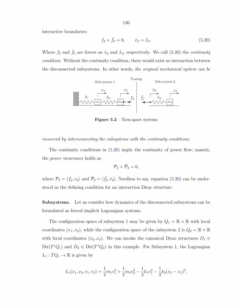
136
interactive boundaries:
f2 + f2 = 0, x2 = ˙x2. (5.20)
Where f2 and f2 are forces on x2 and ˙x2, respectively. We call (5.20) the continuity
condition. Without the continuity condition, there would exist no interaction between
the disconnected subsystems. In other words, the original mechanical system can be
TearingSub-system 1 Sub-system 2
Figure 5.2 – Torn-apart systems
recovered by interconnecting the subsystems with the continuity conditions.
The continuity conditions in (5.20) imply the continuity of power flow; namely,
the power invariance holds as
P2 + P2 = 0,
where P2 = 〈f2, v2〉 and P2 = 〈f2, v2〉. Needless to say, equation (5.20) can be under-
stood as the defining condition for an interaction Dirac structure.
Subsystems. Let us consider how dynamics of the disconnected subsystems can be
formulated as forced implicit Lagrangian systems.
The configuration space of subsystem 1 may be given by Q1 = R × R with local
coordinates (x1, x2), while the configuration space of the subsystem 2 is Q2 = R× R
with local coordinates (x2, x3). We can invoke the canonical Dirac structures D1 ∈
Dir(T ∗Q1) and D2 ∈ Dir(T ∗Q2) in this example. For Subsystem 1, the Lagrangian
L1 : TQ1 → R is given by
L1(x1, x2, v1, v2) =1
2m1v
21 +
1
2m2v
22 −
1
2k1x
21 −
1
2k2(x2 − x1)2,

137
while the Lagrangian L2 : TQ2 → R for Subsystem 2 is given by
L2(x2, x3, v2, v3) =1
2m3v
23 −
1
2k3(x3 − x2)2.
Then, we can define the generalized energy E1 on TQ1⊕T ∗Q1 byE1(x1, x2, v1, v2, p1, p2) =
p1v1+p2v2−L1(x1, x2, v1, v2), and also define the generalized energy E2 on TQ2⊕T ∗Q2
by E2(x2, x3, v2, v3, p2, p3) = p2v2 + p3v3 − L2(x2, x3, v2, v3). Although the original
system has no external force, each disconnected subsystem has an interconnection
constraint force at the interactive boundary. When viewing each system separately,
the constraint force acts as an external force on each subsystem. Again, this is be-
cause tearing always yields constraint forces at the boundaries associated with the
disconnected subsystems, as shown in Figure 5.2
Further, let X1 : TQ1⊕T ∗Q1 → TT ∗Q1 be the partial vector field, which is defined
at points (x1, x2, v1, v2, p1 = m1v1, p2 = m2v2) ∈ TQ1⊕P1 as X1(x1, x2, v1, v2, p1, p2) =
(x1, x2, p1, p2, x1, x2, p1, p2), where P1 = FL(TQ1). Similarly, let X2 : TQ2 ⊕ T ∗Q2 →
TT ∗Q2 be the partial vector field, which is defined at each point (x2, x3, v2, v3, p2 =
0, p3 = m3v3) by X2(x2, x3, v2, v3, p2, p3) = (x2, x3, p2, p3, ˙x2, x3, ˙p2, p3) ∈ TQ2 ⊕ P2,
where P2 = FL(TQ2) and we impose the consistency condition ˙p2 = 0.
Lagrange-Dirac System 1: We can formulate dynamics of System 1 in the context
of the forced implicit Lagrangian system (EL1 , D1, X1, F1) as
(X1,dEL1|TP1 − F1) ∈ D1.
The above equation may be given in coordinates by
x1 = v1, x2 = v2, p1 = −k1x1 − k2(x1 − x2), p2 = k2(x1 − x2) + f2,
and with p1 = m1v1 and p2 = m2v2.
Lagrange-Dirac System 2: Similarly, we can also formulate dynamics of System 2

138
in the context of the Lagrange-Dirac dynamical system (EL2 , D2, X2, F2) as
(X2,dE2|TP2 − F2) ∈ D2,
which may be given in coordinates by
˙x2 = v2, x3 = v3, ˙p2 = k3(x3 − x2) + f2, p3 = −k3(x3 − x2),
together with p2 = 0 and p3 = m3v3 as well as ˙p2 = 0.
In the next paragraph we will interconnect these separate systems with a Dirac
structure.
Interconnection of Distinct Dirac Structures. LetQ = Q1×Q2 = R×R×R×R
be an extended configuration space with local coordinates x = (x1, x2, x2, x3). Recall
that the direct sum of the Dirac structures is given by D1⊕D2 on T ∗Q. The constraint
distribution due to the interconnection is given by
ΣQ(x) = v ∈ TxQ | 〈ωQ(x), v〉 = 0,
where ωQ = dx2 − dx2 is a one-form on Q. On the other hand, the annihilator
ΣQ ⊂ T ∗Q is defined by
ΣQ(x) = f = (f1, f2, f2, f3) ∈ T ∗xQ | 〈f, v〉 = 0 and v ∈ ΣQ(x).
It follows from this codistribution that f2 = −f2, f1 = 0, and f3 = 0. Hence, we
obtain the conditions for the interconnection given by (5.20); namely, f2 + f2 = 0 and
v2 = v2. Let Σint = (TπQ)−1(ΣQ) ⊂ TT ∗Q and let Dint be defined as in (5.8). Finally
we derive the interconnected Dirac structure D on T ∗Q given by
D = (D1 ⊕D2) Dint.

139
Interconnection. Now, let us see how the forced implicit Lagrangian systems,
namely (EL1 , D1, X1, F1) and (EL2 , D2, X2, F2), can be interconnected through Dint
to yield a single implicit Lagrangian system. Define the Lagrangian L : TQ→ R for
the interconnected system by L = L1 +L2, and hence the generalized energy is given
by EL = EL1 + EL2 : TQ⊕ T ∗Q → R. Let ∆Q = (TQ1 × TQ2) ∩ Σint. Set a partial
vector field by X = X1 ⊕ X2 : TQ ⊕ T ∗Q → TT ∗Q, which is defined at points in
∆Q ⊕ P such that P = FL(∆Q).
Finally, the interconnected system is given by (EL, D,X), where X satisfies
(X(q, v, p),dEL(q, v, p)|TP ) ∈ D(q, p)
for each (q, p) = FL(q, v) with (q, v) ∈ ∆Q.
The Lagrange-d’Alembert-Pontryagin Principle. Additionally the intercon-
nected system is known to satisfy the Lagrange-d’Alembert-Pontryagin principle:
δ
∫ b
a
L1(x1, x2, v1, v2) + p1(x1 − v1) + p2(x2 − v2)
+ L2(x2, x3, v3) + p2( ˙x2 − v2) + p3(x3 − v3) dt = 0,
for all δx2 = δx2, for all δv and δp, and with v2 = v2.
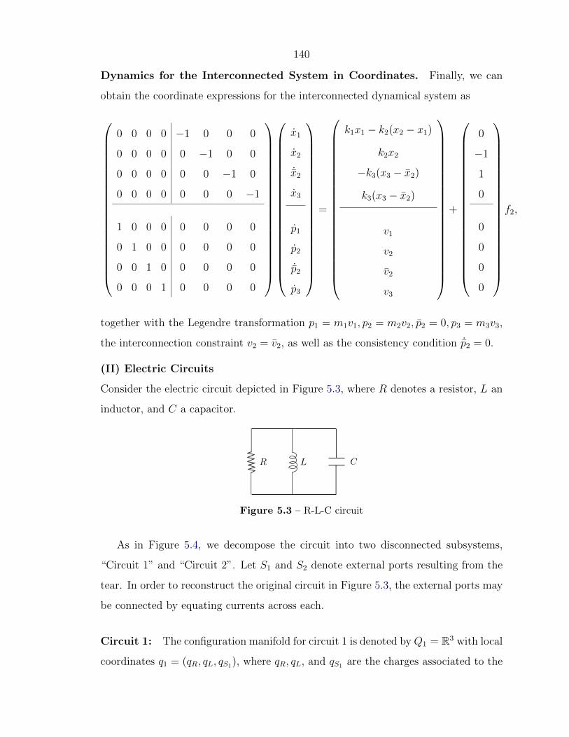
140
Dynamics for the Interconnected System in Coordinates. Finally, we can
obtain the coordinate expressions for the interconnected dynamical system as
0 0 0 0 −1 0 0 0
0 0 0 0 0 −1 0 0
0 0 0 0 0 0 −1 0
0 0 0 0 0 0 0 −1
1 0 0 0 0 0 0 0
0 1 0 0 0 0 0 0
0 0 1 0 0 0 0 0
0 0 0 1 0 0 0 0
x1
x2
˙x2
x3
p1
p2
˙p2
p3
=
k1x1 − k2(x2 − x1)
k2x2
−k3(x3 − x2)
k3(x3 − x2)
v1
v2
v2
v3
+
0
−1
1
0
0
0
0
0
f2,
together with the Legendre transformation p1 = m1v1, p2 = m2v2, p2 = 0, p3 = m3v3,
the interconnection constraint v2 = v2, as well as the consistency condition ˙p2 = 0.
(II) Electric Circuits
Consider the electric circuit depicted in Figure 5.3, where R denotes a resistor, L an
inductor, and C a capacitor.
Figure 5.3 – R-L-C circuit
As in Figure 5.4, we decompose the circuit into two disconnected subsystems,
“Circuit 1” and “Circuit 2”. Let S1 and S2 denote external ports resulting from the
tear. In order to reconstruct the original circuit in Figure 5.3, the external ports may
be connected by equating currents across each.
Circuit 1: The configuration manifold for circuit 1 is denoted by Q1 = R3 with local
coordinates q1 = (qR, qL, qS1), where qR, qL, and qS1 are the charges associated to the

141
Figure 5.4 – Disconnected circuits
resistor R, inductor L, and port S1. Kirchhoff’s circuit law is enforced by applying a
constraint distribution ∆Q1 ⊂ TQ1 known as the KCL distribution to Circuit 1. The
distribution, ∆Q, is defined for each q1 = (qR, qL, qS1) ∈ Q1 by the subspace:
∆Q1(q1) = v1 = (vR, vL, vS1) ∈ Tq1Q1 | vR − vL − vS1 = 0,
where v1 = (vR, vL, vS1) denotes the current vector at each q1, while the KVL con-
straint is given by its annihilator ∆Q1. Then, we can naturally define the induced
Dirac structure D1 on T ∗Q1 from ∆Q1 as before.
The Lagrangian for Circuit 1, namely, L1 on TQ1, is given by
L1(q1, v1) =1
2L1v
2L,
which is degenerate. Define the generalized energyEL1 on TQ1⊕T ∗Q1 byEL1(q1, v1, p1) =
〈p1, v1〉 −L1(q1, v1) on TQ1⊕ T ∗Q1. Circuit 1 also has the external force field due to
the resistor FR,1 : TQ1 ⊕ T ∗Q1 → R as
FR(q1, v1, p1) = (−RvR)dqR,
as well as a force on the variable S2 denoted by F1,port : TQ ⊕ T ∗Q → T ∗Q1. Now,
we can set up the implicit Lagrangian system (EL1 , D1, X1, FR,1 + F1,port) where X1
is a partial vector field which satisfies
(X1(q1, v1, p1), (dEL1 − F1 − F1,port)(q1, v1, p1)|TP1) ∈ D1(q1, p1),

142
where (q1, p1) = FL1(q1, v2) and (q1, v1) ∈ ∆Q(q1).
Circuit 2: The configuration manifold for Circuit 2 is Q2 = R2 with local coordi-
nates q2 = (qS2 , qC), where qS2 is the charge through the port S2 and qC is the charge
stored in the capacitor. The KCL distribution is given for each q2 by
∆2(q2) = v2 = (vS2 , vC) ∈ Tq2Q2 | vC − vS2 = 0,
and the KVL space is given by the annihilator ∆2(q2). This gives us the Dirac
structure D2 on T ∗Q2. Set the Lagrangian L2 : TQ2 → R for Circuit 2 to be
L2 =1
2Cq2C ,
and so the generalized energy EL2(q2, v2, p2) = 〈p2, v2〉 − L2(q2, v2). Circuit 2 has the
external force field due to the port F2,port. Then, we can formulate the Lagrange-
Dirac dynamical system (EL2 , D2, X2, F2,port) where X2 is a partial vector field which
satisfies
(X2(q2, v2, p2), (dEL2 − F2,port)(q2, v2, p2)|TP2) ∈ D2(q2, p2),
on point (q2, p2) = FL2(q2, v2) when (q2, v2) ∈ ∆Q2(q2).
The Interaction Dirac Structure. Set Q = Q1 ×Q2 and set
ΣQ = v = (v1, v2) ∈ TQ | vS1 = vS2.
By the tangent lift Σint = Tπ−1Q (ΣQ), we can define the interaction Dirac structure,
Dint = Σint ⊕ Σint,

143
which is denoted, in local coordinates, by
Dint = (q1, q2, p1, p2, α1, α2, w1, w2) ∈ TT ∗Q⊕ T ∗T ∗Q |
qS1 = qS2 = 0, w1 = 0, w2 = 0, (α1, α2) ∈ span(dqS1 − dqS2).
The Interconnected Circuit. Now, we can develop the interconnected Dirac
structure
D = (D1 ⊕D2) Dint,
as the Dirac structure induced from the constraint space
∆Q = (∆1 ×∆2) ∩ Σint,
which is given, in coordinates (q1, q2) = (qR, qL, qS1 , qS2 , qC), by
∆(q1, q2) = (v1, v2) = (vR, vL, vS1 , vS2 , vC) | vR − vL − vC = 0, vS1 = vS2 , vS1 = vC.
Set the Lagrangian for the interconnected system as L = L1 +L2 and the external
force field F = FR. Set also EL = EL1 + EL2 . The interconnected Lagrange-Dirac
dynamical system is given by the quadruple (EL, D,X, F ), which satisfies
(X(q, v, p), (dEL − F )(q, v, p)|TP ) ∈ D(q, p),
for each (q, p) = FL(q, v).
(III) A Ball Rolling on Rotating Tables
Consider the mechanical system depicted in Figure 5.5, where there are two rotating
tables and a ball is rolling on one of the tables without slipping. We assume the
system is conservative and the gears are linked by a no-slip constraint. Finally, we
assume the external torque is constant. Let I1 and I2 be moments of inertia for
the tables. We will now decompose the system into distinct three subsystems; (1) a
rotating (small) table, (2) a rotating (large) table, and (3) a rolling ball.

144
system 1system 2system 3
Figure 5.5 – A rolling ball on rotating tables without slipping
System 1. The configuration manifold for System 1 is the circle, Q1 = S1. The
Lagrangian is the rotational kinetic energy of the system given by
L1(s1, s1) =I1
2s2
1.
We employ the canonical Dirac structure on T ∗Q1 given by:
D1 = (s1, ps1 , αs1 , ws1) | s1 = ws1 , ps1 + αs1 = 0.
System 2. The configuration manifold for System 2 is also the circle, Q2 = S1 and
the Lagrangian is again the rotational kinetic energy
L2(s2, s2) =I2
2s2
2.
Again, we have the canonical Dirac structure
D2 = (s2, ps2 , αs2 , ws2) | s2 = ws2 , ps2 + αs2 = 0.
System 3. System 3 is a rolling sphere of uniform density and radius 1. The
sphere moves in space by changing its position and orientation relative to a reference
configuration. The configuration manifold is given by the special Euclidean group
Q3 = SE(3), which we parameterize as (R, u) where R ∈ SO(3), u ∈ R3. Following
[MR99], let β be the set of points of the sphere in the reference configuration. For
configuration (R, u) ∈ Q3, a point x ∈ β is transformed into R3 by the action (R, u) ·

145
x = (R · x) + u. The Lagrangian is given by the kinetic energy as
L3(R, u, R, u) =
∫β
ρ
2‖Rx+ u‖2dx,
where ‖Rx+ u‖2 = xT RT Rx+ 2xT RT u+ u2. We use body coordinates such that the
center of the sphere in the reference configuration is at the origin so that∫βxdx = 0.
Substituting these relations, the above Lagrangian is
L3 =
∫β
ρ
2
(xT RT Rx+ u2
)dx.
Setting m3 =∫βρdx = 4
3πρ and noting that
∫βxixjdx = 0 when i 6= j, one finally
obtains
L3 =m3
2
(tr(RT R) + u2
).
Since the motion along the z-direction is constrained so that the ball does not leave
the plane of table 2, we have the (holonomic) constraint
∆Q3 = (R, u) | u3 = 0.
This yields the induced Dirac structure
D3 = (δR, δu, δpR, δpu, αR, αu, wR, wu) ∈ TT ∗Q3 ⊕ T ∗T ∗Q3 |
δu3 = 0, δu = wu, δR = wR, δpR + αR = 0, δpu + αu = λdz for some λ ∈ R.
Interaction Dirac Structure. Let Q = Q1×Q2×Q3. In order to interconnect the
three subsystems, we need to impose the constraints due to the no-slip conditions.
By left trivialization we interpret TS1 as S1 × R. The interconnection constraint
between System 1 and System 2 is given by
ΣQ,1 = (s1, s2, R, u) ∈ TQ | s1 + s2 = 0

146
and with its annihilator
ΣQ,1 = span(ω1)
where ω1 = ds1−ds2. This constraint ensures that the gears rotate (without slipping)
at the same speed in opposite directions.
Next, we consider the interconnection constraint between Systems 2 and 3. Note
that the velocity of a point located at the bottom of the sphere is given byv1
v2
v3
= RRT ·
0
0
−1
+ u.
Note also that a point rotating on the gear of System 2 with the axle taken to be the
origin has velocity v′1
v′2
=
0 −s2
s2 0
· x
y
.
So the no-slip condition between System 2 and 3 is given by
ΣQ,2 = (s1, s2, R, u) ∈ TQ | i · (−RRT · k + u) = −s2 · u2, j · (−RRT · k + w) = s2 · u1,
where i, j,k are the basis on R3. Set the interconnection constraint distribution
ΣQ = ΣQ,1 ∩ ΣQ,2,
together with its annihilator ΣQ = ΣQ,1 + ΣQ,2. Then, one can define Σint =
(TπQ)−1(ΣQ) and with its annihilator Σint. The interaction Dirac structure is given
by
Dint = Σint ⊕ Σint.

147
The Interconnected Lagrange-Dirac System. The Dirac structure for the in-
terconnected system is given by
D = (D1 ⊕D2 ⊕D3) Dint.
Note that D is defined by the canonical two-form on T ∗Q and the distribution
∆Q = (TQ1 ⊕ TQ2 ⊕∆3) ∩ Σint,
and also that the annihilator is given by
∆Q = ∆Q3+ Σint.
Letting L = L1 +L2 +L3, the dynamics of the interconnected Lagrange-Dirac system
is given by (EL, D,X), which satisfies
(X(q, v, p), dEL(q, v, p)|TP ) ∈ D(q, p),
where X : TT ∗Q ⊕ T ∗T ∗Q → TT ∗Q is a partial vector field, defined at points
(q, v, p) ∈ TQ ⊕ T ∗Q such that (q, p) = FL(q, v) with (q, v) ∈ ∆Q, and EL : TQ ⊕
T ∗Q→ R is the generalized energy of L.
5.6 Conclusions and Future Work
We hope to have shown how interaction Dirac structures can be used in a variety of
systems. Specifically, we used the tensor product of Dirac structures, , to define
the notion of interconnection of Dirac structures and derive interconnected implicit
Lagrangian systems. This process can be repeated n-fold due to the associativity
of . This enables us to understand large heterogenous systems by decomposing
them and keeping track of the relevant interaction Dirac structures. We also clarified
how the LAP principle of an interconnected system can be decomposed into varia-
148
tional equations on separate subsystems. Lastly, we demonstrated our theory with
some examples. The result is a geometrically intrinsic framework for analyzing large
heterogenous systems through tearing and interconnection.
We hope that the framework provided here can be explored further and we are
specifically interested in the following areas for future work:
• The use of more general interaction Dirac structures such as those associated
with gyrators, motors, magnetic couplings, and so on (in this paper, we mostly
studied interaction Dirac structures of the form Σint ⊕ Σint). For examples of
these more general interconnections, see, for instance, [WC77, Yos95].
• Reduction and symmetry for interconnected Lagrange-Dirac systems ([YM07b],
[YM09]). In particular, the use of the curvature tensor of a principal connec-
tion in reduction theory is related to the interaction Dirac structures mentioned
in the last bullet [CMR01]. We conjecture that such interaction Dirac struc-
tures can be derived from reducing a Lagrangian we would call the interaction
Lagrangian.
• Applications to complicated systems such as guiding central motion problems,
multibody systems, fluid-structure interactions, passivity controlled intercon-
nected systems, etc. (See, for example, [Lit83, Fea87, Yos95, VdS96] and
[OvdSME02].)
• The integrability condition for the Dirac tensor product. As to the integra-
bility condition for Dirac structures, see [Dor93] and [DVDS98]. For the link
with composition of Dirac structures as well as with symplectic categories, see
[Wei09].
• Discrete-time versions of interconnection and . By discretizing the Hamilton-
Pontryagin principle one arrives at a discrete mechanical version of Dirac struc-
tures (see [BRM09] and [LO11]). A discrete-time version of could allow for
notions of interconnection of variational integrators.
149
• Finally, introducing noise and stochasticity into mechanical systems is at the
forefront of research in geometric mechanics. There are two major camps on
this issue. That of [CJL08] allows noise to enter the system by making the
the Hamiltonian or Lagrangian a random variable. The other camp allows
stochasticity to enter by generalizing ideas from quantization of Feynman’s path
integral, and extremizing the expected value of a “random path”. This was
successfully carried out in the case of Navier-Stokes fluids in [NYZ81]. In any
case, the symplectic structures involved in these formulations could be replaced
with Dirac structures, thus providing an understanding of how to add noise to
interconnected systems.
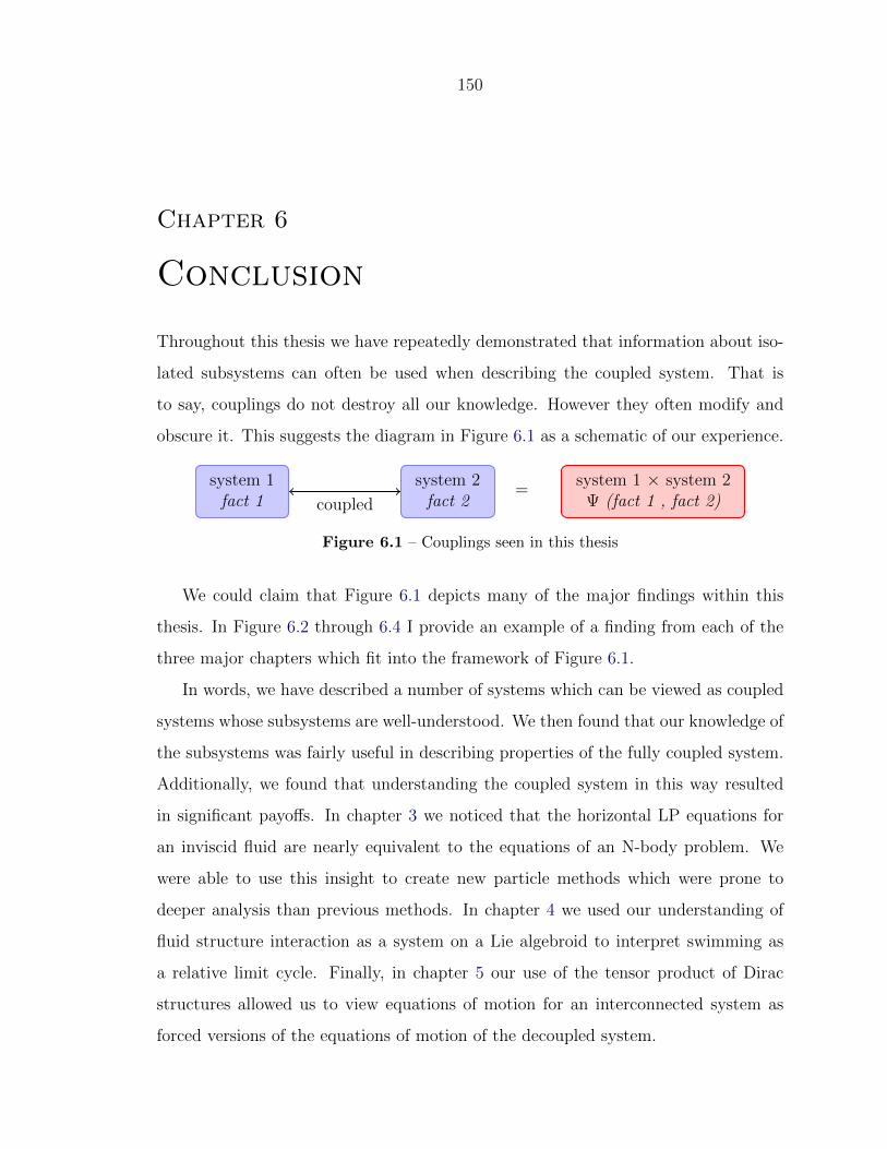
150
Chapter 6
Conclusion
Throughout this thesis we have repeatedly demonstrated that information about iso-
lated subsystems can often be used when describing the coupled system. That is
to say, couplings do not destroy all our knowledge. However they often modify and
obscure it. This suggests the diagram in Figure 6.1 as a schematic of our experience.
system 1fact 1
system 2fact 2coupled
=system 1 × system 2
Ψ (fact 1 , fact 2)
Figure 6.1 – Couplings seen in this thesis
We could claim that Figure 6.1 depicts many of the major findings within this
thesis. In Figure 6.2 through 6.4 I provide an example of a finding from each of the
three major chapters which fit into the framework of Figure 6.1.
In words, we have described a number of systems which can be viewed as coupled
systems whose subsystems are well-understood. We then found that our knowledge of
the subsystems was fairly useful in describing properties of the fully coupled system.
Additionally, we found that understanding the coupled system in this way resulted
in significant payoffs. In chapter 3 we noticed that the horizontal LP equations for
an inviscid fluid are nearly equivalent to the equations of an N-body problem. We
were able to use this insight to create new particle methods which were prone to
deeper analysis than previous methods. In chapter 4 we used our understanding of
fluid structure interaction as a system on a Lie algebroid to interpret swimming as
a relative limit cycle. Finally, in chapter 5 our use of the tensor product of Dirac
structures allowed us to view equations of motion for an interconnected system as
forced versions of the equations of motion of the decoupled system.

151
EL equations on Qpart
Hamilton’s Principle
Inviscid fluid equations on Ereduced variational principle
coupling via the Lagrangian =LP equations on TQpart ⊕ E
LP-variational principle
Figure 6.2 – A coupling described in chapter 3
Ideal Fluidequivalent to geodesicsequations on Dµ(M)
Rigid Bodyequivalent to geodesicequations on SE(3)
coupling via boundary condition =
Rigid body immersedin an ideal fluid
equivalent to geodesicequations on a Lie Groupoid
Figure 6.3 – A coupling described in chapter 4
Dirac systemwith structure D1
another Dirac systemwith structure D2
coupling via Dint =Dirac system
with structure (D1 ⊕D2) Dint
Figure 6.4 – A coupling described in chapter 5

152
At this point we hope the last paragraph of the introduction to this thesis appears
to make a sensible claim. For the convenience of the reader we will repeat some of it
here. Couplings may destroy desirable properties of subsystems, but one should never
lose hope. It is not uncommon for the beautiful aspects of the subsystems to be rein-
carnated as new creatures in the coupled system. Working to find these reincarnations
can have significant benefits.

153
Index
adjoint bundle, 17
Adjoint Maps (AD , Ad, and ad), 14
boundary conditions
for particle methods, 59
bowtie product, 122
connection
covariant derivative, 11
consistency, 59
covariant derivative, 11
curvature tensor
for subgroups, 31
general, 19
Diakoptics, 102
Dirac structure
composition of, 126
interconnection of, 125
linear, 105
manifold, 105
morphism, 106
Dirac structures
direct sum, 119
tensor product, 121
dual algebroid, 88
Euler-Lagrange equations, 10
forced, 89
Euler-Poincare equation, 16
Eulerian description of fluids, 22
force
for a Lagrangian system on a Lie
algebroid, 89
for Dirac systems, 113
for implicit Lagrangian systems, 113
groupoid, 84
Hamilton-Pontryagin principle, 111
harmonic oscillator, 112
with damping, 115
horizontal distribution, 30
horizontal lift, 30
general, 19
implicit Euler–Lagrange equations, 111
implicit Lagrangian system, 110
induced Dirac structure, 108
inner automorphism, 14
interaction constraint Dirac structure,
116

154
interconnection of variational principes,
133
isotropy subgroup, 32
Jacobi identity, 13
Kaluza-Klein Formalism, 20
Koszul’s formula, 12, 15
Lagrange-d’Alembert-Pontryagin prin-
ciple, 113
Lagrange-Dirac dynamical system, 110
Lagrangian
on a Lie algebroid, 88
Lagrangian description of fluids, 22
LC circuit, 140
left trivialization, 66
left trivializing diffeomorphism, 14
Lie algebra, 13
Lie algebroid, 86
morphism, 94
Lie groupoid, 84
morphism, 93
pair groupoid, 85
Lie groups, 13
as groupoids, 85
mass-spring system, 135
motion map, 99
Poisson structure
on a Lie algebroid, 88
principal bundle, 28
principal connection, 29
for subgroups, 29
general, 18
reconstruction method, 34
reduction
by SE(3), 93
by a subgroup, 28
by particle relabeling symmetry, 70
on a Lie algebroid, 90
with forces, 90
right trivialization, 66
rigid embeddings, 65
rigid-body equations
on SE(3), 68
on SO(3), 16
rolling constraint, 143
shape space, 86
vertical distribution, 30
viscous force, 80
155
Bibliography
[ABM06] E Afshari, H S Bhat, and J E Marsden. Extremely wideband signal
shaping using one- and two-dimensional nonuniform nonlinear trans-
mission lines. Journal of Applied Physics, 99:1–16, 2006.
[AK92] V I Arnold and B A Khesin. Topological Methods in Hydrodynamics,
volume 24 of Applied Mathematical Sciences. Springer Verlag, 1992.
[AM00] R Abraham and J E Marsden. Foundation of Mechanics. American
Mathematical Society, 2nd edition, 2000.
[AMR09] R Abraham, J E Marsden, and T S Ratiu. Manifolds, Tensor Analysis,
and Applications, volume 75 of Applied Mathematical Sciences. Spinger,
3rd edition, 2009.
[Arn66] V I Arnold. Sur la geometrie differentielle des groupes de lie de dimeni-
sion infinie et ses applications a l’hydrodynamique des fluides parfaits.
Annales de l’Institute Fourier, 16:316–361, 1966.
[AS02] S Atluri and S Shengping. The meshless local petrov-galerkin method:
A simple and less-costly alternative to the finite element and boundary
element methods. Computational Mechanics, 22:348–372, 2002.
[AS05] S Alben and M J Shelley. Coherent locomotion as an attracting state for
a free flapping body. Proceedings of the National Academy of Sciences
of the United States of America, 102(32):11163–11166, August 2005.
156
[BC97] A M Bloch and P E Crouch. Representations of Dirac structures on
vector spaces and nonlinear LC circuits. In Proc. Sympos. Pure Math,
volume 64, pages 103–117. American Mathematical Society, 1997.
[BK09] R. Wendt B. Khesin. The Geometry of Infinite-Dimensional Groups,
volume 51 of 3. Folge / A Series of Modern Surveys in Mathematics.
Springer Verlag, 2009.
[Bla00] G Blankenstein. Implicit Hamiltonian Systems: Symmetry and Inter-
connection. PhD thesis, University of Twente, 2000.
[Ble81] D Bleeker. Gauge Theory and Variational Principles, volume 1 of Ad-
vanced Graduate-level Text. Springer, 1981.
[Blo03] A M Bloch. Nonholonomic Mechanics and Control, volume 24 of In-
terdisciplinary Applied Mathematics. Springer Verlag, 2003.
[BR03] H Bursztyn and O Radko. Guaged equivalence of Dirac structures and
symplectic groupoids. Ann. Inst. Fourier, 53:309–337, 2003.
[Bra71] R K Brayton. Mathematical Aspects of Electrical Networks, chapter
Nonlinear Reciprical Networks, pages 1–15. American Mathematical
Society, 1971.
[BRM09] N Bou-Rabee and J E Marsden. Hamilton-pontryagin integrators on lie
groups: Introduction and structure preserving properties. Foundations
of Computational Mathematics, 9:197–219, 2009.
[CBL+02] D A Chang, A M Bloch, N Leonard, J E Marsden, and C Woolsey. The
equivalence of controlled Lagrangian and Hamiltonian systems. Control
and the Calculus of Variations, 8:393–422, 2002.
[CDK87] L O Chua, C A Desoer, and D A Kuh. Linear and Nonlinear Circuits.
McGraw-Hill, 1987.

157
[Cho73] A Chorin. A numerical study of slightly viscous flow. Journal of Fluid
Mechanics, 57:785–796, 1973.
[Cho94] A Chorin. Vorticity and turbulence, volume 103 of Applied Mathemat-
ical Sciences. Springer, 1994.
[CJL08] Ortega J P Cami J L. Stochastic Hamiltonian dynamical systems.
Reports on Mathematical Physics, 61(1):65–122, 2008.
[CMR01] H Cendra, J E Marsden, and T S Ratiu. Lagrangian Reduction by
Stages, volume 152 of Memoirs of the American Mathematical Society.
American Mathematical Society, 2001.
[CnNdCS07] J F Carinena, J M Nunes da Costa, and P Santos. Reduction of
Lagrangian mechanics on Lie algebroids. Journal of Geometry and
Physics, 57:977–990, 2007.
[Cou90] T J Courant. Dirac manifolds. Transactions of the American Mathe-
matical Society, 319:631–661, 1990.
[CvDSBn07] J Cervera, A J van Der Schaft, and A Banos. Interconnection of port-
Hamiltonian systems and composition of Dirac structures. Automatica,
43:212–225, 2007.
[CW88] T J Courant and A Weinstein. Beyond Poisson structures. In Action
Hamiltoniennes de groupes. Troiseme theorieme de Lie (Lyon 1986),
volume 27 of Travaux en Cours, pages 39–49. Hermann, 1988.
[dLMM05] M de Leon, J C Marrero, and E Martınez. Lagrangian submanifolds
and dynamics on lie algebroids. Journal of Physics A: Mathematical
and General, 38(24):R241, 2005.
[Dor93] I Dorfman. Dirac structures and integrability of nonlinear evolution
equations. (Nonlinear Science:Theory and Applications) . Wiley & Sons
Ltd., 1993.

158
[DVDS98] M Dalsmo and A J Van Der Schaft. On representations and integrabil-
ity of mathematical structures in energy-conserving physical systems.
Society for Industrial and Applied Mathematics Journal on Control and
Optimization, 37(1):54–91, 1998.
[DW04] J P Dufour and A Wade. On the local structure of Dirac manifolds.
arXiv:math/0405257, 2004.
[Ebi70] D G Ebin. On the space of Riemannian metrics. Symposium on Pure
Mathematics, 15:11–40, 1970.
[EM70] D G Ebin and J E Marsden. Groups of diffeomorphisms and the motion
of an incompressible fluid. The Annals of Mathematics, 92:102–163,
1970.
[Fea87] R Featherstone. Robot Dynamics Algorithms. Kluwer Academic, 1987.
[GBR09] F Gay-Balmaz and T S Ratiu. The geometric structure of complex
fluids. Advances in Applied Mathematics, 42(2):176–275, 2009.
[GH83] J Guckenheimer and P Holmes. Nonlinear oscillations, dynamical sys-
tems, and bifurcations of vector fields. Springer, 2nd edition, 1983.
[GL98] F C Gunther and W K Liu. Implementation of boundary conditions
for meshless methods. Computational Methods in Applied Mechanics
and Engineering, 163:205–230, 1998.
[GM77] R A Gingold and J J Monaghan. Smoothed particle hydrodynamics :
Theory and application to non-spherical stars. Monthly Notices of the
Royal Astronomical Society, 181:375–389, 1977.
[GM82] R A Gingold and J J Monaghan. Kernel estimates as a basis for general
particle methods in hydrodynamics. Journal of Computational Physics,
46:429–453, 1982.

159
[GMP+11] E S Gawlik, P Mullen, D Pavlov, J E Marsden, and M Desbrun. Ge-
ometric, variational discretization of continuum theories. Physica D:
Nonlinear Phenomena, 240(21):1724–1760, 2011.
[Gua07] M Gualtieri. Generalized complex structures. (preprint)
arXiv:math/0703298v2, 2007.
[HLW02] E Hairer, C Lubich, and G Wanner. Geometric Numerical Integration,
Structure Preserving Algorithms for Ordinary Differential Equations,
volume 31 of Series in Computational Mathematics. Springer Verlag,
2002.
[Hol02] D D Holm. Euler-Poincare dynamics of perfect complex fluids, pages
113–167. Fields Institute, 2002.
[Hol11a] D D Holm. Geometric Mechanics Part I: Dynamics and Symmetry.
Imperial College Press, 2nd edition, 2011.
[Hol11b] D D Holm. Geometric Mechanics Part II: Rotating, Translating and
Rolling. Imperial College Press, 2nd edition, 2011.
[JR08] M Jotz and T S Ratiu. Dirac and nonholonomic reduction. (preprint)
arXiv:0806.1261v4 [math.DG], 2008.
[JY11] H O Jacobs and H Yoshimura. Interconnection and composition of
Dirac structures. In Proceedings of the 50th IEEE Conference on De-
cisions and Control, pages 928–933. IEEE, 2011.
[JYM10] H O Jacobs, H Yoshimura, and J E Marsden. Interconnection of
Lagrange-Dirac dynamical systems for electric circuits. AIP Confer-
ence Proceedings, 1281(1):566–569, 2010.
[KCDC11] K Katija, S P Colin, J O Dabiri, and J H Costello. Comparison of flows
generated by aequorea victoria: A coherent structure analysis. Marine
Ecological Progress Series, 435:111–123, 2011.

160
[Kel98] S D Kelly. The mechanics and control of robotic locomotion with ap-
plications to aquatic vehicles. PhD thesis, California Institute of Tech-
nology, 1998.
[KM00] S D Kelly and R M Murray. Modelling efficient pisciform swimming
for control. International Journal of Robust and Nonlinear Control,
10(4):217–241, 2000.
[KMRMH05] E Kanso, J E Marsden, C W Rowley, and J B Melli-Huber. Locomotion
of articulated bodies in a perfect fluid. Journal of Nonlinear Science,
15(4):255–289, 2005.
[Kro63] G Kron. Diakoptics: The Piecewise Solution of Large-Scale Systems.
McDonald, London, 1963.
[LBLT03a] J C Liao, D N Beal, G V Lauder, and M S Triantafyllou. Fish exploiting
vorticies decrease muscle activity. Science, 302:1566–1569, 2003.
[LBLT03b] J C Liao, D N Beal, G V Lauder, and M S Triantafyllou. The Karman
gait: novel body kinematics of rainbow trout swimming in a vortex
street. Journal of Experimental Biology, 206(6):1059–1073, 2003.
[Les67] J.A. Leslie. On a differential structure for the group of diffeomorphisms.
Topology, 6(2):263 – 271, 1967.
[Lit83] R G Littlejohn. Variational principles of guiding centre motion. Journal
of Plasma Physics, 29:111–125, 1983.
[Liu03] G R Liu. Mesh Free Methods: Moving Beyond the Finite Element
Method. Chemical Rubber Company Press, 2003.
[LJZ95] W K Liu, S Jun, and Y F Zhang. Reproducing kernel particle methods.
International Journal for Numerical Methods in Fluids, 20:1081–1106,
1995.

161
[LO11] M Leok and T Ohsawa. Variational and geometric structures of discrete
Dirac mechanics. Foundations of Computational Mathematics, 11:529–
562, 2011. 10.1007/s10208-011-9096-2.
[LRW+12] B Liu, L Ristroph, A Weathers, S Childress, and J Zhang. Intrinsic
stability of a body hovering in an oscillating airflow. Physical Review
Letters, 108:068103, 2012.
[LS09] F W Lawvere and S H Schanuel. Conceptual Mathematics. Cambirdge
Press, 2009.
[Luc77] B L Lucy. A numerical approach to testing the fission hypothesis.
Astronomical Journal, 82:1013–1924, 1977.
[Mac00] S MacLane. Categories for the Working Mathematician, volume 5 of
Graduate Tests in Mathematics. Springer, 2nd edition, 2000.
[Mar67] J E Marsden. A correspondence principle for momentum operators.
Canadian Mathematics Bulletin, 10:247–250, 1967.
[Mar01] E Martınez. Lagrangian mechanics on lie algebroids. Acta Applicandae
Mathematicae, 67(3):295–320, 2001.
[MMO+07] J E Marsden, G Misiolek, J P Ortega, M Perlmutter, and T S Ratiu.
Hamiltonian Reduction by Stages, volume 1913 of Lecture Notes in
Mathematics. Springer, 2007.
[MR99] J E Marsden and T S Ratiu. Introduction to Mechanics and Symme-
try, volume 17 of Texts in Applied Mathematics. Springer Verlag, 2nd
edition, 1999.
[MRR06] J B Melli, C W Rowley, and D S Rufat. Motion planning for an ar-
ticulated body in a perfect planar fluid. Society for Industrial and
Applied Mathematics Journal on Applied Dynamical Systems, 5(4):650–
669, 2006.

162
[MV91] J Moser and A P Veselov. Discrete version of some classical integrable
systems and factorization of matrix polynomials. Communications in
Mathematical Physics, 139:217–243, 1991.
[MW74] J E Marsden and A Weinstein. Reduction of symplectic manifolds with
symmetry. Reports on Mathematical Physics, 5:121–130, 1974.
[MW01] J E Marsden and M West. Discrete mechanics and variational integra-
tors. Acta Numerica, pages 357–514, 2001.
[NYZ81] T Nakagomi, K Yasue, and J Zambrini. Stochastic variational deriva-
tions of the Navier-Stokes equation. Letters in Mathematical Physics,
5(6):545–552, November 1981.
[OIT96] E Onate, S Idelsohn, and R L Taylor. A finite point method in compu-
tational mechanics: Application to convective transport and fluid flow.
International Journal of Numerical Methods in Engineering, 39:3839–
3866, 1996.
[OIZ+96] E Onate, S Idelsohn, O C Zienkiewicz, R L Taylor, and C Sacco. A
stabilized finite point method for analysis of fluid mechanics problems.
Computer Methods in Applied Mechanics and Engineering, 139:315–
346, 1996.
[OPNSR98] R Ortega, J A L Perez, P J Nicklasson, and H J Sira-Ramirez. Passivity-
based control of Euler-Lagrange systems: Mechanical, electrical, and
electromechanical applications. Communications and Control Engineer-
ing. Springer Verlag, 1st edition, 1998.
[OvdSME02] R Ortega, A J van der Schaft, B M Maschke, and G Escobar. Inter-
connection and damping assignment passivity-based control of port-
controlled Hamiltonian systems. Automatica, 38(4):585–596, 2002.
[Pay61] H M Paynter. Analysis and Design of Engineering Systems. MIT Press,
1961.

163
[Rad03] J E Radford. Symmetry, reduction and swimming in a perfect fluid.
PhD thesis, California Institute of Technology, 2003.
[SW89] A Shapere and F Wilczek. Geometry of self-propulsion at low Reynolds
number. Journal of Fluid Mechanics, 198:557–585, 1989.
[Tru91] C Truesdell. A First Course in Rational Continuum Mechanics: Gen-
eral Concepts. Academic Press, 1991.
[VdS96] A J Van der Schaft. Port-Hamiltonian systems: An introductory sur-
vey. In Proceedings of the International Conference of Mathematics,
volume 3, pages 1–27. European Mathematical Society, 1996.
[vdSM95] A J van der Schaft and B M Maschke. The hamiltonian formulation
of energy conserving physical systems with external ports. Archi fur
Elektronik und Ubertragungstechnik, 49:362–371, 1995.
[Ves88] A P Veselov. Integrable discrete-time systems and difference operators.
Functional Analysis and Applications, 22:83–94, 1988.
[VKM09] J Vankerschaver, E Kanso, and J E Marsden. The geometry and dynam-
ics of interacting rigid bodies and point vortices. Journal of Geometric
Mechanics, 1(2):223–266, 2009.
[WC77] J L Wyatt and L O Chua. A theory of nonenergic n-ports. Circuit
Theory and Applications, 5:181–208, 1977.
[Wei78] A Weinstein. A universal phase space for particles in yang-mills fields.
Letters in Mathematical Physics, 2:417–420, 1978.
[Wei95] A Weinstein. Lagrangian mechanics and groupoids. In Mechanics Day,
volume 7 of Fields Institute Proceedings, chapter 10. American Mathe-
matical Society, 1995.
[Wei09] A Weinstein. Symplectic categories. (preprint) arXiv:0911.4133v1,
2009.

164
[YJM10] H Yoshimura, H O Jacobs, and J E Marsden. Interconnection of Dirac
structures in Lagrange-Dirac dynamical systems. In Proceedings of the
20th International Symposium on the Mathematical Theory of Networks
and Systems, 2010.
[YM06a] H Yoshimura and J E Marsden. Dirac structures and implicit La-
grangian systems in electric networks. In Proceedings of the 17th In-
ternational Symposium on the Mathematical Theory of Networks and
Systems, pages 1–6, 2006.
[YM06b] H Yoshimura and J E Marsden. Dirac structures in Lagrangian me-
chanics part I: Implicit Lagrangian systems. Journal of Geometry and
Physics, 57(1):133 – 156, 2006.
[YM06c] H Yoshimura and J E Marsden. Dirac structures in Lagrangian mechan-
ics part II: Variational structures. Journal of Geometry and Physics,
57(1):209 – 250, 2006.
[YM07a] H Yoshimura and J E Marsden. Dirac Structures and the Legendre
transformation for implicit Lagrangian and Hamiltonian systems. In
Lagrangian and Hamiltonian Methods for Nonlinear Control 2006, vol-
ume 366 of Lecture Notes in Control and Information Sciences, pages
233–247. Springer Berlin/Heidelberg, 2007.
[YM07b] H Yoshimura and J E Marsden. Reduction of Dirac structures and
the Hamilton-Pontryagin principle. Reports on Mathematical Physics,
60(3):381 – 426, 2007.
[YM09] H Yoshimura and J E Marsden. Dirac cotangeant bundle reduction.
Journal of Geometric Mechanics, 1:87–158, 2009.
[Yos95] H Yoshimura. Dynamics of Flexible Multibody Systems. PhD thesis,
Waseda University, 1995.

165
[Zei91] V Zeitlin. Finite-mode analogs of 2-D ideal hydrodynamics: Co-adjoint
orbits and local canonical structure. Physica D, 49:353–362, 1991.