Geometrical aspects of local gauge symmetry

Alexandre GuayUniversity of Pittsburgh

alg39@pitt.edu

July 13, 2004

Abstract

This paper is an analysis of the geometrical interpretation of localgauge symmetry for theories of the Yang-Mills type. It concludes,at least in the case of nonrelativistic quantum mechanics, that gaugesymmetry denotes a flexibility in the local representation of nonlocalaspects of the theory.

Contents

1 Introduction 21.1 What is local gauge symmetry . . . . . . . . . . . . . . . . . . 3

2 Geometrical formulation of gauge theory 52.1 Why the principal fibre bundle formalism? . . . . . . . . . . . 5

2.1.1 Geometrical formulation of gauge potential . . . . . . . 52.1.2 On the importance of being global . . . . . . . . . . . 82.1.3 The formalism was already there . . . . . . . . . . . . 10

2.2 Presentation of the principal fibre bundle formalism . . . . . . 112.3 The gauge potential as a connection . . . . . . . . . . . . . . . 14

3 The gauge symmetry 163.1 Gauge transformations . . . . . . . . . . . . . . . . . . . . . . 163.2 Interpretation: classical physics . . . . . . . . . . . . . . . . . 173.3 Interpretation: nonrelativistic quantum mechanics . . . . . . . 18

1

3.3.1 The gauge groupoid . . . . . . . . . . . . . . . . . . . . 193.3.2 The gauge symmetry in nonrelativistic quantum me-

chanics . . . . . . . . . . . . . . . . . . . . . . . . . . . 233.4 Interpretation: relativistic quantum mechanics . . . . . . . . . 27

4 Conclusion 29

1 Introduction

In the context of physics symmetry is defined as an immunity to possiblechange.1 In other words, it is the possibility of making a change that leavessome aspect of the situation unchanged. Thus a symmetry is always rela-tive to a class of changes and what is invariable under this class must bespecified. In most contexts the application of this concept is not philosoph-ically puzzling, but in a few philosophers and physicists meet difficulties ofinterpretation. For example in quantum mechanics, if a symmetry associatestwo apparently distinct states of a system, in what cases should we identifythese two states? Obviously the answer to this question is of great impor-tance when we try to identify the ontology of physical theory. Local gaugesymmetry is one of these problematic cases. A gauge symmetry is defined asa certain class of changes that does not affect in a physically significant waythe Lagrangian. If we want to go beyond this fact and precise exactly whatdoes not change in the theory in order to conserve the empirical content ofa physical situation, we encounter conceptual problems. Is gauge symmetrythe result of a surplus of structure like it is commonly thought? If it is theresult of a surplus of structure, why is this symmetry present in all of ourbest theories modeling fundamental interaction? This last question expressmaybe the more puzzling aspect about gauge symmetry. How a surplus ofstructure could be nonarbitrary?

We believe these questions could be clarify if we develop a sufficiently richrepresentation framework of gauge theories. In such framework we can hopeto clearly distinguish between what depends from the representation andwhat depends from the the physical model, in other words we hope to identifythe pertinent ontological features associated to gauge symmetry. In thispaper, we will argue like most physicists2 that a geometrical representation

1I borrow this elegant definition to Joe Rosen [22].2For an example of the physicist point of view, see the classical paper of Daniel and

2

of gauge theories is an interesting framework for the philosophical analysis.As we will see this interpretation provide clues that in for the quantized Yang-Mills theories3 the gauge symmetry is the result of a surplus of structure; asurplus that is produced by representing locally non local features of gaugetheories. Of course I used the word “clues” and not “proof” because thegeometrical interpretation has limits that we will expose. The geometrizationprogram of physics is not advanced enough to assert firmly an interpretationof gauge symmetry.

1.1 What is local gauge symmetry

In many analysis of gauge theory philosophers limit themselves to the sim-plest case: electrodynamics. General conclusions induced from this theorycould be misleading. For example in electrodynamics the gauge field Fµν isgauge invariant. This is not generally the case. Subsequently the belief thatFµν represents the “real field” because it is a covariant field that is gaugeinvariant cannot be generally defended. Since I believe that gauge theoriesform a “natural class”, it seems clear to me that an analysis of a special casewill not do. Theories that we call gauge theories are not put in the samecategory for arbitrary reasons. They share a basic structure that incline meto believe that a good philosophical analysis should apply to all of them.4

Therefore I will focus my analysis on a wide class of gauge theories, oftencalled Yang-Mills theories. This class includes among others electrodynamicsand quantum chromodynamics.

Let us assume that we have a field theory where a matter field, repre-sented by ψ(x), is coupled to a gauge potential Aµ = Aa

µta, where ta are

generators of the gauge group forming the algebra [ta, tb] = ifabctc, wherefabc are structures constants. The local gauge symmetry implies that thistheory is unchanged, that the Lagrangian is invariant, under the following

Viallet [6].3In this paper we will put aside general relativity which is also a gauge theory. This

we will do for two reasons: 1) the ontological implication of gauge symmetry is differentthan in other theories because it affects directly space-time; 2) the quantization of generalrelativity is not enough developed for discussing the case properly.

4Like I said general relativity could be an exception.

3

transformations:

ψ(x) → V (x)ψ(x) (1)

Aaµt

a → V (x)

(Aa

µta +

i

g∂µ

)V †(x) (2)

where matrices V (x) = exp (iαa(x)ta) form a group G, where αa(x) aresmooth functions of space-time, g is the charge associated to the gauge in-teraction. Note that it is because αa(x) are explicitly function of space-timethat we call these transformations local. In this theory the field-tensor is

F aµν = ∂µA

aν − ∂νA

aµ + gfabcAb

µAcν (3)

and transforms under an infinitesimal gauge transformation as

F aµν → F a

µν − fabcαbF cµν (4)

As an example, let us take V (x) = exp(iα(x)). In this case5 the V (x) form agroup isomorphic to U(1). The gauge potential and the field tensor transformas

Aµ → Aµ +1

g∂µα(x) (5)

Fµν → Fµν (6)

We recognize here the case of electrodynamics. Since all known observablequantities are gauge invariant, it seems plausible that local gauge symmetriesare the result of a surplus of structure in the theory.6 Face with this surplus,two strategies possible:

1. We try to formulate gauge theories in a gauge invariant way.7

2. We identify the surplus, continue to work with it for pragmatic reasons,and stay careful about the interpretation of the theory.

The first strategy, though philosophically very interesting, creates a mystery.If we could work without gauge freedom, why have we formulate all theoriesabout fundamental interaction with such freedom? What are the pragmaticreasons that incline us to do so? We will see that a geometrical formulationof gauge theories could be appropriate to answer this question.

5Note that in the case the group generator is the unity matrix.6This position was recently discussed by Michael Redhead [21], but has been already

defended by Eugene P. Wigner in 1964 [26].7A good example of that is the constrained Hamiltonian formulation of electrodynamics.

See Gordon Belot [3].

4

2 Geometrical formulation of gauge theory

2.1 Why the principal fibre bundle formalism?

Even if we agree on the merits of a geometrical formulation of gauge theories,we are still faced to a number of choices on how to built such a representation.What lies at the center of these choices is how we will model geometricallyproperties that are associated with space-time but are not properties of space-time. In the case of classical gauge theories physicists massively believethat the principal fibre bundle formalism is the right one for the job. Inthis subsection I will expose three reasons for choosing this formalism; threereasons that are rarely explicit in the physics litterature.

1. In the principal fibre bundle formalism, the gauge potential is under-stood naturally as a connection. This is appealing because it modelsinteraction as a topological feature.

2. Gauge theories exhibit global aspects. The principal fibre bundle for-malism can represent these aspects.

3. The principal fibre bundle theory was already well developed whenphysicists needed it.

2.1.1 Geometrical formulation of gauge potential

The conception defended in this subsection has been influenced by MichaelAtiyah work [2]. The gauge principle (also called gauge argument) requiresthat the coupling between a free matter field and the free interacting fieldis made through the application of an operator on the matter field. Thisoperator is called a covariant derivative8:

Dµ = ∂µ − igAµ (7)

The commutator of this operator generates the field tensor (equation 3):

[Dµ, Dν ] = −igF aµνt

a (8)

8I am adopting here the position of Lyre on the gauge argument which interpret thisone as a constraint on how to couple two free field theories [13]. For more details on thegauge principle see Martin dissertation [16]. For a geometrical interpretation of the gaugeargument see Teller [23].

5

Under a gauge transformation (equation 2), the gauge potential transformsin an inhomogeneous way, in fact like a connection. This is not the case forthe field tensor:

F aµνt

a → V (x)F aµνt

aV †(x) (9)

which transforms like a vector (or tensor).Let us take seriously that Aµ could be some kind of connection. But a

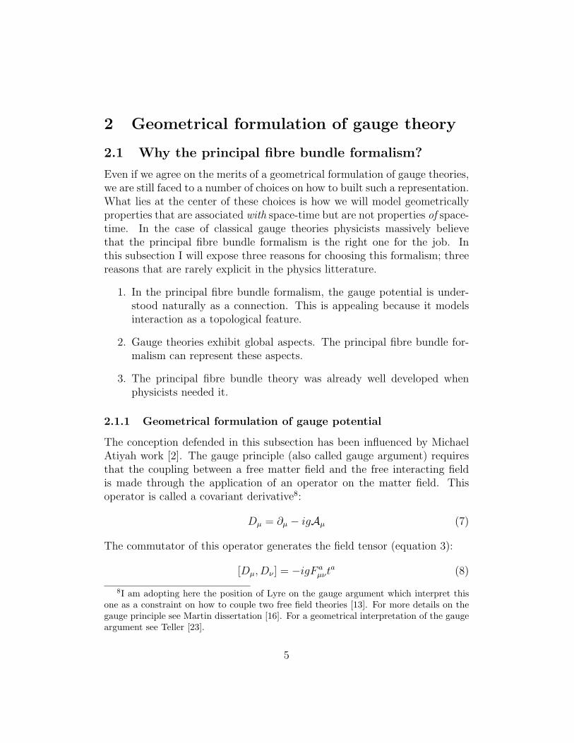
connection of what space? It is not apparently a connection of space-time. Infact, the attempt of Hermann Weyl (1918) to relates this connection to thetopology of space-time failed.9 To interpret Aµ(x) as a connection, we haveto add something to space-time (represented as a Minkowski space M4):a charge space10. Each element of this internal space will be labeled byelements g ∈ G (the gauge group). This way, gauge transformations exhaustthis internal space. See Figure 1. In general we conceive the internal space

4

Gx

x

G

M

Figure 1: Total space P .

Gx and Gy for x 6= y, x, y ∈M4 as not being indentified. In fact, we have noa priori reason to believe that property space at different point in space-timeare the same. The best we can do is to consider Gx and Gy are of the sametype since they represent properties pertinent for the same interaction. Sowe can draw the total space P as a collection of fibres.

In the absence of external field (interacting field), we consider convention-ally that all Gx can be identified to each other. I insist that this identification

9For more details see the book of Lochlainn O’Raifeartaigh [20], chapter 1.10I borrow this non standard expression to Faddeev and Slavnov, page 8 of [8].

6

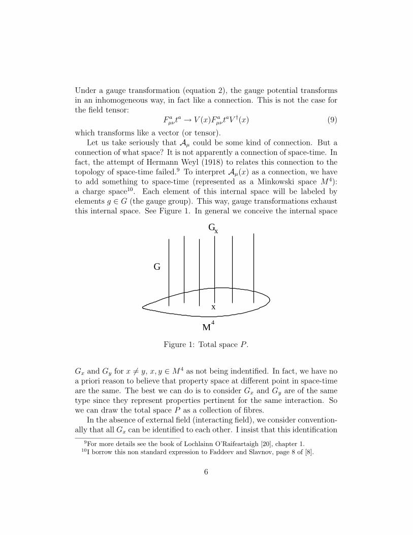
is purelly conventional. See Figure 2. In that case, we can define horizontal

G

M4

Figure 2: P without interaction.

lines (called sections) to compare points in different fibres. An interactingfield has the effect of distorting the relative alignment of fibres so no co-herent identification is possible between Gx at different point. However wewill presume that Gx and Gy can still be compared if we choose a definitepath in M4 from x to y. This identification of fibres along the path is thefamiliar notion of parallel transport. Of course we have no a priori reasonto believe that if we choose a different path from x to y, we will obtain thesame identification. This difference or “phase shift” can be viewed as thetotal curvature over the region enclosed by the two paths.

If we pass to an infinitesimal description, the field that represents theinfinitesimal shift in fibres that is produced by moving of an infinitesimalin any direction in M4 is what we call the connection. The infinitesimalcurvature depends of two directions at x and takes values in the Lie algebraof Gx. It is also an infinitesimal shift. If now we compare this situationto the case without interacting field, we note that Aµ plays the role of theconnection in the covariant derivative and Fµν the curvature. The interactingfield by mean of the field tensor modifies locally the geometry of the internalspace. This identification of fields with geometrical distortion is the heart ofEinstein’s theory of gravitation. This analogy is appealing.

In order to give a geometrical meaning to Aµ, we compared the situa-tion with an interacting field (Fµν 6= 0) to the situation in the absence ofan external field. This was not the general case. We could have chosen a

7

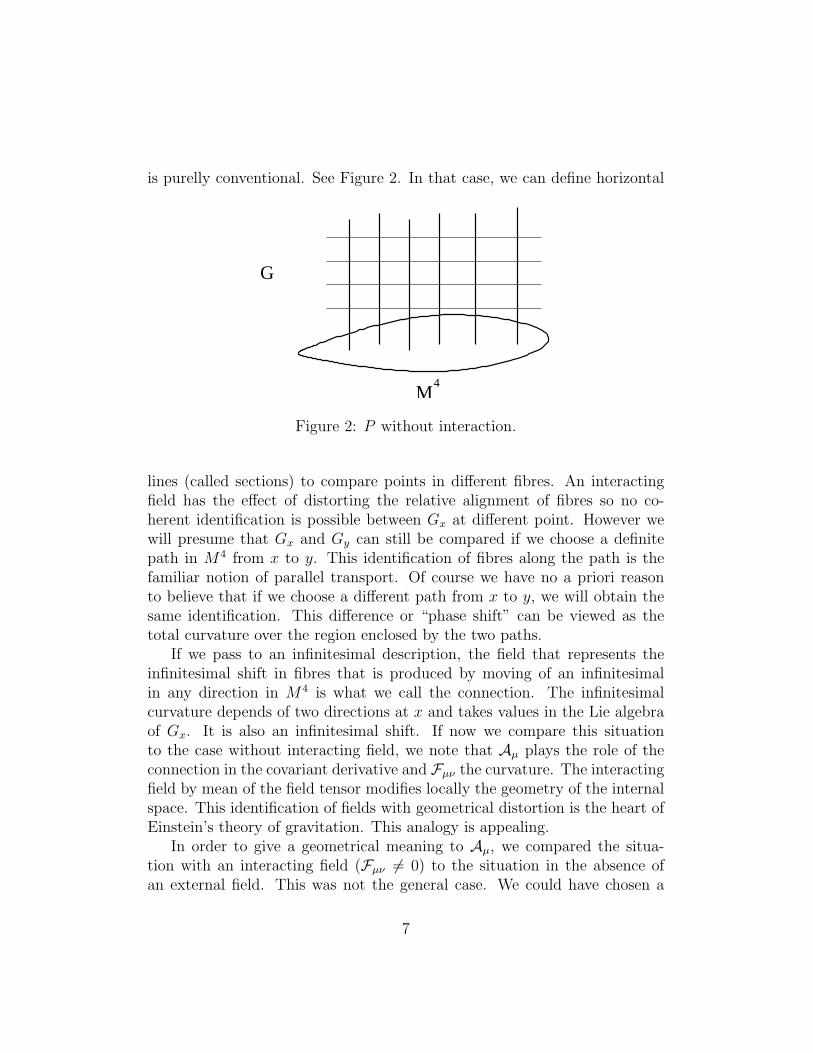
different identification of the fibres. This coherence represents the absence

Figure 3: Two identifications of the fibres (two gauges).

of field. A particular choice is called choosing a gauge and we can changefrom one choice to another by a gauge transformation. In that sens a gaugetransformation is a passive transformation and plays a role analogous to acoordinate transformations in Riemannian geometry. The construction thatwe just described is a special case of principal fibre bundle.

2.1.2 On the importance of being global

The second reason to choose principal fibre bundle formalism is that it canrepresent global topological features. In physics, field theories are believed tobe local, but this main line of thought does not exclude that global featurescould not be significative. In recent litterature two subjects implying globalproperties have been widly discussed: monopoles and instantons. In thissubsection I will discuss how that kind of examples have put constraints onpossible geometrisation of Yang-Mills theories. Constraints that are easilyrepresentable in the principal fibre bundle formalism.

I will illustrate my point by discussing of a particular example the Dirac’smonopole [7]. This case applies to electrodynamics but could be generalizedfor non-abelian gauge theories. For details see [28]. Let us imagine that wehave in a certain referential a magnetic monopole. In other words in thisreferential:

~E = 0, ~B =g

ρ2eρ for ρ 6= 0, (10)

8

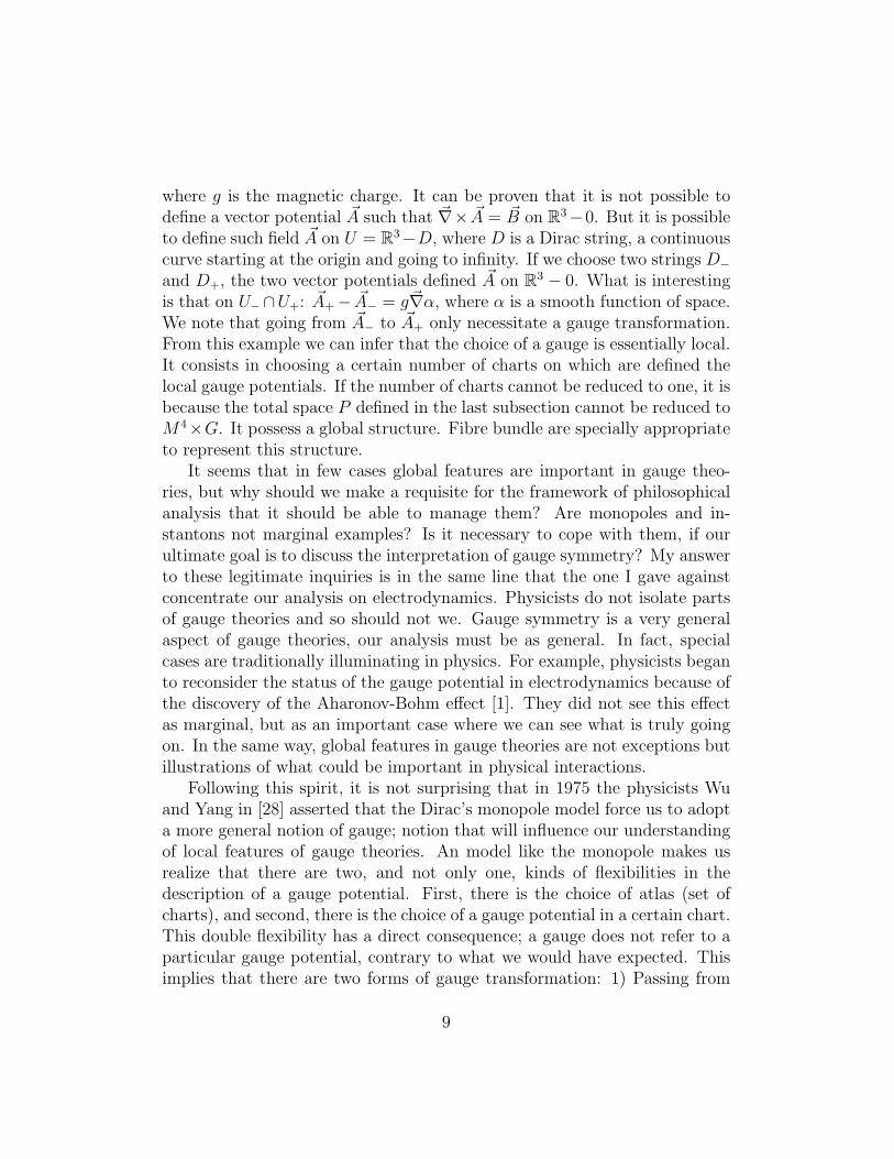
where g is the magnetic charge. It can be proven that it is not possible todefine a vector potential ~A such that ~∇× ~A = ~B on R3−0. But it is possibleto define such field ~A on U = R3−D, where D is a Dirac string, a continuouscurve starting at the origin and going to infinity. If we choose two strings D−and D+, the two vector potentials defined ~A on R3 − 0. What is interestingis that on U−∩U+: ~A+− ~A− = g~∇α, where α is a smooth function of space.We note that going from ~A− to ~A+ only necessitate a gauge transformation.From this example we can infer that the choice of a gauge is essentially local.It consists in choosing a certain number of charts on which are defined thelocal gauge potentials. If the number of charts cannot be reduced to one, it isbecause the total space P defined in the last subsection cannot be reduced toM4×G. It possess a global structure. Fibre bundle are specially appropriateto represent this structure.

It seems that in few cases global features are important in gauge theo-ries, but why should we make a requisite for the framework of philosophicalanalysis that it should be able to manage them? Are monopoles and in-stantons not marginal examples? Is it necessary to cope with them, if ourultimate goal is to discuss the interpretation of gauge symmetry? My answerto these legitimate inquiries is in the same line that the one I gave againstconcentrate our analysis on electrodynamics. Physicists do not isolate partsof gauge theories and so should not we. Gauge symmetry is a very generalaspect of gauge theories, our analysis must be as general. In fact, specialcases are traditionally illuminating in physics. For example, physicists beganto reconsider the status of the gauge potential in electrodynamics because ofthe discovery of the Aharonov-Bohm effect [1]. They did not see this effectas marginal, but as an important case where we can see what is truly goingon. In the same way, global features in gauge theories are not exceptions butillustrations of what could be important in physical interactions.

Following this spirit, it is not surprising that in 1975 the physicists Wuand Yang in [28] asserted that the Dirac’s monopole model force us to adopta more general notion of gauge; notion that will influence our understandingof local features of gauge theories. An model like the monopole makes usrealize that there are two, and not only one, kinds of flexibilities in thedescription of a gauge potential. First, there is the choice of atlas (set ofcharts), and second, there is the choice of a gauge potential in a certain chart.This double flexibility has a direct consequence; a gauge does not refer to aparticular gauge potential, contrary to what we would have expected. Thisimplies that there are two forms of gauge transformation: 1) Passing from

9

a chart to another in a overlapping region is what we call a passive gaugetransformation. 2) Passing from a gauge potential to an equivalent one inthe same chart will be an active gauge transformation. It is interesting to

B

A

B

A

Figure 4: Respectively passive and active gauge transformation between localgauge A and B.

note that in the mathematics litterature a gauge transformation always referto the active case. In the physics litterature it is the contrary. If these twokinds of transformations are clearly mathematically equivalent, they are notphilosophically the same. Usually passive transformation are considered aschanges of representation and active ones as physical changes. I will returnto this point latter in this article.

2.1.3 The formalism was already there

The two reasons I have exposed are strong motivations to choose the principalfibre bundle formalism to model classical gauge theories, but alternatives arepossible.11 The Lie groupoid is an interresting example, but it is not asdeveloped and as known as the principle fibre bundle formalism.

In 1970, the physicist A. Trautman [24] advocated for the use of fibrebundle techniques to clarify concepts often confused like relativity, symme-try, covariance, invariance and gauge or coordinate transformations. Fibrespace was already a well developed field of research in mathematics. In1930’s, H. Seifert has introduced the notion of fibre space. By 1950, thenotion of fibre space and fibre bundle had become central in the study ofalgebraic topology. The specific notion that interests us the principal fibrebundle was fully developed by the mathematician C. Ehresmann in the 50’under the influence of Cartan. It happens so often that physicists have todevelop their own mathematical tools that it must have been a relief to find

11For the historical part of this subsection, we rely on an unpublished paper by JohnMcCleary [19].

10

a mathematical theory already there when you need it. This seems to methe main reason why physicists did not produce alternative geometrical con-structions of gauge theories. The mathematics already exist and it fits theirpurposes. As a philosopher we have to be careful because it is possible thatthis formalism does not fit our purpose which is to have a clear understandingof the conceptual foundations of gauge symmetry.

2.2 Presentation of the principal fibre bundle forma-lism

In this subsection I will briefly present some essential elements of the principalfibre bundle theory applied to Yang-Mills theories. The reader is invited tonote how closely this formalism is mapping the conception I discussed in theprecedents subsections.

Definition 1 (Yang-Mills principal fibre bundle) A Yang-Mills princi-pal fibre bundle P (M4, G, π) consists of the following elements:

1. A differentiable manifold P called the total space.

2. A Minkowski manifold M4 called base space.

3. A Lie gauge group G called the fibre.12

4. A surjection π : P →M4 called projection. The inverse image π−1(x) ≡Gx

∼= G is called the fibre at x.

5. A Lie group G called the structure group, which acts on the fibre G onthe left.13

6. A set of open covering Ui of M4 with a diffeomorphism φi : Ui×G→π−1(Ui) such that πφi(x, g) = x. The map φi is called the local gaugeor local trivialization since φ−1

i maps π−1(Ui) onto the direct productUi ×G.

7. If we write φi(x, g) = φi,x(g), the map φi,x : G → Gx is a diffeomor-phism. On Ui ∩ Uj 6= ∅, we require that Sij(x) ≡ φ−1

i,xφj,x : G → G be

12In the case of Yang-Mills theories G ≡ SU(N).13What make a fibre bundle principal is that the structure group is isomorphic to the

fibre.

11

an element of the structure group G. The φi and φj are related by asmooth map Sij : Ui ∩ Uj → G such as φj(x, g) = φi(x, Sij(x)g). Sijare called transition functions or passive gauge transformations.

As you can see this definition express explicitly the notions discussed in theprecedent subsection. Note the fact that the structure group is isomorphicto the fibre will guaranty that for every passive gauge transformation therewill be an equivalent active gauge transformation. This is the geometricalimplementation of the Yang and Wu conception of a gauge.

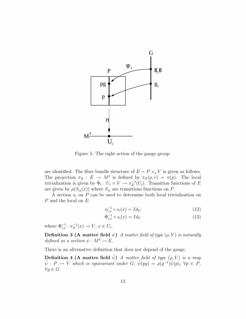
There is something that was not emphasized in the preceding discussion.Because the structure group is isomorphic to the fibre, we can define the rightaction of G on the fibre independently of local gauges. Let φi be a local gaugegiven by φ−1

i (p) = (x, gi), where p ∈ π−1(Ui) and πp = x. The right action ofG on π−1(Ui) is defined by φ−1

i (pg) = (x, gig), that is, pg = φi(x, gig) for anyg ∈ G and p = π−1(x). This definition is independent of the local gauges. Ifx ∈ Ui ∩ Uj, then

pg = φj(x, gjg) = φj(x, Sji(x)gig) = φi(x, gig) (11)

This action will be important for the groupoid description of gauge theories.In this formalism, the notion of section that we briefly used can be defined

as:

Definition 2 (A section) A section is a smooth map s : M4 → P whichsatisfies πs = idM4.

Given a section si(x) over Ui, we can define a prefered local gauge φi asfollows. For p ∈ π−1, x ∈ Ui, there is a unique element gp ∈ G such thatp = si(x)gp, then we define φi by φ−1

i (p) = (x, gp). In this local gaugethe section is expressed as si(x) = φi(x, e). This local gauge is called thecanonical local trivialization (or gauge).

We have a well defined geometrical space where the gauge potentialslive, but now we have to define the associated vector bundle appropriate forthe geometrisation of the matter field ψ(x). Given a principal fibre bundleP (M4, G, π), we may construct the associated vector bundle as follows. LetGacts on a k-dimensional vector space V on the left. Define an action of g ∈ Gon P × V by (p, v) → (pg, ρ(g)−1v), where ρ is the k-dimensional unitaryrepresentation of G. Then the associated vector bundle E(M4, G, V, P, πE)is an equivalence class P × V/G in which two points (p, v) and (pg, ρ(g)−1v)

12

i

G

π

Ui

P

p

g

i

M4

pg

φg gg g

i

Figure 5: The right action of the gauge group.

are identified. The fibre bundle structure of E = P ×ρ V is given as follows.The projection πE : E → M4 is defined by πE(p, v) = π(p). The localtrivialization is given by Φi : Ui × V → π−1

E (Ui). Transition functions of Eare given by ρ(Sij(x)) where Sij are transitions functions on P .

A section si on P can be used to determine both local trivialization onP and the local on E:

φ−1i,x si(x) = IdG (12)

Φ−1i,x si(x) = IdV (13)

where Φ−1i,x : π−1

E (x) → V , x ∈ Ui.

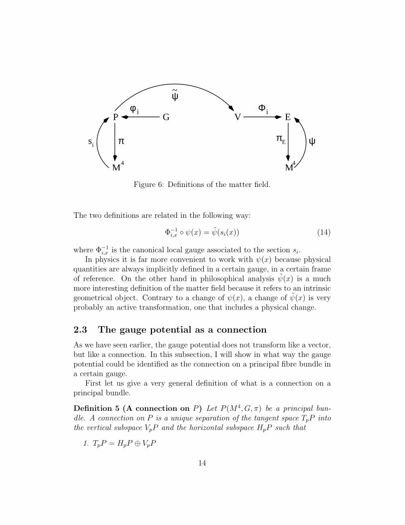
Definition 3 (A matter field ψ) A matter field of type (ρ, V ) is naturallydefined as a section ψ : M4 → E.

There is an alternative definition that does not depend of the gauge.

Definition 4 (A matter field ψ) A matter field of type (ρ, V ) is a mapψ : P → V which is equivariant under G; ψ(pg) = ρ(g−1)ψ(p), ∀p ∈ P ,∀g ∈ G.

13

~

GPi

E

πEsi ψ

Φi

π

M M4 4

Vφ

ψ

Figure 6: Definitions of the matter field.

The two definitions are related in the following way:

Φ−1i,x ψ(x) = ψ(si(x)) (14)

where Φ−1i,x is the canonical local gauge associated to the section si.

In physics it is far more convenient to work with ψ(x) because physicalquantities are always implicitly defined in a certain gauge, in a certain frameof reference. On the other hand in philosophical analysis ψ(x) is a muchmore interesting definition of the matter field because it refers to an intrinsicgeometrical object. Contrary to a change of ψ(x), a change of ψ(x) is veryprobably an active transformation, one that includes a physical change.

2.3 The gauge potential as a connection

As we have seen earlier, the gauge potential does not transform like a vector,but like a connection. In this subsection, I will show in what way the gaugepotential could be identified as the connection on a principal fibre bundle ina certain gauge.

First let us give a very general definition of what is a connection on aprincipal bundle.

Definition 5 (A connection on P ) Let P (M4, G, π) be a principal bun-dle. A connection on P is a unique separation of the tangent space TpP intothe vertical subspace VpP and the horizontal subspace HpP such that

1. TpP = HpP ⊕ VpP

14

2. A smooth vector field X on P is separated into smooth vector fieldsXH ∈ HpP and XV ∈ VpP as X = XH +XV .

3. HpgP = Rg∗HpP for arbitrary p ∈ P and g ∈ G.

The vertical subspace VpP is a subspace of TpP which is tangent to Gx at p.The third condition states that HpP and HpgP on the same fibre are relatedby a linear map Rg∗ induced by the right action of the gauge group.

With this definition of the connection, we can easily define the notionof parallel transport of a vector along a curve in M4 using the notion ofhorizontal lift.

Definition 6 (Horizontal lift) Let P (M4, G, π) be a principal bundle andlet γ : [0, 1] → M4 be a curve in M4. A curve γ : [0, 1] → P is said to be ahorizontal lift of γ if πγ = γ and if the tangent vector to γ(t) always belongsto Hγ(t)P .

These definitions imply two nice theorems that I will not prove here:

Theorem 1 Let γ : [0, 1] → M4 be a curve in M4 and let p ∈ π−1(γ(0)),then there exists a unique horizontal lift γ(t) in P such that γ(0) = p.

Corollary 1 Let γ′ be another horizontal lift of γ, such that γ′(0) = γ(0)g,then γ′(t) = γ(t)g for all t ∈ [0, 1].

We can see that this corollary implies among others things the global gaugesymmetry. A global right action does not modify the connection structureof the principal fibre bundle.

For practical reasons physicists prefer to work with an equivalent defini-tion of the connection called the Ehresmann one-form connection.

Definition 7 (A connection on P ) A connection one-form ω is a projec-tion of TpP onto the vertical component VpP ' G the Lie algebra of G. Theprojection property is summarized by the following requirements:

1. ω(v) = v, where v ∈ Vp and v ∈ G are related by the canonical isomor-phism.14

14Let v ∈ G correspond to dg(s)/ds|s=0 ∈ Te(G); the equation v(p) = d(Rgp)/ds|s=0 ∈Vp defines the canonical isomorphism between G and Vp. For more details see [4], pp359-360.

15

2. R∗gω = Adg−1ω that is for u ∈ TpP , R∗

gωpg(u) = ωpg(R∗gu) = g−1ωp(u)g.

The connection ω is independant of local gauges but Aµ are not. The relationbetween ω and Aµ is simple. For a certain Ui and a certain local gauge φi:

Ai ≡ s∗iω (15)

where s∗i is the pullback of the local section canonically related to φi. Notethat Ai is defined only on Ui. If xµ are local coordinates on Ui, then werecover the well known gauge potential

Ai ≡ (−igAaµt

adxµ)i (16)

where −i is the Lie algebra factor and g the charge associated to the interac-tion. We are now ready to attack our main question: the status of the gaugesymmetry.

3 The gauge symmetry

3.1 Gauge transformations

What is a gauge transformation in our geometrical construction? Like wesaw for the Dirac’s monopole there is not only one answer to this question.Passive and active interpretation of gauge transformations must be studied.

Let us begin with the passive viewpoint. We are looking at the same p ∈P , πp = x, but in two different local gauges (local coordinations) φi and φj.We can write that φ−1

i (p) = φ−1j (R(p)), where R is a vertical automorphism,

in other words R : π−1(x) → π−1(x), R(pg) = R(p)g, p ∈ P , g ∈ G. Thisis a consequence of the gauge independence of the right action of G. Whathappens when we pass from the gauge i to the gauge j?

the connection: ω → ω (17)

the potential: Ai = s∗iω → (R si)∗ω (18)

the matter field: ψ → ψ (19)

ψ → ρ(Sji) ψ (20)

In coordinates:

ψ(x) → V (x)ψ(x) (21)

Aaµt

a → V (x)

(Aa

µta +

i

g∂µ

)V †(x) (22)

16

This transformation is clearly a simple change of representation. To thepassive viewpoint corresponds an active one. Let us look at two pointsp,R(p) ∈ P related by the same automorphism than above. This time,we stay in the same local gauge φi. The effect of this vertical automorphismof the principqal fibre bundle is

the connection: ω → R∗ω (23)

the potential: Ai = s∗iω → s∗i (R∗ω) (24)

the matter field: ψ → R∗ψ (25)

It is now time to pass to our main objective.15

3.2 Interpretation: classical physics

In classical electrodynamics, the gauge is understood as a surplus of structure,because only Fµν is considered as a physical field (not Aµ). A necessarybut not sufficient condition to be considered a physical field is to be gaugeinvariant. We will see that this conclusion about gauge symmetry status canbe extend to all classical gauge theories.

If the meaning of gauge transformation was restricted only to the passivecase, gauge symmetry would only denote the freedom we have in choosinga representation framework (coordinations). Knowing that, we would stillhave to identify which intrinsic structures of the geometrical construction“correspond” to physical entities. If in electrodynamics the locality of inter-action and Maxwell’s equations favor that the curvature of the connection,Fµν in coordinates, is the interaction field, in non-Abelien cases things arenot that simple. In these cases Fµν is not gauge invariant. Since physicistshave a strong presumption that only gauge invariant objects can representreal entities, the active field in classical non-abelien theories could not be Fµν .On the other hand under a passive gauge transformation ω stays inchanged.

15In the conception of Yang and Wu of a gauge the difference between a global and alocal transformation is blurred. In fact, a transformation ψ → V (x)ψ for a domain ofspace-time can be interpreted as

• a local transformation measured in a gauge using the same coordination for all thedomain or

• a global transformation measured in a gauge where there is a different coordinationfor each point of the domain.

17

Apparently, the intrinsic connection could be the physical field. However,this analysis is forgetting the active partner of a gauge transformation.

If we extend the definition of gauge transformation to include active ones,the conclusion about the status of gauge symmetry does not change. Fur-thermore, since ω and ψ are not gauge invariant, we cannot defend that thetopology of the fibre bundle construction could represent a physical stateof affairs. An infinite number of connection ω represent the same physicalcontent and nothing in the fibre bundle construction helps us to choose oneof them.16

But do we have to include active transformations in the set of gauge trans-formations? I remind you that this distinction between active and passivetransformations comes directly from the analysis of models, like monopoles,with global geometrical properties. Put aside active transformations wouldunable us to understand the gauge structure of these examples. In fact,only active interpretation of gauge transformations allows gauge symmetryto have a possible physical meaning. Therefore, we should not exclude activegauge transformations without imperative reasons.

At this point our geometrical construction has permitted us to extendthe well known interpretation of gauge symmetry in electrodynamics to non-abelien classical gauge theories. Nevertheless, we are no more advanced inour understanding of the origin of this symmetry. To go beyond we willhave to examine the application of fibre bundle formalism in non-classicaldomains.

3.3 Interpretation: nonrelativistic quantum mechanics

We will examine in this subsection the semi-classical case, namely whenquantized charges particles interact with a classical external gauge field. Thiscategory is far to be exotic. Most of problems solved in non-relativisticquantum mechanics are in this class. The very well known Aharonov-Bohmeffect, much discussed in philosophy recently, falls also in this category. Thusfor the rest of this subsection, we will consider that ψ(x) is a wave function17

representing appropriately charged particles which interact with a classicalgauge field.

16Richard Healey made a similar analysis for electrodymamics in semi-classical contexts[11].

17This analysis is applicable to the case when ψ is a wave function because in thissituation the Schrodinger equation is locally gauge invariant.

18

3.3.1 The gauge groupoid

Let us return to the fibre bundle construction. If ψ(x) is representing awave function then its absolute phase is not significant. This has a directgeometrical consequence. The elements p ∈ Gx have no physical meaning,only variation between elements in different fibres have one. By defining foreach x ∈ M4 an internal space isomorphic to G, we built to much structurein the geometrical construction. Does it mean that fibre bundle formalismis useless in quantum physics? Of course not, but we have to reexamine theformalism and extract the phase invariant structure. This work has alreadybeen done by mathematicians like Ehresmann in the 1950’s, following hiswork on the concept of principal bundle. To do so, he used the groupoidtheory.18 A groupoid is a generalization of a group that is particularly handyto express local symmetries of geometrical structure. See [25] for more details.

The particular groupoid that we need is called the Ehresmann or gaugegroupoid. As we will see in this formalism above the base space we do notfind internal spaces but arrows that denote difference of internal propertiesbetween points of space-time.

Definition 8 (The gauge groupoid) Let P (M4, G, π) be a principal bun-dle. Let G act on P×P to the right by (p2, p1)g = (p2g, p1g); denote the orbitof (p2, p1) by 〈p2, p1〉 and the set of orbits by P×P

G, then the gauge groupoid

consists of two set Ω = P×PG

and M4, called respectively the groupoid and thebase, together with two maps α : 〈p2, p1〉 7→ π(p1) and β : 〈p2, p1〉 7→ π(p2),called respectively the source and the target, a map ε : M4 → Ω;x 7→ x =〈p, p〉, called the object inclusion map, and of a partial multiplication in Ω de-fined on the set Ω×Ω = (〈p3, p

′2〉, 〈p2, p1〉) ∈ Ω×Ω |α(〈p3, p

′2〉) = β(〈p2, p1〉)

〈p3, p′2〉〈p2, p1〉 = 〈p3, p1δ(p

′2, p2)〉 (26)

where δ : P × P → G is the map (pg, p) 7→ g.

The gauge groupoid is a geometrical construction very close to the prin-cipal fibre bundle. The main difference is that information about particularpoints in fibres is lost in the groupoid, only relative relations between fibresis kept. Thus the gauge groupoid seems more in accordance with quantumtheory.

18To my knowledge the first that proposed using groupoid in a physical context wasMeinhard Mayer in 1988 [17].

19

1

GG

G

M4

p

pp

2

p’2

3

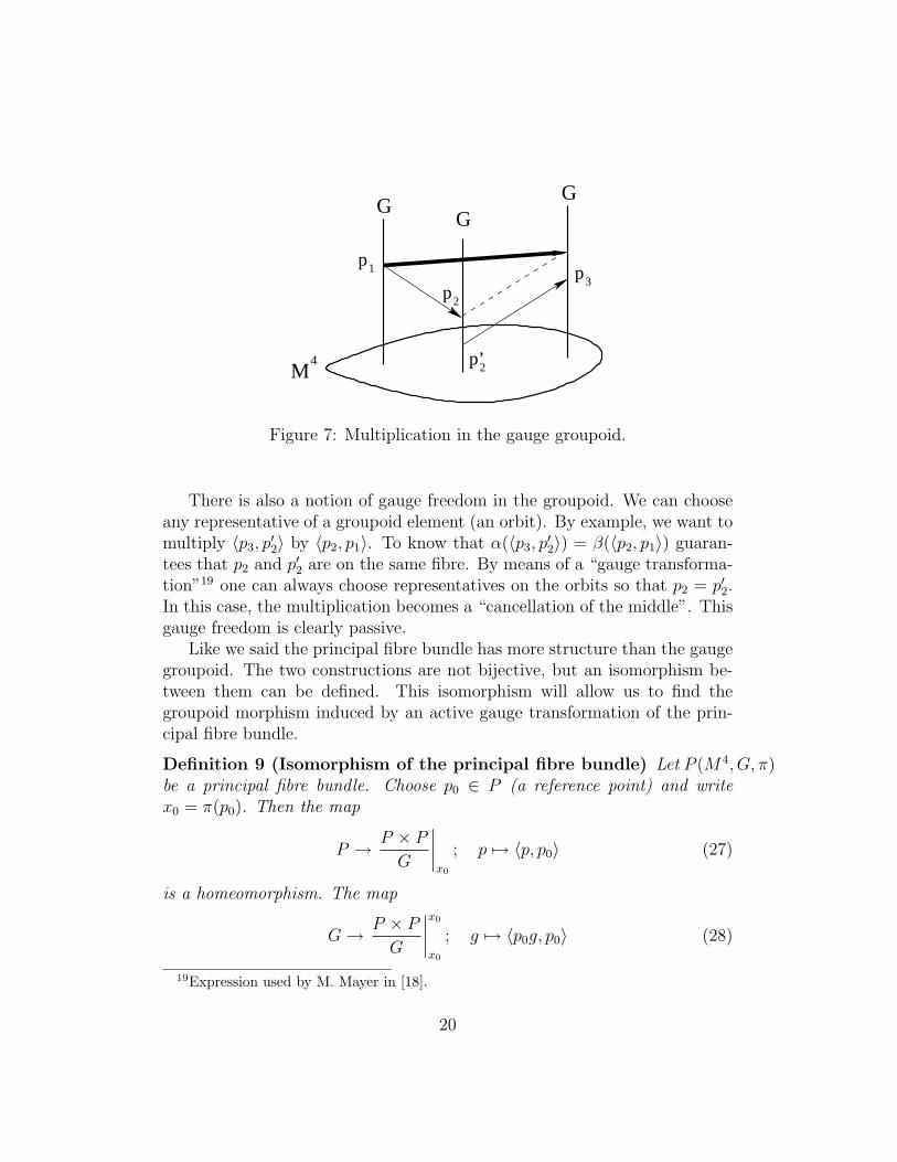
Figure 7: Multiplication in the gauge groupoid.

There is also a notion of gauge freedom in the groupoid. We can chooseany representative of a groupoid element (an orbit). By example, we want tomultiply 〈p3, p

′2〉 by 〈p2, p1〉. To know that α(〈p3, p

′2〉) = β(〈p2, p1〉) guaran-

tees that p2 and p′2 are on the same fibre. By means of a “gauge transforma-tion”19 one can always choose representatives on the orbits so that p2 = p′2.In this case, the multiplication becomes a “cancellation of the middle”. Thisgauge freedom is clearly passive.

Like we said the principal fibre bundle has more structure than the gaugegroupoid. The two constructions are not bijective, but an isomorphism be-tween them can be defined. This isomorphism will allow us to find thegroupoid morphism induced by an active gauge transformation of the prin-cipal fibre bundle.

Definition 9 (Isomorphism of the principal fibre bundle) Let P (M4, G, π)be a principal fibre bundle. Choose p0 ∈ P (a reference point) and writex0 = π(p0). Then the map

P → P × P

G

∣∣∣∣x0

; p 7→ 〈p, p0〉 (27)

is a homeomorphism. The map

G→ P × P

G

∣∣∣∣x0

x0

; g 7→ 〈p0g, p0〉 (28)

19Expression used by M. Mayer in [18].

20

is an isomorphism of topological gauge groups. Together they form an iso-morphism between the principal bundle and the gauge groupoid.

Thus the way to relate principal bundle to gauge groupoid is by the meansof one or more reference points. This dependance made Kirill Mackenzieasserts that if a phenomenon on a principal fibre bundle is formulated ingroupoid terms then it will be an intrinsic concept, independant of referencepoints (page 30, [14]). The gauge groupoid is describing the intrinsic relationsbetween properties at different space-time points. This is all we need inquantum mechanics. The introduction of a charge space was inspired bythe way we represent degrees of freedom in space-time. Since internal space(charge space) and space-time could be of totally different nature, it is notnecessary to use the same geometrical mean to represent them.

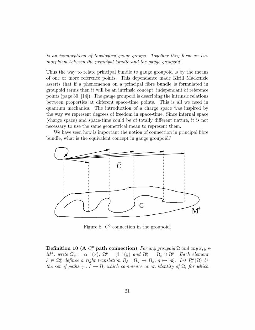
We have seen how is important the notion of connection in principal fibrebundle, what is the equivalent concept in gauge groupoid?

−

MC 4

C

Figure 8: C0 connection in the groupoid.

Definition 10 (A C0 path connection) For any groupoid Ω and any x, y ∈M4, write Ωx = α−1(x), Ωy = β−1(y) and Ωy

x = Ωx ∩ Ωy. Each elementξ ∈ Ωy

x defines a right translation Rξ : Ωy → Ωx; η 7→ ηξ. Let Pα0 (Ω) be

the set of paths γ : I → Ω, which commence at an identity of Ω, for which

21

α γ : I → M4 is constant, where I = [0, 1]. A C0 connection20 in Ω is amap Γ : C(I,M4) → Pα

0 (Ω); c 7→ c, satisfying the following conditions:

1. c(0) = c(0) and β c = c

2. If ϕ : [0, 1] → [a, b] ⊆ [0, 1] is a homeomorphism then c ϕ = Rc(ϕ(0))−1(c ϕ).

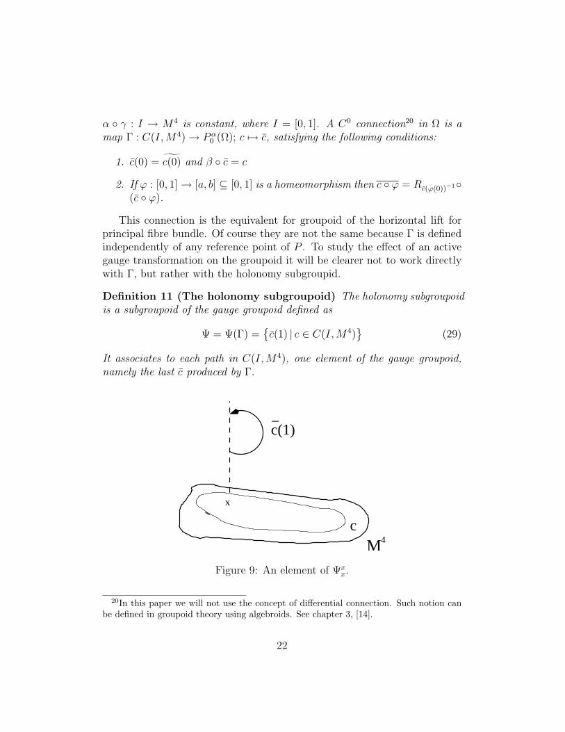
This connection is the equivalent for groupoid of the horizontal lift forprincipal fibre bundle. Of course they are not the same because Γ is definedindependently of any reference point of P . To study the effect of an activegauge transformation on the groupoid it will be clearer not to work directlywith Γ, but rather with the holonomy subgroupid.

Definition 11 (The holonomy subgroupoid) The holonomy subgroupoidis a subgroupoid of the gauge groupoid defined as

Ψ = Ψ(Γ) =c(1) | c ∈ C(I,M4)

(29)

It associates to each path in C(I,M4), one element of the gauge groupoid,namely the last c produced by Γ.

x

Mc

c(1)−

4

Figure 9: An element of Ψxx.

20In this paper we will not use the concept of differential connection. Such notion canbe defined in groupoid theory using algebroids. See chapter 3, [14].

22

Holonomy subgroupoid or holonomy groupoid is a very rich concept. If werestrict C(I,M4) only to path finishing at the same point they have begun,we obtain Ψx

x, the holonomy groups in principal bundle, in other words thesubgroup of G that can be related by a parallel transport on a closed path.For more details see the book of Lichnerowicz [12]. Add to Ψx0 a referencepoint p0 such that π(p0) = x0 and we otain the holonomy bundle of P (M4, G)through p0, in other words all points that can be parallel transported fromp0. Ψ clearly represent the intrinsic topological structure generated by theEhresmann connection ω.

We have seen that to an active gauge transformation corresponds a ver-tical automorphism R of the principal fibre bundle. Using the principalbundle isomorphism, it is easy to define the associated groupoid morphismR. If we apply this morphism to the holonomy groupoid we note that ingeneral Ψ′ = R(Ψ) 6= Ψ. However, we can also note a very interesting fact.For any vertical automorphism R and for all x ∈M4 then R(Ψx

x) = Ψxx. This

fact will be very important in the next subsection.

3.3.2 The gauge symmetry in nonrelativistic quantum mechanics

One of the difficulties to apply geometrical ideas to quantum mechanics isthat the phase space in such a theory is based on a noncommutative alge-bra. This fact seems to imply that this theory could not be represented bya geometry of points. One possibility to bypass this difficulty is to work inthe frame Alain Connes noncommutative geometry [5]. This is maybe themore natural path, but it is not what we will do here. There is a way toget philosophical insights about gauge symmetry without using the full arse-nal of noncommutative geometry. As quantization method, we will use theFeynman path integral (first developed in [9]). This approach of quantummechanics and quantum field theory has rarely been used in philosophicaldiscussions. However it is a reconstruction of quantum theory that is per-fectly legitimate. It is generally admitted that this so-called space-time orfunctional approach is completely equivalent to the standard Hamiltonianquantization methods, but for our purpose the advantage of the Feynmanformulation is that quantities involved in calculations remain classic. In thiscontext, our geometrical construction could still be used.

Let us begin with the simplest case: quantized particles under the influ-ence of a classical electromagnetic field. In that model, the path integral isdefined as

23

Definition 12 (Path integral) The probability amplitude (also called prop-agator), that a particle that was at the position ~q at time t = 0, is at position~p at time t = T , is

K(~p, T ; ~q, 0) =

∫D(~q(t)) e

i~ S[~q(t)] (30)

where S[~q(t)] is the classical action of the path ~q(t); in other words S[~q(t)] =∫ T

0L(~q, ~q) dt, where L(~q, ~q) is the Lagrangian of the particle. The integral∫D(~q(t)) is a sum over all possible trajectories between x = (0, ~q) and y =

(T, ~p).

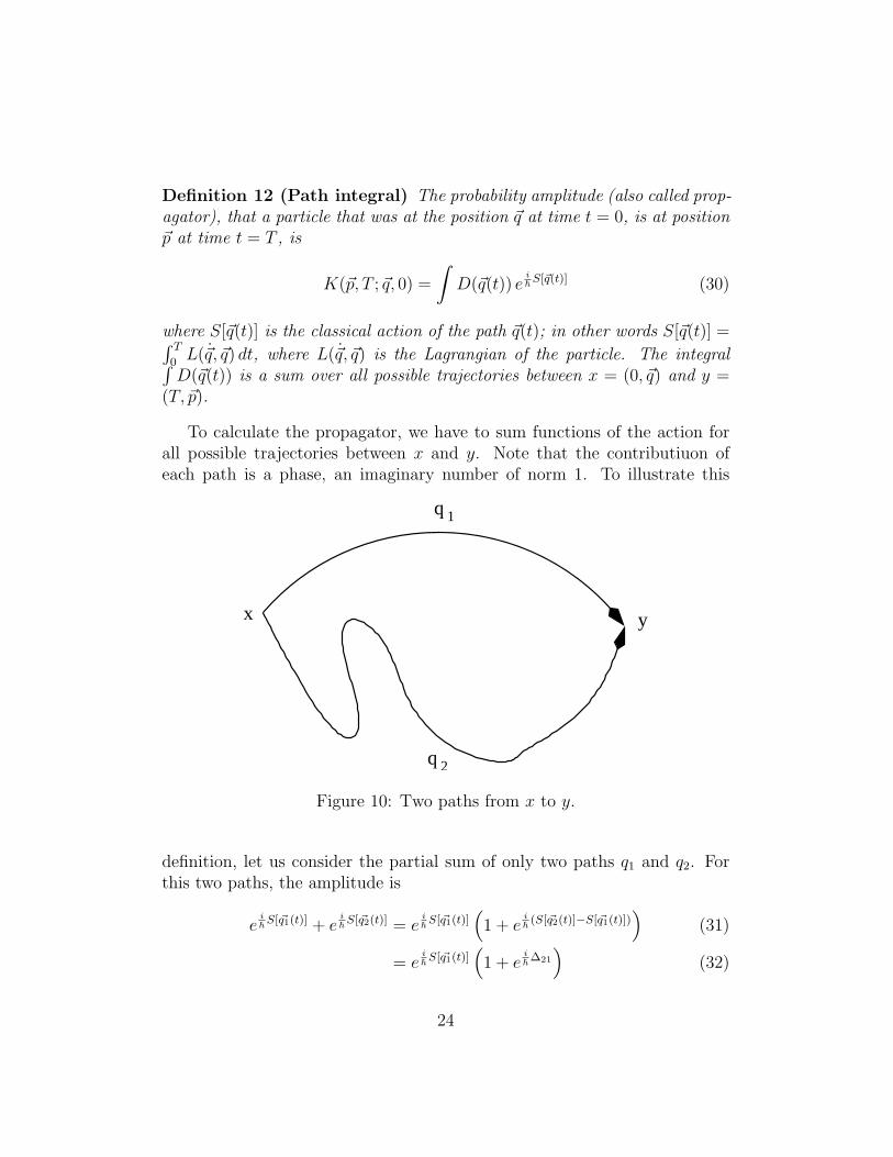
To calculate the propagator, we have to sum functions of the action forall possible trajectories between x and y. Note that the contributiuon ofeach path is a phase, an imaginary number of norm 1. To illustrate this

2

x y

q

q

1

Figure 10: Two paths from x to y.

definition, let us consider the partial sum of only two paths q1 and q2. Forthis two paths, the amplitude is

ei~ S[~q1(t)] + e

i~ S[~q2(t)] = e

i~ S[~q1(t)]

(1 + e

i~ (S[~q2(t)]−S[~q1(t)])

)(31)

= ei~ S[~q1(t)]

(1 + e

i~ ∆21

)(32)

24

We note that the relative phase between these two contributions ∆21 is theaction difference between the two paths. Since absolute phase is not mea-surable in quantum mechanics, if we had only these two paths to sum, onlythis relative phase would have a physical meaning.

What is the specific effect of electromagnetism on this particle? Classi-cally we know that if we add an electromagnetic interaction, the Lagrangianof the charged particle (of charge e) becomes:

L(~q, ~q) → L(~q, ~q) + e

(~v(t)

c· ~A(~q(t))− φ(~q(t))

)(33)

where ~v(t) is the velocity of the particle21. And the contribution to the pathintegral is modified in the following way:

exp

[i

~S[~q(t)]

]→ exp

[i

~

(S[~q(t)] + e

∫ (~v(t)

c· ~A(~q(t))− φ(~q(t))

)dt

)](34)

= exp

[i

~S[~q(t)]

]· exp

[ie

c~

∫ (d~q

dt· ~A− cφ

)dt

](35)

= exp

[i

~S[~q(t)]

]· exp

[− ie

c~

∫q

Aµdxµ

](36)

What the electromagnetic interaction does to the contribution of the path isto multiply it by a factor that depends only of the net parallel transport inthe principal fibre bundle over ~q between x and y. This factor is a phase thatdepends in general of the particular ~q. This model clearly points to considerelectromagnetism as a nonintegrable phase factor (see this position in Yang[29]). As we have seen in the last subsection, to the

∫qAµdx

µ correspondsan element of Ψy

x. By induction, we can see that the set Ψyx contains all

the information that we need to calculate the effect of an electromagneticinteraction on the propagator of a particle.

As we said, absolute phase is not measurable, only relative phase between

21For this discussion we will neglect the effect of the spin.

25

paths is. The effect of electromagnetism on ∆21 is

∆21 →∆21 −e

c

(∫q2

Aµdxµ −

∫q1

Aµdxµ

)(37)

= ∆21 −e

c

(∫q2

Aµdxµ +

∫−q1

Aµdxµ

)(38)

= ∆21 −e

c

∮Aµdx

µ (39)

From this result we can see that what is physically pertinent22 is not directlyΨy

x, but gauge groupoid elements such as ξη ∈ Ψxx, where η ∈ Ψy

x and ξ ∈Ψx

y . Holonomy groups are the only part of our geometrical construction(the structure express by the connection) that is physically significant innonrelativistic quantum mechanics. This is an important point. We arenot saying that the connection structure could be reformulate in terms ofholonomy groups. What we are defending is stronger than this mathematicalclaim. In the space-time approach of quantum mechanics, if we take inaccount the phase symmetry, Ψx

x is the only needed geometrical structureto express electromagnetic interaction. This observation could lead us tobelieve that quantum interaction is based on nonlocal properties (in the caseof Healy’s interpretation [11] on nonseparable properties). This conclusionwill not be defended here. Many ontological interpretations could fit thesame mathematical structure. Symmetries are more stable than ontologies.Thus I will concentrate my analysis on the symmetry status, leaving theontological problem open.

This result has an interesting effect on the interpretation of gauge sym-metry. Let us define the closed loop in space-time q = q1 + q2, let us writeΨ(q) = q(1) the element of the holonomy groupoid corresponding to thepath q, then

Ψ(q) = Ψ(q2)Ψ(q1) = Ψ′(q2)Ψ′(q1) = Ψ′(q) (40)

where Ψ′ = R(Ψ) is the holonomy groupoid after an active gauge trans-formation. In that case, the active gauge symmetry express a flexibility inthe choice of local relational properties compatible with a nonlocal structurerepresented by holonomy groups. Gauge symmetry is a surplus of structurecaused by the fact that we represent locally nonlocal relations.

22Remember we can factorize the contribution of q1 from the contribution of every paths.

26

This interpretation of gauge symmetry solves our puzzling question. Re-member the question was how gauge symmetry could be the result of a sur-plus of structure and in the same time not be arbitrary. This interpretationgives us an explanation. In the light of the Feynman approach of quantummechanics, the gauge symmetry is a surplus of structure. It is a symmetryof the Lagrangian that has no empirical consequence. On the other hand,subset Ψx

x of the holonomy groupoid have measurable effect. They have evena direct empirical effect in interference experiments, like the Aharonov-Bohmeffect.23 We saw that Ψx

x are gauge invariant. It seems reasonable to inter-pret gauge symmetry as a flexibility in the representation of Ψx

x. Since thisflexibility appears in an intrinsic geometrical context, it is not a case of co-ordinates change. It is rather a flexibility in the choice of a local connectioncompatible with holonomy groups. The gauge symmetry is not arbitrary.It is a consequence of the fact we have a choice of local constructions thatrepresent nonlocal geometrical structure.

Our work can easily be extended to nonabelien gauge interaction. Inthese cases, the phase factor (or Wilson line) will be

Uc(y, x) = Pe

igc~

R 10 ds dxµ

dsAa

µ(x(s))ta, (41)

where P is a prescription called path-ordering. This prescription takes inaccount the fact that Aa

µta matrices do not necessarily commute at different

points. For a closed path gauge invariant phase factor (called Wilson loop),we have to take the trace of Uc(x, x). The interpretation of gauge symmetryis the same than in the electromagnetic case.

3.4 Interpretation: relativistic quantum mechanics

For now we do not have a solid geometrical construction that we can applyto a fully quantized Yang-Mills theory. Thus the results of the precedingsubsection cannot directly be transfered to relativistic quantum mechanics.Let us examine briefly what is the main difficulty.

If we introduce a dynamical gauge potential, the path integral becomesnot well defined. ∫

D(A)ei~ S[A] (42)

23See MacKenzie [15] for a treatment of the Aharonov-Bohm effect using path integrals.

27

We have to sum on all possible configurations of the gauge potential. In doingso, we will count an infinite number of equivalent Aµ that differ only to agauge transformation. If we fix the gauge to solve this problem, we loose theunitarity of the theory and create unphysical states. The standard solutionis to introduce new terms in the Lagrangian; terms that include new fields,the Faddeev-Popov ghost fields. Therefore we add a surplus of structure tocompensate for another surplus of structure generated by gauge freedom. Itis not clear how geometry enters in this picture. Should we include a secondassociated vector bundle to accommodate ghost fields? What will be thegain in understanding?

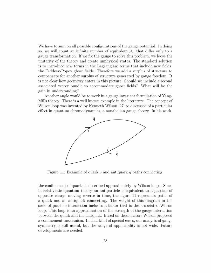
Another angle would be to work in a gauge invariant formulation of Yang-Mills theory. There is a well known example in the literature. The concept ofWilson loop was invented by Kenneth Wilson [27] to discussed of a particulareffect in quantum chromodynamics, a nonabelian gauge theory. In his work,

q

q_

Figure 11: Example of quark q and antiquark q paths connecting.

the confinement of quarks is described approximately by Wilson loops. Sincein relativistic quantum theory an antiparticle is equivalent to a particle ofopposite charge moving reverse in time, the figure 11 represents paths ofa quark and an antiquark connecting. The weight of this diagram in theserie of possible interaction includes a factor that is the associated Wilsonloop. This loop is an approximation of the strength of the gauge interactionbetween the quark and the antiquak. Based on these factors Wilson proposeda confinement mechanism. In that kind of special cases, our analysis of gaugesymmetry is still useful, but the range of applicability is not wide. Futuredevelopments are needed.

28

After Wilson more general quantum loop formulation were proposed. SeeGambini and Pullin [10] on the subject. But we are far from a sufficientlydeveloped theory to do philosophical analysis. The interpretation of gaugesymmetry is still an open problem in this context.

4 Conclusion

In this paper we push the geometrical interpretation of gauge symmetryas far as we could. We obtain a result in the context of nonrelativisticquantum mechanics. The gauge symmetry denotes there a flexibility in thelocal representation of nonlocal features of the interaction. The question ofthe interpretation of gauge symmetry for quantum field theory is still open.

References

[1] Y. Aharonov and D. Bohm. Significance of electromagnetic potentialsin the quantum theory. Physical Review, 115(3):485–491, August 1959.

[2] Michael Atiyah. Geometry of Yang-Mills fields. In Michael Atiyah Col-lected Works: gauge theories, volume 5, pages 75–173. Oxford UniversityPress, 1988.

[3] Gordon Belot. Understanding electromagnetism. The British Journalfor the Philosophy of Science, 49:531–555, 1998.

[4] Yvonne Choquet-Bruhat, Cecile DeWitt-Morette, and Margaret Dillard-Bleick. Analysis, Manifolds and Physics: Part 1. Elsevier, revised edi-tion, 1982.

[5] Alain Connes. Noncommutative Geometry. Academic Press, 1994.

[6] M. Daniel and C.M. Viallet. The geometrical setting of gauge theo-ries of the Yang-Mills type. Reviews of Modern Physics, 52(1):175–197,January 1980.

[7] P.A.M. Dirac. Quantised singularities in the electromagnetic field. Pro-ceeding of the Royal Society of London, Series A, 133(81):60–72, Septem-ber 1931.

29

[8] L.D. Faddeev and A.A. Slavnov. Gauge Fields: an introduction to quan-tum theory. Addison-Wesley Publishing Company, 1991.

[9] Richard P. Feynman. Space-time approach to non-relativistic quantummechanics. Review of Modern Physics, 20(2):367–387, April 1948.

[10] Rodolfo Gambini and Jorge Pullin. Lopps, Knots, Gauge Theories andQuantum Gravity. Cambridge University Press, 1996.

[11] Richard Healey. On the reality of gauge potentials. Philosophy of Sci-ence, 68(4):432–455, December 2001.

[12] Andre Lichnerowicz. Theorie globale des connexions et des groupesd’holonomie. Edizioni Cremonese, Roma, 1955.

[13] Holger Lyre. The principles of gauging. Philosophy of Science,68(3):S371–S381, September 2001. Proceedings of the 2000 BiennialMeeting of the Philosophy of Science Association.

[14] Kirill MacKenzie. Lie Groupoids and Lie Algebroids in Differential Ge-ometry. Cambridge University Press, 1987.

[15] Richard MacKenzie. Path integral methods and applications. arXiv:quant-ph/0004090, April 2000.

[16] Christopher A. Martin. Gauging Gauge: On the Conceptual Foundationsof Gauge Symmetry. PhD thesis, University of Pittsburgh, 2002.

[17] Meinhard E. Mayer. Groupoids and Lie bigebras in gauge and stringtheories. In K. Bleuler and M. Werner, editors, Differential Geomet-rical Methods in Theoretical Physics, pages 149–164. Kluwer AcademicPublishers, 1988.

[18] Meinhard E. Mayer. Principal bundles versus lie groupoids in gaugetheory. In L.-L. Chau and W. Nahm, editors, Differential GeometricMethods in Theoretical Physics, pages 793–802. Plenum Press, 1990.

[19] John McCleary. A history of manifolds and fibre spaces: tortoises andhares. To be published in Supplemento ai Rendiconti del Circolo Matem-atico di Palermo.

30

[20] Lochlainn O’Raifeartaigh. The Dawning of Gauge Theory. PrincetonUniversity Press, 1997.

[21] Michael Redhead. The interpretation of gauge symmetry. In MeinhardKuhlmann, Holger Lyre, and Andrew Wayne, editors, Ontological As-pects of Quantum Field Theory, pages 281–301. World Scientific, 2002.

[22] Joe Rosen. Fundamental manifestations of symmetry in physics. Foun-dations of Physics, 20(3):283–307, 1990.

[23] Paul Teller. The gauge argument. Philosophy of Science, Supplementto Volume 67(3):S466–S481, 2000.

[24] A. Trautman. Fibre bundles associated with space-time. Report onMathematical Physics, 1(1):29–62, 1970.

[25] Alan Weinstein. Groupoids: unifying internal and external symme-try. Notices of the American Mathematical Society, 43(7):744–752, July1996.

[26] Eugene P. Wigner. Symmetry and conservation laws. In PhilosophicalReflections and Syntheses, pages 297–310. Springer, 1995.

[27] Kenneth G. Wilson. Confinement of quarks. Physical Review D,10(8):2445–2459, October 1974.

[28] Tai Tsun Wu and Chen Ning Yang. Concept of nonintegrable phasefactors and global formulation of gauge fields. Physical Review D,12(12):3845–3857, December 1975.

[29] C.N. Yang. Integral formalism for gauge fields. Physical Review Letters,33(7):445–447, August 1974.

31