arX

iv:0

710.

2872

v1 [

astr

o-ph

] 15

Oct

200

7

Geometrical constraints on dark energy modelsRuth Lazkoz

Fisika Teorikoa, Euskal Herriko Unibertsitatea, 644 postakutxatila, 48007 Bilbao, España

Abstract. This contribution intends to give a pedagogical introduction to the topic of dark energy(the mysterious agent supposed to drive the observed late time acceleration of the Universe) andto various observational tests which require only assumptions on the geometry of the Universe.Those tests are the supernovae luminosity, the CMB shift, the direct Hubble data, and the baryonacoustic oscillations test. An historical overview of Cosmology is followed by some generalities onFRW spacetimes (the best large-scale description of the Universe), and then the test themselves arediscussed. A convenient section on statistical inference is included as well.

Keywords: dark energy, observational testsPACS: 98.80.Es, 04.50.+h

INTRODUCTION

Cosmology is a branch of physics which is experiencing a tremendously fast devel-opment lately triggered by the arrival of many new observational data of ever moreexquisite precision. These findings have been crucial for the improvement in our under-standing of the Universe, but the vast amount of knowledge onour Cosmos which wehave nowadays would never have been possible without the concerted effort by exper-imentalists and theoreticians. One of the results of this fantastic intellectual pursue isthe puzzling discovery that there is in the Universe a manifestation of the repulsive sideof gravity. This is the topic to which this lectures are devoted, and more specifically Iwish to address some methods which the community believes are useful for building adeeper understanding of why, how and when our universe beganto accelerate. Put inmore modest words, these lectures will dissert about how onecan take advantage ofvarious observational datasets to describe some basic features of the geometry of theUniverse with the hope they will reveal us something on the nature of the agent causingthe observed accelerated expansion.

As this is quite an advanced topic in Physics (Astronomy), this contribution will buildtougher as we proceed, so I hope the readers will enjoy to start off from a little historicstroll in the science of surveying the skies. For wider historical overviews than the onepresented here, the two main sources I recommend to you, among the so many available,are [1] and [2].

Historical records tells us that Astronomy was born basically because of the need byagrarian societies to predict seasons and other yearly events and by the esoteric needto place humanity in the Universe. This discipline developed in many ancient cultures(Egyptian, Chinese, Babylonian, Mayan), but it was only Greek people who cared un-derstanding their observations and spreading their knowledge unlike in other cultures.Their influence was crucial as the modern scientific attitudeof relying in empiricism(Aristotlean school) and translating physical phenomena into the mathematical language

(Pithagorean school) built on their way of approaching science. Unfortunately, Aristo-tle was far so influential that his erroneous geocentric viewof the Universe was notquestioned aloud until the XVIth century.

At the beginning of that century Copernicus started to spread quietly his heliocentriccosmological model, and even though he did not make much propaganda about his ideas,they deeply influenced other figures, such as Galileo, who introduced telescopes into as-tronomy and found solid evidence against the geocentric model. Another very importantcontribution to the subject was made by Kepler, who gave accurate characterization ofthe motions of the planets around the Sun. These findings werelater on syntheticallyexplained by Newton in his theory of gravitation, which built on Galileo’s developmentson dynamics (the law of inertia basically).

The XVIIIth and XIXth century brought advances in the understanding of the Uni-verse as a whole made of many parts which lie not necessarily in the Solar system. Starsbegan to be regarded as far-away objects in motion, and otherobjects like nebulae werediscovered, so the idea of the existence of complicated structures outside the Solar sys-tem gained solidity. A discovery very much related to the main topic of this lectures wasthe realization that the combination of the apparent brightness of a star and its distanceget combined to give its intrinsic brightness; basically the amount of energy reachingus in the form of light from a distant source decreases is inversely proportional to thesquare of the distance between the source an us (in an expanding the universe definitionof distance is not the same as in a static one but this broad wayof speaking applies allthe same) This finding let observers realize that stars were objects very much like theSun, or if you prefer they realized the Sun was nothing but yetanother star.

The most important next breakthrough was Einstein’s theoryof special relativity,which generalized Galileo’s relativity to introduce light. On the conceptual realm, thiswas a very revolutionary theory at is warps the notions of space and time, and so it set thefoundations for the best description of gravity so far: Einstein’s theory of General Rela-tivity. This second theory was the fruition of Einstein endeavors to unify the interactionsknown to him. In this theoretical framework matter/energy modifies the geometry, andin turn geometry tells matter/energy how to move/propagate(paraphrasing Wheeler’srenowned quotation). Among other predictions this theory made a couple which arecornerstones of modern astronomy: gravitational redshift(light gets redder as it movesaway from massive objects), and gravitational lensing (light gets bent as it passes closeto massive objects).

The next important advance come from the side of observations. In 1929 Hubble,and after having collected data carefully for almost a decade, presented the surprisingconclusions that galaxies on average move away from us. Thiseffect is encoded in thescale-invariant relation known as Hubble’s law:v= Hd, wherev is the galaxy’s velocityandd its distance from us. The positiveness of the quantityH as measured by Hubbleis precisely what told him the Universe is expanding, this being a discovery which getsaccommodated nicely in Einstein’s theory of general relativity. Interestingly, on learningabout this finding, Einstein discarded his idea of the necessity of some exotic fluid withnegative pressure to counteract the attractive effect of usual matter (which would makethe universe contract). It cannot look but funny from today’s perspective that Einstein’sidea has come to life again, at the end of the day the exotic fluid he imagined is one ofthe possible flavors of what the community calls dark energy [3] these days.

At the risk of not giving everyone the credit they merit, I will just say that recog-nition for the concept of a expanding Universe is due to both theoreticians (de Sitter,Friedmann, Lemaître, Gamow,...) and experimentalists (Slipher, Hubble,..). However,the trampolin for this idea to jump into orthodoxy was put by Penzias and Wilson [4]who first detected the cosmic microwave background, and by Dicke, Peebles, Roll andWilkinson [5] who were responsible for the not the less important interpretation of thoseobservations. The existence of this radiation and its characteristic black body spectrumare a prediction of the Big-Bang theory, it is fair to say thatif one combines it with othersources of evidence, it is almost impossible to refute it.

The CMB in an invaluable source of cosmological information(visit [7] for a higlyrecommended site on the subject). It has a temperature of of around 2.73K, with tinytemperature differences of about 10−5 between different patches of the sky. Theseanisotropies inform us that the photons forming the CMB where subject to an underlyinggravitational potential which had fluctuations, and this isjust and indication of densityirregularities that seeded the structure one observes today. On the other hand, the imageof the features of the CMB in different angular scales strongly favors a universe with nospatial curvature (flat or Euclidean on constant time slices) that is, it supports the theoryof inflation. In addition, the CMB has a saying about the fraction of the different fluidsfilling the Universe.

Fortunately, the mine of cosmic surprises was far from beingexhausted, and it storeda diamond of many carats in the form of a discovery which has changed greatly themainstream view of the Universe. Up to the late 1990, no repulsive manifestationof gravity had been spotted in Nature. In 1998 astronomical measurements providedevidence that gravity can not only push, but pull as well, andthe repulsive side of gravitygot unveiled. Very refined observations of the brightness ofdistant supernovae [8, 9]seemed to hint the presence of a negative pressure componentin the Universe whichwould make it accelerate, and then a new revolution started.

One may wonder at this stage what is the relation of supernovae luminosity and cos-mic speed up. Objects in the Universe with a well calibrated intrinsic luminosity (super-novae, for instance) can be used to determine distances on cosmological scales. Super-novae are very bright objects, and so they result particularly attractive for this purpose(they can be 109 times more luminous than the Sun so there is hope they will be visiblefrom up to perhaps 1000 Mpc [10]). As we anticipated in the last paragraph, in 1998 twoindependent teams reported evidence that some distant supernovae were fainted than ex-pected. This involved tracing the expansion history of the Universe by combining mea-surements of the recession velocity, apparent brightness and distance estimations. Themost compelling explanation was (and keeps being as far I am concerned) that their lighthad traveled greater distances than assumed. The orthodox view up to then was that theexpansion pace of the Universe was barely constant, but supernovae seemed to contra-dict this. This unexpected and exciting discovery obliged researchers to broaden theirmind and accept the Universe is undergoing accelerated expansion.

I should have been able to have convinced the readers by now that these are excitingtimes to be working on Cosmology, as cosmic speed up is such and intriguing phe-nomenon with major open questions such as whether dark energy evolves with time,how much of it is there, and if is rather not a manifestation ofextradimensional physics.

The answer to these questions requires cannot be dissociated from the response to aperhaps more fundamental question: what is the Universe made of?

The combination of various astronomical observations tellus our universe is basicallymade of thee major components (see for instance [11]). The most abundant one is darkenergy [3], so this makes it even more interesting to find out whatever we can aboutit. At the other end the by far least abundant component is baryonic matter, and in themiddle (as abundance is concerned) we have dark matter, in a proportion comparable tothat of dark energy. There are various sources of astrophysical giving evidence in favorof it. Hints of it is existence are provided by the motion of stars, galaxies and clusters,but it is known it also played a crucial role in the amplification of the primordial densityfluctuations which seeded the large scales structure we observe today and dark matterimprints can be found in the CMB as well. Dark matter represents quite a challengeas its nature remains a mystery; nevertheless if it were baryonic we know from bigbang nucleosynthesis helium-4 would get converted to deuterium much easily and CMBcalculations indicate indicate in addition anisotropies would be much larger so the oddsare most of its is not baryonic.

Up to here we have made a very broad introduction to our topic with a little bit ofhistory and a little bit of physics, but we must not forget Maths are key to Cosmology[12]. We only know how to study the Universe using numbers andequations, butof course progress in this direction is done with as many reasonable simplificationsas possible (if they do not compromise rigor, of course). Einstein equations relategeometry and matter/energy content of the Universe. Cosmologists are concerned bythis relation on a large scales picture so as to understand the expansion of the Universe.Those equations are non-linear, so studying them is painstaking unless one exploits theobservational evidence the regularity of the Universe. Non-linearity of those equationsmakes their study a really hard task so simplifications are a must. The two basic ones arethat galaxies are homogeneously distributed on galaxies larger than 50 Mpc [13], andthat the Universe is isotropic around us on angular scales larger than about 10 degrees[14]. But this is not enough, those two simplifications, which come from observationalevidence must be completed with the assumption we occupy no special place in theUniverse.

This puts on the track of what we could call the parameterizedUniverse, cosmologistswork with a greatly a simplified geometric description of theUniverse which emergesfrom the latter assumptions. The models for the sources are of reduced complexity too,the most common being perfect fluids and fields with known dynamics. This we haveon the side of theory, but on the side of observations we have to make our own lifeeasier too. When doing observations oriented Cosmology, one uses as a variable theredshiftz of the electromagnetic radiation received, as it encodes information of howmuch the Universe has expanded between emission and reception. Observational tablesof geometrical quantities can be given, and then one can testdifferent theoretical valuesof the same quantities corresponding to models of interest.The theoretical predictionswill depend on the sources assumed, and ultimately it will bepossible to estimate thesuitability of a given dark energy model to observations, but which are the availableprobes of dark energy?

Basically dark energy can be scrutinized observationally from two main perspectives[15]: one possility is doing it through its effect of the growth of structures, another

one is through its impact on geometrical quantities. We willconcentrate on geometricalconstraints/tests in these lectures as in a way they are those which can perhaps be appliedwith less difficulty, although their simplicity does not mean they are the least interesting,for instance, the supernovae test is the only test giving a direct indication of the need ofa repulsive component in the Universe, whereas the baryon acoustic oscillations test isthought to have much information in store. Discussion on these two tests will be givenlater on in these lectures.

Finally, there is one more direction in which these topic is related to Maths apart fromthe geometrical side of it, statistics plays an important role too. Physics is attractivebecause of its ability to “tame” natural phenomena in the sense that laws of physics bringorder to the apparent chaos of Nature, Astrophysics is even more attractive because itevidences how laws of physics apply outside Earth, which is certainly surprising giventhe manifest differences between Earth and every other locations in the Universe ofwhich we are aware. However, since these phenomena occur in places far, far away, andsometimes they can only be observed indirectly, there is typically an important degreeof uncertainty. Thus, research is Astrophysics requires understanding not only Physics,but also inference.

Inferential statistics cares for the identification of patterns in the data taking in accountthe randomness and uncertainties in the observations. In contrast, descriptive statisticsis concerned with giving a summary of the data either numerically or graphically. Bothwill be needed toward two goals: we need to know optimal ways to extract informationfrom the astronomical data, but we also need to know rigorousapproaches to comparetheoretical predictions to observations.

Our approach will be that of Bayesian inference, and we will justify jut below mypreference, but it must be admitted there is an old vivid controversy on the definition ofprobability between the two main schools: frequentists andBayesians. Frequentists usea definition based on the possibility of repeating the experiment, but this does not applyto the Universe, and this sounds like the reason why the number of Bayesian astronomersgrows every day, but you should not care for this battle rightnow; just stick to the ideathat observations related Cosmology needs to resort to Statistics and that Inference isvital for constraining dark energy cosmological models.

By now you should be able to guess what to expect in the next sections. I willpresent you some basics of FRW (Friedmann-Robertson-Walker) cosmologies, then Iwill devote a great deal of this text to details of geometrical tests, and leave for the lastbut one section a convenient primer on statistics.

GENERAL RELATIVITY AND FRW

Einstein’s influence in cosmology is paramount, Special Relativity is crucial in high en-ergy physics, which plays an important role in astronomy andcosmology, as many pro-cesses one studies in these areas are very energetic. But General Relativity is even moreimportant for Cosmology as it allows to describe the gravitational interaction, which isthe one governing the dynamics on planetary, galactic and cosmological scales. Gravityin astronomy is mostly treated classically as opposed to quantum mechanically, as nosuccessful theory of gravity exist. The situation is different with respect to Special Rela-

tivity, as the connection with the quantum realm is satisfactorily given by quantum fieldtheory. Given that Special Relativity is the conceptual precursor of General Relativity, afew lines about it are worth before entering an overview of General Relativity.

Part of the topics of this section are extensively covered in[16, 17, 18, 19].Special Relativity stands on two pillars. The first one is that the laws of physics are

the same in all inertial frames, reference systems in which bodies are not subject toforces remain at rest or in steady linear motion. The second one is that the speed oflight in vacuum,c, is the same in all inertial frames as confirmed by the Michelson-Morley experiment, but actually anticipated intuitively by Einstein. Inferring conclu-sions from those two premises requires treating the quantity ct on the same grounds asspatial coordinates (sayx,y,z), and this interchangeability of space and time make theconcept of spacetime emerge. When transforming between inertial frames, the quantityds2 = c2dt2−dx2−dy2−dz2 remains invariant,ds2 being the norm of the four-vector(cdt,dx,dy,dz).

Special Relativity requires the laws of physics to be written in terms of four-vectors astheir norms do not change on going from one inertial frame to another. The quantityds2

is called the line-element, and it quantifies the distance between events of the spacetime.The line-element is a quadratic form constructed from a matrix g: ds2 = gµνdxµdxν forµ,ν = 0,1,2,3 In Special Relativitygi j = diag(1,−1,1,1), but in General Relativity itneed not be diagonal nor constant.

This brief account on Special Relativity drives us into the theoretical ground ofGeneral Relativity. In developing this beautiful theory Einstein was influenced by fiveprinciples: Mach’s principle (geometry or motion do not make sense in an emptyuniverse);principle of equivalence (the laws of physics look the same to an observerin non-rotating free fall in a gravitational field and to an observer in uniform motion inthe absence of gravity),principle of general covariance (laws of physics must havethe same for all observers),correspondence principle (from General Relativity onemust recover on the one hand gravity Special Relativity whengravity is absent, and onemust also recover Newtonian gravity when gravitational fields are week and motions areslow, actually, this principle reflects the very reasonableneed that any new scientificframework must be consistent with precursor reliable frameworks in their range ofvalidity.)

According to records, walking the tortuous path from Spatial Relativity to GeneralRelativity took Einstein 11 years. Let us outline the main elements of the construction:gravity can be waived locally and regain Special Relativity, locally gravitational effectslook like any other inertial effect, test particles are assumed to travel on geodesics(null ones if they are photons and timelike ones if they are massive), inertial forcesare accounted for in the geodesic equations by terms which depend on first derivativesof the metric (which plays the role of the potentials of the theory), gravitational fieldsmake geodesics converge/diverge as described by some termsin the geodesic deviationequation which depend on the Riemann tensor (which depends on second derivativesof the metric), all forms of energy act as sources for the gravitational field and this isencoded in the Einstein equations.

In General Relativity tensors play a preeminent role. The Riemann tensor or curvaturetensorRa

bcd determines how geodesic deviates, and upon contraction it gives the curva-

ture or Ricci tensorRab= gcdRdacb. Further contractions allow deriving the curvature orRicci scalarR= gabRab, and finally, the connection between matter/energy and curvatureis encoded in the Einstein equations

Gab = 8πGTab/c4, (1)

whereGab = is the Einstein tensor andTab is the Einstein tensor.At this point we have now enough theoretical machinery to study the dynamics of a

standard universe, but I must insist on the fact that studying the Universe without mak-ing radical but reasonable simplifications would be a intractable problem. Fortunately,progress can be made because we are lucky enough to have evidence of its regularity.As already mentioned in the introduction, we have evidence on the one hand of the ho-mogeneity in the distribution of galaxies on scales larger than 50 Mpc [13], and on theone hand CMB experiments inform us on the isotropy around us on angular scales largerthan a 10 degrees [14]. If one then invokes that our place is the Universe is not special atall, then isotropy around all its points in inferred. Finally, there is a theorem in geometrywhich tells us that if every observer sees the same picture ofthe Universe when lookingat different directions, then the Universe is homogeneous.

These assumptions boil down into the (Friedmann-)Robertson-Walker metric. OurUniverse can be viewed as an expanding, isotropic and homogeneous spacetime, andthat means its line element reads

ds2 = c2dt2−R(t)2(dr2+S2(r)(dθ2+sin2(θ)dφ2), (2)

with R(t) an arbitrary andS(r) a function which can take three distinct forms. If onedefinesR(t)= a(t)R0, and then makesr → r/R0, a more familiar expression is obtained:

ds2 = c2dt2−a(t)2(dr2+S2(r)(dθ2+sin2(θ)dφ2)), (3)

wherea(t) is a dimensionless quantity (customarily chosen to have value 1 at present).The geometry of spatial sections in the FRW metric are also worth some further

discussion. The functionS(r) must be such the spatial sections of the RW geometry haveconstant curvature, so the possibilities areS(r) = sin(r), r,sinh(r). Again, a familiarform of the line-element is obtain by makingS(r)2dr2 → dr2/(1−kr2), and so the threecases are respectivelyk= 1,0,−1 (as shown in Fig. 1).

Before proceeding, a little remark is convenient. From hereon we will use the socalled natural units 8πG= c= 1 under otherwise stated. Having made this comment inpassing let us turn our attention to the right hand side of theEinstein equations, i.e to thematter/energy content.

We have seen that simplifications in geometry are required tomodel the Universe.In the same spirit reduction of sophistication in the description of matter/energy is alsorequired. Simplicity on the one hand, and consistency with observations in the other,suggest adopting the perfect fluid picture (no viscosity is assumed):

Tab = (ρ + p)uaub+ pgab, (4)

with ρ , p andua representing the energy density, pressure and velocity field of the fluid.Note that in the rest frame of the fluid

Tab = diag(ρ ,−p,−p− p). (5)

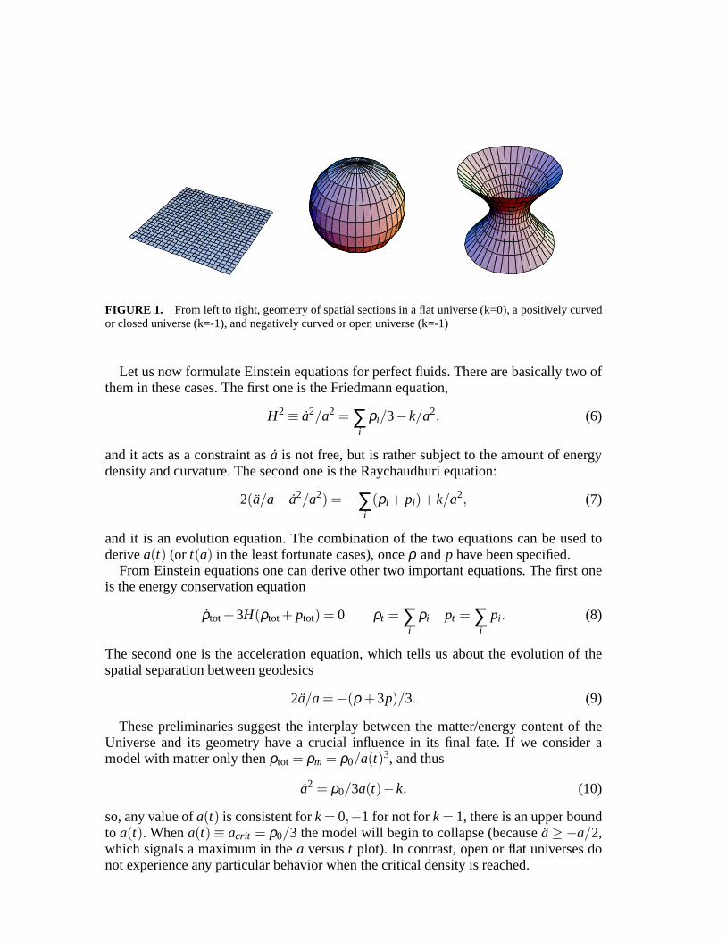
FIGURE 1. From left to right, geometry of spatial sections in a flat universe (k=0), a positively curvedor closed universe (k=-1), and negatively curved or open universe (k=-1)

Let us now formulate Einstein equations for perfect fluids. There are basically two ofthem in these cases. The first one is the Friedmann equation,

H2 ≡ a2/a2 = ∑i

ρi/3−k/a2, (6)

and it acts as a constraint as ˙a is not free, but is rather subject to the amount of energydensity and curvature. The second one is the Raychaudhuri equation:

2(a/a− a2/a2) =−∑i(ρi + pi)+k/a2, (7)

and it is an evolution equation. The combination of the two equations can be used toderivea(t) (or t(a) in the least fortunate cases), onceρ andp have been specified.

From Einstein equations one can derive other two important equations. The first oneis the energy conservation equation

ρtot+3H(ρtot+ ptot) = 0 ρt = ∑i

ρi pt = ∑i

pi . (8)

The second one is the acceleration equation, which tells us about the evolution of thespatial separation between geodesics

2a/a=−(ρ +3p)/3. (9)

These preliminaries suggest the interplay between the matter/energy content of theUniverse and its geometry have a crucial influence in its finalfate. If we consider amodel with matter only thenρtot = ρm = ρ0/a(t)3, and thus

a2 = ρ0/3a(t)−k, (10)

so, any value ofa(t) is consistent fork= 0,−1 for not fork= 1, there is an upper boundto a(t). Whena(t)≡ acrit = ρ0/3 the model will begin to collapse (because ¨a≥ −a/2,which signals a maximum in thea versust plot). In contrast, open or flat universes donot experience any particular behavior when the critical density is reached.

0 0.5 1 1.5 2 2.5 3Wm

0

0.5

1

1.5

2

2.5

WLno

big

bang

big

bang

expands forever

recollapses

acce

lera

ting

dece

lera

ting

closedopen

DΘ

P1

P2

P4

P3

Dz

z

(a) (b)

FIGURE 2. (a) Regions for the LCDM model. (b) A spherical shell in redshift space.

The addition of a cosmological constant brings a richer set of possibilities (see Fig.2(a)). It is convenient to present the cases using fractional densities:

Ωk =−k/H2a2, ΩΛ = Λ/3H2, Ωm = ρm/3H2, Ωm+ΩΛ +Ωk = 1. (11)

Let us consider now perfect fluid cosmological histories. Many p(ρ) equations of stateare considered in the literature, but the linear one,p= wρ , stars in popularity. Here youhave a list some physically meaningful cases in thek= 0 case.

• Electromagnetic radiation, i.e. photons,w= 1/3, ρ ∼ a−4, a(t)∼ t1/2

• (Incoherent) matter, aka cosmic dust,w= 0, ρ ∼ a−3, a(t)∼ t2/3

• Vacuum energy, aka cosmological constant,w=−1, ρ ∼ cons, a(t)∼ eHt

• Quiessence [20],w= cons<−1/3 6=−1, ρ ∼ a−3(1+w), a(t)∼ t2/(3(1+w))

There are, of course, more complicated equations of state that have received attentionin connection with late-time acceleration. A list (with some bias, as that of perfect fluids)can be this one:

• Conventional Chaplygin gas [21], p=−A/ρ , ρ ∼√

A+B/a6

• Generalized Chaplygin gas [22], p=−A/ρα , ρ ∼(

A+B/a3(1+α))1/(1+α)

• Inhomogeneous equation of state [23],p=−ρ −Aρα , ρ1−α ∼ A(1−α) loga

Last but not least, another very popular class of sources in Cosmology is that of scalarfields. Usually, they can be interpreted as perfect fluids, but the main difference is thatthe equation of state changes over time. Many scalar field models have been proposed(for the early and the late universe):

• quintessence [24],ρ = φ2/2+V(φ) p= φ2/2−V(φ)

• k-essence [25],ρ =V(φ)(

2φ2∂F(−φ2)/∂ φ2−F(−φ2)

)

p=V(φ)F(−φ2)

• tachyon [26],ρ =V(φ)/√

1− φ2 p=−V(φ)√

1− φ2

• quintom [27],ρ = (φ21 − φ2

2)/2+V(φ1,φ2) p= (φ21 − φ2

2)/2−V(φ1,φ2)

This schematic account of the possible types of matter/energy content in Cosmologydoes not make justice at all to the vast literature on the subject, but we must stop hereand return to geometric aspects.

Commonly, cosmological parameters are constrained by studying how distant lightsources are seen from our detection devices, and this depends on the cosmologicalmodel. In an expanding FRW model light gets redshifted during its trip from the sourceto the observer, and the redshift depends on the amount of expansion occurred mean-while:

a(tobs)/a(temit) = 1+z≡ λobs/λemit. (12)

As light travels along null geodesics, one can compute the redshift experienced by aphoton as it travels a given radial distance

dt2−a2dr2 = 0 impliesdr = dz/H(z), (13)

we have takena0 = 1 andc= 1 in dr = cdz/H(z) and the metric is the FRW one. Thoseare basic ingredients for the construction of “distances” in cosmology (see [28] for apedagogical acount of the topic).

Now, there is a basic concept we need so as to make progress in the topic of distancesin Cosmology: comoving coordinates. One of the niceties of General Relativity is itallows to formulate physical laws in whatever system of coordinates one may prefer.In Cosmology, those coordinates have become very popular because they make one’slife a lot easier. Observers which see the Universe as isotropic have constant values ofspatial coordinates when the comoving system is used. Non-comoving observers will seeredshifts in some directions and blueshifts in others, and the time measured by comovingobservers is cosmological time.

One of the quantities required for our geometrical tests is the line of sight comovingdistance. This is the comoving separation between two objects with the same angularlocation but different radial position (P1P2 in the picture). The comoving distance fromus to an object atz

DC =∫ z

0dz/H(z), (14)

whereas from the former we can derive that the comoving distance between two objectsseparated∆z is DC = ∆z/H(z). The comoving distance is the proper distance betweenthose objects divided by the ratio of the scale factor of the Universe at the epochs ofemission of reception.

Another relevant definition is that of (transverse) comoving distance and angulardiameter distance. The comoving distance between two objects located at the same radialposition but separated by and angle∆θ is DM∆θ (P3P4 in Fig. 2(b)) whereDM = S(r) isthe transverse comoving distance. Closely related to the former we have the widely usedangular diameter distanceDA. It is defined as the ratio of an object’s physical transversesize to its angular size (in radians):

DA = DM/1+z. (15)

Finally, let me present the luminosity distance which is thekey to the extraction ofinformation from supernovae data. Given a standard candle its bolometric (i.e. integrated

over all frequencies) emitting power right at the position of the source is called theluminosityL. The total bolometric power per unit area at the detector is called the fluxF. The quantitiesL andF are used to define the luminosity distanceDL =

√

L/4πF.At the moment of detection photons are passing through a sphere of proper surface area4π(a(tobs)S(r))2. The flux is affected by redshift in two ways: the energy decreases by afactor(1+z) and the arrival dates are reduced by a factor(1+z) so the flux is(1+z)2

times smaller than in a static universe, so finally

DL = (1+z)∫ z

0dz/H(z). (16)

Actually, there is yet one more definition of distance which is used in one of the tests tobe discussed below, but I prefer to postpone its mention for now.

SUPERNOVA AS DARK ENERGY PROBES

Theory has played the preeminent role in the development of cosmology till just a fewyears ago, with Einsteins’ theory of General Relativity being the most compelling frame-work for the study of the evolution and fate of the Universe onlarge scale (we exclude theorigin of the Universe from the list as the necessity to account for quantum effects makesGeneral Relativity insufficient). However the preminence of theory seems doomed, asof recent the situation has changed greatly with the rise of advanced technological re-sources. Observations allow backing up predictions of General Relativity precisely andalso make researchers formulate new questions.

Daily experience connects us with the attractive side of gravity. It keeps us attached tothe ground, it allows for the fun in games involving balls, and it holds artificial satellitesrevolving around the Earth. Yet gravity has a repulsive sidewhich fits in Einstein’stheory of gravity, but it was for decades believed to be just atheoretical possibility. Nowonder, though, as it manifests on cosmological scales only. The existence of a exoticcomponent in the cosmic budget which makes the Universe accelerate was inferred fromthe observation of distant supernovae [8, 9]

In order to understand the evidence found in those experiments and why it was so im-portant, some background material is required. Supernovaeare spectacularly luminousobjects arising from explosions of massive supergiant stars. In the explosion a lot or allof the star’s material is spelled out at a velocity of up to a tenth the speed of light. Thesephenomena have long intrigued astronomers, for instance Chinese records date back toAD 185, whereas first european record dates back to AD 1006 [30]. Supernovae a areclassified according to the the shape of their light curves and the nature of their spectra[29], and they are fantastic for Cosmology as they may shine with the brightness of onethousand million suns and release a total of 1044 joules (you could use it to provide theaverage USA consumption for 1010 trillion years). Unfortunately supernovae are rare, ina given galaxy they only occur twice every thousand years, sothere not as many of themavailable as cosmologists would wish.

Let us now present some basic facts about supernovae. Type Iasupernovae (SNeIa) are typically 6 times brighter than other supernovae, sopredictably those are themost frequent supernovae in high redshift surveys. These explosions occur in binary star

systems formed by a carbon-oxygen white dwarf and a companion star. The white dwarfaccretes mass from the companion and when the Chandrasekharlimit is reached (1014

solar masses), the nucleus gets fused suddenly and the star explodes getting completelydisrupted.

An important part of the game are the different tools to determine the distance to agiven supernovae (or to an astronomical object in general).The magnitude of a star isdefined through its flux asm= −2.5log10F + const,so the brighter the star the lowerthe magnitude (there are plenty of places where this is explained, one is [32]. Thephotometric zero point [31] is related to Vega so the magnitude difference between twostars is

m1−m2 =−2.5log10F1/F2. (17)

The mnemotecnic rule is that a flux ratio of 100 gives a magnitude difference of 5. Asflux F is related to luminosity distance throughF = L/4πD2

L, for two objects of thesame intrinsic luminositym1−m2 = 5log10DL1/DL2. The absolute magnitude of a staris denoted byM and is defined as its apparent magnitude at a distance of 10 parsecs(32.6 light years) som−M = 5log10(DL/10pc) and the quantitym−M is called thedistance modulus.

Another important aspect of the problem is to what extent supernovae can be consid-ered as standard candles. SNe Ia are not truly standard candles as they do not displaythe same luminosity at maximum and their appearance is not uniform. However, on thesafe side we can say supernovae are standarizable as they canbe brought in line witheach other by some corrections: these are the “stretch factor correction” [33] and the‘K-correction” [34], which are respectively a stretching or a contraction of the timescaleof the event and a correction to compensate for the slight differences in the part of thespectrum observed by filters used to observe high and low redshift supernovae.

Now let us enter the core of this section which is how to set up constraints on theparameters of the Universe using supernovae. As we have justmentioned, supernovaeare not standard candles, but their luminosity curves can beunified to obtain a templatevalue of the absolute magnitude. Photometry gives us the apparent magnitudemand ourmassaging of the light curves allows fixingM. This is only half of the story, though,because we also need to associate a recession velocity (or redshift z to each supernova),get rid of nuisance parameters (if possible), and formulateone’s preferred model and testit. These were basically the steps followed in the pioneering works of 1998, and theseare (more or less) the same steps everyone else in this factory keeps doing.

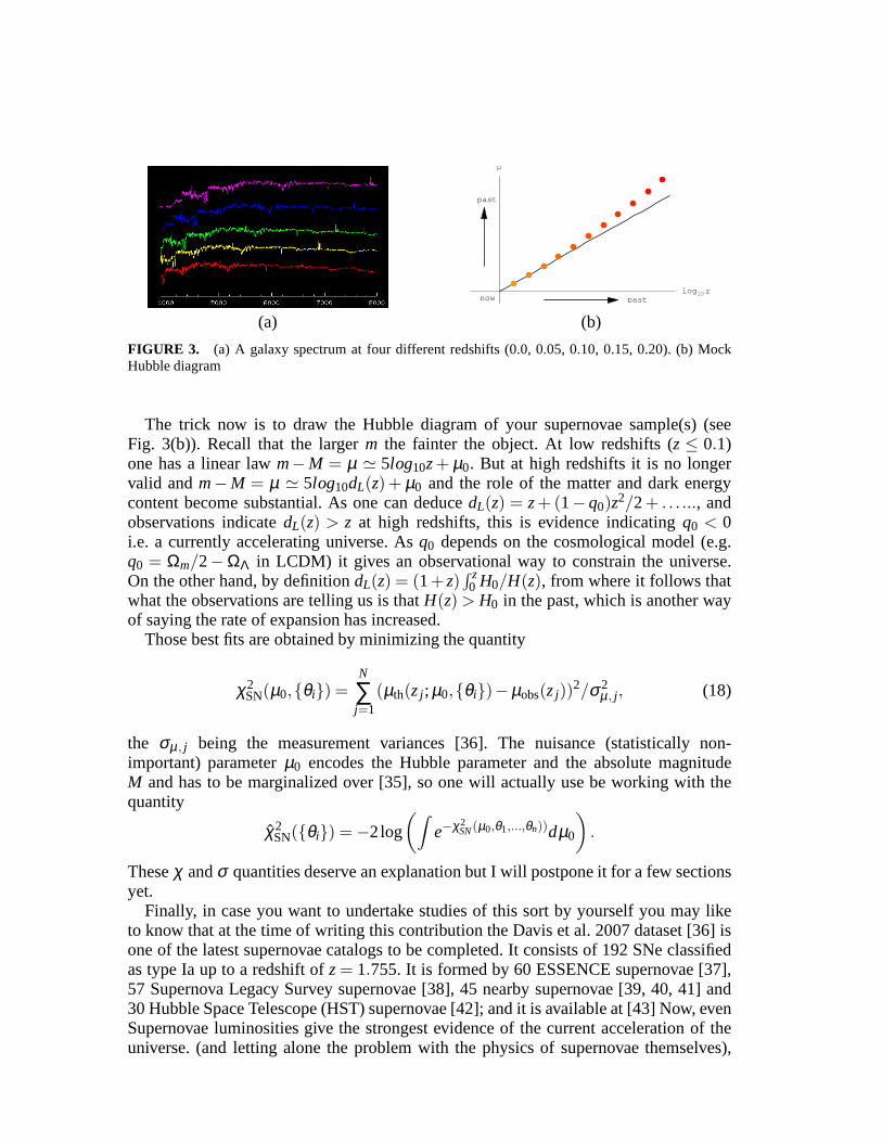
In what recession velocities are concerned it must be kept inmind that astronomicalobjects have characteristic spectral features due to the emission of specific wavelengthsof light from atoms or molecules. Templates exist which can be used to determine whichkind of object one is observing one basically compares different spectra till a best matchis found and which is the object’s redshift. Supernovae are assigned the redshift of theirhost galaxy; Fig. 3 (a) is a courtesy of SDSS1.

1Image courtesy of SDSS. Funding for the SDSS and SDSS-II has been provided by the Alfred P. Sloan Foundation, the Participating Institutions, the National Science Foundation, the U.S. Department

of Energy, the National Aeronautics and Space Administration, the Japanese Monbukagakusho, the Max Planck Society, and the Higher Education Funding Council for England. The SDSSWeb Site ishttp://www.sdss.org/. The SDSS is managed by the Astrophysical Research Consortium for the Participating Institutions. The Participating Institutions are the American Museumof Natural History, AstrophysicalInstitute Potsdam, University of Basel, University of Cambridge, Case Western Reserve University, University of Chicago, Drexel University, Fermilab, the Institute for Advanced Study, the Japan ParticipationGroup, Johns Hopkins University, the Joint Institute for Nuclear Astrophysics, the Kavli Institute for Particle Astrophysics and Cosmology, the Korean Scientist Group, the Chinese Academy of Sciences(LAMOST), Los Alamos National Laboratory, the Max-Planck-Institute for Astronomy (MPIA), the Max-Planck-Institutefor Astrophysics (MPA), New Mexico State University, Ohio State University, Universityof Pittsburgh, University of Portsmouth, Princeton University, the United States Naval Observatory, and the University of Washington.

log 10 z

Μ

now

past

past

(a) (b)

FIGURE 3. (a) A galaxy spectrum at four different redshifts (0.0, 0.05, 0.10, 0.15, 0.20). (b) MockHubble diagram

The trick now is to draw the Hubble diagram of your supernovaesample(s) (seeFig. 3(b)). Recall that the largerm the fainter the object. At low redshifts (z≤ 0.1)one has a linear lawm−M = µ ≃ 5log10z+ µ0. But at high redshifts it is no longervalid andm−M = µ ≃ 5log10dL(z)+ µ0 and the role of the matter and dark energycontent become substantial. As one can deducedL(z) = z+ (1−q0)z2/2+ . . . ..., andobservations indicatedL(z) > z at high redshifts, this is evidence indicatingq0 < 0i.e. a currently accelerating universe. Asq0 depends on the cosmological model (e.g.q0 = Ωm/2−ΩΛ in LCDM) it gives an observational way to constrain the universe.On the other hand, by definitiondL(z) = (1+z)

∫ z0 H0/H(z), from where it follows that

what the observations are telling us is thatH(z)> H0 in the past, which is another wayof saying the rate of expansion has increased.

Those best fits are obtained by minimizing the quantity

χ2SN(µ0,θi) =

N

∑j=1

(µth(zj ; µ0,θi)−µobs(zj))2/σ2

µ, j , (18)

the σµ, j being the measurement variances [36]. The nuisance (statistically non-important) parameterµ0 encodes the Hubble parameter and the absolute magnitudeM and has to be marginalized over [35], so one will actually usebe working with thequantity

χ2SN(θi) =−2log

(

∫

e−χ2SN(µ0,θ1,...,θn))dµ0

)

.

Theseχ andσ quantities deserve an explanation but I will postpone it fora few sectionsyet.

Finally, in case you want to undertake studies of this sort byyourself you may liketo know that at the time of writing this contribution the Davis et al. 2007 dataset [36] isone of the latest supernovae catalogs to be completed. It consists of 192 SNe classifiedas type Ia up to a redshift ofz= 1.755. It is formed by 60 ESSENCE supernovae [37],57 Supernova Legacy Survey supernovae [38], 45 nearby supernovae [39, 40, 41] and30 Hubble Space Telescope (HST) supernovae [42]; and it is available at [43] Now, evenSupernovae luminosities give the strongest evidence of thecurrent acceleration of theuniverse. (and letting alone the problem with the physics ofsupernovae themselves),

FIGURE 4. 68% and 95% confidence regions ofΩm andΩΛ from various current measurements, andexpected confidence region from the SNAP supernova program.Image courtesy of SNAP.

there is the problem of a certain degeneracy in the test (see Fig. 4) so supernovae donot provide a good individual estimate of the cosmological parameters. We will addresssome of those tests in the next sections.

HUBBLE PARAMETER FROM STELLAR AGES

There is a feverish activity in constraining parameters of the Universe. We are focusingin these lectures in the tests based solely on geometry. The first goal of these researchesis determining the current value of the equation of state parameterw. The next goal is todetermine its evolution, i.e. to draw its redshift history.The supernovae luminosity testis somewhat compromised by its integral nature:dL(z) = H0(1+ z)

∫ z0(1+ z′)(dt/dz′).

As an alternative, measures of the integrand of the latter have been proposed in [44] as away to improve sensitivity tow(z). That test relies on the availability of a cosmic clockto measure how the age of the Universe varies with redshift. Such a clock is provided byspectroscopy dating of galaxy ages. The idea is to obtain theage difference∆t betweentwo-passively evolving galaxies born approximately at thesame time but with a smallredshift separation∆z. One will then use∆t/∆z to inferdt/dz, as it is directly related tothe Hubble parameterH(z)=−(1+z)−1dz/dt, which is just the inverse of the integrandin the luminosity distance formula.

However, in Astrophysics important open questions about galaxy formation and evo-lution remain. How did a homogeneous universe become a clumpy one? Inflation drivesa major early homogeneization of the Universe but it also provides the primordial fluc-tuations which give rise to structure. How were galaxies born? How do they change over

time? Progress in understanding these questions will help making the most out of thistest.

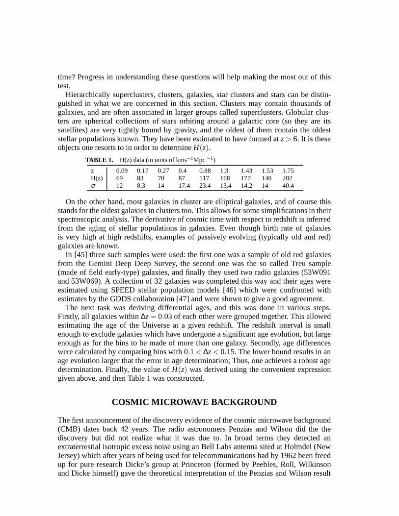
Hierarchically superclusters, clusters, galaxies, star clusters and stars can be distin-guished in what we are concerned in this section. Clusters may contain thousands ofgalaxies, and are often associated in larger groups called superclusters. Globular clus-ters are spherical collections of stars orbiting around a galactic core (so they are itssatellites) are very tightly bound by gravity, and the oldest of them contain the oldeststellar populations known. They have been estimated to haveformed atz> 6. It is theseobjects one resorts to in order to determineH(z).

TABLE 1. H(z) data (in units of kms−1Mpc −1)

z 0.09 0.17 0.27 0.4 0.88 1.3 1.43 1.53 1.75H(z) 69 83 70 87 117 168 177 140 202σ 12 8.3 14 17.4 23.4 13.4 14.2 14 40.4

On the other hand, most galaxies in cluster are elliptical galaxies, and of course thisstands for the oldest galaxies in clusters too. This allows for some simplifications in theirspectroscopic analysis. The derivative of cosmic time withrespect to redshift is inferredfrom the aging of stellar populations in galaxies. Even though birth rate of galaxiesis very high at high redshifts, examples of passively evolving (typically old and red)galaxies are known.

In [45] three such samples were used: the first one was a sampleof old red galaxiesfrom the Gemini Deep Deep Survey, the second one was the so called Treu sample(made of field early-type) galaxies, and finally they used tworadio galaxies (53W091and 53W069). A collection of 32 galaxies was completed this way and their ages wereestimated using SPEED stellar population models [46] whichwere confronted withestimates by the GDDS collaboration [47] and were shown to give a good agreement.

The next task was deriving differential ages, and this was done in various steps.Firstly, all galaxies within∆z= 0.03 of each other were grouped together. This allowedestimating the age of the Universe at a given redshift. The redshift interval is smallenough to exclude galaxies which have undergone a significant age evolution, but largeenough as for the bins to be made of more than one galaxy. Secondly, age differenceswere calculated by comparing bins with 0.1< ∆z< 0.15. The lower bound results in anage evolution larger that the error in age determination; Thus, one achieves a robust agedetermination. Finally, the value ofH(z) was derived using the convenient expressiongiven above, and then Table 1 was constructed.

COSMIC MICROWAVE BACKGROUND

The first announcement of the discovery evidence of the cosmic microwave background(CMB) dates back 42 years. The radio astronomers Penzias andWilson did the thediscovery but did not realize what it was due to. In broad terms they detected anextraterrestial isotropic excess noise using an Bell Labs antenna sited at Holmdel (NewJersey) which after years of being used for telecommunications had by 1962 been freedup for pure research Dicke’s group at Princeton (formed by Peebles, Roll, Wilkinsonand Dicke himself) gave the theoretical interpretation of the Penzias and Wilson result

as a prediction of the big bang models. Two papers [4, 5] were sent jointly and appearedin the 142th volume of the Astrophysical Journal, the Penzias and Wilson paper washumbler, but they got rewarded years later (in 1978) with theNoble Prize. Theoreticaladvances and predictions on the topic had been done earlier by Gamow, Alpher andHerman, and although the Princeton group had drawn their conclusions independently,one of his members, Peebles, recognized the contribution ofthose authors in his classicaltextbook [48]. Just a few months after the publication of thementioned two papers,Roll and Wilkinson [6] confirmed in another work the thermal nature of the spectrumof the radiation (in concordance with the big bang model prediction) and estimated itstemperature to be about 3.0±0.5K.

The next major breakthrough in this topic was the discovery of the CMB anisotropiesby the COBE satellite, and as a consequence Cosmology got twomore Nobel laureates in2006: Smooth and Mather. According to the calculations carried out by Harrison [49],Peebles and Yu [50], and independently by Zeldovich [51], CMB anisotropies are theconsequence of the predictable primeval inhomegeneities of amplitude 10−5.

The CMB power spectrum, through its pattern of peaks (see Fig. 5(a)), tell us that theUniverse is very close to spatially flat (at a high degree of accuracy) (see for instance[52] among the also vast amount of references mentioning this). The CMB also informus that inflation was the major component of cosmic structureformation as opposed tocosmic strings (for a short history of the discovery of the first peak see [53])

You may already be convinced that CMB physics is capital. On the one hand no othercosmological probe has beaten it so far in the amount of relevant information it provides,and on the other hand it supports the big bang model and links Cosmology and particlephysics as the observed abundances of light elements determined from measurementsof the fluctuations of the cosmic background radiation temperature are in agreementwith big bang nucleosynthesis [54], being based on the well-trusted Standard Model ofParticle physics. But the list of important pieces of information it gives us does not endthere as it provides traces of very weak primordial fluctuations which may have seededthe large scale structure observed today, it informs us of the geometry of the universe(first peak), it provides evidence for baryonic dark matter (second peak), it constrainsthe amount of dark matter (third peak) [55] and finally, a factwhich is very important tous is that constraints on dark energy models can be refined using CMB data.

At this stage is it convenient to make a thermal history sketch (as illustrated in Fig.5(b)). After the big bang the Universe cools down due to adiabatic expansion and its goesthrough these stages: the energies of particles decrease and several phase transitionsoccur, massive particles become non-relativistic as temperature decreases below theirrest mass, the rates of production of particle-antiparticle decrease and anhilitation leavesasymmetric populations, nuclei of light elements form (z ≃ 104) and the Universebecomes a soup of nucleons, photons and free electrons (the CMB forms atz≃ 107).

As the density of relativistic particles decreases faster (proportional toa−4) than thatof non-relativistic ones (proportional toa−3) at some stage one gets matter-radiationequality. Later on, thermal ionization ceases to be effective, atoms form (z ≃ 104)electrons get bound to nucleons (recombination) and photons decouple and travel freelyto us since [56, 57]

Just to give a few more details about the formation of the CMB background let usmention that it formed during the epoch 1010> z> 107 due to photon creation processes

(a) (b)

FIGURE 5. (a) WMAP angular temperature power-spectrum. (b) Timelineof the universe. Imagekindly produced by Raúl B. Pérez-Sáez.

(bremsstrahlung and double Compton scattering) [58]. At later stages the dominantcoupling effect turned to be Compton/Thompson scattering but it did not destroy thethermal nature of the spectrum.

The basic observable in CMB physics is temperature fluctuation ∆T/T (a field de-pending on direction on the sky). Initial density fluctuations were tiny, with an ampli-tude of about 10−5 so their evolution is linear, i.e. Fourier modes evolve independently.These primordial irregularities give rise to potential wells and hills according to whichthe baryons and the photons get accommodated. Photons, climb up (down) potentialwells (hills) in an unimpeded trip to us after getting released at the decoupling redshiftzdec≈ 1100 and give us a snap-shot of the early universe in the form of cold and redspots. This is a primary anisotropy that gets imprinted on the CMB at last scatteringresponsible for the characteristic large scale anisotropycalled Sachs-Wolfe plateau [59](this anisotropy is associated with fluctuations with period so large they have had notime to perform a complete oscillation by the recombinationtime [60]).

Let us now discuss were the peaks and troughs come from. Photon pressure suppliesforce: ∇pγ = ∇ργ/3, ργ ∼ T4, and the spatial variations of density themselves arealso a source of changes in the gravitational potential. Potential and pressure gradientscompete between them and induce acoustic oscillations in the fluid which result intemperature oscillations∆T ∼ δρ1/4

γ ∼ A(k)cos(kcst), (harmonic wave), with cs thespeed of sound. This photons do not find opposition either between their departure andtheir arrival to their destination (our observing devices). Photons released at maximumcompression give blue spots as they have to climb up the potential, so they appear blueto us. In contrast, those caught at maximum rarefaction formred spots. In summary, thepattern of spots associated with long wavelength perturbations gets enriched by thosecoming from perturbations with smaller wavelengths.

That of course, is not the end of the explanation, the angularpower spectrum is thefunction describing how the variance of the fluctuations depends on the angular scale (itsdefinition rests on the assumption of Gaussianity and randomness of the fluctuations).Fluctuation extrema correspond to peaks in power (even onescorrespond to compressionand odd ones correspond to rarefaction). Randomness of the fluctuations implies wehave them in all wavelenghts, and clearly and when we comparea fluctuation of a given

wavelength with another one with half of that wavelength it is obvious that the time thesecond takes to complete an oscillation is half of the time the first one takes. Thus, if byrecombination there is a mode which has completed half an oscillation, there will modeswhich will have completed 2,3,4, . . . half oscillations.

You may have noticed, as well, that the spectrum presents a modulation, it is due todifferent effects (see [61] for an authorized discussion).Baryons being massive havepreference for the throughs and the compression gets enhanced, thus the amplitude ofodds peaks gets larger. Another effect of baryons is making the oscillations slower sothe peaks are pushed to higher multipoles. On the other hand,photons are also importantin the modulation as in the radiation dominated phase. During radiation dominationmost gravity comes from photons, they are the major source ofgravitational potentialso as pressure redistributes the photons, gravitational potentials get washed away. Thiseffect is absent when the Universe becomes matter dominated, so it is exclusive to highfrequency modes, whereas low frequency modes do not start tooscillate till matterdomination has begun. Finally, there is also a strong damping effect due to slightimperfections in the fluid associated with shear viscosity and heat conduction (Silkdamping [62]).

Interestingly, the CMB provides a dark energy test which requires considering onlythe background geometry, in contrast to other uses which rest on the powerful but chal-lenging study of perturbations. This is the CMB shift test, which estimates how a physi-cal length in the primordial universe appears to us. By comparing the (non-Euclidianity)effects on geometry of different matter/contents inference about the likeliest ones can bedone. The basic quantity to consider is that in an arbitrary model the position of the firstpeak in the temperature spectrum isl1 = πDA(zrec)/rs(zrec), where the quantityrs(zrec)represents the last scattering sound horizon scale i.e. thedistance sound may travel be-fore the recombination epoch.

The CMB shift gives the first CMB peak position ratio between amodel one wants totest (unprimed model) and a reference Einstein-de Sitter model (primed model)

R≡ 2l1/l′1

[63] It is considered as a robust test as it does not depend on the parameterH0 (theHubble factor today), which is not constrained by the other tests. Considering the speedof soundcs is constant and using the approximations

D′A(zrec)≈ 2carec/H0 rs(zrec)≈ 2csa

3/2rec/H0

√

Ωm, (19)

one finally arrives at

R≈ H0

√

Ωm

∫ zrec

0dz/H(z). (20)

You can go by the valueR(1089) = 1.71±0.03 calculated from WMAP3 data.In a fashion similar to the other tests one will have to construct aχ2 function using

the latter observational value and the theoretical function for the cosmological model tobe constrained.

In the next section we are going to consider a test which also stems from early universephysics.

FIGURE 6. Two stages in the evolution of a primordial density perturbation. Baryon density is on theleft panels, photon density middle ones and mass profile in the right panel. The upper image is for asituation not much later than the decoupling time, the last one correspond to much later epoch. Imagescourtesy of Martin White.

BARYON ACOUSTIC OSCILLATIONS

Diagnosing the mystifying new physics causing acceleration requires more precise mea-surements of cosmological distance scales. In recent yearsa new geometrical constraintof dark energy has emerged which relies on traces left by early universe sound waves inthe galaxy distribution. This test is somehow in its infancybut it is very promising. Asit often in science, quite a few years have elapsed form prediction of the effect [64, 65]till its detection [66].

Let me move on now to a physical description of the phenomenonbased on the onefound in [67] (see as well [68, 69]). The early universe was composed of a plasma ofenergetic photons and ionized hydrogen (protons and electron) in addition to other traceelements. Imagine now a single perturbation in the form of a excess of matter. Pressure isvery high and ejects the baryon-photon outward at relativistic velocities. At first photonand baryons go by the hand (the speed of the radius of the shellbeing larger than half thespeed of light). At recombination photons decouple and stream away whereas the baryonpeak gets frozen; the reason for this is they are cold dark matter and therefore they haveno intrinsic motion (no pressure) unlike the previous stages where they were coupledto the photons (in this early situation baryons were subjectto radiation pressure). Thephoton distributions become more and more homogeneous, while the baryon overdensitydoes not disappear. Finally, the initial large gravitational potential well begins to attractmatter back into it and a second overdense region appears at the center. Two stages inthe evolution of a single perturbation are illustrated in Fig. 6

The most important fact of the phenomenon is it leaves traceable effects on large-scalestructure. Initial perturbations would have produced wavyexcitations emanating from allpoints, and the subsequent evolution would resemble what happens when dropping rocksin a pond. The plasma shells would have today 150 Mpc (or 500 million light years)and galaxy formation in the locus of those shells would be likelier. In fact, there is a

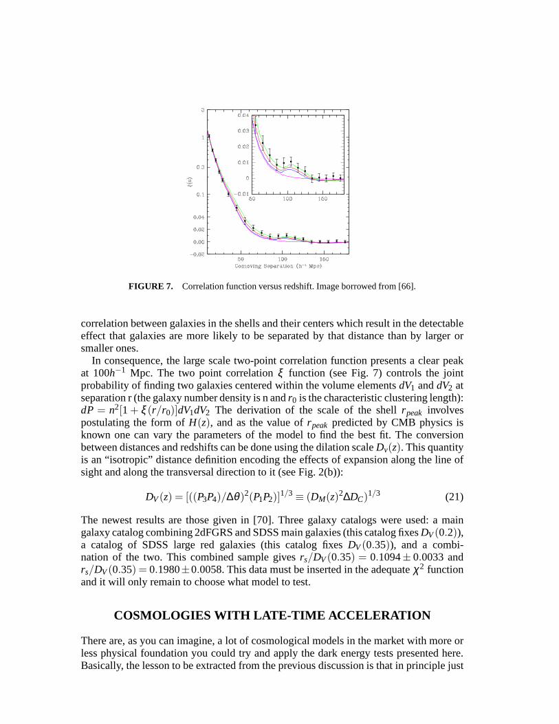
FIGURE 7. Correlation function versus redshift. Image borrowed from[66].

correlation between galaxies in the shells and their centers which result in the detectableeffect that galaxies are more likely to be separated by that distance than by larger orsmaller ones.

In consequence, the large scale two-point correlation function presents a clear peakat 100h−1 Mpc. The two point correlationξ function (see Fig. 7) controls the jointprobability of finding two galaxies centered within the volume elementsdV1 anddV2 atseparation r (the galaxy number density is n andr0 is the characteristic clustering length):dP = n2[1+ ξ (r/r0)]dV1dV2 The derivation of the scale of the shellrpeak involvespostulating the form ofH(z), and as the value ofrpeak predicted by CMB physics isknown one can vary the parameters of the model to find the best fit. The conversionbetween distances and redshifts can be done using the dilation scaleDv(z). This quantityis an “isotropic” distance definition encoding the effects of expansion along the line ofsight and along the transversal direction to it (see Fig. 2(b)):

DV(z) = [((P3P4)/∆θ)2(P1P2)]1/3 ≡ (DM(z)2∆DC)

1/3 (21)

The newest results are those given in [70]. Three galaxy catalogs were used: a maingalaxy catalog combining 2dFGRS and SDSS main galaxies (this catalog fixesDV(0.2)),a catalog of SDSS large red galaxies (this catalog fixesDV(0.35)), and a combi-nation of the two. This combined sample givesrs/DV(0.35) = 0.1094± 0.0033 andrs/DV(0.35) = 0.1980±0.0058. This data must be inserted in the adequateχ2 functionand it will only remain to choose what model to test.

COSMOLOGIES WITH LATE-TIME ACCELERATION

There are, as you can imagine, a lot of cosmological models inthe market with more orless physical foundation you could try and apply the dark energy tests presented here.Basically, the lesson to be extracted from the previous discussion is that in principle just

needs to postulate the functional form ofH(z). In what follows I wish to make an aoutline of a few ot these models. This is, of course, a biased list of parameterizations asit is based on my own preferences, and on the other hand there are authorized reviewsyou can head to for a more exhaustive revision.

In general, a given general relativistic model of dark energy with equation of statewde(z) leads to

H2(z)/H20 = Ωm(1+z)3+(1−Ωm)exp

[

3∫ z

0(1+wde(x))/(1+x)dx

]

. (22)

To get the latter a universe containing dark energy and dust (dark matter and baryons)has been assumed.

The first model I want to consider here is theLCDM model. It follows from thechoicewde(z) =−1, i.e. dark energy is a cosmological constant. Thus

H2(z)/H20 = Ωm(1+z)3+1−Ωm, (23)

with Ωm a free parameter. LCDM is consistent with all data, but thereis a theoreticalproblem in explaining the observed value of the cosmological constantΛ.

The second case of this list is theDGP model It was proposed by Deffayet [71]the inspiration being [72] It represents a simple alternative to the standard LCDMCosmology, with the same number of parameters. Late-time acceleration in this modelis due to an infrared modification of gravity (no dark energy needed). Explicitly one has

H(z)/H0 = (1−Ωm)/2+√

(1−Ωm)2/4+Ωm(1+z)3. (24)

Let me now tell you about theQCDM model. It is the simplest generalization of theLCDM model. It consists in taking a constant value ofwde= w different in general from−1, so

H2(z)/H20 = Ωm(1+z)3+(1−Ωm)(1+z)3(1+w). (25)

Even though it is a rather simple model, it can be useful for detecting at a first instancepreference for evolutionary dark energy.

Another two parameter model of interest is theLDGP model [73]. The DGP modelhas actually two separate branches They reflect the two ways to embed the 4D braneuniverse in the 5D bulk spacetime. We have loosely called before DGP before to the self-accelerating branch (this is common practice in the literature) but I insist there is anotherbranch which is physically interesting too. The LDGP model precisely represents thisbranch, i.e. the non self-accelerating one, with a cosmological constant included whichis required for acceleration. Interestingly, higher values of the cosmological constant areallowed as compared to LCDM (due to an screening effect). In aexplicit way

H(z)/H0 =

√

Ωm(1+z)3+1−Ωm+2√

Ωrc +Ωrc −√

Ωrc (26)

and the parameterΩrc encodes the so called crossover scale signaling the transition fromthe general relativistic to the modified gravity regime

The last but one case I wish to address isChevallier-Polarski-Linder Ansatz [74].This is a widespread generalization of QCDM for which

wde(z) = w0+w1(1−1/(1+z)).

Therefore

H2(z)/H20 = Ωm(1+z)3+(1−Ωm)(1+z)3(1+w0+w1)e−3w1z/1+z. (27)

Two nice properties of it stand out, firstly the model displays finiteness ofH(z) at highredshifts, secondly it admits a simple physical interpretation asw1 is a measure of thescalar field potential slow roll factorV ′/V in a quintessence picture [76]

Finally, to put and end on this list, I would like to consider the QDGP model[75]. This is a generalization of LDGP: the cosmological constant is replaced by darkenergy with a constant equation of statew. The modified 4D Friedman equation has thefollowing form:

H(z)/H0 =

√

Ωm(1+z)3+(1−Ωm+2√

Ωrc)(1+z)3(1+w)+Ωrc −√

Ωrc.(28)

A remark about three of the models considered is in order. Models with late-timeacceleration due to infrared modifications of gravity are called dark gravity models, andDGP, LDGP and QDGP are of that sort. An effective dark energy equation of stateweffcan be deduced by imposingρeff + 3H(1+weff)ρeff = 0. Calculating this in terms ofredshift for the three models considered here can be a nice exercise for the readers.

I finish here this section as a turn of subject is required, as Ifeel this contributionwould not be sort of self-contained if the issue of the statistical treatment of the testsconsidered was not covered.

STATISTICAL INFERERENCE

Science, and ergo Astronomy, is about making decisions. Allscientific activities (de-sign of experiments, design and building of instruments, data collection, reduction andinterpretation, ...) rely on decisions. In turn, decisionsare made by comparison, andcomparison requires a statistics (a summarized description) of the available data. Theterm “statistics” means rigorously a quantity giving broadrepresentation of the data, butthe same term is also loosely used when referring to “statistical inference”. Moreover,as in science making decisions involves measurements and derivation of values of pa-rameters, it is necessary to assess the degree of belief of the true value of the parameterbeing measured/derived.

Astronomy/Cosmology being about the study of the Universe makes them singular inwhat concerns decision making. The Universe is not an experiment one can rerun, and tomake things worse the typical objects studied are very distant. In consequence, typicallyone will have very poor knowledge of the distribution behindthe variables subject tomeasurement. Yet the difficulties must be overcome as statistics enters all five stages inthe loop characterizing every experiment: observe-reduce-analyse-infer-cogitate.

I am going to introduce now some basic notions, definitions and notation to be usedhere after. "The readers interested in learning more about most of the topics addressedin this section can head to [77], but I also recommend to you other sources such as[78, 79, 81].

Probability will be a numerical account of our strength of belief. Let us enunciate nowKolmogorov axioms: for any random eventA one has 0< prob(A)< 1, if and eventA iscertain thenprob(A) = 1, if eventA andB are exclusive, thenprob(AorB) = prob(A)+prob(B). These axioms are basically all is needed to develop entirely the mathematicalprobability theory (by this one means the recipes to manipulate probabilities once theyhave been specified). Probabilities are not inherent properties of physical problems, thatmeans they do not make sense on their own, they are just a reflection of the knowledgewe have.

If the knowledge about evenA does not affect the probability of eventB, thoseevents are independent, i.e.prob(Aand B) = prob(A)prob(B). If A and B arenot independent events then it is convenient to know conditional probabilities:prob(A|B) = prob(Aand B)/prob(B) and prob(B|A) = prob(Aand B)/prob(A),which can be derived from Kolmogorov axioms. IfA and B are independent, thenprob(A|B) = prob(A) prob(B|A) = prob(B) In addition, if eventB comes is dif-ferent flavours(B1,B2,B3, ...), then p(A) = ∑i prob(A|Bi)prob(Bi). Moreover, if Ais a parameter of insterest but theBi are not, knowledge ofprob(Bi) allows gettingrid of those nuisance parameters by summation/integration, and the process is calledmarginalization.

Having presented this basics let me guide you into the realm of Bayesian infer-ence By equatingprob(Aand B) and prob(Band A) one gets the identityprob(A|B) =prob(B|A)prob(B)/prob(A) known as Bayes theorem.

There is a state of belief, the priorprob(B), before the data, the eventA, are col-lected, and experience modifies this knowledge. Experienceis encoded in the likelihood,prob(A|B). The state of belief at the end of the process (analysis of thedata) is repre-sented by the posteriorprob(B|A). Mathematically naïve though it is, this theorem is, aregards interpretation, very powerful, but not devoid of controversy. I provide here onlya short account of Bayesian statistics, if you feel like learning more about it, head to thissite [80].

For a better understanding of the different between the Bayesian and frequentistapproaches, consider now taking out balls from a box (you cannot see the inside andonly know they are either white or red). Imagine you extract several times three balls andput them back into the box. Would you care of the probability of taking out two whitesand one red? Would you rather not be more interested in sayingsomething about thecontents of the box? The second question seems the more natural one. This is the kind ofquestion Bayes theorem allows to answer. Bayesians care forprobabilities of hypothesesgiven data, whereas frequentists are concerned about the probability of hypothetical dataassuming the truth of some hypothesis.

A useful concept in connection with all this is that of probability density functions.If x is a random real variable expressing a result, the probability of getting a numbernear x isp(x) = prob(x)δx, and p(x) is the probability density function distributionof x (probability density functions are also called probability distributions). Probability

density functions satisfy these properties:prob(a< x< b) =∫ b

a p(x)dx,∫ ∞−∞ p(x)dx= 1,

p(x) is single-valued and non-negative for all realx. Probability density functions areusually quantified by the position of the center or meanµ =

∫ ∞−∞ xp(x)dx, the spread

σ2 =∫ ∞−∞(x−µ)2p(x)dx.

Among them one stands out notoriously; it is the Gaussian probability density func-tion, which is an ubiquitous distribution in Physics, thanks to the central limit theorem,which makes it work is most situations: broadly speaking a little averaging makes anydistribution converge to the Gaussian one, explicitly,p(x) = e−(x−µ)2/σ/

√2πσ .

We are going to make use of it for parameter estimation and model selection, whichis at the core of many investigations in Cosmology these days. Consider we haveNobservational data for some physical quantityf th of interest. We set f obs

j = d j.

Assumef th depends on parametersθi and consider it in the context of a given modelM . In addition, regard the errors as Gaussian distributed so the likelihood reads

L (d j|θi,M ) ∝ e−χ2(θi) with χ2(θi) =N

∑j=1

[ f obsj − f th(θi)]2/σ2

j . (29)

For uncorrelated observational datasets

L (d(1)j ∩ . . .∩d(m)

k |θiM ) ∝ L (d(1)j |θiM )× . . .×L (d(m)

k |θiM ).(30)

The probability density functionp(θi|d j,M ) of the parameters to have valuesθi under the assumption that the true model isM and provided that the availableobservational data ared j is given by Bayes theorem. In terms of probability densityfunctions

p(θi|d j,M ) =L (d j|θi,M )π(θi,M )

∫

L (d j|θi,M )π(θi,M )dθ1 . . .dθn. (31)

Here p(θi|d j,M ) is called the posterior probability density function. and best fitvalues of the parameters are estimated by maximizing it, whereasπ(θi,M ) is calledthe prior probability density function. Choice of prior is subjective but compulsory inthe Bayesian approach; remember the prior pdf encodes all previous knowledge aboutthe parameters before the observational data have been collected.

The first step to estimate parameters in the Bayesian framework is maximizing theposterior p(θi|d j, |M ). The second step is construction credible intervals It isconvenient to simplify our notation, sop(θi|d j,M )≡ p(θ1, . . . ,θn). The marginalprobability density function onθi is p(θi) =

∫

p(θ1, . . . ,θn)dθ1 . . .dθi−1dθi+1 . . .dθn.Of course, if the model is genuinely uniparametric no marginalization is required. It isalso convenient to define parametersθil andθiu satisfyingp(θil )≃ 0 andp(θiu)≃ 0 Thecredible intervals, under the hypothesis that the marginalpdf is approximately Gaussian,are constructed from the median and errors. The 68% percent credible intervals on theparameterθi are given asθi = x+z

−yThe medianx is calculated from

∫ xθil

p(θi)dθi = 0.5×∫

p(θi)dθi The lower errory

is calculated from∫ x−y

θilp(θi)dθi = ((1−0.68)/2)×

∫

p(θi)dθi The upper errorz is

calculated from∫ θiu

x+z p(θi)dθi = ((1−0.68)/2)×∫

p(θi)dθi

Credible contours are a popular/illustrating construction and they are worth a mention.By marginalization with respect to all parameters but two one gets

p(θi ,θi+1) = p(θi) =∫

p(θ1, . . . ,θn)dθ1 . . .dθi−1dθi+2 . . .dθn

Again, obviously, marginalization is not necessary if the model is genuinely biparamet-ric. An effectiveχ2 can be defined in the form−2log(p(θi,θi+1)) = χ2

e f f(θi ,θi+1)/2(up to a constant), so the best fit responds to the maximum posterior criterion. The prob-ability that for some parameters other than those for the best fit (maximum likelihood)χ2 increases with respect to the best fit by an amount∆χ2 is 1−Γ(1, log(pb f/p))/Γ(1).By fixing the desired probability content, the latter becomes the implicit equation of thecredible contours on the parameter space (popular choices in the literature are 68.3%,95.4% and 99.7%).

Now let me comment about model selection. Bayesians use a estimator to selectmodels which informs about how well the parameters of the model fit the data. It doesnot rely exclusively on the best-fitting parameters of the model, but rather it involvesan averaging over all the parameter values that were theoretically plausible before themeasurement ever took place [81]. Bayes evidence is

E (M ) = p(d j|M ) =

∫

π(θi,M )L (d j|θi,M )dθ1 . . .dθn, (32)

so it is the probability of datad j given the modelM Hereπ(θi,M ) is the model’sprior on the set of parameters, normalized to unity (i.e.

∫

π(θi,M )dθ1 . . .dθn= 1.)Using the popular top-hat priorπ(θi) = (θimax−θimin)

−1 Bayes evidence is rewritten as

E (M ) =

(

∫ θ1max

θ1min

. . .

∫ θnmax

θnmin

L (θ1, . . . ,θn)dθ1 . . .θn

)

/

(

∫ θ1max

θ1min

. . .

∫ θnmax

θnmin

dθ1 . . .dθn

)

.

Finally, preference of modelMi over modelM j givendk is estimated by

p(Mi |dk)/p(M j |dk) = Ei(Mi)πi(Mi)/E j(M j)π j(M j)

The Bayes factorBi j for any two modelsMi andM j is

Bi j = Ei(Mi)/E j(M j)

so if as in usual practice one assumes no prior preference of one model over the other,that is, Assumingπi(Mi) = π j(M j) = 1/2 (noa priori preference) then

p(Mi|dk)/p(M j |dk) = Bi j .

The most popular key to interpreting Bayes factors is Jeffreys scale [82]: ifln(Bi j )< 1,then the evidence againstM j is not significant, if 1< ln(Bi j ) < 2.5, then the evidenceagainstM j is substantial, if 2.5< ln(Bi j )< 5, then the evidence in favor ofMi is strong,if 5 < ln(Bi j ), then the evidence in favor ofMi is decisive.

There are of course many more things which could be mentionedabout this topic, butI hope this condensed introduction will help you start crossing swords with the art ofconstraining dark energy models using geometrical tests like the ones discussed here orupcoming ones.

CONCLUSIONS

In this contribution I have tried to review some of the background on geometrical testsof dark energy models. A historical review of the development of Cosmology has beenfollowed by an account of the importance of the discovery of the late-time acceleration,which is commonly attributed to the existence of an exotic component in the cosmicbudget. Other possible explanations have been attempted, which required being openminded enough to admit the existence of extra dimensions.

Examples of both conventional (if that adjective can be used) and extradimensionalmodels have been mentioned here with respect to their geometrical features. All thesemodels can be subject to different observational tests which only require postulatinga parametrization of the Hubble factor of the Universe or quantities derived from it.Here I have been concerned with four tests only: luminosity of supernovae, directH(z) measurements, the CMB shift and baryon acoustic oscillations. I cannot deny thisselection is biased in the sense these are tests I have made research on, but the first andthe last one are definitely very important and much effort is doing by research groups allover the world in finding the data their application requires.

This contribution has also tried to maintain a pedagogical tone as it has been preparedfor the Advanced Summer School 2007 organized by Cinvestav in Mexico DF. I justhope it will be useful to any reader which happens to come across it.

ACKNOWLEDGMENTS

I wish to thank to Nora Bretón, Mauricio Carbajal and Oscar Rosas-Ortiz for giving methe opportunity to present this contribution to the Advanced School Summer School inPhysics 2007 at Cinvestav. I am also much indebted to Elisabetta Majerotto, as I haveborrowed part of the material presented in this lectures I have borrowed from work donein collaboration with her. Finally, I wish to thank Mariam Bouhmadi and again NoraBretón for reading the manuscript and helping improving it and to Raúl B. Pérez-Sáezfor a lovely picture.

REFERENCES

1. Henry E. Kandrup, “Conversational Cosmology”, unpublished.2. http://en.wikipedia.org/wiki/Physical_Cosmology3. M. S. Turner, Phys. Today,56 (2003) 104. A. A. Penzias and R.W. Wilson, Astrophys. J.142 (1965) 4195. R. H. Dicke, P. J. E. Peebles, P. G. Roll and D. T. Wilkinson,Astrophys. J.142 (1965) 4146. P. G. Roll and D. T. Wilkinson, Phys. Rev. Lett.16 (1966) 4057. http://background.uchicago.edu/8. A. G. Riesset al.[Supernova Search Team Collaboration], Astron. J.116 (1998) 1009 [arXiv:astro-

ph/9805201].9. S. Perlmutteret al. [Supernova Cosmology Project Collaboration], Astrophys.J. 517 (1999) 565

[arXiv:astro-ph/9812133]10. S. Perlmutter, Phys. Today,56 (2003) 5311. http://mapg.gsfc.nasa.gov/m_uni/uni_101matter.html12. M. Tegmark, arXiv:0709.4024 [physics.pop-ph]

13. J. Yadav, S. Bharadwaj, B. Pandey and T. R. Seshadri, Mon.Not. Roy. Astron. Soc.364 (2005) 601[arXiv:astro-ph/0504315]

14. T. Souradeep, A. Hajian and S. Basak, New Astron. Rev.50 (2006) 889 [arXiv:astro-ph/0607577]15. R. Trotta and R. Bower, Astron. Geophys.47 (2006) 4:20 [arXiv:astro-ph/0607066]16. R. D’Inverno, “Introducing Einstein’s Relativity”, Oxford University Press (1992)17. M. Trodden and S. M. Carroll, arXiv:astro-ph/040154718. L. Bergström and A. Goobar, “Cosmology and Particle Astrophysics”, Springer (2006)19. J.A. Peacock, “Physical Cosmology”, Cambridge University Press (1999)20. V. Sahni, arXiv:astro-ph/021108421. V. Gorini, A. Kamenshchik and U. Moschella, Phys. Rev. D67 (2003) 063509 [arXiv:astro-

ph/0209395]22. M. C. Bento, O. Bertolami and A. A. Sen, Phys. Rev. D66 (2002) 043507 [arXiv:gr-qc/0202064]23. S. Nojiri and S. D. Odintsov, Phys. Rev. D72, 023003 (2005) [arXiv:hep-th/0505215]24. I. Zlatev, L. M. Wang and P. J. Steinhardt, Phys. Rev. Lett. 82, 896 (1999) [arXiv:astro-ph/9807002]25. C. Armendariz-Picon, V. F. Mukhanov and P. J. Steinhardt, Phys. Rev. D63, 103510 (2001)

[arXiv:astro-ph/0006373].26. A. Sen, JHEP0204, 048 (2002) [arXiv:hep-th/0203211]27. Z. K. Guo, Y. S. Piao, X. M. Zhang and Y. Z. Zhang, Phys. Lett. B 608 (2005) 177 [arXiv:astro-

ph/0410654].28. D. W. Hogg, arXiv:astro-ph/990511629. A. V. Filippenko, Ann. Rev. Astron. Astrophys.35 (1997) 30930. D.H. Clark, F.R. Stephenson, “The Historical Supernovae”, Pergamon Press (1977)31. “HST Data Hand Book”,http://www.stsci.edu32. http://www.astro.wisc.edu/˜jsg/astro335/class_pdf_m aterials/

magnitudes_jan31_02.pdf33. S. Perlmutteret al. [Supernova Cosmology Project Collaboration], Astrophys.J. 483 (1997) 565

[arXiv:astro-ph/9608192]34. A. Kim, A. Goobar and S. Perlmutter, Publ. Astron. Soc. Pac. 108 (1996) 190 [arXiv:astro-

ph/9505024]35. S. L. Bridle, R. Crittenden, A. Melchiorri, M. P. Hobson,R. Kneissl and A. N. Lasenby, Mon. Not.

Roy. Astron. Soc.335 (2002) 1193 [arXiv:astro-ph/0112114]36. T. M. Daviset al., arXiv:astro-ph/070151037. W. M. Wood-Vaseyet al., arXiv:astro-ph/070104138. P. Astieret al., Astron. Astrophys.447 (2006) 31 [arXiv:astro-ph/0510447]39. M. Hamuy, M. M. Phillips, N. B. Suntzeff, R. A. Schommer and J. Maza, arXiv:astro-ph/960906440. A. G. Riesset al. [Supernova Search Team Collaboration], Astron. J.116 (1998) 100941. S. Jha, A. G. Riess and R. P. Kirshner, Astrophys. J.659 (2007) 122 [arXiv:astro-ph/0612666]42. A. G. Riesset al., arXiv:astro-ph/061157243. http://www.dark-Cosmology.dk/archive/SN .44. R. Jiménez and A. Loeb, Astrophys. J.573 (2002) 37 [arXiv:astro-ph/0106145]45. J. Simon, L. Verde and R. Jiménez, Phys. Rev. D71 (2005) 123001 [arXiv:astro-ph/0412269]46. R. Jiménez, J. MacDonald, J. S. Dunlop, P. Padoan and J. A.Peacock, Mon. Not. Roy. Astron. Soc.

349 (2004) 240 [arXiv:astro-ph/0402271]47. P. J. McCarthyet al., Astrophys. J.614 (2004) L9 [arXiv:astro-ph/0408367]48. P. J. E. Peebles, “Principles of Physical Cosmology", Princeton University Press (1993)49. E. R. Harrison, Phys. Rev. D1 (1970) 272650. P. J. E. Peebles and J. T. Yu,Astrophysical Journal 162 (1970) 81551. Ya. B. Zel’dovich, Mon. Not. Royal Astr. Soc. 160 (1972) 152. http://www.sarahbridle.net/lectures/uclgrad07/lss_a nd_cmb.pdf53. http://background.uchicago.edu/ whu/intermediate/fir stdata.html54. D. N. Schramm and M. S. Turner, Rev. Mod. Phys.70 (1998) 303 [arXiv:astro-ph/9706069]55. http://www.strw.leidenuniv.nl/education/courses/mo2 005/

pdf/CMB_fluctuations.pdf56. http://pdg.lbl.gov/1998/microwaverpp_part1.pdf57. W. Hu and J. Silk, Phys. Rev. D48 (1993) 48558. M. Birkel and S. Sarkar, Phys. Lett. B408 (1997) 59 [arXiv:hep-ph/9705331]

59. C. H. Lineweaver, arXiv:astro-ph/970204260. http://astro.berkeley.edu/˜mwhite/rosetta/node6.html61. W. Hu and S. Dodelson, Ann. Rev. Astron. Astrophys.40 (2002) 171 [arXiv:astro-ph/0110414].62. J. Silk, Astrophys. J. 151 (1968) 45963. J. R. Bond, G. Efstathiou and M. Tegmark, Mon. Not. Roy. Astron. Soc.291 (1997) L33

[arXiv:astro-ph/9702100]64. S. Bashinsky and E. Bertschinger, Phys. Rev. Lett.87 (2001) 081301 [arXiv:astro-ph/0012153]65. R. A. Sunyaev and Y. B. Zeldovich, Astrophys. Space Sci.7 (1970) 366. D. J. Eisensteinet al. [SDSS Collaboration], Astrophys. J.633 (2005) 560 [arXiv:astro-

ph/0501171]67. http://astro.berkeley.edu/˜mwhite/bao/68. D. J. Eisenstein, New Astron. Rev.49 (2005) 36069. M. J. White, Astropart. Phys.24 (2005) 334 [arXiv:astro-ph/0507307]70. W. J. Percival, S. Cole, D. J. Eisenstein, R. C. Nichol, J.A. Peacock, A. C. Pope and A. S. Szalay,

arXiv:0705.3323 [astro-ph]71. C. Deffayet, Phys. Lett. B502 (2001) 199 [arXiv:hep-th/0010186]72. G. R. Dvali, G. Gabadadze and M. Porrati, Phys. Lett. B485 (2000) 208 [arXiv:hep-th/0005016]73. V. Sahni and Y. Shtanov, JCAP 0311 (2003) 014 [arXiv:astro-ph/0202346];A. Lue and G. D. Stark-

man, Phys. Rev. D 70 (2004) 101501 [arXiv:astro-ph/0408246]74. M. Chevallier and D. Polarski, Int. J. Mod. Phys. D 10 (2001) 213 [arXiv:gr-qc/0009008];E. V. Lin-

der, Phys. Rev. Lett. 90 (2003) 091301 [arXiv:astro-ph/0208512]75. L. P. Chimento, R. Lazkoz, R. Maartens and I. Quirós, JCAP0609 (2006) 004 [arXiv:astro-

ph/0605450].76. E. V. Linder, Phys. Rev. Lett.90 (2003) 091301 [arXiv:astro-ph/0208512]77. J. Wall and C. R. Jenkins, “Practical Statistics for Astronomers", Cambridge University Press

(2003)78. J. Väliviita, PhD thesis, Helsinki Institute of Physics(2005)79. R. Trotta, PhD thesis, University of Geneva (2004)80. http://www.astro.cornell.edu/staff/loredo/bayes/81. A. R. Liddle, P. Mukherjee and D. Parkinson, Astron. Geophys. 47 (2006) 4:30 [arXiv:astro-

ph/0608184]82. H. Jeffreys,“Theory of Probability”, Oxford University Press (1998)