Composite Structures 92 (2010) 1110–1119

Contents lists available at ScienceDirect

Composite Structures

journal homepage: www.elsevier .com/locate /compstruct

Geometrically nonlinear free vibrations of the symmetric rectangularhoneycomb sandwich panels with simply supported boundaries

Li Yongqiang *, Li Feng, Zhu DaweiCollege of Science, Northeastern University, Shenyang, 110004, China

a r t i c l e i n f o

Article history:Available online 14 October 2009

Keywords:Geometrically nonlinearHoneycomb sandwich panelsHomotopy analysis methodResponse curves

0263-8223/$ - see front matter Crown Copyright � 2doi:10.1016/j.compstruct.2009.10.012

* Corresponding author. Tel.: +86 2483681645.E-mail address: lyq_neu@126.com (L. Yongqiang).

a b s t r a c t

Geometrically nonlinear free vibrations of symmetric rectangular honeycomb sandwich panels with sim-ply supported boundaries at the four edges are investigated using the homotopy analysis method (HAM).The honeycomb core of hexagonal cells is modeled as a thick layer of orthotropic material whose param-eters of physical and mechanical properties are calculated by the corrected Gibson’s formula. The basicformulation of nonlinear free vibrations has been developed based on the third-order shear deformationplate theory and the nonlinear strain–displacement relation. The equilibrium equations have beenobtained using Hamilton’s principle. Effects of axial half-waves, height and height ratio on the nonlinearfree vibration response have been investigated for honeycomb sandwich panels.

Crown Copyright � 2009 Published by Elsevier Ltd. All rights reserved.

1. Introduction

Honeycomb sandwich panels are increasingly widely used inthe aerospace, automotive and marine industries because of theirrelative advantages compared with other structural materials interms of improved stability, high stiffness to weight and strengthto weight ratios. Honeycomb sandwich panels provide an efficientsolution to increase bending stiffness without significant increasein structural weight. Many investigates have appeared on the lin-ear free vibration analysis of honeycomb sandwich panels [1–3]with deterministic system properties. If the honeycomb sandwichpanel undergoes large amplitude vibrations due to severe workingconditions, it becomes geometrically nonlinear vibrations. In thiscase, the resonance frequency is amplitude dependent. There aremany investigations dealing with nonlinear vibration analysis oflaminated composite plates. However, to the best of author’sknowledge, solutions for the geometrically nonlinear free vibrationproblem of honeycomb sandwich panels are not yet available inliteratures.

Leissa and Martin [4] have analyzed the vibration and bucklingof rectangular composite plates and studied the effects of variationin fiber spacing. Malekzadeh [5] has employed a differential quad-rature (DQ) method to analyze the large amplitude free vibration oflaminated composite skew thin plates. The governing equationsare based on the thin plate theory (TPT) and the geometrical non-linearity is modeled using Green’s strain in conjunction with Von-Kármán assumptions. Ray et al. [6] used the Galerkin method tostudy the large amplitude free vibration analysis of clamped

009 Published by Elsevier Ltd. All

boundaries at the four edges and isotropic skew plates with simplysupported boundaries at the four edges boundaries including theeffects of shear deformation and rotary inertia. Amit Kumar Onkarand Yadav [7] have analyzed the effect of material parameter dis-persion on the large amplitude free vibration of especially ortho-tropic laminated composite plates. The basic formulation of theproblem has been developed based on the classical laminate theoryand Von-Kármán nonlinear strain–displacement relation. The sys-tem equations have been obtained using Hamilton’s principle andthe solution has been expressed by term wise series integration.Perturbation technique has been used to obtain the second-orderresponse statistics. Malekzadeh [8] has employed differentialquadrature method (DQM) to analyze the nonlinear free vibrationanalysis of thin-to-moderately thick laminated composite skewplates. The governing equations are based on the first-order sheardeformation theory (FSDT). The geometrical nonlinearity is mod-eled using Green’s strain and Von-Kármán assumptions in conjunc-tion with the FSDT of plates. After transforming and discretizingthe governing equations, which includes the effects of rotary iner-tia, direct iteration technique as well as harmonic balance methodis used to solve the resulting discretized system of equations. Theeffects of skew angle, thickness-to-length ratio, aspect ratio andalso the impact due to different types of boundary conditions onthe convergence and accuracy of the method are studied. Variousproblems of nonlinear vibrations of laminated composite plateshave been investigated using finite element methods [9–18].

In this paper, the porous honeycomb core is regarded as ahomogenous orthotropic material whose equivalent material prop-erties are calculated by the correlated Gibson’s formula [19]. Thebasic formulation of nonlinear free vibrations has been developedbased on the third-order shear deformation plate theory (TSDPT)

rights reserved.

L. Yongqiang et al. / Composite Structures 92 (2010) 1110–1119 1111

and the nonlinear strain–displacement relation. The equilibriumequations have been obtained by Hamilton’s principle. The homot-opy analysis method (HAM) is employed to analyze geometricallynonlinear free vibrations of symmetric rectangular honeycombsandwich panels with simply supported boundaries. The effective-ness and accuracy of the HAM have been demonstrated in the anal-ysis of some nonlinear problems [20–27].

2. Governing differential equations

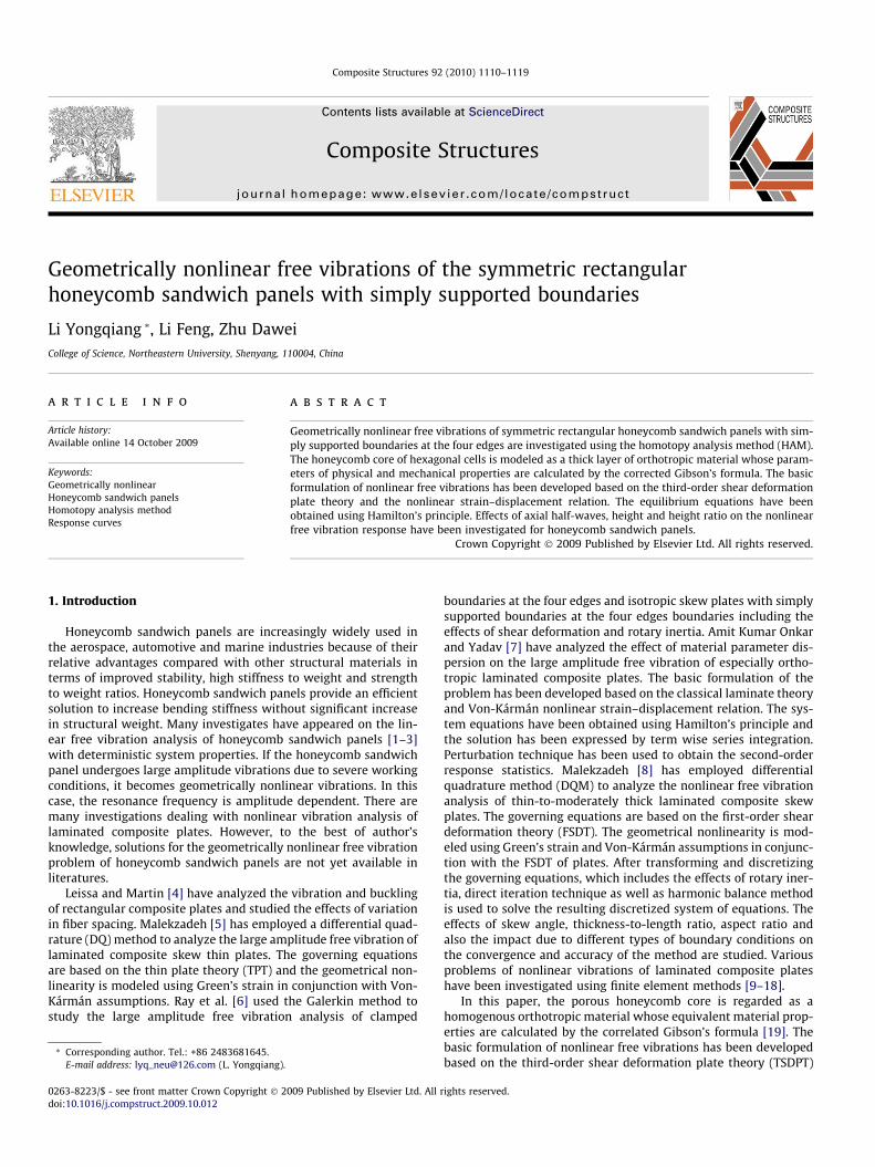
In this section, the governing differential equations of the non-linear free vibrations of symmetric rectangular honeycomb sand-wich panels with simply supported boundaries in terms of thedisplacements will be presented for the TSDPT. A typical honey-comb sandwich panel of length a, width b, height h and core heighthc is shown in Fig. 1, consists of two face sheets and arrays of opencells glued to the inner surfaces of the face sheets.

The displacement model assumed of the honeycomb sandwichpanel bases on the third-order shear deformation plate theory. Thedisplacements of a material point ðx; y; zÞ caused by bending maybe written as

u ¼ u0 þ zuxðx; y; tÞ � 4z3

3h2 uxðx; y; tÞ þ@wðx;y;tÞ

@x

� �v ¼ v0 þ zuyðx; y; tÞ � 4z3

3h2 uyðx; y; tÞ þ@wðx;y;tÞ

@y

� �w ¼ wðx; y; tÞ

8>>><>>>: ð1Þ

where u; v and w are the displacements along the x-, y- and z-direc-tions, respectively. u0; v0 and w0 are the mid-plane displacements.ux and uy are the rotations of normal to the mid-plane about the y-axis and x-axis, respectively.

From Green Lagrange strain vector, the nonlinear stain displace-ment relations are given as [28]

ex ¼@u@xþ 1

2@u@x

� �2

þ @v@x

� �2

þ @w@x

� �2" #

ey ¼@v@yþ 1

2@u@y

� �2

þ @v@y

� �2

þ @w@y

� �2" #

ez ¼ 0

cyz ¼@w@yþ @v@zþ @u@y

@u@zþ @v@y

@v@z

cxz ¼@w@xþ @u@zþ @u@x

@u@zþ @v@x

@v@z

cxy ¼@u@yþ @v@xþ @u@x

@u@yþ @v@x

@v@yþ @w@x

@w@y

ð2Þ

The stiffness and inertia parameters may be established byregarding honeycomb sandwich panel as a three layered laminatestructure. Under the assumption that each layer possesses a planeof elastic symmetry parallel to the x—y plane, the constitutiveequations for a layer can be written as

Fig. 1. Geometric configuration of a honeycomb sandwich panel.

rx

ry

ryz

rxz

rxy

8>>>>>><>>>>>>:

9>>>>>>=>>>>>>;¼

Q11 Q12 0 0 0Q21 Q22 0 0 0

0 0 Q 44 0 00 0 0 Q 55 00 0 0 0 Q 66

26666664

37777775

ex

ey

cyz

cxz

cxy

8>>>>>><>>>>>>:

9>>>>>>=>>>>>>;ð3Þ

Here we use the Hamilton’s principle to obtain the equilibriumequations which appropriates for the displacement field in Eq. (1)and constitutive equations in Eq. (3).

0 ¼ �Z t

0

Z h=2

�h=2

ZRðrxdex þ rydey þ rxydcxy þ ryzdcyz þ rxzdcxzÞdAdzdt

þ 12

dZ t

0

Z h=2

�h=2

ZRqð _u2 þ _v2 þ _w2ÞdAdzdt ð4Þ

Integrating the expressions in Eq. (4) by parts, and collecting thecoefficients of du; dv ; dw; dux and duy, we obtain the followingequilibrium equations of nonlinear free vibration of honeycombsandwich panels:

du0:

Nx;x þ Nxy;y þ@

@xNxu0

;x þ Nxyu0;y þ Mx �

4

3h2 Px

� �ux;x

�þ Mxy �

4

3h2 Pxy

� �ux;y þ Q x �

4

h2 Rx

� �ux �

4

3h2 Pxw;xx þ Pxyw;xy� �

� 4

h2 Rxw;x

þ @

@yNyu0

;y þ Nxyu0;x þ My �

4

3h2 Py

� �ux;y

�þ Mxy �

4

3h2 Pxy

� �ux;x þ Q y �

4

h2 Ry

� �ux �

4

3h2 Pyw;xy þ Pxyw;xx� �

� 4

h2 Ryw;x

¼ I1€u0 þ I2 �

4

3h2 I4

� �€ux �

4

3h2 I4 €w;x ð5aÞ

dv0:

Ny;y þ Nxy;x þ@

@xNxv0

;x þ Nxyv0;y þ Mx �

4

3h2 Px

� �uy;x

�þ Mxy �

4

3h2 Pxy

� �uy;y þ Qx �

4

h2 Rx

� �uy �

4

3h2 Pxw;xy þ Pxyw;yy� �

� 4

h2 Rxw;y

þ @

@yNyv0

;y þ Nxyv0;x þ My �

4

3h2 Py

� �uy;y

�þ Mxy �

4

3h2 Pxy

� �uy;x þ Qy �

4

h2 Ry

� �uy �

4

3h2 Pyw;yy þ Pxyw;xy� �

� 4

h2 Ryw;y

¼ I1 €v0 þ I2 �

4

3h2 I4

� �€uy �

4

3h2 I4 €w;y ð5bÞ

dw:

Qx;x þ Q y;y �4

h2 Rx;x þ Ry;y� �

þ 4

3h2 Px;xx þ Py;yy þ 2Pxy;xy� �

þ @

@xNxw;x þ Nxyw;y �

4

h2 Ryu0;y þ Rxu0

;x þ Xx �4

3h2 Yx

� �ux;x

�þ Xy �

4

3h2 Yy

� �ux;y

�þ 16

3h4 Yxw;xx þ Yyw;xy� �

þ @

@yNyw;y þ Nxyw;x �

4

h2 Rxv0;x þ Ryv0

;y þ Xx �4

3h2 Yx

� �uy;x

�þ Xy �

4

3h2 Yy

� �uy;y

�þ 16

3h4 Yxw;xy þ Yyw;yy� �

þ 4

3h2

@2

@x2 Pxu0;x þ Pxyu0

;y þ Tx �4

3h2 Kx

� �ux;x

�þ Txy �

4

3h2 Kxy

� �ux;y þ Xx �

4

h2 Yx

� �ux

� 4

3h2 Kxw;xx þ Kxyw;xy� �

� 4

h2 Yxw;x

1112 L. Yongqiang et al. / Composite Structures 92 (2010) 1110–1119

þ 4

3h2

@2

@y2 Pyv0;y þ Pxyv0

;x þ Ty �4

3h2 Ky

� �uy;y

�þ Txy �

4

3h2 Kxy

� �uy;x þ Xy �

4

h2 Yy

� �uy

� 4

3h2 Kyw;yy þ Kxyw;xy� �

� 4

h2 Yyw;y

þ 4

3h2

@2

@x@yPxv0

;x þ Pyu0;y þ Pxy u0

;x þ v0;y

� �þ Tx �

4

3h2 Kx

� �uy;x

�þ Ty �

4

3h2 Ky

� �ux;y þ Txy �

4

3h2 Kxy

� �ux;x þuy;y

� �þ Xx �

4

h2 Yx

� �uy þ Xy �

4

h2 Yy

� �ux

� 4

3h2 Kx þ Ky� �

w;xy þ Kxy w;xx þw;yy� ��

� 4

h2 Yxw;y þ Yyw;x� �

¼ I1 €w� 16

9h4 I7 €w;xx þ €w;yy� �

þ 4

3h2 I4 €u0;x þ €v0

;y

� �þ 4

3h2 I5 �4

3h2 I7

� �€ux;x þ €uy;y� �

ð5cÞ

dux:

Mx;x þMxy;y � Qx þ4

h2 Rx �4

3h2 Px;x þ Pxy;y� �

þ 4

3h2 Xx �4

h2 Yx

� �w;xx þ Xy �

4

h2 Yy

� �w;xy

�þ @

@xMx �

4

3h2 Px

� �u0;x þ Mxy �

4

3h2 Pxy

� �u0;y

�þ Sx �

8

3h2 Tx þ16

9h4 Kx

� �ux;x þ Sxy �

8

3h2 Txy þ16

9h4 Kxy

� �ux;y

þ Lx �16

3h2 Xx þ16

3h4 Yx

� �ux �

4

3h2 Tx �4

3h2 Kx

� �w;xx

þ Txy �

4

3h2 Kxy

� �w;xy

�� 4

h2 Xx �4

3h2 Yx

� �w;x

þ @

@yMy �

4

3h2 Py

� �u0;y þ Mxy �

4

3h2 Pxy

� �u0;x

�þ Sy �

8

3h2 Ty þ16

9h4 Ky

� �ux;y þ Sxy �

8

3h2 Txy þ16

9h4 Kxy

� �ux;x

þ Ly �16

3h2 Xy þ16

3h4 Yy

� �ux �

4

3h2 Ty �4

3h2 Ky

� �w;xy

þ Txy �

4

3h2 Kxy

� �w;xx

�� 4

h2 Xy �4

3h2 Yy

� �w;x

� Qx �

4

h2 Rx

� �u0;x � Q y �

4

h2 Ry

� �u0;y

� Lx �16

3h2 Xx þ16

3h4 Yx

� �ux;x � Ly �

16

3h2 Xy þ16

3h4 Yy

� �ux;y

¼ I3 �8

h2 I5 þ16

9h4 I7

� �€ux þ I2 �

4

3h2 I4

� �€u0

� 4

3h2 I5 �4

3h2 I7

� �€w;x ð5dÞ

duy:

My;y þMxy;x � Qy þ4

h2 Ry �4

3h2 Py;y þ Pxy;x� �

þ 4

3h2 Xx �4

h2 Yx

� �w;xy þ Xy �

4

h2 Yy

� �w;yy

�þ @

@xMx �

4

3h2 Px

� �v0;x þ Mxy �

4

3h2 Pxy

� �v0;y

�

þ Sx �8

3h2 Tx þ16

9h4 Kx

� �uy;x þ Sxy �

8

3h2 Txy þ16

9h4 Kxy

� �uy;y

þ Lx �16

3h2 Xx þ16

3h4 Yx

� �uy �

4

3h2 Tx �4

3h2 Kx

� �w;xy

þ Txy �

4

3h2 Kxy

� �w;yy

�� 4

h2 Xx �4

3h2 Yx

� �w;y

þ @

@yMy �

4

3h2 Py

� �v0;y þ Mxy �

4

3h2 Pxy

� �v0;x

�þ Sy �

8

3h2 Ty þ16

9h4 Ky

� �uy;y þ Sxy �

8

3h2 Txy þ16

9h4 Kxy

� �uy;x

þ Ly �16

3h2 Xy þ16

3h4 Yy

� �uy �

4

3h2 Ty �4

3h2 Ky

� �w;yy

þ Txy �

4

3h2 Kxy

� �w;xy

�� 4

h2 Xy �4

3h2 Yy

� �w;y

� Q x �

4

h2 Rx

� �v0;x � Qy �

4

h2 Ry

� �v0;y

� Lx �16

3h2 Xx þ16

3h4 Yx

� �uy;x � Ly �

16

3h2 Xy þ16

3h4 Yy

� �uy;y

¼ I3 �8

h2 I5 þ16

9h4 I7

� �€uy þ I2 �

4

3h2 I4

� �€v0

� 4

3h2 I5 �4

3h2 I7

� �€w;y ð5eÞ

These parameters appeared in Eq. (5) as follows:

ðNx;Ny;Nxy;Q x;QyÞ ¼Z h=2

�h=2ðrx;ry;rxy;rxz;ryzÞdz;

ðMx;My;Mxy; Lx; LyÞ ¼Z h=2

�h=2ðrx;ry;rxy;rxz;ryzÞzdz

ðSx; Sy; Sxy;Rx;RyÞ ¼Z h=2

�h=2ðrx;ry;rxy;rxz;ryzÞz2dz;

ðPx; Py; Pxy;Xx;XyÞ ¼Z h=2

�h=2ðrx;ry;rxy;rxz;ryzÞz3dz

ðTx; Ty; TxyÞ ¼Z h=2

�h=2ðrx;ry;rxyÞz4dz;

ðKx;Ky;KxyÞ ¼Z h=2

�h=2ðrx;ry;rxyÞz6dz;

ðYx; YyÞ ¼Z h=2

�h=2ðrxz;ryzÞz5dz

ðI1; I2; I3; I4; I5; I7Þ ¼Z h=2

�h=2qð1; z; z2; z3; z4; z6Þdz

ðAij;Bij;Dij; Eij; Fij;Gij;Hij; Jij;Kij;Mij;Nij; Pij;RijÞ

¼Z h=2

�h=2Q ijð1; z; z2; z3; z4; z5; z6; z7; z8; z9; z10; z11; z12Þdz

ði; j ¼ 1;2;6; 4;5Þ

For symmetric honeycomb sandwich panels, the following pa-nel parameter equals to zero:

Bij ¼ Eij ¼ Gij ¼ Jij ¼ Mij ¼ Pij ¼ I2 ¼ I4 ¼ 0 ð6Þ

For a rectangular honeycomb sandwich panel with simply sup-ported boundaries along all four edges (a and b are the plane-formdimensions of the panel; see Fig. 1), one solution for the flexuralvibration may be written as

L. Yongqiang et al. / Composite Structures 92 (2010) 1110–1119 1113

u0ðx; y; tÞ ¼P1

m;n¼1H1ðtÞ cos ax sin by

v0ðx; y; tÞ ¼P1

m;n¼1H2ðtÞ sin ax cos by

wðx; y; tÞ ¼P1

m;n¼1H3ðtÞ sin ax sin by

uxðx; y; tÞ ¼P1

m;n¼1H4ðtÞ cos ax sin by

uyðx; y; tÞ ¼P1

m;n¼1H5ðtÞ sinax cos by

8>>>>>>>>>>>>>>>>><>>>>>>>>>>>>>>>>>:

ð7Þ

where a ¼ mp=a; b ¼ np=b. m;n ¼ 1;2; . . . are the number of axialhalf-waves.

According to Eqs. (5) and (7), we obtain governing differentialequations for nonlinear free vibrations of symmetric rectangularhoneycomb sandwich panels with simply supported boundaries.The governing differential equations may be written as

€HNðtÞ þX5

k¼1

aN;kHkðtÞ þX5

k¼1

X5

p¼1

X5

q¼1

CN;k;p;qHkðtÞHpðtÞHqðtÞ ¼ 0;

N ¼ 1;2; . . . ;5 ð8Þ

where CN;k;p;q and aN;kðN; k;p; q ¼ 1;2; . . . ;5Þ are parameter relevantto I1; I2; I3; I4; I5; I7; Aij; Bij; Dijði; j ¼ 1;2;6; 4;5Þ, etc.

3. Basic idea of homotopy analysis method

Recently, an analytic method of nonlinear problems, called thehomotopy analysis method (HAM), has been developed by Liao[29]. Based on homotopy of topology, the validity of the HAM isindependent of whether or not there exists small parameters inthe considered equation. The HAM also avoids discretization andprovides an efficient numerical solution with high accuracy, mini-mal calculation, avoidance of physically unrealistic assumptions.Furthermore, the HAM always provides us with a family of solutionexpressions in the auxiliary parameter �h, the convergence regionand rate of each solution might be determined conveniently bythe auxiliary parameter �h [30].

In this section the basic idea of the HAM is introduced. To showthe basic idea, let us consider the following differential equation:

N½yðsÞ� ¼ 0;

where N is a nonlinear operator, s denote independent variables,yðsÞ is an unknown function, respectively. For simplicity, we ignoreall boundary or initial conditions, which can be treated in the sim-ilar way. More details about homotopy technique and its applica-tion are found in [20–27]. Liao [29] constructs the so-called zero-order deformation equation

ð1� qÞ‘½Uðs; qÞ � y0ðsÞ� ¼ q�hHðsÞN½Uðs; qÞ� ð9Þ

where q 2 ½0;1� is an embedding parameter, ‘ is an auxiliary linearoperator, Uðs; qÞ is an unknown function, y0ðsÞ is an initial guess ofyðsÞ; �h – 0 is a nonzero auxiliary parameter, HðsÞ is an auxiliaryfunction, respectively. It is important to note that, one has greatfreedom to choose auxiliary objects such as ‘ and �h in HAM. Obvi-ously, when q ¼ 0 and q ¼ 1, it holds

Uðs; 0Þ ¼ y0ðsÞ; Uðs; 1Þ ¼ yðsÞ;

respectively. Thus as q increases from 0 to 1, the solution Uðs; qÞvaries from the initial guess y0ðsÞ to the solution yðsÞ. ExpandingUðs; qÞ in Taylor series with respect to q, one has

Uðs; qÞ ¼ y0ðsÞ þXþ1M¼1

yMðsÞqM ð10Þ

where

yMðsÞ ¼1

M!

@MUðs; qÞ@qM

�����q¼0

ð11Þ

If the auxiliary linear operator, the initial guess, the auxiliaryparameter �h, and the auxiliary function HðsÞ are so properly cho-sen, the series (10) converges at q ¼ 1 and

Uðs; 1Þ ¼ y0ðsÞ þXþ1M¼1

yMðsÞ;

which must be one of solutions of the original nonlinear equation,as proved by Liao [29]. As �h = �1 and HðsÞ ¼ 1, Eq. (9) becomes

ð1� qÞ‘½Uðs; qÞ � y0ðsÞ� þ qN½Uðs; qÞ� ¼ 0; ð12Þ

which is used mostly in the homotopy-perturbation method [31].According to (11), the governing equation can be deduced from

the zeroth-order deformation Eq. (9). Define the vector

YM ¼ fy0ðsÞ; y1ðsÞ; . . . ; yMðsÞg

Differentiating (9) M times with respect to the embedding parame-ter q and then setting q ¼ 0 and finally dividing them by M!, wehave the so-called Mth-order deformation equation

‘½yMðsÞ � vMyM�1ðsÞ� ¼ �hHðsÞRMðYM�1Þ; ð13Þ

where

RMðYM�1Þ ¼1

M � 1ð Þ !@M�1N½Uðs; qÞ�

@qM�1

�����q¼0

ð14Þ

and

vM ¼0; M 6 11; M > 1

�It should be emphasized that yMðsÞðM P 1Þ is governed by the lin-ear Eq. (13) with the linear boundary conditions that come from theoriginal problem, which can be easily solved by symbolic computa-tion softwares such as Maple and Mathematica.

4. The solution with HAM

In order to solve Eq. (8) by HAM, defining the new variables

s ¼ xt; HNðtÞ ¼ uNðsÞ; N ¼ 1;2; . . . ;5 ð15Þ

where x is nonlinear frequency of honeycomb sandwich panels.Substituting Eq. (15) in Eq. (8), we obtain

x2€uNðsÞ þX5

k¼1

aN;kukðsÞ þX5

k¼1

X5

p¼1

X5

q¼1

CN;k;p;qukðsÞupðsÞuqðsÞ ¼ 0

N ¼ 1;2; . . . ;5 ð16Þ

To solve Eq. (16) by means of HAM, we choose a system of linearoperator

‘N ½UNðs; qÞ� ¼ x20@2UNðs; qÞ

@s2 þUNðs; qÞ" #

; N ¼ 1;2; . . . ;5 ð17Þ

with the property

‘N ½cN cosðsÞ� ¼ 0; N ¼ 1;2; . . . ;5 ð18Þ

where cN is constant. From Eq. (10), we define a system of nonlinearoperators as

1114 L. Yongqiang et al. / Composite Structures 92 (2010) 1110–1119

NN½U1ðs; qÞ;U2ðs; qÞ;U3ðs; qÞ;U4ðs; qÞ;U5ðs; qÞ;XðqÞ�

¼ X2ðqÞ€UNðs; qÞ þX5

k¼1

aN;kUkðsÞ þX5

k¼1

X5

p¼1

X5

q¼1

CN;k;p;qUkðs; qÞUp

� ðs; qÞUqðs; qÞ; N ¼ 1;2; . . . ;5 ð19Þ

where UNðs; qÞ is a kind of mapping of the unknown function uNðsÞ,and XðqÞ is a kind of mapping of unknown nonlinear frequency x.Using above the definition, we construct the zeroth-order deforma-tion equations

ð1� qÞ‘N½UNðs; qÞ � uN;0sÞ�¼ q�hHðsÞNN½U1ðs; qÞ;U2ðs; qÞ;U3ðs; qÞ;U4ðs; qÞ;U5ðs; qÞ;XðqÞ�;

N ¼ 1;2; . . . ;5 ð20Þ

where �h is a nonzero auxiliary parameter, HðsÞ is an auxiliary func-tion, uN;0ðsÞ is an initial guess of uNðsÞ, respectively.

The initial guess of uNðsÞcan be expressed by

uN;0ðsÞ ¼ AN;0 cosðsÞ; N ¼ 1;2; . . . ;5 ð21Þ

Obviously, when q ¼ 0 and q ¼ 1, it holds

UNðs; 0Þ ¼ uN;0ðsÞ; UNðs; 1Þ ¼ uNðsÞ; Xð0Þ ¼ x0;Xð1Þ ¼ x;N ¼ 1;2; . . . ;5 ð22Þ

respectively. Thus, as q increases from 0 to 1, the solution UNðs; qÞvaries from the initial guess uN;0ðsÞ to the solution uNðsÞ of Eq.(16), for N ¼ 1;2; . . . ;5, respectively. Likewise, XðqÞ varies fromthe initial guess x0 to the unknown frequency x.

Expanding UNðs; qÞ and XðqÞ in Taylor series with respect toq,for N ¼ 1;2; . . . ;5, we have

UNðs; qÞ ¼ uN;0ðsÞ þXþ1M¼1

uN;MðsÞqM ; ð23Þ

XðqÞ ¼ x0 þXþ1M¼1

xMqM; ð24Þ

where

uN;MðsÞ ¼1

M!:@MUNðs; qÞ

@qMjq¼0 ð25Þ

xM ¼1

M!:@MXðqÞ@qM jq¼0 ð26Þ

If the auxiliary parameter �h and the auxiliary function HðsÞ areproperly chosen, the above series converge when q ¼ 1, then wehave

uNðsÞ ¼ uN;0ðsÞ þXþ1M¼1

uN;MðsÞ; N ¼ 1;2; . . . ;5 ð27Þ

x ¼ x0 þXþ1M¼1

xM; ð28Þ

which must be one of solutions of the original nonlinear equations,as proved by Liao [29].

Defining the vector

eUM ¼ fU1;M;U2;M;U3;M ;U4;M;U5;Mg;eXM ¼ fx0;x1;x2; . . . ;xMg M ¼ 0;1;2; . . . ;1 ð29Þ

where

UN;M ¼ fuN;0ðsÞ;uN;1ðsÞ;uN;2ðsÞ; . . . ;uN;MðsÞg; N ¼ 1;2; . . . ;5:

Differentiating the zero-order deformation Eq. (20) M times with re-spect to the embedding parameter q, setting q ¼ 0 and finally divid-

ing them by M!, we have the so-called Mth-order deformationequation

‘N ½uN;MðsÞ � vN;MuN;M�1ðsÞ� ¼ �hHðsÞRN;MðeUM�1; eXM�1Þ;N ¼ 1;2; . . . ;5; M ¼ 1;2; . . . ;1 ð30Þ

where

RN;MðeUM�1; eXM�1Þ ¼1

ðM � 1Þ!

� dM�1NN½U1ðs; qÞ;U2ðs; qÞ;U3ðs; qÞ;U4ðs; qÞ;U5ðs; qÞ;XðqÞ�dqM�1 jq¼0

¼XM�1

i¼0

Xi

j¼0

xjxi�j€uN;M�1�iðsÞ þX5

k¼1

½aN;kuk;M�1ðsÞ�

þX5

k¼1

X5

p¼1

X5

q¼1

CN;k;p;q

XM�1

i¼0

Xi

j¼0

Xi�j

r¼0

uk;jðsÞup;rðsÞuq;i�j�rðsÞ;

N ¼ 1;2; . . . ;5; M ¼ 1;2; . . . ;1 ð31Þand

vN;M ¼0; M 6 1;1; M > 1:

�N ¼ 1;2; . . . ;5; M ¼ 1;2; . . . ;1 ð32Þ

In order to obey the rule of solution expression and the rule ofthe coefficient ergodicity [29], the corresponding auxiliary functioncan be determined uniquely

HðsÞ ¼ 1 ð33Þ

It is found that the Eq. (31) contains the so-called secular term.Eq. (31) is expressed by

RN;MðeUM�1; eXM�1Þ¼ gN;0ðA1;0;A2;0;A3;0;A4;0;A5;0; eXM�1Þ cosðsÞ

þXKM

k¼1

gN;kðA1;0;A2;0;A3;0;A4;0;A5;0; eXM�1Þ cos½gks�;

N ¼ 1;2; . . . ;5; M ¼ 1;2; . . . ;1 ð34Þwhere KM is a positive integer dependent on the order M. gk is a realbut gk – 1(do not equal 1). To avoid the secular terms, we must en-force the coefficient of cos(s) equal zero

gN;0ðA1;0;A2;0;A3;0;A4;0;A5;0; eXM�1Þ ¼ 0; N ¼ 1;2; . . . ;5;

M ¼ 1;2; . . . ;1 ð35Þ

then obtain a group of algebraic equations for A1;0; A2;0; A3;0; A4;0;

A5;0 and xM�1.After A1;0; A2;0; A3;0; A4;0; A5;0 and xM�1 solved, uN;MðsÞ can be

solved from Mth-order deformation Eq. (30). It has been provedthat, as long as the series of solution given by the homotopy anal-ysis method converges, it must be one of exact solutions. Note thatthe series of solution (27) and (28) contain the auxiliary parameter�h, which provides us with a simple way to adjust and control theconvergence of the series solution. In general, by means of theso-called �h-curve, as pointed by Liao [29], the valid region of �h isa horizontal line segment. We can plot the �h-curve ofA1;0; A2;0; A3;0; A4;0; A5;0 and determine the valid region of �h.

In order to explain the x and uNðsÞ specific solution process, thefollowing M ¼ 1 as an example to explain. When M ¼ 1, accordingto Eq. (31), we obtain

RN;1ðeU0; eX0Þ

¼ x20€uN;0ðsÞ þ

X5

k¼1

½aN;kuk;0ðsÞ�

þX5

k¼1

X5

p¼1

X5

q¼1

CN;k;p;quk;0ðsÞup;0ðsÞuq;0ðsÞ; N ¼ 1;2; . . . ;5

ð36Þ

L. Yongqiang et al. / Composite Structures 92 (2010) 1110–1119 1115

Substituting Eq. (21) in Eq. (36)

RN;1ðeU0; eX0Þ

¼ �x20AN;0 þ

X5

k¼1

aN;kAk;0 þ34

X5

k¼1

X5

p¼1

X5

q¼1

CN;k;p;qAk;0Ap;0Aq;0

( )

� cosðsÞ þ 14

X5

k¼1

X5

p¼1

X5

q¼1

CN;k;p;qAk;0Ap;0Aq;0 cosð3sÞ;

N ¼ 1;2; . . . ;5 ð37Þ

To avoid the secular terms, we must enforce the coefficient ofcos(s) of Eq. (37) equal zero, then Eq. (35) is expressed by,

gN;0ðA1;0;A2;0;A3;0;A4;0;A5;0;x0Þ

¼ �x20AN;0 þ

X5

k¼1

aN;kAk;0 þ34

X5

k¼1

X5

p¼1

X5

q¼1

CN;k;p;qAk;0Ap;0Aq;0 ¼ 0;

N ¼ 1;2; . . . ;5 ð38Þ

A1;0; A2;0; A3;0; A4;0; A5;0 and x0 relations can be solved from Eq.(38). Then, Eq. (30) become

€uN;1ðsÞ þ uN;1ðsÞ ¼�h

4x20

X5

k¼1

X5

p¼1

X5

q¼1

CN;k;p;qAk;0Ap;0Aq;0 cosð3sÞ;

N ¼ 1;2; . . . ;5:

u1;1; u2;1; u3;1; u4;1 and u5;1 can be solved.

-3 -2 -1 0 1 2-5

-4

-3

-2

-1

0

1

2

3

4

5

A1,

0, A

2,0

A1.0

A2.0

h

Fig. 2. �h-Curve of A1;0 and A2;0 given by sixth-order approximation.

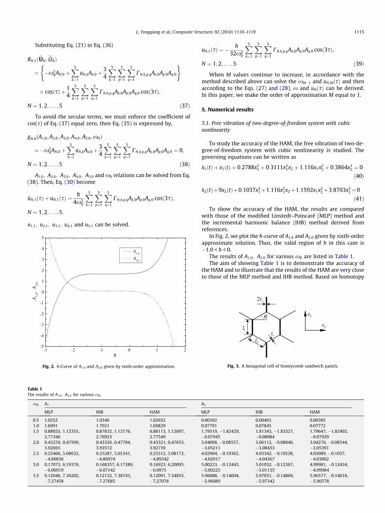
Table 1The results of A1;0 ; A2;0 for various x0.

x0 A1

MLP IHB HAM

0.5 1.0252 1.0346 1.026521.0 1.6991 1.7021 1.698291.5 0.88025, 1.12355,

2.773460.87832, 1.12176,2.76923

0.88113, 1.12697,2.77549

2.0 0.43259, 0.47599,3.92693

0.43326, 0.47704,3.93572

0.43321, 0.47653,3.92739

2.5 0.25466, 5.08632,�4.89836

0.25287, 5.05341,�4.86974

0.25512, 5.08173,�4.89342

3.0 0.17073, 6.19376,�6.06919

0.168357, 6.17389,�6.07142

0.16923, 6.20095,�6.0975

3.5 0.12046, 7.36202,�7.27458

0.12132, 7.38193,�7.27685

0.12091, 7.34855,�7.27078

uN;1ðsÞ ¼ ��h

32x20

X5

k¼1

X5

p¼1

X5

q¼1

CN;k;p;qAk;0Ap;0Aq;0 cosð3sÞ;

N ¼ 1;2; . . . ;5 ð39Þ

When M values continue to increase, in accordance with themethod described above can solve the xM�1 and uN;MðsÞ and thenaccording to the Eqs. (27) and (28), x and uNðsÞ can be derived.In this paper, we make the order of approximation M equal to 1.

5. Numerical results

5.1. Free vibration of two-degree-of-freedom system with cubicnonlinearity

To study the accuracy of the HAM, the free vibration of two-de-gree-of-freedom system with cubic nonlinearity is studied. Thegoverning equations can be written as

€x1ðtÞ þ x1ðtÞ þ 0:2788x31 þ 0:3111x2

1x2 þ 1:116x1x22 þ 0:3864x3

2 ¼ 0

ð40Þ

€x2ðtÞþ9x2ðtÞþ0:1037x31þ1:116x2

1x2þ1:1592x1x22þ3:8703x3

2¼0

ð41Þ

To show the accuracy of the HAM, the results are comparedwith those of the modified Linstedt–Poincaré (MLP) method andthe incremental harmonic balance (IHB) method derived fromreferences.

In Fig. 2, we plot the �h-curve of A1;0 and A2;0 given by sixth-orderapproximate solution. Thus, the valid region of �h in this case is�1.0 < �h < 0.

The results of A1;0; A2;0 for various x0 are listed in Table 1.The aim of showing Table 1 is to demonstrate the accuracy of

the HAM and to illustrate that the results of the HAM are very closeto those of the MLP method and IHB method. Based on homotopy

ct2

ct1l

2l

cθ 2x

1x

Fig. 3. A hexagonal cell of honeycomb sandwich panels.

A2

MLP IHB HAM

0.00392 0.00403 0.003850.07791 0.07845 0.077721.79519, �1.82429,�0.07945

1.81343, �1.83327,�0.08084

1.79647, �1.82492,�0.07929

3.04098, �0.08557,�3.05211

3.06112, �0.08846,�3.08433

3.04276, �0.08544,�3.05391

4.02904, �0.10362,�4.02917

4.03342, �0.10538,�4.04367

4.03089, �0.1037,�4.03002

5.00223, �0.12443,�5.00225

5.01032, �0.12367,�5.01135

4.99981, �0.12434,�4.99984

5.96088, �0.14604,�5.96089

5.97031, �0.14869,�5.97342

5.96577, �0.14618,�5.96578

1116 L. Yongqiang et al. / Composite Structures 92 (2010) 1110–1119

in topology, the validity of the HAM is independent of whether ornot there exist small parameters in the considered equation. TheHAM always provides us with a family of solution expressions inthe auxiliary parameter �h, and the convergence region and rateof each solution might be determined conveniently by the auxiliaryparameter �h. This method has been successfully applied to solvemany types of nonlinear problems in engineering and science.Therefore, the HAM is suitable for free vibration of multi-degree-of-freedom system with strongly nonlinearity.

0 20000 40000 60000 80000 100000-2.5

-2.0

-1.5

-1.0

-0.5

0.0

0.5

1.0

1.5

2.0

2.5

ω0 , rad/s

m=1,n=1

A1.

0

0 20000 40000 60000 80000 100000-3.0

-2.5

-2.0

-1.5

-1.0

-0.5

0.0

0.5

1.0

1.5

2.0

2.5

3.0

ω0 , rad/s

m=1,n=1

A3.

0

0 20000 40000-15000

-10000

-5000

0

5000

10000

15000

ω0 , r

m=1,n=1

A5.

0

Fig. 4. Nonlinear free vibration response A1;0—x0; A2;0—x0; A3;0—x0

5.2. Nonlinear free vibration of symmetric rectangular honeycombsandwich panels with simply supported boundaries

In this section, nonlinear free vibration of symmetric rectangu-lar honeycomb sandwich panels with simply supported boundariesis studied. The square panels contain two aluminum face sheets,and an aluminum core of hexagonal cells illustrated in Fig. 3. Thestructural details of the panels and core are given here:a ¼ b ¼ 1 m; l1 ¼ l2 ¼ 1:833 mm; tc ¼ 0:0254 mm; hc ¼ 300. The

0 20000 40000 60000 80000 100000-2.5

-2.0

-1.5

-1.0

-0.5

0.0

0.5

1.0

1.5

2.0

2.5

ω0 , rad/s

m=1,n=1

A2.

0

0 20000 40000 60000 80000 100000-10000

-8000

-6000

-4000

-2000

0

2000

4000

6000

8000

10000

ω0 , rad/s

m=1,n=1

A4.

0

60000 80000 100000

ad/s

; A4;0—x0 and A5;0—x0 for h ¼ 0:1 m; hc=h ¼ 0:95; m ¼ 1; n ¼ 1.

L. Yongqiang et al. / Composite Structures 92 (2010) 1110–1119 1117

material properties of the panels and core are given byE ¼ 69 GPa; t ¼ 0:3; q ¼ 2700 kg=m3; G ¼ E=2ð1þ tÞ. The panelthicknesses are allowed to vary between 0.05 and 0.1 m. hc=h areallowed to vary between 0.85 and 0.95. The equivalent core prop-erties were calculated by the corrected Gibson’s formula [19].

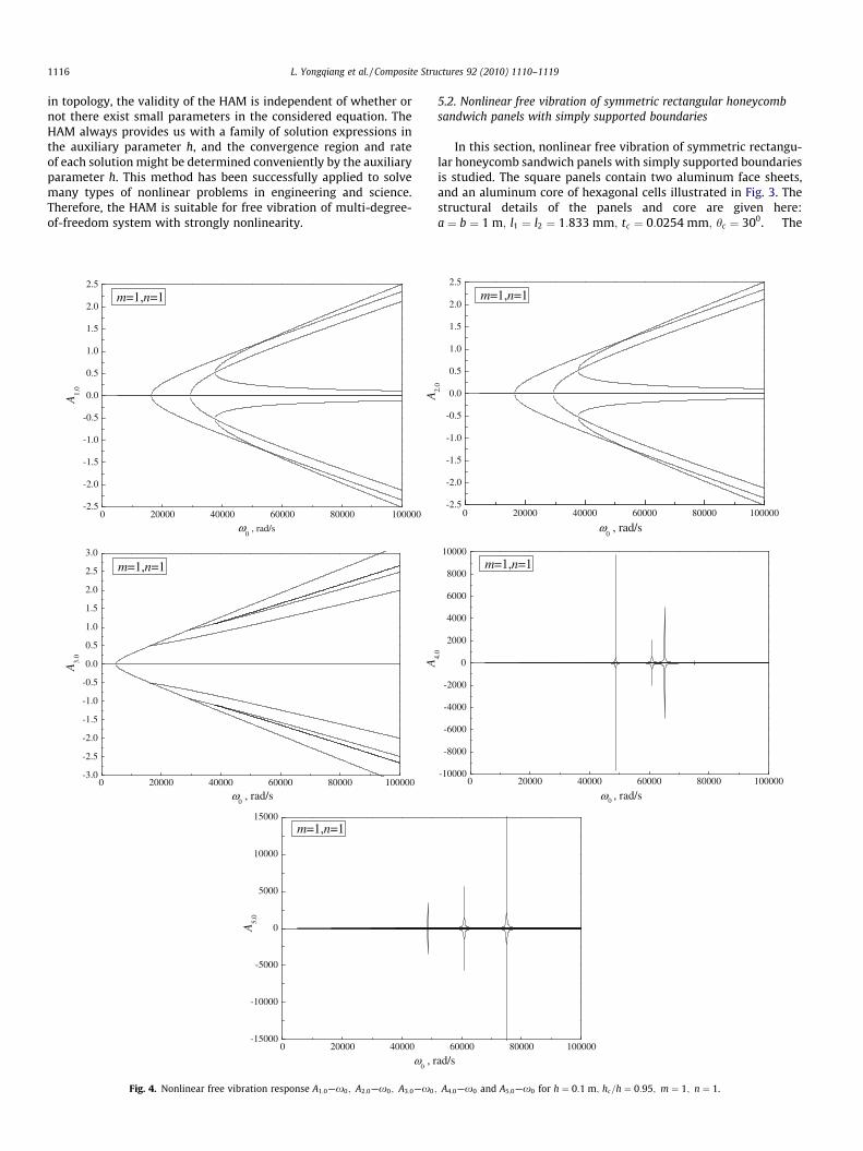
Fig. 4 shows the response curves A1;0—x0; A2;0—x0; A3;0—x0;

A4;0—x0 and A5;0—x0 for h ¼ 0:1 m; hc=h ¼ 0:95; m ¼ 1 and n ¼ 1.When h ¼ 0:1; hc=h ¼ 0:95; m ¼ 1; n ¼ 1, the honeycomb

sandwich panel of five natural frequencies are 3141.93, 11750.2,20440.96, 30438.95 and 37846.54 rad/s. From the curve ofA1;0—x0 and A2;0—x0in Fig. 4, it can be seen that the bifurcation oc-

30000 40000 50000 60000 70000 80000 90000 100000

-0.4

-0.2

0.0

0.2

0.4h=0.1m, hc/h=0.85, m=2, n=2

h=0.05m, hc/h=0.85, m=2, n=2

ω0 , rad/s

A1.

0

0 20000 40000 60000 80000 100000-0.8

-0.6

-0.4

-0.2

0.0

0.2

0.4

0.6

0.8

ω0 , rad/s

A3.

0

h=0.1m, hc/h=0.85, m=2, n=2

h=0.05m, hc/h=0.85, m=2, n=2

A

60000 70000 800-5000

-2500

0

2500

5000h=0.1m, hc/h=0.85, m=2, n=2

h=0.05m, hc/h=0.85, m=2, n=2

ω0 , ra

A5.

0

Fig. 5. Nonlinear free vibration response A1;0—x0; A2;0—x0; A3;0

curs when A1;0 and A2;0 separate at the point x0 equal 16,400,29,400 and 37,700 rad/s. These two frequencies 16,400 and29,400 rad/s are nearly 1.5 times the corresponding natural fre-quencies 11750.2 and 20440.96 rad/s; the frequency 37,700 rad/sis nearly 1 times the corresponding natural frequencies37846.54 rad/s. The bifurcation not only occurs when A3;0 at thepoint x0 which is equal to 16,400, 29,400 and 37,700 rad/s, it alsooccurs at 4800 rad/s which is 1.5 times the natural frequency3141.93 rad/s.

From the curve of A4;0—x0 in Fig. 4, it can be seen that the res-onance will occurs when x0 equal 48,700, 60,900, 65,200 and

30000 40000 50000 60000 70000 80000 90000 100000

-0.4

-0.2

0.0

0.2

0.4h=0.1m, hc/h=0.85, m=2, n=2

h=0.05m, hc/h=0.85, m=2, n=2

ω0 , rad/s

A2.

0

60000 80000 100000-3000

-2000

-1000

0

1000

2000

3000h=0.1m, hc/h=0.85, m=2, n=2

h=0.05m, hc/h=0.85, m=2, n=2

ω0 , rad/s

4.0

00 90000 100000

d/s

—x0; A4;0—x0 and A5;0—x0 for hc=h ¼ 0:85; m ¼ 2; n ¼ 2.

1118 L. Yongqiang et al. / Composite Structures 92 (2010) 1110–1119

75,100 rad/s. These two frequencies 48,700 and 60,900 rad/s isnearly 1.5 times the corresponding natural frequencies 30438.95and 37846.54 rad/s; the frequency 65,200 rad/s is nearly 3 timesthe corresponding natural frequencies 20440.96 rad/s; the fre-quency 75,100 rad/s is nearly 2 times the corresponding naturalfrequencies 37846.54 rad/s. From the curve of A5;0—x0 in Fig. 4,it can be seen that the resonance occurs when x0 equal 48,700,60,900 and 75,100 rad/s. It can be seen in Fig. 4 that the structure

0 20000 40000 60000 80000 100000-2.5

-2.0

-1.5

-1.0

-0.5

0.0

0.5

1.0

1.5

2.0

2.5hc/h=0.95, h=0.05m, m=1, n=1

hc/h=0.85, h=0.05m, m=1, n=1

ω0 , rad/s

A1.

0

A

0 20000 40000 60000 80000 100000-3.0

-2.5

-2.0

-1.5

-1.0

-0.5

0.0

0.5

1.0

1.5

2.0

2.5

3.0hc/h=0.95, h=0.05m, m=1, n=1

hc/h=0.85, h=0.05m, m=1, n=1

ω0 , rad/s

A3.

0

A

60000 70000 80-3000

-2000

-1000

0

1000

2000

3000h

c/h=0.95, h=0.05m, m=1, n=1

hc/h=0.85, h=0.05m, m=1, n=1

ω0 , r

A 5.0

Fig. 6. Nonlinear free vibration response A1;0—x0; A2;0—x0; A3

emergence the bifurcation or resonance in the 1.5 times of naturalfrequency.

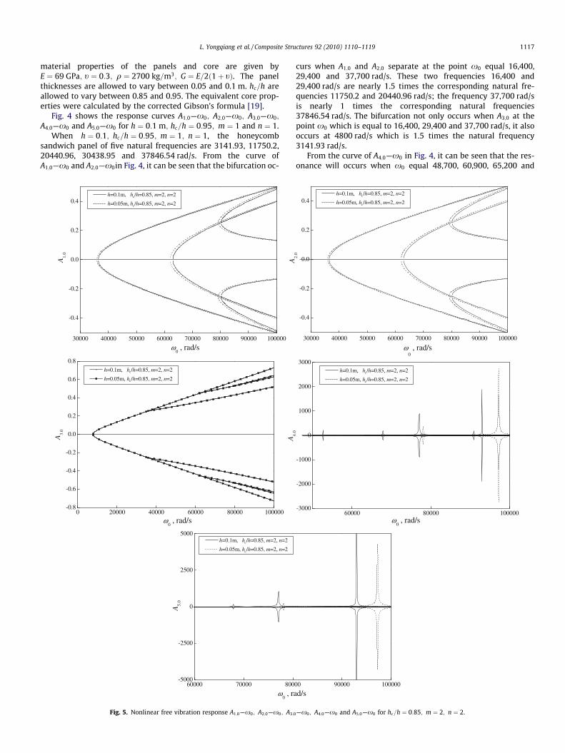
The effects of height on the nonlinear free vibration response ofhoneycomb sandwich panels are examined for different height h.Fig. 5 show the response curves when hc=h ¼ 0:85; m ¼ 2; n ¼ 2,and h equals to 0.05 m and 0.1 m respectively.

It can be seen in Fig. 5 that the values of A1;0 and A2;0 in thebifurcation pot increase with the value of h increased, A3;0 does

0 20000 40000 60000 80000 100000-2.5

-2.0

-1.5

-1.0

-0.5

0.0

0.5

1.0

1.5

2.0

2.5hc/h=0.95, h=0.05m, m=1, n=1

hc/h=0.85, h=0.05m, m=1, n=1

ω0 , rad/s

2.0

60000 70000 80000 90000 100000-9000

-6000

-3000

0

3000

6000

9000hc/h=0.95, h=0.05m, m=1, n=1

hc/h=0.85, h=0.05m, m=1, n=1

ω0 , rad/s

4.0

000 90000 100000

ad/s

;0—x0; A4;0—x0 and A5;0—x0 for h ¼ 0:05 m; m ¼ 1; n ¼ 1.

L. Yongqiang et al. / Composite Structures 92 (2010) 1110–1119 1119

not change basically, which indicates that the change of h impactlittle on the A3;0 with the value of h increased, whereas the valuesof A4;0 and A5;0 in the resonance pot reduce with the value of hincreased.

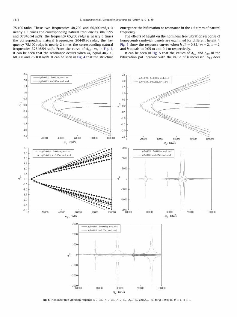
The effects of height ratio hc=h on the nonlinear free vibrationresponse of honeycomb sandwich panels are examined. Fig. 6 showthe response curves when h ¼ 0:05 m; m ¼ 1; n ¼ 1, and hc=hequals to 0.85 and 0.95 respectively.

It can be seen in Fig. 6 that the values of A1;0 and A2;0 in thebifurcation pot reduce with the value of hc=h increased, the valueof A3;0 in the bifurcation pot does not change basically, but theamplitude increases with the value of hc=h increased, and the val-ues of A4;0 and A5;0 in the resonance pot increase with the value ofhc=h increased.

6. Conclusions

Geometrically nonlinear free vibrations of symmetric rectangu-lar honeycomb sandwich panels with simply supported boundariesat the four edges are investigated using the homotopy analysismethod The basic formulation of nonlinear free vibrations has beendeveloped based on the third-order shear deformation plate theoryand the nonlinear strain–displacement relation. The parameters ofmechanical properties are determined by the corrected Gibson’sformula. Numerical results have been presented for the free vibra-tion analysis of honeycomb sandwich panels having different axialhalf-waves, height and height ratio. It is observed that the struc-ture emergence the bifurcation or resonance in the 1, 1.5, 2 and3 times of natural frequency.

The values of A1;0 and A2;0 in the bifurcation pot increase withthe value of h increased. A3;0 does not change basically and the val-ues of A4;0; A5;0 in the resonance pot reduce with the value of h in-creased. The values of A1;0; A2;0 in the bifurcation pot reduce withthe value of hc=h increased, the value of A3;0 in the bifurcation potdoes not change basically, but the amplitude increases with the va-lue of hc=h increased, and the values of A4;0 and A5;0 in the reso-nance pot increase with the value of hc=h increased.

References

[1] Yu SD, Cleghorn WL. Free flexural vibration analysis of symmetric honeycombpanels. J Sound Vib 2005;284(1):189–204.

[2] Yongqiang Li, Zhiqiang Jin. Free flexural vibration analysis of symmetricrectangular honeycomb panels with SCSC edge supports. Compos Struct2008;83(2):154–8.

[3] Yongqiang L, Dawei Z. Free flexural vibration analysis of symmetricrectangular honeycomb. Compos Struct 2009;88(1):33–9.

[4] Leissa AW, Martin AF. Vibration buckling of rectangular composite plates withvariable fiber spacing. Compos Struct 1990;14(4):339–57.

[5] Malekzadeh P. A differential quadrature nonlinear free vibration analysis oflaminated composite skew thin plates. Thin-Wal Struct 2007;45(2):237–50.

[6] Ray AK, Banerjee B, Bhattacharjee B. Large amplitude free vibrations of skewplates including transverse shear deformation and rotary inertia – a newapproach. J Sound Vib 1995;180(4):669–81.

[7] Onkar AK, Yadav D. Non-linear free vibration of laminated composite platewith random material properties. J Sound Vib 2004;272(3–5):627–41.

[8] Malekzadeh P. Differential quadrature large amplitude free vibration analysisof laminated skew plates based on FSDT. Compos Struct 2008;83(2):189–200.

[9] Ganapathi M, Varadan TK, Sarma BS. Nonlinear flexural vibrations of laminatedorthotropic plates. Compos Struct 1991;39(6):685–8.

[10] Sivakumar K, Iyengar NGR, Deb K. Free vibration of laminated composite plateswith cutouts. J Sound Vib 1999;221(3):443–70.

[11] Singha MK, Ganapathi M. Large amplitude free flexural vibrations of laminatedcomposite skew plates. Int J Non-Linear Mech 2004;39(10):1709–20.

[12] Sundararajana N, Prakash T, Ganapathi M. Nonlinear free flexural vibrations offunctionally graded rectangular and skew plates under thermal environments.Finite Elements Anal Des 2005;42(2):152–68.

[13] Attia O, El-Zafrany A. A high-order shear element for nonlinear vibrationanalysis of composite layered plates and shells. Int J Mech Sci1999;41(4):461–86.

[14] Singha MK, Rupesh D. Nonlinear vibration of symmetrically laminatedcomposite skewplates by finite element method. Int J Non-Linear Mech2007;42(9):1144–52.

[15] Kim TW, Kim JH. Nonlinear vibration of viscoelastic laminated compositeplates. Int J Solids Struct 2002;39(10):2857–70.

[16] Argyris J, Tenek L, Olofsson L. Nonlinear free vibrations of composite plates.Comput Methods Appl Mech Eng 1994;115(1):1–51.

[17] Naidu NVS, Sinha PK. Nonlinear free vibration analysis of laminated compositeshells in hygrothermal environments. Compos Struct 2007;77(4):475–83.

[18] Lal A, Singh BN, Kumar R. Nonlinear free vibration of laminated compositeplates on elastic foundation with random system. Int J Mech Sci2008;50(7):1203–12.

[19] Fu MH, Yin JR. Equivalent elastic parameters of the honeycomb core. ActaMech Sin 1999;31(1):113–8.

[20] Liao SJ. A new branch of solutions of boundary-layer flows over animpermeable stretched plate. Int J Heat Mass Transfer 2005;48(12):2529–39.

[21] Liao SJ. An explicit, totally analytic solution of laminar viscous flow over asemi-infinite flat plate. Commun Nonlinear Sci Numer Simulat1998;3(2):53–7.

[22] Liao SJ. An analytic solution of unsteady boundary-layer flows caused by animpulsively stretching plate. Commun Nonlinear Sci Numer Simulat2006;11(3):326–39.

[23] Liao SJ. An approximate solution technique which does not depend upon smallparameters: a special example. Int J Non-Linear Mech 1995;30(3):371–80.

[24] Liao SJ. An approximate solution technique which does not depend upon smallparameters (Part 2): an application in fluid mechanics. Int J Non-Linear Mech1997;32(5):815–22.

[25] Wen JM, Cao ZC. Sub-harmonic resonances of nonlinear oscillations withparametric excitation by means of the homotopy analysis method. Phys Lett A2007;371(5):427–31.

[26] Tan Y, Abbasbandy S. Homotopy analysis method for quadratic Riccatidifferential equation. Commun Nonlinear Sci Numer Simulat2008;13(3):539–46.

[27] Abbasbandy S. Approximate solution for the nonlinear model of diffusion andreaction in porous catalysts by means of the homotopy analysis method. ChemEng J 2008;136(2):144–50.

[28] Chia CY. Nonlinear analysis of plates. New York: McGraw-Hill; 1980.[29] Liao SJ. Beyond perturbation: introduction to the homotopy analysis

method. Boca Raton: Chapman & Hall; 2003.[30] Rashidi MM, Domairry G, Dinarvand S. Approximate solutions for the Burger

and regularized long wave equations by means of the homotopy analysismethod. Commun Nonlinear Sci Numer Simulat 2009;14(3):708–17.

[31] He JH. Homotopy perturbation method: a new nonlinear analytical technique.Appl Math Computat 2003;135(1):73–9.