Geometry Modeling And Visualisation

Using SciPy And pythonOCC r0.10

Reinhard Jansohn

May 3, 2010

Abstract

The results of computations in 3D cannot be drawn easily on a two dimensional medium like paper.As a consequence mathematical books and introductional texts dealing with that often do not offermany figures which help students gaining an imagination of the meaning of all the formulas. Theremedy is the application of a mathematical software combined with the visualization capabilitiesof a 3D modelling software. Python [2] offers both maths (Scipy [7]) and visualization capabilities(pythonOCC [3]). In addition Python may be learned in a few days. This document shows how tovisualise geometric computations performed with SciPy in pythonOCC.

For SciPy the documentation and other sources on the web provide a huge amount of informa-tion. But how to create visualizations with the aid of pythonOCC? Looking for information aboutthat will give you less extensive documents1. This little paper may help you to get started creatingvisualizations utilising pythonOCC more painlessly.

After reading and trying the step by step examples you should be able to write your code simplyby steeling snippets from the examples delivered with pythonOCC.

Acknowledgement

This little booklet would not exist without the support of Thomas Paviot. I also like to thank alldevelopers of Open Cascade and pythonOCC for their great work.

1This is only true for the actual version 0.4 of pythonOCC at time of writing.

License

This document is distributed under the terms of the Creative Common BY-NCSA 3.0 li-cense. In a few words:

You are free:

• to Share

• to copy, distribute and transmit the work to Remix

• to adapt the work

Under the following conditions:

• Attribution — You must attribute the work in the manner specified by the author orlicensor (but not in any way that suggests that they endorse you or your use of thework).

• Noncommercial — You may not use this work for commercial purposes.

• Share Alike — If you alter, transform, or build upon this work, you may distributethe resulting work only under the same or similar license to this one.

With the understanding that:

• Waiver –— Any of the above conditions can be waived if you get permission from thecopyright holder.

• Public Domain –— Where the work or any of its elements is in the public domainunder applicable law, that status is in no way affected by the license.

• Other Rights —– In no way are any of the following rights affected by the license:

– Your fair dealing or fair use rights, or other applicable copyright exceptions andlimitations;

– The author’s moral rights;

– Rights other persons may have either in the work itself or in how the work isused, such as publicity or privacy rights.

• Notice — For any reuse or distribution, you must make clear to others the licenseterms of this work. The best way to do this is with a link to this2 web page.

2http://creativecommons.org/licenses/by-nc-sa/3.0/

2

Contents

1 Step 1 - The frame 4

2 Step 2 - Drawing Spheres 6

2.1 Drawing spheres from points . . . . . . . . . . . . . . . . . . . . . . . . . . . . 6

2.2 Drawing spheres from Scipy arrays . . . . . . . . . . . . . . . . . . . . . . . . . 9

3 Step 3 - Boolean Operations 11

3.1 What are Boolean Operations? . . . . . . . . . . . . . . . . . . . . . . . . . . . . 11

3.2 A first sample on Boolean operations in pythonOCC . . . . . . . . . . . . . . . 12

3.3 Extending the first sample on Boolean operations in pythonOCC . . . . . . . 14

3.3.1 What we want to do and how it looks like . . . . . . . . . . . . . . . . . 14

3.3.2 Creating a cylinder . . . . . . . . . . . . . . . . . . . . . . . . . . . . . . 15

3.3.3 Creating a cone . . . . . . . . . . . . . . . . . . . . . . . . . . . . . . . . 19

3.3.4 Creating an arrow . . . . . . . . . . . . . . . . . . . . . . . . . . . . . . 20

4 Step 4 - Time for Practice 24

4.1 Extending our sample . . . . . . . . . . . . . . . . . . . . . . . . . . . . . . . . 24

4.2 Time for Housekeeping . . . . . . . . . . . . . . . . . . . . . . . . . . . . . . . . 27

4.3 Once more: Extending the sample . . . . . . . . . . . . . . . . . . . . . . . . . 28

A Advanced GUI programming utilizing wx.PySimpleApp 32

B History of this document 34

3

1 Step 1 - The frame

Our first step is to provide a frame which is used in the next steps. This frame consists ofa menu where we can hook functions to be selected and a canvas where all our drawingswill be displayed.

Read and run Step1.py (see listing 1 given below) 3.

Figure 1 shows what you should get if you execute Step1.py. If you installed allwhat’s needed you should see our empty pythonOCC screen. Please study the code and thecomments added. If you have questions don’t worry. The comments in the code providemore information than needed for following this step by step course. If you just acceptthe code as it is and try to figure out how to get something similar done that’s fine for themoment.

It is interesting to note that there is no import of a GUI-framework like import wx inthe code. All the GUI stuff is found in OCC.Display.SimpleGui. In that module theenvironment is examined and the approprate GUI framework is initalized. So if you like toknow what is going on behind the scene have a look at OCC.Display.SimpleGui4.

Figure 1: Screenshot of Step1

3In the following sections only the relevant parts of the code is presented in the script. If you are not surehow this code fits into the program please read the example code listing.

4If you make use of wxPython you can also use the sample given in Appendix A. Here a sample of theappilcation of the class wx.PySimpleApp is given.

4

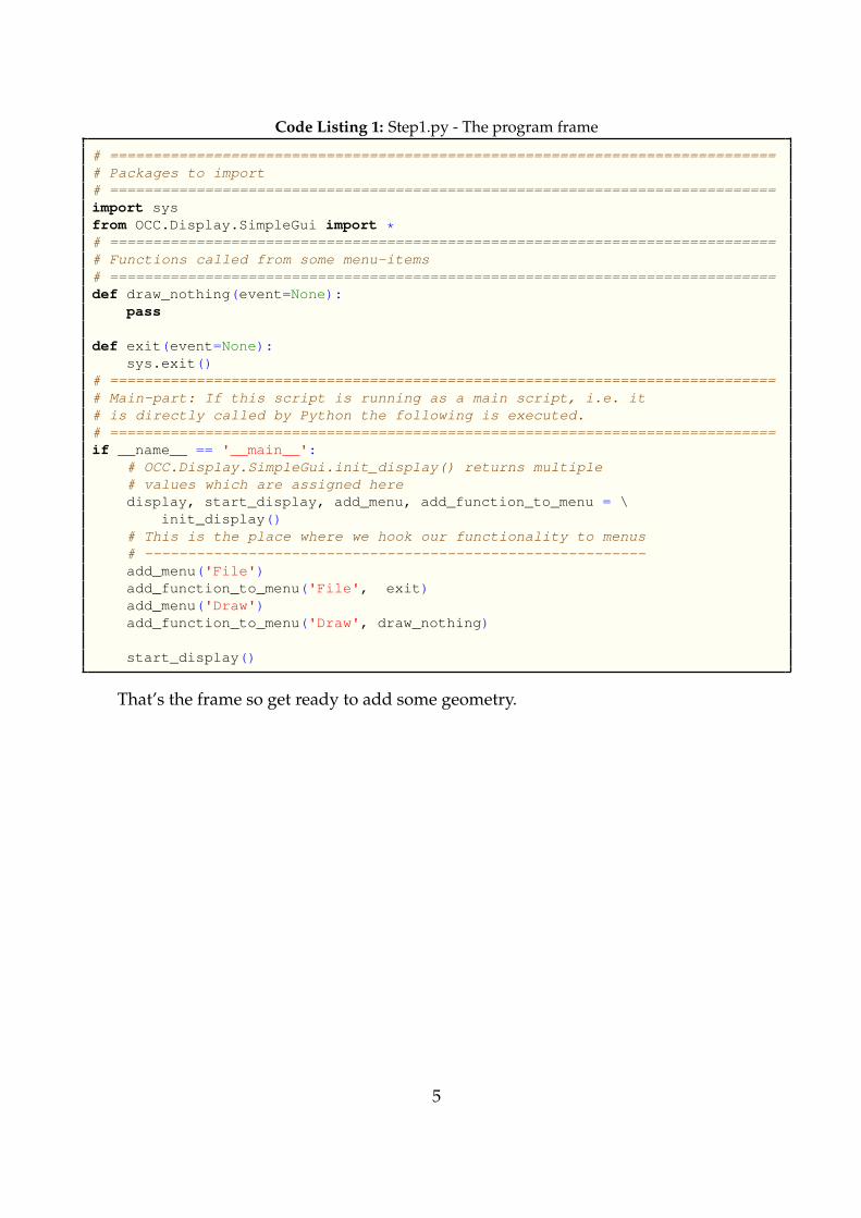
Code Listing 1: Step1.py - The program frame

# =============================================================================# Packages to import# =============================================================================import sysfrom OCC.Display.SimpleGui import *# =============================================================================# Functions called from some menu-items# =============================================================================def draw_nothing(event=None):

pass

def exit(event=None):sys.exit()

# =============================================================================# Main-part: If this script is running as a main script, i.e. it# is directly called by Python the following is executed.# =============================================================================if __name__ == '__main__':

# OCC.Display.SimpleGui.init_display() returns multiple# values which are assigned heredisplay, start_display, add_menu, add_function_to_menu = \

init_display()# This is the place where we hook our functionality to menus# ----------------------------------------------------------add_menu('File')add_function_to_menu('File', exit)add_menu('Draw')add_function_to_menu('Draw', draw_nothing)

start_display()

That’s the frame so get ready to add some geometry.

5

2 Step 2 - Drawing Spheres

2.1 Drawing spheres from points

Our first sample which adds some geometric objects is pretty simple. Execute Step2_1.py,click on menu Drawmenu-item draw sphere 1 and after that click on menu Drawmenu-item draw sphere 2 to see the screen shown in figure 2. If you click on menu Erase

menu-item erase all the whole canvas will be erased.

Figure 2: Screenshot of Step2_1

Time to learn navigating with the mouse! Display both spheres utilising the menu. Dothe following:

1. Move the mouse into the screen, press the left mouse button and hold it down. Movethe mouse with the left mouse button pressed down. See that the coordinate systemin the right corner at the bottom and the objects turn according to your mouse moves.So moving the mouse with the left mouse button held down rotates the model. Thiscannot be seen with one sphere because a sphere looks the same from every side.

2. Press the middle mouse button and move the mouse. This causes a translation of thespheres.

3. Hold down the right mouse button and move the mouse to the left. The objects movesaway from you. Now move the mouse to the right with the right mouse button helddown. The objects come closer.

6

Let’s have a look at the code. Listing 2 shows how the menu and menu-items werechanged to make the new funcionality available in the graphical use interface.

Code Listing 2: Step2_1.py - Extending the menu

...# This is the place where we hook our functionality to menus# ----------------------------------------------------------add_menu('File')add_function_to_menu('File', exit)add_menu('Draw')add_function_to_menu('Draw', draw_sphere_1)add_function_to_menu('Draw', draw_sphere_2)add_menu('Erase')add_function_to_menu('Erase', erase_all)

...

As you can see in listing 3 there are two functions draw_sphere_1 and draw_sphere_2

added under menu Draw. The new menu Erase is bound to function erase_all. Thesefunctions are presented in listing 3. It should also be noted that we have to import twoadditional modules OCC.gp and OCC.BRepPrimAPI.

Code Listing 3: Step2_1.py - Extending the functionality

# =============================================================================# Packages to import# =============================================================================import sysfrom OCC.Display.SimpleGui import *from OCC.gp import *from OCC.BRepPrimAPI import *

# =============================================================================# Functions called from some menu-items# =============================================================================def draw_sphere_1(event=None):

# create sphereRadius = 50.0# The sphere centerX1 = 0.0Y1 = 0.0Z1 = 0.0# create OCC.gp.gp_Pnt-Point from vectorPoint = gp_Pnt( X1, Y1, Z1 )MySphere = BRepPrimAPI_MakeSphere( Point, Radius )MySphereShape = MySphere.Shape()display.DisplayColoredShape( MySphereShape , 'RED' )

def draw_sphere_2(event=None):# create sphereRadius = 50.0# The sphere centerX1 = 25.0

7

Y1 = 50.0Z1 = 50.0# create OCC.gp.gp_Pnt-Point from vectorPoint = gp_Pnt( X1, Y1, Z1 )MySphere = BRepPrimAPI_MakeSphere( Point, Radius )MySphereShape = MySphere.Shape()display.DisplayColoredShape( MySphereShape , 'YELLOW' )

def erase_all(event=None):display.EraseAll()

...

A sphere is a so called primitive. Boxes, tori, wedges, cylinders and cones are other prim-itives which are also availble in pythonOCC. To make use of these primitives we haveto import OCC.BRepPrimAPI. In this course we will generate a lot of primitives so youcan see how it works. It should be noted that there are different constructors availablefor single primitives. Please refer to the pythonOCC [4] documentation to see how theseare constructed. Sometimes consulting the C++ documentation of Open Cascade [5] isalso be helpful. In addition the Modelling Algorithms Users Guide which is available at theOpen Cascade web-site too offers additional information. The latter does not contain everypossibility so I recommend to read the documentation in html.

If we want to create and draw a primitive we always perform three steps.

1. Generate the primitive utilzing a constructor likeMySphere=BRepPrimAPI_MakeSphere(Point,Radius)

2. Create the shape of the primitive5

MySphereShape = MySphere.Shape()

3. Display the shapedisplay.DisplayColoredShape( MySphereShape , ’YELLOW’ )

The constructor used in our code receives a variable Point and a variable Radius.Radius is obviously just a floating point value but Point is something that has to be cre-ated byPoint = gp_Pnt( X1, Y1, Z1 )

where X1, X2 and X3 are floating point values. Module OCC.gp contains definitions ofdifferent geometric objects like points, circles, axes, directions and so on which are ac-cepted by pythonOCC. The natural way to define a sphere is to specify a point at the center

5Until now I did not find out why this has to be done and what exactly is the difference of the primitiveand its shape. But believe me we are able to make use of pythonOCC for our visualization purposes withoutthat knowledge. As soon as I understand the background I will update the document. Thomas Paviot recom-mended to read Roman Lygin’s blog http://opencascade.blogspot.com/2009/02/topology-and-geometry-in-open-cascade.html especially the pages dedicated to the topology data model. Thomas also announcedsome document concerning that topic.

8

and a radius. Because we are talking to pythonOCC we have to enter the point in a waypythonOCC understands and thats in this case done by the specification of a gp_Pnt ob-ject6.

2.2 Drawing spheres from Scipy arrays

At this point it is time for Scipy to enter the scene. Scipy offers you great functionalityfor doing geometrical computations. pythonOCC and Scipy are a great team which caneasily be combined.

So have a look at Step2_2.py and see that we changed the beginning of the code likeshown in listing 4

Code Listing 4: Step2_1.py - Involve Scipy

# =============================================================================# Packages to import# =============================================================================import sysfrom OCC.Display.SimpleGui import *from OCC.gp import *from OCC.BRepPrimAPI import *import scipy# =============================================================================# Functions generating primitives from Scipy arrays# =============================================================================def sphere_from_vector_and_radius( vector,

radius ):'''Creates a sphere from a scipy vector and a radius

@param vector: center of a sphere as a scipy array@type vector: array(3,1)@param radius: radius of the sphere@type radius: scalar'''# write the components of vector in float valuesX1 = float( vector[ 0, 0] )Y1 = float( vector[ 1, 0] )Z1 = float( vector[ 2, 0] )# create OCC.gp.gp_Pnt-Point from vectorPoint = gp_Pnt( X1, Y1, Z1 )# create spheresphere = BRepPrimAPI_MakeSphere( Point, radius )# retrurn the spherereturn sphere

6In pythonOCC objects carry their module names as a prefix. This helps if you have to read samplescontaining functions imported via from some_module import *. Simply look at the prefix and you knowthe home module of the object.

9

# =============================================================================# Functions called from some menu-items# =============================================================================def draw_sphere_1(event=None):

# create sphereRadius = 50.0# The sphere center as a Scipy array - 3 rows, one column# Note we use the scipy.zeros functionPointZeroArray = scipy.zeros((3,1), dtype=float)MySphere = sphere_from_vector_and_radius( PointZeroArray,

Radius )MySphereShape = MySphere.Shape()display.DisplayColoredShape( MySphereShape , 'RED' )

def draw_sphere_2(event=None):# create sphereRadius = 50.0# The sphere center as a Scipy array - 3 rows, one columnMyPointAsArray = scipy.array([25.0, 50.0, 50.0])MyPointAsArray = scipy.reshape(MyPointAsArray,(3,1))MySphere = sphere_from_vector_and_radius( MyPointAsArray,

Radius )MySphereShape = MySphere.Shape()display.DisplayColoredShape( MySphereShape , 'YELLOW' )

...

If you run Step2_2.py you get the same result as you got from Step2_1.py. The dif-ference between these programs lies in the construction of the sphere. In Step2_1.py

we defined three floating point values and generated a gp_Pnt object. In Step2_2.py aScipy array is used for that purpose.

Functions draw_sphere_1 and draw_sphere_2 are creating an array. The first onedoes this by calling scipy.zeros the latter on by scipy.array so you can realize thatboth options work.

Now function sphere_from_vector_and_radius is called. Here we construct thesphere. Experience showed that it is always a good idea to cast the content of the array inthe way shown below.

...# write the components of vector in float valuesX1 = float( vector[ 0, 0] )Y1 = float( vector[ 1, 0] )Z1 = float( vector[ 2, 0] )

...

10

3 Step 3 - Boolean Operations

3.1 What are Boolean Operations?

In the last step we learned how to construct spheres. Spheres are a member some sort ofobjects called primitives. Combining primitives can be used to build more complicatedstructures. Think of combinations like add, subtract and difference. For example you mayask for the volume which is occupied by a sphere without the volume occupied by anothersphere.

If you’ve taken set theory at school you probably drawed so called Venn diagrams.These diagrams work analog to the Boolean operations offered in pythonOCC. Figure 3illustrates the Boolean operations of two overlapping sets A and B utilising Venn diagrams.

(a) Set A (b) Set B (c) Set A or set B (A ∪B)

(d) Set A and set B (A ∩B) (e) Set A without set B (A \B) (f) Set B without set A (B \A)

Figure 3: Sets and their Boolean combinations

If you created two primitives pythonOCC can perform Boolean operations analog tothose sketched in figure 3. Sometimes this is called Constructive Solid Geometry (CSG). Youneed to import OCC.BRepAlgoAPI into your code because this functionality resides inthat module. The main functions are:

1. BRepAlgoAPI_Fuse combines two primitives so that the resulting object occupiesthe space of both source objects. This is equivalent to the or-operation (symbol ∪)shown in figure 3(c).

11

2. BRepAlgoAPI_Common combines two primitives so that the resulting object occu-pies the overlapping space of both source objects. This is equivalent to the and-operation (symbol ∩) shown in figure 3(d).

3. BRepAlgoAPI_Cut combines two primitives so that the resulting object occupies thespace of the first source object minus the space ocuppied by the second source object.This is equivalent to the without-operation (symbol \) shown in figures 3(e) and 3(f).

3.2 A first sample on Boolean operations in pythonOCC

In order to see how things work execute sample Step3_1.py, click on menu Draw menu-item draw sphere 1 and after that click on menu Draw menu-item draw sphere 2.Please note that before drawing the new object the screen is erased. Use the new menuBoolean and select the menu-items. Turn the objects so you can see their shape.

The menu-items should be self explaining so let’s look at the code. Listing 5 showshow the menu and menu-items were changed to make the new funcionality available inthe graphical use interface.

Code Listing 5: Step3_1.py - Extending the menu

...# This is the place where we hook our functionality to menus# ----------------------------------------------------------add_menu('File')add_function_to_menu('File', exit)add_menu('Draw')add_function_to_menu('Draw', draw_sphere_1)add_function_to_menu('Draw', draw_sphere_2)add_menu('Boolean')add_function_to_menu('Boolean', draw_fused_spheres)add_function_to_menu('Boolean', draw_cutted_spheres_1)add_function_to_menu('Boolean', draw_cutted_spheres_2)add_function_to_menu('Boolean', draw_common_spheres)add_menu('Erase')add_function_to_menu('Erase', erase_all)

...

This should not be a suprise if you studied the code of the former steps. So in the next stepwe do not discuss that anymore. If you are unsure look at the code.

Listing 6 shows two of the new functions added under menu Boolean.

Code Listing 6: Step3_1.py - Extending the functionality

def draw_cutted_spheres_2(event=None):# clear the displaydisplay.EraseAll()# create sphere

12

Radius = 50.0# The sphere center as a Scipy array - 3 rows, one column# Note we use the scipy.zeros functionPointZeroArray = scipy.zeros((3,1), dtype=float)MySphere1 = sphere_from_vector_and_radius( PointZeroArray,

Radius )MySphere1Shape = MySphere1.Shape()

# The sphere center as a Scipy array - 3 rows, one columnMyPointAsArray = scipy.array([25.0, 50.0, 50.0])MyPointAsArray = scipy.reshape(MyPointAsArray,(3,1))MySphere2 = sphere_from_vector_and_radius( MyPointAsArray,

Radius )MySphere2Shape = MySphere2.Shape()# Combine the spheresCuttedSpheres = OCC.BRepAlgoAPI.BRepAlgoAPI_Cut( MySphere2Shape,

MySphere1Shape )# Shape of combined spheresCuttedSpheres = CuttedSpheres.Shape()# Displaydisplay.DisplayColoredShape( CuttedSpheres , 'BLUE' )

def draw_common_spheres(event=None):# clear the displaydisplay.EraseAll()# create sphereRadius = 50.0# The sphere center as a Scipy array - 3 rows, one column# Note we use the scipy.zeros functionPointZeroArray = scipy.zeros((3,1), dtype=float)MySphere1 = sphere_from_vector_and_radius( PointZeroArray,

Radius )MySphere1Shape = MySphere1.Shape()

# The sphere center as a Scipy array - 3 rows, one columnMyPointAsArray = scipy.array([25.0, 50.0, 50.0])MyPointAsArray = scipy.reshape(MyPointAsArray,(3,1))MySphere2 = sphere_from_vector_and_radius( MyPointAsArray,

Radius )MySphere2Shape = MySphere2.Shape()# Combine the spheresCommonSpheres = OCC.BRepAlgoAPI.BRepAlgoAPI_Common( MySphere1Shape,

MySphere2Shape )# Shape of combined spheresCommonSpheres = CommonSpheres.Shape()# Displaydisplay.DisplayColoredShape( CommonSpheres , 'GREEN' )

...

At the beginning of these functions the canvas is erased. After that two sphere shapes arecreated in exactly the same manner as in listing 4. The next lines provide something new.As the comment tells the spheres are combined.

Function draw_cutted_spheres_2 performs the Boolean without operation utilising

13

the function BRepAlgoAPI_Cut. The function takes two shapes of primitives and deliversthe result first primitive without second primitive. If you change the order of the argumentsgiven to function BRepAlgoAPI_Cut the Boolean operation is also changed like shown infunction draw_cutted_spheres_1.

Next we look at function draw_common_spheres. Note that the function is similarto function draw_cutted_spheres_2. The Boolean operation is the main difference be-tween these functions. In draw_common_spheres function BRepAlgoAPI_Common isused to perform the and operation.

Please note the similarity of both Boolean operations discussed. Combing two primi-tives is always done in the same manner.

1. Construct Primitive_1

2. Create the shape Shape_1 = Primitive_1.Shape()

3. Construct Primitive_2

4. Create the shape Shape_2 = Primitive_2.Shape()

5. Perform the Boolean operation between Shape_1 and Shape_2 to get a New_Object

6. Create New_Object.Shape() before displaying it

3.3 Extending the first sample on Boolean operations in pythonOCC

3.3.1 What we want to do and how it looks like

Now that we know how to construct and combine primitives we should practice our newabilities. What about drawing other things like a cylinder, a cone and an arrow? Oh no,unfortunately there is no primitive creating arrows available. So forget about the last one.Stop! We learned how to use Boolean operations so lets use a cone and a cylinder for thearrow and combine these.

Execute Step3_2.py to see how we extend our sample. Please use menu Draw andtry the new functions draw cylinder, draw cone and draw arrow. Also note that incontrast to Step3_1.py the functions under menu Draw do not erase the canvas. Henceall objects remain there until you use function erase all or until you use one of the itemsunder menu Boolean or until you close the program. Figure 4 shows how the canvas canlook if you choose all objects from menu Draw. If you do the same you will see the objectsbut the perspective may differ.

14

Figure 4: Screenshot of Step3_2

3.3.2 Creating a cylinder

We start with the creation of the cylinder object7. Listing 78 presents the complete function.Skim over it so we can go into the details in the following paragraphs.

Code Listing 7: Step3_2.py - Defining a cylinder from a point, a direction vector, the length andthe radius

def cylinder_from_point_directionvector_length_and_radius( vector,directionvector,length,radius ):

"""Creates a cylinder utilising OCC.BRepPrimAPI.BRepPrimAPI_MakeCylinder outof scipy arrays

@param vector: vektor of starting point on the cylinder main axis

7Maybe you ask yourself: Should I start learning how to use the OpenCascade documentation and practisebeside working on that introduction? If you want that open the C++ documentation of Open Cascade [5] andread the constructors for a cylinder. You don’t need to do that now but you definitely have to do that if youcreate own applications. So start using it whenever you think you are ready for it and learn how to go aroundin the docu. No fear! If you honor the structure shown in the C++ documentation and think in Python codeyou will learn using the application of the C++ documentation to create your own code although it is Pythonand not C++. If you want to keep focused on what is presented here that’s also ok. The intention of that hintis only to encourage the reader to use the documentation. To some extent the way of learning is different forevery individual so you need to decide how to learn.

8Please note the marvellous documentation strings. This is epytext a very easy markaup language forEpydoc [1] a very efficient documentation tool. In my opinion it is worth a trial.

15

@type vector: scipy array(3,1)@param directionvector: direction vector of the cylinder main axis@type directionvector: scipy array(3,1)@param length: cylinder length@type length: float@param radius: cylinder radius@type radius: float@return: cylinder

sample::

Vector = scipy.array([ 10.0, 10.0, 10.0 ])Vector = scipy.reshape( Vector, (3,1))

TangUnitVector = scipy.array([ (1/scipy.sqrt(3)) ,1/scipy.sqrt(3)) ,1/scipy.sqrt(3)) ])

TangUnitVector = scipy.reshape( TangUnitVector, (3,1))

CylLength = 200CylRadius = 3

Cyli = cylinder_from_point_directionvector_length_and_radius(Vector,TangUnitVector,CylLength,CylRadius )

CyliShape = Cyli.Shape()display.DisplayColoredShape( CyliShape , 'RED' )

"""# Normalize the directiondirectionunitvector = NormVector(directionvector)# determine the second pointvector2 = vector + length * directionunitvector# components of vector in float valuesX1 = float( vector[ 0, 0] )Y1 = float( vector[ 1, 0] )Z1 = float( vector[ 2, 0] )# components of vector2 in float valuesX2 = float( vector2[ 0, 0] )Y2 = float( vector2[ 1, 0] )Z2 = float( vector2[ 2, 0] )# create OCC.gp.gp_Pnt-pointsP1 = OCC.gp.gp_Pnt( X1, Y1, Z1 )P2 = OCC.gp.gp_Pnt( X2, Y2, Z2 )# create direction unit vector from these points (not neccessary but if# the directionunitvector is not of length 1 ...)directionP1P2 = scipy.array([ ( X2 - X1 ),

( Y2 - Y1 ),( Z2 - Z1 ) ])

directionP1P2 = scipy.reshape( directionP1P2,(3,1))# distance between the points (X1, Y1, Z1) and (X2, Y2, Z2)length = length_column_vector(directionP1P2)# normalize directiondirectionP1P2 = NormVector(directionP1P2)

16

# origin at point 1 with OCC.gp.gp_Pntorigin_local_coordinate_system = OCC.gp.gp_Pnt( X1, Y1, Z1)# z-direction of the local coordinate system with OCC.gp.gp_Dirz_direction_local_coordinate_system = OCC.gp.gp_Dir(directionP1P2[0, 0],

directionP1P2[1, 0],directionP1P2[2, 0])

# local coordinate system with OCC.gp.gp_Ax2local_coordinate_system = OCC.gp.gp_Ax2(origin_local_coordinate_system,

z_direction_local_coordinate_system)# create cylinder utilising OCC.BRepPrimAPI.BRepPrimAPI_MakeCylindercylinder = OCC.BRepPrimAPI.BRepPrimAPI_MakeCylinder(local_coordinate_system,

radius,length,2 * scipy.pi )

# return cylinderreturn cylinder

Function cylinder_from_point_directionvector_length_and_radius is heav-ily commented so studying the code should be possible. Anyhow a few words may help.As the function name implies we construct the cylinder from a point, a direction vector, thelength and the radius. The first two parameters have to be Scipy arrays the other two arefloating point values.

We start with the normalization of the direction vector.

# Normalize the directiondirectionunitvector = NormVector(directionvector)

We utilize function NormVector which uses function length_column_vector. Bothfunctions are found in the source. The first takes a direction vector of arbitrary length andreturns a direction vector of length one with the same direction, the latter one determinesthe length of a vector.We get one center point at one end of the cylinder from the parameters. So we compute thecenter point at the other end.

# determine the second pointvector2 = vector + length * directionunitvector

As already mentioned casting the contents of a Scipy array to floats avoided some myste-rious error messages. Note that we do not mention that in the next sections. Please have alook at the following lines and try to keep them in mind.

# components of vector in float valuesX1 = float( vector[ 0, 0] )Y1 = float( vector[ 1, 0] )Z1 = float( vector[ 2, 0] )

The construction of points OCC.gp.gp_Pnt was already shown

17

# create OCC.gp.gp_Pnt-pointsP1 = OCC.gp.gp_Pnt( X1, Y1, Z1 )

but here is something new.

# z-direction of the local coordinate system with OCC.gp.gp_Dirz_direction_local_coordinate_system = OCC.gp.gp_Dir(directionP1P2[0, 0],

directionP1P2[1, 0],directionP1P2[2, 0])

Thats the direction of the cylinder in pythonOCC termonology. It serves as a local z-coordinate for our cylinder primitive. The constructor used a few lines later constructsa cylinder accoding to a local coordinate system. The main axis of the cylinder created isthe z-coordinate of that local coordinate system. So it is no suprise that with

# local coordinate system with OCC.gp.gp_Ax2local_coordinate_system = OCC.gp.gp_Ax2(origin_local_coordinate_system,

z_direction_local_coordinate_system)

a local coordinate is introduced. What about the x- and y-direction of the local coordinatesystem? The answer is: I don’t know. But remember the cylinder is oriented along thez-axis and we do not care about x and y. The cross section of the cylinder is a circle so whocares about that?Now we are ready to create and return the cylinder object.

# create cylinder utilising OCC.BRepPrimAPI.BRepPrimAPI_MakeCylindercylinder = OCC.BRepPrimAPI.BRepPrimAPI_MakeCylinder(local_coordinate_system,

radius,length,2 * scipy.pi )

# return cylinderreturn cylinder

We are in possession of a function creating cylinder objects. Please read listing 8 to seehow we call it from function draw_cylinder.

Code Listing 8: Step3_2.py - Calling the function defining a cylinder from a point, a directionvector, the length and the radius

def draw_cylinder(event=None):# cylinder radiusRadius = 50.0# cylinder lengthLength = 200.0# The center point at one of the flat cylinder facesPoint = scipy.array([45.0, 80.0, 50.0])Point = scipy.reshape(Point,(3,1))# The direction of the cylinder from the point given aboveDirectionFromPoint = scipy.array([25.0, 50.0, 150.0])

18

DirectionFromPoint = scipy.reshape(DirectionFromPoint,(3,1))# create the cylinder objectMyCylinder = cylinder_from_point_directionvector_length_and_radius( \

Point,DirectionFromPoint,Length,Radius )

MyCylinderShape = MyCylinder.Shape()display.DisplayColoredShape( MyCylinderShape , 'BLUE' )

Do you recognize the similarity of that function to the functions used to call the functioncreating spheres? It works exactly like those.

3.3.3 Creating a cone

If you followed the explainations of section 3.3.2 you will easily get the cone too. Havea look at code listing 9. It shows the whole function. Please read it and think about thesimilarity betwen listing 8 and 9. Note that a cone is a cylinder exhibiting two differentradi at the end so we need two radi to construct it.

Code Listing 9: Step3_2.py - Function defining a cone from a point, a direction vector, theheight and two radi

def cone_from_point_height_directionvector_and_two_radii( vector,directionvector,height,radius1,radius2 ):

"""Creates a cone OCC.BRepPrimAPI.BRepPrimAPI_MakeCone.

@param vector: vector at the beginning@type vector: scipy array(3,1)@param directionvector: direction vector of the cone maina axis@type directionvector: scipy array(3,1)@param height: cone height@type height: float@param radius1: radius at the cone bottom@type radius1: float@param radius1: cone tip radius@type radius1: float@return: cone"""# Normalize the directiondirectionunitvector = NormVector(directionvector)# Determine the second pointvector2 = vector + height * directionunitvector# components in floatsX1 = float( vector[ 0, 0] )Y1 = float( vector[ 1, 0] )Z1 = float( vector[ 2, 0] )

19

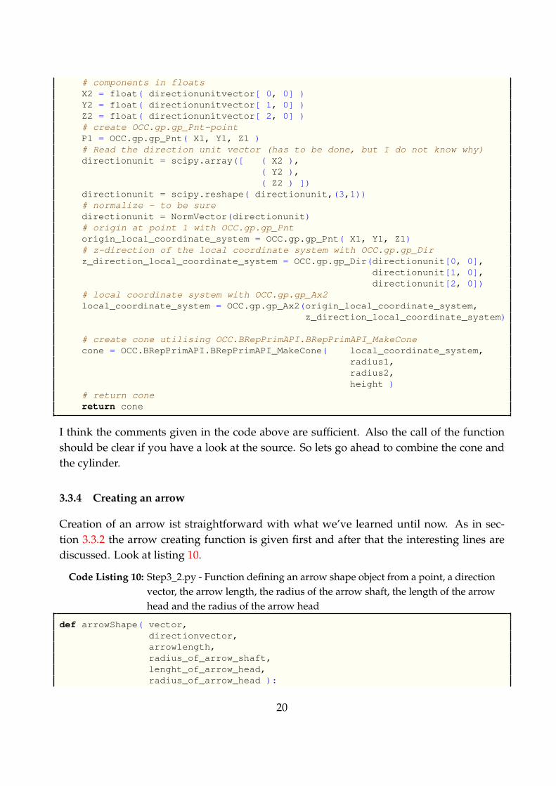
# components in floatsX2 = float( directionunitvector[ 0, 0] )Y2 = float( directionunitvector[ 1, 0] )Z2 = float( directionunitvector[ 2, 0] )# create OCC.gp.gp_Pnt-pointP1 = OCC.gp.gp_Pnt( X1, Y1, Z1 )# Read the direction unit vector (has to be done, but I do not know why)directionunit = scipy.array([ ( X2 ),

( Y2 ),( Z2 ) ])

directionunit = scipy.reshape( directionunit,(3,1))# normalize - to be suredirectionunit = NormVector(directionunit)# origin at point 1 with OCC.gp.gp_Pntorigin_local_coordinate_system = OCC.gp.gp_Pnt( X1, Y1, Z1)# z-direction of the local coordinate system with OCC.gp.gp_Dirz_direction_local_coordinate_system = OCC.gp.gp_Dir(directionunit[0, 0],

directionunit[1, 0],directionunit[2, 0])

# local coordinate system with OCC.gp.gp_Ax2local_coordinate_system = OCC.gp.gp_Ax2(origin_local_coordinate_system,

z_direction_local_coordinate_system)

# create cone utilising OCC.BRepPrimAPI.BRepPrimAPI_MakeConecone = OCC.BRepPrimAPI.BRepPrimAPI_MakeCone( local_coordinate_system,

radius1,radius2,height )

# return conereturn cone

I think the comments given in the code above are sufficient. Also the call of the functionshould be clear if you have a look at the source. So lets go ahead to combine the cone andthe cylinder.

3.3.4 Creating an arrow

Creation of an arrow ist straightforward with what we’ve learned until now. As in sec-tion 3.3.2 the arrow creating function is given first and after that the interesting lines arediscussed. Look at listing 10.

Code Listing 10: Step3_2.py - Function defining an arrow shape object from a point, a directionvector, the arrow length, the radius of the arrow shaft, the length of the arrowhead and the radius of the arrow head

def arrowShape( vector,directionvector,arrowlength,radius_of_arrow_shaft,lenght_of_arrow_head,radius_of_arrow_head ):

20

'''Function arrowshape creates the shape of an arrow starting at vectorpointing into diretcion. We create a cylinder and a cone and combine theutilising OCC.BRepAlgoAPI.BRepAlgoAPI_Fuse.

@param vector: starting point of the arrow@type vector: scipy array(3,1)@param directionvector: direction of the arrow@type directionvector: scipy array(3,1)@param arrowlength: length of the arrow@type arrowlength: scalar@param radius_of_arrow_shaft: radius of the arrow shaft@type radius_of_arrow_shaft: scalar@param lenght_of_arrow_head: length of the arrow head@type lenght_of_arrow_head: scalar@param radius_of_arrow_head: radius of the arrow head@type radius_of_arrow_head: scalar@return: Pfeil als Shape Objekt'''# Normalize the directiondirectionunitvector = NormVector(directionvector)# the shaft lengthcylinder_length = arrowlength - lenght_of_arrow_head# create shaftarrow_shaft = cylinder_from_point_directionvector_length_and_radius( \

vector,directionunitvector,cylinder_length,radius_of_arrow_shaft )

arrow_shaft_Shape = arrow_shaft.Shape()# begin of arrow head (flat suface)arrow_head_point = vector + cylinder_length * directionunitvector# create arrow headarrow_head = cone_from_point_height_directionvector_and_two_radii( \

arrow_head_point,directionunitvector,lenght_of_arrow_head,radius_of_arrow_head,0.0 )

arrow_head_Shape = arrow_head.Shape()# combine shaft and headarrow = OCC.BRepAlgoAPI.BRepAlgoAPI_Fuse( arrow_shaft_Shape,

arrow_head_Shape )arrowShape = arrow.Shape()# return Shape of the arrowreturn arrowShape

Did you recognize the different return type here? In code listing 8 and 9 we returned thegeometric object here we return the shape of the object. Why do we do that? Only todemonstrate that it is also possible to return the shape of the object.

We start our examination with a look at figure 4. Our arrow consists of a cylindricalshaft and a conic head. The heads cone has two radi. One of it is zero. That’s the tip of the

21

arrow. The other one is larger than the radius of the cylindrical shaft.

The first lines of code listing 10 build the cylinder shape of the shaft. To get the length ofthe shaft we subtract the length of the head from the total length of the arrow. Both valuesare given in the parameter set.

# Normalize the directiondirectionunitvector = NormVector(directionvector)# the shaft lengthcylinder_length = arrowlength - lenght_of_arrow_head# create shaftarrow_shaft = cylinder_from_point_directionvector_length_and_radius( \

vector,directionunitvector,cylinder_length,radius_of_arrow_shaft )

arrow_shaft_Shape = arrow_shaft.Shape()

Next the shape of the conic head is constructed. We need to compute the beginning of thecone so we walk the length of the shaft from the starting point of the arrow into the arrowsdirection to reach the flat side of the conic arrow head. Here we create the cone which hasone radius of zero. I simply tried which radius is the right one. That’s the way things canbe solved if you are to lazy for studying the documentation.

# begin of arrow head (flat suface)arrow_head_point = vector + cylinder_length * directionunitvector# create arrow headarrow_head = cone_from_point_height_directionvector_and_two_radii( \

arrow_head_point,directionunitvector,lenght_of_arrow_head,radius_of_arrow_head,0.0 )

arrow_head_Shape = arrow_head.Shape()

Both shapes, the cylinder shape and the cone shape, are then glued together to form thearrow object. See how easy it is to construct new objects with the aid of Boolean operations.

# combine shaft and headarrow = OCC.BRepAlgoAPI.BRepAlgoAPI_Fuse( arrow_shaft_Shape,

arrow_head_Shape )

As already mentioned in that function we do not return the object we return its shape.Whether there are advatages or disadvantages between returning the shape or the object Icannot tell. But as you can see both options deliver the same result.

arrowShape = arrow.Shape()# return Shape of the arrowreturn arrowShape

22

Note if you return the shape to a calling function this calling function must not call theShape() method again. If it does that a error will happen.

If you cannot imagine how the function is called and how the shape is drawn pleaselook at the code. Function draw_arrow which is hooked into the menu does the job inexactly the same manner as the one building the spheres, the cylinder and the cone. Thesefunctions define the needed parameters, call the appropriate function to create the objectand display the shape of the created object.

This was much more a jump then a step. If you got that so far you are at least preparedfor discussions dealing with Constructive solid geometry (CSG) and Boolean operations. That’snot so bad!

23

4 Step 4 - Time for Practice

4.1 Extending our sample

The last sample of the former section is now used as a starting point for getting somepractice.

Did you notice the little coordinate cross at the bottom of the screen? It shows youthe x-, y- and z-direction in the displayed space. To get some practice we place a largercoordinate cross at the origin. Execute Step4_1.py, click on menu Draw menu-item draw

coordinates to get the screen shown in figure 5.

Figure 5: Screenshot of Step4_1

To see how this is done start reading Listing 11 where the function which is called afterselecting that menu item is presented. The function is heavily commented and should beunderstood without difficulty.

Code Listing 11: Step4_1.py - Drawing a larger, coloured coordinate system – functiondraw_coordinates which is called by clicking on the menu

def draw_coordinates(event=None):# The radius of a sphere at the origincenterpoint_sphere_radius = 30.0# The length of every axis starting at -length/2 and ending at length/2arrowlength = 1000.0# Radius of the arrow shaft of every axisradius_of_arrow_shaft = 10.0

24

# Length of every axislenght_of_arrow_head = 50.0# Radius of the arrow heads coneradius_of_arrow_head = 20.0# Create the Coordinate and Draw itCoordinateCrossShape( centerpoint_sphere_radius,

arrowlength,radius_of_arrow_shaft,lenght_of_arrow_head,radius_of_arrow_head )

Function draw_coordinates calls CoordinateCrossShape. We should also havea look at that function given in Listing 12. Before you start reading the code let me statethat all the functionality used in that function was already explained in the last section. Ialso like to mention that the different parts of the coordinate cross are not combined byBoolean functions. On one hand this makes it easy to apply different colours to the singleparts on the other there is no need to move or turn the coordinate axis - these are our worldcoordinates. Finally I would like to guide your attention at the end of the function. It doesnot return anything. The function itself draws the coordinate cross.

Code Listing 12: Step4_1.py - Drawing a coordinate system – functionCoordinateCrossShape which is called by function draw_coordinates

def CoordinateCrossShape( centerpoint_sphere_radius,arrowlength,radius_of_arrow_shaft,lenght_of_arrow_head,radius_of_arrow_head ):

'''Function arrowshape creates the shape of an arrow starting at vectorpointing into diretcion. We create a cylinder and a cone and combine theutilising OCC.BRepAlgoAPI.BRepAlgoAPI_Fuse.

@param vector: starting point of the arrow@type vector: scipy array(3,1)@param directionvector: direction of the arrow@type directionvector: scipy array(3,1)@param arrowlength: length of the arrow@type arrowlength: scalar@param radius_of_arrow_shaft: radius of the arrow shaft@type radius_of_arrow_shaft: scalar@param lenght_of_arrow_head: length of the arrow head@type lenght_of_arrow_head: scalar@param radius_of_arrow_head: radius of the arrow head@type radius_of_arrow_head: scalar@return: Arrow as Shape object'''# The origin of the coordinate systemOrigin = scipy.zeros((3,1),dtype=float)# The direction unit vectors of the axisxDir = scipy.zeros((3,1),dtype=float)

25

xDir[0,0] = 1.0yDir = scipy.zeros((3,1),dtype=float)yDir[1,0] = 1.0zDir = scipy.zeros((3,1),dtype=float)zDir[2,0] = 1.0

# Create the center point sphere shape at the originOriginSphere = sphere_from_vector_and_radius( Origin,

centerpoint_sphere_radius )OriginSphereShape = OriginSphere.Shape()

# Create the XAxis shapeXAxisShape = arrowShape( Origin - 0.5 * arrowlength * xDir,

xDir,arrowlength,radius_of_arrow_shaft,lenght_of_arrow_head,radius_of_arrow_head )

# Create the YAxis shapeYAxisShape = arrowShape( Origin - 0.5 * arrowlength * yDir,

yDir,arrowlength,radius_of_arrow_shaft,lenght_of_arrow_head,radius_of_arrow_head )

# Create the ZAxis shapeZAxisShape = arrowShape( Origin - 0.5 * arrowlength * zDir,

zDir,arrowlength,radius_of_arrow_shaft,lenght_of_arrow_head,radius_of_arrow_head )

# Display these shapesdisplay.DisplayColoredShape( OriginSphereShape , 'WHITE' )display.DisplayColoredShape( XAxisShape , 'BLUE' )display.DisplayColoredShape( YAxisShape , 'ORANGE' )display.DisplayColoredShape( ZAxisShape , 'GREEN' )

Why is it possible to draw on the display without receiving it as a parameter? Thereason is that the display is created outside of a class or function. Look at the end ofStep4_1.py which is shown in Listing 13.

Code Listing 13: Step4_1.py - Creating the display

if __name__ == '__main__':# OCC.Display.SimpleGuiinit_display() returns multiple# values which are assigned heredisplay, start_display, add_menu, add_function_to_menu = \

OCC.Display.SimpleGui.init_display()...

start_display()

26

4.2 Time for Housekeeping

Our sample became pretty large. So lets divide it into two parts:

Step4_2.py the main program and

Step4_2_A.py a module containing the Scipy stuff and the construction of geometricobjects.

Run program Step4_2.py and see that it works exactly like Step4_1.py. Sure you knowhow this division works. We simply took some functions from Step4_1.py and put theseinto a module called Step4_2_A.py. The remaining main script is called Step4_2.py.In order to tell Python where to look for the outsourced functions we add

...from Step4_2_A import *...

at the beginning of Step4_2.py. Now have a closer look at Step4_2_A.py. See thatwe also modified function CoordinateCrossShape. Look at the function definition weadded one parameter. It is the parameter display.

def CoordinateCrossShape( display,centerpoint_sphere_radius,arrowlength,radius_of_arrow_shaft,lenght_of_arrow_head,radius_of_arrow_head ):

...

You should also notice that the function call which is done from Step4_2.py uses thatadditional parameter too. Of course, we need a structure of parameters which reflects theparameter line of the function called.

...# Create the Coordinate and Draw itCoordinateCrossShape( display,

centerpoint_sphere_radius,arrowlength,radius_of_arrow_shaft,lenght_of_arrow_head,radius_of_arrow_head )

...

Why do we have to do that? Think about a painter painting for some client. If the clientand the painter are in the same room they can point on the canvas to be painted easily. Ifthese two, the painter and the client, are talking via a phone line and the painter is not inthe clients room containing the canvas the client needs to specify his canvas so the painter

27

knows on where to go and paint on. Note that the painter probably has different clients allof them have their own canvas in their room and all of them may ask the painter to comearound and paint on their canvas. The same is true here.

4.3 Once more: Extending the sample

In this section only a few thing to learn were introduced so far. Hence we should have abrief look at something not mentioned until now.

We already saw that we can write code like

...display.DisplayColoredShape( MyCylinderShape , 'YELLOW' )

...

to draw coloured objects. What if we like to change other things like material and trans-parency? Here the coding gets a little more complicated because we need to be familiarwith the Application Interactive Services (AIS). These services are responsible for the presen-tation including display properties of geometrical structures, display quality, detection andselection.

At the moment I cannot tell how all this can be done and I need to explore the ApplicationInteractive Services (AIS) to see how to make use of them. Nevertheless I want to tell youmy actual knowledge which may help you to get things done if you try to make objectstransparent and so on.

Execute Step4_3.py and choose menu Draw, menu item draw cylinder. Probablyyou cannot see the cylinder without moving away from the scene with the mouse. As analternative choose menu Draw, menu item draw coordinates so all objects are shown.The same is true if you select menu Draw, menu item draw cone. I cannot tell how this canbe avoided but I will add the solution in some future revision of this document if I’ll findany. Select also menu Draw, menu item draw sphere 2. See that the cylinder intersectswith sphere 2. The cylinder is transparent and sphere 2 can be seen through the cylinder.In addition the material of the cone is modified compared to the display in Step4_2.py.Figure 6 shows the screen presented after you reproduced the steps above.

Listing 14 shows the modifications starting at the beginning of Step4_3.py and both,the modified cone and the modified cylinder display. As already mentioned this sample isnot fully understood by me so I only can show how I got it to work.

Code Listing 14: Step4_1.py - Creating the display

...from OCC.AIS import *from OCC.Quantity import *from OCC.Graphic3d import *

28

Figure 6: Screenshot of Step4_3

...def draw_cylinder(event=None):

# cylinder radiusRadius = 50.0# cylinder lengthLength = 200.0# The center point at one of the flat cylinder facesPoint = scipy.array([45.0, 80.0, 50.0])Point = scipy.reshape(Point,(3,1))# The direction of the cylinder from the point given aboveDirectionFromPoint = scipy.array([25.0, 50.0, 150.0])DirectionFromPoint = scipy.reshape(DirectionFromPoint,(3,1))# create the cylinder objectMyCylinder = cylinder_from_point_directionvector_length_and_radius( \

Point,DirectionFromPoint,

Length,Radius )

MyCylinderShape = MyCylinder.Shape()

ais_shape_MyCylinderShape = AIS_Shape( MyCylinderShape ).GetHandle()ais_context = display.GetContext().GetObject()ais_context.SetColor( ais_shape_MyCylinderShape, Quantity_NOC_TOMATO )ais_context.SetTransparency( ais_shape_MyCylinderShape, 0.3, True)ais_context.Display( ais_shape_MyCylinderShape )

def draw_cone(event=None):# cone radius 1Radius1 = 30.0

29

# cone radius 2Radius2 = 70.0# cone heightHeight = 90.0# The center point at one of the flat cone facesPoint = scipy.array([-25.0, -50.0, 50.0])Point = scipy.reshape(Point,(3,1))# The direction of the cone from the point given aboveDirectionFromPoint = scipy.array([25.0, 50.0, 150.0])DirectionFromPoint = scipy.reshape(DirectionFromPoint,(3,1))# create the cone objectMyCone = cone_from_point_height_directionvector_and_two_radii( \

Point,DirectionFromPoint,Height,Radius1,Radius2 )

MyConeShape = MyCone.Shape()ais_shape_MyConeShape = AIS_Shape( MyConeShape ).GetHandle()ais_context = display.GetContext().GetObject()ais_context.SetMaterial( ais_shape_MyConeShape,

Graphic3d.Graphic3d_NOM_STONE )ais_context.Display( ais_shape_MyConeShape )

30

References

[1] Epydoc – Automatic API Documentation Generation for Python.http://epydoc.sourceforge.net/

[2] Python. http://www.python.org/

[3] pythonOCC. http://www.pythonocc.org/

[4] pythonOCC API reference documentation. http://api.pythonocc.org

[5] Open CASCADE. http://www.opencascade.org/

[6] RAPPIN, N.; DUNN, R.: wxPython In Action. Manning Publications Co., GreenwhichCT, USA, 2006

[7] SciPy. http://www.scipy.org/

[8] wxPython. http://www.wxpython.org/

31

A Advanced GUI programming utilizing wx.PySimpleApp

In section 1 the construction of a frame utilizing the OCC.Display.SimpleGuiwas given.You may use the wxPython GUI framework itself. This is shown in listing 15. It producesthe same screen as the one shown in figure 1. To gain a deeper understanding I recommendthe book of Noel Rappin and Robin Dunn [6].

Code Listing 15: Step1.py - The program frame

# =============================================================================# Packages to import# =============================================================================import wximport sys

from OCC import VERSIONfrom OCC.Display.wxDisplay import wxViewer3d

# =============================================================================# Functions called from some menu-items# =============================================================================def draw_nothing(event=None):

pass

def exit(event=None):sys.exit()

# =============================================================================# This is the Application Frame class for wx# =============================================================================class AppFrame(wx.Frame):

def __init__(self, parent):wx.Frame.__init__(self,

parent,-1,

"pythonOCC-%s 3d viewer"%VERSION,style=wx.DEFAULT_FRAME_STYLE,size = (640,480))

self.canva = wxViewer3d(self)self.menuBar = wx.MenuBar()self._menus = {}self._menu_methods = {}

# Function for creating new menus like File, Edit, View, and so on# The stuff appearing at the topdef add_menu(self, menu_name):

_menu = wx.Menu()self.menuBar.Append(_menu, "&"+menu_name)self.SetMenuBar(self.menuBar)self._menus[menu_name]=_menu

# Function for creating new menu items like File-New, File-Exit, Edit-Copy,# Edit-Cut, Edit-paste, and so on

32

# The stuff appearing if a menu is selecteddef add_function_to_menu(self, menu_name, _callable):

_id = wx.NewId()assert callable(_callable), 'the function supplied isnt callable'try:

self._menus[menu_name].Append( \_id,_callable.__name__.replace('_', ' ').lower() )

except KeyError:raise ValueError, 'the menu item %s doesnt exist' % (menu_name)

self.Bind(wx.EVT_MENU, _callable, id=_id)

# =============================================================================# Called from Main-part. Calls itself frame methods.# =============================================================================def add_menu(*args, **kwargs):

frame.add_menu(*args, **kwargs)

def add_function_to_menu(*args, **kwargs):frame.add_function_to_menu(*args, **kwargs)

def start_display():'''call the mainloop'''global appapp.MainLoop()

# =============================================================================# Main-part: If this script is running as a main script, i.e. it# is directly called by Python the following is executed.# =============================================================================if __name__ == '__main__':

# Create Application - with wx.PySimpleApp() we do not need an OnInitapp = wx.PySimpleApp()wx.InitAllImageHandlers()# Create Application Frameframe = AppFrame(None)frame.Show(True)wx.SafeYield()frame.canva.InitDriver()app.SetTopWindow(frame)display = frame.canva._display# Show a background imagedisplay.SetBackgroundImage("bg.bmp")# This is the place where we hook our functionality to menus# ----------------------------------------------------------add_menu('File')add_function_to_menu('File', exit)add_menu('Draw')add_function_to_menu('Draw', draw_nothing)

start_display()

33

B History of this document

0.1 : first public release

34