geometry of special relativity - dray
DESCRIPTION
Great Physics TextbookTRANSCRIPT

THE GEOMETRY OF
SPECIAL RELATIVITY
Tevian DrayDepartment of Mathematics, Oregon State University
8 July 2003

Lorentz transformations are just hyperbolic rotations.
Copyright c© 2000–2003 by Tevian Dray

Preface
The unification of space and time introduced by Einstein’s special theoryof relativity is one of the cornerstones of the modern scientific descriptionof the universe. Yet the unification is counterintuitive, since we perceivetime very differently from space. And, even in relativity, time is not justanother dimension, it is one with different properties. Some authors havetried to “unify” the treatment of time and space, typically by replacing t byit, thus hiding some annoying minus signs. But these signs carry importantinformation: Our universe, as described by relativity, is not Euclidean.
This short book treats the geometry of hyperbolas as the key to under-standing special relativity. This approach can be summarized succinctly asthe replacement of the ubiquitous γ symbol of most standard treatmentswith the appropriate hyperbolic trigonometric functions. In most cases, thisnot only simplifies the appearance of the formulas, but emphasizes their geo-metric content in such a way as to make them almost obvious. Furthermore,many important relations, including but not limited to the famous relativisticaddition formula for velocities, follow directly from the appropriate trigono-metric addition formulas.
I am unaware of any other introductory book on special relativity whichadopts this approach as fundamental. Many books point out the relationshipbetween Lorentz transformations and hyperbolic rotations, but few actuallymake use of it. A pleasant exception was the original edition of Taylor andWheeler’s marvelous book [1], but much of this material was removed fromthe second edition [2].
At the same time, this book is not intended as a replacement for thator any of the other excellent textbooks on special relativity. Rather, it isintended as an introduction to a particularly beautiful way of looking atspecial relativity, in hopes of encouraging students to see beyond the formulasto the deeper structure. Enough applications are included to get the basic
iii
iv PREFACE
idea, but these would probably need to be supplemented for a full course.While much of the material presented can be understood by those fa-
miliar with the ordinary trigonometric functions, occasional use is made ofelementary differential calculus. In addition, the chapter on electricity andmagnetism assumes the reader has seen Maxwell’s equations, and has at leasta passing acquaintance with vector calculus. A prior course in calculus-basedphysics, up to and including electricity and magnetism, should provide thenecessary background.
After a general introduction in Chapter 1, the basic physics of specialrelativity is described in Chapter 2. This is a quick, intuitive introductionto special relativity, which sets the stage for the geometric treatment whichfollows. Chapter 3 summarizes some standard (and some not so standard)properties of ordinary 2-dimensional Euclidean space, expressed in terms ofthe usual circular trigonometric functions; this geometry will be referred toas circle geometry. This material has deliberately been arranged so that itclosely parallels the treatment of 2-dimensional Minkowski space in Chap-ter 4 in terms of hyperbolic trigonometric functions, which we call hyperbolageometry. 1 Special relativity is covered again from the geometric point ofview in Chapter 5, which is followed by a discussion of some of the standard“paradoxes” in Chapter 8, applications to relativistic mechanics in Chapter 9,and the relativistic unification of electricity and magnetism in Chapter 11.Finally, Chapter 13 contains a brief discussion of the further steps leading toEinstein’s general theory of relativity.
1Not to be confused with hyperbolic geometry, the curved geometry of the 2-dimensionalunit hyperboloid. See Chapter 13.

v
Acknowledgments
This book grew out of class notes for a course on Reference Frames, which inturn forms part of a major upper-division curriculum reform effort, entitledParadigms in Physics, which was begun in the Department of Physics atOregon State University in 1997. I am grateful to all of the faculty involvedin this effort, but especially to the leader of the project, Corinne Manogue,for support and encouragement at every stage. The Paradigms in Physicsproject was supported in part by NSF grant DUE–965320, supplemented withfunds from Oregon State University; my own participation was made possiblethanks to the (sometimes reluctant!) support of my department chair, JohnLee. I was fortunate in having excellent teaching assistants, Jason Janeskyand Emily Townsend, the first times I taught the course. A course based onan early draft of this book was taught at Mount Holyoke College in 2002, giv-ing me an opportunity to make further revisions; my stay at Mount Holyokewas partially supported by their Hutchcroft Fund. I am grateful to GregQuenell for having carefully read the manuscript at that time, and for sug-gesting improvements. Last but not least, I thank the many students whostruggled to learn physics from a mathematician, enriching all of us.


Contents
Preface iii
1 Introduction 1
1.1 Newton’s Relativity . . . . . . . . . . . . . . . . . . . . . . . . 11.2 Einstein’s Relativity . . . . . . . . . . . . . . . . . . . . . . . 2
2 The Physics of Special Relativity 3
2.1 Observers and Measurement . . . . . . . . . . . . . . . . . . . 32.2 The Postulates of Special Relativity . . . . . . . . . . . . . . . 32.3 Time Dilation and Length Contraction . . . . . . . . . . . . . 62.4 Lorentz Transformations . . . . . . . . . . . . . . . . . . . . . 92.5 Addition of Velocities . . . . . . . . . . . . . . . . . . . . . . . 102.6 The Interval . . . . . . . . . . . . . . . . . . . . . . . . . . . . 10
3 Circle Geometry 11
3.1 Distance . . . . . . . . . . . . . . . . . . . . . . . . . . . . . . 113.2 Trigonometry . . . . . . . . . . . . . . . . . . . . . . . . . . . 123.3 Triangle Trig . . . . . . . . . . . . . . . . . . . . . . . . . . . 133.4 Rotations . . . . . . . . . . . . . . . . . . . . . . . . . . . . . 143.5 Projections . . . . . . . . . . . . . . . . . . . . . . . . . . . . 143.6 Addition Formulas . . . . . . . . . . . . . . . . . . . . . . . . 15
4 Hyperbola Geometry 17
4.1 Trigonometry . . . . . . . . . . . . . . . . . . . . . . . . . . . 174.2 Distance . . . . . . . . . . . . . . . . . . . . . . . . . . . . . . 184.3 Triangle Trig . . . . . . . . . . . . . . . . . . . . . . . . . . . 204.4 Rotations . . . . . . . . . . . . . . . . . . . . . . . . . . . . . 214.5 Projections . . . . . . . . . . . . . . . . . . . . . . . . . . . . 224.6 Addition Formulas . . . . . . . . . . . . . . . . . . . . . . . . 22
vii

viii CONTENTS
5 The Geometry of Special Relativity 23
5.1 Spacetime Diagrams . . . . . . . . . . . . . . . . . . . . . . . 235.2 Lorentz Transformations . . . . . . . . . . . . . . . . . . . . . 245.3 Space and Time . . . . . . . . . . . . . . . . . . . . . . . . . . 265.4 Dot Product . . . . . . . . . . . . . . . . . . . . . . . . . . . . 27
6 Applications 33
6.1 Addition of Velocities . . . . . . . . . . . . . . . . . . . . . . . 336.2 Length Contraction . . . . . . . . . . . . . . . . . . . . . . . . 346.3 Time Dilation . . . . . . . . . . . . . . . . . . . . . . . . . . . 356.4 Doppler Shift . . . . . . . . . . . . . . . . . . . . . . . . . . . 36
7 Problems I 39
7.1 Cosmic Rays . . . . . . . . . . . . . . . . . . . . . . . . . . . . 397.2 Doppler Effect . . . . . . . . . . . . . . . . . . . . . . . . . . . 41
8 Paradoxes 43
8.1 Special Relativity Paradoxes . . . . . . . . . . . . . . . . . . . 438.2 The Pole and Barn Paradox . . . . . . . . . . . . . . . . . . . 438.3 The Twin Paradox . . . . . . . . . . . . . . . . . . . . . . . . 458.4 Manhole Covers . . . . . . . . . . . . . . . . . . . . . . . . . . 47
9 Relativistic Mechanics 49
9.1 Proper Time . . . . . . . . . . . . . . . . . . . . . . . . . . . . 499.2 Energy and Momentum . . . . . . . . . . . . . . . . . . . . . . 499.3 Conservation Laws . . . . . . . . . . . . . . . . . . . . . . . . 519.4 Energy . . . . . . . . . . . . . . . . . . . . . . . . . . . . . . . 529.5 Useful Formulas . . . . . . . . . . . . . . . . . . . . . . . . . . 54
10 Problems II 55
10.1 Mass isn’t Conserved . . . . . . . . . . . . . . . . . . . . . . . 5510.2 Colliding particles . . . . . . . . . . . . . . . . . . . . . . . . . 56

CONTENTS ix
11 Relativistic Electromagnetism 59
11.1 Magnetism from Electricity . . . . . . . . . . . . . . . . . . . 5911.2 Lorentz Transformations . . . . . . . . . . . . . . . . . . . . . 6211.3 Vectors . . . . . . . . . . . . . . . . . . . . . . . . . . . . . . . 6511.4 Tensors . . . . . . . . . . . . . . . . . . . . . . . . . . . . . . 6711.5 The Electromagnetic Field . . . . . . . . . . . . . . . . . . . . 6711.6 Maxwell’s equations . . . . . . . . . . . . . . . . . . . . . . . . 68
12 Problems III 73
12.1 Electricity vs. Magnetism I . . . . . . . . . . . . . . . . . . . . 7312.2 Electricity vs. Magnetism II . . . . . . . . . . . . . . . . . . . 74
13 Beyond Special Relativity 75
13.1 Problems with Special Relativity . . . . . . . . . . . . . . . . 7513.2 Tidal Effects . . . . . . . . . . . . . . . . . . . . . . . . . . . . 7613.3 Differential Geometry . . . . . . . . . . . . . . . . . . . . . . . 7713.4 General Relativity . . . . . . . . . . . . . . . . . . . . . . . . 79
Bibliography 81

x CONTENTS

List of Figures
2.1 A passenger on a train throws a ball to the right. . . . . . . . 4
2.2 A lamp flashes on a moving train. . . . . . . . . . . . . . . . . 5
2.3 A lamp on a moving train as seen from the ground. . . . . . . 6
2.4 Time dilation by observing bouncing light. . . . . . . . . . . . 7
2.5 Length contraction by observing bouncing light. . . . . . . . . 8
3.1 Measuring distance in Euclidean geometry. . . . . . . . . . . . 11
3.2 Defining the (circular) trig functions via the unit circle. . . . . 12
3.3 A triangle with tan θ = 3
4. . . . . . . . . . . . . . . . . . . . . 13
3.4 Projection. . . . . . . . . . . . . . . . . . . . . . . . . . . . . . 14
3.5 A rotated coordinate system. . . . . . . . . . . . . . . . . . . 15
3.6 Width is coordinate-dependent. . . . . . . . . . . . . . . . . . 16
3.7 The addition formula for slopes. . . . . . . . . . . . . . . . . . 16
4.1 The graphs of cosh β, sinh β, and tanh β. . . . . . . . . . . . . 18
4.2 The unit hyperbola. . . . . . . . . . . . . . . . . . . . . . . . . 19
4.3 A hyperbolic triangle with tanhβ = 3
5. . . . . . . . . . . . . . 20
4.4 Hyperbolic projection. . . . . . . . . . . . . . . . . . . . . . . 21
5.1 Lorentz transformations as hyperbolic rotations. . . . . . . . . 25
5.2 Causality. . . . . . . . . . . . . . . . . . . . . . . . . . . . . . 27
5.3 Some hyperbolic right triangles. . . . . . . . . . . . . . . . . . 30
5.4 More hyperbolic right triangles. The right angle is on the left! 30
5.5 Hyperbolic projections of vectors I. . . . . . . . . . . . . . . . 31
5.6 Hyperbolic projections of vectors II. . . . . . . . . . . . . . . . 31
6.1 Length contraction as a hyperbolic projection. . . . . . . . . . 34
6.2 Time dilation as a hyperbolic projection. . . . . . . . . . . . . 36
6.3 The Doppler effect. . . . . . . . . . . . . . . . . . . . . . . . . 37
xi

xii LIST OF FIGURES
7.1 Cosmic rays. . . . . . . . . . . . . . . . . . . . . . . . . . . . . 407.2 Computing Doppler shift. . . . . . . . . . . . . . . . . . . . . 41
8.1 The pole and barn paradox. . . . . . . . . . . . . . . . . . . . 448.2 The Twin Paradox . . . . . . . . . . . . . . . . . . . . . . . . 46
13.1 Throwing a ball in a moving train, as seen from the ground. . 7613.2 Throwing a ball in a moving train, as seen from the train. . . 7613.3 Tidal effects on falling objects. . . . . . . . . . . . . . . . . . . 7713.4 Tides are caused by the Earth falling towards the Moon! . . . 7813.5 Classification of geometries. . . . . . . . . . . . . . . . . . . . 79

Chapter 1
Introduction
1.1 Newton’s Relativity
Our daily experience leads us to believe in Newton’s laws. When you dropa ball, it falls straight down. When you throw a ball, it travels in a uniform(compass) direction — and falls down. We appear to be in a constant gravi-tational field, but apart from that there are no forces acting on the ball. Thisisn’t the full story, of course, as we are ignoring things like air resistance andthe spin of the ball. Nevertheless, it seems to give a pretty good descriptionof what we observe, and so we base our intuitive understanding of physicson it.
But it’s wrong.
Yes, gravity is more complicated than this simple picture. The gravita-tional field of the Earth isn’t really constant. And there are other nearbyobjects, notably the Moon, whose gravity acts on us. As discussed in thefinal chapter, this causes tides.
A bigger problem is that the Earth is round. Due East is not a straightline, defined in this case as the shortest distance between 2 points, as anyonewho flies from San Francisco to New York is aware. In fact, if you travel in astraight line (initially) due East from my home in Oregon, you will eventuallypass to the south of the southern tip of Africa! 1
So East is not East.
But the real problem is that the Earth is rotating. Try playing catch
1You can check this by stretching a string on a globe so that it goes all the way around,is as tight as you can make it, and goes through Oregon in an East/West direction.
1

2 CHAPTER 1. INTRODUCTION
on a merry-go-round! Balls certainly don’t seem to travel in a straight line!Newton’s laws don’t work here, and strictly speaking they don’t work on(that is, in the reference frame of) the Earth’s surface. The motion of aFoucault pendulum can be thought of as a Coriolis effect, caused by anexternal pseudoforce. And a plumb bob doesn’t actually point towards thecenter of the Earth!
So down is not down.
1.2 Einstein’s Relativity
All of the above problems come from the fact that, even without worryingabout gravity, the surface of the Earth is not an inertial frame. An inertialframe is, roughly speaking, one in which Newton’s laws do hold. Playingcatch on a train is little different from on the ground — at least in principle,and so long as the train is not speeding up or slowing down. Furthermore,an observer on the ground would see nothing out of the ordinary, it merelybeing necessary to combine the train’s velocity with that of the ball.
However, shining a flashlight on a moving train, and especially the de-scription of this from the ground, turns out to be another story, which we willstudy in more detail below. Light doesn’t behave the way balls do, and thisdifference forces a profound change in our description of the world aroundus. As we will see, this forces moving objects to change in unexpected ways:their clocks slow down, they change size, and, in a certain sense, they getheavier.
So time is not time.Of course, these effects are not very noticeable in our daily lives, any more
than Coriolis forces affect a game of catch. But some modern conveniences,notably global positioning technology, are affected by relativistic corrections.
The bottom line is that the reality is quite different from what our in-tuition says it ought to be. The world is neither Euclidean nor Newtonian.Special relativity isn’t just some bizarre theory, it is a correct description ofnature (ignoring gravity). It is also a beautiful theory, as I hope you willagree. Let’s begin.

Chapter 2
The Physics of
Special Relativity
In which it is shown that time is not the same for all observers.
2.1 Observers and Measurement
Special relativity involves comparing what different observers see. But weneed to be careful about what these words mean.
A reference frame is a way of labeling each event with its location inspace and the time at which it occurs. Making a measurement correspondsto recording these labels for a particular event. When we say that an observer“sees” something, what we really mean is that a particular event is recordedin a the reference frame associated with the observer. This has nothing to dowith actually seeing anything, a much more complicated process which wouldinvolve keeping track of the light reflected into the observer’s eyes! Rather,an “observer” is really an entire army of observers, who record any interestingevents; an “observation” consists of reconstructing from their journals whattook place.
2.2 The Postulates of Special Relativity
The most fundamental postulate of relativity is
Postulate I: The laws of physics apply in all inertial reference frames.
3

4 CHAPTER 2. THE PHYSICS OF SPECIAL RELATIVITY
Figure 2.1: A passenger on a train throws a ball to the right. On an idealtrain, it makes no difference whether the train is moving.
The first ingredient here is a class of preferred reference frames. Simply put,an inertial (reference) frame is one without external forces. More precisely,an inertial frame is one in which an object initially at rest will remain at rest.Because of gravity, inertial frames must be in free fall — a spaceship withits drive turned off, or a falling elevator. Gravity causes additional complica-tions, such as tidal effects, which force such freely falling frames to be small(compared to, say, the Earth); we will revisit this in the final chapter. Butspecial relativity describes a world without gravity, so in practice we describeinertial frames in terms of relative motion at constant velocity, typically inthe form of an idealized train.
Applied to mechanics, Postulate I is the principle of Galilean relativity.For instance, consider a ball thrown to the right with speed u. Ignoring thingslike gravity and air friction, since there are no forces acting on the ball, itkeeps moving at the same speed forever. Try the same thing on a train, whichis itself moving to the right with speed v. Then Galilean relativity leads tothe same conclusion: As seen from the train, the ball moves to the rightwith speed u forever. An observer on the ground, of course, sees the ballmove with speed u + v; Galilean relativity insists only that both observersobserve the same physics, namely the lack of acceleration due to the absenceof any forces, but not necessarily the same speed. This situation is shown inFigure 2.1.
Einstein generalized Postulate I by applying it not just to mechanics,but also to electrodynamics. However, Maxwell’s equations make explicitreference to the speed of light! In MKS units, Gauss’ Law (Equation (11.76)below) involves the permittivity constant ε0, and Ampere’s Law (Equation(11.79) below) involves the permeability constant µ0; both of these can bemeasured experimentally. But Maxwell’s equations predict electromagnetic

2.2. THE POSTULATES OF SPECIAL RELATIVITY 5
Figure 2.2: The same situation as the previous example, with the ball re-placed by a lamp in the exact middle of the train. The light from the lampreaches both ends of the train at the same time, regardless of whether thetrain is moving.
waves — including light — with a speed (in vacuum) of
c =1√ε0µ0
(2.1)
Thus, from some relatively simple experimental data, Maxwell’s equationspredict that the speed of light in vacuum is
c = 3 × 10⁸ m
s(2.2)
The famous Michelson/Morley experiment set out to show that this speedis relative to the ether, so that we should be able to measure our own mo-tion relative to the ether by measuring direction-dependent variations in c.Instead, the experiment showed that there were no such variations; Einsteinargued that there is therefore no ether! Postulate I together with Maxwell’sequations therefore lead to
Postulate II: The speed of light is the same for all inertial observers.
As we will now show, an immediate consequence of this is that two inertialobservers disagree about whether two events are simultaneous!
Consider a train at rest, with a lamp in the middle, as shown in Figure 2.2.After the light is turned on, light reaches both ends of the train at the sametime, having traveled in both directions at constant speed c. Now try thesame experiment on a moving train. This is still an inertial frame, and so,just as with the ball in the previous example, one obtains the same result,

6 CHAPTER 2. THE PHYSICS OF SPECIAL RELATIVITY
Figure 2.3: An observer on the ground sees the train go past with its lamp,as in the previous example. Since this observer must also see the light travelwith speed c, and since the ends of the train are moving while the light istraveling, this observer concludes that the light reaches the rear of the trainbefore the front.
namely that the light reaches both ends of the train at the same time as seenby an observer on the train. However, the second postulate leads to a verydifferent result for the observer on the ground. According to this postulate,the light travels at speed c as seen from the ground, not the expected c ± v.But, as seen from the ground, the ends of the train also move while the lightis getting from the middle of the train to the ends! The rear wall “catchesup” with the approaching light beam, while the front wall “runs away”! Asshown in Figure 2.3, the net result of this is that the ground-based observersees the light reach the rear of the train before it reaches the front; these twoobservers disagree about whether the light does or does not reach both endsof the train simultaneously.
2.3 Time Dilation and Length Contraction
We have seen that the postulates of relativity force the surprising conclusionthat time is observer-dependent. We now examine this phenomenon in moredetail.
Consider again a train, of height h, with a beam of light bouncing up anddown between mirrors on the floor and ceiling, as shown in the first sketchin Figure 2.4. The time between bounces can be interpreted as the “ticks” ofa clock, and of course this interval, as measured on the train, is independentof whether the train is moving. However, as shown in the second sketch, astationary observer sees something quite different.
From the ground, the light appears to move diagonally, and hence travels

2.3. TIME DILATION AND LENGTH CONTRACTION 7
Figure 2.4: A beam of light bounces up and down between mirrors on thefloor and ceiling of a moving train. The time between bounces can be usedas a unit of time, but a moving observer and a stationary observer obtaindifferent results.
a longer path than the vertical path seen on the train. But since the lightmust move at the same speed for both observers, each “tick” takes longeraccording to the ground-based observer than for the observer on the train.Thus, the observer at rest sees the “clock” of the moving observer run slow!
Work through each step of this argument carefully; the key assumptionis Postulate II, namely that the light must travel at the same speed for bothobservers. This is not the behavior we expect from our daily experience!
To compute how the times are related, we must first introduce somenotation. Let t denote time as measured on the ground, and t′ denote timeas measured on the train; we will similarly use x′ and x to measure length.One tick of the clock as seen on the train takes time ∆t′, where
h = c ∆t′ (2.3)
Suppose the same tick takes time ∆t as seen from the ground. In this time,the light travels a distance c ∆t, which is the hypotenuse of a right trianglewith legs h and v ∆t. The Pythagorean Theorem now leads to
(c ∆t)2 = (v ∆t)2 + h2 (2.4)
which can be solved for h. Comparing the result with (2.3), we obtain
∆t =1
√
1 − v2
c2
∆t′ (2.5)
which indeed shows that the moving clock runs slower than the stationaryone (∆t > ∆t′), at least for speeds v < c. The factor relating these timesshows up so often that we give it a special name, defining
γ =1
√
1 − v2
c2
(2.6)

8 CHAPTER 2. THE PHYSICS OF SPECIAL RELATIVITY
Figure 2.5: A beam of light bounces back and forth between mirrors at thefront and back of a moving train. The time of the roundtrip journey canbe used to measure the length of the train, but a moving observer and astationary observer obtain different results.
This effect, called time dilation, has important consequences for objectstraveling at a significant fraction of the speed of light, but has virtually noeffect for objects at everyday speeds (v � c). It is this effect which allowscosmic rays to reach the earth — the particles’ lifetimes, as measured by theirown clocks, is many orders of magnitude shorter than the time we observethem traveling through the atmosphere.
Time is not the only thing on which observers cannot agree. Considernow a beam of light bouncing horizontally between the front and back of thetrain, as shown in the first sketch in Figure 2.5. As seen on the train, if ittakes time ∆t′ to make a round trip, and the length of the train is ∆x′, thenwe must have
c ∆t′ = 2 ∆x′ (2.7)
What does the observer on the ground see? Don’t forget that the train ismoving, so that, as shown in the second sketch, the distance traveled in onedirection is different from that in the other. More precisely, light startingfrom the back of the train must “chase” the front; if it takes time ∆t1 tocatch up, then the distance traveled is ∆x + v ∆t1, the sum of the length ofthe train (as seen from the ground!) and the distance the front of the traintraveled while the light was under way. Similarly, if the time taken on thereturn journey is ∆t2, then the distance traveled is ∆x − v ∆t2. Thus,
c ∆t1 = ∆x + v ∆t1 (2.8)
c ∆t2 = ∆x − v ∆t2 (2.9)
or equivalently
∆t1 =∆x
c − v(2.10)

2.4. LORENTZ TRANSFORMATIONS 9
∆t2 =∆x
c + v(2.11)
Combining these results leads to
c ∆t = c ∆t1 + c ∆t2 (2.12)
=2 ∆x
1 − v2
c2
(2.13)
and comparing with (2.5) and (2.7) leads to
∆x =
√
1 − v2
c2∆x′ =
1
γ∆x′ (2.14)
Thus, a moving object appears to be shorter in the direction of motion thanit would be at rest; this effect is known as length contraction.
2.4 Lorentz Transformations
Suppose the frame O′ is moving to the right with speed v. If x denotes thedistance of an object from O, 1 then the distance between the object and O′
as measured by O will be x−vt. But using the formula for length contractionderived above, namely ∆x′ = γ ∆x, we see that
x′ = γ (x − vt) (2.15)
By Postulate I, the framework used by each observer to describe the othermust be the same. In particular, if we interchange the roles of O and O′,nothing else should change — except for the fact that the relative velocity(of O with respect to O′) is now −v instead of v. By symmetry, we thereforehave immediately that
x = γ (x′ + vt′) (2.16)
where we have been careful not to assume that t′ = t. In fact, comparingthese equations quickly yields
t′ = γ(
t − v
c2x)
(2.17)
and a similar expression for t in terms of x′ and t′.
1This distance need not be constant; but could be a function of time.

10 CHAPTER 2. THE PHYSICS OF SPECIAL RELATIVITY
2.5 Addition of Velocities
Suppose that, as seen from O, O′ is moving to the right with speed v andthat an object is moving to the right with speed u. According to Galileo wewould simply add velocities to determine the velocity of the object as seenfrom O′:
u = u′ + v (2.18)
This equation can be derived by differentiating the Galilean transformation
x = x′ + vt (2.19)
thus obtainingdx
dt=
dx′
dt+ v (2.20)
To derive the relativistic formula for the addition of velocities, we proceedsimilarly. However, since both x and t transform, it is useful to use thedifferential form of the Lorentz transformations, namely
dx = d(
γ (x′ + vt′))
= γ (dx′ + v dt′) (2.21)
dt = d(
γ (t′ +v
c2x′))
= γ(
dt′ +v
c2dx′)
(2.22)
Dividing these expressions leads to
dx
dt=
dx′
dt′+ v
1 + vc2
dx′
dt′
(2.23)
or equivalently
u =u′ + v
1 + u′vc2
(2.24)
2.6 The Interval
Direct computation using the Lorentz transformations shows that
x′2 − c2t′2 = γ2 (x − vt)2 − γ2
(
ct − v
cx)2
(2.25)
= x2 − c2t2 (2.26)
so that the quantity x2− c2t2, known as the interval, does not depend on theobserver who computes it. We will explore this further in later chapters.

Chapter 3
Circle Geometry
In which some standard properties of 2-dimensional Euclidean geometry arereviewed, and some more subtle properties are pointed out.
3.1 Distance
The key concept in Euclidean geometry is the distance function that measuresthe distance between two points. In two dimensions, the (squared!) distancebetween a point B = (x, y) and the origin is given by
d2 = x2 + y2 (3.1)
which is of course just the Pythagorean Theorem; see Figure 3.1.
x
dy
Figure 3.1: Measuring distance in Euclidean geometry using the PythagoreanTheorem.
11

12 CHAPTER 3. CIRCLE GEOMETRY
.1 θθ(cos , sin )
θ
Figure 3.2: Defining the (circular) trig functions via the unit circle.
It is natural to study the set of points that are a constant distance froma given point, which of course form a circle.
3.2 Trigonometry
Consider a point P on the unit circle, as shown in Figure 3.2. The anglebetween the line from the origin to P and the (positive) x-axis is defined tobe the length of the arc of the unit circle between P and the point (1, 0).Denoting the coordinates of P by (x, y), the basic (circular) trig functionsare then defined by
cos θ = x (3.2)
sin θ = y (3.3)
tan θ =sin θ
cos θ(3.4)
and the fundamental identity
cos2 θ + sin2 θ = 1 (3.5)
then follows from the definition of the unit circle. It is straightforward toverify the addition formulas
sin(θ + φ) = sin θ cos φ + cos θ sin φ (3.6)

3.3. TRIANGLE TRIG 13
4
53
θ
Figure 3.3: A triangle with tan θ = 3
4.
cos(θ + φ) = cos θ cos φ − sin θ sin φ (3.7)
tan(θ + φ) =tan θ + tan φ
1 − tan θ tan φ(3.8)
as well as the derivative formulas
d
dθsin θ = cos θ (3.9)
d
dθcos θ = − sin θ (3.10)
3.3 Triangle Trig
An important class of trig problems involve determining, say, cos θ if tan θ isknown. One can of course do this algebraically, using the identity
cos2 θ =1
1 + tan2 θ(3.11)
But it is often easier to do this geometrically, as illustrated with the followingexample.
Suppose you know tan θ = 3
4, and you wish to determine cos θ. Draw any
triangle containing an angle whose tangent is 3
4. In this case, the obvious
choice would be the triangle shown in Figure 3.3, with sides of 3 and 4. Whatis cos θ? The hypotenuse clearly has length 5, so that cos θ = 4
5.
Trigonometry is not merely about ratios of sides, it is also about projec-tions. Another common use of triangle trig is to determine the sides of atriangle given the hypotenuse d and one angle θ. The answer, of course, isthat the sides are d cos θ and d sin θ, as shown in in Figure 3.4.
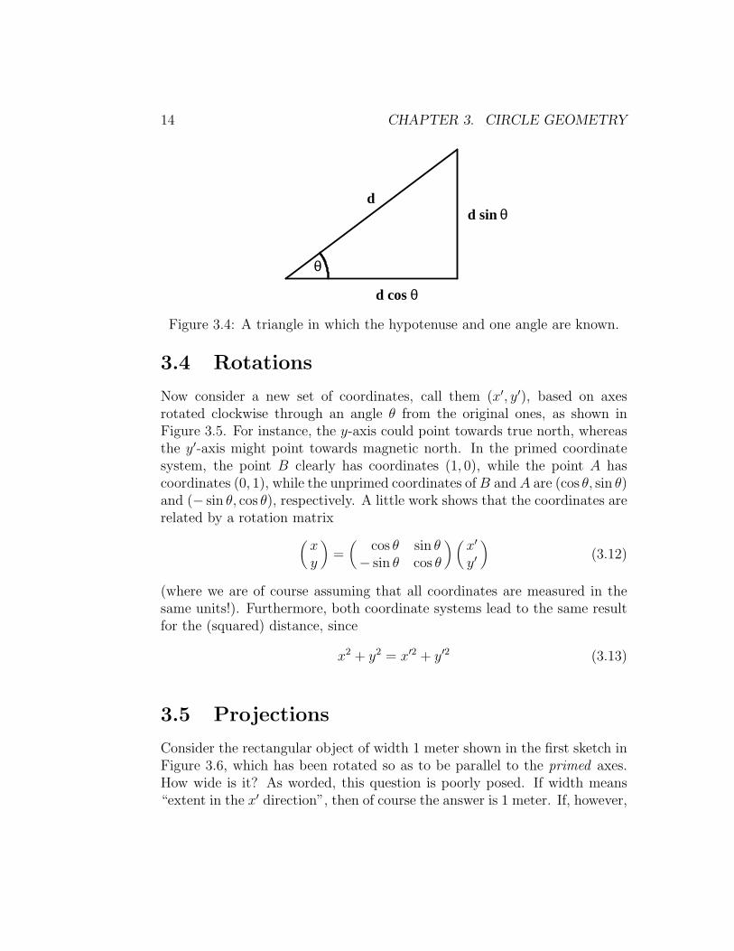
14 CHAPTER 3. CIRCLE GEOMETRY
θd cos
θd sind
θ
Figure 3.4: A triangle in which the hypotenuse and one angle are known.
3.4 Rotations
Now consider a new set of coordinates, call them (x′, y′), based on axesrotated clockwise through an angle θ from the original ones, as shown inFigure 3.5. For instance, the y-axis could point towards true north, whereasthe y′-axis might point towards magnetic north. In the primed coordinatesystem, the point B clearly has coordinates (1, 0), while the point A hascoordinates (0, 1), while the unprimed coordinates of B and A are (cos θ, sin θ)and (− sin θ, cos θ), respectively. A little work shows that the coordinates arerelated by a rotation matrix
(
xy
)
=(
cos θ sin θ− sin θ cos θ
)(
x′
y′
)
(3.12)
(where we are of course assuming that all coordinates are measured in thesame units!). Furthermore, both coordinate systems lead to the same resultfor the (squared) distance, since
x2 + y2 = x′2 + y′2 (3.13)
3.5 Projections
Consider the rectangular object of width 1 meter shown in the first sketch inFigure 3.6, which has been rotated so as to be parallel to the primed axes.How wide is it? As worded, this question is poorly posed. If width means“extent in the x′ direction”, then of course the answer is 1 meter. If, however,

3.6. ADDITION FORMULAS 15
y
B
θ
θ
A
y’
x’
x
Figure 3.5: A rotated coordinate system.
width means “extent in the x direction”, then the answer is obtained bymeasuring the horizontal distance between the sides of the rectangle, whichresults in a value larger than 1. (The exact value is easily seen to be 1/ cos θ.)
Repeat this exercise in the opposite direction. Take the same rectangularobject, but orient it parallel to the unprimed axes, as shown in the secondsketch. How wide is it? Clearly the “unprimed” width is 1 meter, and the“primed” width is larger (and again given by 1/ cos θ).
In one of the cases above, the “primed” width is smaller, yet in the otherthe “unprimed” width is smaller. What is happening here? If you turn yoursuitcase at an angle, it is harder to fit under your seat! It has, in effect,become “longer”! But which orientation is best depends, of course, on theorientation of the seat!
Remember this discussion when we address the corresponding questionsin relativity in subsequent chapters.
3.6 Addition Formulas
Consider the line through the origin which makes an angle φ with the (pos-itive) x-axis, as shown in the first sketch in Figure 3.7. What is its slope?The equation of the line is
y = x tan φ (3.14)
so that slope is tan φ, at least in “unprimed” coordinates. Consider now theline through the origin shown in the second sketch, which makes an angle φ

16 CHAPTER 3. CIRCLE GEOMETRY
θ
1
θ
1
Figure 3.6: Width is coordinate-dependent.
y
xφ
y’
x’
y
x
φθ
Figure 3.7: The addition formula for slopes.
with the (positive) x′-axis. What is its slope? In “primed” coordinates, theequation of the line is just
y′ = x′ tan φ (3.15)
so that, in these coordinates, the slope is again tanφ. But what about in“unprimed” coordinates? The x′ axis itself makes an angle θ with the x-axis.It is tempting to simply add these slopes, obtaining tanφ + tan θ, but thisnot correct. Slopes don’t add; angles do! The correct answer is that
y = x tan(θ + φ) (3.16)
so that the slope is given by (3.8).Remember this discussion when we discuss the Einstein addition law.

Chapter 4
Hyperbola Geometry
In which a 2-dimensional non-Euclidean geometry is constructed, which willturn out to be identical with special relativity.
4.1 Trigonometry
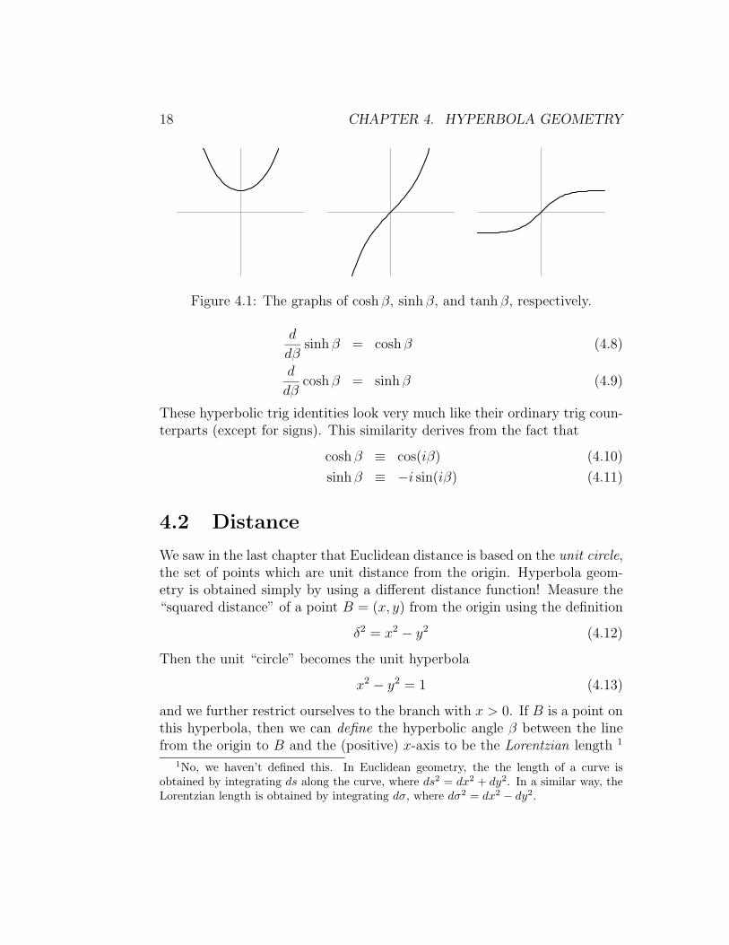
The hyperbolic trig functions are usually defined using the formulas
cosh β =eβ + e−β
2(4.1)
sinh β =eβ − e−β
2(4.2)
and then
tanh β =sinh β
cosh β(4.3)
and so on. We will discuss an alternative definition below. The graphs ofthese functions are shown in Figure 4.1.
It is straightforward to verify from these definitions that
cosh2 β − sinh2 β = 1 (4.4)
sinh(α + β) = sinh α cosh β + cosh α sinh β (4.5)
cosh(α + β) = cosh α cosh β + sinh α sinh β (4.6)
tanh(α + β) =tanh α + tanh β
1 + tanhα tanh β(4.7)
17
18 CHAPTER 4. HYPERBOLA GEOMETRY
Figure 4.1: The graphs of cosh β, sinh β, and tanh β, respectively.
d
dβsinh β = cosh β (4.8)
d
dβcosh β = sinh β (4.9)
These hyperbolic trig identities look very much like their ordinary trig coun-terparts (except for signs). This similarity derives from the fact that
cosh β ≡ cos(iβ) (4.10)
sinh β ≡ −i sin(iβ) (4.11)
4.2 Distance
We saw in the last chapter that Euclidean distance is based on the unit circle,the set of points which are unit distance from the origin. Hyperbola geom-etry is obtained simply by using a different distance function! Measure the“squared distance” of a point B = (x, y) from the origin using the definition
δ2 = x2 − y2 (4.12)
Then the unit “circle” becomes the unit hyperbola
x2 − y2 = 1 (4.13)
and we further restrict ourselves to the branch with x > 0. If B is a point onthis hyperbola, then we can define the hyperbolic angle β between the linefrom the origin to B and the (positive) x-axis to be the Lorentzian length 1
1No, we haven’t defined this. In Euclidean geometry, the the length of a curve isobtained by integrating ds along the curve, where ds2 = dx2 + dy2. In a similar way, theLorentzian length is obtained by integrating dσ, where dσ2 = dx2 − dy2.

4.2. DISTANCE 19
β
βB
y y’
A
x’
x
Figure 4.2: The unit hyperbola. The point A has coordinates (sinh β, cosh β),and B = (cosh β, sinh β).
of the arc of the unit hyperbola between B and the point (1, 0). We couldthen define the hyperbolic trig functions to be the coordinates (x, y) of B,that is
cosh β = x (4.14)
sinh β = y (4.15)
and a little work shows that this definition is exactly the same as the oneabove. 2 This construction is shown in Figure 4.2, which also shows another“unit” hyperbola, given by x2 − y2 = −1. By symmetry, the point A onthis hyperbola has coordinates (x, y) = (sinh β, cosh β). We will discuss theimportance of this hyerbola later.
Many of the features of the graphs shown in Figure 4.1 follow immediatelyfrom this definition of the hyperbolic trig functions in terms of coordinatesalong the unit hyperbola. Since the minimum value of x on this hyperbola
2Use x2 − y2 = 1 to compute
dβ2 ≡ dσ2 = dy2 − dx2 =dx2
x2 − 1=
dy2
y2 + 1
then take the square root of either expression and integrate. (The integrals are hard.)Finally, solve for x or y in terms of β, yielding (4.1) or (4.2), respectively.

20 CHAPTER 4. HYPERBOLA GEOMETRY
4
5
3
β
Figure 4.3: A hyperbolic triangle with tanhβ = 3
5.
is 1, we must have cosh β ≥ 1. As β approaches ±∞, x approaches ∞ and yapproaches ±∞, which agrees with the asymptotic behavior of the graphs ofcosh β and sinh β, respectively. Finally, since the hyperbola has asymptotesy = ±x, we see that | tanh β| < 1, and that tanhβ must approach ±1 as βapproaches ±∞.
So how do we measure the distance between two points? The “squareddistance” was defined in (4.12), and can be positive, negative, or zero! Weadopt the following convention: Take the square root of the absolute valueof the “squared distance”. As we will see in the next chapter, it will alsobe important to remember whether the “squared distance” was positive ornegative, but this corresponds directly to whether the distance is “mostlyhorizontal” or “mostly vertical”.
4.3 Triangle Trig
We now recast ordinary triangle trig into hyperbola geometry.
Suppose you know tanhβ = 3
5, and you wish to determine cosh β. One
can of course do this algebraically, using the identity
cosh2 β =1
1 − tanh2 β(4.16)
But it is easier to draw any triangle containing an angle whose hyperbolictangent is 3
5. In this case, the obvious choice would be the triangle shown in
Figure 4.3, with sides of 3 and 5.

4.4. ROTATIONS 21
βd cosh
βd sinhd
β
Figure 4.4: A hyperbolic triangle in which the hypotenuse and one angle areknown.
What is cosh β? Well, we first need to work out the length δ of thehypotenuse. The (hyperbolic) Pythagorean Theorem tells us that
52 − 32 = δ2 (4.17)
so δ is clearly 4. Take a good look at this 3-4-5 triangle of hyperbola geometry,which is shown in Figure 4.3! But now that we know all the sides of thetriangle, it is easy to see that coshβ = 5
4.
Trigonometry is not merely about ratios of sides, it is also about projec-tions. Another common use of triangle trig is to determine the sides of atriangle given the hypotenuse d and one angle β. The answer, of course, isthat the sides are d cosh β and d sinh β, as shown in in Figure 4.4.
4.4 Rotations
By analogy with the Euclidean case, we define a hyperbolic rotation throughthe relations
(
x
y
)
=
(
cosh β sinh β
sinh β cosh β
)(
x′
y′
)
(4.18)
This corresponds to “rotating” both the x and y axes into the first quadrant,as shown in Figure 4.2. While this may seem peculiar, it is easily verifiedthat the “distance” is invariant, that is,
x2 − y2 ≡ x′2 − y′2 (4.19)
which follows immediately from the hyperbolic trig identity (4.4).

22 CHAPTER 4. HYPERBOLA GEOMETRY
4.5 Projections
We can ask the same question as we did for Euclidean geometry. Considera rectangle of width 1 whose sides are parallel to the unprimed axes. Howwide is it when measured in the primed coordinates? It turns out that thewidth of the box in the primed coordinate system is less than 1. This islength contraction, to which we will return in the next chapter, along withtime dilation.
4.6 Addition Formulas
What is the slope of the line from the origin to the point A in Figure 4.2?The equation of this line, the y′-axis, is
x = y tanh β (4.20)
Consider now a line with equation
x′ = y′ tanh α (4.21)
What is its (unprimed) slope? Again, slopes don’t add, but (hyperbolic)angles do; the answer is that
x = y tanh(α + β) (4.22)
which can be expressed in terms of the slopes tanh α and tanh β using (4.7).As discussed in more detail in the next chapter, this is the Einstein additionformula!

Chapter 5
The Geometry of
Special Relativity
In which it is shown that special relativity is just hyperbolic geometry.
5.1 Spacetime Diagrams
A brilliant aid in understanding special relativity is the Surveyor’s parableintroduced by Taylor and Wheeler [1, 2]. Suppose a town has daytime sur-veyors, who determine North and East with a compass, nighttime surveyors,who use the North Star. These notions of course differ, since magnetic northis not the direction to the North Pole. Suppose further that both groupsmeasure north/south distances in miles and east/west distances in meters,with both being measured from the town center. How does one go aboutcomparing the measurements of the two groups?
With our knowledge of Euclidean geometry, we see how to do this: Con-vert miles to meters (or vice versa). Furthermore, distances computed withthe Pythagorean theorem do not depend on which group does the surveying.Finally, it is easily seen that “daytime coordinates” can be obtained from“nighttime coordinates” by a simple rotation. The moral of this parable istherefore:
1. Use the same units.
2. The (squared) distance is invariant.
3. Different frames are related by rotations.
23

24 CHAPTER 5. THE GEOMETRY OF SPECIAL RELATIVITY
Applying that lesson to relativity, the first thing to do is to measure bothtime and space in the same units. How does one measure distance in seconds?that’s easy: simply multiply by c. Thus, since c = 3 × 10⁸ m
s, 1 second of
distance is just 3 × 10⁸ m. 1 Note that this has the effect of setting c = 1,since the number of seconds (of distance) traveled by light in 1 second (oftime) is precisely 1.
Of course, it is also possible to measure time in meters: simply divideby c. Thus, 1 meter of time is the time it takes for light (in vacuum) totravel 1 meter. Again, this has the effect of setting c = 1.
5.2 Lorentz Transformations
The Lorentz transformation between a frame (x, t) at rest and a frame (x′, t′)moving to the right at speed v was derived in Chapter 2. The transformationfrom the moving frame to the frame at rest is given by
x = γ (x′ + vt′) (5.1)
t = γ(
t′ +v
c2x′)
(5.2)
where
γ =1
√
1 − v2
c2
(5.3)
The key to converting this to hyperbola geometry is to measure space andtime in the same units by replacing t by ct. The transformation from themoving frame, which we now denote (x′, ct′), to the frame at rest, now de-noted (x, ct), is given by
x = γ (x′ +v
cct′) (5.4)
ct = γ(
ct′ +v
cx′)
(5.5)
which makes the symmetry between these equations much more obvious.We can simplify things still further. Introduce the rapidity β via 2
v
c= tanh β (5.6)
1A similar unit of distance is the lightyear, namely the distance traveled by light in 1year, which would here be called simply a year of distance.
2WARNING: Some authors use β for v
c, not the rapidity.

5.2. LORENTZ TRANSFORMATIONS 25
β
βB
t’
A
x’
t
x
Figure 5.1: The Lorentz transformation between an observer at rest and anobserver moving at speed v
c= c tanh β is shown as a hyperbolic rotation. The
point A has coordinates (sinh β, cosh β), and B = (cosh β, sinh β). (Unitshave been chosen such that c = 1.)
Inserting this into the expression for γ we obtain
γ =1
√
1 − tanh2 β=
√
√
√
√
cosh2 β
cosh2 β − sinh2 β= cosh β (5.7)
andv
cγ = tanh β cosh β = sinh β (5.8)
Inserting these identities into the Lorentz transformations above brings themto the remarkably simple form
x = x′ cosh β + ct′ sinh β (5.9)
ct = x′ sinh β + ct′ cosh β (5.10)
which in matrix form are just
(
x
ct
)
=
(
cosh β sinh β
sinh β cosh β
)(
x′
ct′
)
(5.11)
But (5.11) is just (4.18), with y = ct!

26 CHAPTER 5. THE GEOMETRY OF SPECIAL RELATIVITY
Thus, Lorentz transformations are just hyperbolic rotations! As noted inthe previous chapter, the invariance of the interval follows immediately fromthe fundamental hyperbolic trig identity (4.4). This invariance now takes theform
x2 − c2t2 ≡ x′2 − c2t′2 (5.12)
We thus have precisely the situation described in Figure 4.2, but with yreplaced by ct; this is shown in Figure 5.1.
5.3 Space and Time
We now return to the peculiar fact that the “squared distance” between twopoints can be positive, negative, or zero. This sign is positive for horizontaldistances and negative for vertical distances. But these directions correspondto the coordinates x and t, and measure space and time, respectively — asseen by the given observer. But any observer’s space axis must intersectthe unit hyperbola somewhere, and hence corresponds to positive “squareddistance”. Such directions have more space than time, and will be calledspacelike. Similarly, any observer’s time axis intersects the hyperbola x2 −c2t2 = −1, corresponding to negative “squared distance”; such directions aretimelike.
What about diagonal lines at a (Euclidean!) angle of 45◦? These corre-spond to a “squared distance” of zero — and to moving at the speed of light.All observers agree about these directions, which will be called lightlike. Inhyperbola geometry, there are thus preferred directions of “length zero”. In-deed, this is the geometric realization of the idea that the speed of light isthe same for all observers!
It is important to realize that every spacelike direction corresponds to thespace axis for some observer. Events separated by a spacelike line occur atthe simultaneously for that observer — and the (square root of the) “squareddistance” is just the distance between the events as seen by that observer.Similarly, events separated by a timelike line occur at the same place forsome observer, and the (square root of −1 times the) “squared distance” isjust the time which elapses between the events as seen by that observer.
On the other hand, events separated by a timelike line do not occur simul-taneously for any observer! We can thus divide the spacetime diagram intocausal regions as follows: Those points connected to the origin by spacelikelines occur “now” for some observer, whereas those points connected to the

5.4. DOT PRODUCT 27
nownow
past
future
Figure 5.2: The causal relationship between points in spacetime and theorigin.
origin by timelike lines occur unambiguously in the future or the past. Thisis shown in Figure 5.2. 3
In order to be able to make sense of cause and effect, only events in ourpast can influence us, and we can only influence events in our future. Putdifferently, if information could travel faster than the speed of light, thendifferent observers would no longer be able to agree on cause and effect.
5.4 Dot Product
In Euclidean geometry, distances can be described by taking the (squared!)length of a vector using the dot product. Denoting the unit vectors in the xand y directions by x and y, respectively, then the vector from the origin tothe point (x, y) is just
~r = x x + y y (5.13)
whose (squared) length is just
|~r|2 = ~r ·~r = x2 + y2 (5.14)
It is straightforward to generalize this to hyperbola geometry. Denote theunit vectors in the t and x directions by t and x. 4 Then the (Lorentzian)
3With two or more spatial dimensions, the lightlike directions would form a surfacecalled the light cone, and the regions labeled “now” would be connected.
4Unit vectors are dimensionless! It is neither necessary nor desirable to include a factorof c in the definition of t.
28 CHAPTER 5. THE GEOMETRY OF SPECIAL RELATIVITY
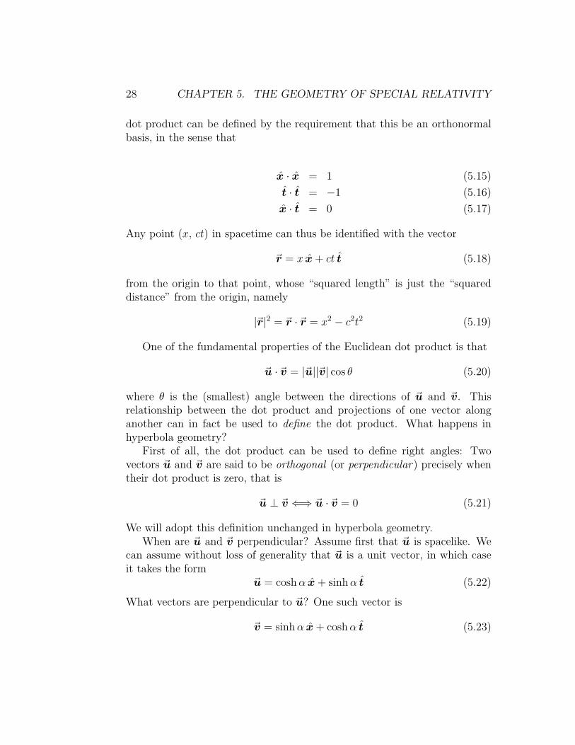
dot product can be defined by the requirement that this be an orthonormalbasis, in the sense that
x · x = 1 (5.15)
t · t = −1 (5.16)
x · t = 0 (5.17)
Any point (x, ct) in spacetime can thus be identified with the vector
~r = x x + ct t (5.18)
from the origin to that point, whose “squared length” is just the “squareddistance” from the origin, namely
|~r|2 = ~r ·~r = x2 − c2t2 (5.19)
One of the fundamental properties of the Euclidean dot product is that
~u · ~v = |~u||~v| cos θ (5.20)
where θ is the (smallest) angle between the directions of ~u and ~v. Thisrelationship between the dot product and projections of one vector alonganother can in fact be used to define the dot product. What happens inhyperbola geometry?
First of all, the dot product can be used to define right angles: Twovectors ~u and ~v are said to be orthogonal (or perpendicular) precisely whentheir dot product is zero, that is
~u ⊥ ~v ⇐⇒ ~u · ~v = 0 (5.21)
We will adopt this definition unchanged in hyperbola geometry.When are ~u and ~v perpendicular? Assume first that ~u is spacelike. We
can assume without loss of generality that ~u is a unit vector, in which caseit takes the form
~u = cosh α x + sinh α t (5.22)
What vectors are perpendicular to ~u? One such vector is
~v = sinh α x + cosh α t (5.23)

5.4. DOT PRODUCT 29
and it is easy to check that all other solutions are multiples of this one. Notethat ~v is timelike! Had we assumed instead that ~v were timelike, we wouldmerely have interchanged the roles of ~u and ~v.
Furthermore, ~u and ~v are just the space and time axes, respectively, of anobserver moving with speed v
c= tanh α. So orthogonal directions correspond
precisely to the coordinate axes of some observer.What if ~u is lightlike? It is a peculiarity of Lorentzian (hyperbola) ge-
ometry that there are nonzero vectors of length zero. But since the dotproduct gives the length, having length zero means that lightlike vectors areperpendicular to themselves!
We can finally define the length of a vector ~v by
|~v| =√
|~v · ~v| (5.24)
If ~v is spacelike we can write
~v = |~v|(cosh α x + sinh α t) (5.25)
while if ~v is timelike we can write
~v = |~v|(sinh α x + cosh α t) (5.26)
(If ~v is lightlike, |~v| = 0, so no such expression exists.)The above argument shows that timelike vectors can only be perpendicu-
lar to spacelike vectors, and vice versa. We will also say in this case that thevectors form a right angle. Recall that hyperbolic angles were defined alongthe unit hyperbola, hence only exist (as originally defined) between spacelikedirections! It is straightforward to extend this to timelike directions usingthe hyperbola x2 − ct2 = −1; this was implicitly done when drawing Fig-ure 4.2. But there is no hyperbola relating timelike directions to spacelikeones. Thus, a “right angle” isn’t an angle at all!
A right triangle is one which contains a right angle. By the above dis-cussion, one of the legs of such a triangle must be spacelike, and the othertimelike. Consider first the case where the hypotenuse is either spacelike ortimelike. The only hyperbolic angle in such a triangle is the one between thehypotenuse and the leg of the same type, that is between the two timelikesides if the hypotenuse is timelike, and between the two spacelike sides if thehypotenuse is spacelike. Several such hyperbolic right triangles are shown inFigures 5.3. It is also possible for the hypotenuse to be null, as shown inFigure 5.4. Such triangles do not have any hyperbolic angles!

30 CHAPTER 5. THE GEOMETRY OF SPECIAL RELATIVITY
5 4
3
β
5
4
3
α
4
5
3
α
4
5
3
β
Figure 5.3: Some hyperbolic right triangles.
Figure 5.4: More hyperbolic right triangles. The right angle is on the left!
What happens if we take the dot product between two spacelike vectors?We can assume without loss of generality that one vector is parallel to the xaxis, in which case we have
~u = |~u| x (5.27)
~v = |~v|(cosh α x + sinh α t) (5.28)
so that the dot product satisfies
~u · ~v = |~u||~v| cosh α (5.29)
What happens if both vectors are timelike? The above argument still works,except that the roles of x and t must be interchanged, resulting in
~u · ~v = −|~u||~v| cosh α (5.30)
In both cases, note that |~v| cosh α is the projection of ~v along ~u; see Fig-ure 5.5.
But what happens if we take the dot product between a timelike vectorand a spacelike vector? We can again assume without loss of generality thatthe spacelike vector is parallel to the x axis, so that
~u = |~u| x (5.31)
~v = |~v|(sinh α x + cosh α t) (5.32)

5.4. DOT PRODUCT 31
�����������
α
~v−~v · ~u|~u|
��
��
��
��>
α
~v
~v · ~u|~u|
Figure 5.5: Hyperbolic projections between two spacelike vectors, or betweentwo timelike vectors.
�����������
α~v
~v · ~u|~u|
��
��
��
��>
α
~v −~v · ~u|~u|
Figure 5.6: Hyperbolic projections between timelike and spacelike vectors.
The dot product now satisfies
~u · ~v = |~u||~v| sinh α (5.33)
At first sight, this is something new. But note from the first drawing inFigure 5.6 that ~v sinh α is just the projection of ~v along ~u! The new featurehere is that we can’t define the angle between a timelike direction and aspacelike direction. The only angle in the triangle which is defined is the oneshown! 5
5Alternatively, we could have assumed that the timelike vector was parallel to the t
axis, resulting in the second drawing in Figure 5.6. The conclusion is the same, althoughnow it represents the projection of ~u along ~v.

32 CHAPTER 5. THE GEOMETRY OF SPECIAL RELATIVITY

Chapter 6
Applications
6.1 Addition of Velocities
What is the rapidity β? Consider an observer moving at speed v to the right.This observer’s world line intersects the unit hyperbola
c2t2 − x2 = 1 (ct > 0) (6.1)
at the point A = (sinh β, cosh β); this line has “slope” 1
v
c= tanh β (6.2)
as required. Thus, β can be thought of as the hyperbolic angle between thect-axis and the worldline of a moving object. As discussed in the precedingchapter, β turns out to be precisely the distance from the axis as measuredalong the hyperbola (in hyperbola geometry!). This was illustrated in Fig-ure 5.1.
Consider therefore an object moving at speed u relative to an observermoving at speed v. Their rapidities are given by
u
c= tanh α (6.3)
v
c= tanh β (6.4)
1It is not obvious whether “slope” should be defined by ∆x
c ∆tor by the reciprocal of
this expression. This is further complicated by the fact that both (x, ct) and (ct, x) arecommonly used to denote the coordinates of the point A!
33

34 CHAPTER 6. APPLICATIONS
x’
t’t
x
x’
t’t
x
Figure 6.1: Length contraction as a hyperbolic projection.
To determine the resulting speed with respect to an observer at rest, simplyadd the rapidities ! One way to think of this is that you are adding the arclengths along the hyperbola. Another is that you are following a (hyperbolic)rotation through a (hyperbolic) angle β (to get to the moving observer’sframe) with a rotation through an angle α. In any case, the resulting speedw is given by
w
c= tanh(α + β) =
tanh α + tanh β
1 + tanh α tanh β=
uc
+ vc
1 + uvc2
(6.5)
which is — finally — precisely the Einstein addition formula!
6.2 Length Contraction
We now return to the question of how “wide” things are.Consider first a meter stick at rest. In spacetime, the stick “moves”
vertically, that is, it ages. This situation is shown in the first sketch inFigure 6.1, where the horizontal lines show the meter stick at various times(according to an observer at rest). How “wide” is the worldsheet of the stick?The observer at rest of course measures the length of the stick by locatingboth ends at the same time, and measuring the distance between them. Att = 0, this corresponds to the 2 heavy dots in the sketch, one at the originand the other on the unit hyperbola. But all points on the unit hyperbolaare at an interval of 1 meter from the origin. The observer at rest thereforeconcludes, unsurprisingly, that the meter stick is 1 meter long.

6.3. TIME DILATION 35
How long does a moving observer think the stick is? This is just the“width” of the worldsheet as measured by the moving observer. This observerfollows the same procedure, by locating both ends of the stick at the sametime, and measuring the distance between them. But time now correspondsto t′, not t. At t′ = 0, this measurement corresponds to the heavy line in thesketch. Since this line fails to reach the unit hyperbola, it is clear that themoving observer measures the length of a stationary meter stick to be lessthan 1 meter. This is length contraction.
To determine the exact value measured by the moving observer, computethe intersection of the line x = 1 (the right-hand edge of the meter stick)with the line t′ = 0 (the x′-axis), or equivalently ct = x tanh β, to find that
ct = tanh β (6.6)
so that x′ is just the interval from this point to the origin, which is
x′ =√
x2 − c2t2 =√
1 − tanh2 β =1
cosh β(6.7)
What if the stick is moving and the observer is at rest? This situation isshown in the second sketch in Figure 6.1. The worldsheet now correspondsto a “rotated rectangle”, indicated by the parallelograms in the sketch. Thefact that the meter stick is 1 meter long in the moving frame is shown bythe distance between the 2 heavy dots (along t′ = 0), and the measurementby the observer at rest is indicated by the heavy line (along t = 0). Again,it is clear that the stick appears to have shrunk, since the heavy line fails toreach the unit hyperbola.
Thus, a moving object appears shorter by a factor 1/ cosh β. It doesn’tmatter whether the stick is moving, or the observer; all that matters is theirrelative motion.
6.3 Time Dilation
We now investigate moving clocks. Consider first the smaller dot in Fig-ure 6.2. This corresponds to ct = 1 (and x = 0), as evidenced by the factthat this point is on the (other) unit hyperbola, as shown. Similarly, thelarger dot, lying on the same hyperbola, corresponds to ct′ = 1 (and x′ = 0).The horizontal line emanating from this dot gives the value of ct there, which

36 CHAPTER 6. APPLICATIONS
x’
t’t
x
Figure 6.2: Time dilation as a hyperbolic projection.
is clearly greater than 1. This is the time measured by the observer at restwhen the moving clock says 1; the moving clock therefore runs slow. But nowconsider the diagonal line emanating from the larger dot. At all points alongthis line, ct′ = 1. In particular, at the smaller dot we must have ct′ > 1. Thisis the time measured by the moving observer when the clock at rest says 1;the moving observer therefore concludes the clock at rest runs slow!
There is no contradiction here; one must simply be careful to ask theright question. In each case, observing a clock in another frame of referencecorresponds to a projection. In each case, a clock in relative motion to theobserver appears to run slow.
6.4 Doppler Shift
The frequency f of a beam of light is related to its wavelength λ by theformula
fλ = c (6.8)
How do these quantities depend on the observer?
Consider an inertial observer moving to the right in the laboratory framewho is carrying a flashlight that is pointing to the left; see Figure 6.3. Thenthe moving observer is traveling along a path of the form x′ = x′
1 = const.Suppose the moving observer turns on the flashlight (at time t′1) just longenough to emit 1 complete wavelength of light, and that this takes time dt′.

6.4. DOPPLER SHIFT 37
1 1
1
0 0
10 1(t +dt ,x +dx )
(t ,x )
1
(t +dt ,0)
(t ,0)
Figure 6.3: The Doppler effect: An observer moving to the right emits apulse of light to the left, which is later seen by a stationary observer. Thewavelengths measured by the two observers differ, causing a Doppler shift inthe frequency.
Then the moving observer “sees” a wavelength
λ′ = c dt′ (6.9)
According to the lab, the flashlight was turned on at the event (t1, x1),and turned off dt1 seconds later, during which time the moving observermoved a distance dx1 meters to the right. But when was the light received,at x = 0, say?
Let (t0, 0) denote the first reception of light by a lab observer at x = 0,and suppose this observer sees the light stay on for dt0 seconds. Since lighttravels at the speed of light, we have the equations
c(t0 − t1) = x1 (6.10)
c[(t0 + dt0) − (t1 + dt1)] = x1 + dx1 (6.11)
from which it follows that
c(dt0 − dt1) = dx1 (6.12)
so that
c dt0 = dx1 + c dt1 (6.13)
= (dx′1 cosh β + c dt′1 sinh β) + (c dt′1 cosh β + dx′
1 sinh β) (6.14)
= (cosh β + sinh β) c dt′1 (6.15)

38 CHAPTER 6. APPLICATIONS
since dx′1 = 0. But the wavelength as seen in the lab is
λ = c dt0 (6.16)
so that
λ
λ′=
dt0dt′1
= cosh β + sinh β
= cosh β (1 + tanh β) = γ(
1 +v
c
)
=
√
√
√
√
1 + vc
1 − vc
(6.17)
The frequencies transform inversely, that is
f ′
f=
√
√
√
√
1 + vc
1 − vc
(6.18)

Chapter 7
Problems I
7.1 Cosmic Rays
Consider µ-mesons produced by the collision of cosmic rays with gas nucleiin the atmosphere 60 kilometers above the surface of the earth, which thenmove vertically downward at nearly the speed of light. The half-life beforeµ-mesons decay into other particles is 1.5 microseconds (1.5 × 10⁻⁶ s).
1. Assuming it doesn’t decay, how long would it take a µ-meson to reachthe surface of the earth?
2. Assuming there were no time dilation, approximately what fraction ofthe mesons would reach the earth without decaying?
3. In actual fact, roughly 1
8of the mesons would reach the earth! How fast
are they going?
1. Without much loss of accuracy, assume the mesons travel at the speed oflight. Then it takes them
60 km
3 × 10⁸ ms
= 200 µs (7.1)
2. 200 µs is200
1.5=
400
3half-lives, so only 2−
4003 of the mesons reach the
earth!
39
40 CHAPTER 7. PROBLEMS I
9400
α
400
9
α
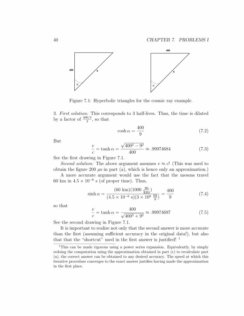
Figure 7.1: Hyperbolic triangles for the cosmic ray example.
3. First solution: This corresponds to 3 half-lives. Thus, the time is dilatedby a factor of 400/3
3, so that
cosh α =400
9(7.2)
Butv
c= tanh α =
√4002 − 92
400≈ .99974684 (7.3)
See the first drawing in Figure 7.1.Second solution: The above argument assumes v ≈ c! (This was used to
obtain the figure 200 µs in part (a), which is hence only an approximation.)A more accurate argument would use the fact that the mesons travel
60 km in 4.5 × 10⁻⁶ s (of proper time). Thus,
sinh α =(60 km)(1000 m
km)
(4.5 × 10⁻⁶ s)(3 × 10⁸ ms )
=400
9(7.4)
so thatv
c= tanh α =
400√4002 + 92
≈ .99974697 (7.5)
See the second drawing in Figure 7.1.It is important to realize not only that the second answer is more accurate
than the first (assuming sufficient accuracy in the original data!), but alsothat that the “shortcut” used in the first answer is justified! 1
1This can be made rigorous using a power series expansion. Equivalently, by simplyredoing the computation using the approximation obtained in part (c) to recalculate part(a), the correct answer can be obtained to any desired accuracy. The speed at which thisiterative procedure converges to the exact answer justifies having made the approximationin the first place.

7.2. DOPPLER EFFECT 41
2
2
4
4
α
2
x
x
4-x
α
Figure 7.2: Computing Doppler shift.
7.2 Doppler Effect
1. A rocket sends out flashes of light every 2 seconds in its own rest frame,which you receive every 4 seconds. How fast is the rocket going?
1. First solution: This situation is shown in the first drawing in Figure 7.2.In order to find the hyperbolic angle α, draw a horizontal line as shown inthe enlarged second drawing, resulting in the system of equations 2
tanh α =x
4 − x(7.7)
(4 − x)2 − x2 = 22 (7.8)
which is easily solved for x = 3
2, so that v
c= tanh α = 3
5.
Second solution: Insert λ = 4 and λ′ = 2 into (6.17), and solve for vc.
2This method can be be used to derive the Doppler shift formula in general, yielding
v
c=
λ2 − λ′2
λ2 + λ′2(7.6)
which is equivalent to (6.17); in this example, λ = 4 and λ′ = 2.

42 CHAPTER 7. PROBLEMS I

Chapter 8
Paradoxes
In which impossible things are shown to be possible.
8.1 Special Relativity Paradoxes
It is easy to create seemingly impossible scenarios in special relativity byplaying on the counterintuitive nature of observer-dependent time. Thesescenarios are usually called paradoxes, because they seem to be impossible.Yet there is nothing paradoxical about them!
The best way to resolve these so-called paradoxes is to draw a good space-time diagram. This requires careful reading of the problem, making surealways to associate the given information with a particular reference frame.A single spacetime diagram suffices to determine what all observers see. Itis nevertheless instructive to draw separate spacetime diagrams for each ob-server, making sure that they all agree.
In this chapter, we discuss the two most famous paradoxes in specialrelativity, the Pole and Barn Paradox and the Twin Paradox. We also brieflydiscuss the more subtle aspects of flying manhole covers.
8.2 The Pole and Barn Paradox
A 20 foot pole is moving towards a 10 foot barn fast enough that the poleappears to be only 10 feet long. As soon as both ends of the pole are in thebarn, slam the doors. How can a 20 foot pole fit into a 10 foot barn?
43

44 CHAPTER 8. PARADOXES
-20
-10
0
10
20
-20 -10 10 20 30
-20
-10
0
10
20
-10 10 20 30
BARN POLE
Figure 8.1: In each diagram, the heavy straight lines represent the ends ofthe pole and the lighter straight lines represent the front and back of thebarn. The hyperbolas of “radius” 10 and 20 are also shown. The dot at theorigin labels the event where the back of the pole enters the barn, and theother dot labels the event where the front of the pole leaves the barn.
This is the beginning of the Pole and Barn Paradox. It’s bad enoughtrying to imagine what happens to the pole when it suddenly stops and findsitself in a barn which is too small. But what does the pole see?
Since length contraction is symmetric, if the barn sees the pole shortenedby a factor of 2, then the pole sees the barn shortened by the same factorof 2. This factor is just cosh β, where |β| is the same in both cases. So the20 foot pole sees this 5 foot barn approaching. No way is the pole going tofit in the barn!
So what does the pole see?
The spacetime diagrams for this situation are shown in Figure 8.1, asseen first from the barn’s reference frame and then from the pole’s referenceframe. The 2 dots represent the events of closing the barn doors when theends of the pole are even with the corresponding door.
In the barn’s frame, these events happen simultaneously, so it is possiblein principle to trap the pole in the barn by shutting the doors “at the sametime”. (We omit speculation about what happens when the pole hits theclosed door!)
In the pole’s frame, the exit door is closed long before the rear of the poleenters the barn. Assuming the pole keeps going, for instance by virtue of

8.3. THE TWIN PARADOX 45
the door opening again, then the entrance door is closed much later, whenthe rear of the pole finally gets there. The pole thinks it silly to try to catchit by waiting to close the entrance door until most of the pole has alreadyescaped through the exit door!
8.3 The Twin Paradox
One twin travels 24 light-years to star X at speed 24
25c; her twin brother stays
home. When the traveling twin gets to star X, she immediately turns around,and returns at the same speed. How long does each twin think the trip took?
Star X is 24 light-years away, so, according to the twin at home, it takesher 25 years to get there, and 25 more to return, for a total of 50 years awayfrom earth. But the traveling twin’s clock runs slow by a actor of
cosh β =1
1 − tanh2 β=
25
7
This means that, according to the traveling twin, it only takes her 7 yearseach way. Thus, she has only aged 14 years while her brother has aged 50!
This is in fact correct, and represents a sort of time travel into the future:It only takes the traveling twin 14 years to get 50 years into earth’s future.(Unfortunately, there’s no way to get back!)
But wait a minute. The traveling twin should see her brother’s clock runslow, by the same factor of 25
7. So when 7 years of her time elapse, she thinks
her brother has only aged 49
25≈ 2 years! Her brother should therefore only
have aged 4 years when she returns!
This can’t be right. Either her brother is 4 years older, or he is 50 yearsolder. Both siblings must surely agree on that!
The easiest way to resolve this is to draw a single spacetime diagramshowing the entire trip in the reference frame of the stay-at-home twin, asshown in Figure 8.2. The lower half of the figure is a hyperbolic triangle withtanh β = 24
25, and hypotenuse 7 years. The remaining diagonal lines are lines
of constant time for the traveling twin, at the point of turnaround, whilegoing and returning, respectively. There is another right trangle containingthe hyperbolic angle β; the right angle is at the point of turnaround, and thehypotenuse is 7
cosh β= 49
25years, the age of the stay-at-home twin “when” the
traveling twin turns around.

46 CHAPTER 8. PARADOXES
49/25
7
24
25
β
Figure 8.2: The spacetime diagram for the Twin Paradox. The vertical linerepresents the world line of the stay-at-home twin, while the heavy diagonallines show the world line of the traveling twin.
How much does each twin age? Simply measure the length of their worldlines! Intervals are invariant; it doesn’t matter how you compute them. Theclear answer is that the brother has indeed aged 50 years, while the sisterhas only aged 14 years.
So what was wrong with the argument that the brother should haveonly aged 4 years? There are really 3 reference frames here: earth, going,and returning. The “going” and “returning” frames yield different times onearth for the turnaround — and these times differ by precisely 1152
25≈ 46
years! From this point of view, it takes the traveling twin 46 years to turnaround!
One difference between the twins is that the traveling twin is not in aninertial frame — she is in 2 inertial frames, but must accelerate in order toswitch from one to the other. This breaks the symmetry between the 2 twins.
However, this is not really the best way to explain this paradox. It ispossible to remove this particular asymmetry by assuming the universe isclosed, so that the traveling twin doesn’t need to turn around! A simplifiedversion of this is to put the problem on a cylinder [4]. It turns out that thisintroduces another sort of asymmetry, but there is a simpler way to lookat it.
The amount an observer ages is just the timelike interval measured alonghis or her worldline. We used this argument above. This approach also worksfor curved worldlines, corresponding to noninertial observers — except that

8.4. MANHOLE COVERS 47
one must integrate the infinitesimal timelike interval dτ =√
dt2 − ds2 alongthe worldline.
A little thought leads to the following remarkable result: The timelikeline connecting 2 events (assuming there is one) is the longest path fromone to the other. (Think about it. Use this line as the t axis. Then any otherpath has a nonzero contribution from the change in x — which decreases thehyperbolic length of the path, and hence the time taken.)
8.4 Manhole Covers
There are 2 well-known paradoxes involving manhole covers, which illustratesome unexpected implications of special relativity. In the first, a 2 footmanhole cover approaches a 2 foot manhole at relativistic velocity. Since thehole sees the cover as much smaller than 2 feet long, the cover must fall intothe manhole. It does.
But what does the cover see? It sees a very small hole rushing at it. Noway is this enormous manhole cover going to fit into this small hole!
The resolution of this paradox requires careful consideration of what itmeans for the something to begin to fall, and is left to the reader.
There is also a higher-dimensional version of this problem, without thecomplication of falling, that is, without gravity. Suppose the manhole coveris flying to the right as before, but now the hole is in a metal sheet which isrising up to meet it. Again, from the point of view of the hole, the cover isvery small and so — if the timing is right — the cover will pass through thehole. It does.
But what does the cover see? It again sees a very small hole rushing atit. How do you get a big object through a small hole? This time one mustconsider what it means for the cover to “pass through” the whole.
If you have successfully resolved these 2 paradoxes, you will realize thatsome properties of materials which we take for granted will are quite impos-sible in special relativity!

48 CHAPTER 8. PARADOXES

Chapter 9
Relativistic Mechanics
In which it is shown that mass is energy.
9.1 Proper Time
In the rest frame, position doesn’t change. Let τ denote “wristwatch time”[2], that is, time as measured by a clock carried by an observer moving atconstant speed u with respect to the given frame. In the moving observer’srest frame, position doesn’t change. We therefore have
(∆x)2 − c2(∆t)2 = 0 − c2(∆τ)2 (9.1)
so that
(∆τ)2 =
(
1 − 1
c2
(
∆x
∆t
)2)
(∆t)2 (9.2)
or equivalently
dτ =
√
1 − u
c2dt =
1
γdt =
1
cosh αdt (9.3)
Note that proper time is independent of reference frame!
9.2 Energy and Momentum
Consider the ordinary velocity of a moving object, defined by
u =d
dtx (9.4)
49

50 CHAPTER 9. RELATIVISTIC MECHANICS
This transforms in a complicated way, since
1
c
dx′
dt′=
1
cdxdt
− vc
1 − vc2
dxdt
(9.5)
The reason for this is that both the numerator and the denominator needto be transformed. The invariance of proper time suggests that we shouldinstead differentiate with respect to proper time, since of course
d
dτx′ =
dx
dτ(9.6)
or in other words since the operator ddτ
pulls through the Lorentz transfor-mation, so that only the numerator is transformed when changing referenceframes.
Furthermore, the same argument can be applied to t, which suggeststhat there are (in 2 dimensions) 2 components to the velocity. We thereforeconsider the “2-velocity”
u =d
dτ
(
ctx
)
=
(
c dtdτdxdτ
)
(9.7)
But sincedt = cosh α dτ (9.8)
anddx2 − c2dt2 = −c2dτ 2 (9.9)
we also havedx = c sinh α dτ (9.10)
so that
u = c(
cosh αsinh α
)
(9.11)
Note that 1
cu is a unit vector, that is
1
c2u · u = 1 (9.12)
and further thatu
c=
dx
dt= tanh α (9.13)
as expected.

9.3. CONSERVATION LAWS 51
9.3 Conservation Laws
Suppose that (Newtonian) momentum is conserved in a given frame, that is∑
mivi =∑
mj vj (9.14)
(Both of these would be 0 in the center-of-mass frame.) Changing to anotherframe moving with respect to the first at speed v, we have
vi = v′i + v (9.15)
vj = v′j + v (9.16)
so that∑
mi(v′i + v) =
∑
mj(v′j + v) (9.17)
We therefore see that∑
miv′i =
∑
mj v′j ⇐⇒
∑
mi =∑
mj (9.18)
that is, momentum is conserved in all inertial frames provided it is conservedon one frame and mass is conserved.
Repeating the computation for the kinetic energy, we obtain starting from
1
2
∑
miv2i =
1
2
∑
mj v2j (9.19)
that1
2
∑
mi(v′i + v)2 =
1
2
∑
mj(v′j + v)2 (9.20)
Expanding this out, we discover that (kinetic) energy is conserved in allframes provided it is conserved in one frame and both mass and momentumare conserved.
The situation in special relativity is quite different.Consider first the momentum defined by the ordinary velocity, namely
p = mu = mdx
dt(9.21)
This momentum is not conserved!We use instead the momentum defined by the 4-velocity, which is given
by
p = mdx
dτ= mc sinh α (9.22)

52 CHAPTER 9. RELATIVISTIC MECHANICS
Suppose now that, as seen in a particular inertial frame, the total momentumof a collection of particles is the same before and after some interaction, thatis
∑
mic sinh αi =∑
mjc sinh αj (9.23)
Consider now the same situation as seen by another inertial referenceframe, moving with respect to the first with speed
v = c tanh β (9.24)
We therefore have
αi = α′i + β (9.25)
αj = α′j + β (9.26)
Inserting this into the conservation rule (9.23) leads to∑
mic sinh α′i =
∑
mic sinh(αi − β) (9.27)
=(
∑
mic sinh αi
)
cosh β −(
∑
mic cosh αi
)
sinh β (9.28)
and similarly∑
mjc sinh α′j =
(
∑
mjc sinh αj
)
cosh β −(
∑
mjc cosh αj
)
sinh β (9.29)
The coefficients of cosh β in these 2 expressions are equal due to the assumedconservation of momentum in the original frame. We therefore see thatconservation of momentum will hold in the new frame if and only if we havein addition that the coefficients of sinhβ agree, namely
∑
mic cosh αi =∑
mjc cosh αj (9.30)
But what is this?
9.4 Energy
This mystery is resolved by recalling that momentum is mass times velocity,and that there is also a “t-component” to the velocity. In analogy with the2-velocity, we therefore define the “2-momentum” to be
p = m
(
c dtdτdxdτ
)
= mc(
cosh αsinh α
)
(9.31)

9.4. ENERGY 53
The second term is clearly the momentum, which we denote by p, but whatis the first term? If the object is at rest, α = 0, and the first term is thereforejust mc. But Einstein’s famous equation
E = mc2 (9.32)
leads us to suspect that this is some sort of energy. In fact, mc2 is called therest energy or rest mass.
In general, we define the energy of an object moving at speed u = c tanh αto be the first component of p, that is we define
E := mc2 cosh α (9.33)
p := mc sinh α (9.34)
or equivalently
p =( 1
cEp
)
(9.35)
Is this definition reasonable? Consider the case uc� 1. Then
E = mc2 cosh α = mc2γ (9.36)
=mc2
√
1 − u2
c2
(9.37)
≈ mc2 +1
2mu2 +
3
8m
u4
c2+ ... (9.38)
The first term is the rest energy, the next term is the Newtonian kineticenergy, and the remaining terms are relativistic corrections to the kineticenergy.
The moral is that conservation of 2-momentum is equivalent to bothconservation of momentum and conservation of energy, but that there is norequirement that the total mass be conserved.
Taking the (squared) norm of the 2-momentum, we obtain
−c2p · p = E2 − p2c2 = m2c4 (9.39)
Note that this equation continues to makes sense if m = 0, although theexpressions for E and p separately in terms of α or γ do not. In fact, γ mustapproach ∞, or equivalently u2
c2= 1, so that |u| = c; such particles always
move at the speed of light!

54 CHAPTER 9. RELATIVISTIC MECHANICS
We therefore conclude that there can be massless particles, which moveat the speed of light, and which satisfy (m = 0 and)
E = |p|c 6= 0 (9.40)
Photons are examples of such particles; quantum mechanically, one has E =hν, where ν is the frequency of the light (and h = h
2πwhere h is Planck’s
constant.)
9.5 Useful Formulas
The key formulas for analyzing the collision of relativistic articles can all bederived from (9.33) and (9.34). Taking the difference of squares leads to thekey formula (9.39) relating energy, momentum, and (rest) mass, which holdsalso for massless particles. Rewriting (9.33) and (9.34) leads directly to
γ = cosh α =E
mc2=
1√
1 − u2
c2
(9.41)
andsinh α =
p
mc=
u
cγ (9.42)
and dividing these formulas yields
tanh α =pc
E=
u
c(9.43)
Finally, another useful formula is
m2c4
E2= 1 − u2
c2=(
1 +u
c
)(
1 − u
c
)
≈ 2(
1 − u
c
)
(9.44)
where the final approximation holds if u ≈ c.

Chapter 10
Problems II
10.1 Mass isn’t Conserved
Two identical lumps of clay of (rest) mass m collide head on, with eachmoving at 3
5c. What is the mass of the resulting lump of clay?
We assume this is an elastic collision, that is, we do not worry about thedetails of the actual collision. Conservation of momentum doesn’t help here— there is no momentum either before or afterwards. So we need to useconservation of energy. After the collision, there is no kinetic energy, so wehave
E ′ = Mc2 (10.1)
Before the collision, we know that the energy of each lump is
E = mc2 cosh α (10.2)
but how do we find α? We are given that each lump is moving at 3
5c. But
this means we know
tanh α =3
5(10.3)
Yes, we could now use the formula cosh α = 1√1−tanh2 α
, but it is easier to use a
triangle. Since tanh α = 3
5, we can scale things so that the legs have “length”
3 and 5. Using the (hyperbolic!) Pythagorean Theorem, the hypotenuse has“length”
√52 − 32 = 4. This is just the triangle in Figure 4.3! Thus,
cosh α =5
4(10.4)
55

56 CHAPTER 10. PROBLEMS II
and so
Mc2 = E ′ = 2E = 2mc2 cosh α =5
2mc2 (10.5)
so that finally
M =5
2m (10.6)
10.2 Colliding particles
Consider the head on collision of 2 identical particles each of mass m andenergy E.
1. In Newtonian mechanics, what multiple of E is the energy E ′ of oneparticle as observed in the reference frame of the other?
2. In special relativity, what is the energy E ′ of one particle as observedin the reference frame of the other?
3. Suppose we collide 2 protons (mc2 = 1 GeV) with energy E = 30 GeV.Roughly what multiple of E is E ′ in this case?
1. In the center-of-mass frame, each particle has (Newtonian) kinetic energy
E =1
2mv2 (10.7)
In the reference frame of one of the particles, the other is moving twice asfast, so that
E ′ =1
2m(2v)2 = 4E (10.8)
2. Now we must use the relativistic energy
E = mc2 cosh α (10.9)
In the reference frame of one of the particles, the other is not moving twiceas fast. Rather, the hyperbolic angle has doubled. Thus
E ′ = mc2 cosh(2α) = mc2(2 cosh2 α − 1) (10.10)
so thatE ′
E=
2 cosh2 α − 1
cosh α(10.11)

10.2. COLLIDING PARTICLES 57
3. We are given that
cosh α =E
mc2= 30 (10.12)
so thatE ′
E=
2 cosh2 α − 1
cosh α≈ 60 (10.13)

58 CHAPTER 10. PROBLEMS II

Chapter 11
Relativistic Electromagnetism
In which it is shown that electricity and magnetism can no more be separatedthan space and time.
11.1 Magnetism from Electricity
Our starting point is the electric and magnetic fields of an infinite straightwire, which are derived in most introductory textbooks on electrodynamics,such as Griffiths [3], and which we state here without proof.
The electric field of an infinite straight wire with charge density λ pointsaway from the wire with magnitude
E =λ
2πε0r(11.1)
where r is the perpendicular distance from the wire and ε0 is the permittiv-ity constant. The magnetic field of such a wire with current density I hasmagnitude
B =µ0I
2πr(11.2)
with r as above, and where µ0 is the permeability constant, which is relatedto ε0 by
ε0µ0 =1
c2(11.3)
(The direction of the magnetic field is obtained as the cross product of thedirection of the current and the position vector from the wire to the point inquestion.)
59

60 CHAPTER 11. RELATIVISTIC ELECTROMAGNETISM
We will also need the Lorentz force law, which says that the force ~F on atest particle of charge q and velocity ~v is given by
~F = q(~E + ~v × ~B) (11.4)
where ~E and ~B denote the electric and magnetic fields (with magnitudes Eand B, respectively).
Consider an infinite line charge, consisting of identical particles of chargeρ, separated by a distance `. This gives an infinite wire with (average) chargedensity
λ0 =ρ
`(11.5)
Suppose now that the charges are moving to the right with speed
u = c tanh α (11.6)
Due to length contraction, the charge density seen by an observer at restincreases to
λ =ρ`
cosh α
= λ0 cosh α (11.7)
Suppose now that there are positively charged particles moving to theright, and equally but negatively charged particles moving to the left, eachwith speed u. Consider further a test particle of charge q situated a distancer from the wire and moving with speed
v = c tanh β (11.8)
to the right. Then the net charge density in the laboratory frame is 0, sothat there is no electrical force on the test particle in this frame. There is ofcourse a net current density, however, namely
I = λu + (−λ)(−u) = 2λu (11.9)
What does the test particle see? Switch to the rest frame of the testparticle; this makes the negative charges appear to move faster, with speedu− > u, and the positive charges move slower, with speed u+ < u. Therelative speeds satisfy
u+
c= tanh(α − β) (11.10)
u−
c= tanh(α + β) (11.11)

11.1. MAGNETISM FROM ELECTRICITY 61
resulting in current densities
λ± = λ cosh(α ∓ β) = λ(cosh α cosh β ∓ sinh α sinh β) (11.12)
resulting in a total charge density of
λ′ = λ+ − λ− (11.13)
= −2λ0 sinh α sinh β (11.14)
= −2λ tanh α sinh β (11.15)
According to (11.1), this results in an electric field of magnitude
E ′ =λ′
2πε(11.16)
which in turn leads to an electric force of magnitude
F ′ = qE ′ = − λ
πε0rq tanh α sinh β (11.17)
= − λu
πε0c2rqv cosh β (11.18)
= − µ0I
2πrqv cosh β (11.19)
To relate this to the force observed in the laboratory frame, we mustconsider how force transforms under a Lorentz transformation. We have 1
~F′=
d~p′
dt′(11.20)
and of course also~F =
d~p
dt(11.21)
But since in this case the force is perpendicular to the direction of motion,we have
d~p = d~p′ (11.22)
and since dx′ = 0 in the comoving frame we also have
dt = dt′ cosh β (11.23)1This is the traditional notion of force, which does not transform simply between frames.
As discussed briefly below, a possibly more useful notion of force is obtained by differen-tiating with respect to proper time.
62 CHAPTER 11. RELATIVISTIC ELECTROMAGNETISM
Thus, in this case, the magnitudes are related by
F =F ′
cosh β= − µ0I
2πrqv (11.24)
But this is just the Lorentz force law
~F = q ~v × ~B (11.25)
with B = |~B| given by (11.2)!We conclude that in the laboratory frame there is a magnetic force on the
test particle, which is just the electric force observed in the comoving frame!
11.2 Lorentz Transformations
We now investigate more general transformations of electric and magneticfields between different inertial frames. Our starting point is the electromag-netic field of an infinite flat metal sheet, which is derived in most introductorytextbooks on electrodynamics, such as Griffiths [3], and which we state herewithout proof.
The electric field of an infinite metal sheet with charge density σ pointsaway from the sheet and has the constant magnitude
|E| =σ
2ε0
(11.26)
The magnetic field of such a sheet with current density ~κ has constant mag-nitude
|B| =µ
2|~κ| (11.27)
and direction determined by the right-hand-rule.Consider a capacitor consisting of 2 horizontal (z = constant) parallel
plates, with equal and opposite charge densities. For definiteness, take thecharge density on the bottom plate to be σ0, and suppose that the chargesare at rest, that is, that the current density of each plate is zero. Then theelectric field is given by
~E0 = E0~ =σ0
ε0
~ (11.28)
between the plates and vanishes elsewhere. Now let the capacitor move tothe left with velocity
~u = −u~ı = −c tanh α ~ı (11.29)

11.2. LORENTZ TRANSFORMATIONS 63
Then the width of the plate is unchanged, but, just as for the line charge(11.7), the length is Lorentz contracted, which decreases the area, and henceincreases the charge density. The charge density (on the bottom plate) istherefore
σ = σ0 cosh α (11.30)
But there is now also a current density, which is given by
~κ = σ ~u (11.31)
on the lower plate. The top plate has charge density −σ, so its currentdensity is −~κ. Then both the electric and magnetic fields vanish outside theplates, whereas inside the plates one has
~E = Ey~ =σ
ε0
~ (11.32)
~B = Bz ~k = −µ0 σu~k (11.33)
which can be rewritten using (11.29) and (11.30) in the form
Ey = E0 cosh α (11.34)
Bz = cB0 sinh α (11.35)
For later convenience, we have introduced in the last equation the quantity
B0 = −µ0σ0 = −µ0ε0E0 = − 1
c2E0 (11.36)
which does not correspond to the magnetic field when the plate is at rest —which of course vanishes since ~u = 0.
The above discussion gives the electric and magnetic fields seen by anobserver at rest. What is seen by an observer moving to the right withspeed v = c tanh β? To compute this, first use the velocity addition law tocompute the correct rapidity to insert in (11.35), which is simply the sum ofthe rapidities α and β!
The moving observer therefore sees an electric field ~E′ and a magneticfield ~B′. From (11.35), (11.36), and the hyperbolic trig formulas (4.5) and(4.6), we have
E ′y = E0 cosh(α + β)
= E0 cosh α cosh β + E0 sinh α sinh β
= E0 cosh α cosh β − c2B0 sinh α sinh β
= Ey cosh β − cBz sinh β (11.37)
64 CHAPTER 11. RELATIVISTIC ELECTROMAGNETISM
and similarly
B′z = cB0 sinh(α + β)
= cB0 sinh α cosh β + cB0 cosh α sinh β
= Bz cosh β − 1
cEy sinh β (11.38)
Repeating the argument with the y and z axes interchanged (and beingcareful about the orientation), we obtain the analogous formulas
E ′z = Ez cosh β + cBy sinh β (11.39)
B′x = By cosh β +1
cEz sinh β (11.40)
Finally, by considering motion perpendicular to the plates one can show [3]
E ′x = Ex (11.41)
and by considering a solenoid one obtains [3]
B′x = Bx (11.42)
Equations (11.37)–(11.42) describe the behavior of the electric and mag-netic fields under Lorentz transformations. These equations can be nicelyrewritten in vector language by introducing the projections parallel and per-pendicular to the direction of motion of the observer, namely
~E‖ =~v · ~E
~v · ~v ~v (11.43)
~B‖ =~v · ~B
~v · ~v ~v (11.44)
and
~E⊥ = ~E − ~E‖ (11.45)
~B⊥ = ~B − ~B‖ (11.46)
We then have
~E′‖ = ~E‖ (11.47)
~B′‖ = ~B‖ (11.48)
11.3. VECTORS 65
and
~B′⊥ =
(
~B⊥ − 1
c2~v × ~E⊥
)
cosh β (11.49)
~E′⊥ =
(
~E⊥ + ~v × ~B⊥
)
cosh β (11.50)
11.3 Vectors
In the previous chapter, we used 2-component vectors to describe spacetime,with one component for time and the other for space. In the case of 3 spatialdimensions, we use 4-component vectors, namely
xν =
x0
x1
x2
x3
=
ctxyz
(11.51)
These are called contravariant vectors, and their indices are written “up-stairs”, that is, as superscripts.
Just as before, Lorentz transformations are hyperbolic rotations, whichmust now be written as 4 × 4 matrices. For instance, a “boost” in the xdirection now takes the form
ct′
x′
y′
z′
=
cosh β − sinh β 0 0− sinh β cosh β 0 0
0 0 1 00 0 0 1
ctxyz
(11.52)
A general Lorentz transformation can be written in the form
x′µ = Λµν xν (11.53)
where Λµν are (the components of) the appropriate 4× 4 matrix, and where
we have adopted the Einstein summation convention that repeated indices,in this case ν, are to be summed from 0 to 3. In matrix notation, this canbe written as
x′ = Λx (11.54)
Why are some indices up and others down? In relativity, both special andgeneral, it is essential to distinguish between 2 types of vectors. In addition
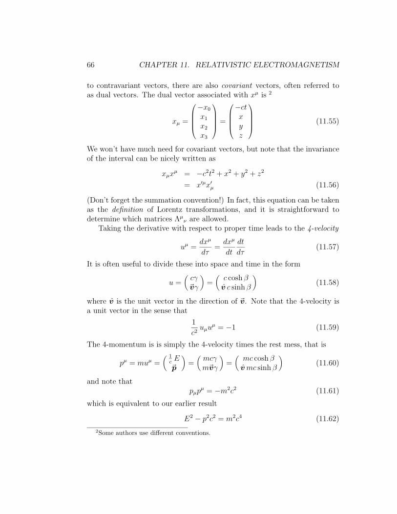
66 CHAPTER 11. RELATIVISTIC ELECTROMAGNETISM
to contravariant vectors, there are also covariant vectors, often referred toas dual vectors. The dual vector associated with xµ is 2
xµ =
−x0
x1
x2
x3
=
−ctxyz
(11.55)
We won’t have much need for covariant vectors, but note that the invarianceof the interval can be nicely written as
xµxµ = −c2t2 + x2 + y2 + z2
= x′µx′µ (11.56)
(Don’t forget the summation convention!) In fact, this equation can be takenas the definition of Lorentz transformations, and it is straightforward todetermine which matrices Λµ
ν are allowed.Taking the derivative with respect to proper time leads to the 4-velocity
uµ =dxµ
dτ=
dxµ
dt
dt
dτ(11.57)
It is often useful to divide these into space and time in the form
u =(
cγ~vγ
)
=(
c cosh βv c sinh β
)
(11.58)
where v is the unit vector in the direction of ~v. Note that the 4-velocity isa unit vector in the sense that
1
c2uµu
µ = −1 (11.59)
The 4-momentum is is simply the 4-velocity times the rest mess, that is
pµ = muµ =( 1
cE~p
)
=(
mcγm~vγ
)
=(
mc cosh βv mc sinh β
)
(11.60)
and note thatpµp
µ = −m2c2 (11.61)
which is equivalent to our earlier result
E2 − p2c2 = m2c4 (11.62)
2Some authors use different conventions.
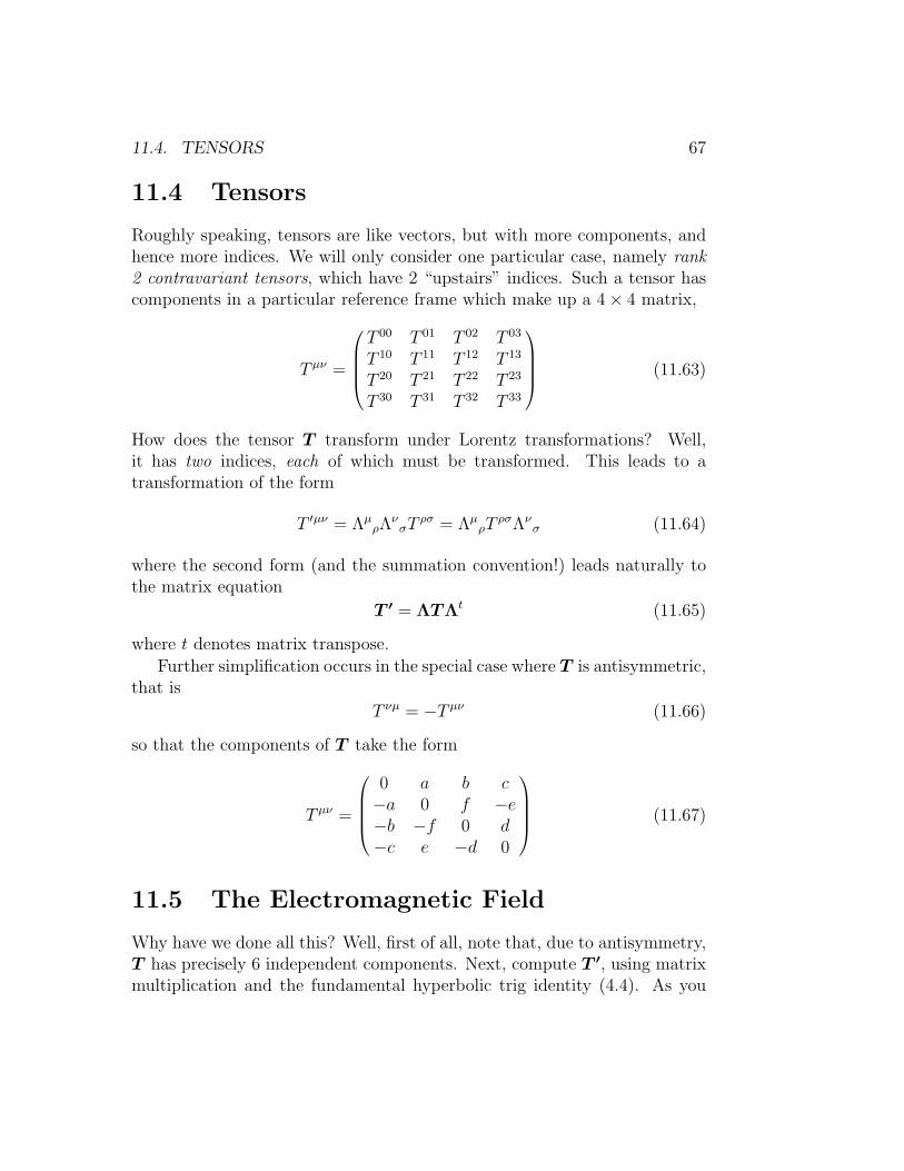
11.4. TENSORS 67
11.4 Tensors
Roughly speaking, tensors are like vectors, but with more components, andhence more indices. We will only consider one particular case, namely rank2 contravariant tensors, which have 2 “upstairs” indices. Such a tensor hascomponents in a particular reference frame which make up a 4 × 4 matrix,
T µν =
T 00 T 01 T 02 T 03
T 10 T 11 T 12 T 13
T 20 T 21 T 22 T 23
T 30 T 31 T 32 T 33
(11.63)
How does the tensor T transform under Lorentz transformations? Well,it has two indices, each of which must be transformed. This leads to atransformation of the form
T ′µν = ΛµρΛ
νσT
ρσ = ΛµρT
ρσΛνσ (11.64)
where the second form (and the summation convention!) leads naturally tothe matrix equation
T ′ = ΛTΛt (11.65)
where t denotes matrix transpose.
Further simplification occurs in the special case where T is antisymmetric,that is
T νµ = −T µν (11.66)
so that the components of T take the form
T µν =
0 a b c−a 0 f −e−b −f 0 d−c e −d 0
(11.67)
11.5 The Electromagnetic Field
Why have we done all this? Well, first of all, note that, due to antisymmetry,T has precisely 6 independent components. Next, compute T ′, using matrixmultiplication and the fundamental hyperbolic trig identity (4.4). As you
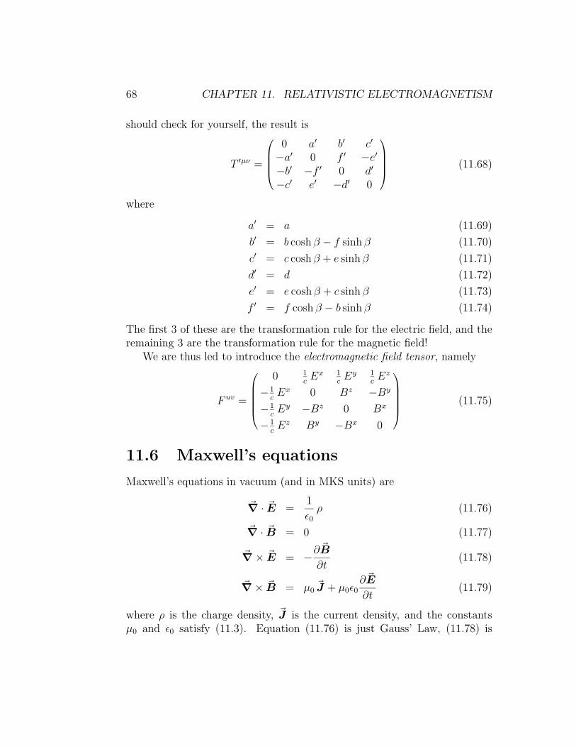
68 CHAPTER 11. RELATIVISTIC ELECTROMAGNETISM
should check for yourself, the result is
T ′µν =
0 a′ b′ c′
−a′ 0 f ′ −e′
−b′ −f ′ 0 d′
−c′ e′ −d′ 0
(11.68)
where
a′ = a (11.69)
b′ = b cosh β − f sinh β (11.70)
c′ = c cosh β + e sinh β (11.71)
d′ = d (11.72)
e′ = e cosh β + c sinh β (11.73)
f ′ = f cosh β − b sinh β (11.74)
The first 3 of these are the transformation rule for the electric field, and theremaining 3 are the transformation rule for the magnetic field!
We are thus led to introduce the electromagnetic field tensor, namely
F uv =
0 1
cEx 1
cEy 1
cEz
−1
cEx 0 Bz −By
−1
cEy −Bz 0 Bx
−1
cEz By −Bx 0
(11.75)
11.6 Maxwell’s equations
Maxwell’s equations in vacuum (and in MKS units) are
~∇ · ~E =1
ε0
ρ (11.76)
~∇ · ~B = 0 (11.77)
~∇ × ~E = −∂~B
∂t(11.78)
~∇ × ~B = µ0~J + µ0ε0
∂~E
∂t(11.79)
where ρ is the charge density, ~J is the current density, and the constantsµ0 and ε0 satisfy (11.3). Equation (11.76) is just Gauss’ Law, (11.78) is

11.6. MAXWELL’S EQUATIONS 69
Faraday’s equation, and (11.79) is Ampere’s Law corrected for the case of atime-dependent electric field. We also have the charge conservation equation
~∇ · ~J = −∂ρ
∂t(11.80)
and the Lorentz force law
~F = q(~E + ~v × ~B) (11.81)
The middle two of Maxwell equations are automatically solved by intro-ducing the scalar potential Φ and the vector potential ~A and defining
~B = ~∇ × ~A (11.82)
~E = −∂~A
∂t− ~∇Φ (11.83)
Consider the following derivatives of F :
∂F µν
∂xν=
∂F µ0
∂t+
∂F µ1
∂x+
∂F µ2
∂y+
∂F µ3
∂z(11.84)
This corresponds to four different expressions, one for each value of µ. Forµ = 0, we get
0 +1
c
∂Ex
∂x+
1
c
∂Ey
∂y+
1
c
∂Ez
∂z=
1
c~∇ · ~E =
ρ
cε0
= cµ0ρ (11.85)
where Gauss’ Law was used to get the final two equalities. Similarly, forµ = 1 we have
− 1
c2
∂Ex
∂t+ 0 +
∂Bz
∂y− ∂By
∂z(11.86)
and combining this with the expressions for µ = 2 and µ = 3 yields theleft-hand-side of
− 1
c2
∂~E
∂t+ ∇× ~B = µ0
~J (11.87)
where the right-hand-side follows from Ampere’s Law. Combining theseequations, and introducing the 4-current density
Jµ =(
cρ~J
)
(11.88)

70 CHAPTER 11. RELATIVISTIC ELECTROMAGNETISM
leads to∂F µν
∂xν= µ0
~Jµ
(11.89)
which is equivalent to the two Maxwell equations with a physical source,namely Gauss’ Law and Ampere’s Law.
Furthermore, taking the (4-dimensional!) divergence of the 4-current den-sity leads to
µ0
∂Jµ
∂xµ=
∂
∂xµ
∂F µν
∂xν= 0 (11.90)
since there is an implicit double sum over both µ and ν, and the derivativescommute but F µν is antisymmetric. (Check this by interchanging the orderof summation.) Working out the components of this equation, we have
1
c
∂J0
∂t+
∂J1
∂x+
∂J2
∂y+
∂J3
∂z= 0 (11.91)
which is just the charge conservation equation (11.80).What about the remaining equations? Introduce the dual tensor Gµν
obtained from F µν by replacing 1
c~E by ~B and ~B by −1
c~E, resulting in
Guv =
0 Bx By Bz
−Bx 0 −1
cEz 1
cEy
−By 1
cEz 0 −1
cEx
−Bz −1
cEy 1
cEx 0
(11.92)
Then the four equations∂Gµν
∂xν= 0 (11.93)
correspond to
~∇ · ~B = 0 (11.94)
−1
c
∂ ~B
∂t− 1
c~∇ × ~E = 0 (11.95)
which are precisely the two remaining Maxwell equations.Some further properties of these tensors are
1
2FµνF
µν = − 1
c2|~E|2 + |~B|2 = −1
2GµνGµν (11.96)
1
4GµνF
µν = −1
c~E · ~B (11.97)

11.6. MAXWELL’S EQUATIONS 71
where care must be taken with the signs of the components of the covarianttensors Fµν and Gµν . You may recognize these equations as correspondingto important scalar invariants of the electromagnetic field.
Finally, it is possible to solve the sourcefree Maxwell equations by intro-ducing a 4-potential
Aµ =
( 1
cΦ
~A
)
(11.98)
and defining
F µν =∂Aν
∂xµ
− ∂Aµ
∂xν
(11.99)
where again care must be taken with the signs of the components with “down-stairs” indices. Furthermore, the Lorentz force law can be rewritten in theform
m∂pµ
∂τ= quνF
µν (11.100)
Note the appearance of the proper time τ in this equation. Just as in the pre-vious chapter, this is because differentiation with respect to τ pulls througha Lorentz transformation, which makes this a valid tensor equation, valid inany inertial frame.

72 CHAPTER 11. RELATIVISTIC ELECTROMAGNETISM

Chapter 12
Problems III
12.1 Electricity vs. Magnetism I
Suppose you know that in a particular inertial frame neither the electric field~E nor the magnetic field ~B has an x component, but neither ~E nor ~B iszero. Consider another inertial frame moving with respect to the first onewith velocity v in the x-direction, and denote the electric and magnetic fieldsin this frame by ~E′ and ~B′, respectively.
1. What are the conditions on ~E and ~B, if any, and the value(s) of v, if
any, such that ~E′ vanishes for some value of v?
2. What are the conditions on ~E and ~B, if any, and the value(s) of v, if
any, such that ~B′ vanishes for some value of v?
3. What are the conditions on ~E and ~B, if any, and the value(s) of v, if
any, such that both ~E′ and ~B′ vanish for the same value of v.
4. Is it possible that ~E′ and ~B′′ vanish for different values of v?(We write ~B′′ rather than ~B′ to emphasize that ~E′ and ~B′′ are withrespect to different reference frames.)
73

74 CHAPTER 12. PROBLEMS III
1. Inserting ~E′= 0 into (11.50), we get
v = |~v| =|~E||~B|
(12.1)
since ~v is perpendicular to ~B. This is only possible if |~E| < c|~B|, which alsofollows immediately from the invariance of (11.96).
2. Inserting ~B′= 0 into (11.49), we get
v = |~v| =c2|~B||~E|
(12.2)
which is only possible if c|~B| < |~E|. This condition also follows immediatelyfrom the invariance of (11.96).3. This is not possible; if the electric and magnetic fields are both zero inany frame, they are zero in all frames.4. No; the conditions in the first two problems can not both be satisfied.
12.2 Electricity vs. Magnetism II
Suppose that in a particular inertial frame the electric field ~E and magneticfield ~B are neither perpendicular nor parallel to each other.
1. Is there another inertial frame in which the fields ~E′′
and ~B′′
are par-allel to each other?
2. Is there another inertial frame in which the fields ~E′′
and ~B′′
are per-pendicular to each other?
(You may assume without loss of generality that the inertial frames are
in relative motion parallel to the x-axis, and that neither ~B nor ~E hasan x-component. Why? Briefly justify your assumptions!)
1. Yes! Setting the cross product of (11.50) and (11.49) equal to zero, usingthe vector identity ~u× (~v × ~w) = (~u · ~w)~v − (~u ·~v)~w and the fact that ~v is
perpendicular to both ~E and ~B, leads to
~vc
1 + |~v|2
c2
=~E × c~B
|~E|2 + c2|~B|2(12.3)
2. No; ~E · ~B is invariant according to (11.97).

Chapter 13
Beyond Special Relativity
NEXT STOP: General Relativity!
13.1 Problems with Special Relativity
We began in Chapter 2 by using moving trains to model inertial referenceframes. But we made an implicit assumption beyond assuming an ideal train,with no friction and a perfectly straight track. We also assumed that therewas no gravity. Einstein’s famous thought experiment for discussing gravityis to consider a “freely falling” reference frame, typically a falling elevator.Objects thrown horizontally in such an elevator will not be seen to fall —there is no gravity (for a little while, at least!). But even here there is animplicit assumption, namely that the elevator is small compared to the Earth.
Return to our ideal train moving to the right, but now assume there isgravity. A ball thrown straight up will, according to an observer on the train,eventually turn around and fall back down, moving along a straight line, asshown in the first drawing in Figure 13.2. Since the acceleration due togravity at the surface of the Earth is taken to be constant, the exact motionis described by a quadratic equation in t. From the ground, the same effectis seen, but combined with a constant motion (linear in t) to the right. Themotion therefore takes place along a parabola; see Figure 13.1.
Now suppose that that train is also accelerating to the right with constantacceleration. Then a ball thrown straight up on the train still moves alongthe same parabolic trajectory as before (as seen from the ground), but therear wall of the train might now catch up with it before it lands! This shows,
75

76 CHAPTER 13. BEYOND SPECIAL RELATIVITY
Figure 13.1: Throwing a ball in a moving train, as seen from the ground.
first of all, that Newton’s laws fail in a noninertial frame.But let’s analyze the situation more carefully. Try to compensate by giv-
ing the ball a horizontal component of velocity. If the ball’s initial horizontalspeed is chosen appropriately, the resulting trajectory could look like the“boomerang” in the second drawing in Figure 13.2, in which (as seen fromthe train) the ball is thrown up at an angle, and returns along the same path!
What’s going here? Acceleration and gravity produce the same kind ofeffect, and what the “boomerang” is telling us is that the effective force ofgravity is no longer straight down, but rather at an angle. Throw the ballup at that angle, and it goes “up” and “down” in a straight line!
13.2 Tidal Effects
Consider now two objects falling towards the Earth, but far from it, as shownin the first sketch in Figure 13.3. Both objects fall towards the center of theEarth — which is not quite the same direction for each object. Assuming theobjects start at the same distance from the Earth, their paths will converge.
Figure 13.2: Throwing a ball in a moving train, as seen from the train.

13.3. DIFFERENTIAL GEOMETRY 77
Figure 13.3: Two objects falling towards the Earth from far away either movecloser together or further apart depending on their initial configuration.
Now, if they don’t realize they are falling — by virtue of being in a largefalling elevator, say — they will nevertheless notice that they are approachingeach other. This is gravity!
Similarly, if, as shown in the second sketch, one object starts out abovethe other, it is slightly further from the Earth, and hence experiences aslightly weaker gravitational attraction. Thus, the lower object will alwaysaccelerate more then the upper one, and so the distance between the objectswill increase.
This effect causes tides! To see this, imagine that the Earth is fallingtowards the Moon, as shown in Figure 13.4. The motion of the center of theEarth is not relevant; subtract it out. What is left is a relative attraction atboth the nearest and furthest points from the Moon, and a relative repulsionon either side. This explains why there are two, not one, high (and low) tidesevery day! A similar effect, but roughly half as strong, is caused by the Sun.
13.3 Differential Geometry
In 2-dimensions, Euclidean geometry is the geometry of a flat piece of paper.But there are also of course curved 2-dimensional surfaces. The simplest ofthese is the sphere, which has constant positive curvature and is a model of(double) elliptic geometry. Another important example is the hyperboloid,which also has constant curvature, and is a model of hyperbolic geometry.Hyperbolic and elliptic geometry form the 2 main categories of non-Euclidean

78 CHAPTER 13. BEYOND SPECIAL RELATIVITY
Figure 13.4: Tides are caused by the Earth falling towards the Moon!
geometries.
In fact, any 2-dimensional surface in Euclidean 3-space provides a possiblegeometry, most of which are curved. However, it is important to realizethat distances are always positive in all such geometries. One measures thedistance between 2 points on such a surface by stretching a string betweenthem along the surface. This does not measure the (3-dimensional) Euclideandistance between the points, but instead corresponds to integrating the arc-length along the shortest path between them.
In hyperbola geometry, we instead made a fundamental change to thedistance function, allowing it to become negative or zero. If there is preciselyone (basis) direction in which distances turn out to be negative, such ge-ometries are said to have Lorentzian signature, as opposed to the Euclideansignature of ordinary surfaces. As implied by the way we have drawn it,hyperbola geometry turns out to be flat in a well-defined sense, which im-mediately raises the question of whether there are curved geometries withLorentzian signature.
The mathematical study of curved surfaces forms a central part of dif-ferential geometry, and the further restriction to surfaces on which distancesare positive is known as Riemannian geometry. The much harder case ofLorentzian signature is known, not surprisingly, as Lorentzian geometry, andthe important special case where the curvature vanishes is Minkowskian ge-ometry. This classification of geometries by signature and curvature is sum-marized in Table 13.5.
What does this have to do with physics? We have seen that hyperbola

13.4. GENERAL RELATIVITY 79
signature flat curved
(+ + ... +) Euclidean Riemannian(− + ... +) Minkowskian Lorentzian
Table 13.5: Classification of geometries.
geometry, more correctly called Minkowski space, is the geometry of specialrelativity. Lorentzian geometry turns out to be the geometry of generalrelativity. In short, according to Einstein, gravity is curvature!
13.4 General Relativity
Just as one studies flat (2-dimensional) Euclidean geometry before studyingcurved surfaces, one studies special relativity before general relativity. Butthe analogy goes much further.
The basic notion in Euclidean geometry is the distance between twopoints, which is given by the Pythagorean theorem. The basic notion ona curved surface is still the distance “function”, but this is now an statementabout infinitesimal distances. Euclidean geometry is characterized by theline element
ds2 = dx2 + dy2 (13.1)
which can be used to find the distance along any curve. The simplest curvedsurface, a sphere of radius r, can be characterized by the line element
ds2 = r2 dθ2 + r2 sin2 θ dφ2 (13.2)
Remarkably, it is possible to calculate the curvature of the sphere from thisline element alone; it is not necessary to use any 3-dimensional geometry.It’s also possible to calculate the “straight lines”, that is, the shortest pathbetween two given points. These are, of course, straight lines in the plane,but great circles (diameters) on the sphere.
Similarly, special relativity is characterized by the line element 1
ds2 = −dt2 + dx2 (13.3)
1Note that we have set c = 1!

80 CHAPTER 13. BEYOND SPECIAL RELATIVITY
which is every bit as flat as a piece of paper. You get general relativity simplyby considering more general line elements!
Of course, it’s not quite that simple. The line element must have a minussign. And the curvature must correspond to a physical source of gravity —that’s where Einstein’s field equations come in. But, given a line element,one can again calculate the “straight lines”, which now correspond to freelyfalling observers! Matter curves the universe, and the curvature tells objectswhich paths are “straight” — that’s gravity!
Here are two examples to whet your appetite further.The (3-dimensional) line element
ds2 = −dt2 + sin2(t)(
dθ2 + sin2 θ dφ2)
(13.4)
describes the 2-dimensional surface of a spherical balloon, whose radiuschanges with time. This roughly corresponds to a cosmological model foran expanding universe produced by a Big Bang. By studying the propertiesof this model more carefully, you will be led to ask good questions aboutrelativistic cosmology.
And finally, the line element
ds2 = −(
1 − 2m
r
)
dt2 +dr2
1 − 2m
r
(13.5)
describes a simplified model of a black hole, with an apparent singularity atr = 2m, which however is just due to a poor choice of coordinates. Tryingto understand what actually happens at r = 2m will give you some under-standing of what a black hole really is.
If you wish to pursue these ideas further, you may wish to take a lookat an introductory textbook on general relativity, such as d’Inverno [5] orTaylor & Wheeler [6].

Bibliography
[1] Edwin F. Taylor and John Archibald Wheeler, Spacetime Physics,W. H. Freeman, San Francisco, 1963.
[2] Edwin F. Taylor and John Archibald Wheeler, Spacetime Physics,second edition, W. H. Freeman, New York, 1992.
[3] David J. Griffiths, Introduction to Electrodynamics, 3rd edition,Prentice Hall, Upper Saddle River, 1999.
[4] Tevian Dray, The Twin Paradox Revisited, Am. J. Phys. 58, 822–825(1990).
[5] Ray A. d’Inverno, Introducing Einstein’s Relativity, Oxford Uni-versity Press, Oxford, 1992.
[6] Edwin F. Taylor, John Archibald Wheeler, Exploring Black Holes:
Introduction to General Relativity, Addison-Wesley, San Francisco,2000.
81