geometry of trace spaces - laboratoire paul...
TRANSCRIPT

Geometry of Trace Spaces
Eric Goubault
CEA LIST and Ecole Polytechnique, France
joint work with Samuel Mimram, Emmanuel Haucourt, Christine Tasson, LisbethFajstrup, Martin Raussen
Inaugural Conference Labex CEMPI
27th of September 2012
E. Goubault
Contents of the talk
A rush tour of static analysis, and of geometric semantics ofconcurrent programs
Combinatorics/algorithmics of trace spaces
Very quick application to static analysis of programs
E. Goubault

Typical static analysis
Given a program, how to prove some form of correctness?(executions won’t do)
Generally: (a) to compute invariants, i.e. properties which holdtrue on any execution(b) to compute liveness properties, i.e. properties that willeventually be true (will terminate, will deadlock etc.)
Classical steps:
(1) interleaving semantics, collecting semantics for (a) (only)
(2) abstraction (Galois connections etc.)
(3) computation of least fixpoints - resolution of large systems ofequations
We are looking for a more efficient step (1) ((2) and (3) for someother talk!)
E. Goubault
Use of invariants
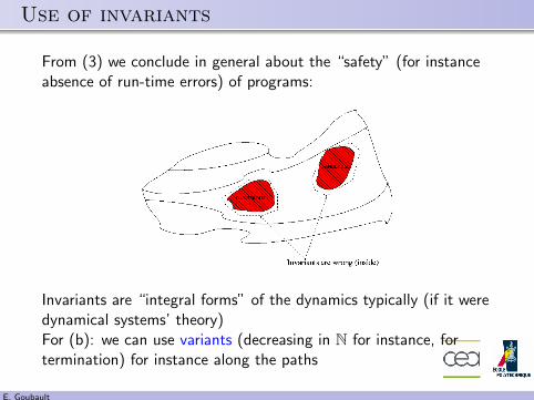
From (3) we conclude in general about the “safety” (for instanceabsence of run-time errors) of programs:
Invariants are “integral forms” of the dynamics typically (if it weredynamical systems’ theory)For (b): we can use variants (decreasing in N for instance, fortermination) for instance along the paths
E. Goubault
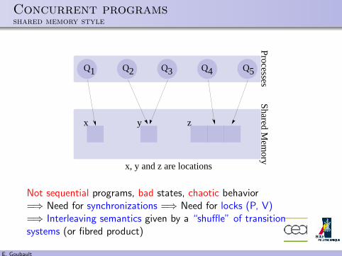
Concurrent programsshared memory style
2Q1Q 3Q 4Q 5QShared M
emory
Processes
x y z
x, y and z are locations
Not sequential programs, bad states, chaotic behavior=⇒ Need for synchronizations =⇒ Need for locks (P, V)=⇒ Interleaving semantics given by a “shuffle” of transitionsystems (or fibred product)
E. Goubault
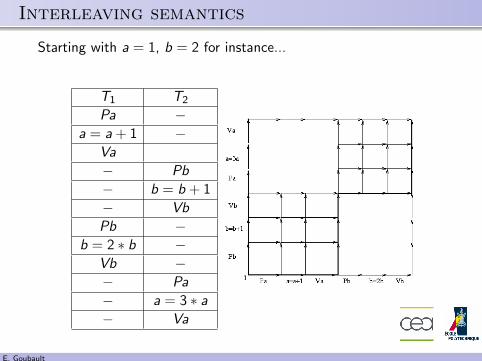
Interleaving semantics
Starting with a = 1, b = 2 for instance...
T1 T2
Pa −a = a + 1 −
Va
− Pb
− b = b + 1
− Vb
Pb −b = 2 ∗ b −
Vb −− Pa
− a = 3 ∗ a
− Va
E. Goubault
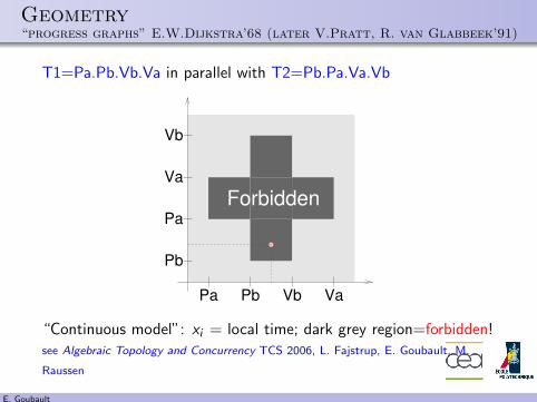
Geometry“progress graphs” E.W.Dijkstra’68 (later V.Pratt, R. van Glabbeek’91)
T1=Pa.Pb.Vb.Va in parallel with T2=Pb.Pa.Va.Vb
Pa Pb Vb Va
Pb
Pa
Va
Vb
Forbidden
“Continuous model”: xi = local time; dark grey region=forbidden!see Algebraic Topology and Concurrency TCS 2006, L. Fajstrup, E. Goubault, M.
Raussen
E. Goubault
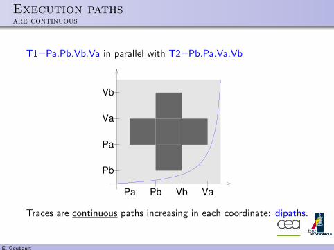
Execution pathsare continuous
T1=Pa.Pb.Vb.Va in parallel with T2=Pb.Pa.Va.Vb
Pa Pb Vb Va
Pb
Pa
Va
Vb
Traces are continuous paths increasing in each coordinate: dipaths.
E. Goubault
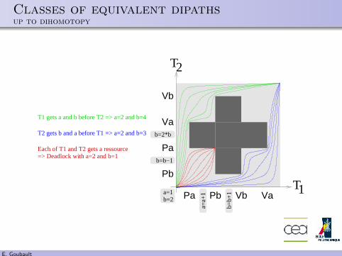
Classes of equivalent dipathsup to dihomotopy
Pa Pb Vb Va
Pb
Pa
Va
Vb
T2
T1
b=2*b
b=b−1
a=a+
1
b=b+
1
b=2a=1
T1 gets a and b before T2 => a=2 and b=4
T2 gets b and a before T1 => a=2 and b=3
Each of T1 and T2 gets a ressource=> Deadlock with a=2 and b=1
E. Goubault
Goal
When verifying a concurrent program,there is a priori a large number of possible interleavings to check
(exponential in the number of processes)
Many executions are equivalent:we want here to provide a minimal number of execution traces
which describe all the possible cases
E. Goubault
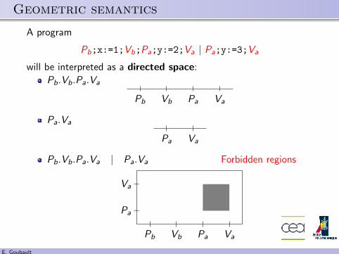
Geometric semantics
A program
Pb;x:=1;Vb;Pa;y:=2;Va | Pa;y:=3;Va
will be interpreted as a directed space:
Pb.Vb.Pa.Va
Pb Vb Pa Va
Pa.Va
Pa Va
Pb.Vb.Pa.Va | Pa.Va Forbidden regions
Pb Vb Pa Va
Pa
Va
E. Goubault
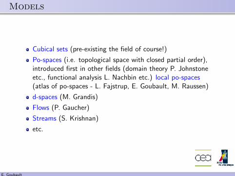
Models
Cubical sets (pre-existing the field of course!)
Po-spaces (i.e. topological space with closed partial order),introduced first in other fields (domain theory P. Johnstoneetc., functional analysis L. Nachbin etc.) local po-spaces(atlas of po-spaces - L. Fajstrup, E. Goubault, M. Raussen)
d-spaces (M. Grandis)
Flows (P. Gaucher)
Streams (S. Krishnan)
etc.
E. Goubault
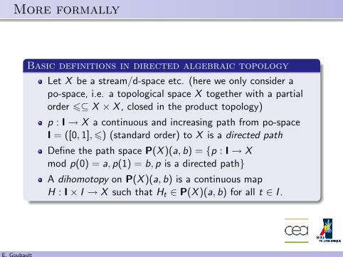
More formally
Basic definitions in directed algebraic topology
Let X be a stream/d-space etc. (here we only consider apo-space, i.e. a topological space X together with a partialorder 6⊆ X × X , closed in the product topology)
p : I→ X a continuous and increasing path from po-spaceI = ([0, 1],6) (standard order) to X is a directed path
Define the path space P(X )(a, b) = {p : I→ Xmod p(0) = a, p(1) = b, p is a directed path}A dihomotopy on P(X )(a, b) is a continuous mapH : I× I → X such that Ht ∈ P(X )(a, b) for all t ∈ I .
E. Goubault
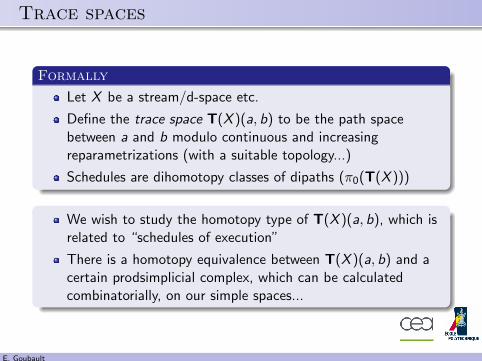
Trace spaces
Formally
Let X be a stream/d-space etc.
Define the trace space T(X )(a, b) to be the path spacebetween a and b modulo continuous and increasingreparametrizations (with a suitable topology...)
Schedules are dihomotopy classes of dipaths (π0(T(X )))
We wish to study the homotopy type of T(X )(a, b), which isrelated to “schedules of execution”
There is a homotopy equivalence between T(X )(a, b) and acertain prodsimplicial complex, which can be calculatedcombinatorially, on our simple spaces...
E. Goubault
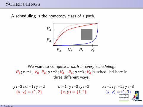
Schedulings
A scheduling is the homotopy class of a path.
Pb Vb Pa Va
Pa
Va
We want to compute a path in every scheduling.Pb;x:=1;Vb;Pa;y:=2;Va | Pa;y:=3;Va is scheduled here in
three different ways:
y:=3;x:=1;y:=2 x:=1;y:=3;y:=2 x:=1;y:=2;y:=3(x , y) = (1, 2) (x , y) = (1, 2) (x , y) = (1, 3)
E. Goubault
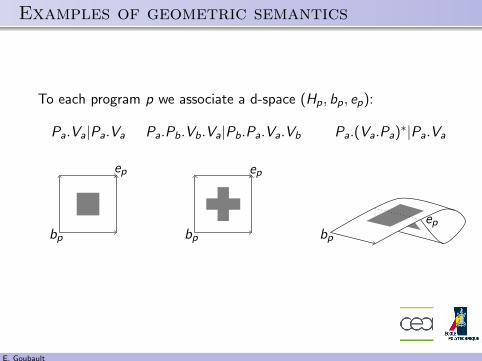
Examples of geometric semantics
To each program p we associate a d-space (Hp, bp, ep):
Pa.Va|Pa.Va Pa.Pb.Vb.Va|Pb.Pa.Va.Vb Pa.(Va.Pa)∗|Pa.Va
bp
ep
bp
ep
bp
ep
E. Goubault
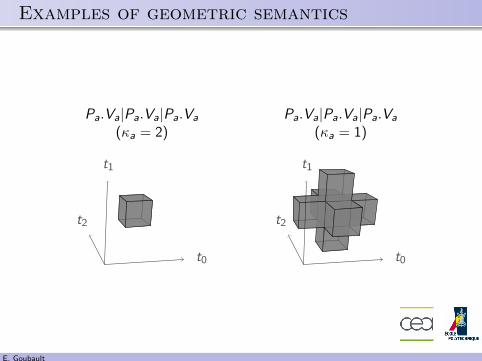
Examples of geometric semantics
Pa.Va|Pa.Va|Pa.Va Pa.Va|Pa.Va|Pa.Va
(κa = 2) (κa = 1)
t0
t1
t2
t0
t1
t2
E. Goubault
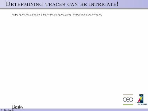
Determining traces can be intricate!
Px.Py.Pz.Vx.Pw.Vz.Vy.Vw | Pu.Pv.Px.Vu.Pz.Vv.Vx.Vz Py.Pw.Vy.Pu.Vw.Pv.Vu.Vv
LipskyE. Goubault
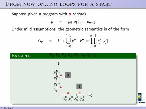
From now on...no loops for a start
Suppose given a program with n threads
p = p0|p1| . . . |pn−1
Under mild assumptions, the geometric semantics is of the form
Gp = ~I n \l−1⋃i=0
R i ; R i =n−1∏j=0
]x ij , y
ij [
Example Pa.Va.Pb.Vb|Pb.Vb.Pa.Va
t0
t1
0
1
x00 y0
0 x10 y1
0
x11
y11
x01
y01
a b
b
a
E. Goubault

Determining trace spaces
The trace space between two points b and e is the space ofdirected paths modulo reparameterization, suitably topologized...
To determine it (its connected components?), the main (naive?)idea is to extend the forbidden cubes downwards in variousdirections and look whether there is a path from b to e.
t0
t1
t0
t1
t0
t1
By combining those information, we will be able to compute tracesmodulo homotopy.
The directions in which to extend the holes will be coded byboolean matrices M.
E. Goubault
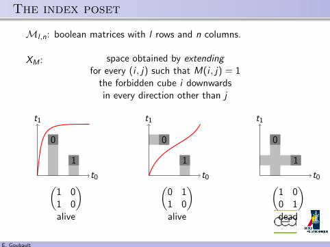
The index poset
Ml ,n: boolean matrices with l rows and n columns.
XM : space obtained by extendingfor every (i , j) such that M(i , j) = 1
the forbidden cube i downwardsin every direction other than j
0
1
t0
t1
0
1
t0
t1
0
1
t0
t1
(1 01 0
) (0 11 0
) (1 00 1
)alive alive dead
E. Goubault
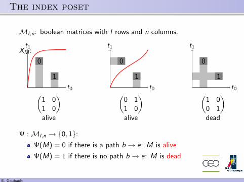
The index poset
Ml ,n: boolean matrices with l rows and n columns.
XM :
0
1
t0
t1
0
1
t0
t1
0
1
t0
t1
(1 01 0
) (0 11 0
) (1 00 1
)alive alive dead
Ψ :Ml ,n → {0, 1}:Ψ(M) = 0 if there is a path b → e: M is alive
Ψ(M) = 1 if there is no path b → e: M is dead
E. Goubault
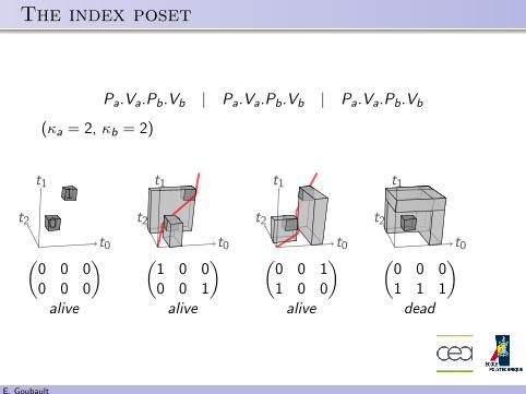
The index poset
Pa.Va.Pb.Vb | Pa.Va.Pb.Vb | Pa.Va.Pb.Vb
(κa = 2, κb = 2)
0
1
t0
t1
t2
t0
t1
t2
t0
t1
t2
t0
t1
t2
(0 0 00 0 0
) (1 0 00 0 1
) (0 0 11 0 0
) (0 0 01 1 1
)alive alive alive dead
E. Goubault

The index poset
Alive and dead?
Important matrices are
the dead poset D(X ) = {M ∈MCl ,n / Ψ(M) = 1}.
the index poset C(X ) = {M ∈MRl ,n / Ψ(M) = 0} (the alive
matrices).
consider the entrywise ordering (0 < 1) on matrices.
General results:
D(X ) C(X ) trace spaces, up to homotopy equivalence
(hence at least homotopy classes of traces...)
E. Goubault
The dead poset
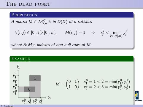
Proposition
A matrix M ∈MCl ,n is in D(X ) iff it satisfies
∀(i , j) ∈ [0 : l [×[0 : n[, M(i , j) = 1 ⇒ x ij < min
i ′∈R(M)y i ′j
where R(M): indexes of non-null rows of M.
Example
t0
t1
0
1
x00 x1
0 y00 y1
0
x01
y01
x11
y11
M =
(0 11 0
)x01 = 1 < 2 = min(y0
1 , y11 )
x10 = 2 < 3 = min(y0
0 , y10 )
E. Goubault
The index poset
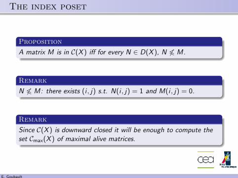
Proposition
A matrix M is in C(X ) iff for every N ∈ D(X ), N 66 M.
Remark
N 66 M: there exists (i , j) s.t. N(i , j) = 1 and M(i , j) = 0.
Remark
Since C(X ) is downward closed it will be enough to compute theset Cmax(X ) of maximal alive matrices.
E. Goubault
Connected components
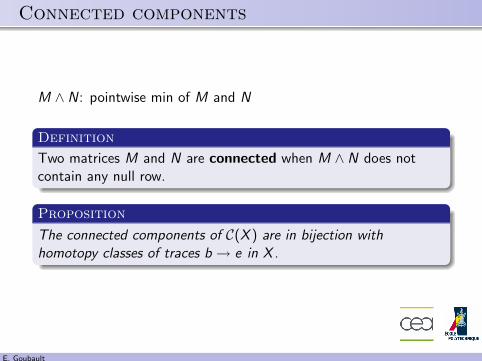
M ∧ N: pointwise min of M and N
Definition
Two matrices M and N are connected when M ∧ N does notcontain any null row.
Proposition
The connected components of C(X ) are in bijection withhomotopy classes of traces b → e in X .
E. Goubault
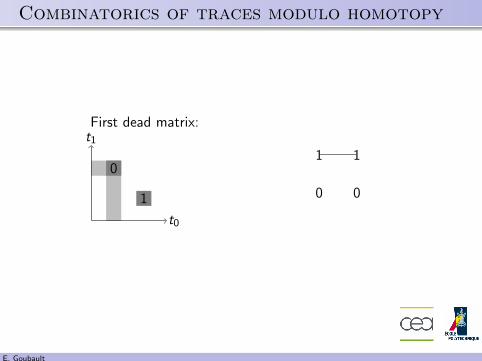
Combinatorics of traces modulo homotopy
First dead matrix:
0
1
t0
t11 1
0 0
E. Goubault

Combinatorics of traces modulo homotopy
Second dead matrix:
0
1
t0
t10 0
1 1
E. Goubault
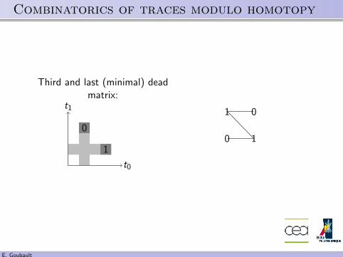
Combinatorics of traces modulo homotopy
Third and last (minimal) deadmatrix:
0
1
t0
t1 1 0
0 1
E. Goubault
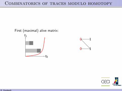
Combinatorics of traces modulo homotopy
First (maximal) alive matrix:
t0
t10 1
0 1
E. Goubault

Combinatorics of traces modulo homotopy
Second alive matrix:
t0
t11 0
1 0
E. Goubault
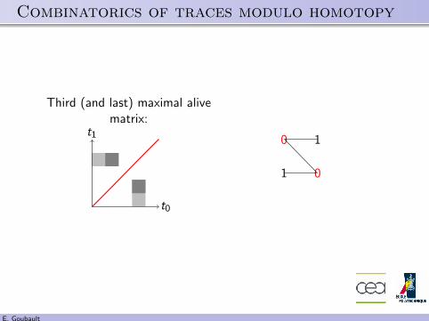
Combinatorics of traces modulo homotopy
Third (and last) maximal alivematrix:
t0
t1 0 1
1 0
E. Goubault
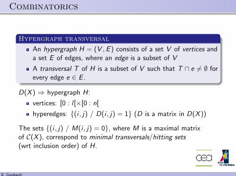
Combinatorics
Hypergraph transversal
An hypergraph H = (V ,E ) consists of a set V of vertices anda set E of edges, where an edge is a subset of V
A transversal T of H is a subset of V such that T ∩ e 6= ∅ forevery edge e ∈ E .
D(X ) ⇒ hypergraph H:
vertices: [0 : l [×[0 : n[
hyperedges: {(i , j) / D(i , j) = 1} (D is a matrix in D(X ))
The sets {(i , j) / M(i , j) = 0}, where M is a maximal matrixof C(X ), correspond to minimal transversals/hitting sets(wrt inclusion order) of H.
E. Goubault
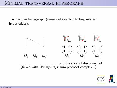
Minimal transversal hypergraph
...is itself an hypergraph (same vertices, but hitting sets ashyper-edges):
. .
.
M2
.
M3 M1
t0
t1
t0
t1
t0
t1
(1 01 0
) (0 10 1
) (0 11 0
)M1 M2 M3
and they are all disconnected.(linked with Herlihy/Rajsbaum protocol complex...)
E. Goubault
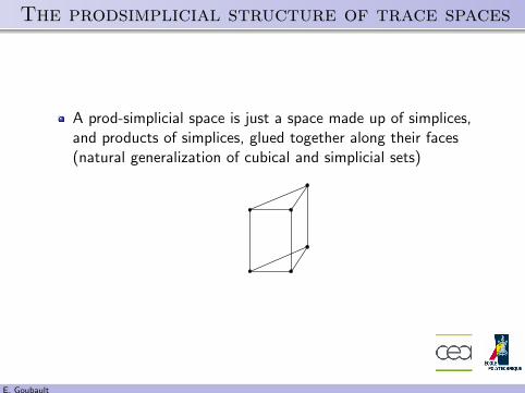
The prodsimplicial structure of trace spaces
A prod-simplicial space is just a space made up of simplices,and products of simplices, glued together along their faces(natural generalization of cubical and simplicial sets)
E. Goubault

The prodsimplicial structure of trace spaces
A prod-simplicial space is just a space made up of simplices,and products of simplices, glued together along their faces(natural generalization of cubical and simplicial sets)
Example:
E. Goubault
The prodsimplicial structure of trace spaces
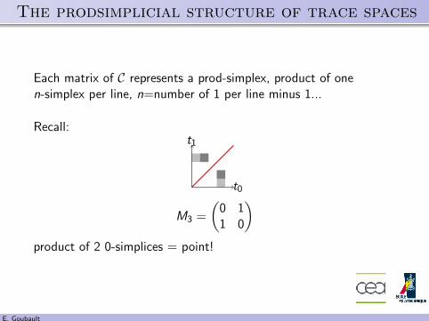
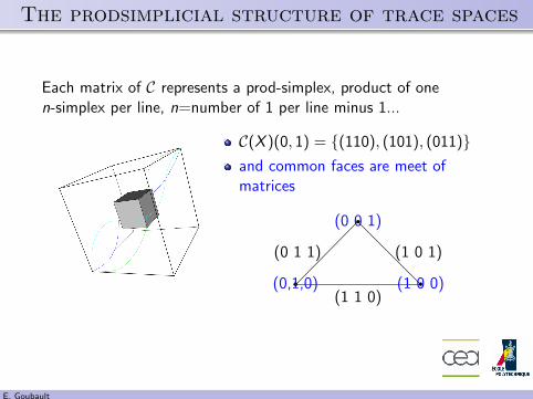
Each matrix of C represents a prod-simplex, product of onen-simplex per line, n=number of 1 per line minus 1...
Recall:
t0
t1
M3 =
(0 11 0
)product of 2 0-simplices = point!
E. Goubault
The prodsimplicial structure of trace spaces
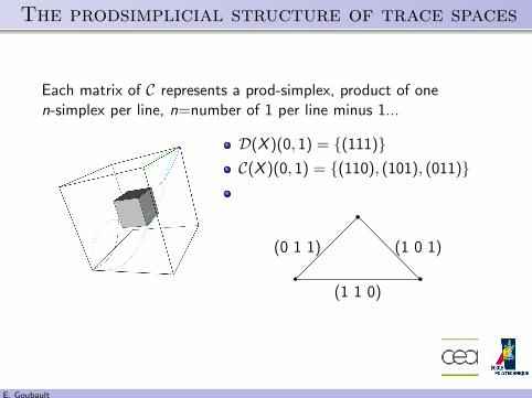
Each matrix of C represents a prod-simplex, product of onen-simplex per line, n=number of 1 per line minus 1...
D(X )(0, 1) = {(111)}C(X )(0, 1) = {(110), (101), (011)}
(1 1 0)
(1 0 1)(0 1 1)
E. Goubault
The prodsimplicial structure of trace spaces
Each matrix of C represents a prod-simplex, product of onen-simplex per line, n=number of 1 per line minus 1...
C(X )(0, 1) = {(110), (101), (011)}and common faces are meet ofmatrices
(0,1,0)(1 1 0)
(1 0 0)
(1 0 1)
(0 0 1)
(0 1 1)
E. Goubault
The prodsimplicial structure of trace spaces
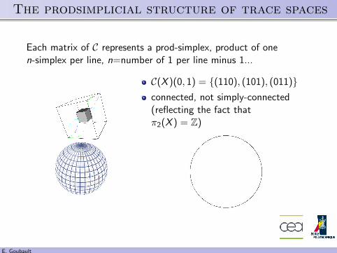
Each matrix of C represents a prod-simplex, product of onen-simplex per line, n=number of 1 per line minus 1...
C(X )(0, 1) = {(110), (101), (011)}connected, not simply-connected(reflecting the fact thatπ2(X ) = Z)
E. Goubault
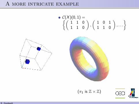
A more intricate example
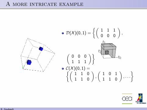
D(X )(0, 1) =
{(1 1 10 0 0
),
(0 0 01 1 1
)}t0
t1
t2
C(X )(0, 1) ={(1 1 01 1 0
),
(1 0 11 1 0
), . . .
}
E. Goubault
A more intricate example
C(X )(0, 1) ={(1 1 01 1 0
),
(1 0 11 1 0
), . . .
}
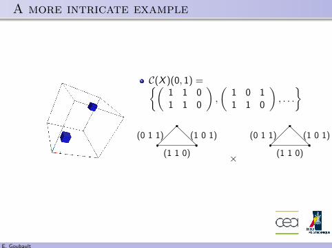
(1 1 0)
(1 0 1)(0 1 1)
× (1 1 0)
(1 0 1)(0 1 1)
E. Goubault
A more intricate example
C(X )(0, 1) ={(1 1 01 1 0
),
(1 0 11 1 0
), . . .
}
(π1 is Z× Z)
E. Goubault
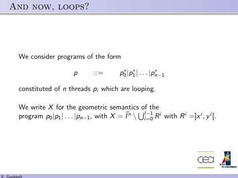
And now, loops?
We consider programs of the form
p ::= p∗0 |p∗1 | . . . |p∗n−1
constituted of n threads pi which are looping.
We write X for the geometric semantics of theprogram p0|p1| . . . |pn−1, with X = ~I n \
⋃l−1i=0 R i with R i =]x i , y i [.
E. Goubault
Delooping
This is a particular case of delooping (here, just deloop once inevery direction)
Given a n-dimensional vector m whose components (mj)06j<n arein N, we write pm for the m-delooping of p, i.e. the program
pm00 |p
m11 | . . . |p
mn−1
n−1
and X m for the associated geometric semantics.
The trace space (at least its connected components) of all X m canbe generated fairly easily given what we did before...
E. Goubault
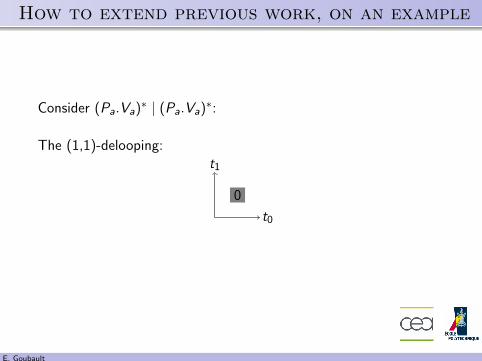
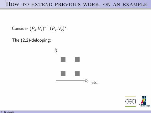
How to extend previous work, on an example
Consider (Pa.Va)∗ | (Pa.Va)∗:
The (1,1)-delooping:
0
t0
t1
E. Goubault
How to extend previous work, on an example
Consider (Pa.Va)∗ | (Pa.Va)∗:
The (2,2)-delooping:
t0
t1
etc.
E. Goubault
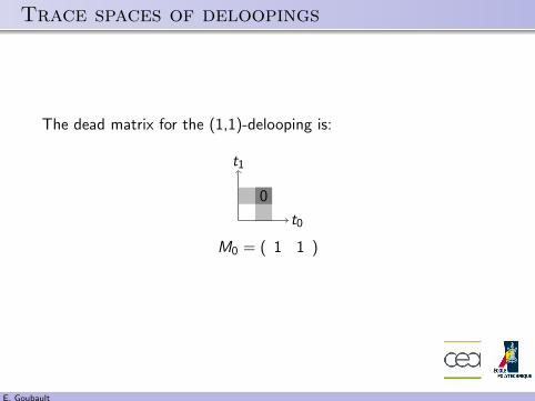
Trace spaces of deloopings
The dead matrix for the (1,1)-delooping is:
0
t0
t1
M0 = ( 1 1 )
E. Goubault
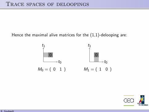
Trace spaces of deloopings
Hence the maximal alive matrices for the (1,1)-delooping are:
0
t0
t1
0
t0
t1
M0 = ( 0 1 ) M1 = ( 1 0 )
E. Goubault
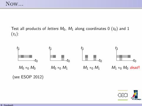
Now...
Test all products of letters M0, M1 along coordinates 0 (t0) and 1(t1):
t0
t1
M0 ∗0 M0
t0
t1
M0 ∗0 M1
t0
t1
M1 ∗0 M1
t0
t1
M1 ∗0 M0 dead!
(see ESOP 2012)
E. Goubault
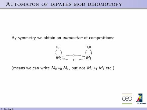
Automaton of dipaths mod dihomotopy
By symmetry we obtain an automaton of compositions:
M0
0,1
��0 ++
M11kk
1,0
��
(means we can write M0 ∗0 M1, but not M0 ∗1 M1 etc.)
E. Goubault

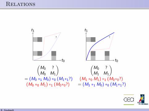
Relations!
We may have extra relations among the words in this automaton!Consider all possible concatenations of 2 letters on t0 and on t1:
?
t0
t1?
t0
t1?
t0
t1?
t0
t1
(M0 ?M0 M0
) (M0 ?M0 M1
) (M0 ?M1 M1
) (M1 ?M1 M1
)(M0 ∗0 M0) ∗1 (M0∗0?) (M0 ∗0 M1) ∗1 (M0∗0?) (M1 ∗0 M1) ∗1 (M0∗0?) (M1 ∗0 M1) ∗1 (M1∗0?)
Only the two in the middle give rise to commutations.
E. Goubault
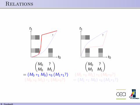
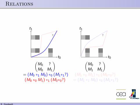
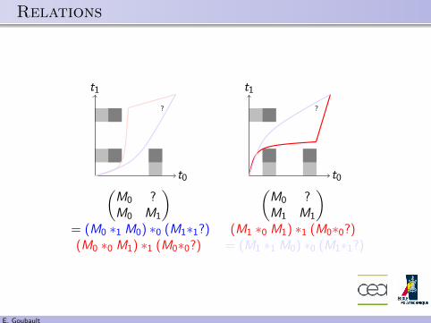
Relations
?
t0
t1
?
t0
t1
(M0 ?M0 M1
) (M0 ?M1 M1
)= (M0 ∗1 M0) ∗0 (M1∗1?) (M1 ∗0 M1) ∗1 (M0∗0?)(M0 ∗0 M1) ∗1 (M0∗0?) = (M1 ∗1 M0) ∗0 (M1∗1?)
E. Goubault
Relations
?
t0
t1
?
t0
t1
(M0 ?M0 M1
) (M0 ?M1 M1
)= (M0 ∗1 M0) ∗0 (M1∗1?) (M1 ∗0 M1) ∗1 (M0∗0?)(M0 ∗0 M1) ∗1 (M0∗0?) = (M1 ∗1 M0) ∗0 (M1∗1?)
E. Goubault
Relations
?
t0
t1
?
t0
t1
(M0 ?M0 M1
) (M0 ?M1 M1
)= (M0 ∗1 M0) ∗0 (M1∗1?) (M1 ∗0 M1) ∗1 (M0∗0?)(M0 ∗0 M1) ∗1 (M0∗0?) = (M1 ∗1 M0) ∗0 (M1∗1?)
E. Goubault
Relations
?
t0
t1
?
t0
t1
(M0 ?M0 M1
) (M0 ?M1 M1
)= (M0 ∗1 M0) ∗0 (M1∗1?) (M1 ∗0 M1) ∗1 (M0∗0?)(M0 ∗0 M1) ∗1 (M0∗0?) = (M1 ∗1 M0) ∗0 (M1∗1?)
E. Goubault
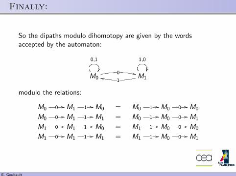
Finally:
So the dipaths modulo dihomotopy are given by the wordsaccepted by the automaton:
M0
0,1
��0 ++
M11kk
1,0
��
modulo the relations:
M0 0 // M1 1 // M0 = M0 1 // M0 0 // M0
M0 0 // M1 1 // M1 = M0 1 // M0 0 // M1
M1 0 // M1 1 // M0 = M1 1 // M0 0 // M0
M1 0 // M1 1 // M1 = M1 1 // M0 0 // M1
E. Goubault

Application to static analysis
Suppose we want to analyze program
(Pa.a = a− 1.Va)∗ | (Pa.a = a/2.Va)∗
What are the possible sets of values reached, for a, starting witha ∈ [0, 1]?
Write (A0: set of possible values for a at the end of dipath M0, A1:set of possible values for a at the end of dipath M1):
M0 : [a← a− 1]
0,1
��0 ..
M1 : [a← a2 ]
1nn
1,0
{A0 ∪ = A0 − 1 ∪ A1
A1 ∪ = A12 ∪ A0
(plus relations) as some form of CFG for our program...theninterpret this as a least-fixed point equations over the lattice ofintervals...
Finds invariant a∞ =]−∞, 1]
E. Goubault
Conclusion and future work
Lots of experiments (implementation in “ALCOOL”) and lotsof mathematics to be investigated yet on trace spaces...
Applications: possibility/impossibility results for fault-tolerantprotocols (a la Herlihy/Rajsbaum)
Extension to randomized algorithms: random simplicial sets!Application: possibility of consensus...
Logical interpretation?
E. Goubault
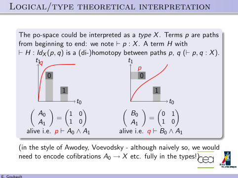
Logical/type theoretical interpretation
The po-space could be interpreted as a type X . Terms p are pathsfrom beginning to end: we note ` p : X . A term H with` H : IdX (p, q) is a (di-)homotopy between paths p, q (` p, q : X ).
0
1
q
t0
t1
0
1
p
t0
t1
(A0
A1
)=
(1 01 0
) (B0
A1
)=
(0 11 0
)alive i.e. p ` A0 ∧ A1 alive i.e. q ` B0 ∧ A1
(in the style of Awodey, Voevodsky - although naively so, we wouldneed to encode cofibrations A0 → X etc. fully in the types!)
E. Goubault
Thanks for your attention!
http://acat.lix.polytechnique.frhttp://www.appliedtopology.org/
http://labex-digicosme.fr/
E. Goubault