geometry subsystem design
TRANSCRIPT
Geometry Subsystem Design
Lan-Da Van (范倫達), Ph. D.
Department of Computer Science
National Chiao Tung University Hisnchu, Taiwan
Fall, 2018
2018/9/101

Outline
• Geometry Subsystem
• Introduction to Shading Algorithms
• Proposed Low-Complexity Subdivision Algorithm
• Proposed Power-Area Efficient Geometry Engine
• Implementation and Comparison Results
• Summary
2
Geometry Subsystem
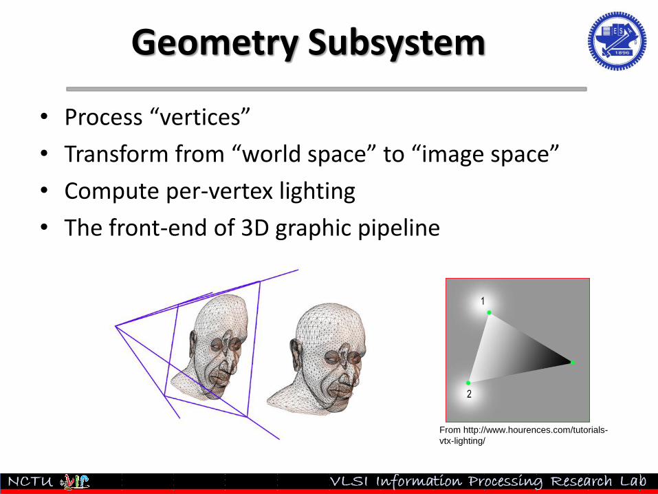
• Process “vertices”
• Transform from “world space” to “image space”
• Compute per-vertex lighting
• The front-end of 3D graphic pipeline
3From http://www.hourences.com/tutorials-
vtx-lighting/

Geometry Subsystem
4
3D Graphics System
Source: B.-S. Liang, Y.-C. Lee, W.-C. Yeh, C.-W. Jen, "Index rendering: hardware-efficient architecture
for 3-D graphics in multimedia system," IEEE Trans. Multimedia, vol. 4, no. 3, pp. 343-360, Sep. 2002.

VLSI Signal Processing System Design Spectrum
System Level
Algorithm Level
Architecture Level
Circuit Level
Logic Level
Process Level

Introduction to Shading Algorithms
• Gouraud shading
– Per-vertex lighting
– Less computation requirement
– Not good shading quality
• Phong shading
– Per-pixel lighting
– Huge computation requirement
– Smooth and more realistic highlight
6
Introduction to Shading Algorithms
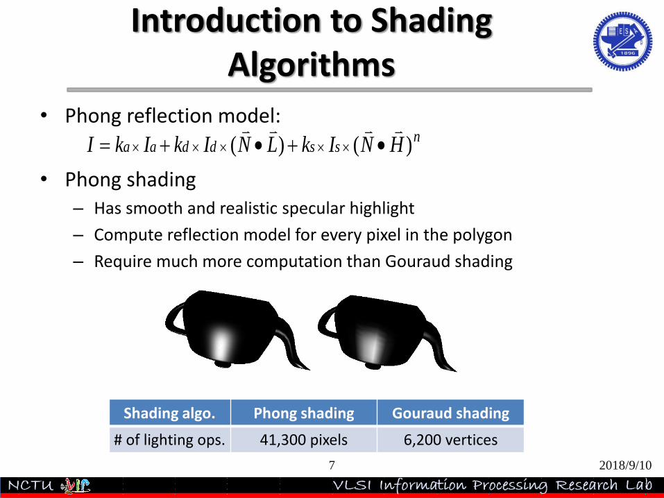
• Phong reflection model:
• Phong shading– Has smooth and realistic specular highlight
– Compute reflection model for every pixel in the polygon
– Require much more computation than Gouraud shading
2018/9/107
nssddaa HNIkLNIkIkI )()(
Shading algo. Phong shading Gouraud shading
# of lighting ops. 41,300 pixels 6,200 vertices

Introduction to Shading Algorithms
• Existing Approximate Phong Shading Algorithms– Taylor expansion based approximate algorithms
– Spherical interpolation based approximate algorithms
– Mixed shading
– Subdivision based approximate algorithms
8
Mixed shading Subdivision
No pass
Pass

Motivation
• Smooth highlight and Phong shading quality with low power consumption is desired.– Gouraud shading possesses lower power consumption but poor
quality.
– Phong shading possesses high quality but consumes more power.
– Until now, no one explores the architecture of subdivision algorithms
• A low complexity subdivision algorithm is proposed for lower power-area and near-Phong shading quality.
• A power-area efficient VLSI architecture of the geometry engine with scalable quality is proposed to provide satisfactory trade-off between shading quality and power consumption.
9
Proposed Low-Complexity Subdivision Algorithm
• Proposed subdivision algorithm:
(1) Triangle filtering scheme
(2) Forward difference scheme
(3) Edge function recovery scheme
(4) Dual space subdivision scheme
(5) Triangle setup coefficient sharing scheme
10

Data Flow of the Proposed Low-Complexity Subdivision Algorithm
11
CullingNo pass
Pass
H test
Pass
Subdivision
No pass
Discarded
Input triangles
Light vertices
(1) Triangle
filtering scheme
(2) Forward
difference scheme
(4) Dual space
subdivision
scheme
To triangle setup
engine
From GE
Subdivided
triangle?
Yes
No
Setup for normal
triangle
Setup for
subdivided
triangle
Edge function
coefficients/vertex
attribute parameters
To rasterizer
(3) Edge function
recovery scheme
(5) Setup coefficient
sharing scheme
Input triangles

• Eliminate the unnecessary subdivision and culling operations for the generated triangles.– The concept of mixed shading is adopted here.
– Perform culling before subdivision
Triangle Filtering
12
CullingCulling
CullingCulling

Subdivision Using Forward Difference
• Subdivision algorithm using forward difference scheme – Step 1: Compute difference vectors: d1 and d2
– Step 2: Generate vertices using the difference vectors
– Step 3: Pack the vertices into four triangles and output them13
number. leveln Subdivisio :
triangleoriginal theof edgeeach on segments ofnumber The:
2
/)-(
/)-(
2
1
L
N
N
NVVd
NVVd
S
LS
Sab
Sbc
1
1
2
dVV
dVV
dVV
bj
ik
ai

Rasterization Anomaly (1/2)
• The forward difference probably incurs rasterization anomaly.
14
Lost pixel

Rasterization Anomaly (2/2)
• Why the rasterization anomaly happens? – Because of the accumulated numerical errors, vertices A and A’ have
different coordinates.
– The triangles defined by A and A’ are not adjacent to each other.
15

Edge Function Recovery (1/3)
• Edge function method– Test if a pixel is inside the triangle
– Line equations of edges (edge function)
– Incorrect vertex coordinate leads to wrong edge function • Rasterization anomalies
16

Edge Function Recovery (2/3)
• Edge function recovery scheme: Derive edge functions of generated
triangles using the coordinate of original vertices.
– Step 1: Compute the edge functions: Eab, Ebc, Eca of the original triangle using edge function
– Step 2: Compute the constant difference values: ∆Cab, ∆Cbc, ∆Cca .
17)))(())(((
2
1bcbaabbcab
ababkj
yyxxyyxxC
CCC
abbaab
abab
baab
abbababa
bbabba
abababab
yxyxC
-xxB
-yyA
yxyxy-xxx-yy
y-y-xxx-x-yy
CyBx: AE
)(
)(
0)()()(
0))(())((
0

Edge Function Recovery (3/3)
– Step 3: Compute edge functions for small triangles: Eai, Eik, Eka, Eib, Ebj, Eji, Ekj, Ejc, Eck using pre-computed original edge functions and the differential values. • For example, for the central small triangle, the edge function Ekj
– Step 4: Render these small triangles using the edge functions
18
ababkj
abkj
abkj
kjkjkjjk
CCC
BB
AA
C*yB*x: AE
0
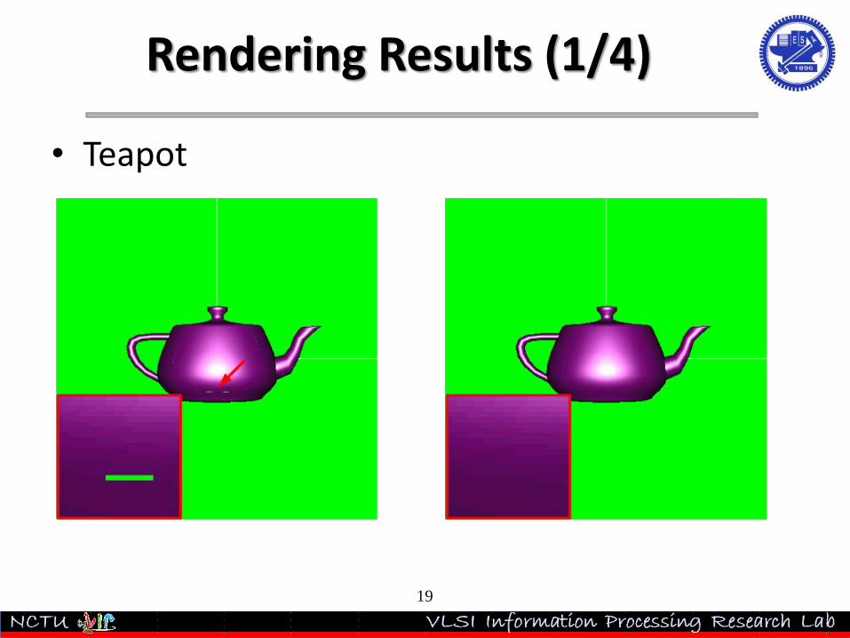
Rendering Results (1/4)
• Teapot
19
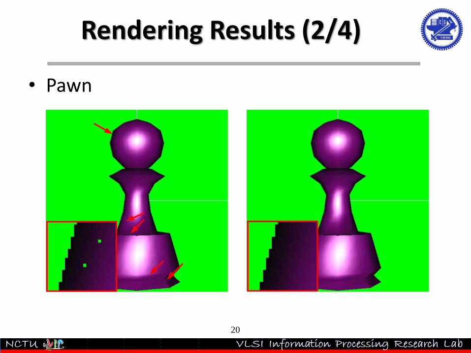
Rendering Results (2/4)
• Pawn
20

Rendering Results (3/4)
• Venus
21
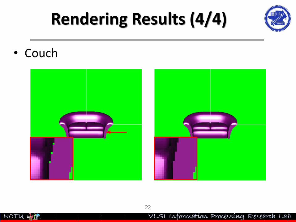
Rendering Results (4/4)
• Couch
22

Computation of Edge Function (1/2)
• Recovery scheme can reduce the complexity of evaluating the edge functions.
23
abbaab
abab
baab
abababab
yxyxC
xxB
yyA
C*yB*x: AE
**
0
bccbbc
bcbc
cbbc
bcbcbcbc
yxyxC
xxB
yyA
C*yB*x: AE
**
0
caacca
caca
acca
cacacaca
yxyxC
xxB
yyA
C*yB*x: AE
**
0
)**(2
1
))(*)()(*)((2
1
bcababbc
bcbaabbc
ab
BABA
yyxxyyxx
C
)**(2
1
))(*)()(*)((2
1
cabcbcca
cacbbcca
bc
BABA
yyxxyyxx
C
)**(2
1
))(*)()(*)((2
1
abcacaab
abaccaab
ca
BABA
yyxxyyxx
C
2 muls + 3 subs 2 muls + 1 subs

Computation of Edge Function (2/2)
• Evaluating one edge function requires:
– 2 multiplications + 3 subtractions = 2 muls + 3 adds
• For a triangle with NS segments on each edge, there are total 3NS
edge functions to be computed.
• Evaluating all edge functions for these triangles requires:
3*NS*(2 muls + 3 adds) = 6*NS muls + 9*NS adds
• With the proposed recovery scheme, the computation only requires:
3*(2 muls + 3 adds) + (3*NS-3) * (1 sub) + 3*(2 muls + 1 add)
= 12 muls + (3*NS+9) adds
24

Dual Space Subdivision (1/4)
• Transforms in GE
25
Modelview Transform(Object –> Eye)
Projection Transform(Eye–> Clip)
Perspective Division(Clip –> NDC)
Viewport Transform(NDC -> Window)
110001
34333231
24232221
14131211
object
object
object
eye
eye
eye
z
y
x
mmmm
mmmm
mmmm
z
y
x
1
0100
200
02
0
002
eye
eye
eye
clip
clip
clip
clip
z
y
x
nf
fn
nf
nfbt
bt
bt
nlr
lr
lr
n
w
z
y
x
clipclip
clipclip
clipclip
NDC
NDC
NDC
wz
wy
wx
z
y
x
/
/
/
offsetNDCscale
offsetNDCscale
offsetNDCscale
window
window
window
zzz
yyy
xxx
z
y
x

Dual Space Subdivision (2/4)
• Subdivide triangles in both eye space and window space– Reduce the computation of transforms
– Perspective incorrectly subdivision can be adopted if the error is acceptable.
26
Eye-space subdivision data flow:
Dual space subdivision data flow:

Dual Space Subdivision (3/4)
• Complexity analysis of the eye-space subdivision for one original triangle.– NGV: The number of the generated vertices.
27
Operations Computational Complexity
Modelview transform for 3 vertices 3x9 muls + 3x9 adds
Normal transform for 3 vertices 3x9 muls + 3x6 adds
Subdivision for 6 components :
Eye coordinate: (xeye, yeye, zeye)
Normal : (xN, yN, zN)
6(4L-1) adds
Projection transform for
NGV+3 vertices5(NGV+3) muls + 3(NGV+3) adds
Perspective division for
NGV+3 vertices3(NGV +3) muls + (NGV+3) invs
Viewport transform for
NGV +3 vertices3(NGV+3) muls + 3(NGV+3) adds
Total
(11 NGV+87) muls
(6 NGV+6x4L+ 57) adds
(NGV+3) invs

Dual Space Subdivision (4/4)
• Complexity analysis of the proposed dual space subdivision for one original triangle.
28
Operations Computational Complexity
Modelview transform for 3 vertices 3x9 muls + 3x9 adds
Normal transform for 3 vertices 3x9 muls + 3x6 adds
Projective transform for 3 vertices 3x5 muls + 3x3 adds
Perspective division for 3 vertices 3x3 muls + 3 invs
Viewport transform for 3 vertices 3x3 muls + 3x3 adds
Subdivision for 10 components:
Eye coordinate: (xeye, yeye, zeye)
Normal : (xN, yN, zN)
Window coordinate: 10(NGV +2) adds
Total
87 muls
(10 NGV +83) adds
3 invs
)1
,,,(clip
windowwindowwindoww
zyx

Triangle Setup Coefficient Sharing (1/3)
• Eliminate the unnecessary subdivision and setup operations for vertex attributes
29
Screen position
Texture coordinate
Depth value
Fog factor
1/w
Subdivider
Screen position
Eye space coordinate
Normal
Lighting unit
Sharing
setup
coefficient
Re-setup for
generated
triangles
3x3 matrix inverse and
matrix multiplication for
each attribute for a triangle 3x1matrix
multiplication for
each attribute

Triangle Setup Coefficient Sharing (2/3)
• Vertex attributes interpolation– Parameter ui– Perspective interpolation equation
30
Setup one attribute of a triangle requires one 3x3 matrix multiplication
Setup the coefficients of a triangle requires one 3x3 inverse matrix
iii
iii
iii
CyBxAu
CyBxAu
CyBxAu
222
111
000
111
][][ 210
210
210 yyy
xxx
CBAuuu iii
-1
210
210
210
111
][][
yyy
xxx
uuuCBA iii

Triangle Setup Coefficient Sharing (3/3)
• Level-1 case– Setup one attribute for 4 triangles require 4 3x3 inverse matrix and
multiplication.
• All subdivided triangles are on the same plane– Setup coefficients: Ai, Bi, Ci can be shared.
– Re-setup is required to compute initial point for each triangle.
31
Re-setup requires one 3x1 multiplication
1
][** y
x
CBACyBxAu iiiiii

• Notation definition:
– NT: The number of original visible triangles
– NOT: The number of original triangles for input models
– NGV: The number of new generated vertices in a subdivided triangle
– NA: The number of vertex attributes
– Example:
Complexity Analysis (1/4)
32

Complexity Analysis (2/4)
33
Conventional
subdivision
algorithm
Proposed
subdivision
algorithmUsed schemes
Number of memory accesses (4L+1-1)*NT (2NGV-2L+5)*NTForward
difference
Edge function
evaluation
Muls 6*NS*NT 12*NT Edge function
recovery Adds 9*NS*NT (3*NS+9)*NT
Computation for
transforms
Muls (11NGV+87)*NT 87*NTDual space
subdivisionAdds (6NGV+6x4L+ 57)*NT (10NGV+83)*NT
Invs (NGV+3) *NT 3*NT
Number of culling test
operations1*NOT 1*NOT
Triangle
filtering
Number of 3x3 matrix
multiplications for setupNA*NS
2*NT
Ceiling
{1/3*NA*NS2+NA}*
NT
Setup
coefficient
sharing

Complexity Analysis (3/4)
• Level-1 case with L=1, NGV=3, NA=5
34
Conventional
subdivision
algorithm
Proposed
subdivision
algorithm
Complexity
reduction
percentage
Number of memory accesses 15*NT 9*NT 40.00%
Edge function
evaluation
Muls 12*NT 12*NT 0%
Subs 18*NT 15*NT 16.67%
Computation for
transforms
Muls 120*NT 87*NT 27.50%
Adds 99*NT 113*NT -14.14%
Invs 6*NT 3*NT 50.00%
Number of 3x3 matrix
multiplications for setup20*NT 12*NT 40.00%

Complexity Analysis (4/4)
• Level-2 case with L=2, NGV=12, NA=5
35
Conventional
subdivision
algorithm
Proposed
subdivision
algorithm
Complexity
reduction
percentage
Number of memory accesses 63*NT 25*NT 68.88%
Edge function
evaluation
Muls 24*NT 12*NT 50.00%
Subs 36*NT 21*NT 41.67%
Computation for
transforms
Muls 219*NT 87*NT 60.27%
Adds 225*NT 203*NT 9.78%
Invs 15*NT 3*NT 80.00%
Number of 3x3 matrix
multiplications for setup80*NT 32*NT 60.00%

Proposed Power-Area Efficient Geometry Subsystem
• Proposed GE Architecture
• Proposed Primitive Processing Unit (PPU)
• Proposed Vertex Processing Unit (VPU)
– Reconfigurable Datapath (RDP)• light_dp
• trans_dp
• vec_norm
• pd
• POW
• vec_sub
36
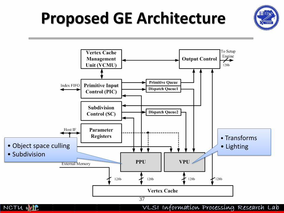
Proposed GE Architecture
37
• Transforms• Lighting • Object space culling
• Subdivision

Proposed GE Architecture
• Hardware feature
– Power-area efficient design• Achieve power-area efficiency (PAE): 545.1 Kvertices/(s*mW*mm2)
– Subdivision-based scalable shading quality support• Support level-0, level-1 and level-2
– High performance and area efficient vertex processing unit with reconfigurable datapath (RDP)• Speed up complicated operations. EX: vector normalization
• Hardware reusing
38

Proposed Primitive Processing Unit
39
d1=> Reg_Hdiff
d2=> Reg_Vdiff
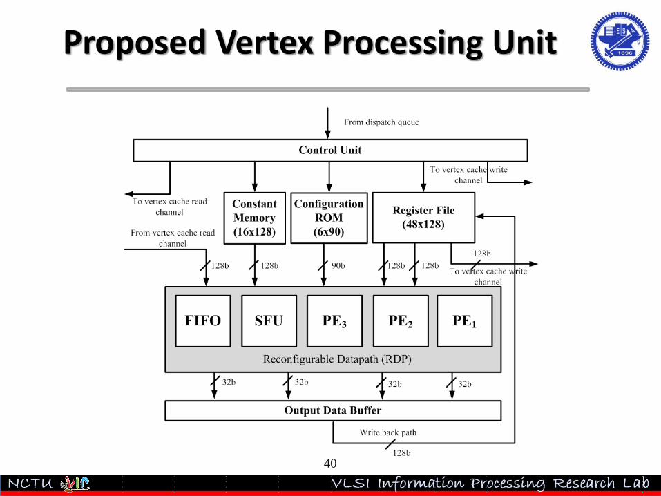
Proposed Vertex Processing Unit
40

Proposed Reconfigurable Datapath(RDP)
• Key components :
– Processing elements (PE)
– Special function unit (SFU)
– FIFO
• Configurations:
41
Configuration Modes Description
light_dp Dot product for lighting
trans_dp Dot product for transform
vec_norm Vector normalization
pd Perspective division
POW Powering
vec_sub Vector subtraction

Proposed Vertex Processing Unit
• Features
– High performance
• Peak transform performance: 50Mvertices/s
• Construct ASIC like datapath for high performance vertex processing via reconfigurable datapath.
– Area efficient
• Provide different operations for vertex processing with the same set of PEs.
42

Proposed Processing Element (PE)
43

Configuration inside PE
• MUL
44
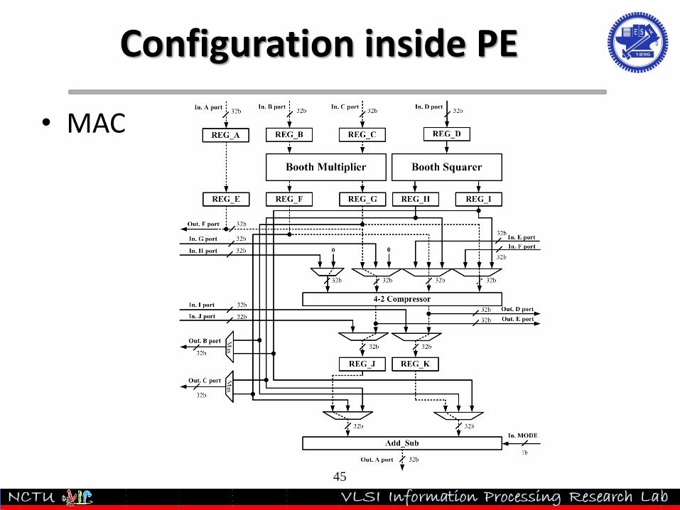
Configuration inside PE
• MAC
45

Configuration inside PE
• ADD/SUB
46

Configurations between PEs
• To clearly explain interconnection between PEs, a simplified block diagram PE is given.
47

Configurations between PEs
• light _dp
48
2*1+2*1+2*1=]2,2,2[•]1,1,1[ ZZYYXXZYXZYX

Configurations between PEs
• trans_dp
49
1+2*1+2*1+2*1=]1,2,2,2[•]1,1,1,1[ WZZYYXXZYXWZYX

Configurations between PEs
• vec_sub
50
]2,2,2[-]1,1,1[ ZYXZYX

Configurations between PEs
• vec_norm
51
222 111
]1
,1
,1
[])1,1,1([
ZYXLength
Length
Z
Length
Y
Length
XZYXnorm

Configurations between PEs
• Pd (perspective division)
52
]1
1,
1
1,
1
1[]1,1,1[
W
Z
W
Y
W
XZYX

Special Function Unit
• Log Number System and Operations:– Inverse
– Inverse square root
– Power (configured with 1 PE)
53

Chip Implementation Result
54
Power Supply 1.8V
Max. Clock 100 MHz
Max. Power 28.3 mW with level-1
Gate Count 183,748
Core Area 2.73 mm2
Process
Technology
TSMC 0.18 um
CMOS Process
VC ram1Ram2
Reg Bank
Constant Mem

Comparison Results
55
Level-0 Level-1 Level-2

Comparison Results
56
JSSC 2006 [2]
JSSC 2007 [3]
ISSCC 2007[4]
JSSC 2008 [5]
This Work
level-0 level-1 level-2
Process (nm) 180 180 180 180 180
Frequency (MHz) 200 100 200 50 100
Polygon Rate (Mvertices/s) 50 120 141 25*1/12.5*2 50*1/25*2
Power (mW) 155*3 157 52.4 8.6 28.3 33.6 43.6
Core Area (mm2) 23 16 9.7 6.05*4 2.73
Power-Area Efficiency (Kvertices/(s•mW•mm2)) 14 47.8 227 480.5 647.2 545.1 420.1
Feature Graphics Graphics Graphics Graphics, DSP
Graphics with scalable-quality hardware support
*1: With cache hit rate of 50%. *2: With cache hit rate of 0%.
*3: Include rendering engine. *4: With the core area of 2.164mmx2.797mm and see acknowledgement.
) (mm Core AreaPower (mW)
)Kvetices/sransform (Geomerty Trmance of Peak PerfoPAE
2

Conclusions
• Proposed an efficient subdivision algorithm • Low complexity
– The reduction of the number of memory accesses can be attained by 44.44% and 68.89% for level-1 and level-2, respectively.
– The reduction of the number of multiplications for transforms can be attained by 27.50% and 60.27% for level-1 and level-2, respectively.
• Scalable and near Phong shading quality
• Proposed power-area efficient geometry engine – Compared with [2-5], the proposed geometry engine has better power-area
efficiency with 545.1 Kvertices/(smWmm2) for level-1 subdivision.
– Compared with work in [5], the proposed geometry engine can increase the power-area efficiency by 34.7%, 13.4%, and -12.6% with level-0, level-1, level-2, respectively.
2018/9/1057

Reference
• [1] F. Arakawa et al., “An embedded processor core for consumer applications with 2.8 GFLOPS and 36 Mpolygons/s FPU,” IEEE ISSCC, Feb. 2004, pp. 334–335.
• [2] J. Sohn et al., “A 155-mW 50-Mvertices/s graphics processor with fixed-point programmable vertex shader for mobile applications,” IEEE J. Solid-State Circuits, vol. 41, no. 5, pp. 1081–1091, May 2006.
• [3] C. H. Yu, K. Chung, D. Kim and L. S. Kim, "An Energy-Efficient Mobil Vertex Processor With Multithread Expanded VLIW Architecture and Vertex Caches," IEEE J. Solid-State Circuits, vol. 42, no. 10, Oct. 2007.
• [4 ]B. G. Nam, J. Lee, K. Kim, S. J. Lee, and H.-J. Yoo, “A 52.4 mW 3-D graphics processor with 141 Mvertices/s vertex shader and 3 power domains of dynamic voltage and frequency scaling,” ISSCC 2007, pp. 278-603.
• [5 ]S. Y. Chien, Y. M. Tsao, C. H. Chang and Y. C. Lin, “An 8.6 mW 25 Mvertices/s 400-MFLOPS 800-MOPS 8.91 mm2 Multimedia Stream Processor Core for Mobile Applications,“ IEEE J. Solid-State Circuit, vol. 43, issue. 9, pp. 2025-2035, Sep. 2008.
58