- 21 -

Geometry, to appear in 1991.

[To92] Toussaint, G. T., ed.,Proceedings of the IEEE, Special Issue on Computational Geo-metry, to appear in 1992.

[YKII88] Yamamoto, P., Kato, K., Imai, K. and Imai, H., “Algorithms for vertical and orthogonallinear L1 approximation of points,” Proc. of the ACM Symp. on Computational Geo-

metry, Urbana-Champaign, 1988, pp. 352-361.

- 20 -

on Computational Geometry, Berkeley, 1990, pp. 211-215.

[Sh78] Shamos, M. I., “Computational geometry,” Ph.D. thesis, Yale University, May 1978.

[SH75] Shamos, M. I. and Hoey, D., “Closest-point problems,”16th Annual IEEE Symposiumon Foundations of Computer Science, October 1975, pp. 151-162.

[SSH87] Schwartz, J. T., Sharir, M., and Hopcroft, J.,Planning, Geometry, and the Complexityof Robot Motion, Norwood, 1987.

[St1882] Steiner, J.,Gesammelte Werke, 2. Bd. Berlin 1882, p. 45.

[St1884] Sturm, R., “Bemerkungen und Zusatze zu Steiners Aufsazen uber Maxima und Mini-ma,” Journal fur reine und angewande Mathematik, vol. 96,1884, pp.36-77.

[SY87] Schwartz, J. T. and Yap, C. K.,Algorithmic and Geometric Aspects of Robotics, Er-lbaum, 1987.

[Sy1857] Sylvester, J. J., “A question in the geometry of situation,”Quarterly Journal of Mathe-matics, vol. 1, 1957, p. 79.

[To83a] Toussaint, G. T., “Solving geometric problems with the rotating calipers,”Proc. ofIEEE MELECON, Athens, 1983.

[To83b] Toussaint, G. T., “Computing largest empty circles with location constraints,”Interna-tional Journal of Computer and Information Sciences, vol. 12, October 1983, pp. 347-358.

[To86] Toussaint, G. T., “An Optimal Algorithm for Computing the Relative Convex Hull ofa Set of Points in a Polygon, “Signal Processing III: Theories and Applications, Proc.of EURASIP-86, Part 2, The Hague, September 1986.

[To85a] Toussaint, G. T., “A historical note on convex hull finding algorithms,”Pattern Reco-gnition Letters, vol. 3, January 1985, pp. 21-28.

[To85b] Toussaint, G. T., ed.,Computational Geometry, North-Holland, 1985.

[To88a] Toussaint, G. T., ed.,Computational Morphology, North-Holland, 1988.

[To88b] Toussaint, G. T., ed.,The Visual Computer, Special Issue on Computational Geometry,vol. 3, No. 6, May 1988.

[To89] Toussaint, G. T., “Computing geodesic properties of polygons,”Revue D’IntelligenceArtificielle, vol. 3, 1989, pp. 9-42.

[To90b] Toussaint, G. T.,Workshop on Illuminating Sets, Bellairs Research Inst. of McGillUniv., Feb. 1990.

[To90a] Toussaint, G. T., “An output-complexity-sensitive polygon triangulation algorithm,”Proc. Computer Graphics International’90, Singapore, June 1990, pp. 443-466.

[To91] Toussaint, G. T., ed.,Pattern Recognition Letters, Special Issue on Computational

- 19 -

rithmica, vol. 1, pp. 193-211

[Me83] Megiddo, N., “Linear time algorithm for linear programming inR3 and related prob-lems,”SIAM Journal of Computing, vol. 12, November 1983, pp. 759-776.

[Me84] Megiddo, M., “Linear programming in linear time when the dimension is fixed,”Jour-nal of the Association for Computing Machinery, vol. 31, 1984, pp. 114-127.

[Me89] Megiddo, M., “On the ball spanned by balls,”Discrete and Computational Geometry,vol. 4, 1989, pp. 605-610.

[Meh84] Mehlhorn, K.,Multidimensional Searching and Computational Geometry, Springer-Verlag, 1984.

[MN80] Morris, J. G. and Norback, J. P., “A simple approach to linear facility location,”Trans-portation Science, vol. 14, 1980, pp. 1-8.

[MS90] Melissaratos, E. A. and Souvaine, D. L., “On Solving Geometric Optimization Prob-lems Using Shortest Paths,”Proc. of the ACM Symp. on Computational. Geometry,Berkeley, 1990, pp. 350-359.

[Ni81] Niven, I., Maxima and Minima Without Calculus, The Mathematical Association ofAmerica, 1981, p. 163.

[O83] O’Rourke, J., “An on-line algorithm for fitting lines between data ranges,”Communi-cation of the ACM, 24, 1981, pp. 574-578.

[O’R87] O’Rourke, J.,Art Gallery Theorems and Algorithms, Oxford University Press, 1987.

[Pr77] Preparata, F. P., “Minimum spanning circle,” inSteps into Computational Geometry,F. P. Preparata, ed., University of Illinois, March 1977, pp. 3-5.

[Pr83] Preparata, F., ed.,Computational Geometry, JAI Press, 1983.

[PS85] Preparata, F. P. and Shamos, M. I.,Computational Geometry, Springer-Verlag, 1985.

[PS86] Pollack, R., Sharir, M., “Computing the geodesic center of a simple polygon,” inProc.Workshop on Movable Separability of Sets, G. Toussaint,ed., Bellairs Research Insti-tute, Barbados, February 1986.

[PSR89] Pollack, R., Sharir, M., and Rote, G., “Computing the geodesic center of a simple poly-gon,” J. of Discrete and Comp. Geometry, Vol.4, No. 6, 1989, pp. 611-626.

[RT57] Rademacher, H. and Toeplitz, O.,The Enjoyment of Mathematics, Princeton UniversityPress, 1957.

[Sc1890] Schwarz, H. A., Gesammelte Mathematische Abhandlungen, 2. Bd., Berlin 1890, pp.344-345.

[Se90] Seidel, R., “Linear programming and convex hulls made easy,”Proc. of the ACM Symp.

- 18 -

tures, Lecture Notes in Computer Science 382, F. Dehne, J.-R. Sack and N. Santoroeds., Springer-Verlag, 1989, pp. 183-191.

[HR88] Houle, M. E. and Robert J.-M., “Orthogonal weighted linear approximation and appli-cations,” Tech. Rept. SOCS-88.13, McGill University, August 1988.

[HS86] Hart, and Sharir, M., “Nonlinearity of Davenport-Schintzel sequences and of general-ized path compression schemes,” Combinatorica, 6, 1986, pp.151-177.[H]Hershberg-er, J., “Finding the upper envelope of n line segments in O(n log n) time,” InformationProcessing Letters, vol. 33, 1989, pp. 169-184.

[HS] Hershberger, J. and Suri, S., “Off-line maintenance of planar configurations,” SODA,San Francisco, January 1991.

[HT88] Houle, M. E. and Toussaint, G. T., “Computing the width of a set,” IEEE Transactionsin Pattern Analysis and Machine Intelligence, vol. 10, 1988, pp. 761-765.

[HT85] Hildebrandt, S. and Tromba, A., Mathematics and Optimal Form, Scientific AmericanBooks, Inc., 1985, p. 60.

[IKY89] Imai, H., Kato, K. and Yamamoto, P., “A linear-time algorithm for linear L1 approxi-

mation of points,” Algorithmica, vol. 4, 1989, pp. 77-96.

[KET90] Kong, X., Everett, H. and Toussaint, G. T., “Graham scan triangulates a simple poly-gon,” Pattern Recognition Letters, in press.

[KK85] Karzakis, J. and Karagiorgis, P., “A method to locate the maximum circle inscribed ina polygon, “Belgian Journal of Operations Research, Statistics and Computer Sci-ence,” vol. 26, No. 3. 1985, pp. 3-36.

[Kl89] Klein, R., Concrete and Abstract Voronoi Diagrams, Springer-Verlag, 1989.

[KR85] Klotzler, R. and Rudolph, H., “Zur analytischen und algorithmischen Behandlung einesgeometrischen Optimierungsproblems von J. Steiner,” Optimzation, vol. 16, 1985, pp.833-848.

[LD81] Lee, D. T. and Drysdale III, R. L., “Generalizations of Voronoi diagrams in the plane,”SIAM Journal on Computing, vol. 10, 1981, pp. 73-87.

[Le80] Lee, D. T., “Farthest neighbor Voronoi diagrams and applications,” Tech. Rept. #80-11-FC-04, Northwestern University, November 1980.

[Le82] Lee, D. T., “Medial axis transformation of a planar shape,” IEEE Transactions on Pat-tern Analysis and Machine Intelligence, vol. PAMI-4, July 1982, pp. 363-369.

[LP84] Lee, D. T., and Preparata, F. P., “Euclidean shortest paths in the presence of rectilinearbarriers,” Networks, Vol. 14, No. 3., 1984, pp. 393-410.

[LS87] Leven, D. and Sharir, M., “Intersection and proximity problems and Voronoi dia-grams,” in Algorithmic and Geometric Aspects of Robotics Volume 1, J. T. Schwartzand C.-K. Yap eds., Lawrence Ertlbaum Associates, 1987, pp. 187-228.

[LW86] Lee, D. T. and Wu, Y. F., “Geometric complexity of some location problems,” Algo-

- 17 -

1989.

[CN86] Chin, W. and Ntafos, S., “Optimum watchman routes,” Proc. of the ACM Symp. onComputational Geometry, Yorktown Heights, 1986, 24-33.

[CR41] Courant, R. and Robbins, H., What is Mathematics?, Oxford Univ. Press, 1941, 346-352.

[DT81] Devroye, L. and Toussaint, G. T., “A note on linear expected time algorithms for find-ing convex hulls,” Computing, vol. 26, pp. 361-366

[Dy86] Dyer, M. E., “On a multidimensional search technique and its applications to the Eu-clidean one-center problem,” SIAM Journal on Computing, vol. 15, 1986, pp. 725-738.

[Ed85] Edelsbrunner, H., “Finding transversals for sets of simple geometric figures,” Theoret-ical Computer Sciences, vol. 35, 1985, pp. 55-69.

[Ed87] Edelsbrunner, H., Algorithms in Combinatorial Geometry, Springer-Verlag, 1987.

[EG89] Edelsbrunner, H. and Guibas, L. J., “Topologically sweeping an arrangement,” Journalof Computer and System Sciences, vol 38, 1989, pp. 165-194.

[EH72] Elzinga, J. and Hearn, D. W., “Geometrical solutions for some minimax location prob-lems,” Transportation Science, vol. 6, 1972, pp. 379-394.

[EMPRWW82] Edelsbrunner, H., Maurer, H. A., Preparata, F. P., Rosenberg, A. L., Welzl, E.and Wood, D., “Stabbing line segments,” BIT, vol. 22, 1982, pp. 274-281.

[ET90] Everett, H. and Toussaint, G. T., “Illuminating objects in the plane with point lightsources,” Proc. Third Australasian Workshop on Combinatorial Algorithms, Ubud, In-donesia, June 11-15, 1990.

[EW89] Egyed, P. and Wenger, R., “Stabbing pairwise disjoint translates in linear time,” Proc.of the ACM Symp. on Computational Geometry, Saarbruchen, 1989, pp. 364-369.

[Fo86] Focke, J., “A finite descent method for STEINER’s problem of inpolygons with mini-mal circumference,” Optimization, 17, 1986, pp. 355-366.

[FM84] Fournier, A. and Montuno, D. Y., “Triangulating Simple Polygons and EquivalentProblems,” ACM Transactions on Graphics, 1984, 153-74.

[FW74] Francis, R. L. and White, J. A., Facility Layout and Location: An Analytical Approach,Prentice-Hall, Inc., 1974.

[GSLHT87] Guibas, L., Hershberger, J., Leven, D., Sharir, M. and Tarjan, R. E., “Linear Time Al-gorithms for Visibility and Shortest Path Problems Inside Triangulated Simple Poly-gons,” Algorithmica, vol. 2, 1987, 209-233.

[He89] Hershberger, J., “Finding the upper envelope of n lines segments in O(n log n) time,”Information Processing Letters, vol. 33, 1989, pp. 169-174.

[HIIR89] Houle, M. E., Imai, H., Imai, K. and Robert J.-M., “Weighted orthogonal linear L∞-ap-

proximation and applications,” Proc. of the Workshop on Algorithms and Data Struc-

- 16 -

65-79.

[AT78] Akl, S. G. and Toussaint, G. T., “Efficient convex hull algorithms for pattern recogni-tion applications,” Proc. Fourth International Joint Conf. on Pattern Recognition, Ky-oto, Japan, 1978.

[AT81] Avis, D. and Toussaint, G. T., “An efficient algorithm for decomposing a simple poly-gon into star-shaped pieces,” Pattern Recognition, vol. 13, 1981, pp. 295-298.

[Ba84] Bajaj, C., “Geometric optimization and computational complexity,” Ph.D. thesis, Tech.Rept. TR-84-629, Cornell University, 1984.

[BCEKSTU90] Bhattacharya, B. K., Czyzowics, J., Egyed, P., Keil. M., Stojmenovic, I., Tous-saint, G. T. and Urrutia, J., “Computing shortest transversals of sets,” manuscript inpreparation.

[BE86] Bhattacharya, B. K. and ElGindy H., “An efficient algorithm for an intersection prob-lem and an application,” Tech. Rept. No. 86-25, Dept. of Computer and InformationScience, University of Pennsylvania, April 1986.

[BS67] Bass, L. J. and Schubert, S. R., “On finding the disc of minimum radius containing agiven set of points,” Mathematics of Computation, vol. 21, 1967, pp. 712-714.

[BT83] Bhattacharya, B. K. and Toussaint, G. T., “Time-and-storage-efficient implementationof an optimal planar convex hull algorithm,” Image and Vision Computing, vol. 1, no.3, August 1983, pp. 140-144.

[BT85] Bhattacharya, B. K. and Toussaint, G. T., “On geometric algorithms that use the fur-thest-point Voronoi diagram,” in Computational Geometry, ed., G. T. Toussaint,North-Holland, 1985, pp. 43-61.

[BT90] Bhattacharya, B. K. and Toussaint, G. T., “Computing shortest transversals,” Compu-ting, in press.

[BCEKSTU] Bhattacharya, B., Czyzowics, J., Egyed, P., Stojmenovic, I., Toussaint, G. T., Urru-tia, J., “Computing shortest transversals,” manuscript in preparation.

[CEERSSTU90] Czyzowics, J., Egyed, P., Everett, H., Rappaport, D., Shermer, T., Souvaine, D.,Toussaint, G. T. and Urrutia, J., “The aquarium keeper’s problem,” SODA, San Fran-cisco, January 1991.

[Ch82] Chazelle, B., “A theorem on polygon cutting with applications,” Proc. 23rd IEEESymp. on Foundations of Computer Science, Chicago, Nov. 1982, pp. 339-349.

[Ch90] Chazelle, B., “Triangulating a simple polygon in linear time,” Technical Report CS-TR-264-90, Princeton Univ., May 1990.

[Ch75] Chvatal, V., “A combinatorial theorem in plane geometry,” Journal of CombinatorialTheory, Series B, vol. 18, 1975, pp. 39-41.

[CN89] Chin, W. and Ntafos, S., “Optimum zoo-keeper routes,” Congressus Numerantium,

- 15 -

tion principle and shortest-path maps. They also generalize their method by using relative convexhulls [To86] to provide a linear-time algorithm for polygons which are not convex. Chin and Nta-fos [CN86] have used a somewhat similar combination of the reflection principle and shortest-paths to solve a related problem of computing shortest watchman routes in rectilinear polygons.

The Aquarium Keeper’s Problem is related to another problem considered by Chin andNtafos [CN89], the Zoo Keeper’s Problem. In the Zoo Keeper’s Problem, given a simple polygonP of n vertices, k convex polygons (cages) attached to edges of P, and an entry point x on the bound-ary of P, the goal is to find the minimum perimeter tour in P and not in the interior of any cage,

starting and ending at x, that visits every cage. Their paper contains an O(n logk n) time algorithm

and refers to an O(n2) algorithm for the problem as well. If we consider the cages as edges of P,i.e., the edges of P represent the front glass plates of a series of aquariums and have n cages, thenthe Zoo Keeper’s Problem reduces to a simplified version of the Aquarium Problem in which afixed starting point is given. Note that even without this restriction, the complexity of the algorithm

in [CEERSSTU90] is appreciably less than either O(n logk n) or O(n2).

6. Multiple Facility Location of the Visibility Kind

Consider a large warehouse in which it is desired to install a surveillance system consistingof a set of cameras. The cameras are to be installed in fixed positions but are allowed to rotatethrough 360°. It is required that every portion of the warehouse fall in the field of view of at leastone camera as it makes a full revolution. On the other hand we don’t want to install too many cam-eras to do the job. This is an example of a multiple-facility location problem of the visibility kindwhere the facilities are points (camera locations) and the warehouse is the “customer.” We canmodel the warehouse as a simple polygon of n vertices in the plane. A well known theorem thatconcerns this type of multiple-facility location problem is Chvatal’s Art-Gallery Theorem[O’R87]. This theorem states that n/3 cameras are always sufficient and sometimes necessary todo the job [Ch75]. Avis and Toussaint [AT81] presented an O(n log n) time algorithm for findingthe location of these cameras. The book by O’Rourke [O’R87] is devoted entirely to these types offacility location problems for simple polygons as customers. For the case of simple objects such ascircles and squared as customers a survey of results can be found in [ET90].

7. References

[AB87] Atallah, M. and Bajaj, C., “Efficient algorithms for common transversals,” InformationProcessing Letters, vol. 25, 1987, pp. 87-91.

[ARW89] Avis, D., Robert, J.-M. and Wenger, R., “Lower bounds for line stabbing,” InformationProcessing Letters, vol. 33, 1989, pp. 59-62.

[AT85] Asano, T. and Toussaint, G. T., “Computing the geodesic center of a simple polygon,”Technical Report SOCS-85.32, McGill University, 1985.

[AT86] Asano, T. and Toussaint, G. T., “Computing the geodesic center of a simple polygon,”in Perspectives in Computing: Discrete Algorithms and Complexity, Proc. of Japan-USJoint Seminar, D. S. Johnson, A. Nozaki, T. Nishizeki, H. Willis, eds., June 1986, pp.

- 14 -

calipers. Finally, if the line segments are already sorted, the running time of the algorithm is O(n).

5. Polygonal Facilities

Just as we may have a point facility in a polygonal customer [KK85] we may also have apolygonal facility with different types of customers. The polygonal facility can be viewed as a cir-cuit of railway lines for example or a circuit of power lines to provide electricity to a polygonalregion, etc. When the customers are points then we of course obtain the old and famous travellingsalesman problem which is well known and hence we do not consider here. Much more novel isthe situation where the customer is itself a simple polygon or a set of convex polygons lying in theinterior of a simple polygon and we briefly touch upon this topic below.

Although variously attributed to Fagnano [Ni81] and Steiner [Fo86], [KR85], [St1884],[St1882], many sources insist that, over one hundred years ago, Schwarz [Sc1890] not only solvedthe problem of computing the minimum perimeter triangle with one vertex on each edge of a giventriangle but that he also posed the problem. In any case, there is consensus that Schwarz used thereflection principle to show that the foot points of the altitudes of an acute triangle are the verticesof the minimum inscribed polygon. For obtuse triangles, the minimum perimeter inscribed trian-gle is realized by twice the shortest altitude, i.e., it is degenerate with two vertices coinciding withthe obtuse vertex of the input triangle. In 1985, Klotzler and Rudolph [KR85] used a semi-infinitesimplex-method to determine the minimum perimeter polygon with one vertex on each edge of agiven convex polygon, or the minimum perimeter inpolygon. In 1986, Focke [Fo86] presented analgorithm for computing the optimum inpolygon, using a finite descent method resulting fromSchwarz’ reflection principle and coordinate-wise descent. He presents four examples to illustrateefficient performance of the algorithm, but provides no formal complexity analysis. In addition,his classification of correct solutions omits one realizable type and it is unclear whether his algo-rithm would in fact detect the correct solution.

At a recent workshop, Toussaint [To90b] posed the problem somewhat differently: heasked for the shortest closed path inside a simple polygon (Aquarium Keeper’s Tour) which visitsevery edge at least once. If the polygon is convex, then the optimum path is, in fact, the minimumperimeter inpolygon, and [CEERSSTU90] present a linear-time algorithm which uses the reflec-

a aa

b b

b

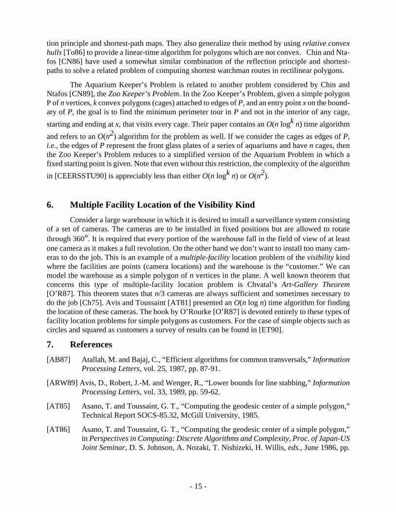
(a) aba impossible (b) abab impossible (c) ababa impossible

Fig. 5

- 13 -

the list θ0 = 0°, θ1, θ2..., θs-1, θs = 90°.

Step 3: Set i = 0.

Step 4: Compute CH(UP(F, θi)) and CH(LH(F, θi).

Step 5: Find the thinnest strip transversal with orientation θ s. t. θi ≤ θ ≤ θi+1.

Step 6: Update CH(UP(F, θi)) and CH(LH(F, θi) and produce CH(UP(F, θi+1)) and

CH(LH(F, θi+1).

Step 7: Let i = i + 1. If i < s, go to 5.

Step 8: Output the thinnest strip overall the strips found in Step 5.

The crucial point of this algorithm for its running time is the convex hull updating in Step6. By using the recent algorithm by Hershberger and Suri [HS91], it is possible to do the O(n) in-sertions and deletions in O(log n) amortized time per operation when all the points to be processedare known in advance. Then, since Step 1 can be done in O(n) time using the rotating calipers al-gorithm, as mentioned before, and Steps 2 and 3 and all the convex hull updates in O(n log n) time,the algorithm runs in O(n log n + p) time where p is the number of vertices visited by the rotatingcalipers algorithm in Step 5.

An upper bound on p can be derived from the theory of Davenport-Schintzel sequences.The sequence of all vertices visited in Step 5 by the lower tangents form a sequence of labels suchthat no two adjacent symbols are the same and, furthermore, it is impossible to have the subse-quence a...b...a...b...a. Fig. 5 illustrates all the different cases. In case 3(c), for example, it is pos-sible to have the sequence a...b...a...b. To obtain the sequence a...b...a...b, the tangent has to havean orientation greater than that of the edge containing the vertex a. So, the vertex a is replaced bythe other endpoint and it will never be looked at again. Therefore the sequence a...b...a...b...a willnever appear. Thus, the sequence of vertices corresponds to a (n, 3)-Davenport-Schintzel sequenceand the O(n α(n)) upper bound of Hart and Sharir [HS86], where α(n) is the functional inverse ofAckermann’s function, gives an upper bound on p. Therefore, the overall running time of the algo-rithm is O(n log n). For vertical line segments, the algorithm consists of only one phase of comput-ing the convex hulls of the tangent points and finding the thinnest strip transversal with the rotating

a

bc

b

a

(a) (b)Fig. 4

- 12 -

orientation between 0° and 90° only. To solve the unrestricted problem, the algorithm should beused twice.

The algorithm can be divided into two parts: finding the thinnest strip between two consec-utive critical directions and updating the information needed to find the strip transversal. Since thetangent points do not change between two adjacent critical directions, say θ1 and θ2, the thinnest

strip transversal can be compute easily in that range. When the convex hulls of the upper tangentpoints CH(UP(F, θ1)) and the lower tangent points CH(LP(F, θ1)) have been computed, the thin-

nest strip transversal can be found by determining the lower tangent tl(CH(UP(F, θ1), θ1)) and the

upper tangent tu(CH(LP(F, θ1), θ1)) and rotating them until they have an orientation θ2 [HT88].

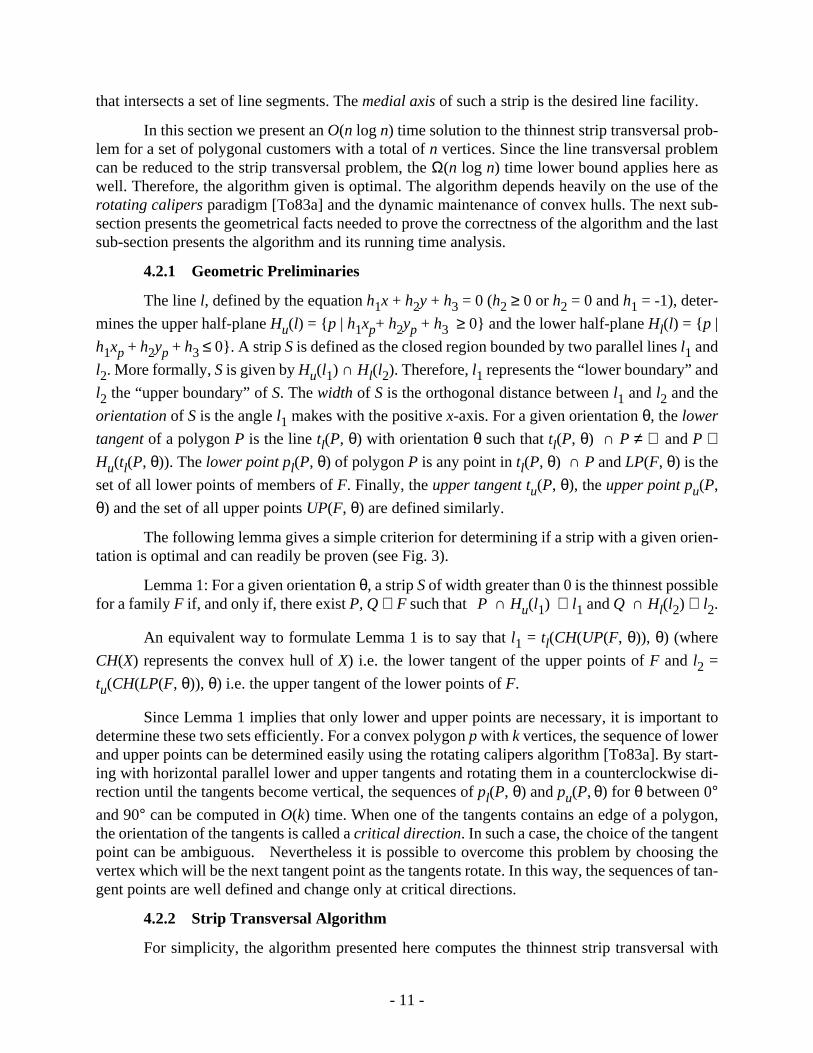
Note that if, at any moment, the lower tangent becomes “above” or “on” the upper tangent, a linetransversal (i.e. a strip with width 0) is found. Finally, the extreme case where the tangents haveorientation θ2 should be looked at carefully. Even if UP(F, θ1) ≠ UP(F, θ2), the lower tangents

tl(CH(UP(F, θ1), θ2) and tl(CH(UP(F, θ2), θ2) are the same since UP(F, θ2) = (UP(F, θ1)) \ a)

∪ b, where [a, b] is an edge of one member of F and has an orientation θ2 (if many edges are

parallel more than one point can be replaced at the same time). Fig. 4 illustrates the two caseswhich can occur. The segment [a, b] either belongs to the lower tangent or it does not. In eithercase, replacing the point a by b does not affect the tangent. Furthermore, this gives a simple wayto update CH(UP(F, θ1)) to obtain CH(UP(F, θ2)). One point should be added and one should be

deleted from the convex hull. Naturally, theses observations also hold for CH(LP(F, θ2)) and

tu(CH(LP(F, θ2), θ2)).

From the above facts, the algorithm is simply a succession of subproblems consisting offinding the thinnest strip transversal in a given orientation range and updating all the informationto be able to process efficiently the next range. The algorithm can now be stated as follows:

Strip Transversal Algorithm:

Step 1: Compute the sequence of tangent points for each member of F.

Step 2: Compute the critical directions and sort them according to their slopes to produce

l2 l1

Q

PHu (l1) ∩ Hl (l2)

Fig. 3 Illustrating the proof of Lemma 1.

- 11 -

that intersects a set of line segments. The medial axis of such a strip is the desired line facility.

In this section we present an O(n log n) time solution to the thinnest strip transversal prob-lem for a set of polygonal customers with a total of n vertices. Since the line transversal problemcan be reduced to the strip transversal problem, the Ω(n log n) time lower bound applies here aswell. Therefore, the algorithm given is optimal. The algorithm depends heavily on the use of therotating calipers paradigm [To83a] and the dynamic maintenance of convex hulls. The next sub-section presents the geometrical facts needed to prove the correctness of the algorithm and the lastsub-section presents the algorithm and its running time analysis.

4.2.1 Geometric Preliminaries

The line l, defined by the equation h1x + h2y + h3 = 0 (h2 ≥ 0 or h2 = 0 and h1 = -1), deter-

mines the upper half-plane Hu(l) = p | h1xp+ h2yp + h3 ≥ 0 and the lower half-plane Hl(l) = p |

h1xp + h2yp + h3 ≤ 0. A strip S is defined as the closed region bounded by two parallel lines l1 and

l2. More formally, S is given by Hu(l1) ∩ Hl(l2). Therefore, l1 represents the “lower boundary” and

l2 the “upper boundary” of S. The width of S is the orthogonal distance between l1 and l2 and the

orientation of S is the angle l1 makes with the positive x-axis. For a given orientation θ, the lower

tangent of a polygon P is the line tl(P, θ) with orientation θ such that tl(P, θ) ∩ P ≠ ∅ and P ⊂Hu(tl(P, θ)). The lower point pl(P, θ) of polygon P is any point in tl(P, θ) ∩ P and LP(F, θ) is the

set of all lower points of members of F. Finally, the upper tangent tu(P, θ), the upper point pu(P,

θ) and the set of all upper points UP(F, θ) are defined similarly.

The following lemma gives a simple criterion for determining if a strip with a given orien-tation is optimal and can readily be proven (see Fig. 3).

Lemma 1: For a given orientation θ, a strip S of width greater than 0 is the thinnest possiblefor a family F if, and only if, there exist P, Q ∈ F such that P ∩ Hu(l1) ⊆ l1 and Q ∩ Hl(l2) ⊆ l2.

An equivalent way to formulate Lemma 1 is to say that l1 = tl(CH(UP(F, θ)), θ) (where

CH(X) represents the convex hull of X) i.e. the lower tangent of the upper points of F and l2 =

tu(CH(LP(F, θ)), θ) i.e. the upper tangent of the lower points of F.

Since Lemma 1 implies that only lower and upper points are necessary, it is important todetermine these two sets efficiently. For a convex polygon p with k vertices, the sequence of lowerand upper points can be determined easily using the rotating calipers algorithm [To83a]. By start-ing with horizontal parallel lower and upper tangents and rotating them in a counterclockwise di-rection until the tangents become vertical, the sequences of pl(P, θ) and pu(P, θ) for θ between 0°and 90° can be computed in O(k) time. When one of the tangents contains an edge of a polygon,the orientation of the tangents is called a critical direction. In such a case, the choice of the tangentpoint can be ambiguous. Nevertheless it is possible to overcome this problem by choosing thevertex which will be the next tangent point as the tangents rotate. In this way, the sequences of tan-gent points are well defined and change only at critical directions.

4.2.2 Strip Transversal Algorithm

For simplicity, the algorithm presented here computes the thinnest strip transversal with

- 10 -

presented in the past. Houle and Toussaint [HT88] solved the unweighted case, Edelsbrunner[Ed85] claimed to be able to solve the weighted case optimally and, finally, Houle et al. [HIIR89]also presented an optimal solution for the weighted case which can be extended to higher dimen-sions. For the L1-norm, Houle and Robert [HR88] and Yamamoto et al. [YKII88] presented two

different O(n2) time algorithms both based on performing a topological sweep of an arrangementof hyperplanes [EG89]. The first algorithm can be used to solve the problem in higher dimensionsand the second can be transformed to solve the unweighted case in O(n1.5 log2 n) time.

4.2 Simple convex objects as customers

The line-facility location problem for simple-convex-customers has been solved in a verynarrow setting in the past. It corresponds to the line transversal problem investigated in both themathematics [DGK63], [HDK64] and computer science [AB87], [Ed85], [EW89] literatures. LetS be a family of convex sets. The line transversal problem consists of finding a line which intersectseach member of S if it exists.

For a family of n simple convex objects, by combining the algorithms of Atallah and Bajaj[AB87] and Hershberger [He89], it is possible to find a line transversal in O(n log n) time. Recent-ly, Avis, Robert and Wenger [ARW90] proved that such an algorithm is optimal. When the objectsare restricted to be mutually disjoint translates of a convex set, Egyed and Wenger [EW89] gavean optimal linear time algorithm to solve the problem. For line segments, Edelsbrunner and Guibas[EG89] gave an O(n2) time algorithm to find a line which intersects the maximum number of themby sweeping the line arrangement in the dual space. The same method will work for a family ofconvex polygons with a fixed number of vertices.

Recently, Bhattacharya and Toussaint [BT90] introduced the problem of computing theshortest line segment transversal for a family of line segments. This problem can be interpreted asfinding the smallest line-segment-facility which intersects each line-segment-customer. They pro-posed a O(n log n) time algorithm to find such a transversal for a set of non-intersecting line seg-ments. They also gave a O(n log2 n) time algorithm for a set of lines or, possibly intersecting, linesegments. Bhattacharya et al. [BCEKSTU90] improved this result and obtained an optimal O(n logn) time algorithm for a family of line segments. They also presented an O(n log n) time algorithmfor a set of lines, but the optimality of this algorithm has not yet been determined. It should bepointed out here that if it is desired to find the shortest vertical line segment facility which inter-sects each of n line-customers then the problem is identical to the point-facility for lines as custom-ers using the Euclidean vertical distance. As pointed out in sub-section 3.2 this problem can be ex-pressed as a linear program in three variables and can thus be solved in O(n) time.

The line-facility location for simple-object-customers appears not to have been examinedbefore. For example, suppose we have n line segments which represent the customers, one possibleproblem is to find the line which minimizes the maximum Euclidean orthogonal distance betweena line segment and the line. Equivalently, the problem can be stated as finding the thinnest strip

- 9 -

only the two following facts:

i) FPVD(S) consists of at most a linear number of edges and vertices,

ii) each edge is a connected subset of a bisector between two sites (i.e. the locus of pointswhich are equidistant from two sites).

An optimal solution of the point-facility location problem must belong to the FPVD of thecustomers since at least two customers must be externally tangent to the circle corresponding tothe solution. Therefore, for mutually disjoint line-segment-customers, Fortune’s algorithm [Fo87]can compute the FPVD in O(n log n) time and the solution can then be found in linear time by ex-amining the vertices and the “edges” each of which is composed of at most seven straight line seg-ments and parabolic arcs. For more complex customers, we have to be more careful. If the custom-er sites have to many vertices, the edges of the FPVD can be formed by too many segments andthe last part of the algorithm will take more than linear time. If we restrict the customers to be smallconvex polygons with a fixed upper bound on the number of vertices, the algorithm will still findthe solution in linear time from the FPVD. However, it is no longer possible to compute the FPVDin O(n log n) time and we have to resort to Lee and Drysdale’s algorithm [LD81] which runs inO(n log2 n) time. The special case of circle-customers can be solved easily using linear program-ming. Megiddo [Me89] presented a linear time algorithm to solve this problem in any fixed dimen-sion.

4. Line-Facility Location

The general formulation of the last section still applies in this case. The only difference willbe in the definition of the distance function between the customers and the line-facility.

4.1 Points as customers

The line-facility location problem for point-customers is simply the well known line-fittingor linear approximation problem. Many solutions have been presented over the years for the dif-ferent norms and distance metrics used.

For the Euclidean vertical distance, it is possible to solve the problem optimally for the L1,

L2 (the summation of the squared distance) and L∞-norms. The problem with the L∞-norm can be

formulated as a three-variable linear programming problem and can be solved in linear time [Dy86,Me84]. The problem can also be solved optimally in any fixed dimension. The well known least-squares method finds the solution for the L2-norm in linear time. Finally, Imai, Kato and Yama-

moto [IKY89] recently presented an optimal linear time algorithm to solve the problem under theL1-norm.

The problem is more complicated with the Euclidean orthogonal distance. Lee and Wu[LW86] proved a Ω(n log n) time lower bound for the L∞-norm. Few optimal algorithms have been

- 8 -

problem. Hence, we can use the linear time algorithm for linear programming of Dyer and Megid-do [Dy86, Me84] to solve the problem. Recently Seidel [Se90] presented a much simpler and moreefficient randomized version of this algorithm which runs in linear expected time. It is interestingto note that the problem can also be stated in higher dimensions where the customers become hy-perplanes and can still be solved in optimal linear time for fixed dimensions. Finally we mentionthat under the Euclidean orthogonal distance this problem has an interesting geometrical interpre-tation: find the smallest disc that intersects each of a given set of lines. Similarly, under the Euclid-ean vertical distance we require the shortest vertical line segment that intersects every line.

For the L1-norm, the location problem cannot be formulated as a linear programming prob-

lem in a fixed dimension. Nevertheless, it is possible to find a solution in O(n2) time for both dis-tance notions. The problem can be stated as follows:

minimize Σ wi ai x + bi y + ci

or, minimize Σ ei

subject to

wi (ai x + bi y + ci) ≤ ei

wi (ai x + bi y + ci) ≥ -ei.

From this formulation, it is easy to prove that an optimal solution for the facility locationmust be one of the intersections of the line-customers [MN80]. So, there is an obvious brute forcealgorithm which solves the problem in O(n3) time. However, using the topological-sweep algo-rithm of Edelsbrunner and Guibas [EG89] it is possible to enumarate all candidate solutions andevaluate the objective function in O(n2) overall time and O(n) space [HR88].

3.3 Simple convex objects as customers

Simple-object-customers such as line segments and small convex polygons are more diffi-cult to deal with. There is no obvious way to express the facility location problem as a linear pro-gramming problem. Therefore, if we want to find a solution, we have to rely on some geometricalproperties of the problem. For this reason we will look only at the unweighted Euclidean 1-centerproblem. In this case, the L∞-norm is used and the distance between a point X and a customer s,

denoted dE (X, s), is given by inf p ∈ s dE (X, p). The solution presented here uses one of the most

fundamental structrures in computational geometry known as the furthest point Voronoi diagramand it is an extension of the algorithm of Shamos and Hoey [SH75] for finding the smallest circleenclosing a set of points. The furthest point Voronoi diagram for a set S of n sites, denotedFPVD(S), is a subdivision of the plane into unbounded regoins V(si) such that V(si) is the locus of

points further from the site si than any other site in S. Leven and Sharir [LV87] gave long lists of

properties of the FPVD (S) under the above definition of distance. For our algorithm, we need

- 7 -

important however is the case of locating “undesirable” or obnoxious facilities. In this case insteadof minimizing the maximum distance between the facility and its customers as we have done so far,we would like to maximize the minimum distance. This would be true for example with facilitiessuch as smelly garbage dumps, dangerous chemical factories and nuclear power plants. This max-imin facility location problem also has a simple geometrical interpretation: it is the largest emptycircle, i.e., the facility location is the center of the largest circle that does not contain any customersin its interior. As stated this problem is of course trivial since we just have to place the facility atinfinity. Therefore to make the problem meaningful and useful in practice we add a constraint thatthe facility should be located in some specified polygonal region perhaps corresponding to theboundary of a country or some arid land inside a country. Toussaint [To83] gives an O(n2 log n)time algorithm for locating such a facility for n point customers where the facility is constrained tolie in a specified simple polygon of n vertices. Bhattacharya and Elgindy [BE86] reduced this com-plexity to O(n log n). If the constraint polygon is convex the problem can be solved in O(n log n)time [PS85]. It may also be the case that the “customer” is a simple polygon as for example theboundary of a lot in which case the obnoxious facility location problem reduces to finding the larg-est circle that can be inscribed in a simple polygon. Karzakis and Karagiorgis [KK85] give anO(n2) time algorithm for solving this problem. It should be pointed out however that we can dobetter. The largest inscribed circle must have its center at one of O(n) bifurcation points in the me-dial axis of P and therefore can be obtained in O(n) time once the medial axis of P is found. Fur-thermore, the medial axis of P can be computed in O(n log n) time [Le82]. Finally we mention thatif P is convex finding the largest inscribed circle in P can be formulated as a linear program in threevariables and can thus be solved in O(n) time [Me84].

3.2 Lines as customers

Let C = l1,..., ln be a family of n non-vertical lines where each li is defined by the equation

ai x + bi y + ci = 0 such that ai2 + bi

2 = 1. Two notions of distance between the point-facility and

the line-customer come to mind easily: the Euclidean orthogonal distance and the Euclidean verti-cal distance. Although they are different it is possible to solve both problems in a similar way.Hence, we consider the point-facility location problem for line-customers for the L1 and L∞-norm

under the Euclidean orthogonal distance.

For the L∞-norm, the location problem can be formulated as a three-variable linear pro-

gramming problem stated as follows:

minimize max wi ai x + bi y + ci

or, equivalently, as

minimize z

subject to

wi (ai x + bi y + ci) ≤ z

wi (ai x + bi y + ci) ≥ -z.

Therefore, the location problem can de reduced to a three-variable linear programming

- 6 -

is easier. It is possible to solve it optimally in linear time for both the L∞-norm [EH72] and the L1-

norm [Ba84].

The geodesic center of a polygon is a generalization of the Euclidean facility location prob-lem. The geodesic center of P, denoted by CG(P), is a point in P which minimizes the maximum

geodesic distance to any other point in P. Such a distance is called the geodesic radius of P anddenoted by RG(P). More precisely, for any point x in P define the covering radius of P from x as:

Cr(P/x) = max y ∈ P dG(x,y).

Then the geodesic center of P is the point in P for which

RG(P) = min x ∈ P Cr(P/x) .

The problem of computing the geodesic center of a simple polygon was first investigatedby Asano and Toussaint [AT85] who showed that it was unique and could be computed in O(n4

log n) time. This result was later improved to O(n3 log log n) time in [AT86], to O(n log2 n) timein [PS86], and finally to O(n log n) time in [PSR89]. This formulation of the problem tacitly as-sumes that all points in P are an infinite family of customers, not a very realistic assumption. How-ever, if we are given a set C of n specific point locations in the interior of P representing customersthen the geodesic center of C is the geodesic center of the geodesic convex hull of C in P and canbe computed in O(n log n) time [To89].

The problems discussed so far and for the most part in this paper, as well as the facility lo-cation literature in general, are concerned with what we might call “desirable” facilities in the sensethat we want to minimize some distance function between the facility and the customers. Just as

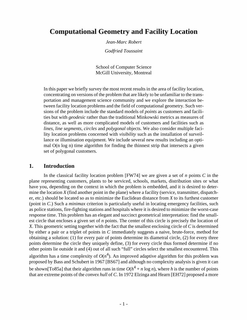
Fig. 2 Illustrating the geodesic convex hull (dashedlines) of the set of customers in Fig.1.

X

- 5 -

covered recently algorithms very simple to program that may turn out to be the most useful in prac-tice. In particular there exists an algorithm which runs in time O(n(1+t)) where t is a non-negativeinteger related to the shape complexity of P and t < n [To89]. The simplest of all sub-quadraticalgorithms however, requiring only a page of code, runs in time O(n(1+r)) where r is the numberof reflex vertices of P [KET90].

2.4 Geodesic Convex Hulls

In this sub-section we introduce the notion of the geodesic (also known in the literature asrelative) convex hull of a set of points (customers) lying in a simple polygon P. As we shall see inthe next section the geodesic convex hull is very useful in locating point-facilities using geodesicdistance criteria.

Let Q be a subset of P. Q is called geodesically convex provided that for every pair of pointsx,y ∈ Q, the geodesic path between x and y constrained to lie in P also lies in Q, i.e., GP(x,y/P) =GP(x,y/Q).

Let S be a set of customer-sites in P. The geodesic convex hull of S in P denoted by CHG(S/

P), is the intersection of all geodesically-convex sets containing S. Refer to Fig. 2 for an illustration.Alternately we may view the geodesic convex hull as the minimum-perimeter polygonal circuit thatcontains S and is constrained to lie in P.

3. Point-Facility Location

A general formulation of the problem considered in this section may be stated as follows:let C = c1,..., cn be a family of customers, X be the point-facility and f be the cost function given

by f(X) = g(w1d(X, c1),..., wnd(X, cn)) where d(X, ci) denotes the distance between the customer ciand the point-facility X, wi is the weight associated with customer ci and g is a norm function com-

bining all the weighted distances (usually the summation or the maximum function). The point-fa-cility problem is to determine an optimal solution, say X*, that minimizes the cost function f(X).Many aspects of this problem have been investigated in operations research with point-customersand they are summarized in the next subsection. Besides theses solutions, few attempts have beenmade to extend this problem to more complex models of customers. To remedy this situation, wewill present some extensions where the customers are lines, line segments or simple objects.

3.1 Points as customers

The point-facility location problem for point-customers with the Euclidean distance, de-fined as dE(p, q) =((xp - xq)2 + (yp - yq)2)1/2and the L∞-norm (i.e. the maximum function) is known

in the literature as the Euclidean 1-center problem. This problem has a very long history and wasposed originally in 1857 by Sylvester [Sy1857]. As mentioned in the introduction, Megiddo[Me83] presented an optimal linear time algorithm to solve the unweighted case. His solutionbased on the prune-and-search technique has been extended in [Dy86, Me84] to solve optimallythe weighted problem in any fixed dimension. With the L1-norm (i.e., the summation function) this

corresponds to the well known Fermat-Weber problem for which only heuristic solutions areknown [Ba84]. For the Manhattan distance, defined as dM(p, q) = xp - xq + yp - yq, the problem

- 4 -

tices of P. A simple polygon has a well defined interior and exterior. We will follow the conventionof including the interior of a polygon when referring to P. The vertices of P are either convex orreflex. A vertex is convex if its internal angle is less than 180° and reflex if it is greater than 180°.

A polygonal path is a simple path consisting of a sequence of line segments. If p is a po-lygonal path, then the length of p is the sum of the Euclidean lengths of all the line segments com-prising p. Given two points x and x’ in P the geodesic path between x and x’ denoted by GP(x,x’/P) is the minimum-length polygonal path (x=x1,x2,...,xk=x’). The length of the geodesic path is

called the geodesic distance and is denoted by dG(x,x’). Two fundamental properties of the geode-

sic path GP(x,x’/P) are that the path is unique and its vertices xi, i=2,3,...,k-1 are a subset of the

reflex vertices of P [Ch82], [LP84]. Chazelle [Ch82] and Lee and Preparata [LP84] independentlyobtained an elegant and simple algorithm for computing GP(x,x’/P) and dG(x,x’) optimally in lin-

ear time provided that P has already been triangulated. Since polygon triangulation plays a centralrole in many of these geodesic facility location algorithms we devote a short sub-section to thattopic next.

2.3 Triangulating Polygons

A triangulation of a simple polygon P containing n vertices is the decomposition of P witha set of n-3 internal diagonals (line segments [x,y] connecting pairs of vertices x,y of P such thatint[x,y] lies in int(P)) into n-2 triangles such that the diagonals intersect each other only at theirendpoints. Much work has been done to find efficient algorithms for triangulating simple polygonsand the interested reader is referred to [PS85] for an introduction to the subject and to [Ch90] fora review of the most recent work. Here we mention only the most important theoretical and prac-tical recent results. In the past fifteen years the theoretical complexity of triangulating polygons

has steadily decreased from O(n3) to O(n2) to O(n log n) to O(n log log n) and finally to O(n)[Ch90]. The fastest theoretical algorithms [Ch90] however appear to be very difficult to programand it is not clear just how useful they will be in practice. On the other hand there have been dis-

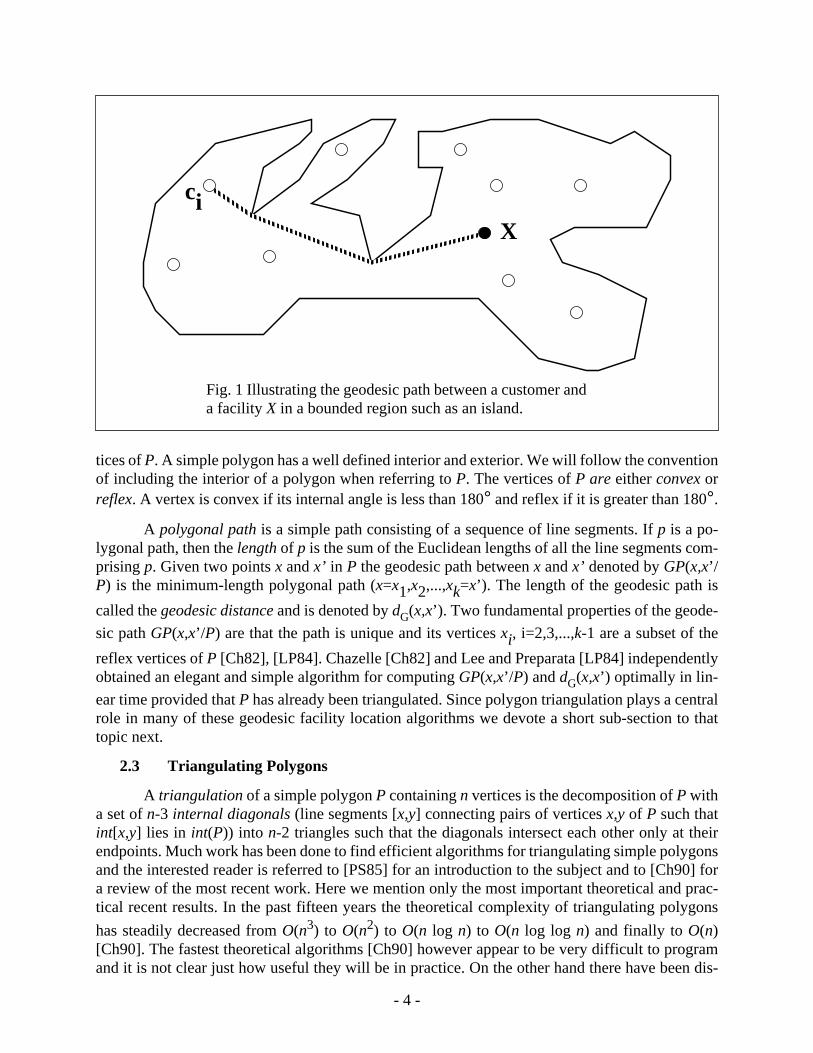
Fig. 1 Illustrating the geodesic path between a customer anda facility X in a bounded region such as an island.

ciX

- 3 -

computing such structures can be found.

2. Some Basic Computational Geometric Tools

2.1 Convex Hulls

One of the most useful structures in computational geometry is the convex hull of a set ofpoints C, i.e., the smallest convex set containing C [To85a]. In designing their facility location al-gorithm Bass and Schubert [BS67] used the fact that the smallest enclosing circle of a set of pointsC is determined only by points which are extreme on the convex hull of C. This fact together withan O(n log n) time algorithm which they propose for computing the convex hull of C, and a brute

force approach on the resulting extreme points leads to their complexity of O(h4 + n log n).

In practice we are often concerned with the average or expected time complexity of an al-gorithm. In 1978 Akl and Toussaint [AT78] proposed a sieve method they dubbed the throw-awayprinciple for computing convex hulls in linear expected time. The idea is to first throw away a“large” subset of the points with a very fast and simple O(n) time procedure and subsequently useany standard convex hull algorithm on the remaining set. This is accomplished by choosing an ap-propriate fixed number (say four or eight) of directions, searching for the extreme points in thesedirections, constructing the convex polygon determined by connecting the extreme points in aclockwise order, and finally discarding from further consideration the points of S that fall in theinterior of the resulting convex polygon. Akl and Toussaint [AT78] showed that for n points uni-formly distributed in the unit square an O(n log n) worst-case time algorithm could be made to runin O(n) expected time. Devroye and Toussaint [DT81] extended these results showing that for npoints randomly distributed in any non-degenerate rectangle R in the plane, according to any den-sity function f whatsoever, as long as f is zero outside R and bounded away from zero and infinityinside R, applying such a throw-away step to any algorithm will result in an overall expected com-plexity of O(n), even if the convex hull algorithm used after the throw-away step has a worst-case

complexity of O(n2). The FORTRAN code for a variant of this algorithm published by Bhatta-charya and Toussaint [BT83] appears to be the fastest in practice while using only 5n storage space.

2.2 Geodesic Paths

In the classical facility location problem discussed in the introduction it is tacitly assumedthat the space “between” the facility and the customers is not obstructed by obstacles of any sortwith the result that the shortest path between a customer ci and the point-facility X is the Euclidean

distance between ci and X. This is certainly a realistic situation if, for example, transportation is to

be carried out by helicopter or airplane. For ground transportation on the other hand it is often un-realistic as boundaries of countries may have to be respected or the region of interest may be anisland. In such situations it is more useful to model the customers as points in a polygonal regionP and to measure the distance between customer ci and the point-facility X by the geodesic distance

between ci and X, i.e., the length of the geodesic-path in P between ci and X. Figure 1 illustrates

the geodesic path between a facility X and a customer ci.

A polygon P is called a simple polygon provided that no point of the plane belongs to morethan two edges of P and the only points of the plane that belong to precisely two edges are the ver-

- 2 -

efficient (in the worst case) algorithm that runs in O(n2) time.

About four years later the computer science discipline of computational geometry was bornwith the work of Michael Shamos [Sh78]. Now a fifteen-year old explosive discipline it continuesto flourish at an exponentially increasing rate and make its presence felt in several areas not theleast of which is facility location. Several books have already appeared on the subject. An intro-ductory text by Preparata and Shamos [PS85] covers most of the early work. Mehlhorn [Me84]contains a subset of the material found in Preparata and Shamos along with a few different results.The combinatorial aspects of discrete and computational geometry as well as the prune-and-searchmethods useful in obtaining the fastest algorithms for many facility location problems are treatedin depth in the book by Edelsbrunner [Ed88]. The question of visibility, of great interest to locatingfacilities which consist of surveillance or illumination equipment, is notoriously absent from thethree texts mentioned above. However visibility is given a clear, excellent, and comprehensivetreatment in the recent book by O’Rourke [O’R87]. One of the most fundamental structures incomputational geometry is the Voronoi diagram and since the “birth” of computational geometrya score of variants on this structure have appeared. The book by Rolf Klein [Kl89] is entirely de-voted to this subject. There have also appeared five books which are collections of papers coveringalmost all aspects of computational geometry. The book edited by Preparata [Pr83] contains twelvepapers on early material. More recent results can be found in the two books edited by Toussaint[To85b], [To88a] and in the robotics-oriented collections edited by Schwartz et al., [SSH87] andSchwartz and Yap [SY87]. Journals are also starting to devote special issues to computational geo-metry such as The Visual Computer [To88], Pattern Recognition Letters [To91], and The Proceed-ings of the IEEE [To92].

The smallest enclosing circle (also minimal spanning circle) problem mentioned above aswell as many other facility location problems has benefited substantially from the developments incomputational geometry. Shamos [Sh78], Shamos and Hoey [SH75] and Preparata [Pr77] were the

first to discover O(n log n) time algorithms, a considerable improvement over the O(n2) solutionof Elzinga and Hearn [EH72]. The algorithms in [Sh78] and [SH75] have a step in which they com-pute the diameter of the set with an invalid diameter-algorithm and a counter-example to this di-ameter algorithm is given by Bhattacharya and Toussaint [BT85]. In spite of this default it is shownin [BT85] that the minimal spanning circle algorithm in [Sh78] always yields the correct solutionand two alternate O(n log n) time algorithms are also given there. Lee [Le80] proposed a similarO(n log n) time algorithm for computing the minimal spanning circle. Finally, Megiddo [Me83]found an optimal O(n) time algorithm for solving this problem.

In this paper we briefly survey the most recent results on facility location concentrating onversions of the problem that are probably unfamiliar to the transportation and management sciencecommunity. Such versions include the standard models of points as customers and facilities butwith geodesic rather than the traditional Minkowski metrics as measures of distance, as well asmore complicated models of customers and facilities such as lines, line segments, circles and po-lygonal objects. We also consider multiple facility location problems concerned with visibility suchas the installation of surveillance or lighting equipment. Since efficient algorithms for solvingmany of these problems depend heavily on some basic computational geometric structures we alsoprovide in the next section some pointers to the literature where the most efficient algorithms for

- 1 -

Computational Geometry and Facility LocationJean-Marc Robert

Godfried Toussaint

School of Computer ScienceMcGill University, Montreal

In this paper we briefly survey the most recent results in the area of facility location,concentrating on versions of the problem that are likely to be unfamiliar to the trans-portation and management science community and we explore the interaction be-tween facility location problems and the field of computational geometry. Such ver-sions of the problem include the standard models of points as customers and facili-ties but with geodesic rather than the traditional Minkowski metrics as measures ofdistance, as well as more complicated models of customers and facilities such aslines, line segments, circles and polygonal objects. We also consider multiple faci-lity location problems concerned with visibility such as the installation of surveil-lance or illumination equipment. We include several new results including an opti-mal O(n log n) time algorithm for finding the thinnest strip that intersects a givenset of polygonal customers.

1. Introduction

In the classical facility location problem [FW74] we are given a set of n points C in theplane representing customers, plants to be serviced, schools, markets, distribution sites or whathave you, depending on the context in which the problem is embedded, and it is desired to deter-mine the location X (find another point in the plane) where a facility (service, transmitter, dispatch-er, etc.) should be located so as to minimize the Euclidean distance from X to its furthest customer(point in C.) Such a minimax criterion is particularly useful in locating emergency facilities, suchas police stations, fire-fighting stations and hospitals where it is desired to minimize the worst-caseresponse time. This problem has an elegant and succinct geometrical interpretation: find the small-est circle that encloses a given set of n points. The center of this circle is precisely the location ofX. This geometric setting together with the fact that the smallest enclosing circle of C is determinedby either a pair or a triplet of points in C immediately suggests a naive, brute-force, method forobtaining a solution: (1) for every pair of points determine its diametral circle, (2) for every threepoints determine the circle they uniquely define, (3) for every circle thus formed determine if noother points lie outside it and (4) out of all such “full” circles select the smallest encountered. This

algorithm has a time complexity of O(n4). An improved adaptive algorithm for this problem wasproposed by Bass and Schubert in 1967 [BS67] and although no complexity analysis is given it can

be shown[To85a] that their algorithm runs in time O(h4 + n log n), where h is the number of pointsthat are extreme points of the convex hull of C. In 1972 Elzinga and Hearn [EH72] proposed a more