geophysical journal international - geodesy.geology.ohio

Geophysical Journal InternationalGeophys. J. Int. (2015) 203, 1773–1786 doi: 10.1093/gji/ggv392

GJI Gravity, geodesy and tides

GRACE time-variable gravity field recovery using an improvedenergy balance approach

Kun Shang,1 Junyi Guo,1 C.K. Shum,1,2 Chunli Dai1 and Jia Luo3

1Division of Geodetic Science, School of Earth Sciences, The Ohio State University, 125 S. Oval Mall, Columbus, OH 43210, USA. E-mail: [email protected] of Geodesy & Geophysics, Chinese Academy of Sciences, Wuhan, China3School of Geodesy and Geomatics, Wuhan University, 129 Luoyu Road, Wuhan 430079, China

Accepted 2015 September 14. Received 2015 September 12; in original form 2015 March 19

S U M M A R YA new approach based on energy conservation principle for satellite gravimetry mission hasbeen developed and yields more accurate estimation of in situ geopotential difference observ-ables using K-band ranging (KBR) measurements from the Gravity Recovery and ClimateExperiment (GRACE) twin-satellite mission. This new approach preserves more gravity in-formation sensed by KBR range-rate measurements and reduces orbit error as compared toprevious energy balance methods. Results from analysis of 11 yr of GRACE data indicatedthat the resulting geopotential difference estimates agree well with predicted values from of-ficial Level 2 solutions: with much higher correlation at 0.9, as compared to 0.5–0.8 reportedby previous published energy balance studies. We demonstrate that our approach produced acomparable time-variable gravity solution with the Level 2 solutions. The regional GRACEtemporal gravity solutions over Greenland reveals that a substantially higher temporal resolu-tion is achievable at 10-d sampling as compared to the official monthly solutions, but withoutthe compromise of spatial resolution, nor the need to use regularization or post-processing.

Key words: Satellite geodesy; Geopotential theory; Time variable gravity.

1 I N T RO D U C T I O N

Launched in March 2002, the Gravity Recovery and Climate Ex-periment (GRACE) mission (Tapley et al. 2004a) has been map-ping Earth’s time-variable gravity field for more than a decade andachieving remarkable and even transformative scientific advances(Cazenave & Chen 2010). From the data collected by the K-bandranging (KBR) low–low satellite-to-satellite tracking (SST) as wellas the high-low GPS tracking, monthly mean gravity field mod-els, known as the Level-2 data products, have been routinely esti-mated by the University of Texas Center for Space Research (CSR),GeoForschungsZentrum (GFZ) Helmholtz-Centre Potsdam Ger-man Research Centre for Geosciences, NASA’s Jet Propulsion Lab-oratory (JPL) and others. The estimation approach used by the abovethree agencies and others (e.g. Luthcke et al. 2006; Bruinsma et al.2010) to generate these solutions is the so-called dynamic methodbased on the dynamic orbit determination and geophysical parame-ter recovery principle (Tapley et al. 2004b). Dynamic method treatsboth KBR and GPS tracking as observations but with differentweights, and simultaneously estimates for the state parameters in-cluding the gravity coefficients, orbits and others in a least-squaressolution. Because of the non-linear relationship between observa-tions and the state parameters, linearization of both the dynamicalequation of motion and the observation-state equations are requiredduring the estimation process. Besides the conventional dynamic

method, various alternative approaches have also been proposedand implemented, such as mascon approach (Rowlands et al. 2005,2010), short-arc approach (Mayer-Gurr et al. 2007; Kurtenbachet al. 2009), celestial mechanics approach (Meyer et al. 2012), ac-celeration approach (Ditmar & van Eck van der Sluijs 2004; Chenet al. 2008; Liu et al. 2010) and the energy balance approach (Jekeli1999; Han et al. 2006; Ramillien et al. 2011; Tangdamrongsub et al.2012). The last approach is the focus of this paper.

Energy balance approach, also known as energy integral ap-proach, can be traced back to the 1960s (e.g. Bjerhammar 1969), inthe early era of satellite geodesy. The basic idea of this approach isto explore the possibility of applying the principle of energy conser-vation, that is the constant sum of kinematic energy and potentialenergy, to the SST data for direct measuring of Earth’s gravityfield. The concept was investigated again by Jekeli (1999) at theonset of the Decade of Geopotential Missions, and he developedthe first practical formulation to explicitly express the relationshipbetween geopotential and satellite data in inertial frame (later calledthe energy equation), with conceived application for the forthcom-ing satellite gravimetry missions, Challenging Minisatellite Pay-load (CHAMP) and GRACE. Shortly after, Visser et al. (2003)similarly derived the energy equation but in the Earth-fixed frame.Since then, a renewed interest of using energy balance approach toestimate Earth’s static and time-variable gravity field was arousedduring the last decade, especially for application using the data from

C© The Authors 2015. Published by Oxford University Press on behalf of The Royal Astronomical Society. 1773

at Ohio State U

niversity Libraries on D

ecember 20, 2016

http://gji.oxfordjournals.org/D

ownloaded from

mailto:[email protected]

http://gji.oxfordjournals.org/

1774 K. Shang et al.

Earth satellite gravimetry missions, such as CHAMP (e.g. Han et al.2002; Gerlach et al. 2003; Badura et al. 2006), GRACE (e.g. Hanet al. 2006; Ramillien et al. 2011; Tangdamrongsub et al. 2012) andGravity Field and Steady-State Ocean Circulation Explorer (GOCE;e.g. Pail et al. 2011).

One of the major advantages of energy balance approach is thatit can be utilized to estimate the in situ geopotential observables(for a single satellite) or geopotential difference observables (for apair of satellites), which means that the geopotential or geopoten-tial differences can be computed at the satellite altitude, and thenused to solve for the Earth’s gravity field. Similarly, accelerationapproach (Ditmar & van Eck van der Sluijs 2004) can also generatein situ observables, but in the form of acceleration. In contrast, con-ventional dynamic method normally cannot provide this kind of insitu observables, where the geometric measurements, that is KBRand GPS tracking, have to be applied to directly solve gravity field,that is Stokes coefficients. The in situ geopotential observables,as a quantity with explicit geophysical interpretation, can serve asan intermediate product between the satellite measurements andfinal gravity solutions, since the estimation procedure is more ef-ficient because of the linear relationship between the observablesand gravity coefficients. More importantly, the in situ geopoten-tial difference observables would greatly benefit the time-variablegravity recovery missions, such as GRACE, since the epoch-wiseobservables can support flexible spatial and temporal resolutions,leading to regional solutions with possibly retrieving more localgravity information (Han et al. 2005; Schmidt et al. 2006, 2008;Tangdamrongsub et al. 2012).

However, appropriate application of energy balance approachon GRACE-type mission data for highly accurate geopotential es-timation is still a demanding task. One of the most challengingproblems is how to efficiently extract the gravity signal sensed bythe essential measurements from SST, that is KBR range-rate mea-surements, which the energy equation does not explicitly contain.Previous researchers attempted to adjust range-rate and orbit datasimultaneously via a non-linear least-squares estimation with eitherfixed constraints (Han et al. 2006) or via stochastic constraints(Tangdamrongsub et al. 2012). The use of constrained least-squares adjustment, though straightforward, is still a compromisebetween the very high-precision range-rate data and the relative low-precision orbit data, which may tend to distort the estimation of insitu geopotential observables caused by errors including orbit error.The orbit error, inherited from the chosen reference orbit, wouldcontaminate the resulting gravity estimation especially at the low-frequency band (Ditmar et al. 2012). In addition, our recent study(Guo et al. 2015) has demonstrated that the previous formulationof the energy equation may contain a non-negligible approxima-tion, which could sometimes overwhelm the time-variable gravitysignal also at the low-frequency band. These issues limit the appli-cation of the earlier developed in situ geopotential differences onlyto regional gravity analysis, that is at the high-frequency band, andarguably over regions with large temporal gravity field signals. Asa result, large-scale gravity field inversion, including global grav-ity solution, has not been fully exploited based on previous energyapproach.

The primary purpose of this study is to overcome these limitationsby employing an improved energy balance approach to obtain a moreaccurate estimation of in situ geopotential difference observables,with the aim to preserve both the low- and high-frequency grav-ity signal and consequently yield a full scale, that is both regionaland global, gravity inversion. To achieve this goal, we develop anovel formulation, called the alignment equation, to incorporate

range-rate observations into energy equation, together with amethod to reconstruct the related reference orbit. In addition, amore rigorous formulation of energy equation (Guo et al. 2015)is applied to model the in situ geopotential difference observables,which is requisite for the reduction of the GRACE measurementsfor gravity field inversion.

The outline of this paper is as follows: Section 2 starts with abrief description of the general idea of energy balance formalism,followed by a detailed description of the methodology about ourimproved approach. Section 3 presents the numerical results usingthe new energy approach, on the validation of the accuracy of theresulting improved in situ geopotential difference observables, andon using the observables to demonstrate monthly and 10-d temporalgravity recovery. Finally, conclusions and discussions are summa-rized in Section 4.

2 M E T H O D O L O G Y

The orbit data, both positions and velocities, are dominated bythe gravitational perturbations and other forces, and thus can beregarded as observations and used for gravity recovery after properreduction of other forces, which is the basic concept of the energybalance approach. The energy equation, a mathematical expressionof this concept, can be formulated in Earth-centred inertial frame(Jekeli 1999) for a single satellite as

V = 1

2|r|2 +

∫ t

t0

∂V

∂tdt −

∫ t

t0

f · rdt − E0, (1)

where V is the total gravitational potential (for unit mass), r (implicitin V) and r are the orbit position and velocity in inertial frame, f isthe non-conservative force,

∫ tt0

(∂V

/∂t

)dt is the so-called potential

rotation term, and E0 is an integral constant. The total gravitationalpotential V can be decomposed into two parts V = VE + VR, whereVE is the geopotential, including the Earth’s mean, secular, seasonaland other variable components, and VR is the residual gravitationalpotential, mostly from the high-frequency (e.g. semi-diurnal anddiurnal) variable geopotential, such as tides. If we assume the resid-ual gravitational potential VR can be reduced or corrected using apriori model, and also non-conservative force f can be measured byan on-board accelerometer, we arrive at the complete formulationof energy equation for estimating geopotential VE, from a singlesatellite, such as CHAMP, which can be expressed as

V E = 1

2|r|2 +

∫ t

t0

∂V

∂tdt −

∫ t

t0

f · rdt − V R − E0. (2)

And for estimating geopotential difference from a pair of satel-lites, such as GRACE, the formulation is simply the subtractionbetween the equations of two single satellites:

V E12 = V E

2 − V E1

= 1

2|r12|2 + r1 · r12 +

∫ t

t0

∂V12

∂tdt

−∫ t

t0

(f2 · r2 − f1 · r1) dt − V R12 − E0

12, (3)

where the subscripts represent the two satellites (‘1’, ‘2’) and theirdifference (‘12’). It is worth mentioning that the orbit data (r and r)in both formulations are normally regarded as observables, whichare usually from a precomputed reference orbit using high-low GPStracking data.

at Ohio State U


ecember 20, 2016


ownloaded from


GRACE improved energy balance approach 1775

2.1 A novel method to incorporate range-ratemeasurements into energy equation

Application of energy balance approach on GRACE-type mission ismuch more challenging than CHAMP-type mission because energyeq. (3) is unable to explicitly contain the tracking measurementsfrom the low–low SST system, that is range-rate measurementsfrom KBR system in the case of GRACE. Previous studies of en-ergy balance approach usually treat range-rate measurements as akind of redundancy observation, and adjust them simultaneouslywith orbit data along the orbit, by a non-linear least-squares esti-mation, where the energy equation is treated as either a fixed (Hanet al. 2006) or stochastic (Tangdamrongsub et al. 2012) constraint.The estimates would be the six intersatellite orbit state componentswith some other empirical parameters. However, we know that theuncertainty of GRACE orbits is around 1–2 cm in positions and10–20 µm s–1 in velocities (only for dynamic orbit; for kinematicorbit the uncertainty in velocities is even worse; Kang et al. 2006),whereas the range-rate measurements have a much lower uncer-tainty of about 0.2 µm s–1 (Loomis et al. 2012) at high-frequencyband. The use of constrained least-squares adjustment in energybalance approach may be able to extract some information fromrange-rate measurement, but it’s still a compromise between high-precision data and low-precision data, as the (unknown) systematicerror, for example from orbit errors, would inevitably affect thesolved parameters, and subsequently bias the estimation of geopo-tential difference observables.

Therefore, in this study we present a new, alternative method toadjust intersatellite orbit state components using range-rate mea-surements. The motivation is based on a simple fact, which is thatthe range-rate measurements cannot be sensitive to all the intersatel-lite orbit components. Previous study by Rowlands et al. (2002) hasalready shown that, among all the intersatellite components, the rel-ative velocity pitch is the most sensitive to range-rate measurements,and also one of the most important components for gravity recov-ery (Luthcke et al. 2006). The other two important components arerelative velocity magnitude and relative position pitch, but these aremuch less sensitive to range-rate measurements compared to rela-tive velocity pitch. Based on this fact, we aim to develop a methodto use range-rate measurements to only adjust the most sensitivecomponent, that is relative velocity pitch, and adopt the other lesssensitive or insensitive components to be provided by the referenceorbits.

The method is accomplished through a simple equation as fol-lows:

rρ

12 = ρr12

|r12| +√

|r12|2 − ρ2r12 × r12 × r12

|r12 × r12 × r12| (4)

which is referred to as alignment equation throughout this pa-per. Here ρ represents the range-rate measurement, r12 and r12

are the relative position and velocity vector from reference orbit,r12 × r12 × r12 is the vector triple product between them, and rρ

12

represents the new relative velocity vector. As we can see, the newrelative velocity vector rρ

12 would be equal to the original vec-tor r12 if there were no additional range-rate observation, that isρ = r12 · r12

/|r12|. In that case, the alignment equation would de-grade to an identical equation, which represents an exact geometricrelationship between relative velocity direction vector and range-rate measurement. That means the alignment equation itself doesnot contain any approximation.

Once we have an independent and more accurate measuring ofrelative range-rate, such as the case of GRACE, then the new relative

Figure 1. Geometric configuration of GRACE constellation and its relation-ship with alignment equation. (a) The absolute position and velocity vectorfor GRACE satellites with respect to the Earth’s centre of mass (CM). (b)The intersatellite components of position and velocity vector and the de-composition of velocity vector, illustrating the derivation of the alignmentequation.

velocity vector rρ

12 would become more accurate compared to theoriginal vector r12 because the pitch angle of relative velocity vectorhas been constrained by, or we can say, aligned to the range-rate.The term ‘alignment’ actually means the relative velocity pitch,the most sensitive intersatellite parameter to range-rate and mostimportant parameter for gravity recovery, has been aligned to therange-rate measurement through the equation. The reason can befurther explained as follows.

The alignment equation decomposes relative velocity vectors intotwo components. Fig. 1 illustrates such decomposition by show-ing the simple geometric configuration of GRACE constellation,where Fig. 1(a) shows the absolute position and velocity vector forGRACE satellites with respect to the Earth’s centre of mass (CM),and Fig. 1(b) shows the decomposition of velocity vector. As shownin Fig. 1(b), the intersatellite velocity is decomposed into two or-thogonal directions. One is along the line-of-sight (LOS) direction,where unit vector is n1 = r12

/|r12|, and the correspondent projec-tion is ρ. The other is orthogonal to the LOS direction and is inthe plane containing relative position vector and velocity vector,where the unit vector is n2 = (r12 × r12 × r12)

/|r12 × r12 × r12|,with the correspondent projection of

√|r12|2 − ρ2 in order to main-

tain the same magnitude of the intersatellite velocity.Again, our goal here is to use high accurate measurement, that

is the range-rate measured by the KBR, to adjust the most sensitiveintersatellite parameter, that is the relative velocity pitch. In anotherwords, range-rate should be used to replace the relative velocitypitch component and form a new ‘pitch-free’ relative velocity vec-tor. That is exactly what the alignment equation represents. Underthe decomposition as eq. (4), the computation of rρ

12 only requiresfour intersatellite quantities, which are range-rate ρ, relative veloc-ity magnitude |r12|, LOS direction unit vector n1, and direction unitvector n2 that is always perpendicular to n1 and in the plane of in-tersatellite position and velocity. Among the four quantities, two ofthem, ρ and n1, are totally independent of the velocity component(as well as the position magnitude), and |r12| is only dependent onthe velocity magnitude. The last one, unit vector n2, does rely onthe velocity direction, but only the yaw angle. n2 does not dependon the relative velocity pitch at all simply because it is always per-pendicular to n1 in the plane of intersatellite position and velocity.Therefore, by using the alignment equation, the components thatare needed from reference orbit are only relative velocity magni-tude, relative position direction and relative velocity yaw, but notrelative velocity pitch. The effect of relative velocity pitch from lessaccurate reference orbit is thus totally eliminated. The only contri-bution of the resulting relative velocity pitch is from range-rate, and

at Ohio State U


ecember 20, 2016


ownloaded from



therefore the most sensitive component to intersatellite observation,has been fully constrained by range-rate measurement through thealignment equation.

After applying the alignment equation, the new relative velocityvector rρ

12, would subsequently be used as the input of energy eq. (3).In the next step, we expect to determine geopotential differenceobservables solely from range-rate measurements, and meanwhileminimize the direct effect from the reference orbit to the estimates,which will be discussed in the next subsection.

2.2 Reconstruction of the reference orbit

The reference orbit is another critical input to the energy eq. (3)in addition to the range-rate measurements. Generally there existthree different choices of reference orbits, namely the kinematic,reduced-dynamic or dynamic orbit, for the case of GRACE. Sincerange-rate should dominate the time-variable gravity information,the geopotential difference estimates do not rely much on the choiceof the reference orbit. Therefore, it is possible to choose dynamicor reduced-dynamic orbit as the reference orbit for GRACE gravityfield recovery, as long as the range-rate measurements are appro-priately used to correct or adjust the orbit data. In practice, variousreference orbit data have indeed been implemented for GRACE realdata analysis (Han et al. 2006; Tangdamrongsub et al. 2012).

In this study, we choose to adopt a pure dynamic orbit as the ref-erence orbit. However instead of computing a dynamic orbit directlyfrom GPS observations, we use an alternative method to reconstructthe pure dynamic orbit from existing orbit data products. The similartechnique has been used for previous studies on GRACE (Liu et al.2010) and GOCE (Yi 2012). The idea is to treat the available orbitcoordinates as pseudo observations, and estimate a pure dynamicorbit by fitting the orbit coordinates with respect to a completereference model, via least-squares adjustment. Meanwhile, the ac-celerometer data are also simultaneously calibrated with respect tothe pure dynamic orbit. The reference models we used in this studyare identical to the models used by GFZ for solving the officialGRACE Level-2 (L2) product Release 05 (RL05; Biancale & Bode2006; Petit & Luzum 2010; Dahle et al. 2012; Mayer-Gurr et al.2012). We also adopt a similar strategy for calibrating accelerometerdata, which is to estimate daily biases, and monthly scale factors.The accelerometer data from GRACE Level 1B (L1B) ACC1Bproduct, together with orientation data from L1B SCA1B product,are used to model the non-gravitational forces. The GRACE L1Bdata can be downloaded via http://podaac.jpl.nasa.gov/GRACE.

As for the input of the reconstruction of the pure dynamic orbit,we have tested three different highly accurate scientific orbit prod-ucts from independent institutes, which are kinematic orbit prod-uct from National Central University, Taiwan (T. Tseng, personalcommunication, 2014), kinematic orbit product from Universityof Bern (A. Jaggi, personal communication, 2014), and reduced-dynamic orbit from JPL, that is the GRACE L1B GNV1B product.We found the difference between the resulting reconstructed puredynamic orbits using these orbit products negligible. For exampleof one satellite on 2009 January 25, the direct orbit position dif-ference between two products from University of Bern and JPL isabout 2.48 cm (rms), and after reconstruction, the resulting orbitdifference is reduced to 0.76 cm (rms). More importantly, the sub-sequent geopotential difference observables are also not sensitiveto the input orbit product because of the reconstruction process. Forthe resulting geopotential differences on the same day, the differ-ence between the two estimates based on the two orbit products is

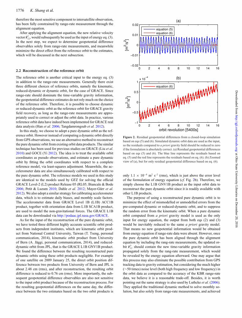
Figure 2. Residual geopotential differences from a closed-loop simulationbased on eqs (5) and (6). Simulated dynamic orbit data are used as the input,so the residuals compared to a priori gravity field should be reduced to zeroif the formulation is absolutely correct. (a) Residual geopotential differencesbased on eqs (5) and (6). The blue line represents the residuals based oneq. (5) and the red line represents the residuals based on eq. (6). (b) Zoomedview of (a), but for only residual geopotential difference based on eq. (6).

only 1.1 × 10−4 m2 s–2 (rms), which is just above the error levelof the formulation of energy equation (cf. Fig. 2b). Therefore, wesimply choose the L1B GNV1B product as the input orbit data toreconstruct the pure dynamic orbit since it is readily available withother L1B products.

The purpose of using a reconstructed pure dynamic orbit is tominimize the effect of mismodelled or unmodelled errors from thepre-computed dynamic or reduced-dynamic orbit, and to suppressthe random error from the kinematic orbit. When a pure dynamicorbit computed from a priori gravity model is used as the onlyinput for energy equation, the output from both eqs (2) and (3)would be inevitably reduced to the same a priori gravity model.That means no new geopotential information would be obtainedfrom energy equation if range-rate data were absent. However, oncethe pure dynamic orbit has been aligned through the alignmentequation by including the rang-rate measurements, the updated or-bit rρ

12 should contain the new time-variable gravity informationpropagated solely from the rang-rate measurement, which wouldbe revealed by the energy equation afterward. One may argue thatthis process may also eliminate the possible contribution from GPStracking data to gravity estimation, but considering the much higher(∼50 times) noise level (both high frequency and low frequency) inthe orbit data as compared to the accuracy of the KBR range-ratedata, we believe it is a reasonable trade-off. Besides, it is worthpointing out the same strategy is also used by Luthcke et al. (2006).They applied the traditional dynamic method to solve monthly so-lution, but also solely from range-rate measurements, and achieved

at Ohio State U


ecember 20, 2016


ownloaded from

http://podaac.jpl.nasa.gov/GRACE



comparable GRACE solutions as compared to the official GRACELevel 2 data products.

2.3 Reformulation of energy equation

When energy eq. (3) is applied to compute the geopotential dif-ference, all the quantities and terms on the right-hand side canbe computed from data or based on reference models, except oneterm,

∫ tt0

(∂V

/∂t

)dt , the so-called ‘potential rotation term’. In the

previous formulation developed by Jekeli (1999)

V E ≈ 1

2|r|2 − ω (x y − yx) −

∫ t

t0

f · rdt − V R − E0, (5)

the potential rotation term was approximated as∫ t

t0

(∂V

/∂t

)dt ≈

−ω (x y − yx), where x and y represent the first and second com-ponent of the position vector, and ω is the nominal mean Earth’sangular velocity. However, Guo et al. (2015) have already demon-strated via simulation that this approximation of potential rotationterm exceeds the precision of GRACE observation, and suggesteda more accurate formulation of energy equation as follows:

V E ≈ 1

2|r|2 − w · (r × r) −

∫ t

t0

a · (r − w × r) dt − E0, (6)

where a = ∇V R + f is the acceleration of both residual geopoten-tial acceleration and non-conservative acceleration, and w is Earth’sangular velocity of Earth-fixed frame relative to the inertial frame,with coordinates in the inertial frame. The third term of the right-hand sides can be numerically integrated. The detailed derivationcan be found in the Appendix, where we also demonstrate the equiv-alence of the energy equations in both inertial frame and Earth-fixedframe (Jaggi et al. 2008; Wang et al. 2012). Thus there is no differ-ence no matter in which frame the energy equation is used for theenergy balance method.

The Appendix also shows that two approximations are includedin eq. (6). One is to assume VE to be static during the integral limitsfrom t0 to t, which is consistent with the normal GRACE conven-tion that is estimating a mean gravity field during a certain timeinterval. The other one is to assume the rates of Earth’s angular ve-locity vector is zero, that is w = 0, which is negligible compared tomeasurement noise level of GRACE (Guo et al. 2015). In contrast,eq. (5) contains too many rough approximations that would pollutethe signal level of GRACE. In order to check the accuracy of thetwo formulations, a closed-loop validation is performed. We firstsimulate pure dynamic orbits for two satellites as the input to theenergy equation. As we mentioned in the last subsection, using apure dynamic orbit data as the input of energy equation should re-duce the estimates to the a priori gravity field. If we define residualgeopotential difference observables as: �V E

12 = V E12 − V E apriori

12 ,that is the difference between the estimated values using energyequation and the predicted values using the a priori gravity model,then theoretically the residual should be reduced to zero, and there-fore the non-zero residual would reveal the approximation level foreach formulation of energy equation.

The residuals based on eqs (5) and (6) are presented in Fig. 2,for an integration period of 1 d. Fig. 2(a) shows the residuals basedon both equations, and we can see that the one based on eq. (6) isreduced to almost zero, but the one based on eq. (5) contains a rela-tive large non-zero residual with a dominate 2 cycle-per-revolution(CPR) error, which is caused by the approximation primarily fromthe potential rotational term. A zoomed-in view of the error fromeq. (6) is presented in Fig. 2(b), and the peak-to-peak amplitude

is less than 1×10−4 m2 s–2, which is definitely negligible for cur-rent GRACE measurement accuracy and probably also for GRACEfollow-on measurement accuracy in the future (Loomis et al. 2012).More detailed numerical comparison can be found in Guo et al.(2015). The error level based on eq. (5) is about 0.02 m2 s–2 frompeak to peak, which is larger than the signal level from the time-variable gravity field (see next Section on the resulting geopotentialdifference estimates using real data). All these errors caused by theapproximation would surely corrupt the geopotential difference es-timates. It seems that the dominant errors have the frequency closeto 2 CPR, which might be removed by an additional 2 CPR param-eters (Han et al. 2006; Tangdamrongsub et al. 2012) or even moreparameters (Ramillien et al. 2011), but actually the errors containmuch more high-frequency constituents (e.g. from ocean tides),which empirical parameters cannot fully absorb these errors. Alsowe know that 2 and higher CPR empirical parameters would heavilycontaminate gravity signal, especially the zonal geopotential coef-ficients. The studies based on traditional orbit dynamic approachalso indicate that the empirical parameterization should be no morethan 1 CPR (Tapley et al. 2004a) or even less parameters (Luthckeet al. 2006), which is for the purpose to mitigate the systematicerror of range-rate data, and also to better retain the time-variablegeopotential signal. Therefore, we conclude that in order to fullyexploit the precision of GRACE data, it is requisite to choose eq. (6)as the practical formulation of energy equation.

3 R E S U LT S A N D A NA LY S I S

3.1 Geopotential difference estimates

After the reduction of non-conservative acceleration and other tidalpotential terms, each geometric observation from GRACE can bedirectly linked to a geophysical quantity, that is geopotential differ-ence between the two positions of the twin satellites, and thereforeenergy balance approach could provide a unique ability to extendour conventional knowledge about both data processing and resultsinterpretation of GRACE. The geopotential difference estimates areable to directly sense the gravity information, without losing anyhigh-frequency resolution, since each estimate is computed straightfrom range-rate measurement for each epoch. Because of that, thegeopotential difference estimates could not only be used for bothglobal and regional gravity recovery but also be regarded as anin situ gravity representation without downward continuation (Hanet al. 2006). Therefore, an accurate estimation of geopotential dif-ference observables is the key issue for energy balance approachand is the most critical step for the subsequent temporal gravityinversion.

Using the methods described in the previous section, geopotentialdifferences are estimated for each day from 2003 to 2013. All theinput data are from GRACE L1B data products, including GNV1Borbit data that are used to reconstruct the pure dynamic orbit andestimate the daily accelerometer calibration parameters. Range-ratedata from KBR1B product are then included to correct the velocitycomponents of the reconstructed orbit via the alignment eq. (4).Next, energy eq. (3) is applied according to the formulation ofeq. (6), to compute the geopotential difference observables.

The accelerometer measures the non-conservative force in threeorthogonal directions of the Science Reference Frame (SRF), whichcan be transformed into inertial frame using the quaternions fromthe SCA1B product measured by the Star Camera Assembly. Ap-proximately, X direction is along roll axis in the anti-flight and

at Ohio State U


ecember 20, 2016


ownloaded from



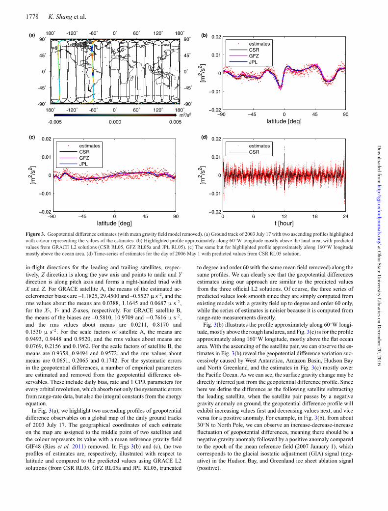
Figure 3. Geopotential difference estimates (with mean gravity field model removed). (a) Ground track of 2003 July 17 with two ascending profiles highlightedwith colour representing the values of the estimates. (b) Highlighted profile approximately along 60◦W longitude mostly above the land area, with predictedvalues from GRACE L2 solutions (CSR RL05, GFZ RL05a and JPL RL05). (c) The same but for highlighted profile approximately along 160◦W longitudemostly above the ocean area. (d) Time-series of estimates for the day of 2006 May 1 with predicted values from CSR RL05 solution.

in-flight directions for the leading and trailing satellites, respec-tively, Z direction is along the yaw axis and points to nadir and Ydirection is along pitch axis and forms a right-handed triad withX and Z. For GRACE satellite A, the means of the estimated ac-celerometer biases are –1.1825, 29.4500 and –0.5527 µ s–2, and therms values about the means are 0.0388, 1.1645 and 0.0687 µ s–2,for the X-, Y- and Z-axes, respectively. For GRACE satellite B,the means of the biases are –0.5810, 10.9709 and −0.7616 µ s–2,and the rms values about means are 0.0211, 0.8170 and0.1530 µ s–2. For the scale factors of satellite A, the means are0.9493, 0.9448 and 0.9520, and the rms values about means are0.0769, 0.2156 and 0.1962. For the scale factors of satellite B, themeans are 0.9358, 0.9494 and 0.9572, and the rms values aboutmeans are 0.0651, 0.2065 and 0.1742. For the systematic errorsin the geopotential differences, a number of empirical parametersare estimated and removed from the geopotential difference ob-servables. These include daily bias, rate and 1 CPR parameters forevery orbital revolution, which absorb not only the systematic errorsfrom range-rate data, but also the integral constants from the energyequation.

In Fig. 3(a), we highlight two ascending profiles of geopotentialdifference observables on a global map of the daily ground tracksof 2003 July 17. The geographical coordinates of each estimateon the map are assigned to the middle point of two satellites andthe colour represents its value with a mean reference gravity fieldGIF48 (Ries et al. 2011) removed. In Figs 3(b) and (c), the twoprofiles of estimates are, respectively, illustrated with respect tolatitude and compared to the predicted values using GRACE L2solutions (from CSR RL05, GFZ RL05a and JPL RL05, truncated

to degree and order 60 with the same mean field removed) along thesame profiles. We can clearly see that the geopotential differencesestimates using our approach are similar to the predicted valuesfrom the three official L2 solutions. Of course, the three series ofpredicted values look smooth since they are simply computed fromexisting models with a gravity field up to degree and order 60 only,while the series of estimates is noisier because it is computed fromrange-rate measurements directly.

Fig. 3(b) illustrates the profile approximately along 60◦W longi-tude, mostly above the rough land area, and Fig. 3(c) is for the profileapproximately along 160◦W longitude, mostly above the flat oceanarea. With the ascending of the satellite pair, we can observe the es-timates in Fig. 3(b) reveal the geopotential difference variation suc-cessively caused by West Antarctica, Amazon Basin, Hudson Bayand North Greenland, and the estimates in Fig. 3(c) mostly coverthe Pacific Ocean. As we can see, the surface gravity change may bedirectly inferred just from the geopotential difference profile. Sincehere we define the difference as the following satellite subtractingthe leading satellite, when the satellite pair passes by a negativegravity anomaly on ground, the geopotential difference profile willexhibit increasing values first and decreasing values next, and viceversa for a positive anomaly. For example, in Fig. 3(b), from about30◦N to North Pole, we can observe an increase-decrease-increasefluctuation of geopotential differences, meaning there should be anegative gravity anomaly followed by a positive anomaly comparedto the epoch of the mean reference field (2007 January 1), whichcorresponds to the glacial isostatic adjustment (GIA) signal (neg-ative) in the Hudson Bay, and Greenland ice sheet ablation signal(positive).

at Ohio State U


ecember 20, 2016


ownloaded from



In Fig. 3(d), we show a profile as a time-series for a differentday (2006 May 1) with predicted time-series from CSR L2 RL05solution for comparison. Again, the time-series of the estimatesseems very close to the predicted values from CSR solution. Inorder to compare with previous study, we adopt the same methodfrom Han et al. (2006) to compute the correlation coefficient ofthe time-series between the (smoothed) estimates and the predictedvalues. The resulting correlation coefficient is about 0.91 for thatparticular day. The rms of the difference between the (smoothed)estimates and the predicted values is about 8.4 × 10−4 m2 s–2,and for comparison, the rms of the values themselves is about0.002 m2 s–2. As for all the estimates from 2003 to 2013, the averagevalue of the daily correlation coefficients is over 0.9, which is muchhigher than correlations of 0.5–0.8 reported in previous study byHan et al. (2006).

3.2 Global gravity solutions using geopotential differenceobservables

As an in situ observation type, geopotential differences have beenwidely used for gravity recovery, especially for regional gravityrecovery. However, the global gravity recovery using geopotentialdifferences is not commonly used, even if it is more straightforwardbecause of the linear relationship between geopotential differencesand Stokes coefficients. In this subsection, we explored the possibil-ity of global gravity recovery based on the geopotential differenceestimates from our improved approach.

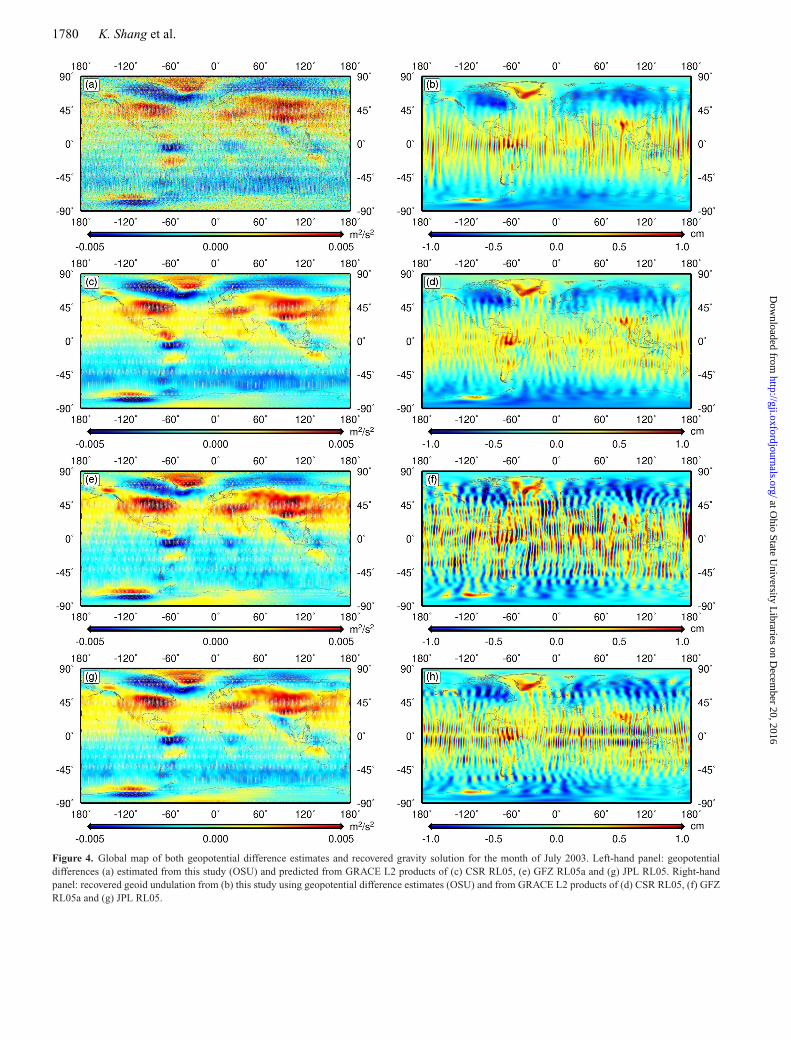
Similar to the convention of official GRACE L2 product, wealso produce monthly mean solutions for each calendar month.First, similar to Fig. 3(a), we plot all the accumulated geopotentialdifference estimates for an example month of July 2003 on the globalmap in Fig. 4(a). The data from descending passes are presented withan additional minus sign so they would not look opposite to the datafrom ascending passes over the same region of the global map. FromFig. 4(a), we can see that some regions with large gravity variationare manifested in the global map, including not only the highlightedregions in Fig. 3(a) but also some other regions like Alaska (glaciermelting), Congo Basin (wet season), and Scandinavia (GIA).

For comparison, the other three figures in the left-hand column ofFig. 4 show the predicted values at the same geographical locationfrom three GRACE L2 solutions completed to spherical harmonicdegree and order 60 (Fig. 4c for CSR RL05, Fig. 4e for GFZ RL05aand Fig. 4g for JPL RL05). The most significant discrepancy be-tween Fig. 4(a) and other three figures in the left (Figs 4c, e andg) is that Fig. 4(a) apparently contains measurement noise whichis inherited from each range-rate measurement, while other threefigures are only predicted from a truncated gravity field model withresolution of up to degree 60. That shows the key contributionof using energy balance approach, that is directly connecting thegeometry measurements (range-rate) to the geophysical quantities(geopotential difference). Therefore, even though we plot the wholemonth estimates in the same global map, Fig. 4(a) still preserve thein situ geopotential change for each epoch within a month, that issubmonthly information, but Figs 4(c), (e) and (g) can only showthe predicted values from a monthly mean (static) gravity field.

Next, we use the accumulated estimates to produce a monthlyglobal solution. The relation of geopotential difference V E

12 andStokes coefficients (Cnm and Snm) can be expressed as

V E12 = G M

R

nmax∑n=2

n∑m=0

(αnmCnm + βnm Snm

), (7)

where GM is the geocentric gravitational constant and R is Earth’sradius, n and m are degree and order, respectively, and nmax is themaximum degree, that is 60 in this study. Here we exclude degree 0and degree 1 coefficients, as GRACE range rate measurements areinsensitive to these parameters. The coefficients αnm and βnm aredefined as⎧⎨⎩

αnm

βnm

⎫⎬⎭ =

(R

r2

)n+1

Pnm (cos θ2)

⎧⎨⎩

cos (mλ2)

sin (mλ2)

⎫⎬⎭

−(

R

r1

)n+1

Pnm (cos θ1)

{cos (mλ1)

sin (mλ1)

}, (8)

where (r1, θ1, λ1) and (r2, θ2, λ2) are denoted as the spherical co-ordinates of the two satellites in Earth-fixed reference system, andPnm is the fully normalized Legendre function. Based on the least-squares principle, the solution of the unknowns (Cnm and Snm) canbe easily solved from a large number of observations (V E

12).The recovered monthly gravity solution is shown in Fig. 4(b) in

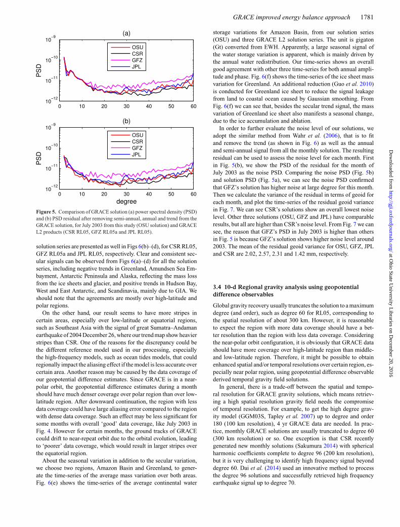
terms of geoid undulation, using all the geopotential differencesfrom Fig. 4(a). For comparison, the geoid maps from other threeL2 solutions for the month of July 2003 are also shown in theright column of Fig. 4 (Fig. 4d for CSR RL05, Fig. 4f for GFZRL05a and Fig. 4h for JPL RL05). Here we did not apply any post-processing techniques except that we replace the C20 coefficientsusing the values obtained from satellite laser ranging (Cheng et al.2013). Although the input geopotential differences in the left-handcolumn of Fig. 4(a) seem to agree with the predicted value, thisdoes not necessarily guarantee the recovered solution should besimilar as well. In fact, the high frequency signal and noise inFig. 4(a) could still leak into the low frequency band during theinversion process. Therefore, after downward continuation fromsatellite altitude to Earth surface, enlarged noise, that is north-to-south stripes, should be expected in the gravity solution, which canbe seen from Fig. 4(b). Compared Fig. 4(b) and other three figures inthe right-hand column of Fig. 4, the geoid undulation map from oursolution (OSU) has fewer stripes than the JPL or the GFZ solution,but slightly more stripes than the CSR solution, for this particularmonth. The comparison of Power Spectral Density (PSD) is shownin Fig. 5(a). We can see at lower degree (below degree 15), ourPSD (OSU) matches other three PSDs very well, which means oursolution contains highly consistent time-variable gravity signal. Athigher degree (above degree 15), our PSD shows similar noise levelas JPL’s PSD, which is slightly higher than CSR’s PSD but lowerthan GFZ’s PSD.

3.3 Secular and seasonal gravity variation from globalsolutions

The primary goal of GRACE mission is to map the temporal vari-ation of Earth’s gravity field, for the purpose to understand themass transports within the Earth system. Using the same method,we generate a series of monthly gravity solutions up to degree andorder 60 from 2003 to 2013. Then we estimate the secular and sea-sonal variation based on our solution series. Fig. 6(a) shows theestimated secular variation from 2003 to 2013, in terms of equiv-alent water height (EWH) change. Unlike the geoid map shown inFig. 3, the EWH map normally contains heavier stripes caused bythe amplification of high-frequency noise. Therefore, we applied a150 km radius Gaussian smoothing (Wahr et al. 1998) to mitigatethe error. For comparison, three EWH trend maps from GRACE L2

at Ohio State U


ecember 20, 2016


ownloaded from



Figure 4. Global map of both geopotential difference estimates and recovered gravity solution for the month of July 2003. Left-hand panel: geopotentialdifferences (a) estimated from this study (OSU) and predicted from GRACE L2 products of (c) CSR RL05, (e) GFZ RL05a and (g) JPL RL05. Right-handpanel: recovered geoid undulation from (b) this study using geopotential difference estimates (OSU) and from GRACE L2 products of (d) CSR RL05, (f) GFZRL05a and (g) JPL RL05.

at Ohio State U


ecember 20, 2016


ownloaded from



Figure 5. Comparison of GRACE solution (a) power spectral density (PSD)and (b) PSD residual after removing semi-annual, annual and trend from theGRACE solution, for July 2003 from this study (OSU solution) and GRACEL2 products (CSR RL05, GFZ RL05a and JPL RL05).

solution series are presented as well in Figs 6(b)–(d), for CSR RL05,GFZ RL05a and JPL RL05, respectively. Clear and consistent sec-ular signals can be observed from Figs 6(a)–(d) for all the solutionseries, including negative trends in Greenland, Amundsen Sea Em-bayment, Antarctic Peninsula and Alaska, reflecting the mass lossfrom the ice sheets and glacier, and positive trends in Hudson Bay,West and East Antarctic, and Scandinavia, mainly due to GIA. Weshould note that the agreements are mostly over high-latitude andpolar regions.

On the other hand, our result seems to have more stripes incertain areas, especially over low-latitude or equatorial regions,such as Southeast Asia with the signal of great Sumatra–Andamanearthquake of 2004 December 26, where our trend map show heavierstripes than CSR. One of the reasons for the discrepancy could bethe different reference model used in our processing, especiallythe high-frequency models, such as ocean tides models, that couldregionally impact the aliasing effect if the model is less accurate overcertain area. Another reason may be caused by the data coverage ofour geopotential difference estimates. Since GRACE is in a near-polar orbit, the geopotential difference estimates during a monthshould have much denser coverage over polar region than over low-latitude region. After downward continuation, the region with lessdata coverage could have large aliasing error compared to the regionwith dense data coverage. Such an effect may be less significant forsome months with overall ‘good’ data coverage, like July 2003 inFig. 4. However for certain months, the ground tracks of GRACEcould drift to near-repeat orbit due to the orbital evolution, leadingto ‘poorer’ data coverage, which would result in larger stripes overthe equatorial region.

About the seasonal variation in addition to the secular variation,we choose two regions, Amazon Basin and Greenland, to gener-ate the time-series of the average mass variation over both areas.Fig. 6(e) shows the time-series of the average continental water

storage variations for Amazon Basin, from our solution series(OSU) and three GRACE L2 solution series. The unit is gigaton(Gt) converted from EWH. Apparently, a large seasonal signal ofthe water storage variation is apparent, which is mainly driven bythe annual water redistribution. Our time-series shows an overallgood agreement with other three time-series for both annual ampli-tude and phase. Fig. 6(f) shows the time-series of the ice sheet massvariation for Greenland. An additional reduction (Guo et al. 2010)is conducted for Greenland ice sheet to reduce the signal leakagefrom land to coastal ocean caused by Gaussian smoothing. FromFig. 6(f) we can see that, besides the secular trend signal, the massvariation of Greenland ice sheet also manifests a seasonal change,due to the ice accumulation and ablation.

In order to further evaluate the noise level of our solutions, weadopt the similar method from Wahr et al. (2006), that is to fitand remove the trend (as shown in Fig. 6) as well as the annualand semi-annual signal from all the monthly solution. The resultingresidual can be used to assess the noise level for each month. Firstin Fig. 5(b), we show the PSD of the residual for the month ofJuly 2003 as the noise PSD. Comparing the noise PSD (Fig. 5b)and solution PSD (Fig. 5a), we can see the noise PSD confirmedthat GFZ’s solution has higher noise at large degree for this month.Then we calculate the variance of the residual in terms of geoid foreach month, and plot the time-series of the residual geoid variancein Fig. 7. We can see CSR’s solutions show an overall lowest noiselevel. Other three solutions (OSU, GFZ and JPL) have comparableresults, but all are higher than CSR’s noise level. From Fig. 7 we cansee, the reason that GFZ’s PSD in July 2003 is higher than othersin Fig. 5 is because GFZ’s solution shows higher noise level around2003. The mean of the residual geoid variance for OSU, GFZ, JPLand CSR are 2.02, 2.57, 2.31 and 1.42 mm, respectively.

3.4 10-d Regional gravity analysis using geopotentialdifference observables

Global gravity recovery usually truncates the solution to a maximumdegree (and order), such as degree 60 for RL05, corresponding tothe spatial resolution of about 300 km. However, it is reasonableto expect the region with more data coverage should have a bet-ter resolution than the region with less data coverage. Consideringthe near-polar orbit configuration, it is obviously that GRACE datashould have more coverage over high-latitude region than middle-and low-latitude region. Therefore, it might be possible to obtainenhanced spatial and/or temporal resolutions over certain region, es-pecially near polar region, using geopotential difference observablederived temporal gravity field solutions.

In general, there is a trade-off between the spatial and tempo-ral resolution for GRACE gravity solutions, which means retriev-ing a high spatial resolution gravity field needs the compromiseof temporal resolution. For example, to get the high degree grav-ity model (GGM03S, Tapley et al. 2007) up to degree and order180 (100 km resolution), 4 yr GRACE data are needed. In prac-tice, monthly GRACE solutions are usually truncated to degree 60(300 km resolution) or so. One exception is that CSR recentlygenerated new monthly solutions (Sakumura 2014) with sphericalharmonic coefficients complete to degree 96 (200 km resolution),but it is very challenging to identify high frequency signal beyonddegree 60. Dai et al. (2014) used an innovative method to processthe degree 96 solutions and successfully retrieved high frequencyearthquake signal up to degree 70.

at Ohio State U


ecember 20, 2016


ownloaded from



Figure 6. Secular and seasonal gravity variation. Top and middle rows: Trend map (in terms of equivalent water height rate in mm yr–1) for period from 2003to 2013 (a) estimated from this study and from GRACE L2 products of (b) CSR RL05, (c) GFZ RL05a and (d) JPL RL05, 150 km Gaussian smoothing applied.Bottom row: Time-series of secular and seasonal mass variation (in Gigaton) for (e) Amazon Basin and (f) Greenland, additional leakage reduction applied.

Figure 7. Residual rms (2003–2013) after removing trend, annual and semi-annual signal from all the monthly solutions, based on the results from thisstudy (OSU) and GRACE L2 products (CSR RL05, GFZ RL05a and JPLRL05).

On the other hand, several attempts have been made to improve thetemporal resolution of GRACE. For example, GFZ routinely gener-ates weekly solutions, but only up to degree and order 30. Bruinsmaet al. (2010) generate the 10-d solutions up to degree and order 50with regularization based on traditional dynamic method. Kurten-bach et al. (2009) employed short-arc method (Mayer-Gurr et al.2007) under the principle of Kalman smoothing to conduct the dailysnapshot solution, but the stochastic behaviour of the gravity fieldhas to be considered as a priori information. Kang et al. (2008) usedtraditional dynamic method to generate the so-called ‘quick-look’solution with a moving-window strategy (with a window step of oneday and window width of 15 d), but those solutions are also stabi-lized using regularization. An incomplete list of GRACE solutionswith various temporal resolutions from different research groups canbe found at http://icgem.gfz-potsdam.de/ICGEM/TimeSeries.html.

at Ohio State U


ecember 20, 2016


ownloaded from

http://icgem.gfz-potsdam.de/ICGEM/TimeSeries.html.



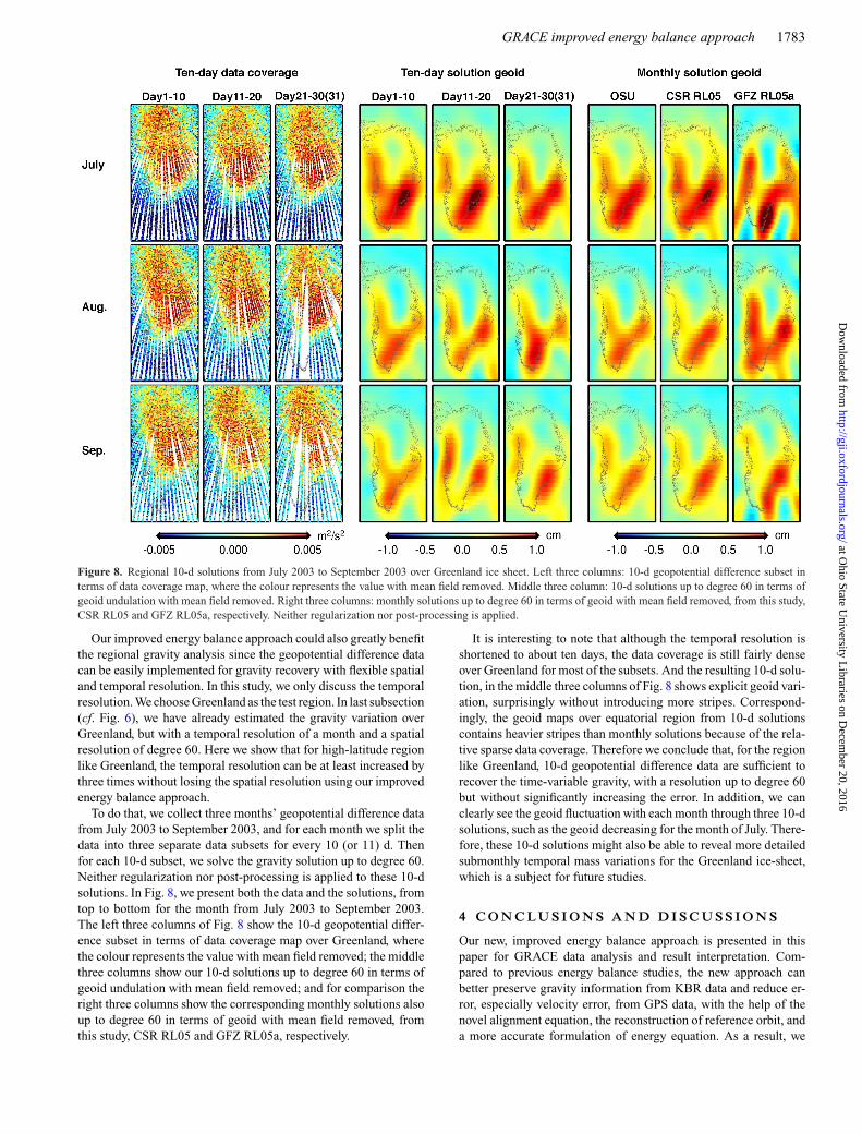
Figure 8. Regional 10-d solutions from July 2003 to September 2003 over Greenland ice sheet. Left three columns: 10-d geopotential difference subset interms of data coverage map, where the colour represents the value with mean field removed. Middle three column: 10-d solutions up to degree 60 in terms ofgeoid undulation with mean field removed. Right three columns: monthly solutions up to degree 60 in terms of geoid with mean field removed, from this study,CSR RL05 and GFZ RL05a, respectively. Neither regularization nor post-processing is applied.

Our improved energy balance approach could also greatly benefitthe regional gravity analysis since the geopotential difference datacan be easily implemented for gravity recovery with flexible spatialand temporal resolution. In this study, we only discuss the temporalresolution. We choose Greenland as the test region. In last subsection(cf. Fig. 6), we have already estimated the gravity variation overGreenland, but with a temporal resolution of a month and a spatialresolution of degree 60. Here we show that for high-latitude regionlike Greenland, the temporal resolution can be at least increased bythree times without losing the spatial resolution using our improvedenergy balance approach.

To do that, we collect three months’ geopotential difference datafrom July 2003 to September 2003, and for each month we split thedata into three separate data subsets for every 10 (or 11) d. Thenfor each 10-d subset, we solve the gravity solution up to degree 60.Neither regularization nor post-processing is applied to these 10-dsolutions. In Fig. 8, we present both the data and the solutions, fromtop to bottom for the month from July 2003 to September 2003.The left three columns of Fig. 8 show the 10-d geopotential differ-ence subset in terms of data coverage map over Greenland, wherethe colour represents the value with mean field removed; the middlethree columns show our 10-d solutions up to degree 60 in terms ofgeoid undulation with mean field removed; and for comparison theright three columns show the corresponding monthly solutions alsoup to degree 60 in terms of geoid with mean field removed, fromthis study, CSR RL05 and GFZ RL05a, respectively.

It is interesting to note that although the temporal resolution isshortened to about ten days, the data coverage is still fairly denseover Greenland for most of the subsets. And the resulting 10-d solu-tion, in the middle three columns of Fig. 8 shows explicit geoid vari-ation, surprisingly without introducing more stripes. Correspond-ingly, the geoid maps over equatorial region from 10-d solutionscontains heavier stripes than monthly solutions because of the rela-tive sparse data coverage. Therefore we conclude that, for the regionlike Greenland, 10-d geopotential difference data are sufficient torecover the time-variable gravity, with a resolution up to degree 60but without significantly increasing the error. In addition, we canclearly see the geoid fluctuation with each month through three 10-dsolutions, such as the geoid decreasing for the month of July. There-fore, these 10-d solutions might also be able to reveal more detailedsubmonthly temporal mass variations for the Greenland ice-sheet,which is a subject for future studies.

4 C O N C LU S I O N S A N D D I S C U S S I O N S

Our new, improved energy balance approach is presented in thispaper for GRACE data analysis and result interpretation. Com-pared to previous energy balance studies, the new approach canbetter preserve gravity information from KBR data and reduce er-ror, especially velocity error, from GPS data, with the help of thenovel alignment equation, the reconstruction of reference orbit, anda more accurate formulation of energy equation. As a result, we

at Ohio State U


ecember 20, 2016


ownloaded from



obtain more accurate geopotential difference estimates with highercorrelation (more than 0.9) with official GRACE RL05 monthlysolutions. Using the resulting geopotential difference estimates, wedemonstrate the global solution is feasible, and for the first time,produce an independent series of GRACE monthly global solu-tions based on energy balance principle, with consistent secularand seasonal time-variable gravity signals compared to other so-lutions based on dynamic method. Furthermore, we show that ourimproved geopotential difference data can be applied for gravityrecovery with flexible temporal resolution, which is conducted overGreenland ice sheets and achieve a higher temporal resolution at10-d interval, as compared to the official monthly solutions, withoutthe compromise of spatial resolution, nor the need to use regular-ization or post-processing. It is worth mentioning that our purposeis to only demonstrate that our method mimics the accuracy of L2products. We are not implying that our global solution based on en-ergy approach is better, that is more accurate and/or higher spatialresolution, than other products.

Our new method would also benefit data analysis of the forth-coming GRACE follow-on mission, especially considering the pos-sibility that the precision of range-rate data can be improved by upto a factor of 20 (Loomis et al. 2012), but the precision of GPStracking data may not have significant advances. In that case, theweighting of GPS tracking data would need to be further reducedfor the traditional conventional dynamic method, which could bemore analogous to our method since we have already handle GPSdata and range-rate data separately through the alignment equation.Therefore, our energy balance method might have a unique contri-bution to the processing of more accurate data from next generationsatellite gravimetry mission to study mass transports of the Earth.

A C K N OW L E D G E M E N T S

This research is supported by grants from NSF via the BelmontForum/IGFA (ICER-1342644), NASA’s geodesy and cryosphere(NNX12AK28G, NNX13AQ89G, and NNX11AR47G), State KeyLaboratory of Geodesy and Earth’s Dynamics, Institute of Geodesy& Geophysics, Chinese Academy of Sciences (Y309473047,SKLGED2015-5-3-E), and Natural Science Foundation of China(NSFC, 41374020). GRACE data products are from NASA’s PO-DAAC via JPL, CSR and GFZ. Some figures in this paper weregenerated using the Generic Mapping Tools (GMT; Wessel & Smith1991). The computational aspect of this work was supported in partby an allocation of computing resources from the Ohio Supercom-puter Center (http://www.osc.edu). We thank Tzupang Tseng, Na-tional Central University, Taiwan, Adrian Jaggi, University of Bernand Dahning Yuan, Jet Propulsion Laboratory, California Instituteof Technology for providing precise GRACE orbits. We acknowl-edge the German Space Operations Center (GSOC) of the GermanAerospace Center (DLR) for providing continuously and nearly 100per cent of the raw telemetry data of the twin GRACE satellites. Wethank two anonymous reviewers and the editor for their helpful andconstructive comments leading to improvement of the manuscript.

R E F E R E N C E S

Badura, T., Sakulin, C., Gruber, C. & Klostius, R., 2006. Derivation of theCHAMP-only global gravity field model TUG-CHAMP04 applying theenergy integral approach, Stud. Geophys. Geod., 50(1), 59–74.

Biancale, R. & Bode, A., 2006. Mean annual and seasonal atmospherictide models based on 3-hourly and 6-hourly ECMWF surface pressure

data, Tech. Rep., Potsdam, Deutsches GeoForschungsZentrum GFZ, doi:http://doi.org/10.2312/GFZ.b103–06011.

Bjerhammar, A., 1969. On the energy integral for satellites, Tellus, 21,1–9.

Bruinsma, S., Lemoine, J. M., Biancale, R. & Vales, N., 2010. CNES/GRGS10-day gravity field models (release 2) and their evaluation, Adv. SpaceRes., 45(4), 587–601.

Cazenave, A. & Chen, J., 2010. Time-variable gravity from space andpresent-day mass redistribution in the Earth system, Earth planet. Sci.Lett., 298(3), 263–274.

Chen, Y.Q., Schaffrin, B. & Shum, C.K., 2008. Continental water stor-age changes from GRACE Line-of-sight range acceleration measure-ments, in VI Hotine-Marussi Symposium on Theoretical and Com-putational Geodesy , Vol. 132, ISSN, pp. 62–66, eds Peiliang, Xu,Jingnan, Liu & Athanasios, Dermanis, International Association ofGeodesy Symposia, doi:10.1007978–3–540–74584–6.

Cheng, M., Tapley, B.D. & Ries, J.C., 2013. Deceleration in the Earth’soblateness, J. geophys. Res.: Solid Earth, 118, 740–747.

Dai, C., Shum, C.K., Wang, R., Guo, J., Shang, K., Tapley, B. & Wang,L., 2014. Improved source parameter constraints for recent large under-sea earthquakes from high-degree GRACE gravity and gravity gradientchange measurements, in Proceedings of the AGU Fall Meeting, SanFrancisco, CA, USA, 15–19 December 2014.

Dahle, C., Flechtner, F., Gruber, C., Konig, D., Konig, R., Michalak, G. &Neumayer, K.-H., 2012. GFZ GRACE level-2 processing standards doc-ument for level-2 product release 0005, Tech. Rep., Potsdam, DeutschesGeoForschungsZentrum GFZ, doi:10.2312/GFZ.b103–12020.

Ditmar, P. & van Eck van der Sluijs, A.A., 2004. A technique for Earth’sgravity field modeling on the basis of satellite accelerations, J. Geod., 78,12–33.

Ditmar, P, Teixeira da Encarnacao, J. & Hashemi Farahani, H., 2012. Un-derstanding data noise in gravity field recovery on the basis of inter-satellite ranging measurements acquired by the satellite gravimetry mis-sion GRACE, J. Geod., 86, 441–465.

Gerlach, C. et al., 2003. A CHAMP-only gravity field model from kine-matic orbits using the energy integral, Geophys. Res. Lett., 30(20), 2037,doi:10.1029/2003GL018025.

Guo, J.Y., Duan, X.J. & Shum, C.K., 2010. Non-isotropic Gaussian smooth-ing and leakage reduction for determining mass changes over land andocean using GRACE data, Geophys. J. Int., 181, 290–302.

Guo, J.Y., Shang, K., Jekeli, C. & Shum, C.K., 2015. On the energy inte-gral formulation of gravitational potential differences from satellite-to-satellite tracking, Celest. Mech. Dyn. Astr, 121(4), 415–429.

Han, S.-C., 2003. Efficient global gravity determination from satellite-to-satellite tracking (SST), Diss. PhD thesis, Geodetic and GeoinformationScience, Department of Civil and Environmental Engineering and Geode-tic Science, The Ohio State University, Columbus, OH, USA.

Han, S.-C., Jekeli, C. & Shum, C.K., 2002. Efficient gravity field recoveryusing in situ disturbing potential observables from CHAMP, Geophys.Res. Lett., 29(16), 1789, doi:10.1029/2002GL015180.

Han, S.-C., Shum, C.K., Jekeli, C. & Alsdorf, D., 2005. Improved estimationof terrestrial water storage changes from GRACE, Geophys. Res. Lett.,32, L07302, doi:10.1029/2005GL022382.

Han, S.-C., Shum, C.K. & Jekeli, C., 2006. Precise estimation of in situgeopotential differences from GRACE low-low satellite-to-satellite track-ing and accelerometer data, J. geophys. Res., 111, B04411, doi:10.1029/2005JB003719.

Jaggi, A., Bock, H., Pail, R. & Goiginger, H., 2008. Highly-reduced dynamicorbits and their use for global gravity field recovery: a simulation studyfor GOCE, Stud. Geophys. Geod., 52(3), 341–359.

Jekeli, C., 1999. The determination of gravitational potential differencesfrom satellite-to-satellite tracking, Celestial Mech. Dyn. Astron., 75, 85–100.

Jekeli, C., 2001. Inertial Navigation Systems with Geodetic Applications,Walter de Gruyter.

Kang, Z., Tapley, B., Bettadpur, S., Ries, J., Nagel, P. & Pastor, R., 2006.Precise orbit determination for the GRACE mission using only GPS data,J. Geod., 80(6), 322–331.

at Ohio State U


ecember 20, 2016


ownloaded from

http://www.osc.edu



Kang, Z., Bettadpur, S., Nagel, P., Pastor, R., Pekker, T., Poole, S. &Tapley, B., 2008. Quick-look gravity solutions from GRACE, in Proceed-ings of the AGU Fall Meeting 2008, San Francisco, CA, 15–19 December,2008.

Kurtenbach, E., Mayer-Gurr, T. & Eicker, A., 2009. Deriving daily snapshotsof the Earth’s gravity field from GRACE L1B data using Kalman filtering,Geophys. Res. Lett., 36, L17102, doi:10.1029/2009GL039564.

Liu, X., Ditmar, P., Siemes, C., Slobbe, D.C., Revtova, E., Klees, R., Riva,R. & Zhao, Q., 2010. DEOS Mass Transport model (DMT-1) based onGRACE satellite data: methodology and validation. Geophys. J. Int., 181,769–788.

Loomis, B.D., Nerem, R.S. & Luthcke, S.B., 2012. Simulation study of afollow-on gravity mission to GRACE. J. Geod., 86(5), 319–335.

Luthcke, S.B., Rowlands, D.D., Lemoine, F.G., Klosko, S.M., Chinn, D. &McCarthy, J.J., 2006. Monthly spherical harmonic gravity field solutionsdetermined from GRACE inter-satellite range-rate data alone, Geophys.Res. Lett., 33, L02402, doi:10.1029/2005GL024846.

Mayer-Gurr, T., Eicker, A. & Ilk, K.H., 2007. ITG-Grace02s: a GRACEgravity field derived from range measurements of short arcs, in GravityField of the Earth: Proceedings of the 1st International Symposium of theInternational Gravity Field Service (IGFS), Special Issue 18, pp. 193–198, eds Kilicoglu, A. & Forsberg, R., Gen. Command of Mapp., Ankara,Turkey.

Mayer-Gurr, T., Savcenko, R., Bosch, W., Daras, I., Flechtner, F. & Dahle,C., 2012. Ocean tides from satellite altimetry and GRACE, J. Geod.,59–60, 28–38.

Meyer, U., Jaggi, A. & Beutler, G., 2012. Monthly gravity field solutionsbased on GRACE observations generated with the Celestial MechanicsApproach, Earth planet. Sci. Lett., 345, 72–80.

Pail, R. et al., 2011. First GOCE gravity field models derived by threedifferent approaches, J. Geod., 85(11), 819–843.

Petit, G. & Luzum, B., 2010. IERS Conventions (2010). IERS TechnicalNote No. 36. Verlag des Bundesamts fur Kartographie und Geodasie,Frankfurt am Main.

Ramillien, G., Biancale, R., Gratton, S., Vasseur, X. & Bourgogne, S.,2011. GRACE-derived surface water mass anomalies by energy in-tegral approach: application to continental hydrology, J. Geod., 6,313–328.

Ries, J.C., Bettadpur, S., Poole, S. & Richter, T., 2011. Mean backgroundgravity fields for GRACE processing, in Proceedings of the GRACE Sci-ence Team Meeting, Austin, TX, 8–10 August 2011.

Rowlands, D.D., Ray, R.D., Chinn, D.S. & Lemoine, F.G., 2002. Short-arcanalysis of intersatellite tracking data in a gravity mapping mission, J.Geod., 76, 307–316.

Rowlands, D.D., Luthcke, S.B., Klosko, S.M., Lemoine, F.G.R., Chinn, D.S.,McCarthy, J.J., Cox, C.M. & Anderson, O.B., 2005. Resolving mass flux athigh spatial and temporal resolution using GRACE intersatellite measure-ments, Geophys. Res. Lett., 32, L04310, doi:10.1029/2004GL021908.

Rowlands, D.D., Luthcke, S.B., McCarthy, J.J., Klosko, S.M., Chinn, D.S.,Lemoine, F.G., Boy, J.-P. & Sabaka, T.J., 2010. Global mass flux solutionsfrom GRACE: a comparison of parameter estimation strategies—massconcentrations versus Stokes coefficients, J. geophys. Res., 115, B01403,doi:10.1029/2009JB006546.

Sakumura, C., 2014. Comparison of Degree 60 and Degree 96 MonthlySolutions, GRACE Technical Note 10. http://www.csr.utexas.edu/grace/TN10_CSR-GR-14–01.pdf, last accessed September2015

Schmidt, M., Han, S.-C., Kusche, J., Sanchez, L. & Shum, C.K.,2006. Regional high-resolution spatiotemporal gravity modeling fromGRACE data using spherical wavelets, Geophys. Res. Lett., 33, L08403,doi:10.1029/2005GL025509.

Schmidt, M., Seitz, F. & Shum, C.K., 2008. Regional four-dimensionalhydrological mass variations from GRACE, atmospheric flux con-vergence, and river gauge data, J. geophys. Res., 113, B10402,doi:10.1029/2008JB005575.

Tangdamrongsub, N., Hwang, C., Shum, C.K. & Wang, L., 2012. Regionalsurface mass anomalies from GRACE KBR measurements: application ofL-curve regularization and a priori hydrological knowledge, J. geophys.Res., 117, B11406, doi:10.1029/2012JB009310.

Tapley, B.D., Bettadpur, S., Watkins, M. & Reigber, C., 2004a. The gravityrecovery and climate experiment: mission overview and early results,Geophys. Res. Lett., 31, L09607, doi:10.1029/2004GL019920.

Tapley, B.D., Schutz, B. & Born, G.H., 2004b. Statistical Orbit Determina-tion, Elsevier.

Tapley, B.D., Ries, J., Bettadpur, S., Chambers, D., Cheng, M., Condi, F. &Poole, S., 2007. The GGM03 mean earth gravity Model from GRACE,in Proceedings of the AGU Fall Meeting 2007, San Francisco, CA, 10–14December, 2007.

Visser, P.N.A.M., Sneeuw, N. & Gerlach, C., 2003. Energy integral methodfor gravity field determination from satellite orbit coordinates, J. Geod.,77, 207–216.

Wahr, J., Molenaar, M. & Bryan, F., 1998. Time variability of theEarth’s gravity field: hydrological and oceanic effects and their pos-sible detection using GRACE, J. geophys. Res., 103(B12), 30 205–30 229.

Wahr, J., Swenson, S. & Velicogna, I., 2006. Accuracy of GRACE massestimates, Geophys. Res. Lett., 33, L06401, doi:10.1029/2005GL025305.

Wang, X., Gerlach, C. & Rummel, R., 2012. Time-variable gravity fieldfrom satellite constellations using the energy integral, Geophys. J. Int.,190(3), 1507–1525.

Wessel, P. & Smith, W.H.F., 1991. Free software helps map and display data,EOS, Trans. Am. geophys. Un., 72(41), 441, doi:10.1029/90EO00319.

Yi, W., 2012. The Earth’s gravity field from GOCE, PhD dissertation,Munchen, Technische Universitat Munchen.

A P P E N D I X : E N E RG Y E Q UAT I O N S I NI N E RT I A L A N D E A RT H - F I X E D F R A M E

A1. Preliminary

The position vector r, representing the satellite position relativeto Earth centre, can be expanded in any Cartesian coordinateframe s (called s-frame) as an ordered triplet of coordinates as

rs = (r s

1 r s2 r s

3

)T, such as inertial frame (i-frame) as ri, and Earth-

fixed frame (e-frame) as re. The relation between the two coordinatevectors can be described as

ri = Ciere, (A1)

where Cie is a transformation matrix representing the orientation

between the two frames. The time-derivative of Cie can be derived

using the angular velocity w between the two frames. Here we definewi

ie = (ω1, ω2, ω3)T as the angular velocity vector of the e-framewith respect to the i-frame, with coordinates in the i-frame. Thecross-product of the angular velocity vector can be further writtenas a skew-symmetric matrix

[wi

ie×] = i

ie =

⎛⎜⎜⎝

0 −ω3 ω2

ω3 0 −ω1

−ω2 ω1 0

⎞⎟⎟⎠ .

Using above notations, we can derive the time-derivative of thetransformation matrix Ci

e as (Jekeli 2001)

C ie = −i

ei Cie = i

ieCie = Ci

eeie = [

wiie×

]Ci

e = Cie

[we

ie×].

Therefore, taking the time-derivative of (A1) yields

ri = Cie re + C i

ere = Cie

(re + we

ie × re), (A2)

at Ohio State U


ecember 20, 2016


ownloaded from

http://www.csr.utexas.edu/grace/TN10_CSR-GR-14--01.pdf

http://www.csr.utexas.edu/grace/TN10_CSR-GR-14--01.pdf



which represent the transformation of the velocity vector betweentwo frames. Taking another time-derivative of (A2) yields

ri = Cie re + 2Ci

e

(we

ie × re) + Ci

e

[we

ie × (we

ie × re)]

, (A3)

which represents the transformation of the acceleration vector be-tween two frames. Here we need to assume wie = wi

ie = weie = 0,

which is the first assumption for energy equations.

A2. Newton’s law of motion in both frames

Acceleration vector in i-frame must obey Newton’s law of motion,which says

ri = ∇ i V E + ai , (A4)

where ∇ i = (∂

∂r i1

∂

∂r i2

∂

∂r i3

)T represents the gradient operator in i-

frame, VE is Earth’s static as well as secular and seasonal time-variable geopotential, and ai = ∇ i V R + f i represent the sum of theacceleration from residual geopotential VR and non-conservativeforce f.

In e-frame, Newton’s law of motion can be derived using eqs(A3) and (A4) as

re = ∇eV E + ae − 2(we

ie × re) − [

weie × (

weie × re

)], (A5)

where all quantities are represented in e-frame.

A3. Time-derivative of static geopotential in both frames

In i-frame, the time-derivative of VE can be expanded as

V E = dV E

dt= ∂V E

∂t

∣∣∣∣i

+ (∇ i V E )T · ri . (A6)

The same is for e-frame where the time-derivative of VE can beexpanded as

V E = dV E

dt= ∂V E

∂t

∣∣∣∣e

+ (∇eV E )T · re. (A7)

Here we introduce the second assumption that (∂V E/∂t)

∣∣e = 0since we need to assume that for a certain time interval VE has to bestatic, that is the partial derivative with respect to time in e-frameshould be zero.

Next we need to rewrite eqs (A6) and (A7) by eliminating VE

from the right-hand side. Combining (A6) and (A7) by consideringthe second assumption, we have

∂V E

∂t

∣∣∣∣i

= (∇ i V E)T (

Cie re − ri

).

Substituting the above equation into (A6) by considering (A2)and Newton’s law in i-frame (A4), we can rewrite eq. (A6), thetime-derivative of static geopotential in i-frame, as

dV E

dt= (

ri − ai) · (

ri − wiie × ri

). (A8)

In e-frame, multiplying re to (A5), we have

re · re = ∇eV E · re + ae · re − 2(we

ie × re) · re

− [we

ie × (we

ie × re)] · re,

where the third term on the right-hand side is zero. Substituting theabove equation into (A7) by considering the second assumption, wecan rewrite eq. (A7), the time-derivative of static geopotential ine-frame, as

dV E

dt= [

re − ae + weie × (

weie × re

)] · re. (A9)

Clearly (A8) and (A9) are equivalent since they are both derivedfrom the same equations and the same two assumptions; that is, wecan easily show

dV E

dt= (

ri − ai) · (

ri − wiie × ri

)= [

re − ae + weie × (

weie × re

)] · re

= (∇eV E)T · re.

A4. Energy equation in both frames

The energy equation in i-frame is obtained by integrating (A8) withrespect to time as

V E =∫ t

t0

(ri − ai

) · (ri − wi

ie × ri)

dt .

Since wiie = 0, we arrive at the formulation of energy equation

in i-frame as follows:

V E = 1

2

∣∣ri∣∣2 − wi

ie · (ri × ri

) −∫ t

t0

ai · (ri − wi

ie × ri)

dt − E0i .

(A10)

Similarly, the energy equation in e-frame is obtained by integrating(9) with respect to time as

V E =∫ t

t0

[re − ae + we

ie × (we

ie × re)] · redt .

Since weie = 0 as well, we arrive at the formulation of energy

equation in e-frame as follows:

V E = 1

2|re|2 − 1

2

∣∣weie × re

∣∣2 −∫ t

t0

ae · redt − E0e. (A11)

Again, (A10) and (A11) are equivalent just as (A8) and (A9).Finally, it should be noticed that in both frames

∫ tt0

a · rdt �=V R + ∫ t

t0f · rdt , since residual geopotential VR (such as tides) is not

static in either frames. We mention that some previous studies havealready derived the identical (e.g. Gerlach et al. 2003; Han 2003;Wang et al. 2012) or similar (e.g. Badura et al. 2006; Jaggi et al.2008) formulation.

at Ohio State U


ecember 20, 2016


ownloaded from


geophysical journal international - geodesy.geology.ohio

Documents