geophysics and wine in new zealand -...

1

Geophysics and Wine in New Zealand

Stephen P. Imre1,2 and Jeffrey L. Mauk1 1University of Auckland

2Worley Parsons Canada 1New Zealand,

2Canada

1. Introduction

The New Zealand wine industry is committed to producing high quality, market led wines (New Zealand Winegrowers, 2009). Consequently for the industry, it is imperative to understand what factors influence grape and wine properties in order to maximise the production of premium wines. New Zealand winegrowing regions produce different styles of wine, yet there is little data to build an understanding of what contributes to the quality of New Zealand wines both on regional and local scales. On a global scale, the New Zealand industry accounts for less than 0.03% of land under vine and less than 0.5% of global wine production (New Zealand Winegrowers, 2009), and yet it adds an estimated $4 billion to the New Zealand economy (NZIER, 2009). Global area under vine in 2006 was roughly 7,812,000 ha, and wine production was approximately 282,000,000 hl (Organisation Internationale de la Vigne et du Vin [OIV], 2006). Quantifying variables that may influence grape/wine parameters may aid in creating a better understanding of what factors influence wine characteristics. This research demonstrates that vine growth is variable in uniformly managed blocks, and geophysical tools can be used to map soil variability in vineyards, which in turn can influence grapevine vigour and presumably grape properties. Terroir can be defined as the physical and chemical characteristics of a vineyard or region,

including geology, soils, topography, and climate. Different terroirs have been delineated in

Europe based largely on areas that have produced distinctive wines over a long period of

time (White, 2003). These areas are typically delineated using geographical indicators such

as geology, soil, topography and mesoclimate. The influence of winemaker and cultural

practices can also be considered part of terroir. These environmental properties and cultural

practices interact to create wine with particular characteristics, and the place of origin

ultimately influences the wines produced. Terroir forms the basis for appellation d’origine

controlée (AOC), the vineyard classification system used in France in areas such as

Bordeaux, Burgundy, and Champagne, with wine produced from particular terroirs being

associated with a certain quality and wine style (Wilson, 1998).

Several publications have emerged on different facets of terroir at various scales, indicating an increased interest in the subject. For example, Swinchatt & Howell (2004) explore the terroir of the Napa Valley examining its geology, history and environment. Haeger (2004) discusses the rise of Pinot Noir in North America and its associated terroirs. Wilson (1998) discusses the terroir of selected areas in France. Geoscience Canada has a series devoted to

www.intechopen.com

Earth and Environmental Sciences

4

geology and wine from various winegrowing regions of the world (Macqueen & Meinert, 2006). Terroir studies have also been conducted on a vineyard-block scale examining local variations in properties such as microclimate and soils (e.g. Trought et al., 2008). A summary of national-regional terroir in New Zealand is described in Imre & Mauk (2009). Grapevine trunk circumference measurements can be used as a proxy for variations in

grapevine vigour on a site-specific level (e.g. Clingeleffer & Emmanuelli, 2006; Acevedo-

Opazo et al., 2008; Trought et al., 2008). These localised variations in even small vineyard

blocks can in turn show differences in grape quality parameters (e.g. Cortell et al., 2005;

Trought et al., 2008). If blocks are uniformly managed, changes in soil properties or local

topography may contribute to variations in vine trunk circumference. A rapid cost-effective

method to identify areas of homogeneity in the subsurface, when coupled with GPS

surveys, may provide useful input into site specific variations.

Ground penetrating radar (GPR) and electromagnetic induction (EMI) surveys are

commonly used to map areas of different soil properties (e.g. Kitchen et al., 1996; Doolittle et

al., 2002; James et al., 2003; Hedley et al., 2004; Carroll & Oliver, 2005; Cockx et al., 2007;

Bramley, 2009). The GPR surveys can be useful in measuring depth to soil textural changes

(Simeoni et al., 2009). The EMI surveys are typically single-frequency and measure soil

apparent electrical conductivity (ECa) values at one or two depths (e.g. Bramley, 2001;

Trought et al., 2008), and this can provide very useful data, particularly where crops have a

shallow rooting depth or shallow changes in soil properties are of interest.

Grapevines have rooting depths that may exceed 6 m (Smart et al., 2006 and references therein), and therefore measuring soil ECa values at different depths may be beneficial. Electromagnetic induction surveys have been used to map soil types (e.g. James et al., 2003), and multi-frequency EMI surveys can detect vertical differences in ECa from landfill leachate or buried artefacts where differences among ECa values are large (e.g. Won et al., 1996). If soil ECa changes sufficiently with depth, multi-frequency EMI surveys may be able to provide valuable information about changes in soil with depth. This research demonstrates that geophysical tools can help map variability in soils in vineyards. Soil variability in turn influences grapevine vigour, and presumably the properties of the grapes that are harvested from different areas. Geophysical mapping can help to quantitatively evaluate differences in soils that contribute to variability in the wines that are produced from different areas.

2. Materials and methods

Three vineyard blocks with own-root pinot noir 10/5 on different soil types in Bannockburn, Central Otago were selected for detailed study (Fig. 1). The sites are characterized by a dry climate with mild temperatures and moderate solar radiation (Leathwick et al., 2002; Imre & Mauk, 2009). High vapour pressure deficits and very high annual water deficits make many plantings in the area require irrigation. The study block at Olssens in the north is located on shallow fine sandy loam from shallow loess over fine sand and gravel schist fan alluvium. The Felton Road study block is located on Waenga very deep fine sandy loam from deep alluvium derived from loess, schist and lake bed sediments. Mt Difficulty’s Target Gully site is located on very shallow to shallow fine sandy loam and some deep coarse Otago Schist (Beecroft, 1988; Turnbull, 2000; Leathwick et al., 2002; Imre & Mauk, 2009).

www.intechopen.com


5

Fig. 1. Map of Bannockburn, Central Otago, showing the location of study blocks and associated transects in red, Profile A-A’ in blue. Background colour is soil type as scanned and digitized from Beecroft (1988).

www.intechopen.com


6

2.1 Grapevine physiology Vine trunk circumferences in a selection of rows in each study site were measured at roughly 20 cm above ground level at narrow areas of the vine, and average vine trunk circumference growth in each bay was calculated. Vine trunk circumference measurements can be used as a proxy for vigour variation (e.g. Acevedo-Opazo et al., 2008; Trought et al., 2008). The vines are all on own-root making it unnecessary to take two measurements and average the values because there is no graft union. To remove the influence of abnormally small vines, such as replantings or physically damaged vines (e.g. tractor impact), bays where the smallest vine trunk circumference was less than 70% of the bay average were omitted. The average bay trunk circumferences were then divided into five size classes (extra-small, small, medium, large and extra-large) for each study site, with approximately the same number of values in each class. All vine trunk circumference values refer to average values in each bay.

2.2 Geophysical surveys The SIR 2000 Ground Penetrating Radar unit from Geophysical Survey Systems, Inc (GSSI;

New Hampshire, USA) was used to run transects along each row in the study blocks using a

200 MHz antenna. An electromagnetic wave is emitted from a transmitting antenna, and

part of the wave energy is reflected from changes in soil properties. This radar reflectance is

measured by the receiving antenna and recorded. The GPR data were processed using GSSI

RADAN (RAdar Data ANalyzer) version 6.5, and 3D images of the subsurface down to a

depth of several meters were created. Images were then imported into a GIS (MapInfo

Professional 6.5; Pitney Bowes, New York, USA) and geo-referenced using known GPS

points in the study areas. This allowed for spatial comparison of survey results and vine trunk

circumference data. GPR data showing vertical change are displayed using nanosecond (ns)

instead of depth due mainly to the sharp change in soils and the inability of RADAN

processing software to account for different dielectric properties at depth. A greyscale version

of linescan mode is used to display the data because of its ability to detect gravels within a

sedimentary layer. These gravels, and other isolated objects, cause a diffraction of the

electromagnetic waves resulting in a ringing within the radar signal that is displayed as a

downward parabola (Jol, 2009); this is discussed for each of the figures where appropriate.

One representative transect for each study site is discussed further in this chapter.

For the EMI surveys, a GEM-2 (Geophex, North Carolina, USA) portable handheld broadband electromagnetic sensor connected to a handheld GPS unit was used. Each study block was surveyed using ten frequencies: 1,175 Hz, 2,525 Hz, 3,925 Hz, 7,375 Hz, 10,575 Hz, 13,575 Hz, 25,975 Hz, 35,925 Hz, 44,025 Hz and 47,025 Hz. Higher frequencies measure soil resistivity close to the surface, whereas lower frequencies penetrate to greater depths depending on soil and geology. Soil apparent electrical conductivity (ECa) is then calculated automatically by the GEM-2; the measured resistivity is the inverse of electrical conductivity. 1m x 1m grids were generated from the raw EMI data using triangulation with natural neighbour interpolation in Discover version 4.000 in MapInfo Professional 6.5. These grids allow for mapping of ECa at various depths, and to test whether soil ECa correlates with vine trunk circumference. Maps were then produced at each site from all ten frequencies corresponding to different depths. Generally patterns are clearer at the higher frequencies that represent readings close to the surface. Soil ECa at the frequencies showing the best visual results at each site are presented. Using various combinations of these

www.intechopen.com


7

frequencies as specified for each site individually (Table 1), the data were inverted based on a 1D layered earth model to create depth profiles of apparent soil ECa (Huang & Won, 2003; Huang, 2005). Frequency combinations that gave minimal fit errors when running the inversion algorithm were used. Fit errors are calculated based how the data points fit a semi-variogram of the dataset. A large difference between values will result in a larger fit error. Images were generated to 10 m depth using the inverse distance weighting method in MapInfo 6.5 Professional (Pitney Bowes, New York, USA). All results of the EMI surveys are displayed using histogram equalization stretch for colour display.

Site Frequencies used (Hz)

Profile A-A' 2525, 3925, 7375, 10575, 13575, 25975, 35925, 44025, 47025

Felton Road Wines 1175, 3925, 7375, 25975, 35925

Target Gully 3925, 7375, 13575, 25975, 44025

Olssens 10575, 25975, 35925, 44025, 47025

Table 1. EMI frequencies used at each site for the inversion algorithm

Differential GPS surveys were conducted in all of the study blocks using a Trimble Pro XRS unit (Sunnyvale, California, USA). GPS point data was imported into MapInfo 6.5 Professional and 1m x 1m grids of elevation were created at each site. Slope and aspect were calculated using the Discover 4.000 extension. New Zealand map grid was used for all surveys in the study blocks, and all figures in this chapter are drawn with NZ map grid coordinates.

2.3 Soil sampling and analysis We collected soil profile data from 53 trenches in the study area, and we include selected chemical data from one representative soil profile from each study site in this chapter. Samples were classified into percent gravel, sand, silt and clay using manual sieving for the >2 mm portion and using a Malvern Mastersizer (Malvern Instruments ltd., Worcestershire, UK) for the <2 mm portion. The <2 mm size fraction was analyzed for pH, P, K, Mg, Ca, CEC, Zn, Cu, Al, S, Na, Mn and Fe (Agricultural Analytical Services laboratory, Penn State University, PA, USA; USEPA, 1986; Eckert & Sims, 1995; Ross, 1995; Wolf & Beegle, 1995); the Mehlich 3 extract was used for elemental analysis. Samples were also analyzed for total N and total C at the University of Auckland using the TruSpec CN (LECO Australia Pty Ltd., Castle Hill, NSW, Australia).

2.4 Statistical analyses Statistical analyses were conducted using SPSS 17.0 (SPSS Inc., Chicago, USA) to examine what factors significantly influence vine growth variation. A correlation matrix between all ECa values was initially created to reduce the amount of data by eliminating ECa values at different frequencies that are highly correlated at each site (adjusted-R2>0.9). Stepwise linear regression was then used with vine trunk circumference as the dependent variable and ECa, slope, elevation and aspect data as the predictor variables for each site individually as well as on the total dataset. Eight clusters of slope, elevation and aspect were used as predictor variables in a linear regression analysis both with and without the addition of ECa data. For the stepwise linear regression, the stepping method was set to use probability of F entry=0.05, exit=1.0. Due to the nature of the GPR data, it is not possible to

www.intechopen.com


8

extract values such as those for ECa, and therefore these results were not included in the statistical analysis. Profile A-A’ compares the EMI inversion data with the detailed soil map of Bannockburn in Central Otago (Beecroft, 1988) (Fig. 1, Fig. 9). Multinomial logistic regression analysis was done using SPSS 17.0 (SPSS Inc., Chicago, USA) in order to determine whether significant relationships exist between ECa and mapped soil type (Beecroft, 1988). Mapped soil type is the dependent variable in the analyses, and ECa values at different depths are the covariates as discussed individually for each result. The ECa survey points that are located on roads between vineyard blocks were removed from the analysis.

3. Results

3.1 Vine trunk circumference Vine trunk circumferences vary throughout all study sites (Fig. 2), even though each block is

uniformly managed. Vine trunk circumferences are largest at Felton Road with a median

value of 157 mm, followed by Olssens with a median value of 138 mm, and Target Gully

with the smallest median value of 126 mm. The vines at Felton Road are the largest in the

study, whereas vines are smallest at Target Gully, even though the oldest vines are at

Olssens. The spatial distribution of vine sizes at each site are shown in images later in this

chapter.

Fig. 2. Boxplots showing vine trunk circumference distribution at each block

www.intechopen.com


9

3.2 Felton road wines Vines with small to extra-small trunk circumferences mainly occur in the central eastern area of the block, with some in the south and northwest (Fig. 3a). Vines with medium to large trunk circumferences form a “C”-shaped pattern that surrounds all areas of the block except the central-east, south, and northwest corner. The GPR image shows distinct areas of high amplitude signals in the central-east, south and northeast areas of the study block, and low amplitude signals in a “C” shaped pattern surrounding the higher amplitude areas (Fig. 3a). Two distinct areas of high soil ECa are located in the central-east and southern areas (Fig. 3b). Smaller vines tend to occur in areas with high amplitude GPR signals and higher soil ECa values, suggesting that these soils are less favourable for vine growth. These extremely high soil ECa values generally follow the boundary of a silty loam soil type as verified by extensive soil trenching and as discussed in more detail along Profile A-A’.

Fig. 3. Felton Road Wines showing vine trunk circumference data and a) GPR survey results, and b) EMI survey results

Soil ECa values are very high at the surface and generally decrease with depth (Fig. 4a). An

area of high ECa values occurs in the middle of the row at depths greater than 2 m when

compared to the rest of the row at similar depths. Soil ECa values decrease rapidly at

roughly 2 m depth at the north end, decrease at a more gradual rate throughout the rest of

the row, and remain relatively large in the middle of the row.

www.intechopen.com


10

Fig. 4. Felton Road (a) inversion of EMI survey to 10m depth, (b) GPR transect

The clearest GPR signals are in the north and south ends of the row (Fig. 4b). This area is dominated by hyperbolas, whereby the size and frequency in this geophysical signature indicates the presence of gravels (Jol, 2009). The middle of the row, which contains very high ECa values, has a relatively unclear GPR record that shows alternating layers of blurry and high-amplitude signals.

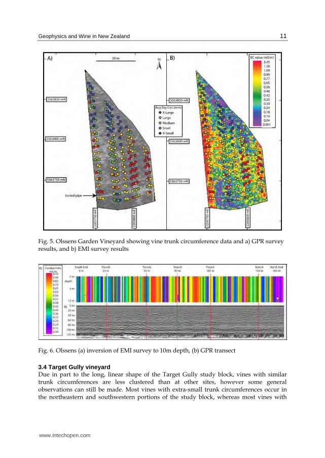
3.3 Olssens garden vineyard Extra-large vine trunk circumferences mainly occur in the central-eastern area, and extra-

small vine trunk circumferences are mainly in the northern portion of the study block (Fig.

5a). The GPR image shows low amplitude signals in the west and high amplitude signals in

the north, east and south (Fig. 5a). The GPR data also distinctly show a buried pipe that runs

from east to west in the southern area of the study block. Two areas of high soil ECa in the

west side and east side of the block coincide with areas that contain vines with large trunk

circumferences (Fig. 5b). Soil ECa values at the site are all below 3.5 mS/m, which is very

low compared to other sites in this study. Soil ECa values are lowest at the Olssens study site, and are typically less than 1 mS/m. The top layer, as defined by the EMI surveys, has an average thickness of greater than 40 m, and therefore the ECa values in our 10 m deep profile do not change with depth (Fig. 6a). The great depth penetration may be due to the little variation in observed soil ECa throughout the profile; over 90% of values are less than 1 mS/m. The centre of the row generally has larger ECa values than the row ends. The upper-most radar signature displays a uniform low-amplitude band down to roughly 20 ns, representing a homogeneous top layer (Fig. 6b). Below this depth reflections are fairly flat-lying with some variation in amplitude, dip, and direction similar to bedding plane deposits imaged using GPR in fluvial settings (Jol, 2009). There is a dipping high-amplitude reflection surface in the southern 50 meters of the image at 110 ns that may indicate a layer of more consolidated material at the base. A distinct parabolic reflection, located about 15 m from the south end at 20 ns, is the geophysical signature of a buried pipe that traverses the study block.

www.intechopen.com


11

Fig. 5. Olssens Garden Vineyard showing vine trunk circumference data and a) GPR survey results, and b) EMI survey results

Fig. 6. Olssens (a) inversion of EMI survey to 10m depth, (b) GPR transect

3.4 Target Gully vineyard Due in part to the long, linear shape of the Target Gully study block, vines with similar trunk circumferences are less clustered than at other sites, however some general observations can still be made. Most vines with extra-small trunk circumferences occur in the northeastern and southwestern portions of the study block, whereas most vines with

www.intechopen.com


12

extra-large trunk circumferences occur in the northern area of the block (Fig. 7a). The GPR survey shows an area of low amplitude signals from north to south in the centre of the block, and another smaller area in the west (Fig. 7a). Most high soil ECa values at 35,925 Hz occur on the eastern side of the study block (Fig. 7b).

Fig. 7. Target Gully vineyard showing vine trunk circumfereces and a) GPR survey results, and b) EMI survey results

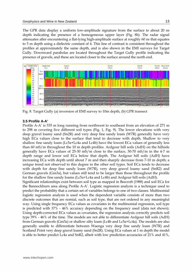
Soils are generally high in gravel content with gravels closest to the surface at the central-

north end. Clay content is less than 7% close to the surface, generally decreases with depth

and is largest at the north end close to the surface. Soil ECa values are similar throughout

the Target Gully profile at roughly 0-5 m depth (Fig. 8a). The lowest soil ECa values are in

the northern area of the block at depths of less than 5 m. There is a sharp increase in soil ECa

values at roughly 5 m depth throughout the length of the row. Soil ECa values generally

increase below this 5 m depth, and the largest values are in the south.

www.intechopen.com


13

The GPR data display a uniform low-amplitude signature from the surface to about 20 ns depth indicating the presence of a homogeneous upper layer (Fig. 8b). The radar signal attenuates after encountering a flat-lying high-amplitude surface at roughly 60 ns that equates to 5 m depth using a dielectric constant of 4. This line of contrast is consistent throughout the profiles at approximately the same depth, and is also shown in the EMI surveys for Target Gully. Downward parabolas are located throughout the Target Gully profile indicating the presence of gravels, and these are located closer to the surface around the north end.

Fig. 8. Target Gully (a) inversion of EMI survey to 10m depth, (b) GPR transect

3.5 Profile A-A’ Profile A-A’ is 535 m long running from northwest to southeast from an elevation of 271 m to 298 m covering five different soil types (Fig. 1, Fig. 9). The lower elevations with very deep gravel loamy sand (Sn2R) and very deep fine sandy loam (W7R) generally have very high ECa values close to the surface that tend to decrease with depth. Shallow to very shallow fine sandy loam (Lc5a+Lc4a and Lc4b) have the lowest ECa values of generally less than 60 mS/m throughout the 10 m depth profiles. Ardgour hill soils (AdH) on the hillside generally have ECa values of 25-30 mS/m close to the surface, 30-70 mS/m in the 4-7 m depth range and lower soil ECa below that depth. The Ardgour hill soils (AdH) have increasing ECa with depth until about 7 m and then sharply decrease from 7-10 m depth; a unique trend not observed to this degree in the other soil types. Soil ECa tends to decrease with depth for deep fine sandy loam (W7R), very deep gravel loamy sand (SnR2) and German gravels (Gm3a), but values still tend to be larger than those throughout the profile for the shallow fine sandy loams (Lc5a+Lc4a and Lc4b) and Ardgour hill soils (AdH). Significant relationships exist between soil type as mapped in Beecroft (1988) and soil ECa for the Bannockburn area along Profile A-A’. Logistic regression analysis is a technique used to predict the probability that a certain set of variables belongs to one of two classes. Multinomial logistic regression analysis is used when the dependent variable consists of more than two discrete outcomes that are nomial, such as soil type, that are not ordered in any meaningful way. Using single frequency ECa values as covariates in the multinomial regression, soil type is predicted with 37% - 46% accuracy depending on the frequency used (data not shown). Using depth-corrected ECa values as covariates, the regression analysis correctly predicts soil type 39% - 46% of the time. The models are not able to differentiate Ardgour hill soils (AdH) from German gravels (Gm3a) or shallow silty loam (Lc4b and Lc5a+Lc4a). The models are also generally unable to differentiate between Waenga very deep fine sandy loam (W7R) and Scotland Point very deep gravel loamy sand (Sn2R). Using ECa values at 1 m depth the model is able to better predict Lc4a and SnR2, albeit with low prediction accuracies of 21% and 41%,

www.intechopen.com


14

respectively. Using ECa values below 6 m depth results in an increased prediction accuracy for German gravels. The model predicts soil type with 38% accuracy when only ECa at 1 m and 2 m depths are used in the regression analysis (data not shown). Using depth-corrected multi-frequency ECa data in 1 m intervals in the model predicts soil type with 69.2% accuracy overall, showing the added benefit of using multi-frequency ECa data.

Fig. 9. Inversion of EMI survey to 10 m depth along Profile A-A'

3.6 Soil chemical analysis Fig. 10 shows selected representative soil nutrient data for one representative trench at each site. In order to account for the relative dearth of available nutrients in gravelly soils, these values are mass-balance corrected; nutrient concentrations are multiplied by the percentage of soil that is <2 mm.

Total N (%)

0

50

100

150

200

250

0 0.1 0.2 0.3 0.4

Dep

th (

cm)

Felton Road

Olssens

Target Gully

CEC

0

50

100

150

200

250

0 10 20

Dep

th (

cm)

Fig. 10. Soil profiles (left) and example nutrient profiles of Total N (%) and CEC

www.intechopen.com


15

Soil pH values tend to increase with depth at all sites and are largest at Felton Road. At 100 cm depth, the pH at Felton Road is approximately 8.5, and it is <7.0 at Target Gully. Shallow soil samples at all three sites have similar pH values. At Target Gully, Ca-rich layers occur in deeper soils. At Felton Road, Cu, Mg, K, N and Mn concentrations are typically greater throughout the soil profiles than at the other sites. Total CEC is largest at Felton Road throughout the soil profile, and is mainly comprised of 80% Ca at Felton Road, 73% Ca at Olssens and 70% Ca at Target Gully.

4. Discussion

4.1 Vine vigour Vine trunk circumferences can be used as an indicator of vine vigour (e.g. Clingeleffer & Emmanuelli, 2006; Acevedo-Opazo et al., 2008; Trought et al., 2008). In uniformly managed blocks where vine trunk circumferences vary little, the growing conditions within the block are considered to be more uniform. Conversely, where vine sizes show more variation, growing conditions are considered to be less uniform. Average vine trunk circumferences show variation at all study sites (Fig. 2). When examining the range of average values of vine trunk circumferences in individual bays within a study block, the largest value is up to 65% larger than the smallest value, even after the data were cleaned by removing the smallest vines. Although the study sites are managed slightly differently, management within each block is uniform and therefore other variables, including soil conditions, likely control vine sizes. Variations in grapevine vigour commonly correlate with fruit/wine characteristics on a site-specific level elsewhere (e.g. Cortell et al., 2005; Trought et al., 2008), so the variation in grapevine trunk circumference observed at these study sites likely contributes to differences in grape characteristics. Yield can vary up to 10-fold in the same vineyard block, and this variation in yield has associated quality implications (Bramley, 2001). Management practices such as differential harvesting based on vigour zones may lead to more consistency of fruit composition delivered to the winery (e.g. Proffitt et al., 2006). Felton Road had the largest vine trunk circumference values and largest vine trunk circumference growth per year. The soils at Felton Road are characterised by deep sandy to silty loams. In contrast, the Target Gully site is on soils that contain abundant schist fragments, and the Olssens site contains abundant gravels. The gravelly soils at Olssens and Target Gully produce vines with smaller trunk circumferences than the deep loams at Felton Road. Soil fertility indicators N, P and K are generally greater at Felton Road throughout the soil profile. Deep soils are more nutrient-rich at Felton Road than at the other two sites, even though similar concentrations are in the shallow samples. This may indicate that grapevines are able to extract nutrients from deep in the soil profile, and current vineyard management practices which generally test shallow soils only, may be overlooking this important variable. These deeper soil properties may also influence grape and wine characteristics, and are an often overlooked component of soil terroir. Some soils in this research were below recommended plant available nutrient concentrations for viticulture in New Zealand. The vines, however, did not show any obvious signs of nutrient deficiencies, presumably because they were able to extract nutrients from deep soils. More research determining plant uptake of deep nutrients is warranted, and a critical examination of recommended guidelines for viticulture in New Zealand should be undertaken.

www.intechopen.com


16

4.2 Geophysics and vine physiology In the GPR maps, areas of high and low amplitude signals are shown by dark and light patches, respectively. Areas of similar radar reflectance are an indication that the GPR is showing relative homogeneity in properties affecting radar reflectance at these sites. In this study, correlations vary between vine trunk circumferences and GPR data. In general, maps with distinct areas of high and low amplitude signals show visual correlations with vine trunk circumference data, but some study sites do not show much variability in GPR data. At Felton Road (Fig. 3), areas of high amplitude signals on the GPR map correlate with areas with smaller vine trunk circumferences, suggesting that soil properties that are less conducive to vine growth produce higher amplitude signals at this site. GPR surveys over the more gravelly soils at Olssens (Fig. 5) and Target Gully (Fig. 7) do not show distinct areas of high and low amplitude signals, and therefore radar reflectance data do not correlate well with vine trunk circumference data at these sites. Water has a high dielectric constant (k=80) when compared to common geological materials (k=5-15), and GPR field measurements are therefore largely a function of the available water in the soil (e.g. Galagdara et al. 2005). Therefore, GPR results at our study sites may be detecting changes in the available water content of different layers, rather than changes in the physical properties of the layers themselves. Nonetheless, differences in soil texture can be interpreted from water content maps (e.g. Hubbard et al., 2002; Grote et al., 2003), and future work at these study sites may improve our understanding of the causes of variability in GPR results at sites such as Felton Road. Relative soil ECa values alone do not provide an accurate prediction of grapevine trunk circumference variation; instead these correlations must be established on a site-by-site basis. Soil ECa values can be influenced by many different properties, including soil texture, clay content, soil extractable Ca2+, Mg2+, Na+, CEC, silt, salinity, organic matter, water content, and previous fertilizer application (e.g. Bronson et al., 2005; Corwin & Lesch, 2005). Zones of relatively high and low soil ECa are evident at Felton Road, and the areas with high soil ECa values tend to contain grapevines with relatively small vine trunk circumferences. These areas tend to have a greater silt and clay content at depth, whereas the areas with lower soil ECa values in the north of the block are derived from soils that have higher gravel contents. At Olssens, soils with relatively low ECa values in the north and south of the block tend to contain smaller vines. These areas are delineated with ECa maps showing areas of high and low soil ECa values. Maps created from GPR and EMI surveys have the potential to measure soil properties that can influence grapevine vigour. Grapevines at Felton Road, for example, tend to form distinct clusters of similar sized vines. The maps produced by the GPR and EMI surveys also clearly delineate areas of different radar reflectance and areas of high and low soil ECa. Using such survey methods can potentially delineate areas of soil properties that may influence vine growth.

4.3 Geophysics – GPR and multi-frequency EMI surveys Some similarities exist between aerial maps produced using the GPR and EMI data. The Felton Road surveys, for example, show similar patterns for both techniques in a large area of the study block. Areas of high amplitude signals in the GPR map are roughly cospatial with the higher soil ECa areas in the EMI map indicating soils with higher soil ECa also exhibit higher radar reflectance. Target Gully and Olssens have higher gravel content and tend to produce maps showing less distinct areas of variation making comparisons between

www.intechopen.com


17

the two techniques more difficult at these sites. Areas of high amplitude signals at Olssens are roughly cospatial with areas of both high and low soil ECa indicating different properties may influence these readings. Depth to soil texture contrasts can be estimated using GPR (e.g. Simeoni et al., 2009), and our work suggests that EMI surveys can also yield information that can help estimate depths to horizons where soil texture changes significantly. For example, the area around the Target Gully study site was subject to sluicing activity for alluvial gold, and the distinct contrasts in the GPR and EMI surveys at roughly 5 m depth may indicate the depth of the deposited sediment during the late 1800s to early 1900s. GPR is known to detect human induced disturbances, such as this sluice deposit, because of its sensitivity to the contrast between the natural and unnatural strata in the deposits which result in a strong high-amplitude reflection (Daniels, 2004). Depth penetration is lowest at this site for the EMI survey, possibly due to relatively recent increased sediment disturbance. Conducting a single-frequency EMI survey would likely not yield data suitable to measuring thickness of the deposited sediment. High soil ECa can cause the GPR signal to attenuate quickly and produce poor quality survey results (GSSI, 2004). The Felton Road GPR survey has a poor record in the middle of the transect. High soil ECa is measured by the EMI survey at the surface, and this alone does not attenuate the GPR signal at this site. Areas of high soil ECa with depth visually correlate to locations of impeded GPR signals in the middle of the Felton Road study row indicating that a thin layer of highly conductive soil close to the surface may not necessarily result in poor quality GPR imaging. The GPR quality is lowest at this site, possibly due to very high soil ECa values. Areas of high soil ECa that affect GPR survey quality may not be detrimental to multi-frequency EMI survey quality. When interpreting results from single-frequency EMI surveys, it is difficult to make an assessment of signal depth penetration, and consequently soil homogeneity or heterogeneity with depth is difficult to estimate. The EM38 and Veris-3100 are commonly used in soil apparent electrical conductivity mapping (e.g. Bramley, 2001; Liu et al., 2008). These methods can map soil ECa at two different depths, the EM38 in horizontal and vertical dipole mode can measure soil ECa at roughly 0-75 cm and 0-150 cm, respectively, and the Veris-3100 usually measures at 0-30 cm and 0-90 cm. These depths, however, can vary with different soil properties. Our results suggest that soil properties can vary in close proximity, and these variations can have associated effects on survey depth penetration. Soil ECa values at Olssens are typically less than 1 mS/m. Inversion algorithms used in multi-frequency EMI surveys may have difficulty calculating depth penetration where soil ECa values are very low. With such low ECa values, little additional information is gained on soil ECa changes with depth by inverting the EMI data, and the inversion algorithm may be unable to estimate depth penetration. Changes in soil ECa values with depth must be sufficient in order for multi-frequency EMI surveys to map these changes with reasonable precision. Soils with high clay content can decrease GPR survey quality, and increase EMI survey quality. High clay contents can produce high attenuation losses and can decrease GPR quality (Gerber et al., 2007), and our results are consistent with this observation. The north end of Target Gully contains 7.0% clay to roughly 40 cm depth, the largest in the row, and GPR quality is poor. Clay content in some Felton Road samples in the middle of the row is just less than 20%, and this location has both the largest depth-weighted percent clay and highest soil ECa with depth. The GPR signal exhibits attenuation loss to some degree where clay content is relatively large. Clay content has been positively correlated to ECa values (e.g. Hedley et al.

www.intechopen.com


18

2004), and this may be related to greater water holding capacity and typically larger water content than surrounding soils with less clay. The highest ECa values correspond to trenches with highest percent clay content at Felton Road. The EMI survey quality is not attenuated by high clay content at any of the sites, and shows good quality where clay content is highest and GPR survey quality is poor. Low clay content at Olssens may, in part, result in overall low ECa values at the site. Multi-frequency EMI surveys may be able to detect soil ECa changes, even below clay rich layers that are more impenetrable to GPR. Yoder et al. (2001) used EMI surveys to identify areas of high ECa, and then conducted GPR surveys to obtain more detailed information in these areas of interest. The results of this study indicate that multi-frequency EMI surveys may be able to replace the need for two surveys depending on the information required and providing that soil ECa differences with depth are sufficient. For example, the GPR survey is useful in indicating that to a depth of 5 m, Target Gully has less gravel and more uniform deposits than Olssens, which has more gravel and fluvial stratigraphy. At Target Gully, the contrast at 5 m depth is picked up by both GPR and EMI surveys. At the sites in this study, EMI survey quality was generally high providing soil ECa values are greater than roughly 1 mS/m. This demonstrates that multi-frequency EMI surveys can be used to estimate depth to layers of significant contrast within the subsurface. Different statistical techniques have been used to predict various soil properties from a

variety of data sources (e.g. James et al., 2003; McBratney et al., 2003 and references therein;

Liu et al., 2008; Grunwald, 2009). For example, logistic regression can be used to make

continuous soil maps of soil groups influenced by topography (Debella-Gilo & Etzelmüller,

2009) and to quantify relationships between ancillary variables and soil maps (Kempen et

al., 2009). The analysis presented here uses multinomial logistic regression to predict

mapped soil class using multi-frequency EMI data as covariates. No other studies were

found in the literature that use depth corrected ECa values as covariates in a statistical

regression analysis in an attempt to ascertain whether these data can predict soil type. Soil

ECa values with depth exhibit patterns for some mapped soil types (Fig. 9). An increase in

prediction accuracy from ~40% to 69% correct of the multinomial regression analysis occurs

when using depth corrected ECa values instead of single frequency values. Results of the

statistical analyses suggest that multi-frequency ECa data are better able to predict soil type

than single frequency data alone. This may in part be due to different trends observed in

ECa with depth for different soil types.

4.4 Applications in precision viticulture – Geophysics and wine Precision agriculture incorporates widespread use of technologies that give valuable information about soil variation. Precision agriculture is beneficial in many different industries, and Bramley (2009) provides an excellent review. Mapping the variability of soil is a key component of implementing precision agriculture, and various soil characteristics can be measured. Spatial variability in soils can be reflected in EMI surveys, which in turn can be useful for delineating areas for soil sampling (e.g. Bramley, 2003) or defining water restriction zones on a vineyard scale (e.g. Acevedo-Opazo et al., 2008). Another method that can be used in vineyards is normalised difference vegetation index (NDVI; Rouse et al., 1973) imaging, although if the goal is to measure vine canopy as opposed to soil properties, spatial resolutions of 20 cm are required to differentiate vine rows from cover crop (Lamb et al., 2001). The implementation of precision viticulture can be profitable; applications in

www.intechopen.com


19

Australia have shown a benefit of $30,000 - $40,000 / ha in some more extreme cases (Bramley 2009, and references therein). Vine trunk circumferences vary significantly within each of our study sites. Grape quality

has been linked to changes in vine vigour elsewhere (e.g. Bramley, 2003; Trought et al.,

2008), and therefore grapes with different characteristics are likely produced within our

sites. The EMI maps from our sites indicate that properties that affect soil conductivity may

also affect vine trunk circumference growth. Electromagnetic induction surveys, which

show local differences in soil apparent electrical conductivity, may provide valuable and

cost-effective inputs into precision management decisions for the New Zealand viticulture

industry, and these geophysical surveys should be accompanied by differential GPS surveys

that can be conducted concurrently to precisely map elevation, slope and aspect.

4.5 Future research The EMI sensor used for this research was the GEM-2 portable broadband electromagnetic sensor capable of measuring soil ECa up to roughly 48,000 Hz. The next generation GEM-2 is capable of measuring soil ECa up to roughly 96,000 Hz. The higher frequency capability measures ECa closer to the surface than the GEM-2 used in this research. By conducting multi-frequency surveys using higher frequencies, more detailed ECa profiles of the shallow soils can potentially be created. Conducting these surveys and inverting these data warrants further investigation, and may provide more precise data on soil ECa variability in soils in the rootzone. Further research in other New Zealand winegrowing regions should be conducted using the GEM-2 analysing depth penetration to test whether this survey method can be used in other soil types in New Zealand. Our research indicates that maps produced from EMI survey data show useful correlations with vine trunk circumference data, and we recommend continued uptake of these types of surveys by the agricultural industry (e.g. Bramley, 2009 and references therein). Closer integration with yield data and data that reflect fruit characteristics and ripeness could lead to refined management of individual vineyard blocks. Such geophysical surveys can also be beneficial in the early stages of vineyard block design, where blocks are delineated according to similar environmental parameters. The complex interactions between soil properties, grapevine physiology and must/wine properties are poorly understood. Wines from some regions, both internationally and in New Zealand, have similar characteristics leading some to assume soil imparts particular characteristics in wines. Soils are complex systems, and a wide variety of properties that may affect grape compounds can be further researched. Microvinification research should be conducted on a vineyard block scale comparing soil and wine properties in close proximity in order to determine if soil variability between adjacent grapevines influences wine properties. The lack of data that specifically links soil properties and wine characteristics indicates that far more research is required in this area. A better understanding of how soil influences specific wine properties will enhance winemakers’ abilities to produce wines of desired flavour and aroma profiles.

5. Conclusions

Ground penetrating radar and electromagnetic induction surveys have the potential to be used as inputs for precision viticulture, and our results indicate that in New Zealand, both techniques can provide useful results. A wide variety of factors can affect the results of these

www.intechopen.com


20

surveys, and additional work is needed in New Zealand and elsewhere to help constrain the relative influences of different attributes on geophysical data and how these attributes influence vine growth and grape characteristics. Nonetheless, our results show that EMI surveys provide data that more clearly correlate with variations in vine trunk circumference data than GPR surveys, and including topography in such analyses may prove beneficial. As GPR surveys are also more expensive and time consuming, EMI surveys are the preferred tool for defining variation in soils in New Zealand. Multi-frequency EMI surveys can also be used to map areas of different soil type more effectively than more traditional single-frequency surveys. Environmental properties such as slope, aspect, elevation, growing degree days and sunshine hours are similar at three adjacent vineyards in Bannockburn, Central Otago. Viticultural management practices such as trellis design, fruit exposure and bunches per shoot between these sites are also similar. However, the three sites have significantly different soils with different physical and chemical properties, and the vine trunk circumferences vary significantly among these sites. The soil component of terroir can have a significant impact on vine characteristics, and presumably also on grape and wine properties. Geophysical survey methods can provide insight into both horizontal and vertical changes in soil variability, and these data can be used to quantify and better understand physical and chemical properties of soils that affect grape and wine properties. A more comprehensive reference list and complete information on the research presented in this chapter can be accessed at https://researchspace.auckland.ac.nz/handle/2292/6141 (Imre 2011).

6. References

Acevedo-Opazo, C., Tisseyre, B., Guillaume, S. and Ojeda, H., 2008, The potential of high spatial resolution information to define within-vineyard zones related to vine water status: Precision Agriculture, v. 9, p. 285-302.

Beecroft, F.G., 1988, Soil taxonomic unit descriptions for Bannockburn Valley, Central Otago, South Island, New Zealand: NZ Soil Bureau, Department of Scientific and Industrial Research, Wellington, 174 p.

Bramley, R.G.V., 2001, Progress in the development of precision viticulture - Variation in yield, quality and soil properties in contrasting Australian vineyards, in Currie, L.D. and Loganathan, P., eds, Precision tools for improving land management: Occasional report No. 14, Fertilizer and Lime Research Centre, Massey University, Palmerston North. P. 25-43.

Bramley, R., 2003, Smarter thinking on soil survey: Australian and New Zealand wine industry journal, v. 18(3), p. 88-94.

Bramley, R.G.V., 2009, Lessons from nearly 20 years of precision agriculture research, development, and adoption as a guide to its appropriate application: Crop and Pasture Science, v. 60, p. 197-217.

Bravdo, B.A., 2001, Effect of Cultural Practices and Environmental Factors on Fruit and Wine quality: Agriculturae Conspectus Scientificus, v. 66 (1), p. 13-20

Bronson, K.F., Booker, J.D., Officer, S.J., Lascano, R.J., Maas, S.J., Searcy, S.W., and Booker, J., 2005, Apparent electrical conductivity, soil properties and spatial covariance in the U.S. Southern High Plains: Precision Agriculture, v. 6, p. 297-311.

Carroll, Z.L. and Oliver, M.A., 2005, Exploring the spatial relations between soil physical properties and apparent electrical conductivity: Geoderma, v. 128, p. 354-374.

www.intechopen.com


21

Clingeleffer, P.R. and Emmanuelli, D.R., 2006, An assessment of rootstocks for Sunmuscat (Vitis vinifera L.): a new drying variety: Australian Journal of Grape and Wine Research, v. 12, p. 135-140.

Cockx, L., van Meirvenne, M. and De Vos, B., 2007, Using the EM38DD soil sensor to delineate clay lenses in a sandy forest soil: Soil Science Society of America Journal, v. 71, p. 1314-1322.

Cortell, J.M., Halbleib, M., Gallagher, A.V., Righetti, T.L. and Kennedy, J.A., 2005, Influence of vine vigor on grape (Vitis Vinifera L. Cv. Pinot Noir) and wine proanthocyanidins: Journal of Agricultural and Food Chemistry, v. 53, p. 5798-5808.

Cortell, J.M. and Kennedy, J.A., 2006, Effect of shading on accumulation of flavonoid compounds in (Vitis Vinifera L.) Pinot Noir fruit and extraction in a model system: Journal of Agricultural and Food Chemistry, v. 54, p. 8510-8520.

Corwin, D.L., and Lesch, S. M., 2005, Apparent soil electrical conductivity measurements in agriculture: Computers and Electronics in Agriculture, v. 46, p. 11-43.

Daniels, D.J., 2004, Ground Penetrating Radar 2nd Edition: IEE Radar, Sonar and Navigation series 15: Institution of Electrical Engineers, London, 726 p.

De Andres-de Prado, R., Yuste-Rojas, M., Sort, X., Andres-Lacueva, C., Torres, M. and Lamuela-Raventos, R.M., 2007, Effect of Soil Type on Wines Produced from Vitis vinifera L. Cv. Grenache in Commercial Vineyards: Journal of Agricultural and Food Chemistry 55 (3): 779-786.

Debella-Gilo, M. and Etzelmüller, B., 2009, Spatial prediction of soil classes using digital terrain analysis and multinomial logistic regression modeling integrated in GIS: Examples from Vestfold County, Norway: Catena, v. 77, p. 8-18.

Doolittle, J.A., Indorante, S.J., Potter, D.K., Hefner, S.G. and McCauley, W.M., 2002, Comparing three geophysical tools for locating sand blows in alluvial soils of southeast Missouri: Journal of Soil and Water Conservation, v. 57:3, p. 175-182.

Dry, P.R. and Loveys, B.R., 1998, Factors influencing grapevine vigour and the potential for control with partial rootzone drying: Australian Journal of Grape and Wine Research, v. 4(3), p. 140-148.

Eckert, D. and Sims, J.T., 1995, Recommended soil pH and lime requirement tests, in Sims, J.T., and Wolf, A. eds, Recommended Soil Testing Procedures for the Northeastern United States. Northeast Regional Bulletin #493, Agricultural Experiment Station, University of Delaware, Newark, DE, USA, p.11-16.

Galagdara, L.W., Parkin, G.W., Redman, J.D., von Bertoldi, P., and Endres, A.L., 2005, Field studies of the GPR ground wave method for estimating soil water content during irrigation and drainage: Journal of Hydrology, v. 301, p. 182-197.

Galet, P., 2000, General Viticulture. Translated by John Towey. Oenoplurimédia. France, 443 p. Gerber, R., Salat, C., Junge, A. and Felix-Henningsen, P., 2007, GPR-based detection of

Pleistocene periglacial slope deposits at a shallow-depth test site: Geoderma, v. 139, p. 346-356.

Gómez-Míguez, M.J., Gómez-Míguez, M., Vicario, I.M. and Heredia, F.J., 2007, Assessment of colour and aroma in white wines vinifications: Effects of grape maturity and soil type: Journal of Food Engineering, v. 79: p. 758-764.

Grote, K., Hubbard, S., and Rubin, Y., 2003, Field-scale estimation of volumetric water content using GPR groundwave techniques: Water Resources Research, v. 39-11, p. SBH5.1-5-SBH5.13.

Grunwald, S., 2009, Multi-criteria characterization of recent digital soil mapping and modelling approaches: Geoderma, v. 152, p. 195-207.

www.intechopen.com


22

GSSI (Geophysical Survey Systems, Inc.), 2004, RADAN 6 User’s Manual: Geophysical Survey Systems, Inc. United States, 135 p.

Haeger, J.W., 2004, North American Pinot Noir: University of California Press, Berkley. 445 p. Hartsock, N.J., Mueller, T.G., Thomas, G.W., Barnhisel, R.I., Wells, K.L. and Shearer, S.A.,

2000, Soil Electrical Conductivity Variability, in Robert P.C., et al. eds, Proc. 5th international conference on precision Agriculture, ASA Misc. Publ., ASA, CSSA, and SSSA, Madison, WI.

Hedley, C.B., Yule, I.J., Eastwood, C.R., Shepherd, T.G. and Arnold, G., 2004, Rapid identification of soil textural and management zones using electromagnetic induction sensing of soils: Australian Journal of Soil Research, v. 42, p. 389-400.

Huang, H., 2005, Depth of investigation for small broadband electromagnetic sensors: Geophysics, v. 70, p. G135-G142.

Huang, H., and Won, I.J., 2003, Real-time resistivity soundings using a hand-held broadband electromagnetic sensor: Geophysics, v. 68, p. 1224-1231.

Hubbard, S., Grote, K. and Rubin, Y., 2002, Mapping the volumetric soil water content of a California vineyard using high-frequency GPR ground wave data: The Leading Edge, June, p. 552-559.

Iland, P., 2004, Chemical analysis of grapes and wine: techniques and concepts. Campbelltown, SA, Australia, Patrick Iland Wine Promotions PTY LTD.

Imre, S.P., 2011, A Multi-disciplinary study to quantify terroir in Central Otago and Waipara Pinot Noir vineyards. PhD thesis, University of Auckland, New Zealand.

Imre, S.P. and Mauk, J.L. 2009, New Zealand Terroir: Geoscience Canada, v. 36(4), p. 145-159. Imre, S.P., Mauk, J.L., Bell, S. and Dougherty, A., 2009a, Correlations among ground

penetrating radar, electromagnetic induction and vine trunk circumference data: towards quantifying terroir in New Zealand Pinot Noir vineyards: Le Progrès agricole et viticole, ISSN 0369-8173, v. 126 (1), p. 8-11.

Imre, S.P., Mauk, J.L., Bell, S., and Dougherty, A., 2009b, Mapping grapevine vigour and lateral variation in soils: Journal of Wine Research, Submitted Dec 2009.

Jackson, D.I. and Lombard, P.B., 1993, Environmental and Management Practices Affecting Grape Composition and Wine Quality - A Review: American Journal of Enology and Viticulture, v. 44 (4), p. 409-430

Jackson, R., 1994, Wine science: principles and applications. Oxford, UK. Elsevier Inc., 751 p. James, I.T., Waine, T.W., Bradley, R.I., Taylor, J.C. and Godwin, R.J., 2003, Determination of

soil type boundaries using electromagnetic induction scanning techniques: Biosystems Engineering, v. 86:4, p. 421-430.

Jol, H.M., 2009, Ground Penetrating Radar: Theory and Applications. Elsevier 544 p. Keller, M., 2005, Deficit Irrigation and Vine Mineral Nutrition: American Journal of Enology

and Viticulture, v. 56 (3), p. 267-283. Kempen, B., Brus, D.J., Heuvelink, G.B.M. and Stoorvogel, J.J., 2009, Updating the 1:50,000

Dutch soil map using legacy soil data: A multinomial logistic regression approach: Geoderma, v. 151, p. 311-326.

Kitchen, N.R., Sudduth, K.A. and Drummond, S.T., 1996, Mapping of sand deposition from 1993 midwest floods with electromagnetic induction measurements: Journal of Soil and Water Conservation, v. 51:4, p. 336-340.

Lamb, D., Hall, A. and Louis, J., 2001, Airborne remote sensing of grapevines for canopy variability and productivity. The Australian Grapegrower and Winemaker, v. 449a, 89–92.

Lambert, J.J., Dahlgren, R.A., Battany, M., McElrone, A. and Wolpert, J.A., 2008, Impact of soil properties on nutrient availability and fruit and wine characteristics in a Paso

www.intechopen.com


23

Robles vineyard. Proceedings of the 2nd Annual National Viticulture Research Conference. July 9-11, 2008. University of California, Davis. p. 44-45.

Leathwick, J., Morgan, F., Wilson, G., Rutledge, D., McLeod, M., and Johnston, K., 2002, Land environments of New Zealand: A Technical Guide: David Bateman Ltd., Auckland, 237 p.

Liu, J., Pattey, E., Nolin, M.C., Miller, J.R. and Ka, O., 2008, Mapping within-field soil drainage using remote sensing, DEM and apparent soil electrical conductivity: Geoderma, v. 143, p. 261-262.

Mackenzie, D.E. and Christy, A.G., 2005, The role of soil chemistry in wine grape quality and sustainable soil management in vineyards: Water Science and Technology, v. 51 (1), p. 27-37.

Macqueen, R.W., and Meinert, L.D., eds., 2006, Fine wine and terroir: the geoscience perspective: Geological Association of Canada, St John’s Newfoundland, Canada, 247 p.

McBratney, A.B., Mendonça Santos, M.L. and Minasny, B., 2003, On digital soil mapping: Geoderma, v. 117, p. 3-52.

New Zealand Winegrowers, 2009, Annual Report: http://nzwine.com/intro/. 20 p. NZIER, 2009, Economic impact of the New Zealand wine industry. www.nzier.org.nz:

Wellington, New Zealand, 32 p. OIV (Organisation Internationale de la Vigne et du Vin), 2006, Situation of the world

viticulture sector in 2006, http://news.reseauconcept.net/images/oiv_uk/client/Commentaire_statistiques_

annexes_2006_EN.pdf Ojeda, H., Andary, C., Kraeva, E., Carbonneau, A. and Deloire, A., 2002, Influence of Pre-

and Postveraison Water Deficit on Synthesis and Concentration of Skin Phenolic Compounds during Berry Growth of Vitis vinifera cv. Shiraz: American Journal of Enology and Viticulture, v. 53 (4), p. 261-267.

Oliveira, C., Silva Ferreira, A.C., Mendes Pinto, M., Hogg, T., Alves, F. and Guedes de Pinho, P., 2003, Carotenoid Compounds in Grapes and Their Relationship to Plant Water Status: Journal of Agricultural and Food Chemistry, v. 51 (20), p. 5967-5971.

Peyrot des Gachons, C., van Leeuwen, C., Tominaga, T., Soyer, S., Gaudillegrave, J. and Dubourdieu, D., 2005, Influence of water and nitrogen deficit on fruit ripening and aroma potential of Vitis vinifera L cv Sauvignon blanc in field conditions: Journal of the Science of Food and Agriculture, v. 85, p. 73-85.

Proffitt, T., Bramley, R., Lamb, D. and Winter E., 2006, Precision viticulture – A new era in vineyard management and wine production: Winetitles: Adelaide. 92. p.

Ross, D., 1995, Recommended soil tests for determining soil cation exchange capacity, in Sims, J.T., and Wolf, A. eds., Recommended Soil Testing Procedures for the Northeastern United States. Northeast Regional Bulletin #493. Agricultural Experiment Station, University of Delaware, Newark, DE, USA., p.62-69.

Rouse, J.W., Haas, R.H., Schell, J.A. and Deering, D.W., 1973, Monitoring vegetation systems in the Great Plains with ERTS. In ‘Proceedings of the 3rd ERTS Symposium’ NASA SP351, 1. p, 309-317. US Government Printing Office: USA)

Sabon, I., de Revel, G., Kotseridis, Y. and Bertrand, A., 2002., Determination of Volatile Compounds in Grenache Wines in Relation with Different Terroirs in the Rhone Valley: Journal of Agricultural and Food Chemistry, v. 50 (22), p. 6341-6345.

Sarneckis, C.J., Dambergs, R.G., Jones, P., Mercurio, M., Herderich, M.J. and Smith, P.A., 2006, Quantification of condensed tannins by precipitation with methyl cellulose:

www.intechopen.com


24

development and validation of an optimised tool for grape and wine analysis: Australian Journal of Grape and Wine Research, v. 12 (1), p. 39-49.

Simeoni, M.A., Galloway, P.D., O’Neil, A.J. and Gilkes, R.J., 2009, A procedure for mapping the depth to the texture contrast horizon of duplex soils in south-western Australia using ground penetrating radar, GPS and kriging: Australian Journal of Soil Research, v. 47, p. 613-621.

Smart D.R, Schwass, E., Lakso, A., Morano, L., 2006, Grapevine rooting patterns: a comprehensive analysis and review: American Journal of Enology and Viticulture, v. 57:1, p. 89-104.

Swinchatt, J. and Howell, D.G., 2004, The Winemaker’s Dance: Exploring terroir in the Napa Valley: University of California Press, Berkley. 229 p.

Tominaga, T., Murat, M.L. and Dubourdieu, D., 1998, Development of a method for analyzing the volatile thiols involved in the characteristics aroma of wine made from Vitis vinifera L. cv. Sauvignon blanc: Journal of Agricultural and Food Chemistry, v. 46 (3), p. 1044-1048.

Trought, M. C. T., Dixon, R., Mills, T., Greven, M., Agnew, R., Mauk, J. L., and Praat, J.-P., 2008, The impact of differences in soil texture within a vineyard on vine vigour, vine earliness and juice composition: Journal International des Sciences de la Vigne et du Vin, v. 42 (2), p. 67–72.

Turnbull, I.M. (compiler), 2000, Geology of the Wakitipu area. Institute of Geological & Nuclear Sciences 1:250 000 geological map 18. 1 sheet + 72 p. Lower Hutt, New Zealand. Institute of Geological and Nuclear Sciences Limited.

USEPA, 1986, Test methods for evaluating solid waste. Volume IA: 3rd Edition, EPA/SW-846. National Information Service. Springfield, VA, USA.

Van Leeuwen, C., Friant, P., Choné, X., Trégoat, O., Koundouras, S. and Dubourdieu, D., 2004, Influence of climate, soil, and cultivar on terroir: American Journal of Enology and Viticulture, v. 55 (3), p. 207–217.

White, R. 2003. Soils for fine wines. Oxford University Press Inc. New York. 279 p. White, R., Balachandra, L., Edis, R. and Chen, D., 2007, The soil component of terroir:

Journal International des Science de la Vigne et du Vin, v. 41, p. 9-18. Wilson, J.E., 1998, Terroir: The role of geology, climate, and culture in the making of French

wines: University of California Press, Berkley. 336 p. Winkler, A.J., Cook, J.A., Kliewer, W.M. and Lider, L.A., 1962. General Viticulture.

University of California Press, USA, 710 p. Wolf, A.M. and Beegle, D.B., 1995, Recommended soil tests for macronutrients: phosphorus,

potassium, calcium, and magnesium, in Sims J.T., and Wolf A., eds., Recommended Soil Testing Procedures for the Northeastern United States. Northeast Regional Bulletin #493, Agricultural Experiment Station, University of Delaware, Newark, DE, USA, p. 25-34.

Won, I.J., Keiswetter, D.A., Fields, G.R.A., and Sutton, L.C., 1996, GEM-2: A New Multifrequency Electromagnetic Sensor: Journal of Environmental and Engineering Geophysics, v. 1:2, p. 129-137.

Yoder, R.E. Freeland, R.S., Ammons, J.T. and Leonard, L.L., 2001, Mapping agricultural fields with GPR and EMI to identify offsite movement of agrochemicals: Journal of Applied Geophysics, v. 47, p. 251-259.

Zou, H., Kilmartin, P., Inglis, M. and Frost, A., 2002, Extraction of phenolic compounds during vinification of Pinot Noir wine examined by HPLC and cyclic voltammetry: Australian Journal of Grape and Wine Research, v. 8 (3), p. 163-174.

www.intechopen.com

Earth and Environmental SciencesEdited by Dr. Imran Ahmad Dar

ISBN 978-953-307-468-9Hard cover, 630 pagesPublisher InTechPublished online 07, December, 2011Published in print edition December, 2011

InTech EuropeUniversity Campus STeP Ri Slavka Krautzeka 83/A 51000 Rijeka, Croatia Phone: +385 (51) 770 447 Fax: +385 (51) 686 166www.intechopen.com

InTech ChinaUnit 405, Office Block, Hotel Equatorial Shanghai No.65, Yan An Road (West), Shanghai, 200040, China

Phone: +86-21-62489820 Fax: +86-21-62489821

We are increasingly faced with environmental problems and required to make important decisions. In manycases an understanding of one or more geologic processes is essential to finding the appropriate solution.Earth and Environmental Sciences are by their very nature a dynamic field in which new issues continue toarise and old ones often evolve. The principal aim of this book is to present the reader with a broad overviewof Earth and Environmental Sciences. Hopefully, this recent research will provide the reader with a usefulfoundation for discussing and evaluating specific environmental issues, as well as for developing ideas forproblem solving. The book has been divided into nine sections; Geology, Geochemistry, Seismology,Hydrology, Hydrogeology, Mineralogy, Soil, Remote Sensing and Environmental Sciences.

How to referenceIn order to correctly reference this scholarly work, feel free to copy and paste the following:

Stephen P. Imre and Jeffrey L. Mauk (2011). Geophysics and Wine in New Zealand, Earth and EnvironmentalSciences, Dr. Imran Ahmad Dar (Ed.), ISBN: 978-953-307-468-9, InTech, Available from:http://www.intechopen.com/books/earth-and-environmental-sciences/geophysics-and-wine-in-new-zealand

geophysics and wine in new zealand -...

Documents