geophysics field camp 2014 - colorado school of mines · 2019-08-31 · geophysics field camp 2014...
TRANSCRIPT


Geophysics Field Camp 2014
Geophysical Investigation of the Chromo, COGeothermal System
Colorado School of Mines
June 6, 2014
Abstract
We examine the geothermal system in Chromo, Archuleta County, Colorado, using a widevariety of geophysical methods as part of the 2014 Colorado School of Mines Departmentof Geophysics’ summer field camp. With the goal of understanding geothermal fluid flowpathways in the area, we expanded on characterization of the Archuleta Arch, an anticlinalfeature and the dominant geological structure in the region. From May 12th to May 22nd,we collected survey, geology, deep seismic, shallow seismic, ground penetrating radar, D.C.resistivity, self-potential, time-domain electromagnetics, magnetotellurics, gravity and mag-netics data along a nine kilometer stretch of county road 382 in Chromo. An additionalsurvey was designed and collected by our student team using a variety of near-surface tech-niques in order to model the response of corroded well casings in Crowley Ranch. The use ofproper field acquisition techniques were a primary goal of the acquisition process. Followingthe time in the field, we analyzed, processed, and interpreted the data using relevant soft-ware for each individual method. Results were integrated and processed jointly to assist ininterpretation of fluid flow in the region.
Results from our Main Line suggest the presence of a large thrust fault along the crestof the anticline structure, with an estimated 700-1000 meters of throw. Our seismic, gravity,magnetotellurics and geologic information all support the thrust fault structure. Addition-ally, we locate the presence of a normal faulted fracture zone extending to the near surfacebelow the Stinking Springs. Electromagnetic and DC resistivity data support the fracturezone model as a zone of increased conductivity and fluid flow. We demonstrate the viabilityof a large thrust fault through the reactivation of a older, smaller reverse fault during thefolding of the anticline structure in the Laramide Orogeny. The presence of a large thrustfault in addition to a fracture zone underneath known surface expressions of geothermalwater provide pathways for hot water to reach the surface in the Chromo region. We expandthe geothermal flow model of the entire region, suggesting the transport of geothermal waterthrough the fractured crystalline basement rock connecting Chromo and the north-west townof Pagosa Springs.
Results from our Student Site indicate the signature of corroded well casings can be mod-eled using geophysical techniques. However the exact depth of well casings was unable tobe determined due to large cultural noise. We recommend procedures for improving dataquality and locating similar well casings in other area.
While our surveys detail a plausible explanation for geothermal fluid flow in the Chromo area,recommendations for additional characterization of the larger Archuleta County geothermalsetting are provided, as numerous questions about the fluid flow pathways still remain.

CONTENTS
1 Introduction 181.1 Background Information . . . . . . . . . . . . . . . . . . . . . . . . . . . . . 181.2 Objectives . . . . . . . . . . . . . . . . . . . . . . . . . . . . . . . . . . . . . 20
2 Geology 212.1 Geologic History . . . . . . . . . . . . . . . . . . . . . . . . . . . . . . . . . 21
2.1.1 Subsurface Geology . . . . . . . . . . . . . . . . . . . . . . . . . . . . 212.1.2 Surface Geology . . . . . . . . . . . . . . . . . . . . . . . . . . . . . . 23
2.2 Structural Geology . . . . . . . . . . . . . . . . . . . . . . . . . . . . . . . . 242.2.1 Regional Structural Features . . . . . . . . . . . . . . . . . . . . . . . 242.2.2 Local Structural Features . . . . . . . . . . . . . . . . . . . . . . . . 25
2.3 Field Observations . . . . . . . . . . . . . . . . . . . . . . . . . . . . . . . . 272.4 Geothermal Source . . . . . . . . . . . . . . . . . . . . . . . . . . . . . . . . 282.5 Hydrology . . . . . . . . . . . . . . . . . . . . . . . . . . . . . . . . . . . . . 28
3 Geophysics 293.1 Active vs. Passive Source . . . . . . . . . . . . . . . . . . . . . . . . . . . . . 293.2 Depth of Investigation . . . . . . . . . . . . . . . . . . . . . . . . . . . . . . 293.3 Modeling Techniques . . . . . . . . . . . . . . . . . . . . . . . . . . . . . . . 29
3.3.1 Forward Modeling . . . . . . . . . . . . . . . . . . . . . . . . . . . . 303.3.2 Inverse Modeling . . . . . . . . . . . . . . . . . . . . . . . . . . . . . 30
3.4 Survey . . . . . . . . . . . . . . . . . . . . . . . . . . . . . . . . . . . . . . . 313.4.1 Introduction . . . . . . . . . . . . . . . . . . . . . . . . . . . . . . . . 313.4.2 Background/Theory . . . . . . . . . . . . . . . . . . . . . . . . . . . 313.4.3 Differential GPS . . . . . . . . . . . . . . . . . . . . . . . . . . . . . 313.4.4 Handheld GPS . . . . . . . . . . . . . . . . . . . . . . . . . . . . . . 323.4.5 GPS used with Geophysical Methods . . . . . . . . . . . . . . . . . . 333.4.6 ArcMap . . . . . . . . . . . . . . . . . . . . . . . . . . . . . . . . . . 343.4.7 Survey Locations . . . . . . . . . . . . . . . . . . . . . . . . . . . . . 34
3.5 Gravity . . . . . . . . . . . . . . . . . . . . . . . . . . . . . . . . . . . . . . 353.5.1 Introduction . . . . . . . . . . . . . . . . . . . . . . . . . . . . . . . . 353.5.2 Background/Theory . . . . . . . . . . . . . . . . . . . . . . . . . . . 35
3.6 Magnetics . . . . . . . . . . . . . . . . . . . . . . . . . . . . . . . . . . . . . 37
2

CONTENTS
3.6.1 Introduction . . . . . . . . . . . . . . . . . . . . . . . . . . . . . . . . 373.6.2 Background/Theory . . . . . . . . . . . . . . . . . . . . . . . . . . . 38
3.7 Self-Potential . . . . . . . . . . . . . . . . . . . . . . . . . . . . . . . . . . . 413.7.1 Introduction . . . . . . . . . . . . . . . . . . . . . . . . . . . . . . . . 413.7.2 Background/Theory . . . . . . . . . . . . . . . . . . . . . . . . . . . 41
3.8 Direct Current Resistivity . . . . . . . . . . . . . . . . . . . . . . . . . . . . 433.8.1 Introduction . . . . . . . . . . . . . . . . . . . . . . . . . . . . . . . . 433.8.2 Background/Theory . . . . . . . . . . . . . . . . . . . . . . . . . . . 44
3.9 Electromagnetics . . . . . . . . . . . . . . . . . . . . . . . . . . . . . . . . . 463.9.1 Introduction . . . . . . . . . . . . . . . . . . . . . . . . . . . . . . . . 463.9.2 Background/Theory . . . . . . . . . . . . . . . . . . . . . . . . . . . 46
3.10 Magnetotellurics . . . . . . . . . . . . . . . . . . . . . . . . . . . . . . . . . 503.10.1 Introduction . . . . . . . . . . . . . . . . . . . . . . . . . . . . . . . . 503.10.2 Background/Theory . . . . . . . . . . . . . . . . . . . . . . . . . . . 50
3.11 Ground Penetrating Radar . . . . . . . . . . . . . . . . . . . . . . . . . . . . 523.11.1 Introduction . . . . . . . . . . . . . . . . . . . . . . . . . . . . . . . . 523.11.2 Background/Theory . . . . . . . . . . . . . . . . . . . . . . . . . . . 52
3.12 Hammer Seismic . . . . . . . . . . . . . . . . . . . . . . . . . . . . . . . . . 553.12.1 Introduction . . . . . . . . . . . . . . . . . . . . . . . . . . . . . . . . 553.12.2 Background/Theory . . . . . . . . . . . . . . . . . . . . . . . . . . . 55
3.13 Deep Seismic . . . . . . . . . . . . . . . . . . . . . . . . . . . . . . . . . . . 583.13.1 Introduction . . . . . . . . . . . . . . . . . . . . . . . . . . . . . . . . 583.13.2 Background/Theory . . . . . . . . . . . . . . . . . . . . . . . . . . . 59
4 Main Line 604.1 Gravity . . . . . . . . . . . . . . . . . . . . . . . . . . . . . . . . . . . . . . 60
4.1.1 Survey Location . . . . . . . . . . . . . . . . . . . . . . . . . . . . . . 604.1.2 Survey Design . . . . . . . . . . . . . . . . . . . . . . . . . . . . . . . 61
4.2 Processing . . . . . . . . . . . . . . . . . . . . . . . . . . . . . . . . . . . . . 614.2.1 Corrections . . . . . . . . . . . . . . . . . . . . . . . . . . . . . . . . 614.2.2 Modeling . . . . . . . . . . . . . . . . . . . . . . . . . . . . . . . . . 63
4.3 Interpretation/Discussion . . . . . . . . . . . . . . . . . . . . . . . . . . . . . 674.4 Sources of Error/Uncertainty . . . . . . . . . . . . . . . . . . . . . . . . . . 674.5 Conclusion . . . . . . . . . . . . . . . . . . . . . . . . . . . . . . . . . . . . . 684.6 Magnetics . . . . . . . . . . . . . . . . . . . . . . . . . . . . . . . . . . . . . 69
4.6.1 Survey Location . . . . . . . . . . . . . . . . . . . . . . . . . . . . . . 694.6.2 Survey Design . . . . . . . . . . . . . . . . . . . . . . . . . . . . . . . 694.6.3 Processing . . . . . . . . . . . . . . . . . . . . . . . . . . . . . . . . . 704.6.4 Interpretation . . . . . . . . . . . . . . . . . . . . . . . . . . . . . . . 724.6.5 Sources of Error/Uncertainty . . . . . . . . . . . . . . . . . . . . . . 744.6.6 Conclusion . . . . . . . . . . . . . . . . . . . . . . . . . . . . . . . . . 74
4.7 Direct Current Resistivity . . . . . . . . . . . . . . . . . . . . . . . . . . . . 754.7.1 Survey Location . . . . . . . . . . . . . . . . . . . . . . . . . . . . . . 754.7.2 Survey Design . . . . . . . . . . . . . . . . . . . . . . . . . . . . . . . 754.7.3 Processing . . . . . . . . . . . . . . . . . . . . . . . . . . . . . . . . . 794.7.4 Results . . . . . . . . . . . . . . . . . . . . . . . . . . . . . . . . . . . 834.7.5 Interpretation . . . . . . . . . . . . . . . . . . . . . . . . . . . . . . . 84
3

CONTENTS
4.7.6 Sources of Error/Uncertainty . . . . . . . . . . . . . . . . . . . . . . 844.7.7 Conclusion . . . . . . . . . . . . . . . . . . . . . . . . . . . . . . . . . 85
4.8 EM . . . . . . . . . . . . . . . . . . . . . . . . . . . . . . . . . . . . . . . . . 864.8.1 Survey Location: Main Line . . . . . . . . . . . . . . . . . . . . . . . 864.8.2 Survey Design . . . . . . . . . . . . . . . . . . . . . . . . . . . . . . . 864.8.3 Processing . . . . . . . . . . . . . . . . . . . . . . . . . . . . . . . . . 884.8.4 Interpretation . . . . . . . . . . . . . . . . . . . . . . . . . . . . . . . 924.8.5 Sources of Error/Uncertainty . . . . . . . . . . . . . . . . . . . . . . 934.8.6 Conclusion . . . . . . . . . . . . . . . . . . . . . . . . . . . . . . . . . 94
4.9 Magnetotellurics . . . . . . . . . . . . . . . . . . . . . . . . . . . . . . . . . 954.9.1 Survey Location . . . . . . . . . . . . . . . . . . . . . . . . . . . . . . 954.9.2 Survey Design . . . . . . . . . . . . . . . . . . . . . . . . . . . . . . . 954.9.3 Processing . . . . . . . . . . . . . . . . . . . . . . . . . . . . . . . . . 964.9.4 Interpretation . . . . . . . . . . . . . . . . . . . . . . . . . . . . . . . 984.9.5 Sources of Error/Uncertainty . . . . . . . . . . . . . . . . . . . . . . 1014.9.6 Conclusion . . . . . . . . . . . . . . . . . . . . . . . . . . . . . . . . . 103
4.10 Ground Penetrating Radar . . . . . . . . . . . . . . . . . . . . . . . . . . . . 1044.10.1 Survey Location . . . . . . . . . . . . . . . . . . . . . . . . . . . . . . 1044.10.2 Survey Design . . . . . . . . . . . . . . . . . . . . . . . . . . . . . . . 1044.10.3 Processing . . . . . . . . . . . . . . . . . . . . . . . . . . . . . . . . . 1054.10.4 Interpretation . . . . . . . . . . . . . . . . . . . . . . . . . . . . . . . 1054.10.5 Sources of Error/Uncertainty . . . . . . . . . . . . . . . . . . . . . . 1054.10.6 Conclusion . . . . . . . . . . . . . . . . . . . . . . . . . . . . . . . . . 107
4.11 Hammer Seismic . . . . . . . . . . . . . . . . . . . . . . . . . . . . . . . . . 1084.11.1 Survey Location . . . . . . . . . . . . . . . . . . . . . . . . . . . . . . 1084.11.2 Survey Design . . . . . . . . . . . . . . . . . . . . . . . . . . . . . . . 1084.11.3 Processing . . . . . . . . . . . . . . . . . . . . . . . . . . . . . . . . . 1094.11.4 Interpretation . . . . . . . . . . . . . . . . . . . . . . . . . . . . . . . 1134.11.5 Sources of Error/Uncertainty . . . . . . . . . . . . . . . . . . . . . . 1164.11.6 Conclusion . . . . . . . . . . . . . . . . . . . . . . . . . . . . . . . . . 118
4.12 Deep Seismic . . . . . . . . . . . . . . . . . . . . . . . . . . . . . . . . . . . 1194.12.1 Survey Location . . . . . . . . . . . . . . . . . . . . . . . . . . . . . . 1194.12.2 Survey Design . . . . . . . . . . . . . . . . . . . . . . . . . . . . . . . 1204.12.3 Processing . . . . . . . . . . . . . . . . . . . . . . . . . . . . . . . . . 1224.12.4 Interpretation . . . . . . . . . . . . . . . . . . . . . . . . . . . . . . . 1284.12.5 Sources of Error/Uncertainty . . . . . . . . . . . . . . . . . . . . . . 1314.12.6 Conclusion . . . . . . . . . . . . . . . . . . . . . . . . . . . . . . . . . 131
4.13 Main Line Integration . . . . . . . . . . . . . . . . . . . . . . . . . . . . . . 1324.13.1 Structure Analysis . . . . . . . . . . . . . . . . . . . . . . . . . . . . 1324.13.2 Water Flow Analysis . . . . . . . . . . . . . . . . . . . . . . . . . . . 1414.13.3 Integration Conclusions . . . . . . . . . . . . . . . . . . . . . . . . . . 144
5 Student Site 1455.1 Student Site Introduction . . . . . . . . . . . . . . . . . . . . . . . . . . . . 1455.2 Ground Penetrating Radar . . . . . . . . . . . . . . . . . . . . . . . . . . . . 146
5.2.1 Survey Location . . . . . . . . . . . . . . . . . . . . . . . . . . . . . . 1465.2.2 Survey Design . . . . . . . . . . . . . . . . . . . . . . . . . . . . . . . 147
4

CONTENTS
5.2.3 Processing . . . . . . . . . . . . . . . . . . . . . . . . . . . . . . . . . 1475.2.4 Interpretation . . . . . . . . . . . . . . . . . . . . . . . . . . . . . . . 1475.2.5 Sources of Error/Uncertainty . . . . . . . . . . . . . . . . . . . . . . 1475.2.6 Conclusion . . . . . . . . . . . . . . . . . . . . . . . . . . . . . . . . . 147
5.3 Hammer Seismic . . . . . . . . . . . . . . . . . . . . . . . . . . . . . . . . . 1485.3.1 Survey Location . . . . . . . . . . . . . . . . . . . . . . . . . . . . . . 1485.3.2 Survey Design . . . . . . . . . . . . . . . . . . . . . . . . . . . . . . . 1485.3.3 Processing . . . . . . . . . . . . . . . . . . . . . . . . . . . . . . . . . 1495.3.4 Interpretation . . . . . . . . . . . . . . . . . . . . . . . . . . . . . . . 1495.3.5 Sources of Error/Uncertainty . . . . . . . . . . . . . . . . . . . . . . 1535.3.6 Conclusion . . . . . . . . . . . . . . . . . . . . . . . . . . . . . . . . . 153
5.4 Self-Potential . . . . . . . . . . . . . . . . . . . . . . . . . . . . . . . . . . . 1545.4.1 Survey Location . . . . . . . . . . . . . . . . . . . . . . . . . . . . . . 1545.4.2 Survey Design . . . . . . . . . . . . . . . . . . . . . . . . . . . . . . . 1555.4.3 Processing . . . . . . . . . . . . . . . . . . . . . . . . . . . . . . . . . 1575.4.4 Results . . . . . . . . . . . . . . . . . . . . . . . . . . . . . . . . . . . 1585.4.5 Interpretation . . . . . . . . . . . . . . . . . . . . . . . . . . . . . . . 1605.4.6 Sources of Error/Uncertainty . . . . . . . . . . . . . . . . . . . . . . 1605.4.7 Conclusion . . . . . . . . . . . . . . . . . . . . . . . . . . . . . . . . . 161
5.5 Direct Current Resistivity . . . . . . . . . . . . . . . . . . . . . . . . . . . . 1625.5.1 Survey Location . . . . . . . . . . . . . . . . . . . . . . . . . . . . . . 1625.5.2 Survey Design . . . . . . . . . . . . . . . . . . . . . . . . . . . . . . . 1625.5.3 Processing . . . . . . . . . . . . . . . . . . . . . . . . . . . . . . . . . 1635.5.4 Results . . . . . . . . . . . . . . . . . . . . . . . . . . . . . . . . . . . 1645.5.5 Interpretation . . . . . . . . . . . . . . . . . . . . . . . . . . . . . . . 1675.5.6 Sources of Error/Uncertainty . . . . . . . . . . . . . . . . . . . . . . 1675.5.7 Conclusion . . . . . . . . . . . . . . . . . . . . . . . . . . . . . . . . . 168
5.6 Electromagnetics . . . . . . . . . . . . . . . . . . . . . . . . . . . . . . . . . 1705.6.1 Survey Location . . . . . . . . . . . . . . . . . . . . . . . . . . . . . . 1705.6.2 Survey Design . . . . . . . . . . . . . . . . . . . . . . . . . . . . . . . 1705.6.3 Processing . . . . . . . . . . . . . . . . . . . . . . . . . . . . . . . . . 1715.6.4 Interpretation . . . . . . . . . . . . . . . . . . . . . . . . . . . . . . . 1735.6.5 Sources of Error/Uncertainty . . . . . . . . . . . . . . . . . . . . . . 1745.6.6 Conclusion . . . . . . . . . . . . . . . . . . . . . . . . . . . . . . . . . 174
5.7 Magnetics . . . . . . . . . . . . . . . . . . . . . . . . . . . . . . . . . . . . . 1755.7.1 Survey Location . . . . . . . . . . . . . . . . . . . . . . . . . . . . . . 1755.7.2 Survey Design . . . . . . . . . . . . . . . . . . . . . . . . . . . . . . . 1755.7.3 Processing . . . . . . . . . . . . . . . . . . . . . . . . . . . . . . . . . 1765.7.4 Interpretation . . . . . . . . . . . . . . . . . . . . . . . . . . . . . . . 1775.7.5 Sources of Error/Uncertainty . . . . . . . . . . . . . . . . . . . . . . 1815.7.6 Conclusion . . . . . . . . . . . . . . . . . . . . . . . . . . . . . . . . . 181
5.8 Student Site Integration . . . . . . . . . . . . . . . . . . . . . . . . . . . . . 182
6 Recommendations 1846.1 Suggestions for Future Work . . . . . . . . . . . . . . . . . . . . . . . . . . . 184
7 Conclusion 186
5

CONTENTS
8 Appendix 1878.1 Geology . . . . . . . . . . . . . . . . . . . . . . . . . . . . . . . . . . . . . . 187
8.1.1 Well Log Information from COGCC [1] . . . . . . . . . . . . . . . . . 1878.2 Surveying . . . . . . . . . . . . . . . . . . . . . . . . . . . . . . . . . . . . . 190
8.2.1 Equipment Set Up for Differential GPS . . . . . . . . . . . . . . . . . 1908.2.2 Equipment Set Up for Handheld GPS . . . . . . . . . . . . . . . . . . 191
8.3 Gravity . . . . . . . . . . . . . . . . . . . . . . . . . . . . . . . . . . . . . . 1928.3.1 Control Parts for CG-5 . . . . . . . . . . . . . . . . . . . . . . . . . . 1928.3.2 CG-5 Operations . . . . . . . . . . . . . . . . . . . . . . . . . . . . . 192
8.4 Magnetics . . . . . . . . . . . . . . . . . . . . . . . . . . . . . . . . . . . . . 1938.4.1 Proton Precession Magnetometer . . . . . . . . . . . . . . . . . . . . 1938.4.2 Cesium Magnetometer . . . . . . . . . . . . . . . . . . . . . . . . . . 1938.4.3 Operations . . . . . . . . . . . . . . . . . . . . . . . . . . . . . . . . . 1938.4.4 Smoothing Code . . . . . . . . . . . . . . . . . . . . . . . . . . . . . 194
8.5 Self-Potential . . . . . . . . . . . . . . . . . . . . . . . . . . . . . . . . . . . 1978.6 DC Resistivity . . . . . . . . . . . . . . . . . . . . . . . . . . . . . . . . . . . 200
8.6.1 Poisson Equation for Electric Field . . . . . . . . . . . . . . . . . . . 2008.6.2 Heterogeneous Earth Model Theory . . . . . . . . . . . . . . . . . . . 2008.6.3 Detail: Main Line Survey Design . . . . . . . . . . . . . . . . . . . . 2018.6.4 Student Site: Additional DC Images . . . . . . . . . . . . . . . . . . 202
8.7 Electromagnetics . . . . . . . . . . . . . . . . . . . . . . . . . . . . . . . . . 2058.7.1 EM-47 Set-Up and Operation . . . . . . . . . . . . . . . . . . . . . . 2058.7.2 Conductivity Derivation . . . . . . . . . . . . . . . . . . . . . . . . . 2078.7.3 Survey Parameters in Chromo, CO . . . . . . . . . . . . . . . . . . . 2078.7.4 Survey Parameters at Student Site . . . . . . . . . . . . . . . . . . . 2078.7.5 Time Gates for Frequencies Used . . . . . . . . . . . . . . . . . . . . 2088.7.6 Code . . . . . . . . . . . . . . . . . . . . . . . . . . . . . . . . . . . . 209
8.8 Magnetotellurics . . . . . . . . . . . . . . . . . . . . . . . . . . . . . . . . . 2158.8.1 Assumptions of MT Method . . . . . . . . . . . . . . . . . . . . . . . 2158.8.2 Diffusion Equation . . . . . . . . . . . . . . . . . . . . . . . . . . . . 2158.8.3 Impedance Tensor . . . . . . . . . . . . . . . . . . . . . . . . . . . . . 2168.8.4 Apparent Resistivity and Impedance Phase . . . . . . . . . . . . . . . 2178.8.5 Electromagnetic Skin Depth . . . . . . . . . . . . . . . . . . . . . . . 218
8.9 Ground Penetrating Radar . . . . . . . . . . . . . . . . . . . . . . . . . . . . 2198.10 Hammer Seismic . . . . . . . . . . . . . . . . . . . . . . . . . . . . . . . . . 220
8.10.1 Refraction . . . . . . . . . . . . . . . . . . . . . . . . . . . . . . . . . 2208.11 Seismic: Survey Design . . . . . . . . . . . . . . . . . . . . . . . . . . . . . . 2268.12 Deep Seismic . . . . . . . . . . . . . . . . . . . . . . . . . . . . . . . . . . . 226
8.12.1 Impedance Constrast . . . . . . . . . . . . . . . . . . . . . . . . . . . 2268.12.2 Types of Waves . . . . . . . . . . . . . . . . . . . . . . . . . . . . . . 2288.12.3 Snell’s Law . . . . . . . . . . . . . . . . . . . . . . . . . . . . . . . . 2308.12.4 Fermat’s and Huygen’s Principles . . . . . . . . . . . . . . . . . . . . 2318.12.5 Velocity As a Physical Property of Rock . . . . . . . . . . . . . . . . 2318.12.6 Geophones . . . . . . . . . . . . . . . . . . . . . . . . . . . . . . . . . 2318.12.7 CMP Gatherers . . . . . . . . . . . . . . . . . . . . . . . . . . . . . . 2328.12.8 Fold . . . . . . . . . . . . . . . . . . . . . . . . . . . . . . . . . . . . 233
6

LIST OF FIGURES
1.1 Locations of Pagosa Springs and Chromo in relation to the Colorado Schoolof Mines Campus in Golden. . . . . . . . . . . . . . . . . . . . . . . . . . . . 18
1.2 Locations of the main acquisition line and student site in relation to Chromo,CO. . . . . . . . . . . . . . . . . . . . . . . . . . . . . . . . . . . . . . . . . 19
2.1 Strategraphic Section of the Chromo Area [13]. . . . . . . . . . . . . . . . . 222.2 Preliminary Cross Section of the Main Line. . . . . . . . . . . . . . . . . . . 242.3 Geologic Map of Archuleta County. . . . . . . . . . . . . . . . . . . . . . . . 252.4 Geologic Map of the Chromo Anticline. . . . . . . . . . . . . . . . . . . . . . 262.5 Map of Geology Scouting Locations . . . . . . . . . . . . . . . . . . . . . . . 27
3.1 Visual flowchart detailing the interaction between data & models throughinverse and forward modeling. . . . . . . . . . . . . . . . . . . . . . . . . . . 30
3.2 Differential GPS Receiver and Satellite Communication Diagram [36] . . . . 323.3 Differential GPS Rover . . . . . . . . . . . . . . . . . . . . . . . . . . . . . . 323.4 Handheld GPS [7] . . . . . . . . . . . . . . . . . . . . . . . . . . . . . . . . . 333.5 GPS type for different geophysical methods . . . . . . . . . . . . . . . . . . . 333.6 Location of the Main Line and Student site with respect to the Chromo area. 343.9 Sketch of the Earth’s primary magnetic field. [37] . . . . . . . . . . . . . . . 373.10 A graphic representation of a magnetic anomaly aligning with the Earth’s
magnetic field (the red arrow). The black line shows the magnetic responseyielded from moving a magnetometer across the magnetized body. . . . . . . 38
3.11 Flux and several of its basic relationships with an arbitrary boundary. In thecase of the DC resistivity method, the red arrows represent charge carriersflowing through a cross-sectional area of a porous material [4] . . . . . . . . 44
3.12 Simple image of a Wenner electrode array [6] . . . . . . . . . . . . . . . . . . 453.14 Flow chart demonstrating how electric and magnetic fields are induced and
measured using electromagnetics. . . . . . . . . . . . . . . . . . . . . . . . . 483.15 Two fimensional example of electric and magnetic field induction as used in
time domain electromagnetic methods. [17] . . . . . . . . . . . . . . . . . . . 483.16 Diagram of current diffusivity into subsurface as generated by an EM-47 Sur-
vey. [24] . . . . . . . . . . . . . . . . . . . . . . . . . . . . . . . . . . . . . . 49
7

List of Figures
3.17 Transmitted electromagnetic wavefront scattered from a buried objected witha contrasting permittivity. Here, permittivity of the host media is ε1 and thepermittivity of the buried object is ε2 . . . . . . . . . . . . . . . . . . . . . 53
3.18 Propagation of P and S waves and their corresponding particle motion patterns. 563.19 Love wave propagation. . . . . . . . . . . . . . . . . . . . . . . . . . . . . . . 573.20 Rayleigh wave propagation . . . . . . . . . . . . . . . . . . . . . . . . . . . . 57
4.1 Gravity Survey Location . . . . . . . . . . . . . . . . . . . . . . . . . . . . . 604.2 Corrected Gravity Data. . . . . . . . . . . . . . . . . . . . . . . . . . . . . . 634.3 Geology-Guided Gravity Model. . . . . . . . . . . . . . . . . . . . . . . . . . 644.4 Seismic-Guided Gravity Model . . . . . . . . . . . . . . . . . . . . . . . . . . 664.5 Alternative Seismic-Guided Gravity Model . . . . . . . . . . . . . . . . . . . 664.6 A regional map showing the location of the magnetic survey. . . . . . . . . . 694.7 Plot of the data recorded by the proton precession magnetometer used in
corrections . . . . . . . . . . . . . . . . . . . . . . . . . . . . . . . . . . . . . 704.8 Figure showing the cesium vapor data after the background field was removed
plotted in MagMap2000. . . . . . . . . . . . . . . . . . . . . . . . . . . . . . 714.9 Plot of the Top Diurnal data after multiple smoothing functions were applied
in MagMap2000. . . . . . . . . . . . . . . . . . . . . . . . . . . . . . . . . . 714.10 Plot of the Top Diurnal data aftera median filtering was applied in MATLAB. 724.11 Plot of the Top Diurnal data with various corrections applied. The more
erratic pink lines represent the original data after the de-spiking loop. Thegreen and black lines represent the data after one and two iterations of theexponential smoothing algorithm, respectively. . . . . . . . . . . . . . . . . 73
4.12 Plot showing the data fit for the suspected geology of the area. The bold blackline on the top plot represents our collected data, the black line represents datathat would fit the geology, and the red line is error. Error is 24%. . . . . . . 73
4.13 Aerial photo of the DC survey line along main line along CR382 . . . . . . . 754.14 AB/MN Electrode set-up [38] . . . . . . . . . . . . . . . . . . . . . . . . . . 764.15 Current flow patters for a) uniform halfspace b) two-layer scenario with lower
resistivity on top c) two-layer scenario with lower resistivity below. [33] . . . 764.16 Examples of possible AB/MN measurement variations for an arbitrary 2D
direct current resistivity geophysical acquisition [38] . . . . . . . . . . . . . . 774.17 Several possible electrode array configurations: Wenner (a), Schlumberger (b),
dipole-dipole (c), pole-dipole (d), pole-pole (e), and twin-probe (f). A Wennerarray was used in the main line acquisition; this is an array with equal spacinga between A and M, M and N, as well as N and B electrodes [38] . . . . . . 77
4.18 Pseudosection: geometric arrangement of apparent resistivity values [38] . . 794.19 Manual point extermination tool in RES2DINV; anomalous points are selected
and marked with a red crosshair (enhanced with red circle). The program thenaverages these points out to produce a more smooth resistivity profile. . . . . 80
4.20 RMS error histogram with cutoff defined at 12 percent error . . . . . . . . . 814.21 Final preliminary, unguided inversion of main line: top image is raw data, then
the calculated data that minimized the objective function, and on bottom, theresulting inversion. . . . . . . . . . . . . . . . . . . . . . . . . . . . . . . . . 82
4.22 Image used to guide inversion of main line. . . . . . . . . . . . . . . . . . . . 834.23 Interpretation of main line inversion. . . . . . . . . . . . . . . . . . . . . . . 83
8

List of Figures
4.24 Map of EM-47 Sounding Locations along Main Line. . . . . . . . . . . . . . 864.25 Map of EM-47 Sounding Locations along Main Line. . . . . . . . . . . . . . 874.26 Flux Decay vs Time from the data collected on May 18, 2014. . . . . . . . . 884.27 Apparent Resistivity Station 5. . . . . . . . . . . . . . . . . . . . . . . . . . 894.28 Section of apparent resistivity profiles along Main Line . . . . . . . . . . . . 904.29 Inversion model from station 5. . . . . . . . . . . . . . . . . . . . . . . . . . 914.30 Psuedo-2D inversion from interpolated 1D sounding inversions . . . . . . . . 924.31 Psuedo-2D inversion from interpolated 1D sounding inversions . . . . . . . . 944.32 MT site locations on Main Line. . . . . . . . . . . . . . . . . . . . . . . . . . 954.33 MT set up design. . . . . . . . . . . . . . . . . . . . . . . . . . . . . . . . . . 964.34 Coherency plot of site 7. The X-axis represents frequency and the Y-axis
represents coherency. . . . . . . . . . . . . . . . . . . . . . . . . . . . . . . . 974.35 Resistivity and phase curves modeled as 2 layers overlying a halfspace. Ap-
parent resistivity is the top plot while phase is below. . . . . . . . . . . . . . 994.36 Pseudo section covering the Main Line where we can see a conductive top
layer and resistive bottom layer on the west side. . . . . . . . . . . . . . . . 994.37 Resistivity and phase curves modeled as 2 layers. Error bars represent accu-
racy of data. . . . . . . . . . . . . . . . . . . . . . . . . . . . . . . . . . . . . 1004.38 Close up image of pseudo section over anticline with a linear scale. . . . . . . 1014.39 Geoelectrical section of sites 2, 4, and 5 centered around the anticline. . . . . 1014.40 Coherency plot with a noticeable dead band around 1 Hz. . . . . . . . . . . 1034.41 Main Line GPR Survey Location . . . . . . . . . . . . . . . . . . . . . . . . 1044.42 Line taken at Main Line flag 1134. We can see that the anomaly shown at
9.25 meters comes from running over some geophones cables with the GPR. . 1064.43 Line taken at Main Line flag 1080. The anomaly shown at 0.75 meters is made
from a buried power cable. . . . . . . . . . . . . . . . . . . . . . . . . . . . . 1064.44 Line taken at Main Line flag 1012. This shows the culvert that was located
at the 8.75 meter mark. . . . . . . . . . . . . . . . . . . . . . . . . . . . . . 1064.45 Cultural features that were visually identified and that were detected by the
GPR. . . . . . . . . . . . . . . . . . . . . . . . . . . . . . . . . . . . . . . . . 1074.46 Hammer seismic survey location along the Main Line. . . . . . . . . . . . . . 1084.47 Example of a grayscale image made using Shot 3008 . . . . . . . . . . . . . . 1104.48 Example of gain applied to Shot 3008 . . . . . . . . . . . . . . . . . . . . . . 1114.49 Example of smoothing function applied to Shot 3008 . . . . . . . . . . . . . 1114.50 Example of Shot 3008 with an adjusted window size and a band pass filter . 1124.51 Wiggle plot of Shot 3008 with the polarity reversed to more accurately identify
the first arrival. . . . . . . . . . . . . . . . . . . . . . . . . . . . . . . . . . . 1124.52 Example of how we calculate the velocities of the head wave and the direct
wave on Shot 1009 . . . . . . . . . . . . . . . . . . . . . . . . . . . . . . . . 1134.53 4-H hammer seismic site 2 layer model. . . . . . . . . . . . . . . . . . . . . . 1154.54 Main Line hammer seismic 2 layer model. . . . . . . . . . . . . . . . . . . . . 1164.55 North facing shear strike. . . . . . . . . . . . . . . . . . . . . . . . . . . . . . 1174.56 South facing shear strike. . . . . . . . . . . . . . . . . . . . . . . . . . . . . . 1174.57 Map of Survey Location in relation to the anticline axis . . . . . . . . . . . . 1194.58 Overview of the data processing for seismic used in this study . . . . . . . . 122
9

List of Figures
4.59 Map view of entire seismic line running from East to West along CR-382.Line sits on the distribution of midpoints(white) and provides an elevationscale(blue = 2214m, red = 2328m). . . . . . . . . . . . . . . . . . . . . . . . 123
4.60 Partitioned seismic line, binned into three sections where fold density is overlain.1234.61 Elevation statics correction. . . . . . . . . . . . . . . . . . . . . . . . . . . . 1244.62 The position of the LVL. . . . . . . . . . . . . . . . . . . . . . . . . . . . . . 1244.63 Clear improvement in the image taking out some of the primary noise reflec-
tors. The right image is after de-noising the image on the left. . . . . . . . . 1254.64 Final stack before time migration. . . . . . . . . . . . . . . . . . . . . . . . . 1274.65 Post-stack time migrated section. . . . . . . . . . . . . . . . . . . . . . . . . 1274.66 A 2D seismic section of our Main line migrated in depth. . . . . . . . . . . . 1284.67 A 2D seismic section of our Main line migrated in time. . . . . . . . . . . . . 1284.68 Interpreted geologic structure overlaid on the final seismic image. . . . . . . 1304.69 Regional tectonic history . . . . . . . . . . . . . . . . . . . . . . . . . . . . . 1324.70 Final processed seismic section, offset by depth. . . . . . . . . . . . . . . . . 1354.71 Interpreted geology and faulting over seismic image. . . . . . . . . . . . . . . 1364.72 Gravity over the finalized seismic image (Figure 4.70) . . . . . . . . . . . . . 1374.73 Illustration of integration importance. Both geologic structures on the east
side of the anticline fit our gravity data. Without additional seismic data, thestructure is poorly constrained and both interpretations are viable. . . . . . 138
4.74 MT data over seismic profile showing the matching anticlinal structure. . . . 1394.75 MT data over seismic profile, providing additional evidence for the large thrust
fault identified on the seismic section. . . . . . . . . . . . . . . . . . . . . . . 1394.76 Top: DC Inversion section. Middle: EM Inversion Section. Bottom: Overlain
DC and EM Inversions. . . . . . . . . . . . . . . . . . . . . . . . . . . . . . . 1404.77 Water transport through the fractured crystalline basement. . . . . . . . . . 1424.78 Water transport through the Dakota Sandstone. . . . . . . . . . . . . . . . . 1434.79 Hypothetical Water Passages A: Passage from San Juan Mountains to Pagosa
Springs to Chromo. B: Direct passage from mountains to Chromo. . . . . . . 144
5.1 Student Line GPR Survey Location. . . . . . . . . . . . . . . . . . . . . . . 1465.2 Line 3 of the Student Site. . . . . . . . . . . . . . . . . . . . . . . . . . . . . 1475.3 Hammer seismic line at the student site . . . . . . . . . . . . . . . . . . . . . 1485.4 Subsurface of the Student Site using P-waves. . . . . . . . . . . . . . . . . . 1515.5 Subsurface of the Student Site using S-waves. . . . . . . . . . . . . . . . . . 1525.6 Geological model of the student site combining information from the P-waves
and the S-waves. . . . . . . . . . . . . . . . . . . . . . . . . . . . . . . . . . 1535.7 Aerial photo of the SP survey grid at the Flowing Well student site. . . . . . 1545.8 General setup of self-potential acquisition. [5] . . . . . . . . . . . . . . . . . 1555.9 Example image of non-polarizing electrodes equivalent to those used in the
Flowing Well self-potential acquisition [3]. . . . . . . . . . . . . . . . . . . . 1565.10 Example image of a multimeter that measures self-potential (or voltage) as
was done in the Flowing Well self-potential acquisition [2]. . . . . . . . . . . 1565.11 Grid of self-potential ground-surface contour plot of potential signals acquired
over the student site. . . . . . . . . . . . . . . . . . . . . . . . . . . . . . . . 1585.12 Aerial photo of the SP ground-surface contour plot atop the Flowing Well
student site. . . . . . . . . . . . . . . . . . . . . . . . . . . . . . . . . . . . . 158
10

List of Figures
5.13 3D kriging result of the SP student site. . . . . . . . . . . . . . . . . . . . . 1595.14 3D topography of the SP student site. . . . . . . . . . . . . . . . . . . . . . 1595.15 Aerial photo of the DC survey grid at the Flowing Well student site. . . . . . 1625.16 Line 1 of DC acquisition at student site. . . . . . . . . . . . . . . . . . . . . 1645.17 Line 3 of DC acquisition at student site. . . . . . . . . . . . . . . . . . . . . 1645.18 Line 8 of DC acquisition at student site. . . . . . . . . . . . . . . . . . . . . 1655.19 Results of 3D interpolation of DC Resistivity data at Flowing Well student
site. Data is shown as depths-slices at 7.5 m intervals. There is a generalincrease in resistivity with depth. . . . . . . . . . . . . . . . . . . . . . . . . 166
5.20 3D slice at 30m depth picturing the more resistive ridges. . . . . . . . . . . . 1665.21 SP profile atop DC student site line 1 . . . . . . . . . . . . . . . . . . . . . . 1695.22 SP profile atop DC student site line 3 . . . . . . . . . . . . . . . . . . . . . . 1695.23 SP profile atop DC student site line 8 . . . . . . . . . . . . . . . . . . . . . . 1695.24 Map displaying the EM Student Site survey grid and coil location. . . . . . . 1705.25 Resisvity-Time plot for EM reading taken at flag M13. . . . . . . . . . . . . 1725.26 Student Site plot displaying the changes in resistivity for line 9E-9Q. . . . . 1735.27 Three dimensional model created layering the Student Site resistivity line plots.1735.28 2D resistivity line plot with Following Well for line 11E-11Q. . . . . . . . . . 1745.29 2D resistivity line plot 20.0m SE of Following Well for line 13E-13Q. . . . . . 1745.30 A regional map showing the location of the magnetic survey at the Student
Site. . . . . . . . . . . . . . . . . . . . . . . . . . . . . . . . . . . . . . . . . 1755.31 Top diurnal reading over Student Site magnetics grid with spikes above 1000
nT and below -1000 nT removed. . . . . . . . . . . . . . . . . . . . . . . . . 1765.32 Visual representation of Student Site with cultural features overlain. The
primary targets were the two wells, and the culvert and power lines were themain sources of noise. . . . . . . . . . . . . . . . . . . . . . . . . . . . . . . . 177
5.33 Inversion of the Student Site with all cells shown with a susceptibility rangefrom 0 to 0.34 nT. . . . . . . . . . . . . . . . . . . . . . . . . . . . . . . . . 178
5.34 Detailed image of the magnetic response over the Flowing Well. . . . . . . . 1795.35 Inversion of the main well located at the Student Site. Magnetic susceptibili-
ties range from 0 to 0.025 nT. . . . . . . . . . . . . . . . . . . . . . . . . . . 1805.36 Cross section of the inversion of the main well located at the Student Site
showing the Flowing Well anomaly. Magnetic susceptibilities range from 0 to0.025 nT. . . . . . . . . . . . . . . . . . . . . . . . . . . . . . . . . . . . . . 181
5.37 Field picture of the Flowing Well. . . . . . . . . . . . . . . . . . . . . . . . . 1825.38 From left to right, DC, Magnetics, and EM taken directly over the Flowing
Well. . . . . . . . . . . . . . . . . . . . . . . . . . . . . . . . . . . . . . . . . 183
6.1 Map of recommendations for future surveys. . . . . . . . . . . . . . . . . . . 184
8.1 Location of well logs used from COGCC . . . . . . . . . . . . . . . . . . . . 1878.2 Differential GPS base station set up [10] . . . . . . . . . . . . . . . . . . . . 1908.3 Computer used with differential GPS rover [26] . . . . . . . . . . . . . . . . 1918.4 Handheld GPS [8] . . . . . . . . . . . . . . . . . . . . . . . . . . . . . . . . . 1918.5 Cesium Magnetometer in vertical orientation. . . . . . . . . . . . . . . . . . 1938.6 Sketch of the electrical double layer comprised of the diffuse and Stern layers
at pore-water/mineral interface, coating a grain of silica [39] . . . . . . . . . 198
11

List of Figures
8.7 Flow of excess charge in a mineral grain with an electrical double layer. FigureCourtesy of Dr. Andre Revil. . . . . . . . . . . . . . . . . . . . . . . . . . . 199
8.8 Aerial image of DC lines 3 and 8 bisecting the Flowing Well site . . . . . . . 2028.9 Aerial image of DC lines 3 and 8 bisecting the Flowing Well site . . . . . . . 2038.10 Surface map of 3D interpolation of DC Resistivity data at Flowing Well stu-
dent site . . . . . . . . . . . . . . . . . . . . . . . . . . . . . . . . . . . . . . 2048.11 Setup of the EM-47 system. . . . . . . . . . . . . . . . . . . . . . . . . . . . 2058.12 1-D impedance tensor with some 2-D features. Orange represents the xx
direction and blue represents the xy direction. . . . . . . . . . . . . . . . . . 2178.13 Diagram illustrating symbols used in derivation of time of travel for critically
refracted rays. . . . . . . . . . . . . . . . . . . . . . . . . . . . . . . . . . . . 2208.14 Generalized diagram illustrating ray paths in rock layers with one horizontal
discontinuity. Time-distance relationships for both the direct and refractedrays are shown in the travel-time curve. . . . . . . . . . . . . . . . . . . . . . 221
8.15 Diagram illustrating symbols used in derivation of time of travel for rayscritically refracted along the second interface in a three-layer case. . . . . . . 222
8.16 Generalized diagram illustrating ray paths in a subsurface model with twohorizontal interfaces. Time-distance relationships for the direct and two crit-ically refracted rays are shown in the travel-time curve. . . . . . . . . . . . . 223
8.17 Correlation of a travel time curve with geophone positions above a singledipping interface. . . . . . . . . . . . . . . . . . . . . . . . . . . . . . . . . . 224
8.18 Diagram illustrating symbols used in derivation of a travel-time equation fora single dipping interface. . . . . . . . . . . . . . . . . . . . . . . . . . . . . 224
8.19 Diagram of a Split Spread Survey with an equal number of channels on eachside. . . . . . . . . . . . . . . . . . . . . . . . . . . . . . . . . . . . . . . . . 226
8.20 Diagram of an off end spread with all channels on one side. . . . . . . . . . . 2268.21 Figure shows a change in polarity of the wave with changing acoustic impedance2278.22 Figure showing different wave types . . . . . . . . . . . . . . . . . . . . . . . 2298.23 Snell’s Law of Refraction . . . . . . . . . . . . . . . . . . . . . . . . . . . . . 2308.24 Standard Geophones that are used in receiving a seismic signal . . . . . . . . 2318.25 A simple schematic showing the inside of a geophone and how it works . . . 2328.26 CMP Gather . . . . . . . . . . . . . . . . . . . . . . . . . . . . . . . . . . . 233
12

LIST OF TABLES
4.1 Density values used for geology-guided gravity model. . . . . . . . . . . . . . 644.2 Density values from literature . . . . . . . . . . . . . . . . . . . . . . . . . . 654.3 Density values used for seismic-guided gravity model . . . . . . . . . . . . . 654.4 Required equipment for 2D DC Resistivity acquisition . . . . . . . . . . . . . 784.5 Parameters used for 2D DC Resistivity mainline acquisition . . . . . . . . . 784.6 Table with legend for Figure 4.68. . . . . . . . . . . . . . . . . . . . . . . . . 130
5.1 Required equipment for 2D self-potential acquisition. . . . . . . . . . . . . . 1555.2 Parameters used for DC Resistivity student site acquisition . . . . . . . . . . 1565.3 Parameters used for DC Resistivity student site acquisition. . . . . . . . . . 163
8.1 OSTERHOUDT CROWLEY No. 1-7 . . . . . . . . . . . . . . . . . . . . . 1888.2 SHAHAN No. 1 . . . . . . . . . . . . . . . . . . . . . . . . . . . . . . . . . 1888.3 AUSTRA-TEX SHAHAN No. 1 . . . . . . . . . . . . . . . . . . . . . . . . . 1888.4 PC CROWLEY Heirs No. 1 . . . . . . . . . . . . . . . . . . . . . . . . . . . 1888.5 BAXSTROM No. 1 . . . . . . . . . . . . . . . . . . . . . . . . . . . . . . . . 1888.6 RUTH OSTERMAN No. 1 . . . . . . . . . . . . . . . . . . . . . . . . . . . . 1888.7 BROOKES No. 1 . . . . . . . . . . . . . . . . . . . . . . . . . . . . . . . . . 1898.8 CHROMO FEDERAL No. 1 . . . . . . . . . . . . . . . . . . . . . . . . . . . 1898.9 BRAMWELL No. 4 . . . . . . . . . . . . . . . . . . . . . . . . . . . . . . . 1898.10 Main Line Survey Parameters for Recording . . . . . . . . . . . . . . . . . . 2088.11 Student Site Survey Parameters for Recording . . . . . . . . . . . . . . . . . 2088.12 Protem Digital Reciever Recordings per Frequency . . . . . . . . . . . . . . 208
13

Acknowledgements
The 2014 Colorado School of Mines geophysics field camp would not have been possiblewithout the generous financial contributions and support from a number of organizations andindividuals. The students of this years field camp are immensely appreciative of everyoneinvolved in making this experience a reality.
We are grateful for the financial contributions provided by:
Colorado School of MinesColorado School of Mines, Department of GeophysicsColorado School of Mines, Department of Environmental Health & SafetySociety of Exploration Geophysicists (SEG) FoundationAnadarko Petroleum CorporationApache CorporationBPChevron Corporation
We want to thank the following companies for providing us with equipment, software, ser-vices, time and knowledge during our field session. The quality of our field time and seismicdata would not have been possible without the help provided by:
CGGVeritas:Rod Kellaway, Dion Aleman, Forrest Lin, Trog, Pablo
Sercel:Tom Chatham
Landmark Services (Halliburton):Bob Basker
United States Geologic Survey (USGS):Seth Haines
We would like to thank the following graduate research groups at the Colorado School ofMines for helping us process our field data:
Center for Gravity, Electrical & Magnetics StudiesCenter for Hydrogeophysics & Porous Media
We would like to give special recognition to Marvin Johnson for his time and expertise duringour acquisition. Marvin’s contributions helped ensure smooth and efficient field procedures.Additionally, thanks to Marvin and Pagosa Fire Protection District Station #7 Chromo forallowing use of the firehouse for staging our field operations.

We would like to thank the following individuals for taking photos during our field session:
Terry YoungNadine YoungDawn Umpleby
Stephen CuttlerKaterina GonzalesEmily Schwans
We are grateful for the support of:
Colorado State University Extension Office: Terry SchaafPagosa Baking Company: Kathy Keyes, Kirsten SkeehanPagosa High School: Laura RandPagosa SunSan Juan Motel: Keil SteckThe Springs ResortTown of Pagosa SpringsThe Water Runner: Chad, Christa Carnley
We cannot fully express our gratitude to the communities of Pagosa Springs and Chromowho allowed us to perform our surveys on their roads and private property. Special thanksto:
Archuleta CountyArchuleta County Road and Bridge OfficeCrowley Ranch ReserveDiane DukartRocky TschappatJerry MatoosekBarbara SchoonoverDiana Kelleher
Joseph S. BigleyPhilip H. FaubertLisa KammersgardBetty Shahan, Raymond ShahanMark Houser, Joan AllmerasPaul S. Fedorko
We would like to extend our utmost appreciation to the faculty and staff that helped to makethis field camp possible. The donation of valuable knowledge, assistance, and time were acrucial part of making this experience a resounding success.
Mike BatzleJoe CapriottiStephen CuttlerSeth HainesDave HaleRich KrahenbuhlLiz MaagCraig MarkeyEd Nissen
Brian PasserellaThomas RapstineBob RaynoldsAndre RevilAndrei SwidinskyDawn UmplebyMatt WisneiwskiTerry Young

Geophysics Field Camp 2014 Student Participants(Organized by Processing Groups, Group Leaders in Italics)
Project Leader:Bradley Wilson
Assistant Project Leader:Shane Johnson
Assistant Editors:Chloe GustafsonAnna Bond
Geology:Christian FeagansMichelle Rigsby
Survey:Anna BondChloe Gustafson
Deep Seismic:Austin BaileyMihai BarbuAustin BistlineTiffany LaneMatt PetersJake Utley
Hammer Seismic/Ground Penetrating Radar:Emily HartMark MagdalenoMick RedlingerAkkarapol (Pom) Sakulranungsri
Gravity:Katerina GonzalesRachel York
Magnetics:Nik NesladekJoseph Wolpert
Electromagnetics:Roy BowlingJennifer Francis
Magnetotellurics:Rosemary LeoneKolby PedrieStefan Whiting
DC Resistivity/Self-Potential:Ibrahim AlmultaqTyler MengKristen PrudhommeEmily Schwans

Disclaimer
This report and its contents are derived from a summer field camp for undergraduate andgraduate students in the Department of Geophysics at the Colorado School of Mines. Theprimary objective of this field camp was educational, focusing on the instruction of appliedfield geophysics. All data contained in this report has been acquired, processed, and inter-preted primarily by students from the Colorado School of Mines, largely on a first-time basis.Therefore, all results and conclusions should be regarded appropriately. The Colorado Schoolof Mines and its Department of Geophysics do not guarantee the validity of the informationor results contained in the remainder of this report.

CHAPTER 1
INTRODUCTION
1.1 Background Information
Since 2012, the Colorado School of Mines Geophysics Department has hosted a geophysi-cal field camp in Pagosa Springs, Archuleta County, Colorado, focus on characterizing thegeothermal system in the area. This year, 29 undergraduate and graduate students from ourGeophysics Department returned to Archuleta County, traveling 25 miles south of PagosaSprings to Chromo, Colorado, to continue the investigation of nearby geothermal resources(Figure 1.1).
Figure 1.1: Locations of Pagosa Springs and Chromo in relation to the Colorado School ofMines Campus in Golden.
18
1.1. Background Information
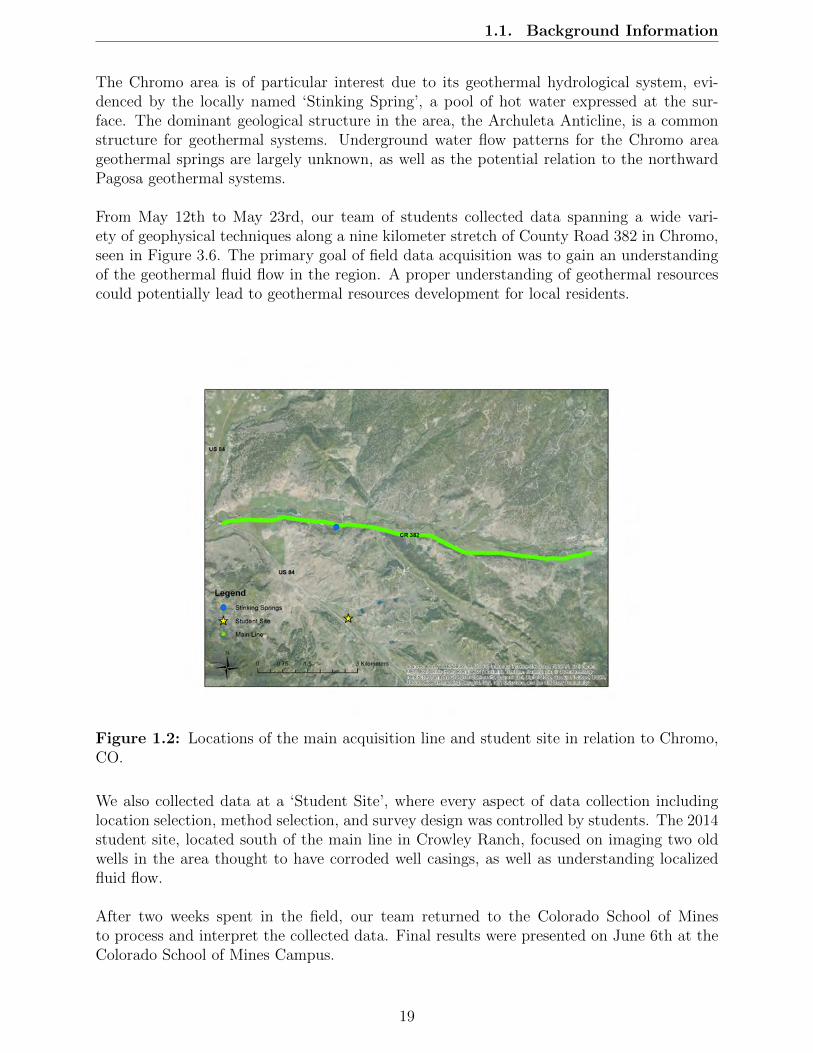
The Chromo area is of particular interest due to its geothermal hydrological system, evi-denced by the locally named ‘Stinking Spring’, a pool of hot water expressed at the sur-face. The dominant geological structure in the area, the Archuleta Anticline, is a commonstructure for geothermal systems. Underground water flow patterns for the Chromo areageothermal springs are largely unknown, as well as the potential relation to the northwardPagosa geothermal systems.
From May 12th to May 23rd, our team of students collected data spanning a wide vari-ety of geophysical techniques along a nine kilometer stretch of County Road 382 in Chromo,seen in Figure 3.6. The primary goal of field data acquisition was to gain an understandingof the geothermal fluid flow in the region. A proper understanding of geothermal resourcescould potentially lead to geothermal resources development for local residents.
Figure 1.2: Locations of the main acquisition line and student site in relation to Chromo,CO.
We also collected data at a ‘Student Site’, where every aspect of data collection includinglocation selection, method selection, and survey design was controlled by students. The 2014student site, located south of the main line in Crowley Ranch, focused on imaging two oldwells in the area thought to have corroded well casings, as well as understanding localizedfluid flow.
After two weeks spent in the field, our team returned to the Colorado School of Minesto process and interpret the collected data. Final results were presented on June 6th at theColorado School of Mines Campus.
19

1.2. Objectives
1.2 Objectives
The fundamental goal of this field camp and related geothermal investigation was to pro-vide an applied field geophysics experience for our student team. The two weeks spent inthe field helped to transition classroom concepts and theory into practical data acquisitionskills. Field safety and risk assessment were prioritized during all field activities. The finaltwo weeks focused on strengthening critical thinking and analytic skills through data reduc-tion and processing on the data collected in the field. Working with a data set collected firsthand emphasizes the many challenges that need to be overcome for raw data. Combiningboth distinct sections together creates a cohesive field session that augments in-class educa-tion. Understanding the entire geophysics workflow from survey design to data acquisitionand data processing is a critical skill for geophysicists to learn, and one that is reinforcedthroughout field camp.
While education was the foremost priority, the scientific content contained in this reportrepresents a real geophysical investigation with results pertinent to the host communities.The town of Chromo, situated 25 miles south of Pagosa Springs, also has geothermal wa-ter springs present in the area. While Chromo is significantly less populated then PagosaSprings, the anticlinal geologic structure is a common geothermal setting, suggesting that thetown’s residents and ranchers could utilize the resource if characterized properly. Our teamof students approached this year’s field camp with the overarching goal of understanding thegeothermal fluid flow in the region. The main line of data collection stretched clear acrossthe Stinking Springs, the largest surface evidence for the geothermal system. We performednumerous geophysical survey methods in order to gain as much information possible aboutthe potential energy resource flowing underneath Chromo.
20

CHAPTER 2
GEOLOGY
2.1 Geologic History
Chromo is located in the southern part of Colorado, 25 miles south of Pagosa Springs.Geologically, Chromo is part of the Archuleta anticlinorium. The anticlinorium is a complexbelt consisting of numerous faults and folds that come together to create the northeasternflank of the San Juan basin. The primary geologic feature specific to the Chromo area is theChromo anticline which ranges from the southeastern part of Archuleta County, Colorado tothe northern part of Rio Arriba County in New Mexico. The Chromo anticline is comprisedof several different rock layers that range in age from the Precambrian basement to the LewisShale of the Upper Cretaceous period.
2.1.1 Subsurface Geology
Sediments around the San Juan basin are deposited on the Precambrian basement. Thebasement is made up of both metamorphic and igneous crystalline rocks consisting of ap-proximately 45 percent granitic rocks, 30 percent schist and gneiss, 15 percent quartzite andphyllite and 10 percent greenstone [22]. No outcrops of the basement can be seen in thearea, but from previous research done on this area, we can assume that over time there hasbeen a major uplift of the basement [35]. Thicknesses and lithologic descriptions can be seenin Figure 2.1.
Above the basement rock lays the Entrada Sandstone which was formed in the late Jurassicperiod. Formation occurred by wind and alluvial deposits laid by the flanks of the basementrock. Near the crest of the anticline, it is estimated that the Entrada Sandstone is approx-imately 60 meters (200 feet) thick. Within this sandstone, the sand grains are generallysub-rounded, fine to coarse, and has a light gray color [13].
Overlying the Entrada sandstone is the Todilto limestone. This layer consists of embed-ded, dark gray gypsum and limestones which were likely deposited in lagoon conditions.The Todilto limestone has a consistent thickness throughout the Chromo anticline of ap-proximately 30 meters (100 feet).
The last formation, deposited in the Jurassic period, is the Morrison formation. The Morrisonformation overlies the Todilito and Entrada limestones and is made up of shales, sandstonesand limestone of fluvial or flood plain origins [13]. Colors range from gray, green and red
21

2.1. Geologic History
shales and white sandstone. It is hard to say exactly where the time boundary between theJurassic and Cretaceous deposits is, so the upper part of the Morrison formation could likelybe in the early Cretaceous period.
Dakota Sandstone overlies the Morrison formation, and is the first rock type that appearsfully in the Upper Cretaceous period ranging from 55-85 meters (177-270 feet) thick. Thismember is considered to be a transgressive sandstone, and as time progress, the layer wascovered by dark shales and limestones [13]. The Dakota Sandstone is further broken upinto three layers. The lower member is a cross-bedded conglomerate that with a medium tocoarse grain size. Above this layer is a darker gray, carbonaceous silty shale, followed by athird buff layer of fine grained sandstone.
Figure 2.1: Strategraphic Section of the Chromo Area [13].
22

2.1. Geologic History
2.1.2 Surface Geology
Directly above the Dakota Sandstone is about 1900 feet of dark gray marine shale whichmakes up the Mancos Shale unit. At the location of the main line over the Chromo anticlinethe Mancos shale is approximately 2100 feet thick, but only the top 1500 feet of this sectionis exposed at the surface of the anticline. This layer contains units consistent to the Bentonshale (Graneros shale, Greenhorn limestone, Carlile shale, and Niobrara shale). There areno clear exposures with the exception of some drainages and road cuts. On the surface, theMancos shale can be subdivided into two layers based on the lithology. The Juana Lopez-Niobrara and the upper shale member are divided. Changes can be seen by looking at thecolor change of the soil and a change in vegetation.
The Mesa Verde formation is directly above the Mancos shale and has a conformable andgradational contact, meaning that the sandy shales of the Mancos move upward into thesandstone of the Mesaverde formation. The Mesa Verde formation can be seen in outcropsalong the flanks of the Chromo anticline parallel to the Mancos shale. Colors range frombuff to gray and can be seen as sandstone ledges. The thickness of this member is estimatedto range from 250-365 feet and consists of both sandstone and shale.
Lewis shale is the final layer of the Upper Cretaceous period and is also the last mem-ber where surface units can be found. Much like the Mancos shale, the Lewis shale outcropscan be found along the flanks of the anticline and are also very similar in appearance. Thebest way to differentiate these two types of shale is to find the presence of concretionaryzones, look for faunal evidence and the stratigraphic position [13]. Lewis shale ranges fromdark gray to black shale in color which often weathers to be a light gray.
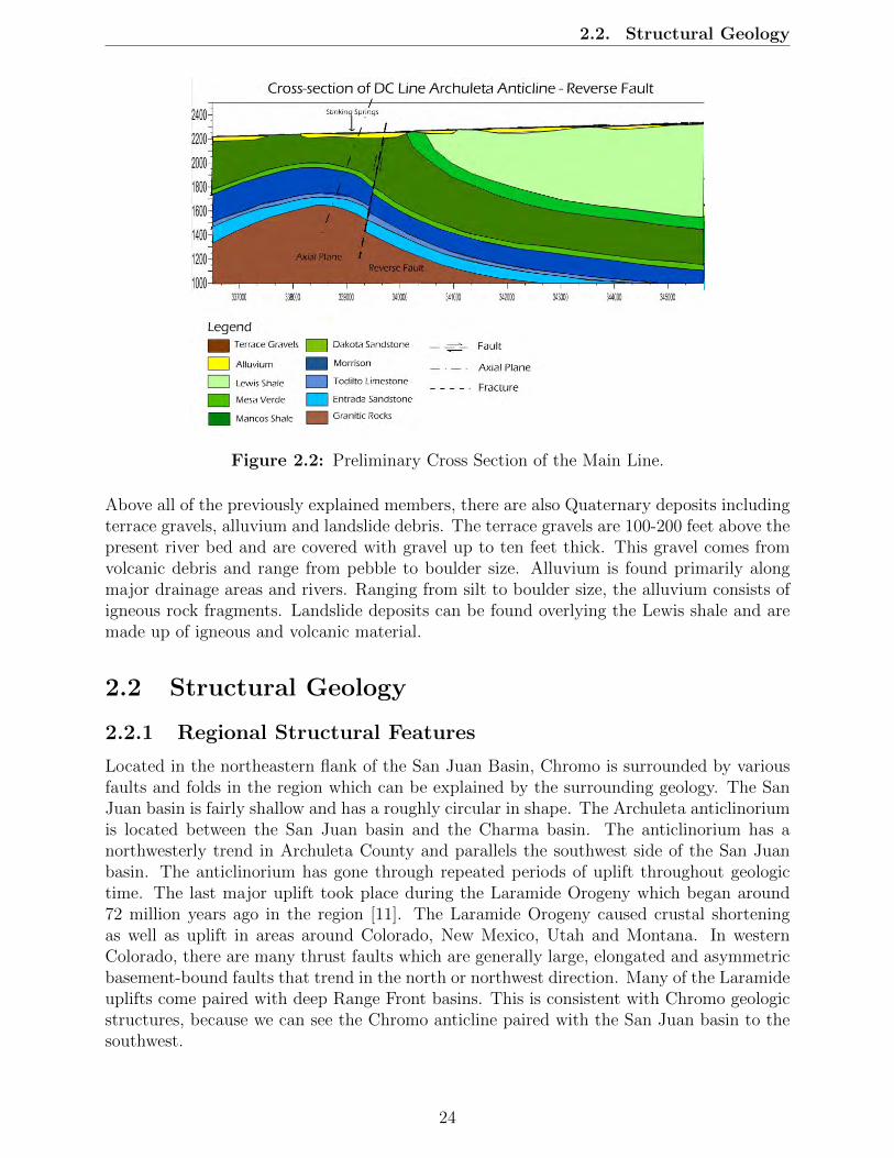
After learning more about the different rock types through research and observing surfacegeology in the field, we were able to create a preliminary cross section of the area and canbe seen in Figure 2.2.
23
2.2. Structural Geology
Figure 2.2: Preliminary Cross Section of the Main Line.
Above all of the previously explained members, there are also Quaternary deposits includingterrace gravels, alluvium and landslide debris. The terrace gravels are 100-200 feet above thepresent river bed and are covered with gravel up to ten feet thick. This gravel comes fromvolcanic debris and range from pebble to boulder size. Alluvium is found primarily alongmajor drainage areas and rivers. Ranging from silt to boulder size, the alluvium consists ofigneous rock fragments. Landslide deposits can be found overlying the Lewis shale and aremade up of igneous and volcanic material.
2.2 Structural Geology
2.2.1 Regional Structural Features
Located in the northeastern flank of the San Juan Basin, Chromo is surrounded by variousfaults and folds in the region which can be explained by the surrounding geology. The SanJuan basin is fairly shallow and has a roughly circular in shape. The Archuleta anticlinoriumis located between the San Juan basin and the Charma basin. The anticlinorium has anorthwesterly trend in Archuleta County and parallels the southwest side of the San Juanbasin. The anticlinorium has gone through repeated periods of uplift throughout geologictime. The last major uplift took place during the Laramide Orogeny which began around72 million years ago in the region [11]. The Laramide Orogeny caused crustal shorteningas well as uplift in areas around Colorado, New Mexico, Utah and Montana. In westernColorado, there are many thrust faults which are generally large, elongated and asymmetricbasement-bound faults that trend in the north or northwest direction. Many of the Laramideuplifts come paired with deep Range Front basins. This is consistent with Chromo geologicstructures, because we can see the Chromo anticline paired with the San Juan basin to thesouthwest.
24

2.2. Structural Geology
Figure 2.3: Geologic Map of Archuleta County.
Primary structural features can be seen in Figure 2.3, noting that the red line representsthe main survey line in Chromo. Narrow belts of folding show the persisting uplift whichdivides the two basins. The faults and folds tend to follow this trend, but there are alsomany transverse structures in the area. Paralleling the Archuleta anticlinorium to the east,the Chama basin is found. The Chama basin has a relief of about 3000 feet while the SanJuan basin has about 9000 feet of relief. This difference in relief suggests that Chama basinwas depressed less than the San Juan basin. To the east, the San Juan Mountains are theboundary to the Chama basin and the northeastern boundary to the Archuleta anticlinorium.The San Juan Mountains are made up of Tertiary volcanics on the surface and overlay theolder igneous and sedimentary rocks.
2.2.2 Local Structural Features
Regional geology is important to understand the big picture of an area. But for the purposeof the surveys we conducted, the local structural features, such as the Chromo anticline,are of greater importance. The Chromo anticline is the most prominent feature within theArchuleta anticlinorium and has a northwest trend. The anticline takes on an asymmetricalshape with dips around 35 degrees to the northeast and 5 degrees to the southwest flankof the anticline. Most sedimentary formations hold a constant thickness throughout thestructure which would suggest that the folding of the Chromo anticline was due to flexurefolding [13]. When flexural slip occurs, the slip occurs on the bedding planes rather thanthe hinge. There is no slip at the hinge. Without the use of subsurface images, it is hardto map the crest of the anticline due to the lack of exposures of the Mancos shale. Due tolack of previous geophysical investigation, the crest of the anticline has not previously beenmapped. To the north of the Chromo anticline, is the Coyote Park syncline that can be seenin Figure 2.4. The syncline axis has a east- west trend and plunges to the west. Like theanticline, the syncline is asymmetrical and has dips around 10 degrees to 30 degrees on theflank. Chama basin is to the northeast of the synclinal axis with the axis located about 2.5miles away from the Chromo anticline axis. The basin is nearly flat and plunges less than 1degree. The geology of the Chromo anticline can be seen in Figure 2.4.
25

2.2. Structural Geology
Figure 2.4: Geologic Map of the Chromo Anticline.
26

2.3. Field Observations
Faults in the mapped area in Figure 2.4 are generally very small. The smallest faults on themap show displacements of only 50 feet where the larger faults show displacements of up to250 feet. The one potential exception to these values is a fault to the western edge of themap that shows displacement of around 800 feet. This fault is significantly to the west ofthe main line, so this will not be seen in any of the geophysical data collected along the mainline. The other, smaller faults appear in the northern section of the map and, as stated byConley, all faults are normal faults. Beyond the Mesa Verde outcrops, the faults are hard totrace due to deep soil cover and poor exposures.
2.3 Field Observations
In an attempt to orient ourselves with the area, one day prior to the collection of geophysicaldata was spent examining the local geology. Stops made in the tour of Chromo geology can beseen in Figure 2.5. Exploring the geology of the Chromo area allowed us to locate structuralfeatures, stratigraphic units and wells in the area which was used in an attempt to make apreliminary cross section of the area. This cross section can be seen in Figure 2.2. As varioussubsurface images from geophysical methods became available, the cross section changed inorder to reflect the other data sets. During the geology tour of Chromo, two wells, drilled inthe 1930s, were seen. Flowing Well was of particular interest and became the Student Sitewhich was situated on the Mancos Shale. The base site for this survey was at the Chromofire station which was also situated on the Mancos Shale just on the edge of the Mesa Verdeformation.
Figure 2.5: Map of Geology Scouting Locations
27
2.4. Geothermal Source
2.4 Geothermal Source
In a water-dominated geothermal system, ground water circulates at a depth and ascendsfrom buoyancy in reservoirs with a uniform temperature [31]. Water dominated systems canbe seen on the surface as hot springs, geysers and travertine deposits. For a hot spring tobe produced, there are five geologic features that must occur. The most important factor isthat there must be some source of heat. This heat source can come from Earth’s geothermalgradient or from localized volcanism [35].
There must also be a reservoir or aquifer within the system to allow for the accumulation ofgeothermal water. Previous work done in the Pagosa Springs area suggests that the primaryaquifer is in the Dakota sandstone because the water temperatures are greater here than inthe surrounding rock layers [13]. The existence of an aquifer is dependent on the presenceof a recharge mechanism. Recharge in the Chromo area comes from snow melt, which thendrains into the rivers. The last two components of a geothermal system consist of a caprock and migration route. The cap rock lies on the top of the aquifer and is impermeable.This keeps the water from escaping from the system. Due to its low permeability and strati-graphic position, it is suggested that the Mancos shale is the cap rock. The migration routeincludes percolation from rain and snow melt into the ground as well as a path back to thesurface to create a hot spring. The path back to the surface often occurs in either fractures,fault planes, or both, so these structures were investigated further in the area in order tointegrate geophysical methods with the local geology of Chromo.
2.5 Hydrology
The direction of subsurface flow cannot be seen by simply looking at the flow direction ofrivers and streams in the surrounding area, yet looking at these features can help to explorepossibilities of subsurface flow. Near Pagosa Springs is the San Juan River. The riverflows from east to west and is fed by various tributary rivers flowing toward the southwest.Regional fluid flow direction is determined by the topography of the San Juan Mountains.Before reaching Navajo Lake in New Mexico, the San Juan River meets the Navajo River,which flows to the west, directly through Chromo and can be seen from the main surveyline. There is a relative abundance of surface water here which leaves a poor water qualityin shallow aquifers. Due to these limitations, there is groundwater development here [15].Primary aquifers in the area are found in the Mancos shale and Dakota sandstone layers,though a fraction of wells have been drilled in the Morrison formation, also. The flowof groundwater in the Mancos shale layer results from both fracture and porosity. Anygroundwater found in the Dakota sandstone comes from fracture porosity and is confined.Subsurface flow in the area was imaged using the self-potential (SP) method and can be seenin the interpretations sections of this report.
28

CHAPTER 3
GEOPHYSICS
In order to understand the geophysical data and interpretations containted in this report, itis important to understand the background and theory behind each individual method. Thissection will introduce some basic geophysical concepts as well detail the background detailsfor each geophysical method for which we aquired data in Chromo. Additional theory anddetailed processing information can be found in the appendices.
3.1 Active vs. Passive Source
Geophysical methodology is often refered to as being active or passive source. While bothtypes of methods record the response of physical properties of subsurface rock units, activesource generate and record resposnes using additional energy controlled by the surface crewteam. For example, the seismic aquisition in this experiment was an active source method,using Vibroseis trucks to actively shake the earth and create acoustic energy which reflectsoff layers and is recorded back at the surface. Passive source methods measure the responseof the subsurface without any disturbance. Gravity and magnetics are classic passive sourcemethods, purely recording the responses from the earth’s natural fields.
3.2 Depth of Investigation
The depth in the earth to which geophysical techniques can record data with a strong signalto noise ratio varies greatly by method. Because different types of energy used in activesource experiements attenuate into the earth at varying rates, certain methods are moreuseful for imaging deep, and others shallow. As a general rule of thumb, lower frequencyenergy allows for deeper imaging, although the resolution is decreased. Higher frequencyenergy attuates quickly and images only shallow features, but with increasied resolution.
3.3 Modeling Techniques
Geophysical data processing involves creating models from data collected in the field. Inorder to understand the terminology used in individual sections, it is first important tounderstand the core concepts of basic modeling techniques. Figure 3.1 provides a simplevisual explanation of the modeling process.
29

3.3. Modeling Techniques
3.3.1 Forward Modeling
Forward modeling is the process of simulating the response of a particular method usingestimates of subsurface structure and geologic units. Forward modeling code takes an inputof a subsurface model file and produces a simulated data file as an output. Forward modelingis useful for understanding in a general sense what data should look like before it is collected.For example, since our study area contains a known anticline structure, forward models couldbe used to simulate how the anticline appears in each data-set. Forward models are alsooften used to help design survey parameters that properly image the desired structures.
3.3.2 Inverse Modeling
Inverse modeling is the process of reconstructing subsurface structure from collected data.Inverse modeling code uses field data as an input and outputs a subsurface model thatcould have produced the collected data. However, inverse modeling does not output geologicinformation, rather a distribution of physical properties based on the particular methodbeing used. For example, a gravity inversion process takes a corrected gravity field data fileas an input and outputs a distribution of density in the subsurface that fits the data. Often,inversion results are non-unique, allowing multiple different models to fit the data. In thesecases, additional information is used to help constrain the inversion process and narrow thenumber of models that can fit the field data. Inverse models are often combined with priorgeologic knowledge and geologic assumptions to help interpret the rock layers in the surveyarea.
Figure 3.1: Visual flowchart detailing the interaction between data & models throughinverse and forward modeling.
30

3.4. Survey
3.4 Survey
3.4.1 Introduction
Surveying is a crucial component of data acquisition and processing for all geophysical meth-ods. Surveying is used to determine the location of markers within a geophysical survey inorder to accurately create models that show the true location of variations within the sub-surface. The surveying methods used for the characterization of the Chromo region werehandheld GPS and differential GPS. All points were plotted using the WGS 1984 UTM Zone13N coordinate system.
3.4.2 Background/Theory
GPS uses the known location of satellites orbiting Earth to determine positions of latitude,longitude, and elevation on Earth. GPS involves a constellation of 24 satellites divided intosix orbital planes, each containing four satellites. Each satellite has an elliptical orbit aroundthe Earth with a semi-major axis of 26,578 km and a period of approximately twelve hours.All satellites are monitored by five base stations located around the Earth, with the mainstation located in Colorado Springs, Colorado. These base stations transmit clock updatesand positioning to satellites ([45]). A GPS receiver needs to receive signals from at leastfour satellites in order to determine the receiver’s location. The signals produced from GPSsatellites are low power radio signals, which travel by line of sight, meaning they will typicallynot travel through solid objects. Signals contain information about the satellite ID, currentsatellite conditions, and satellite location and orbital information. If more satellite signalsare available to the receiver, the accuracy of the position increases. The GPS receiver isable determine its position by taking the known satellite positions and using triangulation,which is done by calculating the time difference between the transmitted and received signalsfrom all satellites ([30]). Availability of satellite signal depends on the time of day as well aspossible signal barriers such as buildings, foliage, or mountains.
3.4.3 Differential GPS
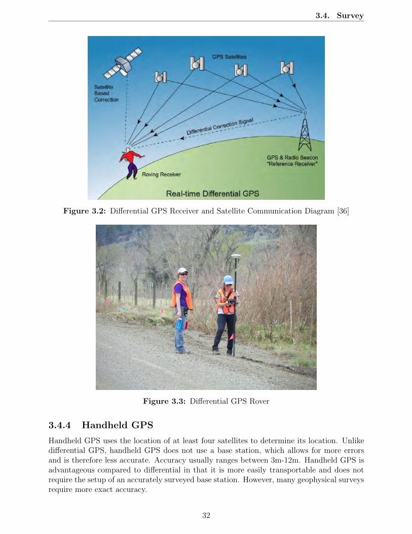
Differential GPS uses the cooperation of two receivers to acquire precise positioning infor-mation within one meter. One station, the base, is placed at a point that has been veryaccurately surveyed and stays stationary during the survey. The other station, the rover,acquires GPS data for all desired points on the survey. Both receivers obtain available satel-lite signals (at least four, which have some error associated with them depending on whathappened to the signal on the way down). Because distances between points on Earth arerelatively small compared to the distance from Earth to the satellite, we can assume thesignal to the base and rover will have essentially the same timing errors. This allows thebase station to use its known position to calculate what the GPS timing signals should becompared to what they actually are. This difference is referred to as the error correctionfactor. The base station can then transmit the error information to the rover for locationmeasurement corrections. To ensure accurate timing corrections, the base station calculateserror for all visible satellites even though the rover may not use all of them ([28]). DifferentialGPS provides the advantage of more accurate survey measurements compared to handheldGPS.
31
3.4. Survey
Figure 3.2: Differential GPS Receiver and Satellite Communication Diagram [36]
Figure 3.3: Differential GPS Rover
3.4.4 Handheld GPS
Handheld GPS uses the location of at least four satellites to determine its location. Unlikedifferential GPS, handheld GPS does not use a base station, which allows for more errorsand is therefore less accurate. Accuracy usually ranges between 3m-12m. Handheld GPS isadvantageous compared to differential in that it is more easily transportable and does notrequire the setup of an accurately surveyed base station. However, many geophysical surveysrequire more exact accuracy.
32

3.4. Survey
Figure 3.4: Handheld GPS [7]
3.4.5 GPS used with Geophysical Methods
Differential GPS and handheld GPS offer different advantages and disadvantages. Somegeophysical methods do not require extreme accuracy while other methods require locationaccuracy on the order of centimeters. Most of the methods used on the surveys in Chromowere located using differential GPS due to few time restraints for the surveying crew. Deepseismic, hammer seismic, DC resistivity, self-potential, magnetics, ground penetrating radarand gravity surveys were all located using differential GPS. Ground penetrating radar (on thestudent site) and electromagnetic surveys were located using handheld GPS. Magnetotelluricssurveys were located using an internal GPS system within the instrument.
Figure 3.5: GPS type for different geophysical methods
33

3.4. Survey
3.4.6 ArcMap
ArcMap is a component within the program ArcGIS that is used to display geospatial data.ArcMap has several built in maps, such as satellite and topographic maps, with accuratelocation information. To display surveys and points of interest, we imported Excel documentscontaining the UTM coordinates of all of the surveys into ArcMap, which the program thenplotted in the correct positions. We used ArcMap to display the locations of the varioussurveys on the main line and within the student survey grid. Additionally, we included thelocations of various points of interest, such as geologic outcrops, to help processing teamsorient where the surveys took place relative to the regional geology.
3.4.7 Survey Locations
Our geophysical surveys in Chromo consisted of the Main Line and the Student site, asseen below in Figure 3.6. The Main Line spanned a 9 km section of county highway 382,running E-W. The Student Site location was south of the Main Line, located in CrowleyRanch centered around a feature referred to as the Flowing Well. This site consisted of a100 m by 200 m grid around the Flowing Well.
Figure 3.6: Location of the Main Line and Student site with respect to the Chromo area.
34

3.5. Gravity
3.5 Gravity
3.5.1 Introduction
Gravity is a passive geophysical method that uses the earth’s gravitational field to detectdensity variations within the subsurface. A gravimeter is used to measure the gravitationalacceleration at discrete points along the survey. Differences in acceleration measurementsare indicative of density variations which can tell us information about the structure of thesubsurface, including the presence of faults and folds. On our main line in Chromo, thegeologic layer that will give the greatest density contrast is the Precambrian basement. Ourgoal is to integrate gravity with other methods in order to map the Archuleta Arch andlocate potential faults along the main line which could act as conduits for geothermal fluidflow.
3.5.2 Background/Theory
The gravity method is based on Newton’s Universal Gravitational Law and Newton’s SecondLaw of Motion, seen in Equations 3.4 and 3.5, respectively. In Newton’s Universal Gravita-tional Law, G represents the gravitational constant and F is the gravitational force betweentwo bodies, m1 and m2, which are separated by a distance r. In Newton’s Second Law ofMotion, F represents a force produced by a mass, m, with an acceleration, a. By combiningthese two laws, we can determine an equation that may be used to calculate the earth’sgravitational field given in Equation 3.6, where g is the gravitational acceleration, M is themass of the earth, and r is the distance from the center of the earth to the point of interest onEarth’s surface. Units of acceleration are most commonly seen in m/s2. However, in gravitysurveys, we use units of Gals and milliGals (mGal). One mGal is equal to 1× 10⁻⁵m/s2. Toprovide some perspective, an apple would produce a gravitational response of approximately5 mGal and the earths response is approximately 9.8× 10⁵ mGal.
F = Gm1m2
r2(3.1)
35

3.5. Gravity
where G is the gravitational constant and r is the distance to the center of the earth.
F = ma (3.2)
Combining both laws, we can solve for gravitational acceleration in Equation 3.6 (where Mis the mass of the earth).
g =GM
r2(3.3)
All of the data collected on the main line was obtained by the Scintrex Autograv CG-5,which is a relative gravimeter (see appendix for operating procedure). The CG-5 and otherrelative gravimeters calculate gravitational acceleration by measuring the displacement of aspring within the device which shifts based on the gravitational acceleration, and thereforethe mass beneath it. For each point, the CG-5 records the gravitational acceleration multipletimes and stacks each measurement based on input parameters. The CG-5 measurementsare precise within 5 µGal. Due to this high sensitivity, it is important to take note of whenlarge objects are near the gravimeter, which may cause false anomalies. Additionally, datacollected in the field needs to be corrected for time, elevation, terrain, geometry, and lati-tude, all of which affect gravity measurements and can also produce false anomalies if thedata is not corrected appropriately. Once all corrections are applied, true density contrastsand anomalies can be seen in the data.
The depth of investigation for gravity surveys is dependent on the location of the great-est density contrast. This means that strong contrasts located at deeper depths result in agreater depth of investigation, whereas shallow contrast depths result in shallower depthsof investigation. In Chromo, the greatest density contrast occurs between the Precambrianbasement and the younger layers that are shale and sandstone. This depth varied throughoutthe survey due to the shape of the anticline in addition to other geologic features. It is alsoimportant take into account the length of the survey line. The length of the survey does notaffect the depth of investigation; however, it does affect the understanding of the large scalegeologic trends.
36

3.6. Magnetics
3.6 Magnetics
3.6.1 Introduction
The Earth has a natural magnetic field that interacts differently with the surface and sub-surface materials depending on the location on the Earth. The strength of the magnetic fieldand angle at which the field penetrates the Earth changes with location (Figure 3.9). Mag-netics surveying is a passive geophysical method used to measure the magnetic field createdby subsurface anomalies by removing the natural, external magnetic field of the Earth.
Figure 3.9: Sketch of the Earth’s primary magnetic field. [37]
Magnetics surveys help to identify underground features that are able to be magnetized.Magnetic surveys are passive, simply meaning magnetics measure the natural magnetic fieldinstead of inducing a secondary field. Using the data gathered by magnetics, physical prop-erties such as magnetic susceptibility can be extracted, and the subsurface can subsequentlybe identified.
37
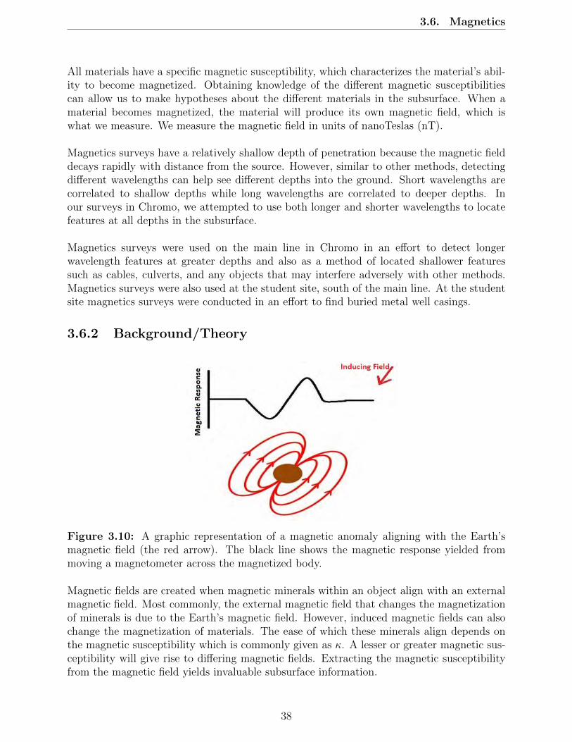
3.6. Magnetics
All materials have a specific magnetic susceptibility, which characterizes the material’s abil-ity to become magnetized. Obtaining knowledge of the different magnetic susceptibilitiescan allow us to make hypotheses about the different materials in the subsurface. When amaterial becomes magnetized, the material will produce its own magnetic field, which iswhat we measure. We measure the magnetic field in units of nanoTeslas (nT).
Magnetics surveys have a relatively shallow depth of penetration because the magnetic fielddecays rapidly with distance from the source. However, similar to other methods, detectingdifferent wavelengths can help see different depths into the ground. Short wavelengths arecorrelated to shallow depths while long wavelengths are correlated to deeper depths. Inour surveys in Chromo, we attempted to use both longer and shorter wavelengths to locatefeatures at all depths in the subsurface.
Magnetics surveys were used on the main line in Chromo in an effort to detect longerwavelength features at greater depths and also as a method of located shallower featuressuch as cables, culverts, and any objects that may interfere adversely with other methods.Magnetics surveys were also used at the student site, south of the main line. At the studentsite magnetics surveys were conducted in an effort to find buried metal well casings.
3.6.2 Background/Theory
Figure 3.10: A graphic representation of a magnetic anomaly aligning with the Earth’smagnetic field (the red arrow). The black line shows the magnetic response yielded frommoving a magnetometer across the magnetized body.
Magnetic fields are created when magnetic minerals within an object align with an externalmagnetic field. Most commonly, the external magnetic field that changes the magnetizationof minerals is due to the Earth’s magnetic field. However, induced magnetic fields can alsochange the magnetization of materials. The ease of which these minerals align depends onthe magnetic susceptibility which is commonly given as κ. A lesser or greater magnetic sus-ceptibility will give rise to differing magnetic fields. Extracting the magnetic susceptibilityfrom the magnetic field yields invaluable subsurface information.
38

3.6. Magnetics
The basic source of all magnetic fields is moving charges. In short, moving charges in-duce an electrical field. The variations within an electrical field create a magnetic field. Thisis demonstrated by the following equation which states the curl of an electrical field is equalto the negative partial derivative of the magnetic field with respect to time:
∇× E =∂B
∂t(3.4)
Where E is the electrical field, and B is the magnetic field.
This equation physically means that as the electrical field changes in space (i.e. the chargesare moving), the magnetic field is changing in time. If charges are moving, then a magneticfield will be induced.
Magnetic fields themselves are not divergent. There is no net flux loss or gain over a closesurface. For whatever amount of flux enters the surface enclosing a magnetic field there isan equal amount of flux leaving the surface. In simpler terms, whatever enters the systemis equal to what leaves the system.
∮
ds
B · n ds = 0 (3.5)
Where B is the magnetic field, n is the normal vector, and ds is the surface of integration.
As previously stated, magnetic susceptibility controls how easily an object is magnetized.The magnetic susceptibility of an object also controls the magnetic permeability of an object,which can then be related to the magnetization of an object.
µ = µ(1 + κ) (3.6)
Where µ is the magnetic permeability of an object, µ is the magnetic permeability in avacuum, and κ is magnetic susceptibility.
−→M =
κ−→B
µ(3.7)
Where−→M is the magnetization, κ is the magnetic susceptibility,
−→B is the magnetic field,
and µ is the magnetic permeability.
As Equation 3.7 shows, magnetization contains several of the properties necessary for thedistinction of layers and rock types.
For this survey we utilized two cesium vapor magnetometers and one proton precessionmagnetometer. Proton precession magnetometers work by injecting a current in the solenoidcreating a strong magnetic field around the internal fluid. The protons then align with thisfield until the current is interrupted [44]. The protons proceed to align with the externalfield creating a weak internal magnetic field. This magnetic field is then digitalized andrecorded. The proton precession magnetometer is commonly used to measure the changesthat the Earth’s magnetic field incurs over time.
39

3.6. Magnetics
The cesium vapor magnetometers operate under the understanding that a cesium atomcan exist in any of nine energy levels. When a cesium atom is excited to the point of in-creasing in energy level, the cesium atom will drop a photon and jump into the next energystate [44]. Theoretically, at some point all cesium atoms will drop through and be measured.For most surveys, a small alternating current is used to induce a magnetic field within themagnetometer. Variations in the external magnetic field will influence the internal magneticfield and cause the protons to react. The resulting changes in photons are then measured.
We used both the proton precession and cesium magnetometer for the investigation of theChromo area. The proton precession magnetometer typically is used as a base station as thereadings of the background field can be taken. This is important as the Earth’s magneticfield is variable, changing throughout the day. The readings from the cesium magnetome-ter, which is used to take measurements at different locations, will show the effects of thechanging background field. The variability in the Earth’s magnetic field is then correctedfor by the data taken by the proton precession magnetometer which has observed the de-viations. Theoretically, removing the background field from the data taken by the cesiummagnetometer will result in just the anomalous field being present. The anomalous field isthen used in identifying components of the subsurface.
40

3.7. Self-Potential
3.7 Self-Potential
3.7.1 Introduction
Self-potential is a passive geophysical method in which both reference and roving non-polarized electrodes are used to measure voltage across the electric field produced by naturaltelluric currents in the subsurface. These natural currents are a result of the flow of watercarrying excess charge, as well as the corrosion of metallic bodies underground.
The distribution of lateral changes in the voltage, or streaming potential, across stationscan shed light upon fluid flow in the subsurface. The shape of the potential gives an idea ofthe amount and direction of fluid flow. However, without an idea of subsurface resistivitydistribution, it is difficult to accurately determine volume or the geometry of the flow, hencewhy self-potential was combined with DC resistivity at the Flowing Well site. This difficultywill be discussed further in the background section of the self-potential method.
Fluid flow is an important aspect of characterizing the geothermal system of the Chromoarea. Finding areas of high fluid outflow may help uncover the conduit by which the wateris travelling up to the surface to form the hot springs present in the area. Self-potentialcan also help uncover the location of metallic bodies in the subsurface, like the corrodedwell casings present at the Student Site. Uncovering these casings could be beneficial to thelandowners; knowing the precise locations of the wells allows landowners to have the optionto properly reseal the wells in order to prevent further leakage of hydrocarbons.
Self-potential signals are associated with electrical currents flowing in the ground. There areseveral sources for self-potential signals: geobattery systems associated with ore body cor-rosion, the streaming current from the drag of excess charge present in the pore water, andthe diffusion current resulting from gradients in the chemical potentials of charge carriers.[40].
3.7.2 Background/Theory
The two main sources of the current density in the self-potential method are the streamingcurrent resulting from the advective transport of pore water containing electrical charges,and diffusion currents from the gradients of concentration of ionic species in the pore water.In both of these cases, there is a porous material saturated with brine, and the electricalcurrent density, j, can be expressed as follows in a generalized form of Ohms Law:
j = σ0E + js (3.8)
where E is the electrical field (V/m), js is a source current density, and σ is the DC electricalconductivity of the material, to be discussed in detail in the following DC resistivity section.Since total current density, j is conservative, meaning that all current entering a controlledvolume must also exit that volume, the following continuity equation can be obtained:
∇ · j = 0 (3.9)
Electric fields can be written as a function of electric potentia, ψl:
41

3.7. Self-Potential
E = −∇ψ (3.10)
The self-potential field is a solution to the Poisson Equation, the fundamental field equa-tion in the interpretation of SP signals This equation is obtained from combining both Ohmslaw, a constitutive equation, (3.8) and the continuity equation (3.9) for current density:
∇ · σ0∇ψ = ∇ · js = J (3.11)
where J represents a volumetric charge source or sink term, sigma0 represents conductivity,and ψ represents potential.
Equation 3.11 states that the distribution of electric potential is created by a volumetricsource or sink term, namely the divergence of the source current density, which dependson the flow and the chemistry of the pore water contained within a formation as well asthe distribution of electrical conductivity. The presence of a source current density is onlypossible with a system that is in a steady state of thermodynamic disequilibrium; the sourcecurrent density is associated with any disturbance that could potentially affect the transportof charge-carriers throughout the subsurface.
Measuring the potential allows us to solve for the charge source or sink term. Then thedistribution of electrical conductivity, or the geometry can also be determined However, thisis a non-linear inversion problem, equivalent to that found in DC resistivity tomography (tobe discussed in the following section), except that in the self-potential method, unlike DC,internal currents are used in place of imposed currents. Instead, a better approach is toassume that the distribution of electrical conductivity is known, and to then compute eitherthe volumetric charge source or sink term, or the source current density. This inversionproblem is linear, but still underdetermined, meaning that there are many possible solutionsto the given problem and the amount of data is far less than the amount of unknowns. How-ever, combining conductivity data from DC resistivity acquisition with self-potential datawould result in a more accurate, constrained SP inversion model. This model could be usedto map fluid flow in the subsurface, as well as point towards the locations of corroded wellcasings underground at the Flowing Well site. Inversion will be discussed in more detail inthe processing portion of self-potential and direct current resistivity methods [39].
Additional theory for the self-potential method can be found in the Appendix.
42
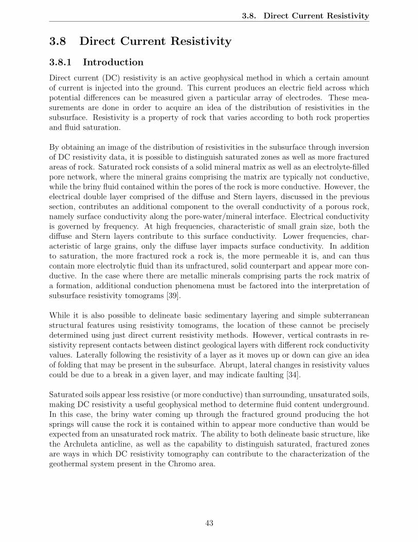
3.8. Direct Current Resistivity
3.8 Direct Current Resistivity
3.8.1 Introduction
Direct current (DC) resistivity is an active geophysical method in which a certain amountof current is injected into the ground. This current produces an electric field across whichpotential differences can be measured given a particular array of electrodes. These mea-surements are done in order to acquire an idea of the distribution of resistivities in thesubsurface. Resistivity is a property of rock that varies according to both rock propertiesand fluid saturation.
By obtaining an image of the distribution of resistivities in the subsurface through inversionof DC resistivity data, it is possible to distinguish saturated zones as well as more fracturedareas of rock. Saturated rock consists of a solid mineral matrix as well as an electrolyte-filledpore network, where the mineral grains comprising the matrix are typically not conductive,while the briny fluid contained within the pores of the rock is more conductive. However, theelectrical double layer comprised of the diffuse and Stern layers, discussed in the previoussection, contributes an additional component to the overall conductivity of a porous rock,namely surface conductivity along the pore-water/mineral interface. Electrical conductivityis governed by frequency. At high frequencies, characteristic of small grain size, both thediffuse and Stern layers contribute to this surface conductivity. Lower frequencies, char-acteristic of large grains, only the diffuse layer impacts surface conductivity. In additionto saturation, the more fractured rock a rock is, the more permeable it is, and can thuscontain more electrolytic fluid than its unfractured, solid counterpart and appear more con-ductive. In the case where there are metallic minerals comprising parts the rock matrix ofa formation, additional conduction phenomena must be factored into the interpretation ofsubsurface resistivity tomograms [39].
While it is also possible to delineate basic sedimentary layering and simple subterraneanstructural features using resistivity tomograms, the location of these cannot be preciselydetermined using just direct current resistivity methods. However, vertical contrasts in re-sistivity represent contacts between distinct geological layers with different rock conductivityvalues. Laterally following the resistivity of a layer as it moves up or down can give an ideaof folding that may be present in the subsurface. Abrupt, lateral changes in resistivity valuescould be due to a break in a given layer, and may indicate faulting [34].
Saturated soils appear less resistive (or more conductive) than surrounding, unsaturated soils,making DC resistivity a useful geophysical method to determine fluid content underground.In this case, the briny water coming up through the fractured ground producing the hotsprings will cause the rock it is contained within to appear more conductive than would beexpected from an unsaturated rock matrix. The ability to both delineate basic structure, likethe Archuleta anticline, as well as the capability to distinguish saturated, fractured zonesare ways in which DC resistivity tomography can contribute to the characterization of thegeothermal system present in the Chromo area.
43

3.8. Direct Current Resistivity
3.8.2 Background/Theory
The resistivity of a porous rock is the reciprocal of its electrical conductivity, where theformer represents the resistance of a given rock to flow of electrical current. Resistivity is anintrinsic property unique to a given medium, and can provide information about the typesof rock, as well as the general structure of the rock, that is present in the subsurface. Thecurrent is the flux of charge carriers through a particular cross-section of the ground.
Figure 3.11: Flux and several of its basic relationships with an arbitrary boundary. In thecase of the DC resistivity method, the red arrows represent charge carriers flowing througha cross-sectional area of a porous material [4]
Source (+) and sink (-) current electrodes (AB) are used to run current I through theground, creating a measurable electric field. Potential (MN) electrodes are used to measurethe change in electric potential (or the voltage) across a given distance. MN electrodesare used to measure voltage rather than using the current electrodes due to the contactimpedance across the injecting and receiving electrodes; using the current electrodes to mea-sure change in electric potential would incorporate error into the data.Resistance is obtained using Ohms law in the form of voltage, current, and resistance:
4ψ = U = IR (3.12)
where U is difference in potential, or voltage, and R is resistance of the rock unit. Foradditional information on resistance theory, the geometric factor, and heterogeneous earthmodel calculations, refer to the Appendix.
44

3.8. Direct Current Resistivity
The way in which electrodes are arranged is called a resistivity array; this affects the ge-ometric factor, g. In these particular DC acquisitions, a Wenner array was used, which isa standard electrode array with equal spacing between AM, MN, and NB electrodes (Fig-ure 3.12). This arrangement of electrodes will be further discussed in the survey set-upsection of DC resistivity, as well as the advantages and disadvantages involved [39].
Figure 3.12: Simple image of a Wenner electrode array [6]
45
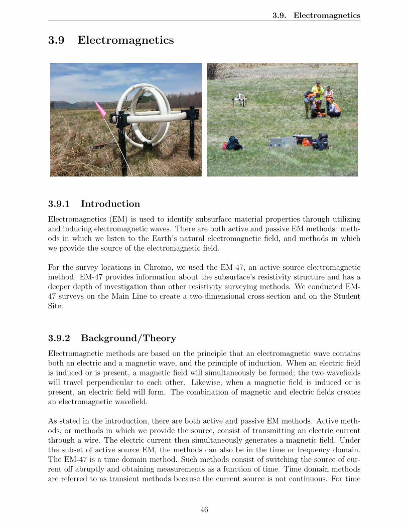
3.9. Electromagnetics
3.9 Electromagnetics
3.9.1 Introduction
Electromagnetics (EM) is used to identify subsurface material properties through utilizingand inducing electromagnetic waves. There are both active and passive EM methods: meth-ods in which we listen to the Earth’s natural electromagnetic field, and methods in whichwe provide the source of the electromagnetic field.
For the survey locations in Chromo, we used the EM-47, an active source electromagneticmethod. EM-47 provides information about the subsurface’s resistivity structure and has adeeper depth of investigation than other resistivity surveying methods. We conducted EM-47 surveys on the Main Line to create a two-dimensional cross-section and on the StudentSite.
3.9.2 Background/Theory
Electromagnetic methods are based on the principle that an electromagnetic wave containsboth an electric and a magnetic wave, and the principle of induction. When an electric fieldis induced or is present, a magnetic field will simultaneously be formed; the two wavefieldswill travel perpendicular to each other. Likewise, when a magnetic field is induced or ispresent, an electric field will form. The combination of magnetic and electric fields createsan electromagnetic wavefield.
As stated in the introduction, there are both active and passive EM methods. Active meth-ods, or methods in which we provide the source, consist of transmitting an electric currentthrough a wire. The electric current then simultaneously generates a magnetic field. Underthe subset of active source EM, the methods can also be in the time or frequency domain.The EM-47 is a time domain method. Such methods consist of switching the source of cur-rent off abruptly and obtaining measurements as a function of time. Time domain methodsare referred to as transient methods because the current source is not continuous. For time
46

3.9. Electromagnetics
domain electromagnetic methods, a constant frequency is used for each measurement. How-ever, different frequencies are used for different measurements and provide a variety of depthsof penetration. Lower frequencies correspond to deeper penetration and higher frequenciescorrespond to shallower penetration.
For frequency domain methods the current is transmitted at a certain frequency in a contin-uous sinusoidal wave. Electromagnetics surveys were not conducted using frequency domainelectromagnetic methods in Chromo, however magnetotellurics surveys were conducted us-ing frequency domain methods [32].
Equations 3.13 - 3.14 form the basis of electromagnetic theory. Ampere’s law, Equation3.13, states that an electric current generates an associated magnetic field that curls aroundthe line of current (meaning the electric and magnetic fields are perpendicular). In Ampere’slaw, B represents the magnetic field, µ represents the magnetic permeability, and J repre-sents the current density.
∇×B = µ0J (3.13)
Faraday’s law of induction is seen in Equation 3.14. Equation 3.14 states that a changingmagnetic flux (magnetic field passing though an area) produces an electromotive force (emf)which is measured in voltage. However, charges want to stay in the lowest energy state, sothere is resistance against the change, as demonstrated by the negative sign (Lenz’s Law).In Faraday’s law, ε represents the electromotive force, and ΦB represents the magnetic flux.
ε = −∂ΦB
∂t(3.14)
In the context of time domain EM and the EM-47 setup specifically, a battery transmits
current through a wire, creating a magnetic field as defined by Equation 3.13. The sourceof current is then abruptly turned off thus changing the magnetic field passing through theground which constitutes as a time varying magnetic flux. From Equation 3.14, this timevarying magnetic flux generates a voltage in the subsurface. From this induced voltage, elec-trons in the Earth are forced to move, therefore creating secondary currents known as eddycurrents [41]. Again from Equation 3.13, the eddy currents set up a secondary magneticfield. As the eddy currents decay in the Earth the secondary magnetic field changes withtime. Another loop of wire known as the receiver is set up on the surface to record thechanging flux induced by the decay of the eddy currents as a function of time. This decayin magnetic flux is recorded in voltage as the changing magnetic flux of the secondary mag-netic field induces an emf in the receiver according to Faraday’s Law. The rate of decay ofthe secondary magnetic flux through the receiver provides information about the resistivitystructure of the subsurface. A flowchart detailing the above concepts can be seen in Figure3.14.
If the measured voltage decays rapidly with time, the subsurface is likely to be resistivebecause current flows in the path of least resistance. Similarly, if the measured voltage de-cays slowly with time, the subsurface is likely to be conductive.
47

3.9. Electromagnetics
Figure 3.14: Flow chart demonstrating how electric and magnetic fields are induced andmeasured using electromagnetics.
Figures 3.15 and 3.16 are diagrams showing the schematics of a ground-based time domainEM survey. Figure 3.15 is a two dimensional diagram showing the magnetic field producedby the transmitting wire of current and the eddy currents induced by the changing magneticfield. Figure 3.16 demonstrates in three dimensions the induced eddy current rings as theyprogress down into the subsurface at later times [41]. Although data from low frequencyelectromagnetic waves images deeper, this data is also low resolution. More measurementsare taken over longer periods of time in order to increase the signal to noise ratio. Moremeasurements over longer time periods are stacked to reduce the amount of random noiseand create the highest resolution image possible. Survey parameters used in our surveys aswell as the set up for the EM-47 can be found in the appendix.
Figure 3.15: Two fimensional example of electric and magnetic field induction as used intime domain electromagnetic methods. [17]
48

3.9. Electromagnetics
Figure 3.16: Diagram of current diffusivity into subsurface as generated by an EM-47Survey. [24]
49

3.10. Magnetotellurics
3.10 Magnetotellurics
3.10.1 Introduction
Magnetotelluric (MT) surveys are used to image the conductivity structure of the Earth. Wealso used magnetotellurics to aid in mapping of fluid flow pathways in the geothermal systeminvestigation. This passive electromagnetic method can image up to hundreds of kilometersdeep and has the greatest depth of investigation of all electromagnetic methods. MT is ca-pable of greater depths of investigation because it can detect very low frequencies comparedto other electromagnetic methods. Fluid flow pathways contain water with charged particlesand have relatively higher conductivity than surrounding lithology, making them an idealtarget for MT surveys. MT data is interpreted in conjunction with other geophysical surveysin order to optimize accuracy.
Using known geology, we can predict what we should expect from an MT survey and whatwe can expect from the inversion. The geology consists of an anticline with overlying shaleand sandstone with a basement Precambrian rock. Therefore, we should expect a moreconductive top layer with a resistive bottom dipping towards the east. We can also lookat known values of resistivities for certain rock types to estimate the general magnitudesof resistivities for the surveys. The Precambrian rock should have a resistivity between1000-100000 Ω*m, sandstone ranges around 100 Ω*m, and shale should have a magnitudearound 10 Ω*m. The shale is interbedded with limestone which should cause an increasein resistivity[19]. Therefore, we may not be able to detect the interface between the shaleand sandstone. Additionally, the sandstone is extremely thin compared to the total depthof penetration, indicating that we may not be able to observe the interface between the layers.
3.10.2 Background/Theory
Magnetotellurics is used to characterize the geo-electrical structure of the subsurface. Solarwinds and distant lightning strikes charge particles in the ionosphere and create large-scaleionospheric current systems. These events produce natural electromagnetic waves whichpropagate towards the Earth and serve as a natural source [43]. Natural electromagneticsource fields induce telluric sheets, or natural sheets of current, according to Faraday’s law(Equation 3.15) where E is the electric filed, and B is the magnetic field.
~∇× E = −∂B∂t
(3.15)
Then, Ampere-Maxwell’s law states that any loop of current is associated with a magneticfield which is proportional to the magnitude of current (Equation 3.16). In Ampere-Maxwell’slaw, H is the magnetic flux, j is the current density, and D is the electric flux.
~∇×H = j +∂D
∂t(3.16)
Taking the curl of Faraday’s Law or the Ampere-Maxwell Law allows us to derive a diffusionequation which can be used to discern the conductivity structure of the Earth [43]. For a
50

3.10. Magnetotellurics
more in depth proof of the diffusion equation see Appendix. Magnetotellurics measures theelectric and magnetic fields corresponding to telluric sheets with four electrodes and two orthree magnetometers oriented in orthogonal directions that are connected to a console thatrecords the data and can apply gains (a method to minimize noise). These measurements areused to calculate the electrical impedance, phase, and apparent resistivity in the frequencydomain. Measurements are volumetric soundings, which yield volumetric averages of theconductivity structure that are approximated as 1-D profiles. A true resistivity structure isinverted with the calculated apparent resistivity and phase, and the impedance tensor is alsoused to provide information on the dimensionality of the conductivity structure. Apparentresistivity is defined as the average resistivity of a uniform half-space. Phase correspondsto the time necessary for electromagnetic waves to diffuse through the subsurface, and theimpedance tensor represents the ratio of electric and magnetic fields in various directions.For more information on the calculations and theory behind apparent resistivity, phase, andthe impedance tensor see the Appendix. Assumptions made in MT surveying are outlinedin the Appendix as well. Magnetotellurics can image depths of approximately 600 km andmay yield valuable information for geological and geothermal investigations where targetsare characterized by conductivity contrasts [43].
51

3.11. Ground Penetrating Radar
3.11 Ground Penetrating Radar
3.11.1 Introduction
Ground penetrating radar (GPR) is a high resolution, active source, geophysical investiga-tion technique utilizing reflections from electromagnetic waves that are sent into the ground.The primary objective of GPR is to investigate the shallow section of subsurface geologyand identify buried material. Ground penetrating radar puts electromagnetic waves intothe subsurface and the waves react to changes in materials’ different electrical properties.Similar to seismic surveying methods, GPR penetrates waves into the ground and listens forreflections, refractions, and diffractions that are sent back to the surface. Through GPR,we detect changes in electrical properties: dielectric permittivity and electrical conductivity.The GPR instrument consists of a transmitter and receiver antenna on the surface. Thetransmitter antenna propagates electromagnetic waves into the ground and the receiver lis-tens for the electromagnetic wave to come back to the surface.
At our survey locations in Chromo, we conducted a GPR survey over the Main Line and theStudent Site in order to understand and locate the transition between the soil interval andthe underlying rock layer. We also used GPR to see many common subsurface objects such aspipelines, culverts, buried cables, etc. GPR also allows us to derive accurate depth estimates.
3.11.2 Background/Theory
GPR detects changes in electrical properties of the shallow subsurface. It transmits elec-tromagnetic waves in the range between 10MHz and 4 GHz into the ground. Theoretically,transmission energy is independent of frequency when using radar frequencies for a numberof materials. However, in reality, if the frequency is below 1 MHz, velocities and frequenciesboth decrease together. Transmission velocity is the key element utilized in the interpreta-tion. When we identify the electromagnetic wave velocity, we can then identify the permit-tivity of the material.
The electromagnetic wave travels from a transmitting antenna into the subsurface mate-rial. The wave continues to travel until it reaches a material that has different electricalproperties from the surrounding medium. At that point, the wave will be scattered back tothe surface into the receiving antenna, and then recorded on the digital storage device forlater interpretation.
Electromagnetic waves travel at specific velocities that are determined primarily by the per-mittivity of material. The relationship between the wave velocity and material properties isthe fundamental basis for using GPR to investigate the subsurface. In other words, the ve-locity is different between materials with different electrical properties, and the signal passedthrough two materials with different electrical properties over the same distance will arriveat different times. The common unit for electromagnetic wave travel time is nano second(ns). Travel time for an electromagnetic wave in space is 3.33 ns/m. Travel time of a wavein Earth material is always greater than 3.33 ns/m.
Electromagnetic waves obey Maxwell’s equations regarding electric and magnetic fields.
52

3.11. Ground Penetrating Radar
Figure 3.17: Transmitted electromagnetic wavefront scattered from a buried objected witha contrasting permittivity. Here, permittivity of the host media is ε1 and the permittivityof the buried object is ε2
However, several assumptions are made in GPR work. First, we assume that the relativemagnetic permeability (µ) of the ground is homogeneous. We assume that the reflection,dispersion (scatter), and attenuation of the transmitted EM wave are resulted from changein conductivity (σ) and the relative electric permittivity (ε). Relative electric permittivitydetermines the ability of the medium to transmit an electric field. We also assume that theparameters above are scalar quantities.
There are four main types of scattering of transmitted electromagnetic waves at the inter-face between a material and the surrounding medium. There is specular reflection scattering,diffraction scattering, resonant scattering, and refraction scattering. When the electromag-netic wave reaches an interface, it scatters the energy according to the shape, roughness, andthe electrical property contrast between the interested objected and surrounding medium.Part of the energy is reflected back to the surface and some energy is reflected through thematerial. This phenomenon obeys Snell’s law as demonstrated in Equation 3.17.
v1v2
=sinφ1
sinφ2
(3.17)
53

3.11. Ground Penetrating Radar
Where, v1 and v2 are the velocities of the wave through the upper and lower materials, re-spectively and φ1 and φ2 are the angles of the raypath for the incident and refracted waves,respectively.
In our surveys in Chromo, GPR measurements were observed in the moving mode, meaningthat the transmitter and receiver antennas were kept at a fixed distance and moving contin-uously. This mode is advantageous for quick data acquisition.
Recorded traces are displayed as a subsurface cross section instantaneously on the visualdisplay, with the horizontal axis representing distance and the vertical axis representingtwo-way travel time of the electromagnetic wave. We can use the travel time to convert thetime to depth if we know the velocity or permittivity.
GPR equipment consists of the two antennas, the accompanying electronics and the record-ing device with visual display screen. For moving mode operation, all of the electronicsare located in one box. GPR data are recorded digitally. Field filtering may be applied toremove noise, however the majority of processing is completed after acquisition is complete.
54

3.12. Hammer Seismic
3.12 Hammer Seismic
3.12.1 Introduction
Shallow seismic techniques were applied at the Main Line survey, around Stinking springs,and the Student Site in order to study and create further understanding of the geothermalsystem in Chromo, Colorado. For all the surveys, we used a sledgehammer and a metal plateas the tool to apply acoustic energy into the Earth. Two type of seismic waves, P-wavesand S waves, were generated and transmitted into the subsurface. While hammer seismichas shallow depths of penetration when compared to our vibroseis survey, we were able tocollect unique data sets in locations more difficult to traverse and collect shear wave data.
3.12.2 Background/Theory
As described above, there are two types of seismic waves generated and recorded in ourhammer seismic surveys.
1. P-wavesP-waves (Primary wave) or compressional waves, travel faster than their S-wave coun-terparts. Particle motion in P waves moves the same direction that the wave energytravels. The velocity of P-waves is given by
Vp =
√K + 4
3µ
ρ(3.18)
where K is the bulk modulusµ is the shear modulusρ is the mass density of the material through which the wave is propagating.
Because P-wave velocity is constrained by both the bulk and shear modulus, P-wavesare able to travel through both solid rock frames and fluids.
2. S-wavesS waves are slower than P-waves. Particle motion in S waves moves perpendicular tothe direction of the wave energy traveling. The velocity of S-waves is given by
Vs =
õ
ρ(3.19)
where µ is the shear modulusρ is the mass density of the material through which the wave is propagating.
Because S-wave velocity is only constrained by the shear modulus, S-waves can notpropagate through fluids.
55
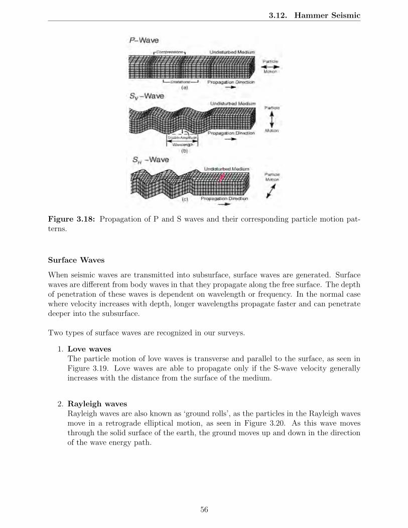
3.12. Hammer Seismic
Figure 3.18: Propagation of P and S waves and their corresponding particle motion pat-terns.
Surface Waves
When seismic waves are transmitted into subsurface, surface waves are generated. Surfacewaves are different from body waves in that they propagate along the free surface. The depthof penetration of these waves is dependent on wavelength or frequency. In the normal casewhere velocity increases with depth, longer wavelengths propagate faster and can penetratedeeper into the subsurface.
Two types of surface waves are recognized in our surveys.
1. Love wavesThe particle motion of love waves is transverse and parallel to the surface, as seen inFigure 3.19. Love waves are able to propagate only if the S-wave velocity generallyincreases with the distance from the surface of the medium.
2. Rayleigh wavesRayleigh waves are also known as ‘ground rolls’, as the particles in the Rayleigh wavesmove in a retrograde elliptical motion, as seen in Figure 3.20. As this wave movesthrough the solid surface of the earth, the ground moves up and down in the directionof the wave energy path.
56

3.12. Hammer Seismic
Figure 3.19: Love wave propagation.
Figure 3.20: Rayleigh wave propagation
Hammer Seismic Acquisition
As the P and S waves penetrate into the Earth, some waves travel along specific subsurfacegeologic boundaries before being refracted back to the surface. We used refraction methodsto calculate seismic velocity and eventually the depth of layers in subsurface. Refractiontheory and processing can be seen in the hammer seismic processing and Appendix sections.
In order to acquire the seismic refraction data, we have both a source and series of re-ceivers. In our surveys we used a sledgehammer striking a metal plate to create the acousticenergy, both P and S wave. Waves are transmitted to the subsurface and propagated throughgeologic boundaries and layers, the refracted back to the ground receivers. Most of the time,we created created several shots at the same location and stacked them together in order toincrease signal-to-noise ratio.
The receivers, called ‘geophones’, receive acoustic energy refracted back from subsurface,sent them to a digitizing unit and eventually to the field recording unit. The recorded datarecords the reflections and refractions from the subsurface of all the waves recorded above.We laid down geophones in a line that spanned the target area of investigation The geophonespacing could be adjusted based on the survey design goals to optimize the data collected.However, while bigger spacing covers a larger area, the resolution decreases. Different setsof geophones, P-wave or S-wave, were used to focus in on a particular type of wave energydepending on the goals of the survey. We collected both sets of data at our survey locations.
57

3.13. Deep Seismic
3.13 Deep Seismic
3.13.1 Introduction
The seismic method is effective for unraveling the geological structure of the Chromo An-ticline because it relies on reflections that come from the rock layer impedance contrasts(See Appendix (impedance contrast)). Unlike other methods, seismic is the closest proxyfor actual geologic boundaries because it relies on acoustic reflections that almost alwayscorrelate to lithologic boundaries.
Seismic can be understood to some degree in the context of physical senses such as sight andhearing. Bats use a biological comparative form of seismic, wherein they emit sound pulsesand by listening to the echo and intuitively measuring the arrival time, they can form animage of their surroundings [21]. For sight, humans rely on light which is an electromagneticwave, reflecting off of physical objects. We notice that our vision is manipulated when wepeer into a pool of water, and witness the law of refraction which is described mathemati-cally by the Snell-Descartes Law also known as Snell’s Law (See Appendix (Snell’s Law)).Density contrasts and abrupt differences in structural composition of the rocks cause seismicrays to bend, but also cause a portion of the energy to reflect back to the surface. Batshave a chief advantage when forming their image wherein the sound pulses they emit travelthrough a mostly invariant medium, air, meaning the acoustic wave they emit essentially hasone velocity. If the earth subsurface is invariant we refer to it as isotropic and homogeneousand it becomes relatively easy to process, but this is rarely the case. Herein lies one of thechallenges of the seismic method - determining the correct velocities of the many differentrock layers in the subsurface.
We rely on compositionally differing rock layers in the subsurface to reflect seismic en-ergy back to the surface. Without these layers, the seismic method would be irrelevant asseismic energy would simply propagate through the subsurface until it attenuates, where theenergy of the source essentially goes to zero. We particularly expect to see large reflectionsat sedimentary/igneous rock boundaries, sandstone/shale boundaries, and normal/reversefaults. Seismic was successful in revealing subsurface layers down to nearly 1.7 kilometers(km) along the main line over the Chromo Anticline as well as revealing a large thrust faultwith nearly 1000 meters of vertical displacement.
Sponsor Roles
While high quality seismic data is paramount in many geophysical surveys, it is also one ofthe most complex and expensive methods to carry out. It requires high-energy sources capa-ble of displacing the subsurface particles (only slightly but on a large scale), and thousands ofrecorders (known as ‘geophones’) all placed methodically in close proximity to one another.For our seismic survey, two 63,000 lb ’Vibroseis’ trucks were supplied by CGG Houston,TX (headquartered in France) who also supplied personnel to maintain and operate them.Sercel, a branch of CGG, also provided personnel to help design our initial seismic surveyand ensure the collected data was satisfactory.
The seismic survey is controlled in an enclosure, known as the ‘doghouse’ and containsthe data recording computers. An ‘observer’ monitors the doghouse, writes computer scripts
58

3.13. Deep Seismic
for geometrically dictating the seismic survey, and ensures that parameters such as sufficientcoupling occur between the Vibroseis truck and the ground. Sercel provided personnel tocontrol the doghouse and educate students in the process with one-on-one training, allowingthe students to begin seismic sweeps and monitor the parameters under their guidance andsupervision.
3.13.2 Background/Theory
The seismic method has its roots in classical Newtonian physics. Impact forces applied to thesubsurface result in small accelerations that propagate through the earth in wave formation.Impedance contrasts in the subsurface create different wave types such as reflections, refrac-tions, and diffractions that propagate back up to the surface (See Appendix (Seismic WaveTypes)). According to Fermat’s principle (See Appendix (Fermat’s and Hygens’ Principles))we can derive that the reflected ray has an angle equivalent to the angle of incidence, whichassists in configuring travel times and velocities. If we know something about the velocityat which seismic waves travel through different rocks, we can unravel the timing that thereflected rays arrive back at the surface after the source goes off (See Appendix (velocityappendix)).
The times at which these back propagated waves reach the surface are closely recordedwithin milliseconds using ‘geophones’ (See Appendix (geophones)). Artificial propagation ofthese waves in the subsurface requires a source, however to obtain data of respectable qualitywe must ensure the source is meticulously controlled. The type of source that often timesgives the best data quality is a vibroseis truck, which puts energy into the earth at varyingfrequencies. Certain parameters are chosen based on the geology of the area. This willdetermine the particular wavefield that will be generated by a vibroseis truck. Subsurfacecharacteristics such as the shape and type of rock formations, and depth of imaging desiredall play a role in helping determine the type, bandwidth, and timespan of parameters usedin a survey. The process of determining parameters for seismic acquisition is known as thesweep test. Higher frequencies in a sweep attenuate quickly and are unable to give us infor-mation on deeper geologic features, however they can provide high-resolution images. Lowerfrequencies have the advantage of depth, but otherwise are burdened by lower resolution.
Once the seismic survey is set up, and sweep parameters are determined, seismic data isrecorded along a line of receivers which must be sorted into particular configurations usefulfor processing and forming an image. We utilized the common midpoint (CMP) gather, aconfiguration in which the data are sorted into linearly increasing offsets between the sourceand receiver while the point of reflection is held constant (See Appendix (CMP’s)). The mainadvantage of any gather of data in seismic acquisition is its ability to highlight importantsignals over irrelevant ones which aids in seismic processing and producing a usable seismicimage which is known as a stack.
59
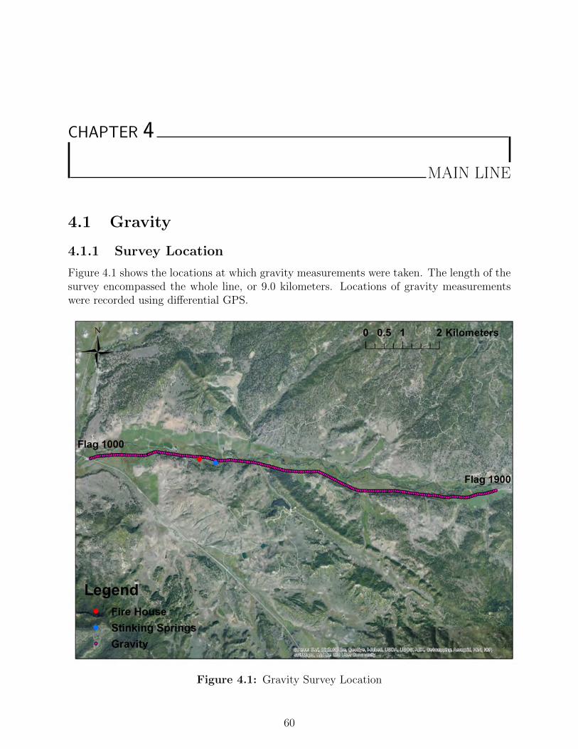
CHAPTER 4
MAIN LINE
4.1 Gravity
4.1.1 Survey Location
Figure 4.1 shows the locations at which gravity measurements were taken. The length of thesurvey encompassed the whole line, or 9.0 kilometers. Locations of gravity measurementswere recorded using differential GPS.
Figure 4.1: Gravity Survey Location
60

4.2. Processing
4.1.2 Survey Design
Along the Main Line we took measurements every four flags beginning at flag 1000. We took225 measurements along the line. For each location along the survey, the gravimeter wasleveled on the side of the road and sampled three measurements for thirty seconds each. Wedecided to measure every four flags due to the amount of time it takes to level the gravimeterand the time needed to complete the three readings at each station. Every day two differentteams, a morning group and an afternoon group, took gravity measurements along the mainline. Base station readings were taken at the beginning and end of each teams’ survey.
4.2 Processing
4.2.1 Corrections
In order to extract the true anomalies of interest from the data, effects from tidal drift,elevation changes, and gravity fields due to background mass must be removed in order toprevent false anomalies from skewing the geologic interpretation. Applying alterations tothe raw data such as the Free-Air and the Bouger correction reveals density variations thatprovide information about the subsurface relevant to our survey.
Before corrections were applied, pre-processing was applied to the data. This consistedof reviewing the raw data and removing outlying measurements. For example, if one of thethree measurements at a station deviated from the other two by 10µGal, it was deleted. Theremaining measurements were averaged together to give one measurement at each station.
Tidal/Drift Correction
Gravitational forces from the moon and sun affect the gravitational field of the earth, pro-ducing gravity variations unrelated to local geology. These forces vary throughout the daydue to Earth’s rotation, changing the locations of the moon and sun relative to the earth.These background variations are removed by using the base station readings taken through-out the day. The base station acts as a monitor of the gravity changes that occur while thesurvey is being conducted. We assume that the changes in gravity over time follows a linearpattern from when the first base station measurement is recorded to when the next basestation measurement is recorded. From this assumption, we can use Equation 4.1 to solvefor the gravity measurements with tidal affects from the moon and sun removed, where g1and t1 are the gravity and time at the initial base station, g2 and t2 refer to the final basestation, and g and t refer to measurements made in the field.
gD = g − (t− t1)g2 − g1t2 − t1
(4.1)
61
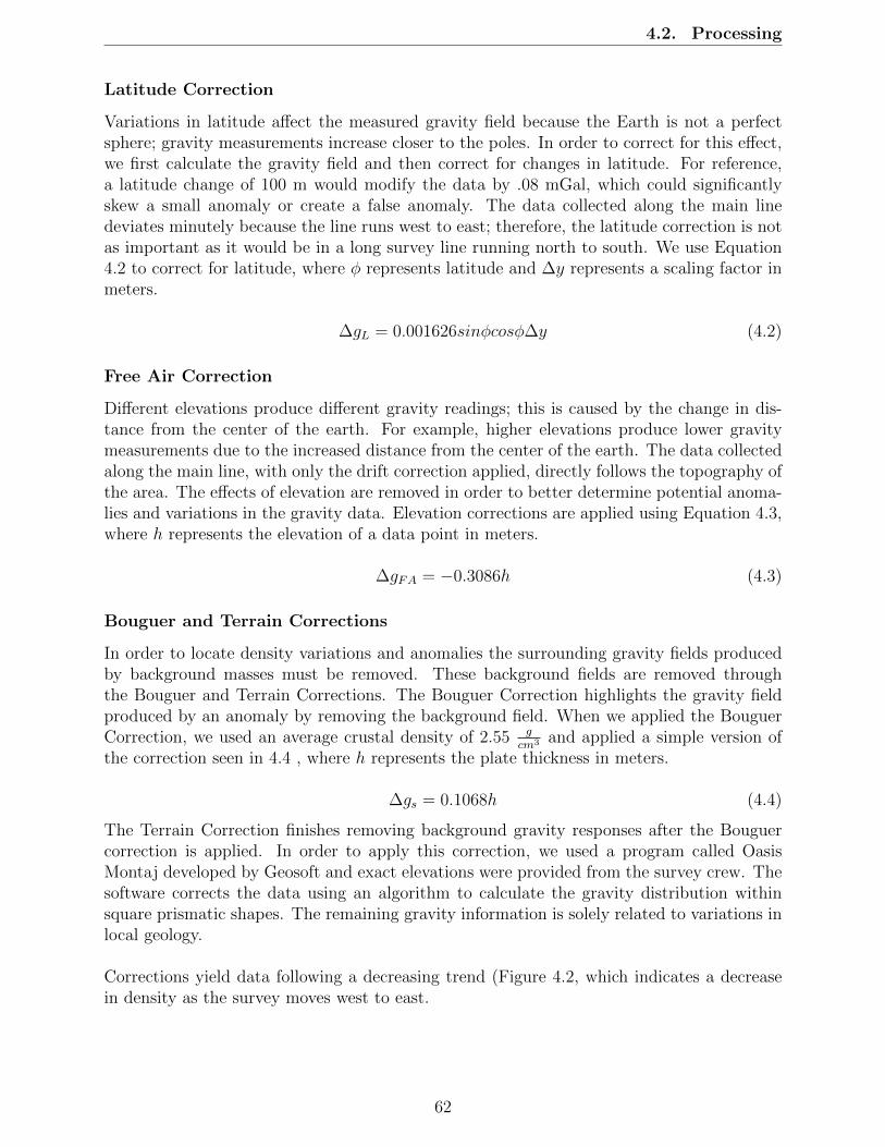
4.2. Processing
Latitude Correction
Variations in latitude affect the measured gravity field because the Earth is not a perfectsphere; gravity measurements increase closer to the poles. In order to correct for this effect,we first calculate the gravity field and then correct for changes in latitude. For reference,a latitude change of 100 m would modify the data by .08 mGal, which could significantlyskew a small anomaly or create a false anomaly. The data collected along the main linedeviates minutely because the line runs west to east; therefore, the latitude correction is notas important as it would be in a long survey line running north to south. We use Equation4.2 to correct for latitude, where φ represents latitude and ∆y represents a scaling factor inmeters.
∆gL = 0.001626sinφcosφ∆y (4.2)
Free Air Correction
Different elevations produce different gravity readings; this is caused by the change in dis-tance from the center of the earth. For example, higher elevations produce lower gravitymeasurements due to the increased distance from the center of the earth. The data collectedalong the main line, with only the drift correction applied, directly follows the topography ofthe area. The effects of elevation are removed in order to better determine potential anoma-lies and variations in the gravity data. Elevation corrections are applied using Equation 4.3,where h represents the elevation of a data point in meters.
∆gFA = −0.3086h (4.3)
Bouguer and Terrain Corrections
In order to locate density variations and anomalies the surrounding gravity fields producedby background masses must be removed. These background fields are removed throughthe Bouguer and Terrain Corrections. The Bouguer Correction highlights the gravity fieldproduced by an anomaly by removing the background field. When we applied the BouguerCorrection, we used an average crustal density of 2.55 g
cm3 and applied a simple version ofthe correction seen in 4.4 , where h represents the plate thickness in meters.
∆gs = 0.1068h (4.4)
The Terrain Correction finishes removing background gravity responses after the Bouguercorrection is applied. In order to apply this correction, we used a program called OasisMontaj developed by Geosoft and exact elevations were provided from the survey crew. Thesoftware corrects the data using an algorithm to calculate the gravity distribution withinsquare prismatic shapes. The remaining gravity information is solely related to variations inlocal geology.
Corrections yield data following a decreasing trend (Figure 4.2, which indicates a decreasein density as the survey moves west to east.
62
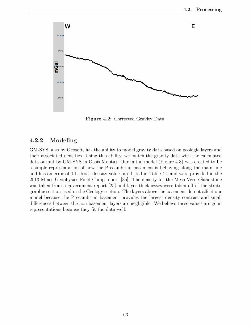
4.2. Processing
Figure 4.2: Corrected Gravity Data.
4.2.2 Modeling
GM-SYS, also by Geosoft, has the ability to model gravity data based on geologic layers andtheir associated densities. Using this ability, we match the gravity data with the calculateddata output by GM-SYS in Oasis Montaj. Our initial model (Figure 4.3) was created to bea simple representation of how the Precambrian basement is behaving along the main lineand has an error of 0.1. Rock density values are listed in Table 4.1 and were provided in the2013 Mines Geophysics Field Camp report [35]. The density for the Mesa Verde Sandstonewas taken from a government report [25] and layer thicknesses were taken off of the strati-graphic section used in the Geology section. The layers above the basement do not affect ourmodel because the Precambrian basement provides the largest density contrast and smalldifferences between the non-basement layers are negligible. We believe these values are goodrepresentations because they fit the data well.
63

4.2. Processing
Table 4.1: Density values used for geology-guided gravity model.
Geologic layer Density (g × cm−3)Mesa Verde 2.59Mancos 2.55Dakota 2.61Morrison 2.52Wanakah 2.63Entrada 2.50Precambrian basement 2.80
Figure 4.3: Geology-Guided Gravity Model.
Considering that gravity primarily picks up on the density contrast of the basement, ourmodel requires the offset produced by the presence of a fault that penetrates down to thePrecambrian basement. Our data could have supported either solution of a reverse fault, aspictured, or a normal fault. The bulge to the east of the fault is a good fit to our data sincethat area required an increase in density. The presence of a fracture zone is also supportedby the gravity data, although gravity cannot pick out subtleties in the fracture zone.
Before integration with the seismic section, we set out to get as accurate density values aspossible. Table 4.2 shows the density values that we were able to obtain through researchingliterature. However, the values for the Dakota and Morrison are uncharacteristically low forformations of sandstone and shale. This could be due to the fractures within the units maycause a decrease in density. However, the values that we end up using in our seismic-guidedmodel seem more realistic (Table 4.3).
64

4.2. Processing
Table 4.2: Density values from literature
Geologic layer Density (g × cm−3)Mesa Verde 2.59Mancos 2.63Dakota 2.38Morrison 2.32
After integration with deep seismic results, we refine our model, which is seen in Figure 4.4.The major differences in our model are that the throw of the fault is much larger (nearly1000m rather than 300m), the Fountain Formation is present on the east side of the fault,and the fracture zone is extended to the location of Stinking Springs in our new model. Thefault is still modeled as a reverse fault and the thicknesses of the layers remain consistenteast to west. We adjust the density values to fit the data better, which are seen in Table4.3. Although these can vary, we believe these values are the more accurate representationof the subsurface. The error in this model is 0.113.
Table 4.3: Density values used for seismic-guided gravity model
Geologic layer Density (g × cm−3)Fractured shale 2.61Mesa Verde 2.70Mancos 2.65Dakota 2.67Morrison 2.64Entrada and Todilto 2.64Fountain 2.68Precambrian basement 2.80
65
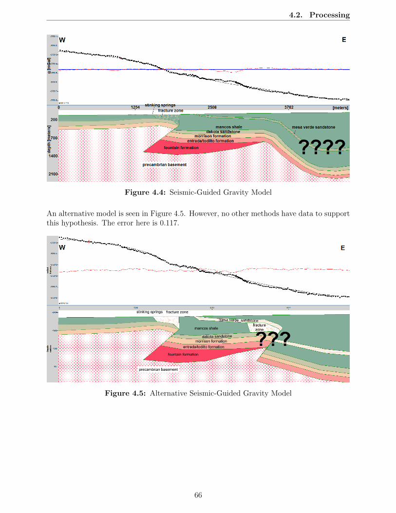
4.2. Processing
Figure 4.4: Seismic-Guided Gravity Model
An alternative model is seen in Figure 4.5. However, no other methods have data to supportthis hypothesis. The error here is 0.117.
Figure 4.5: Alternative Seismic-Guided Gravity Model
66

4.3. Interpretation/Discussion
4.3 Interpretation/Discussion
When processing gravity data, it is important to realize that models produced are non-unique. Therefore, it is important to guide the model by using knowledge procured fromgeology and seismic data. Our preliminary model guided solely from geologic knowledge ofthe area, as seen in Figure 4.3, supports the presence of a large reverse fault just east of thetop of the Archuleta Anticline. Gravity is the only method that surveyed the far easternhalf of the Main Line with quality data; instead of over-interpreting the system, we createda model that slightly raises the Precambrian basement for about 1.0 km and continues todip as expected in an anticlinal feature. We input a fracture zone around the anticlinal areain order to fit the calculated data to the observed. The fracture zone is a slightly less densearea which changes the calculated data by 120 mGal.
The seismic guided model extends the fault and shows an increased fault angle. The factthat the throw of the fault was interpreted to be much larger than before means either thesedimentary layers thicken significantly to the east, or there is another layer present thattapers off. The latter scenario is more feasible geologically and tectonically, and is explainedin-depth in the Main Line Integration section. Our gravity model supports the presence ofthe Fountain Formation, but the Precambrian basement may be coming up more to the west.The eastern part of our section still holds many uncertainties, again because the seismic linedid not extend very far east. One alternative solution that may fit the data is the presenceof a second fault on the east side, as seen in Figure 4.5. Data from seismic would be requiredto support this hypothesis, so this area is a possible site of future geophysical data acquisition.
The Mesa Verde sandstone location was inserted into the model using strikes and dips fromoutcrops in the area, so the location of the layer did not change between the geology-guidedand seismic-guided figures.
4.4 Sources of Error/Uncertainty
After corrections are applied, there are still several factors that can affect gravity measure-ments. If the gravimeter is not finely leveled or not placed firmly into the ground inconsisten-cies may arise in the data. Additionally, cars passing by the gravimeter while measurementsare being taken can shake the ground in addition to producing their own large gravity field,both of which cause errors in the data. Wind also causes erroneous gravity data and somemeasurements had to be redone due to strong gusts. Additionally, several people working onthe line may have caused errors in the gravity data by shaking the ground or being too closeto the gravimeter while measurements were being taken. The inversion produced by evenslightly flawed data will be inaccurate, which may explain why our initial geology guidedmodel is so different from our seismic guided model. The solutions produced are non-unique,so many of the interpretations are subjective.
Errors can also arise from processing. We are confident that the drift correction was ac-curate, since we can see in the data if gravity measurements do not match up station tostation. The latitude correction does not drastically affect the data because our data wascollected west to east. Problems could have risen in the Bouguer and Terrain correctionsdue to the assumption of an average crustal density of 2.55 g × cm−3.
67

4.5. Conclusion
As mentioned in the Discussion, gravity models have many non-unique solutions and modelsmust be guided by other methods: geophysical, geological, or both. As a result, the modelsproduced are not guaranteed to be a completely accurate representations of the subsurface.Fitting multiple methods’ data in our interpretation will of course not be accurate accordingto each method, but the integrated model will give us the best picture of what is happeningin the subsurface.
4.5 Conclusion
Gravity is an important method for imaging deep structural features. Although it is moredifficult to pick out finer features with gravity, when combined with seismic interpretation,these two methods have the best depth of investigation and resolution for imaging the Pre-cambrian basement on the Main Line. Gravity can also be integrated with other methodsto support working hypotheses. Geologic and tectonic knowledge played a large role in thegravity model and interpretation, so integration of both geophysical and geologic methodsis important when determining an accurate representation of the subsurface.
Gravity supports the presence of a large reverse fault to the east of Stinking Springs, andwe believe the event that formed the Archuleta Arch reactivated the reverse fault to makethe offset larger than it initially was. The fault extends to the Precambrian basement, andmay be a conduit for fluid flow. The presence of a fracture zone is supported by gravity anddocumented by seismic as well as DC resistivity (see Main Line Integration). The presence ofthe Fountain Formation is plausible using the collected gravity data, as the density is similarto the other sandstone layers and the basement must rise in the east before dropping moreto the east. The location of the Mesa Verde sandstone is required by our gravity model,but we are uncertain of why the dip changes dramatically from 55 on surface expressionsto near horizontal in the subsurface.
The ability of gravity to characterize the reverse fault that extends to the basement providesvaluable insight into characterizing a possible conduit for water flow, which is elaboratedmore on in the Main Line Integration section.
Because of the large uncertainty present on the east side of the line, we recommend a seis-mic survey be conducted in order to complete our gravity line in the future. Future dataacquisition may have both gravity and seismic going farther east and making another lineto the north.
68

4.6. Magnetics
4.6 Magnetics
4.6.1 Survey Location
Figure 4.6: A regional map showing the location of the magnetic survey.
The magnetic survey was completed along the 9.0 kilometer long Main Line, running fromwest to east. The Main Line began just north of intersection of Colorado Highway 84 andCounty Road 382 (CR382). The Main Line followed parallel to CR382, one meter to thenorth of the road. Survey flags are located every 10 meters along the entire length of theline.
4.6.2 Survey Design
The magnetics survey consists of two main components: the mobile magnetometer, whichis composed of two cesium vapor magnetometers, and the base station (a proton precessionmagnetometer).
The magnetics survey recorded a point at every flag along the Main Line, taking a read-ing every ten meters. In an attempt to avoid noise from the large metal fences runningalong either side of the road, readings were taken near the center of the road when pos-sible. Two cesium magnetometers were used during the survey, oriented vertical to eachother and the ground. This will result in two sets of data with the bottom magnetometer
69

4.6. Magnetics
being more sensitive to anomalies and noise alike. The top magnetometer will have less noisebut also less sensitivity. Using the discrete mode on the magnetometers, the user manuallytook a reading at each desired location. This is in contrast to continuous mode where theuser simply walks the line and a reading is automatically recorded at a desired time sampling.
The proton precession magnetometer was set to record at one-minute intervals. The purposeof the constant base station measurements is for post processing corrections. The magne-tometer itself was located a few hundred meters south of the fire station in order to minimizeinterference from outside sources.
4.6.3 Processing
Correcting the cesium vapor magnetometer for diurnal magnetic variations was the first stepin the processing of the magnetic data. Earth’s magnetic field varies greatly throughoutthe day, which produces noisy data (Figure 4.7). Correcting for diurnal variation is fairlystraightforward. Each value is correlated to a time for both the proton precession and cesiumvapor magnetometers. The value from the proton precession magnetometer is subtractedfrom the reading gathered by the cesium vapor magnetometer at the closet available time.The values produced are the corrected magnetic values.
Figure 4.7: Plot of the data recorded by the proton precession magnetometer used incorrections
Once the data has been corrected, we performed initial processing in MagMap2000. Most ofthe area near the magnetics survey was littered with potential sources of noise such metalfences, culverts, and power lines. These sources of noise can possibly mask deeper geologicalinformation. To determine the actual anomalous trends, we used a smoothing function withinMagMap2000. The diurnally corrected data can be seen in Figure 4.8, and the smootheddata can be viewed in Figure 4.9. As anticipated, our raw data was extremely noisy makingmultiple iterations of the smoothing function necessary. The smoothed data appears to showthe anomalous trend, but poor plotting quality led to other methods of processing.
70
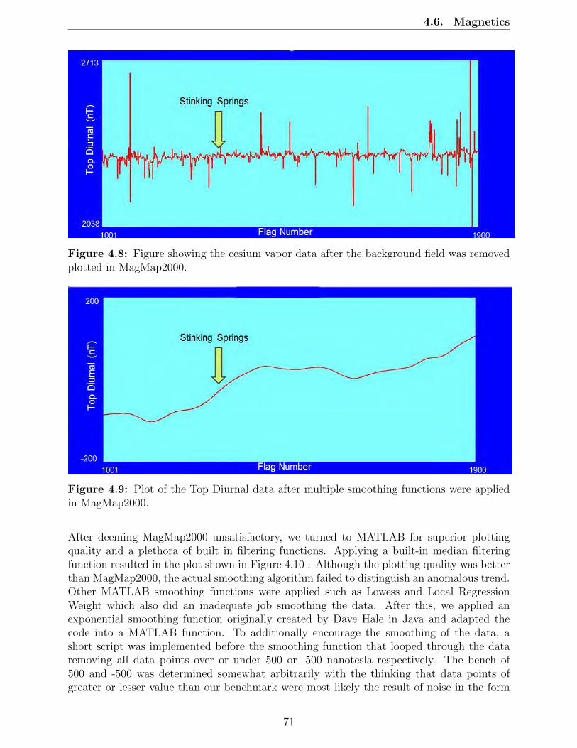
4.6. Magnetics
Figure 4.8: Figure showing the cesium vapor data after the background field was removedplotted in MagMap2000.
Figure 4.9: Plot of the Top Diurnal data after multiple smoothing functions were appliedin MagMap2000.
After deeming MagMap2000 unsatisfactory, we turned to MATLAB for superior plottingquality and a plethora of built in filtering functions. Applying a built-in median filteringfunction resulted in the plot shown in Figure 4.10 . Although the plotting quality was betterthan MagMap2000, the actual smoothing algorithm failed to distinguish an anomalous trend.Other MATLAB smoothing functions were applied such as Lowess and Local RegressionWeight which also did an inadequate job smoothing the data. After this, we applied anexponential smoothing function originally created by Dave Hale in Java and adapted thecode into a MATLAB function. To additionally encourage the smoothing of the data, ashort script was implemented before the smoothing function that looped through the dataremoving all data points over or under 500 or -500 nanotesla respectively. The bench of500 and -500 was determined somewhat arbitrarily with the thinking that data points ofgreater or lesser value than our benchmark were most likely the result of noise in the form
71

4.6. Magnetics
of cultural artifacts. Magnetics data was also imported in a program called Oasis Montage.Oasis Montage is program designed to forward model both magnetics and gravity data withgeologic inputs and output a model of the data that fits the geological inputs. This isespecially useful when attempting to assess the overall validity of the data.
Figure 4.10: Plot of the Top Diurnal data aftera median filtering was applied in MATLAB.
4.6.4 Interpretation
The results from the magnetic data initially appeared to reveal a few useful trends. Thesmoothing algorithm adequately removed obvious sources of noise and left the apparentanomalous field (Figure 4.11). The magnetic field along the Main Line shows an overall up-ward trend from west to east. This could possibly indicate the more magnetic Precambrianbasement being pushed upwards near the anticline in this area. However, the forward mod-eling produced by Oasis Montage yielded less definitive results. The model produced fromthe known geological formations in the area did not produce a close match to the magneticsdata. Approximately the first half of the Main Line data does not correlate with the forwardmodeling. The only way for the predicted data to match the observed data is to incorporateremnant magnetization, but as we do not know the remnant magnetization, we cannot makeany confident interpretations. It is likely that the data is strongly driven by the culturalfeatures in this area, despite attempts to minimize noise by conducting the survey near thecenter of the road.
72

4.6. Magnetics
Figure 4.11: Plot of the Top Diurnal data with various corrections applied. The moreerratic pink lines represent the original data after the de-spiking loop. The green and blacklines represent the data after one and two iterations of the exponential smoothing algorithm,respectively.
Figure 4.12: Plot showing the data fit for the suspected geology of the area. The boldblack line on the top plot represents our collected data, the black line represents data thatwould fit the geology, and the red line is error. Error is 24%.
73

4.6. Magnetics
4.6.5 Sources of Error/Uncertainty
The obvious sources of error and uncertainty result from the abundance of cultural noise nearthe Main Line. Specifically, there was a large metal fence that ran along at least one side ofthe road at almost all times. Additionally, error may have been created during processing.The cutoff value of positive or negative 500 nT was an informed guess, however, it is plausiblethat some of the anomalous data was cut off along with the noise.
4.6.6 Conclusion
Despite efforts to minimize noise, we cannot make any large-scale geologic conclusions fromthe magnetic data gathered. The cultural noise was too prevalent and significantly skewedthe data. However, the magnetics data could still be cross-correlated with GPR data tolocate significant cultural features that could adversely affect other methods such as DCresistivity and various electromagnetic methods. Unfortunately, no greater conclusions couldbe confidently drawn from the data. However, due to time constraints no integration of othermethods were accomplished.
74

4.7. Direct Current Resistivity
4.7 Direct Current Resistivity
4.7.1 Survey Location
The main survey line was set up along County Road 382, running West-East through Chromoand the surrounding area. It covered most of the width of the anticlinal structure beingstudied and crossed over the road beside the Stinking Springs area. Figure 4.13 shows, indark green, the DC line positioned along the main line. The total length of the DC resistivityline was 9,480 meters, with 475 flags spaced 20 meters apart along the south end of CR382.Acquisition for the main DC line was done from East to West (flags 1-475) so as to avoidany sources of noise or error associated with other geophysical methods.
Figure 4.13: Aerial photo of the DC survey line along main line along CR382
4.7.2 Survey Design
In DC resistivity, two current electrodes A and B (source + and sink -) are used to runcurrent through the subsurface, while two potential electrodes M and N measure voltageacross a given distance, shown in Figure 4.14. The current patter will vary according tothe resistivity of the space below an acquisition. Figure 4.14 shows the current flow patternfor a two-dimensional uniform half-space of earth, while Figure 4.15 shows different currentpatterns for simple two-layer Earth scenarios with different distributions of resistivity un-derground. In reality, these scenarios are oversimplifications, but they give a general ideafor how variations in the subsurface resistivity can result in different measurable responsesthat are detectable at the surface.
75

4.7. Direct Current Resistivity
Figure 4.14: AB/MN Electrode set-up [38]
Figure 4.15: Current flow patters for a) uniform halfspace b) two-layer scenario with lowerresistivity on top c) two-layer scenario with lower resistivity below. [33]
76
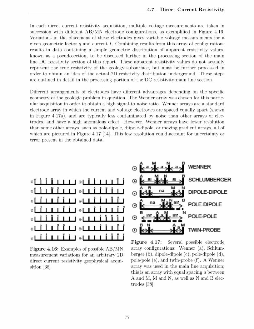
4.7. Direct Current Resistivity
In each direct current resistivity acquisition, multiple voltage measurements are taken insuccession with different AB/MN electrode configurations, as exemplified in Figure 4.16.Variations in the placement of these electrodes gives variable voltage measurements for agiven geometric factor g and current I. Combining results from this array of configurationsresults in data containing a simple geometric distribution of apparent resistivity values,known as a pseudosection, to be discussed further in the processing section of the mainline DC resistivity section of this report. These apparent resistivity values do not actuallyrepresent the true resistivity of the geology subsurface, but must be further processed inorder to obtain an idea of the actual 2D resistivity distribution underground. These stepsare outlined in detail in the processing portion of the DC resistivity main line section.
Different arrangements of electrodes have different advantages depending on the specificgeometry of the geologic problem in question. The Wenner array was chosen for this partic-ular acquisition in order to obtain a high signal-to-noise ratio. Wenner arrays are a standardelectrode array in which the current and voltage electrodes are spaced equally apart (shownin Figure 4.17a), and are typically less contaminated by noise than other arrays of elec-trodes, and have a high anomalous effect. However, Wenner arrays have lower resolutionthan some other arrays, such as pole-dipole, diipole-dipole, or moving gradient arrays, all ofwhich are pictured in Figure 4.17 [14]. This low resolution could account for uncertainty orerror present in the obtained data.
Figure 4.16: Examples of possible AB/MNmeasurement variations for an arbitrary 2Ddirect current resistivity geophysical acqui-sition [38]
Figure 4.17: Several possible electrodearray configurations: Wenner (a), Schlum-berger (b), dipole-dipole (c), pole-dipole (d),pole-pole (e), and twin-probe (f). A Wennerarray was used in the main line acquisition;this is an array with equal spacing a betweenA and M, M and N, as well as N and B elec-trodes [38]
77

4.7. Direct Current Resistivity
Equipment
DC Resistivity measures the voltage, across a certain array of electrodes for a given injectedcurrent to determine subsurface resistivity distributions. Table 4.4 outlines the equipmentused in the 2D DC resistivity main line acquisition that was necessary to successfully carryout a geophysical investigation of the resistivity structure below the surface.
Item PurposeABEM Computer Data storage and collectionBattery Provides power necessary to run current through reels and
electrodes into ground8 reels of takeout cables These transport current from the battery to the electrodes64 metal electrodes Pounded 5 inches into the ground, these direct current running from
battery through the reels into the ground and provide a means bywhich to measure voltage
Alligator clips Connect takeouts on reels to electrodes to transfer currentfrom reel to electrodes
Reel connectors Connect current-carrying reels to one anotherElectrode sensor Determines spacing and location of AM/MN electrodes at
any point during an acquisition
Table 4.4: Required equipment for 2D DC Resistivity acquisition
Parameters
Table 4.5 outlines the parameters used in the DC resistivity mainline acquisition. Furtherdetail can be found in the appendix for DC resistivity.
Parameter ValueArray type WennerElectrode spacing 20 mImposed current 200 mAAcquisition time 0.60 secondsDelay time 0.30 secondsLength of single acquisition 1.26 kmMeasurements per acquisition 472
8 stacks per measurement(stack is cut off if standarddeviation falls under 5 percent)
Total acquisition length 9.5 kmApproximate depth of investigation 220 m
Table 4.5: Parameters used for 2D DC Resistivity mainline acquisition
78
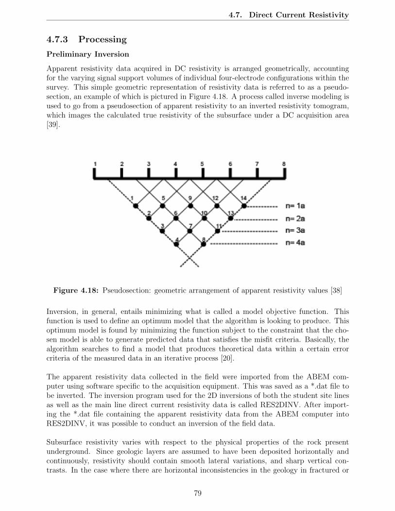
4.7. Direct Current Resistivity
4.7.3 Processing
Preliminary Inversion
Apparent resistivity data acquired in DC resistivity is arranged geometrically, accountingfor the varying signal support volumes of individual four-electrode configurations within thesurvey. This simple geometric representation of resistivity data is referred to as a pseudo-section, an example of which is pictured in Figure 4.18. A process called inverse modeling isused to go from a pseudosection of apparent resistivity to an inverted resistivity tomogram,which images the calculated true resistivity of the subsurface under a DC acquisition area[39].
Figure 4.18: Pseudosection: geometric arrangement of apparent resistivity values [38]
Inversion, in general, entails minimizing what is called a model objective function. Thisfunction is used to define an optimum model that the algorithm is looking to produce. Thisoptimum model is found by minimizing the function subject to the constraint that the cho-sen model is able to generate predicted data that satisfies the misfit criteria. Basically, thealgorithm searches to find a model that produces theoretical data within a certain errorcriteria of the measured data in an iterative process [20].
The apparent resistivity data collected in the field were imported from the ABEM com-puter using software specific to the acquisition equipment. This was saved as a *.dat file tobe inverted. The inversion program used for the 2D inversions of both the student site linesas well as the main line direct current resistivity data is called RES2DINV. After import-ing the *.dat file containing the apparent resistivity data from the ABEM computer intoRES2DINV, it was possible to conduct an inversion of the field data.
Subsurface resistivity varies with respect to the physical properties of the rock presentunderground. Since geologic layers are assumed to have been deposited horizontally andcontinuously, resistivity should contain smooth lateral variations, and sharp vertical con-trasts. In the case where there are horizontal inconsistencies in the geology in fractured or
79

4.7. Direct Current Resistivity
faulted areas, a sharp variation should change the general trend of resistivity from one setof consistent values to another. So, while large, consistent changes in the general trend oflateral resistivity were kept, sharp local jumps, like those marked by the red crosshairs inFigure 4.19 were eliminated from the pseudosection. A built-in function within the program(Exterminate bad data points) was used to manually remove these erroneous data pointsthat were present in the apparent resistivity pseudosections so that the program would av-erage out the exterminated points and generate a revised section. (Figure 4.19).
This process of elimination generates a new pseudosection datafile with revised points.
Figure 4.19: Manual point extermination tool in RES2DINV; anomalous points are selectedand marked with a red crosshair (enhanced with red circle). The program then averages thesepoints out to produce a more smooth resistivity profile.
A least-squares inversion was performed on the resulting datafile with three iterations, sinceadditional iterations were incorporating too much noise and producing far too complicateda model for the known geology of the area. Using a combined inversion, rigid regression, orMarquardt, and smoothness constrained, Occam parameters were incorporated. A standardL2 Norm inversion was carried out to smooth out the data; robust inversion would havecreated less smooth results [14].
Preliminary inversions were inspected and refined using the Root-Mean-Square, or RMS,error tool built in to RES2DINV program. This RMS tool was used to define a percent errorcutoff for the following inversion using a histogram, pictured in Figure 4.20. The histogramcorrelates the measured points from the survey and the calculated theoretical data pointsresulting from the inversion data generated to match the field data. High-error points wereeliminated from the section, as shown in Figure 4.20.
80

4.7. Direct Current Resistivity
Figure 4.20: RMS error histogram with cutoff defined at 12 percent error
After observing the initial inversions, additional parameters were incorporated to refine theinversion process, including topography information, damping factors, and a vertical-to-horizontal ratio of 0.20 to correct for vertical elongation. Initial damping factor was set at0.25, with a minimum of 0.05, setting the first layer at a value of 10.0.
Once a satisfactory preliminary model was obtained in RES2DINV, the corresponding datafile was transferred into Surfer to create a contour plot of the inverted resistivity tomogramon a logarithmic scale using kriging, a spatial interpolation method, rather than value-basedsmoothing. Adjustment of the color scale and the vertical exaggeration were used to bringout desired detail in the image. Upon evaluation of the final preliminary main line inversion(Figure 4.21), a tentative cross-section could be constructed using correlation from EM andSeismic methods. This cross-section could be used to perform image-guided inversion of themain line data, and is pictured in Figure 4.22.
Prospective Method of Processing: Image-guided Inversion
To obtain a highly accurate model, more information can be incorporated into the inversionprocess from other data sources. This is known as image-guided inversion, a process in whichadditional data, such as a cross-section or a migrated seismic section, is used to constrain
81
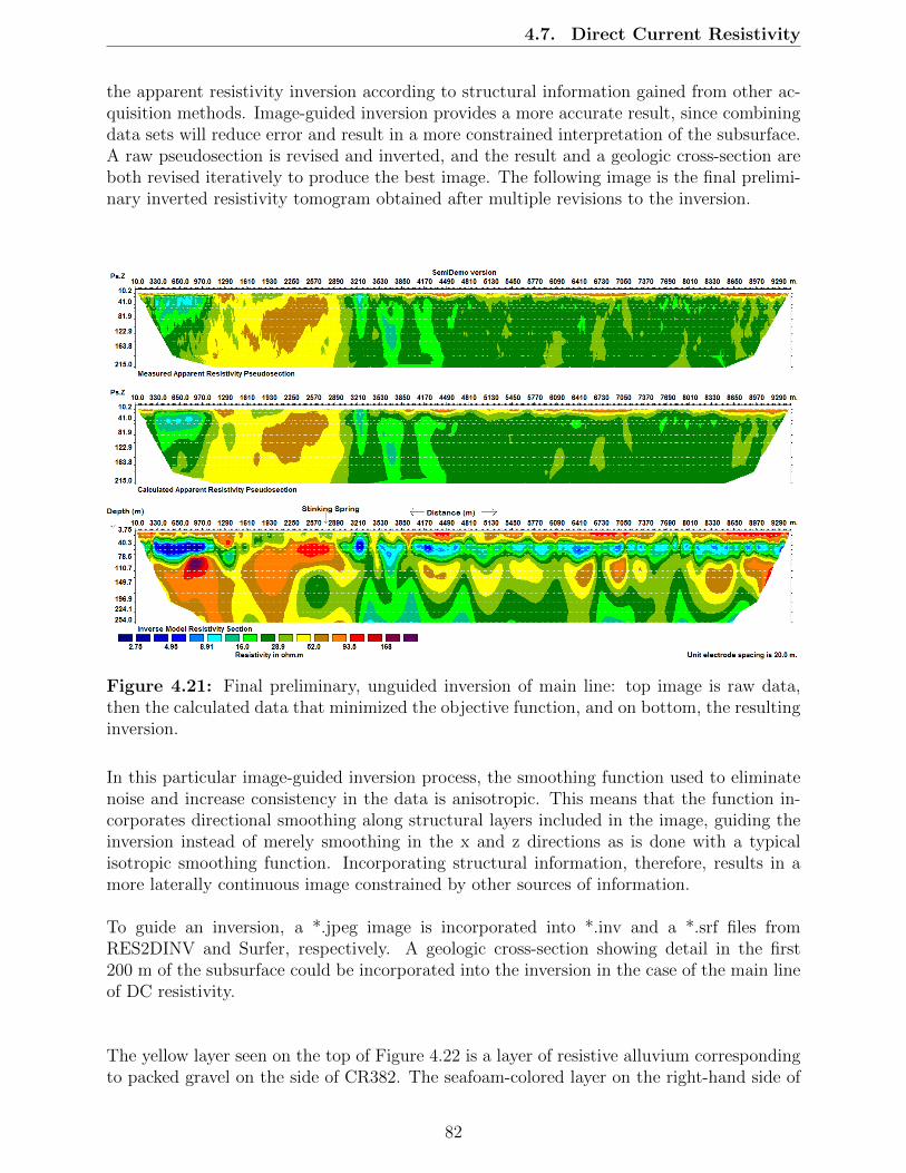
4.7. Direct Current Resistivity
the apparent resistivity inversion according to structural information gained from other ac-quisition methods. Image-guided inversion provides a more accurate result, since combiningdata sets will reduce error and result in a more constrained interpretation of the subsurface.A raw pseudosection is revised and inverted, and the result and a geologic cross-section areboth revised iteratively to produce the best image. The following image is the final prelimi-nary inverted resistivity tomogram obtained after multiple revisions to the inversion.
Figure 4.21: Final preliminary, unguided inversion of main line: top image is raw data,then the calculated data that minimized the objective function, and on bottom, the resultinginversion.
In this particular image-guided inversion process, the smoothing function used to eliminatenoise and increase consistency in the data is anisotropic. This means that the function in-corporates directional smoothing along structural layers included in the image, guiding theinversion instead of merely smoothing in the x and z directions as is done with a typicalisotropic smoothing function. Incorporating structural information, therefore, results in amore laterally continuous image constrained by other sources of information.
To guide an inversion, a *.jpeg image is incorporated into *.inv and a *.srf files fromRES2DINV and Surfer, respectively. A geologic cross-section showing detail in the first200 m of the subsurface could be incorporated into the inversion in the case of the main lineof DC resistivity.
The yellow layer seen on the top of Figure 4.22 is a layer of resistive alluvium correspondingto packed gravel on the side of CR382. The seafoam-colored layer on the right-hand side of
82

4.7. Direct Current Resistivity
Figure 4.22: Image used to guide inversion of main line.
the image is the conductive Lewis Shale that sits atop the Mesa Verde, the green diagonallayer on the right-hand side of the image. The possible fractured area within the olive-greenmore conductive Mancos shale could be possible fluid conduits to the surface. The fault onthe left-hand side of the image is thought to be a reverse fault based on the DC interpre-tation. The darkest green layer pictured within the Mancos shale is an artifact of culturalnoise, but was defined as a structure to minimize the effect of this noise on surroundingareas.
4.7.4 Results
Figure 4.23: Interpretation of main line inversion.
83

4.7. Direct Current Resistivity
4.7.5 Interpretation
The contrast in resistivity values in this area could indicate fractured or faulted areas. Areverse fault was identified under the main line, but it does not reach the surface, shown bythe solid line in Figure 4.23. Since this is the case, and due to the steepness of the fault,it cannot be said with certainty whether this is a normal or reverse fault, or whether it isoccuring deeper in the subsurface. There may be a fractured zone to the west of the markedfault that would account for the variability in the resistivity, and could serve as a conduit forwater flow. One main discontinuity occurs at the contact between the blue and green areanext to the Stinking Springs, which is also shown in the seismic data. This would create adirect path from the fault to the springs. The dotted line on the west side above the highresistivity area could either be a contact of a subgroup within the Mancos shale, or morelikely a horizontal fracture that may have occured due to the stresses of compression thatformed the anticline. This would also provide a clear path to the Stinking Springs and thepresence of water could possibly account for the conductive areas near the surface, but thatis unlikely considering the values of resistivity found in the inversion; it is more likely due tocultural noise to be discussed further. On the eastern end, the resistive layer could be inter-preted as the Mesa Verde formation. However, given the estimated depth of investigation,this is uncertain.
Saturated areas do not directly correlate with resistivity values, because there may be clayminerals incorporated within rock units that are not accounted for geologically. However,assuming the Mancos shale is fairly homogeneous, saturated areas can be distinguished inthe resistivity variations within this single layer. These areas would be more conductive,since briny water contains free ions that have increased mobility; areas with free pore waterwould more readily transport current than surrounding, unfractured, unsaturated rock [39].
The two highly resistive units seen in the Figure 4.23 are likely isolated sources of noise.These are situated near two large houses that were on the side of CR382. There was also adense amount of cultural noise detected at the surface by ground-penetrating radar. Therecould be resistive man-made structures underground resulting in a false resistivity signaturein the data. If this is the case, this corresponds with the known geology of the area, wherethe more conductive Mancos shale is the main layer being sensed down to 220 meters depth,the estimated depth of investigation of the DC resistivity main line survey.
4.7.6 Sources of Error/Uncertainty
Since DC resistivity involves injecting a source current and measuring the response of theground using voltage, any metal objects in or around the area could be a source of error.Objects such as powerlines, metal fence posts, and underground utilities draw current andmay skew the apparent resistivity data obtained by changing the response measured on thesurface. Irrigation could also be a driving factor in uncertainty in the data. Much of the areaon the East side of the anticline consisted of farm land being artificially irrigated, resultingin high ground saturation skewing the resistivity data.
84
4.7. Direct Current Resistivity
Wenner arrays produce a high anomaly effect with a small amount of noise, but have lowresolution. This could be a source of uncertainty in interpretation of the inverted data. Forinstance, the large resistive areas sensed on the western side of the anticline could have beenenhanced due to the high anomaly effect from the Wenner electrode array.
Inaccuracies in the positioning or locational information for electrodes could result in er-ror in the apparent resistivity data obtained from DC resistivity acquisition. Electrical noisesignals can be in the range of milliVolts, and may slightly skew the data [20].
The depth of investigation (shown in Table 4.5) of this acquisition is only an estimate:it is not known precisely how deep into the subsurface the survey is imaging, or exactlywhich geology is being seen in the sruvey.
Since the actual subsurface is far different from the simple scenarios pictured in Figure 4.15,uncertainty in the data can be attributed to ‘geologic error’, where the causative featurescannot be recovered from a two-dimensional method [20].
The cross-section incorporated into the image-guided inversion is subjective, and the in-terpretation of the structure of the subsurface could be incorrect. Guiding an inversionbased on incorrect interpretation of geology will incorporate considerable error into the re-sult.
On the same note, any prior knowledge incorporated, including expected structures likethe Archuleta anticline, physical property values (i.e. for shale, sandstone, etc.) are merelyassumptions. Any uncertainty in these assumptions will bias the interpretation of the in-verted data [20].
4.7.7 Conclusion
The DC resistivity method involves imposing a known current and measuring the responseof the subsurface in terms of voltage to acquire an idea of apparent resistivities in the sub-surface. These values are inverted, generating a model produced by theoretical dataset thatmatches the acquired data within a certain percent of error. The resulting model can befurther constrained using an image-guided inversion process.
The resulting images show the shape of the Archuleta anticline as well as several possi-ble faulted and fractured areas present along the Main Line survey area. These fracturedareas are shown as more conductive, meaning that briny water could be potentially comingup along these fractures to form the Stinking Springs at the crest of the anticline. The faultdoes not appear to reach the surface, since there is no definitive contrast between resistivityvalues sensed at the surface. However, it is still possible for the fault to exist along withfractures to form the Stinking Springs.
85

4.8. EM
4.8 EM
4.8.1 Survey Location: Main Line
The EM survey was performed parallel to the Main Line. However, since EM-47 soundingsrequire considerable space to set up a transmitter loop, the EM measurements were made inpastures along either side of CR-382 according to Figure 4.57.
Figure 4.24: Map of EM-47 Sounding Locations along Main Line.
The locations of specific stations were largely dependent on permitting and topographicchallenges. For example, between stations 27 and 26 (Figure 4.57), we were not able toacquire permits to access that land and therefore no soundings could be performed there.Likewise, stations 32 to 37 were located on the south side of CR-382 because the land to thenorth was heavily forested and dominated by the Navajo river.
4.8.2 Survey Design
The primary goal of the EM survey was to collect data that would follow CR-382 and theMain Line so we could correlate with the other methods. With the linear extent of soundings,we hoped to be able to map the lateral changes in resistivity along the Main Line. Becausethe Main Line is oriented off-perpendicular to the axis of the Chromo Anticline, we believe
86
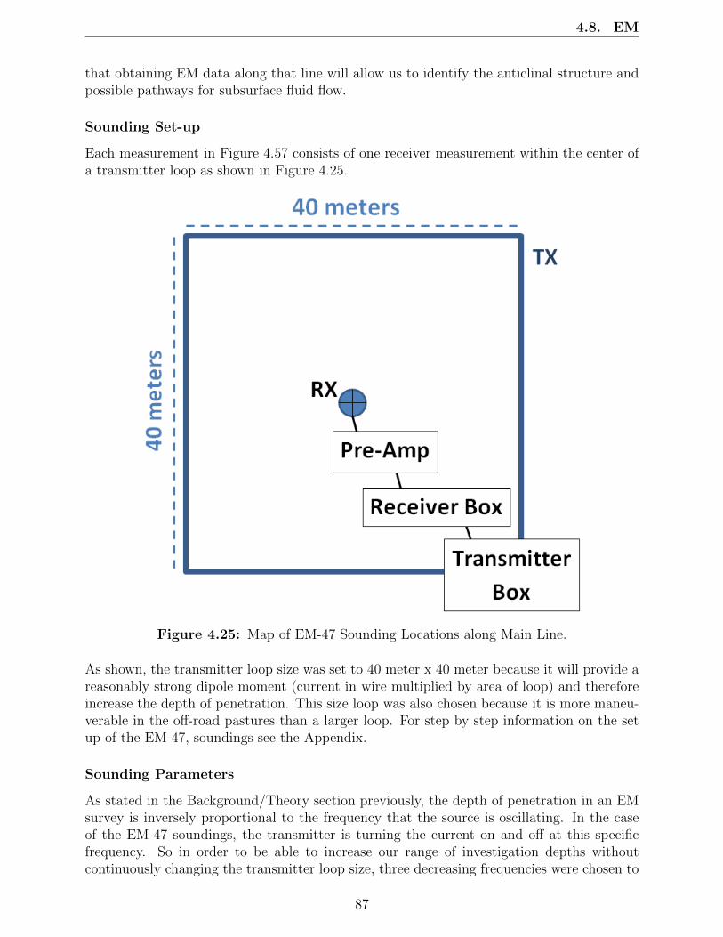
4.8. EM
that obtaining EM data along that line will allow us to identify the anticlinal structure andpossible pathways for subsurface fluid flow.
Sounding Set-up
Each measurement in Figure 4.57 consists of one receiver measurement within the center ofa transmitter loop as shown in Figure 4.25.
Figure 4.25: Map of EM-47 Sounding Locations along Main Line.
As shown, the transmitter loop size was set to 40 meter x 40 meter because it will provide areasonably strong dipole moment (current in wire multiplied by area of loop) and thereforeincrease the depth of penetration. This size loop was also chosen because it is more maneu-verable in the off-road pastures than a larger loop. For step by step information on the setup of the EM-47, soundings see the Appendix.
Sounding Parameters
As stated in the Background/Theory section previously, the depth of penetration in an EMsurvey is inversely proportional to the frequency that the source is oscillating. In the caseof the EM-47 soundings, the transmitter is turning the current on and off at this specificfrequency. So in order to be able to increase our range of investigation depths withoutcontinuously changing the transmitter loop size, three decreasing frequencies were chosen to
87

4.8. EM
perform measurements at (285Hz, 75Hz, and 30Hz respectively). The EM-47 receiver has thecapability to measure in X, Y, and Z components. However, measuring in more componentsrequires more time to perform measurements and it was decided measurements would onlybe made in the Z component so more stations could be completed along the line. Othernominal values such as current, integration time, and recordings per frequency were set aswell and can be found in the Appendix.
4.8.3 Processing
Data Conversion and Statistics
To begin processing, the raw data outputted by the EM-47 receiver was to converted fromgain scaled mV to nV/m2, which is units of magnetic flux. Along the Main Line there werethree recordings made for each frequency and these recordings were averaged and percenterrors were computed in order to obtain a representative sounding for each frequency at eachstation along the line. See the Appendix for the code used to convert and average the data.The decay of flux vs time was then plotted to preliminarily visualize the data, seen in Figure4.26. As seen with the jagged nature of the plot at later times, the data becomes noisy.Since later times respond to deeper depths of investigation, Figure 4.26 indicates that ourdata may not be able to fully resolve the resistivity structure at deeper depths.
Figure 4.26: Flux Decay vs Time from the data collected on May 18, 2014.
Apparent Resistivity
After the data was converted and averaged, it was processed using the plotting and inver-sion program IX1D. IX1D called for inputting the data in nV/m2 along with a timescale.This timescale is unique to each specific recording frequency with measurement intervalslocated logarithmically spaced on the receiver voltage decay curve (see Appendix for fre-quency timescales). IX1D also requires an associated error for each voltage measurement.Since the EM-47 does not record an error itself, the calculated percent error plus a baselineerror percentage of 5.0% was used for the Main Line data.
88

4.8. EM
The initial output from IXID consists of a Time vs Apparent Resistivity plot overlayingthe data collected from each frequency and current combination, as seen in Figure 4.27.
Figure 4.27: Apparent Resistivity Station 5.
Such plots were made for every station along the Main Line. Each square in the plotrepresents a voltage measurement converted into an apparent resistivity (see the Appendixfor this conversion formula). The three different colors correspond to the three differentfrequencies that were used at each station. The magenta is 285Hz, the royal blue is 75Hz,and the navy is 30Hz. By combining all of these plots and hanging them on a datumcorresponding to the linear projection of the Main Line, we were able to gain a first orderimpression of the resistivity structure within the subsurface.Figure 4.28 does not show the true underground resistivity structure, but it does give an im-pression of areas of interest within our section. Places where the apparent resistivity curvesdeflect from the vertical indicate depths that have changing resistivity; this could indicaterock type boundaries or other structures. From Figure 4.28, it appears that stations 31-27on the western side show relatively simple resistivity structures as those apparent resistivitycurves are simple. However stations 1-9 have more complex curves. This complexity becomessubdued moving farther east to stations 32-22.
89

4.8. EM
Figure 4.28: Section of apparent resistivity profiles along Main Line
By examining this plot we decided that inversions for true resistivity for depth would beperformed in areas of interest as indicated by the apparent resistivity curves such as be-tween stations 1-9.
90

4.8. EM
Inversion
From Figure 4.28, we chose to perform inversions on stations 31, 27, 26, 24, 1-6, 8,9, 32-37,and 10-22. Stations 32, 27, 26 and 24 were included for line completeness despite Figure4.28 indicating uninteresting structure. We did not invert the data from all sections due totime constraints.
In 1X1D, a one-dimensional (1D), four layer, half-space model was constructed and usedas a starting model for the station 31 inversion. The inversion results for this station wererefined until an acceptable percent RMS error existed between our modeled data and themeasured data (here, due to the noise in the data, acceptable RMS error values were 20%or lower). The inverse model for station 31 was then used as the starting model for thestation 27 inversion and so on, from west to east across the selected Main Line stations.This method for performing inversions was chosen as to attempt to laterally constrain eachinversion to be similar to the inversion preceding it to the east. A two-dimensional (2D) or,at least, pseudo-2D inversion would have been preferable but that was beyond the capabili-ties of IX1D.
Figure 4.29: Inversion model from station 5.
Figure 4.29 shows an example of an inversion performed on the data for station 5. Theright hand side of the plot shows the 1D layered model in red and on the left the smoothinverted apparent resistivity data is overlaid on the measured data shown as squares. Thegreen dotted lines on the layered model in Figure 4.29 correspond to models that are sta-tistically equivalent to the red model. The principle of equivalence in EM sounding is thatthe response from a thin layer is the same as a layer with twice the thickness but half theresistivity. The purpose of this equivalence test is to show that the inversion results are notunique, but at the same time some aspects of a model can be trusted as truer to reality ifthe difference between the equivalent model is small.
91

4.8. EM
2D Section
After all of the selected stations were inverted for 1D resistivity models, the data was thenexported and used to create a pseudo 2D section by stitching the 1D soundings together.
Figure 4.30: Psuedo-2D inversion from interpolated 1D sounding inversions
The code for plotting Figure 4.30 from the exported IX1D soundings can be found in theAppendix. In Figure 4.30, the data between each 1D inversion point, the black dots in thefigure, was interpolated using a cubic spline interpolation algorithm. Figure 4.30 has a loga-rithmic resistivity scale in Ω-m because our resistivity values range from less than 1 to over400.
As seen, there is very low data density within the plot and there is extensive interpola-tion and extrapolation. This was taken into account when interpreting the results.
4.8.4 Interpretation
Looking again at Figure 4.30, the depth scale extends to 250 meters below the surface. Asa general rule of thumb, the depth of induction by the transmitter loop in an EM-47 isproportional to roughly two to three times the transmitter side length. This gives us a depthof penetration of a maximum of about 120 meters. Recall that we also used multiple lowfrequencies to try to increase our depth of penetration; even so, it is obvious some of ourinversion data goes well beyond 120 meters. In fact, there are stations that were invertedfor depths over 400 meters. Also recall that depth of investigation is inversely proportionalto conductivity; therefore, a station over a more resistive area should image deeper than oneover a shallow area. By examining Figure 4.30, we see that stations 1-6 extend deeper thanstations 32-37 and are not consequentially located above a very resistive layer. By observingthe inversion data across all of the stations, we feel confident in our interpolation and averagedepth of investigation to plot at 250 meter depth.
However, Figure 4.30 does not give true representation of the subsurface. As stated be-fore, the data is heavily interpolated and many artifacts exist. For example, most of thesharp contours are a product of the lack of station density. Therefore, Figure4.30 must beregarded appropriately, but there are several structures that are worth noting. The mostobvious is the highly resistive shape between UTM 338500 and 339500. This shape beingcapture in seven inversions suggests that the shape is not an artifact but the expression of a
92

4.8. EM
true structure. Based on the knowledge of the Chromo Anticline and its geology, this couldbe interpreted as a resistive geological unit such as the Dakota Sandstone folded at the crestof the anticline. The resistive structure, in all likelihood, extends to the west but do to thelack of stations available in that area (Figure 4.57), that assessment cannot be corroboratedby data.
Moving further east along Figure 4.30 past UTM 339500 and station 9, there appears tobe a more conductive area. This may simply be the expression of shales underlying thesandstone beds that are now exposed due to erosion, or it could indicate the presence of afaulting structure filled with more conductive sediment or even fluids. This assessment seemsplausible because well logs that were investigated in the area tend to indicate the presenceof a fault. However, if there is a fault in the conductive region it must have considerablethrow because we do not see a matching resistive structure that could be the continuationof the Dakota Formation on the other side of the fault. Either it is a normal fault and theevidence is now eroded or a massive reverse fault that cannot be imaged by poor soundings.
Even further east of the conductive region, in Figure 4.30, lies a near-surface area of in-creased resistivity underlain by a significantly more conductive region at approximately 200meters depth. The near surface structure seen between station 32 and 22 does not have thesame resistivity values that the resistive body to the west has. In fact, they are significantlylower, on the order of 80 to 100 Ω-m. This indicates that the two resistive regions do notderive from the same rock unit. It can be seen that the resistivity of this structure is alsoincreasing along with depth to the far east in Figure 4.30. Based on this, as well as surfacegeologic information obtained in the area, it is proposed that this secondary resistive shapeis the Mesa Verde Formation dipping to the east on the east axis of the anticline. If thisstructure is the Mesa Verde then it is supporting the idea of the existence of a reverse faultand not a normal fault, which would cause the Mesa Verde to be eroded from our section.When looking at the depths of the inversion points between stations 32 and 22, the depth ofinvestigation does not go much beyond 200 meters. Therefore, the highly conductive regionseen at 200 meters depth is likely be being exaggerated by interpolation, but the data doesunequivocally indicate the presence of a more conductive region at that depth.
4.8.5 Sources of Error/Uncertainty
Electromagnetic methods are not very sensitive to physical noise such as wind, rain, orground motion; and since EM-47 is an active method, there are not errors introduced due tovariations in a natural field. However, EM methods are sensitive to cultural electromagneticnoise such as radio waves and power lines. Radio frequencies in the area are of low amplitudecompared to the field produced by our transmitter loop and do not introduce a significantamount of error into the data. However, along the Main Line there exists overhead powerlines over the entire profile. These lines are unshielded and are carrying significant current.The magnetic fields from these lines were undoubtedly detected by the EM-47 soundingsespecially were the power lines were in close proximity to the stations as with stations 32-37in Figure 4.57.
These sources of noise influence our data when the signal to noise ratio is low. Since theEM-47 measures the decay of the magnetic field produced by eddy currents in the Earth, at
93

4.8. EM
late times of observation the eddy currents are small and their corresponding magnetic fieldsare weak. These weak signals from the Earth are easily influenced by sources of error suchas the magnetic fields form the power lines. That is why the later time apparent resistivitiesin Figure 4.28 become noisier. This noise affects how we were able to perform inversions onour data; noisy data makes our inversions more non-unique and also prevents our modelsfrom producing data that fits our measurements well. This higher amount of noise seen atgreater depths reduced our confidence in the interpretation of deeper features in Figure 4.30.
4.8.6 Conclusion
We believe the goal of mapping the subsurface resistivity structure along the Main Line wasmet by the collection of EM-47 soundings. Through various data manipulations, a set of 1Dsounding inversions were obtained and then compiled into a psuedo-2D section parallel tothe Main Line.
Figure 4.31: Psuedo-2D inversion from interpolated 1D sounding inversions
We have discussed multiple possibilities for the resistivity structures seen in Figure 4.30 andhave concluded on the final interpretation seen in Figure 4.31. This interpretation showsthe Dakota Sandstone entering from the west into the Chromo Anticline and then beinginterrupted by a large reverse fault leaving the Dakota far below in the eastern portionof the section. In the near surface on the east, we have interpreted that the resistive bodypresent is the dipping Mesaverde Formation. Areas indicated by a question mark do not haveenough information or are interpolated extensively and no confident interpretation could bemade. To be sure, this is an interpretation only from what we have observed in the field andthe resistivity structure seen from our interpolated 1D sounding inversions. Combining thisdata with another relatively shallow dataset would be able to illuminate areas of uncertainty.
94

4.9. Magnetotellurics
4.9 Magnetotellurics
4.9.1 Survey Location
The magnetotelluric survey location was spaced out along the Main Line on County Road382. During our seven days of acquisition we completed ten sites total. These sites coveredapproximately nine kilometers which gave us an approximate 2D pseudo section along theMain Line. Because we had limited access to property along the Main Line, the station spac-ing was not even forcing us to interpolate between these areas with higher station spacing.Ten surveys were conducted north of CR382 and two sites were conducted south of the MainLine. Specific locations for the twelve MT sites can be seen in Figure 5.1.
Figure 4.32: MT site locations on Main Line.
4.9.2 Survey Design
All of the magnetotelluric sites were acquired in open fields in order to space the electrodes100.0 meters apart. This spacing was used for all the sites except for site 11 where an80.0 meter grid had to be used due to a nearby river. Figure 4.33 shows the electrodesspaced 50.0 meter from the orange ADU-07 box out in both the Ex and Ey directions. TheHx and Hy magnetometers are typically 5.0 m to 10.0 meter away from the ADU-07 andbattery in order to reduce noise. One magnetometer was lined up facing north and theother facing east. In order to reduce temperature variations throughout the data collection,both magnetometers were buried approximately one to two feet deep. Figure 4.33 showsa Hz, or vertical component, magnetometer which was not used in our data acquisition.The electrodes were lined up north to south and east to west. Electrodes were also buriedapproximately one foot in the ground and attached to the ADU by cables to increase the
95
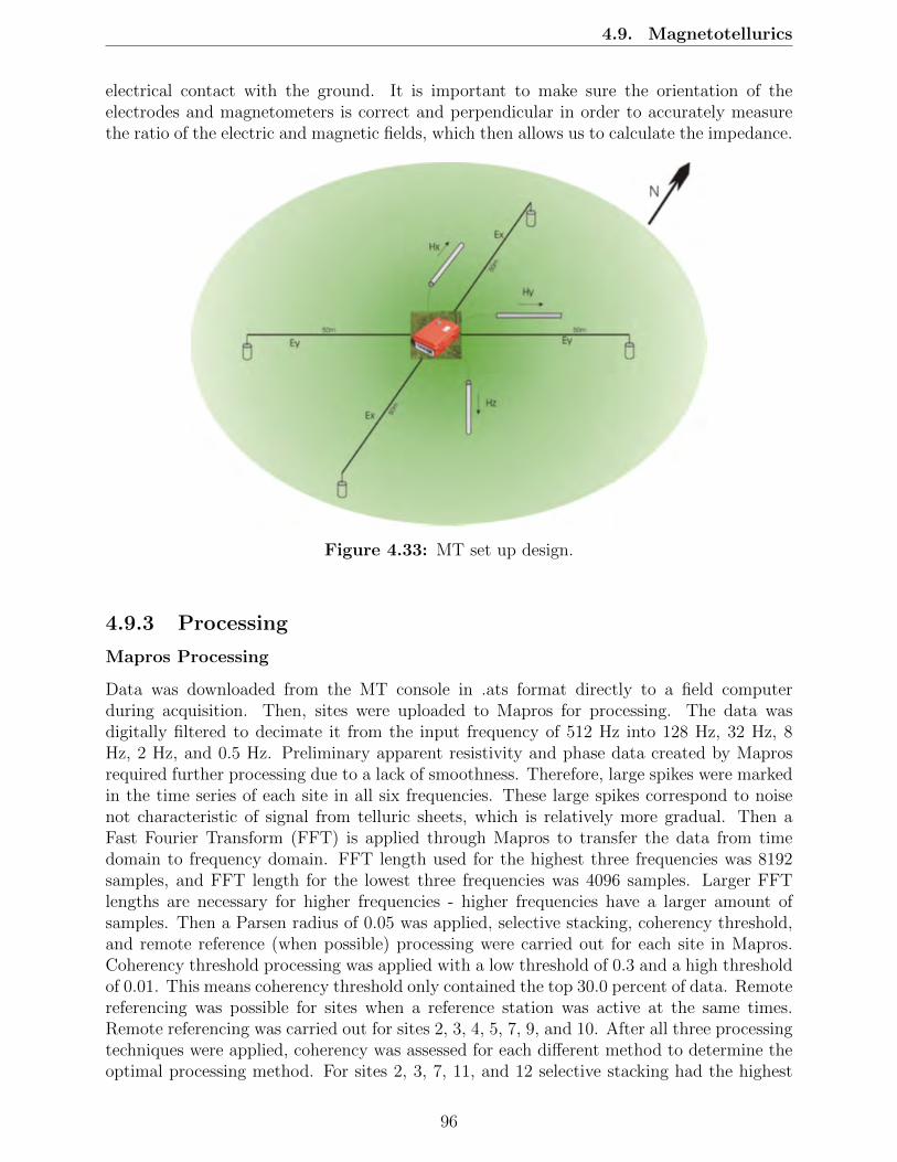
4.9. Magnetotellurics
electrical contact with the ground. It is important to make sure the orientation of theelectrodes and magnetometers is correct and perpendicular in order to accurately measurethe ratio of the electric and magnetic fields, which then allows us to calculate the impedance.
Figure 4.33: MT set up design.
4.9.3 Processing
Mapros Processing
Data was downloaded from the MT console in .ats format directly to a field computerduring acquisition. Then, sites were uploaded to Mapros for processing. The data wasdigitally filtered to decimate it from the input frequency of 512 Hz into 128 Hz, 32 Hz, 8Hz, 2 Hz, and 0.5 Hz. Preliminary apparent resistivity and phase data created by Maprosrequired further processing due to a lack of smoothness. Therefore, large spikes were markedin the time series of each site in all six frequencies. These large spikes correspond to noisenot characteristic of signal from telluric sheets, which is relatively more gradual. Then aFast Fourier Transform (FFT) is applied through Mapros to transfer the data from timedomain to frequency domain. FFT length used for the highest three frequencies was 8192samples, and FFT length for the lowest three frequencies was 4096 samples. Larger FFTlengths are necessary for higher frequencies - higher frequencies have a larger amount ofsamples. Then a Parsen radius of 0.05 was applied, selective stacking, coherency threshold,and remote reference (when possible) processing were carried out for each site in Mapros.Coherency threshold processing was applied with a low threshold of 0.3 and a high thresholdof 0.01. This means coherency threshold only contained the top 30.0 percent of data. Remotereferencing was possible for sites when a reference station was active at the same times.Remote referencing was carried out for sites 2, 3, 4, 5, 7, 9, and 10. After all three processingtechniques were applied, coherency was assessed for each different method to determine theoptimal processing method. For sites 2, 3, 7, 11, and 12 selective stacking had the highest
96

4.9. Magnetotellurics
coherency, and coherency threshold processing yielded the highest coherency for sites 1, 4,5, 9, and 10. Sites 6 and 8 were solely reference stations and required no further processing.A coherency plot generated from site 7 can be seen in Figure 4.34.
Figure 4.34: Coherency plot of site 7. The X-axis represents frequency and the Y-axisrepresents coherency.
Excel Processing
Data was then exported in ASCII format with the optimal processing technique applied,downloaded, and compiled in Excel. Apparent resistivity vs frequency plots were made inthe XY and YX direction for each site in order to determine if any sites needed to be rejected.Ideally, the apparent resistivity should be as smooth as possible and following a similar trendfrom west to east. It was determined that site 9 would be rejected due to cows chewing onthe cable causing only thirty minutes of usable data. Each frequency had one to threecorresponding resistivity and phase values. In order to input the resistivity and phase intothe inversion program IPI2win, these values had to be weighed over each frequency. Thiswas programmed into excel using Equation 4.5, where xi is the resistivity or phase value fora specific frequency and σ2 is the variance given in the ASCII file. This produced a singleresistivity and phase value in both the XY and YX directions over every frequency for eachsite. The accuracy of each resistivity and phase value was also calculated. First, the averagevariance was calculated for each point and then normalized using Equation 4.6. These valueswere then subtracted from one in order to obtain the accuracy of each point. The frequency,resistivity, phase, accuracies, and horizontal location of each station was then importedinto IPI2win for interpretation. Additionally, the signal coherency was assessed in the XYand YX polarizations before producing inverted models. Signal in the YX polarization hadconsistently low coherency across the frequency range sampled, and was therefore not usedto produce resistivity models.
97

4.9. Magnetotellurics
x =
∑xiσ2∑1σ2
(4.5)
Xi =Xi −min(X)
max(X)−min(X)(4.6)
Inversion
Apparent resistivity, phase, and accuracy estimates were used to produce a true resistivitymodel with IPI2win. Multiple inversion techniques were applied to find an optimal solution.A 2D pseudo section was created from an inverted two layer model, and Occam’s Inversionalong with a 4 layer model inversion were carried out. Resolution was maximized withOccam’s Inversion, as a fine discretization was carried out and data misfit and smoothnesswere optimized. The simple 2 layer model provides a useful first order pseudo section forinterpretation. After inverting models with multiple inversion techniques, models with thelowest root mean square (RMS) error were selected. Models with RMS error significantlyover 50% were eliminated from the integrated model, but still used in the MT pseudo sectionand interpretation. Sites 4 and 5 were used in the integrated interpretation and may be foundin the integrated section accordingly. These sites had the lowest RMS values - sites 4 and 5had RMS values of 22% and 24% accordingly.
4.9.4 Interpretation
The data was inverted using IPI2win, which created a 2D pseudo section of the Main Lineand resistivity and phase curves for each of the sites. In order to create the inverted image,we used a simple two layer model over a halfspace (Figure 4.35). In this case, we mod-eled the sandstone and shale over the Precambrian basement. This allowed us to analyzethe data in order to determine if there were any further sites that needed to be rejectedfrom the final image. After importing the YX data into the program we observed that dueto the magnetometers being orthogonal with the nearby power lines there was an abundantamount of noise and artifacts in the pseudo section which caused the data set to be unusable.
The pseudo section produced by the XY data over sites 2, 4, 7, 10, and 11 was noticeablyless noisy and is seen in Figure 4.36. Here, the red arrows represents where our sites werelocated with an interpolation between the sites. In this pseudo section we can see a generaltrend of conductivity increasing as we go east at all depths. A highly resistive body startingaround one kilometer primarily on the eastern side is also visible. We believe this is becausethe highly resistive basement rock is significantly closer to the surface in this area due to apossible thrust fault. We can also see how the basement rock is closer to the surface due tothe anticline structure, which is confirmed in this model. Figure 4.36 represents the apparentresistivity and phase curves with added error bars which helped smooth the inversion fromartifacts. Here we can also calculate a rough estimate of the resistivity of the basement rockranging from 1000-10000 Ωm.
If we look at a shallower depth pseudo section, as shown in Figure 4.38, we can see a strongcontrast going from resistive to conductive. This pseudo section was also transformed toa linear scale instead of a log scale used in the previous image. This further supports our
98

4.9. Magnetotellurics
Figure 4.35: Resistivity and phase curves modeled as 2 layers overlying a halfspace. Ap-parent resistivity is the top plot while phase is below.
Figure 4.36: Pseudo section covering the Main Line where we can see a conductive toplayer and resistive bottom layer on the west side.
hypothesis that there is a potential thrust fault which caused the sediments on the footwallor eastern side to remain uneroded giving us a higher conductivity.Our next interpretation was centered around the crest of the anticline focusing on sites 2, 4,and 5. The purpose was to create a model that better fitted with the geology and increasedresolution using data given from other geophysical methods. In the Occam’s inversion tech-nique applied, a much finer discretization interval is made and data misfit is minimizedand smoothness is maximized. Figure 4.39 shows the interface between the basement and
99

4.9. Magnetotellurics
Figure 4.37: Resistivity and phase curves modeled as 2 layers. Error bars represent accu-racy of data.
overlying rocks at approximately 1.5 kilometers on the right of the fault. The fault washypothesized to be a reverse fault due to the angle and amount of offset. We can also see aresistivity of approximately 50,000-60,000 Ω*m of the Precambrian basement. Conductiveanomalies are observed above site 4 and 2. These may relate to relative increases in poros-ity, permeability, moisture content, temperature, or clay content. No clear trends in layerswithin the sedimentary package above the basement are observed. This could result froma lack of resistivity contrasts on a scale comparable to the vertical resolution of the MTsoundings or from Galvanic distortion. Data misfit was calculated for the Occam’s inversionin order to assess the accuracy of the data. Sites 5 and 2 had the lowest data misfit, withroot mean square error values of 23.2% and 19.34% respectively. Site 4 had the highest rootmean square error value at 54.4%. The degree of error between the calculated data from theinverted model and the observed data warrants the integration of other geophysical methodsor further MT surveying in order to make an accurate geological interpretation.
100

4.9. Magnetotellurics
Figure 4.38: Close up image of pseudo section over anticline with a linear scale.
Figure 4.39: Geoelectrical section of sites 2, 4, and 5 centered around the anticline.
4.9.5 Sources of Error/Uncertainty
Error
Any local sources of electromagnetic waves create EM fields that violate the plane waveassumptions necessary for MT surveying. One of the largest sources of error in MT is thenoise created by power lines. Ideally, MT surveys should be performed at least a kilometeraway from any power lines or other metallic human made objects, such as metal fences. The
101

4.9. Magnetotellurics
survey locations contained multiple power lines that were often within meters of the grid.Since there were multiple houses along the Main Line, this also created a large amount ofnoise in the data. The surveys ran at night to decrease the noise caused by human activity.Still, cars are likely to have driven by the MT station during acquisition, which would causenoise in the readings through the physical perturbations of the sensors and the EM sourcefields produced by the cars. Cattle caused error by chewing on cables and causing them toget unplugged, disoriented, or displaced. Site 9 MT station cables were chewed by cattle,and site 9 data was incoherent and not used accordingly.
Uncertainty
Another possible source of uncertainty includes magnetometers or electrodes not beingplugged into the correct location corresponding to the direction on the ADU. This shouldbe able to be detected during processing when looking at the raw data for the electric andmagnetic fields and if needed can be switched in Mapros. Correlation between orthogonalelectric and magnetic channel indicates the channels were connected correctly. Clear corre-lation between two parallel electric and magnetic fields was detected during processing andthe channels were changed accordingly, but detecting the correlation between channels wasgaugued subjectively and error was possible. Additionally, the quality of signal varies byfrequency, and some bands contain little to no usable signal. Coherency plots (Figure 4.40)are used to assess the quality of the data in the frequency domain and can be found in theAppendix for Sites 1, 7, and 12. Low coherency was observed in data corresponding to the0.1 Hz to 4 Hz frequency range[43]. This dead band of low quality data is characteristic offrequencies where signal to noise ratio is poor, and the coherency of the data was accountedfor during interpretation. The depths of the dead band were found by matching the frequencyrange with the inverted model, and dead band depths are between 1.6 km and 15 km[43].Galvanic distortion also produces noise in the data. As sounding period increases and theinductive scale length, or electromagnetic skin depth (see Appendix), becomes significantlygreater than the scale of anomalous bodies, a non-inductive response from the anomalousbody persists[43]. This is equivalent to a static shift effect within the data.
102

4.9. Magnetotellurics
Figure 4.40: Coherency plot with a noticeable dead band around 1 Hz.
4.9.6 Conclusion
MT is a passive experiment using natural sources with a high depth of penetration comparedto other geophysical methods used in this study. MT allows us to compare the orthogonalmagnetic and electric fields which enables us to calculate the apparent resistivity of the sub-surface. The data was processed in order to decrease noise and artifacts in the inversion andthen interpreted using the known geology of the area. Due to a large amount of noise presentand low resolution images we were unable to determine any geological structures withoutdata from other surveys. However, we were able to locate a conductive top layer overlayinga more resistive basement. We were able to make a preliminary geological interpretation butintegration with other methods is necessary to interpret the subsurface with greater con-fidence. The pseudo section created helped support previous known information and datacollected from other surveys in this study. If future investigation is performed, it would berecommended to use a site at least one kilometer away from all utility lines to decrease thenoise present in the data.
103

4.10. Ground Penetrating Radar
4.10 Ground Penetrating Radar
4.10.1 Survey Location
The GPR survey along the Main Line extended from the west end of the Main Line to theeast end, along County Road 382. Exact locations were determined by differential GPS,which was recorded at each flag location along the Main Line. The total length of the GPRsurvey was 9.0 kilometers.
Figure 4.41: Main Line GPR Survey Location
4.10.2 Survey Design
Antenna separation was kept constant for a fixed or constant offset profiling. A 1000 MHzsystem and a 500 MHz system were both considered for use at this field site. We decidedto use the 500 MHz system so that we could see slightly deeper than the 1000 MHz system(as lower frequency corresponds to deeper penetration). It was determined that with thisantenna resolution was still high enough to locate shallow anomalies. Our target anoma-lies consisted mostly of wires and cables running beneath the road. The Main Line flags,located every 10 meters, were marked and measured on the GPR using the fiducial buttonand distance was tracked using the attachable wheel as an odometer. To acquire data, theGPR user must walk slowly backwards while dragging the GPR system. Instantaneously,the visual monitor displays the data.
104

4.10. Ground Penetrating Radar
Continuous data was taken every .025 seconds along the Main Line. Each section of data is20 meters in length with an additional meter for overlap at each end.
4.10.3 Processing
Our GPR data was processed using the program Ekko View 2. GPR data closely resemblesseismic data, therefore, we used similar processing techniques. With time, our signal ampli-tude begins to decrease because the energy diffuses as it travels farther through the ground.Because of this, we apply an automatic gain control (AGC) to smooth out the data. We alsoapply color contrast between the lines so that anomalies will stand out more. If we noticea distinct hyperbola, then we could apply more filters to the line to adjust the time scalein order to fit the data better. We were able to accurately identify what was making theanomalies in the data with correlation with the field notes. Most of the anomalies that wereseen on the GPR data were a result of buried cables, culverts, geophone cables, or surfacenoise. Once we identified the sources of the different anomalies, we were able to map wherecables and culverts are located along the Main Line.
4.10.4 Interpretation
The first thing that we should note from the GPR images, is that the x-axis is mislabeled.The GPR uses an odometer in the back wheel that keeps track of how far it is traveling.Each of the flags had 10.0 meter spacings and each line measured a length of 2 flags, or20.0 meters. Each of the measurements show that the GPR only traveled about 15.0 metersbetween two flags, so the odometer and GPR were not calibrated correctly. However, aftercompiling the lines, we were still able to identify all of the potential anomalies. We can seein Figure 4.48 and Figure 4.44 that the main anomalies are due to buried cables and culvertsin the area. These anomalies appear as hyperbolas on the line. Figure 4.47 shows unwantednoise in the data. In Figure 4.47, we can see an apparent anomaly that was actually gener-ated from the GPR instrument running over a loose geophone cable on the ground. This willproduce vertically noisy data over the extent of the line. Additionally, within many images,multiples can be seen. The multiples can clearly be seen in Figure 4.47 at a depth of 1.4meters to 1.8 meters.
Once the anomalies were identified with the GPR data, we were able to create a map ofthe anomalies and identify what source was buried at that location. However, not all of theanomalies that we expected to find were located with the GPR survey. There were manyculverts and cables that we visually identified that were not detected by the GPR. This couldhappen if the features are buried deeper than the GPR can image. In Figure 4.49, all of thecultural features and visually identified features are shown.
4.10.5 Sources of Error/Uncertainty
The main source of error in a GPR survey is poor contact with the ground. Poor contactwith the ground can be the result of rough terrain, large rocks, or other obstructions onthe surface, such as geophone cables. When the GPR instrument is lifted off the ground, itcauses a loss of electromagnetic energy into the air instead of propagating the full amount
105

4.10. Ground Penetrating Radar
Figure 4.42: Line taken at Main Line flag 1134. We can see that the anomaly shown at9.25 meters comes from running over some geophones cables with the GPR.
Figure 4.43: Line taken at Main Line flag 1080. The anomaly shown at 0.75 meters ismade from a buried power cable.
Figure 4.44: Line taken at Main Line flag 1012. This shows the culvert that was locatedat the 8.75 meter mark.
of energy into the ground.
Sources of error due to processing consist of potentially choosing incorrect parameters whenvisually selecting parabolas and anomalies of importance within EKKO View.
While processing data, we also discovered discrepancies in notes that led to 2.2 kilome-ters of missing data between flags 1346 and 1752 along the Main Line. Luckily, GPR is notan integral part in combining the various other geophysical methods for an overall interpre-tation.
106

4.10. Ground Penetrating Radar
Figure 4.45: Cultural features that were visually identified and that were detected by theGPR.
4.10.6 Conclusion
Overall, the processed GPR data can be used as confirmation of near surface cables andother anomalies that could potentially cause noise for the other methods within the surveyalong the Main Line. The data could also be used to formulate shallow velocity modelsto help in the processing of other data. Generally, GPR data behaved as expected. Themajority of marked cables were apparent along the Main Line, however some were buriedtoo deep or did not produce a strong enough signal to be seen using the 500MHz system.
107

4.11. Hammer Seismic
4.11 Hammer Seismic
4.11.1 Survey Location
The field site locations for hammer seismic were chosen based upon inferred geologic struc-tures and known surface features. The hammer seismic line along the Main Line was locatedbetween flags 1281 and 1291, just past the Stinking Springs. The line was not centered atthe springs due to geometric complications and was instead situated on the nearest straightstretch of County Road 382, to the north of Stinking Springs.
Figure 4.46: Hammer seismic survey location along the Main Line.
4-H Site at Pagosa Springs
One line was taken in the 4-H Club parking lot for students who had not previously acquiredhammer seismic data at the Main Line or Student Site. This line was set up as a demon-stration for high school students, not as a source of subsurface data acquisition for the mainproject. Analysis done on this data was solely for quality control and has been included forframe of reference.
4.11.2 Survey Design
Each line consists of a cable attached to 48 geophones. For the P-wave surveys, verticalcomponent geophones were used with a vertical impact source; for the S-wave surveys, hor-izontal component geophones were used and the source data was collected from both sidesof the line. For every 24 geophones, there is a seismograph that converts the analog signal
108
4.11. Hammer Seismic
running through the cable from each geophone into a digital signal that is sent back to alaptop.
For the main line, spacing between geophones was 2.0 meters for both P-wave and S-wave,making the length of these lines 96.0 meters. Seismographs were situated at 48.0 meters and96.0 meters on the line and data acquisition began at 97.0 meters. There were 10 stackstaken for each p-wave shot located between every eighth geophone (16.0 meter spacing). Forthe S-wave data, there were three stacks taken on both face plates of the S-wave shot atthree locations: 96.0 meters, 48.0 meters, and 0.0 meters.
4.11.3 Processing
To process the hammer seismic data, we worked with Seismic Unix (SU). Because the datathat we gathered in the field was in SEGY format, we first had to convert it to a .su file.Once it was converted, we had to change the headers of each file to fix the geometries foreach shot of the line. We then had to adjust the locations of each shot and how they werespaced. Some files had compressed each of the shots into one shot, so we had to split thesefiles up into all of the various individual shots.
Once our files and geometries were all fixed, we were able to look at all of the shots in-dividually and create images of them using SU. To produce all of the images, we had to usethe terminal on a Unix computer and communicate using SU commands. Our main goal isto produce a shot image clear enough to measure the different layer velocities of both thedirect wave and the head wave.
The processing for the Main Line and the Student Site hammer seismic data was identi-cal. We will use Shot 3008 as an example to show how we created the images. This shot islocated on the 145.5 meter mark of the Student Site line. We first made a simple gray-scaleimage of the shots, as shown in Figure 4.47. However, this image is low resolution, so weadded gain to the image, which produced the image in Figure 4.48. In this figure, we cansee higher resolution, but not high enough resolution to accurately estimate slope velocities.In order to better see the refractions in the shot gathers, we added a function that took onepercent of the outliers and normalized them to match with the rest of the data. The imageproduced by using this function can be seen in Figure 4.49. Now we are able to more clearlysee where the direct wave and the head wave might be. In order to get a closer look at thewaves we are particularly interested in, we reduced the window size up to 0.1 seconds toeliminate extraneous information. To get rid of some of the other unwanted noise, we alsoapplied a band pass filter using the frequencies 30Hz, 40Hz, 100Hz, and 120Hz. This createdFigure 4.50 which is resolved enough to determine the different velocities of the subsurfacelayers. Using the same parameters, we can also create a wiggle plot, as shown in Figure4.51. This wiggle plot can be used as a reference to make sure that we can correctly identifythe head wave and the direct wave. It is also helpful because it shows the lines that eachgeophone is measuring. This process was repeated for every significant shot gather located atthe beginning, middle, and ends of each hammer seismic line for comparison and consistency.
Now that we have a clearer image, we can manually calculate our velocities by lookingat the sharper refraction lines created through processing. To do this, we hand drew a line
109

4.11. Hammer Seismic
from the surface where the shot was taken that follows the direct wave and a second thatfollows the head wave, as shown in Figure 4.52. We are able to calculate the velocities usingthe slope of these lines. The slope drawn using the direct wave will let us know the velocityin the first layer and the slope of the head wave will tell us the faster velocity of the secondlayer. We also need to find the time that the head wave line crosses the offset line in order tocalculate a depth of the top of the second layer. This is easy, as the vertical axis is alreadymeasured in time. With this information, we can use Equation 5.2 to calculate the depth.We can repeat this process with different shots along the line to check if the layers are vary-ing or dipping. If we do notice that the layers are not horizontal, we can use Equation 5.8to calculate the dip of the layer. Knowing the different depths and dips of the second layerhelps to create a simple geologic model of the subsurface.
Figure 4.47: Example of a grayscale image made using Shot 3008
110

4.11. Hammer Seismic
Figure 4.48: Example of gain applied to Shot 3008
Figure 4.49: Example of smoothing function applied to Shot 3008
111

4.11. Hammer Seismic
Figure 4.50: Example of Shot 3008 with an adjusted window size and a band pass filter
Figure 4.51: Wiggle plot of Shot 3008 with the polarity reversed to more accurately identifythe first arrival.
112

4.11. Hammer Seismic
Figure 4.52: Example of how we calculate the velocities of the head wave and the directwave on Shot 1009
4.11.4 Interpretation
The 4-H model shown in Figure 4.53 demonstrates the simplest of two layer systems in whichthere was no true dip found on the line of geophones. This location was used as a learningaid for both processing and calculations to be applied to the more complicated Main Lineand Student Site.
The simple 2-D sections have been created based upon results found from processing variousshots and then finding depth and dip using calculations previously discussed. The MainLine image shown in Figure 4.54 depicts a two layer model, with Layer 1 having a thicknessof approximately 5.0 meters and Layer 2 is shown as a half space due to depth limitations.We have calculated the dip to be approximately 3 degrees which could be caused by thehammer seismic line location in relation to the hinge axis of the Archuleta Anticline. Therewas a flatter refraction towards the west end of the line which translates to a faster velocity.This has been interpreted to potentially be a fault, however our line of data only barelyoverlapped this anomaly. Upon comparing the data to that of deep seismic, it appears asthough their final post stack depth migration also reflects a fault in this same location.Hammer seismic refraction interpretation consists of these following steps.
1. Choosing the refraction method.To begin with the refraction analysis, we have to choose the reflection method that fitwith the local geological setting in the area. Three common methods are (1) a singlesubsurface interface, (2) two horizontal interfaces, and (3) dipping interfaces.
113
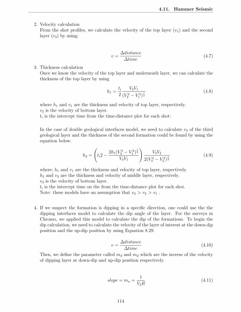
4.11. Hammer Seismic
2. Velocity calculationFrom the shot profiles, we calculate the velocity of the top layer (v1) and the secondlayer (v2) by using:
v =∆distance
∆time(4.7)
3. Thickness calculationOnce we know the velocity of the top layer and underneath layer, we can calculate thethickness of the top layer by using
h1 =ti2
V2V1
(V 22 − V 2
1 )12
(4.8)
where h1 and v1 are the thickness and velocity of top layer, respectively.v2 is the velocity of bottom layer.ti is the intercept time from the time-distance plot for each shot:
In the case of double geological interfaces model, we need to calculate v3 of the thirdgeological layer and the thickness of the second formation could be found by using theequation below.
h2 =
(ti2−
2h1(V23 − V 2
1 )12
V3V1
)V3V2
2(V 23 − V 2
2 )12
(4.9)
where; h1 and v1 are the thickness and velocity of top layer, respectively.h2 and v2 are the thickness and velocity of middle layer, respectively.v3 is the velocity of bottom layer.ti is the intercept time on the from the time-distance plot for each shot.Note: these models have an assumption that v3 > v2 > v1 .
4. If we suspect the formation is dipping in a specific direction, one could use the thedipping interfaces model to calculate the dip angle of the layer. For the surveys inChromo, we applied this model to calculate the dip of the formations. To begin thedip calculation, we need to calculate the velocity of the layer of interest at the down-dipposition and the up-dip position by using Equation 8.29.
v =∆distance
∆time(4.10)
Then, we define the parameter called md and md which are the inverse of the velocityof dipping layer at down-dip and up-dip position respectively.
slope = mu =1
V2R(4.11)
114

4.11. Hammer Seismic
slope = md =1
V2F(4.12)
After that, we use these two following equations to figure out the dip of interestedsubsurface layer.
θic =arcsin (V1md) + arcsin (V1mu)
2(4.13)
β =arcsin (V1mu)− arcsin (V1md)
2(4.14)
Detailed explanation on each variable and model could be found in the hammer seismictheory and background section.
Figure 4.53: 4-H hammer seismic site 2 layer model.
115

4.11. Hammer Seismic
Figure 4.54: Main Line hammer seismic 2 layer model.
4.11.5 Sources of Error/Uncertainty
Hammer Seismic has many sources of error and uncertainty. There are errors in ac-quisition from inconsistent hammer strikes across a stack of shots, not flipping thepolarity of an inverse shear shot, reversing s-wave geophones, missing the plate witha strike, using faulty equipment, and from noise from walking people, cars, burrowinganimals etc. For inconsistent strikes the amplitudes could shift when they are stacked.For shear shots, we first strike perpendicular to the line in one direction and then theother as shown in Figure 4.55 and Figure 4.56. This causes responses with oppositeamplitudes, which causes destructive wave patterns. There are errors in processingcaused by applying improper filtering that removes the first arrival, drawing improperlines for the direct and head wave, having shot locations in the wrong area relative tothe whole line, having shots mislabeled, and entering data wrong.
116

4.11. Hammer Seismic
Figure 4.55: North facing shear strike.
Figure 4.56: South facing shear strike.
117

4.11. Hammer Seismic
4.11.6 Conclusion
Hammer seismic data along the Main Line concurs with the shallowest part of deepseismic data. As this line was taken just east of Stinking Springs and the ArchuletaAnticline was found to peak farther east, the slight dip west makes sense geologically.There also appears to be a fault at the west end of the hammer seismic line that alignswith fault imaged in the deep seismic stack. Both of these points demonstrate theefficacy of utilizing hammer seismic data in the interpretation of geology along thisportion of the Main Line.
118

4.12. Deep Seismic
4.12 Deep Seismic
Deep seismic methods commonly used in geophysical interpretation because high qualityseismic data can give images with depths over 5000 meters. However, there are drawbacksto using this method such as the time, energy and expense that goes into a seismic surveyand the fact that the resolution is not as good as shallow seismic methods such as HammerSeismic. However, certain techniques in survey design, acquisition and processing can givea better resolution to the data. Survey design is a very important part in seismic datainterpretation, and is often times the first step in the seismic method. It is important todesign a survey and use survey parameters that will aid in achieving the highest possibledata resolution, while maintaining the desired depths in order to image the targeted geologicstructures.
4.12.1 Survey Location
The seismic line was determined based on the geology in the area, and accessibility thatthe vibrator trucks had to the area. County Road 382 outside of Chromo runs across theanticline in a diagonal relation to the axis of the anticline. This can be seen in Figure 4.57below. The main seismic line where data was collected was set up along the north side ofCountry Road 382. This allowed for easy accessibility for the vibrator trucks while still beingable to go over the axis of the anticline to get an accurate image of the geologic layers thatexist. This is important to aid in other method’s interpretation of physical rock properties.
Figure 4.57: Map of Survey Location in relation to the anticline axis
119

4.12. Deep Seismic
4.12.2 Survey Design
In order to get a good understanding of the geology and what exists beneath the surfacewhen using the seismic method, it is very important to design a survey that will give you theinformation you are looking for. Considerations need to be made about the topography ofthe area and if a grid can be set up over the area. Areas that have steep topography and orhave water features such as rivers and streams are much more difficult to acquire data overthan areas that are flat. Considerations also need to be made on what exactly the problembeing investigated is and what the purpose of the seismic survey is. Our purpose in Chromowas to understand where the water is coming from, how the geothermal system in the areaworks and if it is connected to the Geothermal system in Pagosa. We needed a survey thatwould have good resolution at shallow depths so that faults and fractures could be imaged.This guided our decision making process regarding the selection of survey paramters.
Survey Parameters
There are many different parameters that need to taken into consideration when designinga seismic survey such as how the spread will be set up and what the sweep parameters willbe. The spread consists of where the sources and the receivers will be set up, and what thedistance between each station will be. The survey design will also determine whether thesurvey will be an off-end verses a split spread survey. We decided that the seismic surveywould consist of a source station spacing of every ten meters, with receiver station spacingof every ten meters, using a split spread survey. See the Appendix for a more detailed de-scription of how a split spread seismic survey is set up. Our spread was an off end spreaduntil we collected data for 120 channels, and then it changed to a split spread survey untilit reached the end.
Another important aspect of creating an accurate seismic survey that will produce gooddata is to have a good seismic source. There are several different methods of creating a seis-mic source and each method has its advantages and disadvantages. Our survey conducteddown in the Chromo valley used a vibrator source which is a source that sends energy intothe ground using a large vibrator truck. The energy is produced by vibrating a weight on apad that is held in contact with the ground, so the vibration is propagated into the earth. Avibrator will go through a sweep which is a set of parameters that determines the frequenciesand the period of time that the plate vibrates on the ground at each source station. Multiplesweeps are often times done at each station.
Sweep Parameters
Another set of parameters that needs to be considered when designing a seismic survey aresweep parameters. Sweep parameters consist of how long and at what frequencies the platewill shake at, and how many times the plate will shake at each station, which is also known asthe number of sweeps. Sweep parameters are determined by conducting sweep tests. Sweeptests are conducted before data acquisition begins to make sure that the ground responsefrom the vibration parameters produces a good signal. Different parameters can give dif-ferent results and the parameters chosen are based off of knowledge of the geology in the area.
The sweep parameters that were used for this survey are the desirable set of parameters
120

4.12. Deep Seismic
to use for an area that has shallow geology. The parameters used for this survey were de-termined after doing of three different test which resulted in a linear sweep going from lowfrequency to high frequency. Frequencies of each sweep ranged from 6 Hz to 180 Hz andincreased over a 14 second time period. Data was recorded from the geophones for a totalof 22 seconds, this included a 14 second sweep time plus a four second listen time. Thefour second listen time was to ensure that the signal was reflected off of the deepest layersand returned to the receivers. Four sweeps were done at each source location and this wasto help improve the signal to noise ratio (See Fold Appendix). The number of sweeps willdetermine the fold of the survey. The higher the fold, the better the resolution of your datawill be. However, doing too many sweeps at each station can be costly and time consuming,and so a number is needed that is a balance of time available and data quality.
121

4.12. Deep Seismic
4.12.3 Processing
Figure 4.58: Overview of the data processing for seismic used in this study
122

4.12. Deep Seismic
Geometry
In order to account for the geometric layout of the survey, the GPS survey informationcontaining the X, Y and elevation coordinates and observer notes from acquisition wereimplemented into the data. For each shot and receiver a coordinate was assigned and usedto create a spatial distribution of the midpoints on a UTM grid (Figure 4.59). As the surveyline, and subsequently the distribution of midpoints, did not follow a spatially linear trend,it was important to assume a crooked line geometry. In order to account for the irregularity,we utilized three best fit line segments effectively binning the midpoints to create a collective2D line. Geometry becomes particularly important when considering the concept of fold, orsignal-to-noise ratio, which increases toward the center of the line (Figure 4.60). With thecontinuation of processing on this section, the fold is an implied constraint on the quality ofthe data, ultimately effecting the quality of the final deliverable image ( See Fold Appendix).
Figure 4.59: Map view of entire seismic line running from East to West along CR-382. Linesits on the distribution of midpoints(white) and provides an elevation scale(blue = 2214m,red = 2328m).
Figure 4.60: Partitioned seismic line, binned into three sections where fold density isoverlain.
123

4.12. Deep Seismic
Static Corrections
Elevation Elevation statics aims to account for changes in topography across the seismicline, which cause distortions in the near-surface. Initially, a final datum is determined basedon the highest topographic elevation, in this case being 2350 m. Next, a ”floating” datumis determined by smoothing the actual elevation profile given by the GPS survey data. Theresult is a curved elevation trend that generically fits the overall profile. In order to accountfor the change between the actual elevation profile and the new floating datum, a replacementvelocity of 3000 m/s. With the elevation profile of the section smoothed, the final datumcan be applied post-stack (see Post-Stack vs. Pre-Stack Migration).
Refraction The goal of computing refraction statics is to attempt to minimize the distor-tion due to the low-velocity layer 4.62. Initially, first breaks are identified in the CommonMidpoint gathers across the section by picking a time window which can then be automat-ically distributed to calculate first breaks for each shot. The first breaks are then used toobtain velocities for the low-velocity layer, from which the refraction static correction is cal-culated and applied. The resulting image provides flatter layers as a result of the decreasein distortion from the low-velocity layer.
Figure 4.61: Elevation statics correction. Figure 4.62: The position of the LVL.
124

4.12. Deep Seismic
Signal & Noise
Surface Wave Attenuation A large source of noise in the seismic section is a result ofground roll, or surface waves created by the noise of the source along the surface. In orderto minimize the noise, surface wave attenuation is used which utilizes observation of thesurface waves in the shot records to pick velocities and frequencies to filter. For this section,a velocity of 1800 m/s and frequencies from 0-30 Hz were used in the filtering process. Asa result, the ground roll waves as well as other random surface waves are removed leavingmuch cleaner data.
TFD Noise Rejection Time Frequency D Rejection is a frequency-based surgical mutethat partitions the data into frequency panels, which each have only a set range of frequen-cies. Then, a median frequency and frequency window are calculated for each panel, whichare scanned across for anomalies that are outside of the window. Once the anomalies areidentified, they are replaced using interpolation from the surrounding data.
Figure 4.63: Clear improvement in the image taking out some of the primary noise reflec-tors. The right image is after de-noising the image on the left.
Velocity Analysis
RMS Velocities The RMS, or stacking velocity is an approximation of the velocity of thesubsurface that is used in both post-stack and pre-stack time migrations as well as to obtainthe interval velocity for depth migration (see section Post-stack vs. Pre-stack Migration).Initially, the common depth point (CDP) gathers that were created from the shots alongthe line are combined into ”super-gathers”, or stacks, of 5 CDPs. Semblances of velocitiescurves were picked on every 100th gather across the whole line containing 1180 CDPs inorder to come up with 11 snapshots of the velocity of the subsurface at different locations.The velocity for any given super-gather is picked under the assumption that the reflectionsare horizontal, isotropic, and the medium is homogeneous.
Interval Velocity The interval velocity becomes important in the depth migration processas a velocity field is needed in order to convert in time (ms) into depth (m). In order to
125

4.12. Deep Seismic
obtain the interval velocity from the RMS stacking velocity, the RMS velocity semblancesthat were picked by the user are interpolated to give a velocity gradient. In this case, asthere were only 11 semblances, minor inconsistency is associated with the interval velocityfield that is obtained. In order to account for the error, smoothing was used to give a gradualfield with minimal spikes or anomalies.
Normal Moveout Correction
The Normal Moveout, or NMO, correction is performed on CDP gathers in order to correctfor hyperbolic moveout. Similar to the RMS velocity picking, the assumption must be madethat the reflectors are horizontal and that the medium is isotropic and homogeneous. TheNMO correction is a vital step in the processing of seismic data for without it the CDPscannot be stacked and a final migrated image cannot be obtained.
Noise Attenuation
Random Noise As is with all geophysical data, there is some amount of random noiseassociated with data. For seismic data, the FX-Decon function is used which examinesrandom frequencies and attempts to eliminate them using similar processes as the surfacewave noise attenuation. Using random noise attenuation can have varying impact on anygiven data based on the location, size, and length of the survey. However, the improvementsgiven by the filtering of this data were significant and provided a much clearer stacked section.
Residual Statics The goal of the residual static correction is to resolve the distortionleft by the unresolved refraction statics corrections. By shifting the shots and receivers bysmall amounts across a window, the best coherent energy for a reflector is reached. Theeffect is one of brighter and more continuous reflectors across the section. Similar to therandom noise attenuation, this effect can vary based on the specific data set. However, forour seismic section the corrections were large enough that applying them to the final datawas warranted.
Final Stack
The final stack occurs before the post-stack migration takes place, and is the essential processof combining the CDPs from along the line into a superposition of all gathers. The resultingimages from stacking can be strongly dominated by noise depending on the noise filteringprocess, with strong improvements often arising after time migration. Furthermore, stackingimproves the spatial view of the section by moving everything in reference to the previouslydetermined final datum of 2350 m.
126

4.12. Deep Seismic
Post-stack vs. Pre-stack Time Migration
Post-Stack After the final stack has been completed, the post-stack time migration canbe done. A migration is a computationally intensive process that attempts to move thelocations of the reflectors as measured on the surface to their actual subsurface locationusing the picked RMS velocities. By assuming zero offset, and that the NMO correctionshave been applied, an image is given from the migration with collapsed diffractors as well astruer dip of the reflectors. As shown below in Figures 4.64 and 4.65, the migrated sectionfor the processing of this data eliminated a large amount of noise and showed movement inmany of the reflectors.
Figure 4.64: Final stack before timemigration.
Figure 4.65: Post-stack time migrated sec-tion.
Pre-Stack Where as a post-stack migration takes place after the CDPs of the section havebeen stacked and assumes a zero offset, a pre-stack migration takes place before stacking andassumes a non-zero offset. Ideally, the pre-stack migration produces a much better imagethan post-stack migration as a result of the higher accuracy of the offset; however, in theprocessing of this seismic data there was no observed improvement over the post-stack datadespite a large amount of time and effort.
Post-Time Migration Processes
Depth Migration Depth migration is a similar process to time migration but uses theinterval velocity field to produce a section in depth. It becomes particularly important tocompute a depth migration when using multiple different geophysical methods along thesame line. In this application, gravity, magnetics, hammer seismic, electromagnetics, andmagnetotellurics were all performed along the line, which means that the data must beconverted to depth for direct comparison.
Further Noise Attenuation The final step in processing is to reapply noise filters andattempt to remove as much noise as possible. During the bulk of the processing, it is notrecommended to spend too much time on noise attenuation because a large amount of it mayend up being filtered by migration or by stacking. However, once the final image is given,it may be necessary to revisit the noise attenuation steps in order to maximize the qualityof the data. In the processing of this data, further random noise attenuation and wavefront attenuation were completed using an aggressive FX-Decon operation to give additionalclarity to the image.
127

4.12. Deep Seismic
4.12.4 Interpretation
After all the processing steps presented above we have arrived with an image of the subsurfacemigrated in depth which is seen in Figure 4.66.
Figure 4.66: A 2D seismic section of our Main line migrated in depth.
For a better reflectivity we also present the section migrated in time, where we can see ourreflections better.
Figure 4.67: A 2D seismic section of our Main line migrated in time.
128

4.12. Deep Seismic
From the time migrated section we can see different reflections, which we will explain thefollowing interpretations.
The west portion of the line which is shown on the left portion of the section, we haveshallow reflectors in the first 600 meters (shown as 400ms in the time section). The reflectorpresent at 550 meters represents the basement in our interpretation. This reflector is verypronounced and it continues until flag 1335(flag numbers are shown on the x axis) which is3.5km from the start of the line. After that point, the reflector is no longer visible at thespecified depth. Beneath the reflector to the west of Stinking Springs we don’t have anymore reflections, which suggest this would be the crystalline basement. Due to the smalloffset of the common midpoint, we could not pick refraction arrivals that would correspondto the basement to get a velocity for the basement.
On the left side of the picture there are artificial reflectors that are due to migration (seeprocessing section on migration). We can see the same thing to the east, but deeper. Thebasement reflector we interpret is at about 1600m depth with it dipping upwards to theeast at a steeper angle than the upper sedimentary layers. This could be caused by geologicfolding happening off to the east of the seismic survey area.
The seismic section suggests a thrust fault with a throw of roughly 1 km. From our ge-ology team we know that the stratigraphic sequence above the basement is: Fountain For-mation(only to the east of the fault) Entrada and Todilto formation , Morrison formation,Dakota Sandstone formation, Mancos shale formation, Mesa Verde formation and Lewis for-mation. This can be seen in the interpreted Seismic stack shown in Figure 4.68.
To interpret the section better we used a well log (see Appendix (geology Appendix)), whichis projected on our line at 4.8km (approximately flag number 1490). The Mancos shale hasdifferent layers to it, the Graneros, the bottom layer of the Mancos, is present at a depthof 822m. Knowing that the last two terms are thin and by looking at our depth migratedsection we can see that at about roughly 800m there is a reflector that is the bottom of theMancos Shale which is the top of the Dakota sandstone. Also, the sequence of reflectorspresent from 800m to 900-950m depth is probably the Morrison formation. This interpreta-tion is based off of known lithology. Inter-bedded shales, sandstones and limestones will givedifferences in acoustic impedance. Knowing geologic sections of the region and knowing thatthe Entrada formation is quite thick versus the Todilto formation, it is interpreted that theselayers occupy the space in depth between 950 to 1150m. The stratigraphic layer beneath theEntrada is the so called Fountain Formation, a pre-Morrison formation that has formed atthe same time with the fault.
From surface geology we see the Mesa Verde Sandstone, which is a pinch out layer at thetop of the anticline. We can see this layer on our section at shallow depths from 200m atflag 1587, until flag 1436 where it is seen in outcrops. Above the Mesa Verde is the Lewisshale.
West of the line is another well that intercepts the bottom of the Mancos (the Graneros) at213m and beneath it, the Dakota sandstone. Having this in mind, our model fits the welllog data because we can find the Dakota at greater depths in the east.
129

4.12. Deep Seismic
Table 4.6: Table with legend for Figure 4.68.
Color FormationBright green Mancos shale
Yellow Dakota SSDark Blue Morrison Formation
Purple Todilto+Entrada FormationBlue Fountain Formation
Light Blue Lewis shaleOrange Mesa Verde Formation
Pink Crystalline BasementYellow lines Faults/Fractures
Figure 4.68: Interpreted geologic structure overlaid on the final seismic image.
130
4.12. Deep Seismic
4.12.5 Sources of Error/Uncertainty
Seismic Acquisition The seismic line was a survey area that was located off of a ruralcounty road that was populated with a ranching community. Therefore there were sources ofnoise and uncertainty in the data caused by traffic that was driving up and down the road.The traffic up and down the road was light, and the seismic acquisition team did everythingthey could to only record signal when the traffic was low, so the amount of error caused bytraffic is pretty low. However, the area being surveyed is pretty windy, and when the windblows the grass located in the area around the geophones it creates a noise signal in thegeophones. Power lines in the area also caused some noise, but this was easily attenuatedout due to the constant frequency power lines carry.
Seismic Processing and Interpretation Sources of error in the data processing sectionresulted from different processing techniques. When doing geometric corrections, one canencounter a very large error if corrections are not applied in the correct manner. In our case,our line was somewhat straight, and we applied crooked line geometry techniques to minimizeerror from geometric corrections. De-noising techniques such as ground roll attenuation canalso cause error in a final seismic stack. This can be caused by not calculating the surfacewave velocity correctly which could lead to signal being attenuated out instead of noise. Thelargest source of error from processing comes from the velocity analysis of the CDP gatherers.Siesspace uses a velocity analysis tool which will guide the processor through picking thecorrect velocities based on semblance. If the velocities are chosen incorrectly by the processor,the final stack will end up having poor resolution. This is what happened to many of usduring data processing, but we were able to produce a stack that had great resolution. Erroralso comes from interpretation errors and interpretation is subjective to whomever is doingit. Our interpretation is based off of professional advice from the processing specialists atChevron, advice from our professors at the Colorado School of Mines, and from interpretationfrom the other methods.
4.12.6 Conclusion
The seismic method is one of the most heavily used methods in the area of geophysics andwas a critically important method at this year’s field camp in helping to understand thegeology in the area and address the main question of where the geothermal water flowing.Other methods were able to identify smaller faults and fractures near the surface, but theseismic section shows a large fault extending down into the basement which provides a pas-sage for the hot water up to the surface.
We were very fortunate to have professionals from Sercel, CGG and Chevron assisting us inusing the seismic method to collect data that has assisted in our geological interpretation.Acquisition specialists from Sercel ran the field processing component, organizing seismictraces into shot records. Back in Golden, students were fortunate enough to work with pro-cessing specialists from Chevron to process the correlated shot records into a final seismicstack that can be used for geologic interpretation. It has been an incredible and an invaluableexperience to the students to be able to go through the entire seismic method with theseprofessionals.
131

4.13. Main Line Integration
4.13 Main Line Integration
Our purpose in coming to the Chromo area was to not only gain education of geophysicalmethods and experience processing and interpreting the data, but also to help characterizethe geothermal system in the area. Integration of Main Line interpretations involves con-sidering information on potential structure from all methods and making a interpretation ofthe fluid flow of the region.
4.13.1 Structure Analysis
Regional Tectonics and Geology
Figure 4.69: Regional tectonic history
With all the interpretations made from each method, we must not only find a compromiseof the structure of the area, but also have a geologic sequence of events that makes sense.Figure 4.69 displays our argument that justifies our integrated interpretation tectonically.
1. The Ancestral Rockies mountain building event deposits the Fountain Formation ontothe Precambrian basement. Around the same time, an ancient reverse fault is formedfrom compression, offsetting the crystalline basement. The Ancestral Rockies mountain
132

4.13. Main Line Integration
building event is poorly understood by geologists, but it is likely that tectonic activityfurther deformed the basement and that there was folding or faulting to the east of theancient reverse fault. The Fountain Formation on the east thins out because of thisactivity.
2. The Fountain Formation on the west side of the fault is eroded.
3. Sedimentary layers, mostly sandstones and shales, are deposited during the regressionand transgression cycles of the interior seaway.
4. The Archuleta Anticline forms during a period of compression, likely the LaramideOrogeny. During this period, the ancient reverse fault is reactivated and the throwslips to over 800m. Reactivation of faults that penetrate the basement is common inthe San Juan Basin [29].
5. Parts of the uppermost shale layers are eroded away, likely from an ancient Navajoriver, as the valley in which our Main Line is located is carved out.
6. A modern tectonic regime of extension causes smaller normal faults or fractures tooccur, providing routes for water flow.
Method Integration
Every method has their own interpretation, as seen earlier in this report, but the followinginterpretations are from integration of multiple methods. Deep seismic, gravity, and MTwhen combined are valuable for seeing the structure of the basement. EM and DC combinedprovide information of the subsurface’s conductivity structure down to 200m. All thesemethods integrated together give us a picture of the anticline, faults, and fractures thatguide our interpretation of the water flow in the area.
Deep Seismic: Our seismic method correlates directly with the majority of the geologicalfeatures in the area. Deep seismic provided data all the way to the basement rock whichis vital to interpret the section with considerations of regional lithology movement. Othermethods are indicative of the cyrstalline basement rock (i.e. gravity method). The finalseismic image integrated with geology provides a strong foundation upon which to makeother interpretations.
The seismic section also helped us interpret the regional geology, providing evidence forthe existence of of the Fountain formation on the east flank of the anticline, a feature notconsidered before our seismic data. Our interpretation cites the major fault on the anticlineforming after the sedimentation of the Fountain formation and before the deposition of theMorrison and Entrada formations. On the eastern part of our section the Fountain has beeneroded off in the first stage of the formation of our thrust fault.
The second stage of sedimentation and faulting occurred in the Mesozoic with the sedi-mentation of the Entrada, Todilto and Morrison formations in the Jurassic, and the Dakota,Mancos, Mesaverde and Lewis formations in the Cretaceous. The bottom of the Mancos isseparated by 700-800m of throw along our reverse fault. This is backed up by well log dataon both flanks of the anticline. The basement is pretty high up shallow on the western side
133

4.13. Main Line Integration
of the anticline, extending deeper along the eastern flank. This is backed up by the thinningof the Fountain formation and by the gravity profile which suggests the basement shallowingon the western side of the anticline. To the east, the gravity data suggests another anticlinestructure in the basement.The reverse fault brings the higher density crystalline basementrock closer to the surface. Normal faults in a fracture zone above the reverse fault makematerial balance in the section are in place.
To the surface in the east we have the Mancos and the Dakota formations. The MesaVerde Sandstone is also seen pinching out, but at an angle that is not as steep as in themeasured outcrop. This would imply that it pinches out in a vertical direction for a smallportion then flattens out at depth. Our EM results indicate a similar structure for a layer,interpreted to be the Mesa Verde formation.
134
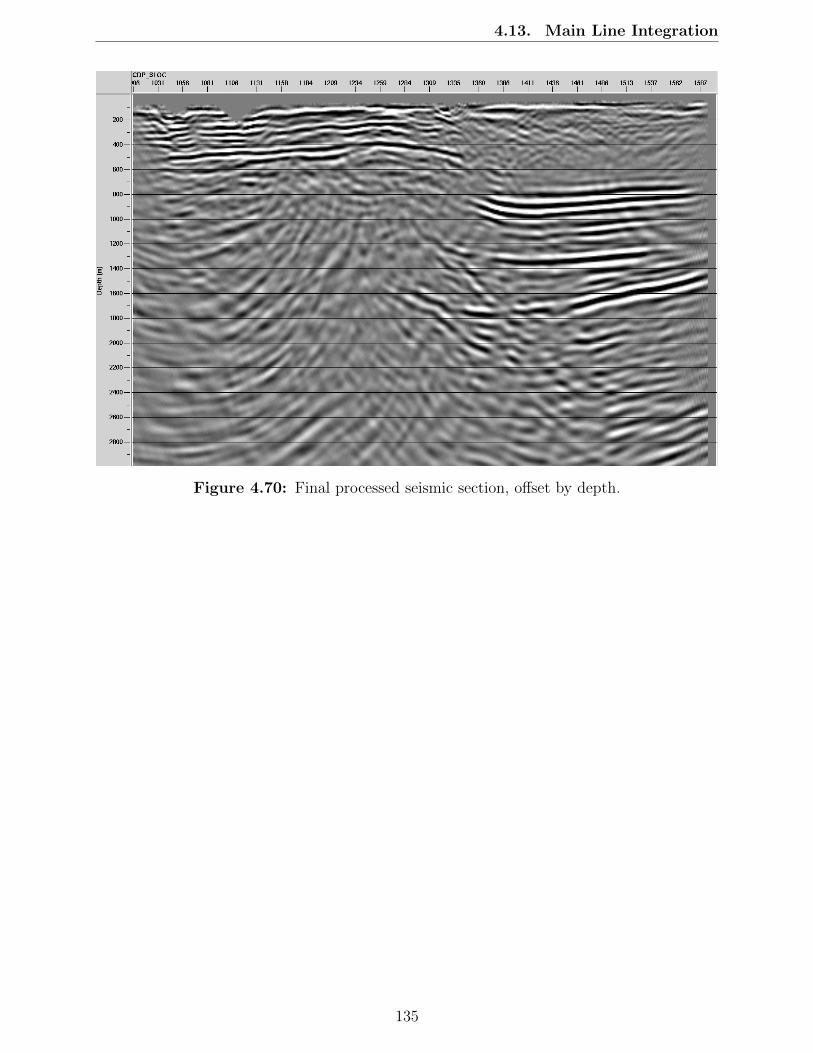
4.13. Main Line Integration
Figure 4.70: Final processed seismic section, offset by depth.
135

4.13. Main Line Integration
Figure 4.71: Interpreted geology and faulting over seismic image.
136

4.13. Main Line Integration
Alternative Interpretations: After collectively agreeing on a final interpretation, it isimportant to consider other possibilities that were concerned during the collective interpre-tive process. Other arguments were made in support of a normal fault rather than the reversefault observed in the seismic section. The final seismic image could still be further processedwhere we could potentially observe clear evidence of a normal fault. However we observedthe same reflectors prior to migration using multiple velocities through the subsurface, pro-viding evidence against a normal fault. The alternate interpretation would assume that theactivity caused by the fault is much younger because depositionally, the lithologies wouldhave to agree along the scarp. This subsided based on further seismic interpretation (dis-cussed previously) on the orientation of the fault and the fact that there was a missed shotover that blurred area which can potentially provide a inaccurate artifact. The anticlinalstructure folds over the fault and then is thrusted upward indicative of a reverse fault.
Gravity: Gravity provides the best supporting evidence in relation to the seismic sectionbecause the gravity method has a comparable depth of investigation. Gravity tells of thestructure of the Precambrian basement because of the high density contrast and also providesadditional information to the west of where the seismic line ended. Below in (Figure 4.72we see an integrated image where gravity is overlain on our seismic section providing furtherinsight to the geologic environment. Just like in our seismic image, we observe the samelithologies, cementing our interpretations along the section. These interpretations seem tofit perfectly, but some manipulation to the seismic data is consequently altered to fit itsgravity counterpart, and conversely, subtle features in the gravity data were compromised tofit the seismic. After scaling appropriately, the seismic interpretations are traced along thegravity line and the geologic contacts thereby overlain. This effectively shifts the orientationof the large reverse fault we see along the anticline. Our interpretations remain unaffected,but it is important to understand manipulation in case the depth of the layers or orientationof the fault were compromised.
Figure 4.72: Gravity over the finalized seismic image (Figure 4.70)
137

4.13. Main Line Integration
Figure 4.73 is an excellent representation of why integration is so valuable. Here we see twoviable solutions for the eastern part of our line. While both possible tectonically and geolog-ically, we need integration with another method with better resolution to make conclusionson the eastern part of our line.
Figure 4.73: Illustration of integration importance. Both geologic structures on the eastside of the anticline fit our gravity data. Without additional seismic data, the structure ispoorly constrained and both interpretations are viable.
138

4.13. Main Line Integration
Magnetotellurics: Magnetotellurics is our deepest method, recording differences in resis-tive and conductive layers in the subsurface. Because this is a passive method, utility wiresmade much of our data difficult to interpret along the seismic profile. We have included threeof our strongest sites providing a spatial distribution along the main line profile. Fortunately,the three less affected stations are over significant transition zones along the line, providinggreat supporting evidence to our previous data. The three stations visually provided by thered arrows in (Figure 4.74), sit on the east and west side of the line, and also directly over theanticlinal axis providing a transition zone between the resistive basement layer (dark) andconductive (light) sandstones. This method supports the geological representation concludedwith gravity and seismic data.
Figure 4.74: MT data over seismic profile showing the matching anticlinal structure.
Figure 4.75: MT data over seismic profile, providing additional evidence for the largethrust fault identified on the seismic section.
139
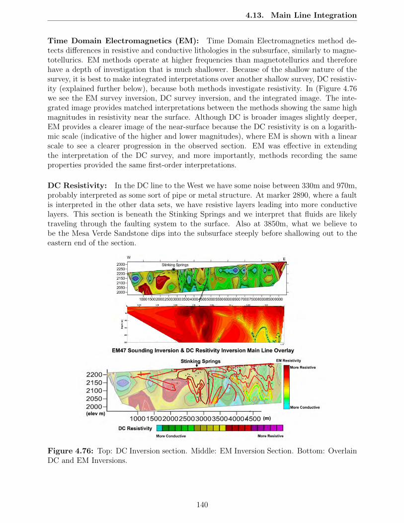
4.13. Main Line Integration
Time Domain Electromagnetics (EM): Time Domain Electromagnetics method de-tects differences in resistive and conductive lithologies in the subsurface, similarly to magne-totellurics. EM methods operate at higher frequencies than magnetotellurics and thereforehave a depth of investigation that is much shallower. Because of the shallow nature of thesurvey, it is best to make integrated interpretations over another shallow survey, DC resistiv-ity (explained further below), because both methods investigate resistivity. In (Figure 4.76we see the EM survey inversion, DC survey inversion, and the integrated image. The inte-grated image provides matched interpretations between the methods showing the same highmagnitudes in resistivity near the surface. Although DC is broader images slightly deeper,EM provides a clearer image of the near-surface because the DC resistivity is on a logarith-mic scale (indicative of the higher and lower magnitudes), where EM is shown with a linearscale to see a clearer progression in the observed section. EM was effective in extendingthe interpretation of the DC survey, and more importantly, methods recording the sameproperties provided the same first-order interpretations.
DC Resistivity: In the DC line to the West we have some noise between 330m and 970m,probably interpreted as some sort of pipe or metal structure. At marker 2890, where a faultis interpreted in the other data sets, we have resistive layers leading into more conductivelayers. This section is beneath the Stinking Springs and we interpret that fluids are likelytraveling through the faulting system to the surface. Also at 3850m, what we believe tobe the Mesa Verde Sandstone dips into the subsurface steeply before shallowing out to theeastern end of the section.
Figure 4.76: Top: DC Inversion section. Middle: EM Inversion Section. Bottom: OverlainDC and EM Inversions.
140

4.13. Main Line Integration
4.13.2 Water Flow Analysis
The determination of water flow patterns in Chromo is based on the structure analysis aboveand an understanding of the larger geologic picture detailed at the beginning of the report.Because our data was collected in two dimensions across only one line, it is impossible tofully characterize the hydrothermal flow patterns. Thus, we present multiple hypothesis forwater flow patterns in the area. Hypotheses are presented in order of most likely to leastlikely. Refer to the recommendations section for further information on the surveys andadditional studies suggested to further characterize fluid flow in the region.
Water Transport from Northwest
The town of Pagosa Springs sits approximately 25 miles northwest of Chromo. The currentworking hypothesis based on the 2013 Colorado School of Mines Geophysics Field Campreports for geothermal activity in Pagosa Springs is an upwelling of water traveling alongfault zones from the northeastward San Juan mountains ([35]). The source of the wateris meteoric water traveling down to the Precambrian basement through fault and fracturezones. Due to the existence of known faults transporting water from the source in the SanJuan mountains to Pagosa Springs and faults running parallel to the axis of the ArchuletaArch, it is plausible that the same geothermal seen in Pagosa Springs continues downwardtowards the Chromo area.
Basement Transport Geothermal water from Pagosa Springs traveling to Chromo throughthe heavily fractured Precambrian basement rock is the most likely scenario for fluid trans-port from the source location (Figure 4.77). The upwelling of hot water along large faultzones suggests a transport system characterized by local springs with complex interconnectedfracture systems. Due to the age of the crystalline basement, it is a far more likely candidatefor the presence of an extensive fracture system capable of transporting geothermal water.Sedimentary layers deposited during the recession and transgression of the intercontinentalseaway are far less likely to have an extensive fracture system because their age is youngerthan our dating of the faulting and folding structural events. Basement transport also allowsfor geothermally heated water in a temperature range depending on the depth of fracturetransport, resolving why the temperature in the springs at Pagosa Springs and Chromo dif-fers. While the exact source of the geothermal water is unknown, the depth of our basementrock and size of the fault identified on our Main Line supports the full range of temperaturespresent in the area regardless of the presence of remnants of a magmatic source body. Oncethe water is in the Chromo area, it flows up to the surface along the large fault identifiedalong our Main Line, traveling along the main fault as well as the smaller fracture zones andnormal faults in the near surface under the stinking springs area.
141

4.13. Main Line Integration
Figure 4.77: Water transport through the fractured crystalline basement.
Sedimentary Transport As a secondary option for fluid flow between Pagosa Springsand Chromo, we consider the possibility of fluid traveling through the more shallow sedi-mentary layers of the subsurface (Figure 4.78). While less likely, geothermal water transportthrough shallow, porous sedimentary layers like the Dakota Sandstone is feasible. Forma-tions such as the Morrison and Mancos Shale are unlikely candidates for water transportsimply because of their natural impermeability. The Dakota Sandstone, however, has botha higher permeability and porosity, indicating that it is more permissive of water flow. TheDakota sandstone, a known aquifer, is the most likely layer for geothermal water to partiallyor fully saturate. While imaging Dakota sandstone fracture zones or measuring rock physicsparameters like porosity were not considered in the scope of this experiment, they couldindicate water flow from Pagosa Springs to Chromo. Water flow in the Dakota sandstone orrelated rock units would likely require some additional heating source, as the shallow depthis unlikely to produce moderate geothermal temperatures. Similarly to basement transport,water reaching the Chromo area would rise to the surface via the fractured near surface zoneor along the plane of the thrust fault.
142

4.13. Main Line Integration
Figure 4.78: Water transport through the Dakota Sandstone.
Water Transport from Northeast
Regardless of whether the water makes a transit through the Dakota Sandstone or thePrecambrian basement, another hypothesis for the primary direction of fluid flow is a directpassage from the northeastward San Juan mountains to Chromo, skipping the Pagosa Springsarea entirely. This could throw forward several proposals for subterranean water movementin the area entirely: a primary channel could connect the San Juan mountains and Chromowhile a smaller thread could link Pagosa Springs and a section along this channel. Or, twodifferent channels could link the towns to the mountains entirely. We consider a direct linkagebetween the source location and Chromo to be our weakest hypothesis, as the orientationof geologic structures does not directly connect the two locations. Faults intersecting theArchuleta anticline at an angle would be necessary for fluid transport directly from theNortheast, and such structures are unlikely to from known ancient stress regimes. However,if additional surveys proved inconclusive, direct transport could be considered as an option.
143

4.13. Main Line Integration
Figure 4.79: Hypothetical Water PassagesA: Passage from San Juan Mountains to Pagosa Springs to Chromo.B: Direct passage from mountains to Chromo.
4.13.3 Integration Conclusions
We suggest the model of fluid flow from the northwest Pagosa Springs region through fracturesystems in the crystalline basement rock as the most likely scenario for the appearanceof geothermal springs in the Chromo region. This model fits a wide array of unknownvariables including source details and temperature differences. Two additional models ofnorthwest flow in shallow sedimentary layers and direct northeast flow from the source areposed as alternative models. Water is likely rising to the surface through the identified largereverse fault and fracture system across our Main Line, regardless of larger-scale transportorientation. Further characterization through additional surveys, geological mapping, androck physics are needed to determine more exact details of the regional geothermal system.
144

CHAPTER 5
STUDENT SITE
5.1 Student Site Introduction
Student site surveys have been a part of the CSM Geophysics Field Camp for a number ofyears. Traditionally, the purpose of the student site is to demonstrate the abilities of thestudents to design and carry out their own geophysical surveys. This not only gives confi-dence to the students in performing geophysical investigations, but also demonstrates to thefaculty the culmination of the student’s knowledge.
This year’s Student Site was chosen based on the interesting geophysical problem of find-ing buried well casings. The leaking well called “Flowing Well” is expressed on the surfaceand was first considered a possible Student Site location after the geologic tour of Chromo.Flowing Well and other wells in the area have corroded well casings that can be easily pickedup by some of our methods. The methods that our team decided upon are listed below andwere chosen based on ability to image the well casings or water flow.
• Ground Penetrating Radar
• Hammer Seismic
• Self Potential
• DC Resistivity
• Electromagnetics (using EM-47)
• Magnetics
Because of the depths of investigation of these methods as well as the individual propertiesthat each method senses, the data from the Student Site cannot be interpreted for subsurfacestructure of the Chromo area except for near surface characterization. The data acquisitionand processing will be able to locate additional wells and provide a signature from whichsimilar wells in other areas can be located. Basic shallow interpretations of geologic structureare also analyzed by the Student Site methods. This information can benefit residents inthe area, as these well casings and leaking wells are undesirable and can cause pollutants.
145

5.2. Ground Penetrating Radar
5.2 Ground Penetrating Radar
5.2.1 Survey Location
There was a 50.0 meters by 50.0 meters survey grid completed within the northwest endof the student site Figure 5.1. Missing data points can be attributed to the running waterflowing through the middle of the site where the equipment had to be carried over; themissing data represented with the blue line in Figure 5.2.
Figure 5.1: Student Line GPR Survey Location.
146

5.2. Ground Penetrating Radar
Figure 5.2: Line 3 of the Student Site.
5.2.2 Survey Design
There were 11 lines, 50.0 m in length, taken 5 m apart, running in the area where theSW-NE grid at the student site would eventually be located. The location was chosenbecause GPR needs fairly mild topography to get accurate survey depths and Flowing Wellis topographically difficult to get to, even without the GPR.
5.2.3 Processing
For the Student Site processing, we viewed the data in Ekko View 2. We started by applyingan automatic gain control (AGC) and shifting the colormap to an easier to interpret grouping.We were able to extract and analyze anomalies (hyperbolas) and to use those hyperbolas toget velocities of the area.
5.2.4 Interpretation
The GPR lines at the Student Site do not yield any pertinent information. We did notget accurate lengths on the lines because data acquisition required pausing collection andwalking over a creek. The lines were also not an accurate length because the odometer wasnot calibrated correctly. We did not see anything of interest because the GPR has a veryshallow depth of investigation; it only sees variations in the ground and it was not a goodarea to walk the GPR unit. There are stretches in the data, shown to the right of the blueline in Figure 5.2, but these are seen when the GPR is picking up multiples from the samesignal creating illusionary reflectors.
5.2.5 Sources of Error/Uncertainty
Possible sources of error and uncertainty on this set of GPR data is abundant. The notestaken in the field do not specify exactly where they picked up the GPR and walked it acrossthe creek, the data has some spots where it looks like the wheel was spinning and the devicewas not moving, and the topography was not ideal. There also could have been device errorfrom improper settings or broken internal parts.
5.2.6 Conclusion
In conclusion, GPR at the Student Site was not used further due to the nature of the site.This data collection was mostly a test to see if doing anymore GPR here would be helpful.We concluded that it would not be a good use of time to continue collecting data over thefinal grid. This data collection served its purpose.
147
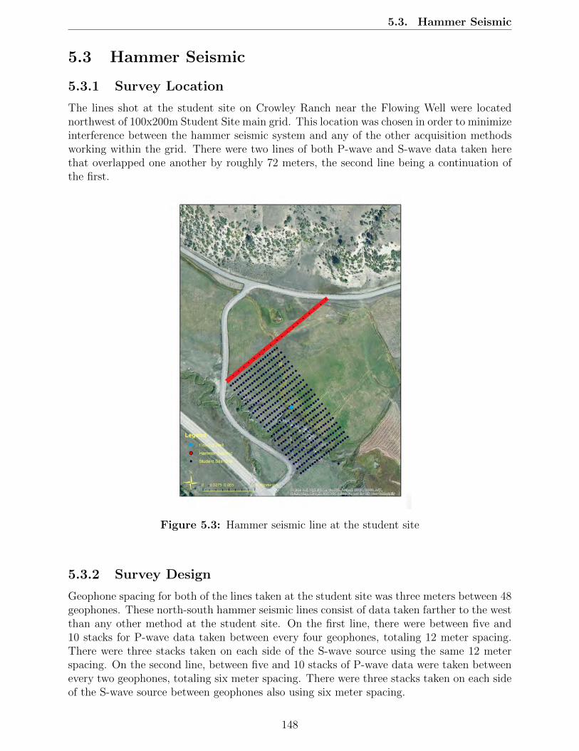
5.3. Hammer Seismic
5.3 Hammer Seismic
5.3.1 Survey Location
The lines shot at the student site on Crowley Ranch near the Flowing Well were locatednorthwest of 100x200m Student Site main grid. This location was chosen in order to minimizeinterference between the hammer seismic system and any of the other acquisition methodsworking within the grid. There were two lines of both P-wave and S-wave data taken herethat overlapped one another by roughly 72 meters, the second line being a continuation ofthe first.
Figure 5.3: Hammer seismic line at the student site
5.3.2 Survey Design
Geophone spacing for both of the lines taken at the student site was three meters between 48geophones. These north-south hammer seismic lines consist of data taken farther to the westthan any other method at the student site. On the first line, there were between five and10 stacks for P-wave data taken between every four geophones, totaling 12 meter spacing.There were three stacks taken on each side of the S-wave source using the same 12 meterspacing. On the second line, between five and 10 stacks of P-wave data were taken betweenevery two geophones, totaling six meter spacing. There were three stacks taken on each sideof the S-wave source between geophones also using six meter spacing.
148

5.3. Hammer Seismic
5.3.3 Processing
Refer to Processing for Main Line of Hammer Seismic.
5.3.4 Interpretation
Hammer seismic refraction interpretation consists of these following steps.
1. Choosing the refraction method.To begin with the refraction analysis, we have to choose the reflection method that fitwith the local geological setting in the area. Three common methods are (1) a singlesubsurface interface, (2) two horizontal interfaces, and (3) dipping interfaces
2. Velocity calculationFrom the shot profiles, we calculate the velocity of the top layer (v1) and the secondlayer (v2) by using
v =∆distance
∆time(5.1)
3. Thickness calculationOnce we know the velocity of the top layer and underneath layer, we can calculate thethickness of the top layer by using
h1 =ti2
V2V1
(V 22 − V 2
1 )12
(5.2)
where h1 and v1 are the thickness and velocity of top layer, respectively.v2 is the velocity of bottom layer.ti is the intercept time from the time-distance plot for each shot:
In the case of double geological interfaces model, we need to calculate v3 of the thirdgeological layer and the thickness of the second formation could be found by using theequation below.
h2 =
(ti2 −
2h1(V23 − V 2
1 )12
V3V1
)V3V2
2(V 23 − V 2
2 )12
(5.3)
where; h1 and v1 are the thickness and velocity of top layer, respectively.h2 and v2 are the thickness and velocity of middle layer, respectively.v3 is the velocity of bottom layer.ti is the intercept time on the from the time-distance plot for each shot.Please be note that these models have an assumption that v3 > v2 > v1 .
149

5.3. Hammer Seismic
4. In case that we suspect the formation is dip in some specific direction, one could use thethe dipping interfaces model to figure the dip angle of the layer. In this 2014 geophysicsfield camp, we suspect the dipping formation exists along the line at the student siteand main line. Thus, in order to make the result as close to the natural setting aspossible, we apply this model and calculate the dip of the formations. To begin withthe dip calculation, we need to calculate the velocity of the interested dipping layer atthe down-dip position and the up-dip position by using
v =∆distance
∆time(5.4)
Then, we define the parameter called md and md which are the inverse of the velocity ofdipping layer at down-dip and up-dip position respectively.
slope = mu =1
V2R(5.5)
slope = md =1
V2F(5.6)
After that, we use these two following equations to figure out the dip of interested subsurfacelayer.
θic =arcsin (V1md) + arcsin (V1mu)
2(5.7)
β =arcsin (V1mu)− arcsin (V1md)
2(5.8)
Detailed explanation on each variable and model could be found in the theory and back-ground part of hammer seismic.
After analyzing the P-wave velocities and calculating the depths of the second layer werealized that we were getting very shallow depths. We realized that the shallow depths werenot actually identifying the depth of the second layer but rather showing us the depth ofthe water table. When we looked at the S-wave data and calculated the S-wave velocitieswe confirmed that the second layer was actually deeper than the P-waves showed. As shownin Figure 5.4 we can see that the water table sits about two meters underground on top ofan unsaturated layer. The depths that were calculated for the water table stayed consistentalong the entire line as well. The S-wave velocities that were calculated showed that thedepth of the second layer was changing along the line. Using Equation 5.8 we were able tocalculate the different dips of the second layer and make a model of how it changes alongthe line, as shown in Figure 5.5. By looking at different velocity models along the line wecan saw that the second layer is dipping more towards the north east end of the line witha dip of about 1.5 degrees. It then begins to dip up at about 1 degree. The peak that thesecond layer reaches is at about 6 meters from the surface. From there it begins to gentlyslope back down at about 0.75 degrees. By combining the information from the P-waves andthe S-waves we are able to for the model shown in Figure 5.6 that shows the location of thewater table as well as how the second layer is changing along the line.
150

5.3. Hammer Seismic
Figure 5.4: Subsurface of the Student Site using P-waves.
151

5.3. Hammer Seismic
Figure 5.5: Subsurface of the Student Site using S-waves.
152

5.3. Hammer Seismic
Figure 5.6: Geological model of the student site combining information from the P-wavesand the S-waves.
5.3.5 Sources of Error/Uncertainty
Refer to Sources of Error and Uncertainty for Main Line of Hammer Seismic.
5.3.6 Conclusion
In conclusion, using Hammer Seismic at the Student Site was beneficial. From P-waveswe extracted knowledge about the water table in the area and from the S-waves the firstrock layer below the dirt. Using our changing velocities throughout the line we were ableto calculate different dips to determine the general shape of the sub-surface. By combiningthese two pieces of information we were able to make a model of the dirt-rock contact in thesub-surface.
153

5.4. Self-Potential
5.4 Self-Potential
5.4.1 Survey Location
A self-potential survey was conducted on the Flowing Well student site, pictured in Fig-ure 5.7. A total of 15 lines of self-potential data were acquired, with two additional highresolution lines over the known wells in the area. This acquisition is sensitive to the flowof fluid underground as well as the corrosion of metallic bodies in the subsurface. Acquireddata from these two types of responses can be utilized to determine the location of corrodedwell casings that were visible at the suface of the Flowing Well student site.
Figure 5.7: Aerial photo of the SP survey grid at the Flowing Well student site.
154

5.4. Self-Potential
5.4.2 Survey Design
The self-potential survey set up in a grid over the Flowing Well student site is pictured inFigure 5.7. This was comprised of a total of 10 lines, and two high-resolution lines overknown wells. Figure 5.8 shows the basic survey setup of a self-potential acquisition; one ofthe pictured electrodes is fixed as a base station to correct for drift, while the roving electrodeis used to take measurements of potential difference (voltage) at different measuring stationswith a given spacing.
Figure 5.8: General setup of self-potential acquisition. [5]
Equipment
Self-potential involves measuring the change in potential from a base to a roving electrodeacross a natural electric field produced by water carrying excess charge flowing as well asthrough the corrosion of metallic bodies in the subsurface. This is done to acquire anidea of streaming potential distributions across a lateral distance over the student site area.To successfully measure these voltages, or streaming potential, the following equipment isrequired:
Table 5.1: Required equipment for 2D self-potential acquisition.
Item Purpose2 non-polarizing electrode Type: (Pb-Pb)
Reference-provides means by which to account for drift;buried at beginning location and left stationary duringacquisition (base station)Roving-takes station-to-station readings of difference inpotential from reference to current station
500 m reel of cable Connects electrodes to each otherMultimeter Used to measure U (voltage, or change in potential)
across reference/roving electrodesShovel To dig holes and ensure proper electrode contact with ground
155

5.4. Self-Potential
Figure 5.9: Example image of non-polarizing electrodes equivalent to thoseused in the Flowing Well self-potential ac-quisition [3].
Figure 5.10: Example image of a multi-meter that measures self-potential (or volt-age) as was done in the Flowing Well self-potential acquisition [2].
Parameters
Table 5.2 outlines the specific parameters that were used during the self-potential acquisitionat the Flowing Well student site pictured in Figure 5.7:
Table 5.2: Parameters used for DC Resistivity student site acquisition
Parameter ValueStation spacing 5 mLine spacing 10 mLine length 100 mStations per line 21Total lines 15 running EW
156

5.4. Self-Potential
5.4.3 Processing
Initially, self-potential data collected in the field was inspected in a spreadsheet to qualitycontrol the data. Profiles of the lines of self-potential data collected over the student sitewere plotted using Grapher for initial inspection. Erroneous data points found were manu-ally eliminated and coordinates were added to the data based on the grid laid out over thestudent site. This was then saved as a *.dat and *.bln file to be imported into the Surferprogram.
An arbitrary 140 meter by 100 meter grid corresponding to the dimensions of the self-potential site (Figure 5.7) was created in Surfer. The data were imported into Surfer andadded to the corresponding grid points manually due to an error in GPS data. Surfer wasused to create two contour maps of streaming potential over the Flowing Well area on thestudent site using interpolation; one was made using the maximum values of the potential,and one using minimum values of self-potential measured. The high resolution data collectedover the wells were added, helping accentuate the response of the two wells and regularizethe color scale. This contour map was then overlain with the locations of the stations of theSP grid, pictured in Figure 5.11. This image was then placed on top of a Google Earth imageof the student site to highlight the correlation of the self-potential with the surface features,resulting in a ground surface map of the potential over the Flowing Well site (Figure 5.12).
The interpolation technique used by the Surfer program to fill in the self-potential valuesin the areas between data points is called kriging. This is a method in which interpolatedvalues are obtained using a Gaussian process that is governed by prior covariances. Thisis done instead of using a line of best fit that optimizes smoothness of fitted values, sincethe spatial variation of the data is more important than continuity in self-potential data.Kriging gives an unbiased, linear prediction of intermediate values, ignoring the criteria forsmoothness that many other interpolation techniques tend to incorporate. Kriging varianceis instead a function of the location of the data points, not their values, meaning that astructural model reflecting the spatial variability of the data points collected is fitted to thedata instead of value-based smoothing [46].
Using Grapher, some of the self-potential lines were plotted atop DC resistivity lines thatwere also at the student site to show the correlation between the measurements and to makeconclusions based on incorporation of additional information. The resulting images will beincluded in the DC resistivity student site discussion.
157

5.4. Self-Potential
5.4.4 Results
Figure 5.11 displays the resulting interpolated surface contour map of the self-potential mea-surements taken at the student site, showing the spatial distribution of potential differencesacross the self-potential grid over the Flowing Well student site.
Figure 5.11: Grid of self-potential ground-surface contour plot of potential signals acquiredover the student site.
Figure 5.12 shows the ground surface contour map of the self-potential on top of the FlowingWell site.
Figure 5.12: Aerial photo of the SP ground-surface contour plot atop the Flowing Wellstudent site.
158

5.4. Self-Potential
Figure 5.13: 3D kriging result of the SP student site.
Figure 5.14: 3D topography of the SP student site.
159

5.4. Self-Potential
5.4.5 Interpretation
Wells have a strong negative electric potential response, especially when corroded and ori-ented vertically [40]. Figure 5.11 shows strong negative electric potential responses over thetwo wells, located at approximately (45, 2.5) and (100, 50) on the grid. The small span ofthe voltage response is due to the fact that these measurements were taken at the surface,where the wells were located. If these wells were deeper, the response would have spanned alarger area.
Roughly speaking, positive voltages come from water flowing upwards, while negative re-sponses represent where water is flowing down. On the eastern end, the more shallow watertable gave a positive anomaly, while the western end had water up to 5 meters below theground surface, giving a negative response due to a decrease in dissolved oxygen withinthe pore fluid at that depth [40]. In Figure 5.12, the stream running through the centerof the student site is distinguishable, separating the more positive potential changes fromthe negative potentials. The same stream can also be seen cutting across between the pos-itive and negative areas in the 3D interpolation image with topography added in Figure 5.13.
While the overall trend of responses is positive on the eastern end and negative on the west-ern end, there are breaks in SP values because the topography is non-uniform, shown inFigures 5.13 and 5.14. If the generalization is made that the irrigation water at the surfaceis flowing to the southwest, the underground water table may be doing trending the sameway. While the student site is a significant distance away from the main line, if there is aregional trend of water flow, this may help determine where water is traveling undergroundand provide more information about the geothermal system in Chromo.
5.4.6 Sources of Error/Uncertainty
The GPS data collected over the student site was erroneous, and so the resulting griddedimages are not exact. The grid was fit as best as possible, but is likely not exact.
Lightning and transient current flow in the ionosphere cause induction of telluric currents inthe subsurface. These currents can cause unwanted noise in the self-potential data acquired.Unaccounted-for conductive items in the subsurface may result in an inaccurate reading ofself-potential. Induction due to powerlines, utilities and other conductive objects could alsocontribute to error in voltage data. A magnetometer can be used to record correlated mag-netic signals to account for this uncertainty [39].
Interpolation, while useful in filling in unknown values, is only an estimate. In reality, valuesmay vary less smoothly and there could be undetected anomalies whose responses do notspan enough area to be detected on each line. Any area outside of the lines incorporated istherefore erroneous and not a perfect representation of the actual self-potential in those areas.
160

5.4. Self-Potential
5.4.7 Conclusion
Self-potential measures voltage differences across lateral distances to obtain an idea of thefluid flow in the subsurface as well as to distinguish corroding bodies that are present un-derground, both of which are natural sources of telluric currents that produce electric fields.
Both the corroded well casings present on the Flowing Well site were located using theself-potential acquisition method, and a relative trend of fluid flow towards the southwest islikely given the results of this survey. The water table was found to be within 5 meters ofthe surface on the western end of the student site, while the positive voltages on the easternend indicated more shallow saturated areas.
161

5.5. Direct Current Resistivity
5.5 Direct Current Resistivity
5.5.1 Survey Location
Figure 5.15 displays the DC resistivity grid, in red, set up at the Flowing Well student site.Grid lines were spread 20 meters apart in the E-W direction and 40 meters apart in theN-S direction. The lines were approximately 155 meters long, with 32 stations per line. Theknown well is marked on the surface by the blue marker in Figure 5.15.
Figure 5.15: Aerial photo of the DC survey grid at the Flowing Well student site.
5.5.2 Survey Design
As was done for the main line of DC resistivity, two current-injecting electrodes were used torun current through the subsurface, while potential electrodes measured the voltage acrossa given distance. This was done to obtain a geometric distribution of apparent resistivityunderground, giving an idea of fluid content in the subsurface as well as the location of wellcasings underground. Detailed survey design is covered in the main line section pertainingto DC resistivity.
Equipment
A detailed outline of the equipment used for the Flowing Well DC resistivity data collectioncan be found in the section describing the main line DC resistivity acquisition; the same
162

5.5. Direct Current Resistivity
general equipment was used at both sites to carry out the acquisition. In the case of thestudent site, however, only 32 electrodes were used per acquisition, with one reel on eachside of the midpoint of acquisition.
Parameters
Table 5.3 outlines the survey parameters used in the DC resistivity Flowing Well site acqui-sition.
Table 5.3: Parameters used for DC Resistivity student site acquisition.
Parameter ValueArray type WennerElectrode spacing 5 mImposed current 200 mAAcquisition time 0.30 secondsDelay time 0.30 secondsLength of single acquisition 155 mGrid dimensions 20 m in the short (EW) direction
40 m in the long (NS) directionwith 5 lines in each direction
Measurements per acquisition approx. 1302 stacks per measurement
Approximate depth of investigation 30 m
5.5.3 Processing
In addition to the processing techniques that were done on the data DC resistivity main line(extermination of points and RMS error analysis), topography data had to be matched andoriented to fit each inverted line of acquisition at the Flowing Well student site. However,no image-guided inversions were done on the DC resistivity data for the student site.
As was done for the DC main line, the student site lines 1 through 10 were inverted using anL2 norm instead of the robust inversion, with three iterations, and a vertical-horizontal ratioof 1. Damping factors incorporated were default parameters: an initial damping of 0.15, aminimum of 0.02, with the 1st layer value set at 5.0.
The 2D line inversions that were created were then oriented in (x, y, z) space with respect toeach other to form a 3D arrangement of slices, or sections. Using a program called Voxler,an isotropic interpolation method was used to fill in areas between lines of acquisition withprobable resistivity values, giving a 3D distribution of resistivity. Slivers of resistivity ata given depth could be extracted from the resulting cube for interpretation, and specificresistivity values could be isolated as well. To understand the geometry of the student site,the cube was separated into depth slices. Inspecting the resistivity at the surface will give anidea about the response of the wells and the relative conductivity of the surrounding area.
163

5.5. Direct Current Resistivity
5.5.4 Results
Three separate unguided inversion results from the student site are pictured below:
Figure 5.16: Line 1 of DC acquisition at student site.
Figure 5.17: Line 3 of DC acquisition at student site.
164

5.5. Direct Current Resistivity
Figure 5.18: Line 8 of DC acquisition at student site.
165

5.5. Direct Current Resistivity
Figure 5.19: Results of 3D interpolation of DC Resistivity data at Flowing Well studentsite. Data is shown as depths-slices at 7.5 m intervals. There is a general increase inresistivity with depth.
Figure 5.20: 3D slice at 30m depth picturing the more resistive ridges.
166

5.5. Direct Current Resistivity
5.5.5 Interpretation
The orientation of the three most pertinent individual DC resistivity lines with respect toeach other is shown in the appendix. Line 1 is on the edge of the student site running roughlyNS, but does not intersect Well 2, which was off of the site located at (339623, 4098547)UTM. Lines 3 and 8 are perpendicular, and both bisect the DC resistivity survey grid (Line3 is NS, Line 8 is EW) and almost intersect the first well at (339429, 4098066). These arealso pictured in Figure 5.15.
At the student site, there is an increase in resistivity with depth, as shown in the resultssection in Figures 5.16, 5.17, and 5.18. This overall increase with depth can also be seen inFigure 5.19, and is due to the water saturation at the surface from the creek that was recentlydammed in the area. In addition, there is a general trend of decrease in conductivity to theSW. Since fresh water is non-conductive, water could be flowing along the two NS trendingresistive ridges pictured in Figure 5.20 just as the resistivity values trend along these at 30meters depth. These could also be attributed to cultural noise if there are unaccounted-forbodies in the subsurface. Horizontal features also would not appear in the self-potentialresponse, and so this may be a cause of error [40].
In the pertinent DC lines shown in Figures 5.16, 5.17, and 5.18, the response of the wellsis detectable around 1.2 Ω ∗ m, since these are old and their signature is mainly basedon corrosion of the pipe. As depth increases, it is possible to distinguish more conductiveareas that appear circular in shape on the depth slices seen in (Figure 5.19), indicatingthe presence of a cylindrical, vertical conductive body. Since the resistive unit present atthe bottom of the line sections is being bisected at the approximate location of each of thewells, this indicates that the corroded casings could be causing a more conductive responsethan would be expected at that depth (Figures 5.16, 5.17, and 5.18). However, this is notconclusive because the anomalies are on the same order of resistivity values as surroundingmeasurements.
5.5.6 Sources of Error/Uncertainty
Sources of error and uncertainty associated with DC resistivity acquisition are outlined indetail in the section of this report describing the main line of DC resistivity.
For the Flowing Well site, some lines had anywhere from 28 to 32 electrodes working ata time. While this discrepancy would not incorporate significant error in the main lineof DC resistivity due to the scale and geometry of that problem, this is a cause for un-certainty in the student site lines. This is because the Flowing Well DC lines were eachacquired separately from one-another and were relatively short, while the main line con-sisted of laterally-overlapping, stacked acquisitions.
Error could also arise from the equipment of other crews working at the site simultaneously.Other methods require coupled geophones, current loops, and other sources or sinks of cur-rent flow. These could incorporate noise into the data collected if these were close enoughto the DC resistivity survey at any point during acquisition.
167
5.5. Direct Current Resistivity
5.5.7 Conclusion
DC resistivity imaging uses injected current and measured voltage differences to acquire adistribution of resistivity in the subsurface, which is then inverted to obtain an image of trueresistivities. Resistivity is an intrinsic rock property that is unique to the physical charac-teristics of a given geologic formation, including saturation and rock type.
At the Flowing Well student site, there is an overall trend of an increase in resistivity withdepth. Conductive, corroded wells can be seen in the resistivity tomograms resulting frominversion as more conductive, vertically-oriented areas. These vertical wells can also be seenat depth in the 3D resistivity images created: their signature on the surface depth slices isa decrease in resistivity over a circular area. The locations of these wells are as follows:
Well 1: (339429, 4098066) UTMWell 2: (339623, 4098547) UTM
The self-potential data overtop the DC resistivity lines at the student site shows a correla-tion between the conductive areas in the tomograms where the wells are situated and thelarge negative potential responses in the SP profiles (Figures 5.21, 5.22, and 5.23). Thisconfirms the location and vertical orientation of the two known wells. Consistently, areaswith higher resistivity showed higher readings for potential differences, while more conduc-tive areas showed low voltage values, due to the shallow water table in the Flowing Wellarea. A general southwest trend of fluid flow is thought to be detected in both self-potentialand direct current resitivity processed data.
Future prospects include a full 3D inversion of the self-potential data constrained by thedirect current resistivity, which would help distinguish the geometry, volume, and precisedirection of water flow.
168
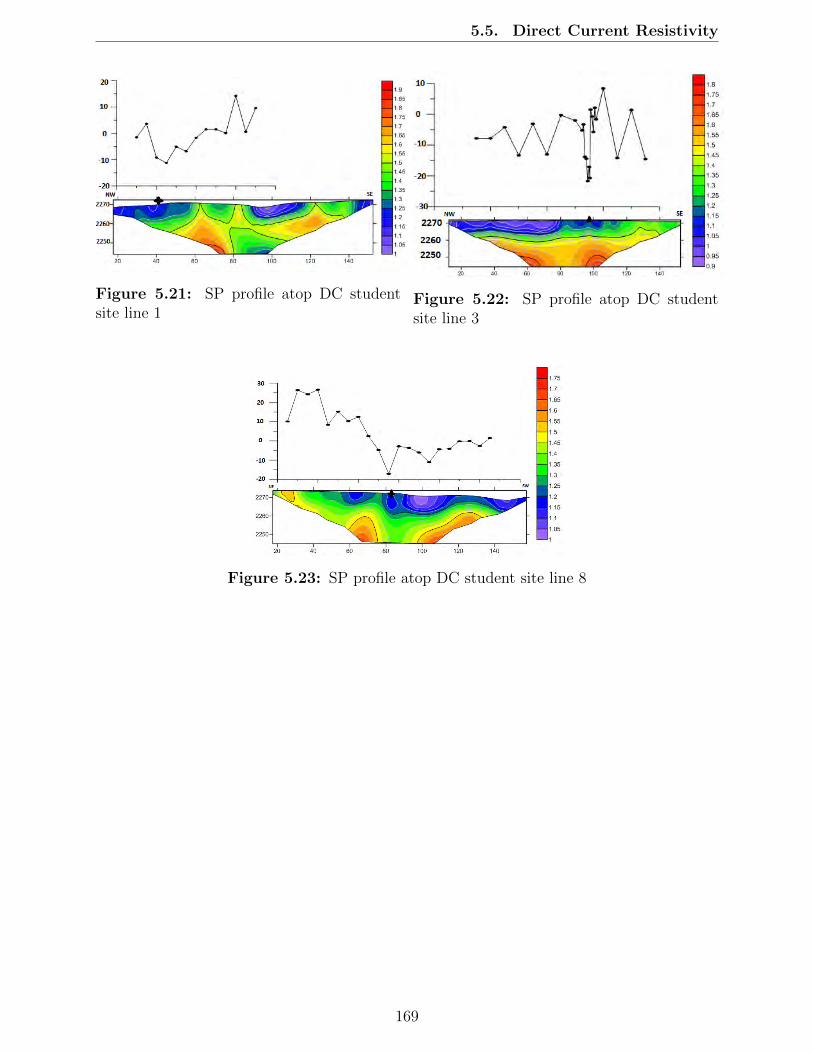
5.5. Direct Current Resistivity
Figure 5.21: SP profile atop DC studentsite line 1
Figure 5.22: SP profile atop DC studentsite line 3
Figure 5.23: SP profile atop DC student site line 8
169

5.6. Electromagnetics
5.6 Electromagnetics
5.6.1 Survey Location
At the Student Site, we also used the EM-47. The electromagnetics survey consisted of an80 meter by 80 meter grid centered around Flowing Well. The corners of the grid werelocated at flags C6, C14, S14, and C14 (where the current loop was located). Readings wereattempted every ten meters, terrain permitting. Readings were not taken within ten metersof the outer coil. Near Flowing Well, readings were taken every five meters. Locations wererecorded in UTM coordinates using handheld GPS and later correlated using differentialGPS at flag markers.
Figure 5.24: Map displaying the EM Student Site survey grid and coil location.
Figure 5.24 displays the EM survey coil location with labeled corners. The yellow markersindicate where EM-47 readings were taken.
5.6.2 Survey Design
The Student Site survey was larger than that of the EM sites along the main line in anattempt to take more readings within a larger area. The 80 meter square grid allowed forthe largest possible grid with the available equipment while also imaging an increase depthof investigation. Flowing Well was the center of the grid for optimum EM readings of thewell and surrounding geology.
A total of 47 readings were taken within the grid. Originally, we planned to take read-ings every ten meters, skipping every other five meter-spaced flag, since they had a spacingof five meters; however, given the uneven terrain within the grid, several planned readinglocations had to be skipped because we were unable successfully level the EM-47. An ad-ditional seven readings were taken around Flowing Well for a better understanding of thesubsurface immediately surrounding the well.
170

5.6. Electromagnetics
The first readings were taken directly above Flowing Well. Three readings were taken at285Hz, 75Hz, and 30Hz. The remaining locations only had two readings taken at 285Hz and75Hz. The 30Hz reading was abandoned because the data from the 285Hz and 75Hz was soclean, a 30Hz reading would have been superfluous.
The current was kept at 2.5Amps when at 285Hz and 3.0Amps for 75Hz for consistencywith the readings taken on the main line. Only the z-component was taken at each site. Theremaining settings are as follows,
• Coil Type was set at 3D-1
• Turn Off Time was set at 5.0µs
• Transmitter Dimensions was set at ≥ 40 & MULTI-TURN
• Integration Time was set at 30s
• Gain was set at 1
• Comp Value was set at 1
For additional settings refer to the Appendix.
The recordings began with station 114 and recorded to station 209 under Operator 10. Eachreading location had two corresponding station readings given the two frequencies used, withthe exception of the first location since a 30Hz frequency reading was taken as well.
5.6.3 Processing
Prior to processing, the raw data had to be converted from mV to nV/m2. The MATLABcode used to convert the data can be found in the Appendix. Any test readings were alsoremoved prior to processing. Station 125 was the only test reading removed from the EMStudent Site data set.
The converted data was processed using the program IX1D. IX1D called for inputting the
171

5.6. Electromagnetics
data in nV/m2 with their corresponding times in milliseconds (see Appendix for frequencytimes). Since the EM-47 does not record an error, a baseline error percentage of 5.0% wasused for all Student Site data.
Figure 5.25: Resisvity-Time plot for EM reading taken at flag M13.
IX1D initially displays the data as a function of Resistivity vs Time. Figure 5.25 is anexample Resistivity-Time plot from flag M13. The red markers represent the data taken at285Hz and the blue markers represent the data taken at 75Hz. From these plots, a smoothmodel was estimated using 200 layers, a minimum depth of 1.0 meter, a maximum depthof 200.0 meters, and a starting resistivity of 70.0Ωm. If the smooth model had an RMSgreater than 20%, then the inversion was modeled by hand to achieve the lowest possibleRMS percentage.
The resulting inversions were saved and exported as an XYZ Model File. The exportedresistivity, depth, and location data was plotted in MATLAB, with resistivity plotted inlogarithmic time, for each SW to NE Student Site survey line (see Appendix for MATLABcode).
Figure 5.26 is the product of six EM readings taken on line 9 of the Student Site. Thereading locations are marked with the vertical black dots. The seven resulting lines werecombined in a three dimensional layered plot for ease of interpretation.
172

5.6. Electromagnetics
Figure 5.26: Student Site plot displaying the changes in resistivity for line 9E-9Q.
5.6.4 Interpretation
Figure 5.27 exhibits the seven two dimensional resistivity plots. In nearly every 2D plot, twothin conductive layers are seen around 100.0m and 135.0m which could indicate the presenceof water.
Figure 5.27: Three dimensional model created layering the Student Site resistivity lineplots.
173

5.6. Electromagnetics
Figure 5.28: 2D resistivity line plot with Fol-lowing Well for line 11E-11Q.
Figure 5.29: 2D resistivity line plot 20.0mSE of Following Well for line 13E-13Q.
When looking at the resistivity line plots individually, Flowing Well is seen with a moreconductive spot directly beneath the top of the well. This is most obviously seen in Figure5.28. The area almost directly below Following Well is more conductive than the surroundingareas.
As we move away from Following Well the subsurface is more resistive, as seen in Fig-ure 5.29. While the two conductive layers at 100 meters and 135 meters are still present, thefirst 80 meters below the surface 20 meters SE of Flowing Well is far more resistive than thefirst 80 meters surrounding Flowing Well. This is what should be expected as we are furtheraway from Flowing Well and there should be less groundwater.
5.6.5 Sources of Error/Uncertainty
There were no other crews at the Student Site collecting data to disrupt the readings. How-ever, the presence of nearby power lines and culverts had the potential to cause an interfer-ence. The resulting data from the Student Site did not have any obvious outlying points toindicate any substantial distortion.
Though it is estimated the Student Site EM data is recording to 200.0 meters in the subsur-face, the final 20 meters did not appear to be accurate. Therefore, the plots were cut off at180.0 meters to prevent subsurface misrepresentation.
5.6.6 Conclusion
From the resistivity plots, the subsurface at the Student Site surrounding Flowing Wellcontains two conductive layers at 100 meters and 135 meters. The subsurface directly beneathFlowing Well and the immediate area are also more conductive. Further away from the well,the first 80 meters below the surface become increasingly resistive.
174

5.7. Magnetics
5.7 Magnetics
5.7.1 Survey Location
Figure 5.30: A regional map showing the location of the magnetic survey at the StudentSite.
The magnetics survey at the Student Site took place on the main grid; however, an extraline was added between each existing northeast-southwest oriented line in order to make thespacing five meters for both directions.
5.7.2 Survey Design
For this survey, discrete measurements were taken at each of the flags shown in Figure8.11. The survey started on the northwest corner, and snaked through until it ended in thesoutheast corner. Discrete measurements were chosen instead of continuous measurementsbecause the rough topography made it difficult to walk at a constant velocity. The G-858magnetometers were set up in the vertical orientation. The proton precession magnetometerwas set up as a base station to the west of the grid away from sources of noise. The basestation was set to record every minute. For more information on magnetometer set up, seethe Appendix.
175

5.7. Magnetics
5.7.3 Processing
Figure 5.31: Top diurnal reading over Student Site magnetics grid with spikes above 1000nT and below -1000 nT removed.
The first processing step for this data set was to correct for diurnal drift. This was done bysubtracting the base station data from the top and bottom readings of the cesium magne-tomter. After a top and bottom diurnal reading was obtained, the data was despiked. Thiswas done by removing any points that were above 1000 nT or below -1000 nT. This wasdone so that the data set was not completely dominated by the spikes of the large culvert.The values of 1000 and -1000 were chosen because the wells in the area produced a largeanomaly. If the values from the main line would have been used (-500 and 500), where wasa risk of cutting off the primary targets. Once the spikes were removed, it was determinedthat this data did not need to be smoothed. This despiked data was only used to visualizethe location of the wells, as seen in Figure 5.31.
This area had many metallic sources, such as pipes, culverts, and power lines, which containhigh magnetic susceptibilities. This high susceptibility leads to self-demagnetization as wellas remanent magnetization acquired during the manufacturing process, which can lead to anunknown magnetization direction that might vary drastically from the inducing field. Sincetraditional magnetic inversions assume that the induced magnetization is in the directionof the magnetic field, this type of inversion will fail. An alternative that was used in thisanalysis is to invert a quantity from the original data that is only weakly dependent on the
176

5.7. Magnetics
direction of the source magnetization. For this, we inverted magnetic amplitude data in3D using the magnetic interpretation package, AMP3D [42, 27], created by the Center forGravity, Electrical, & Magnetic Studies at Colorado School of Mines.
Figure 5.32: Visual representation of Student Site with cultural features overlain. Theprimary targets were the two wells, and the culvert and power lines were the main sourcesof noise.
A visual representation of the area was used to create a mesh for the inversion. In order toshorten the time of the inversion, the mesh was created so that it was course with five meterby five meter cells for most of the area, and small 0.25 meter by 0.25 meter cells over theFlowing Well and the Secondary Well. The vertical cell size was set to 0.5 meters in orderto show the topography and went ten meters deep. In this inversion, the response of theFlowing Well was overpowered by the responses of the culvert, power lines, and SecondaryWell. However, the Flowing Well clearly showed up in the data as seen in Figure 5.31, so asecond inversion was done over an area that only included this well. A 40 meter by 45 metergrid was set up with one meter by one meter cell size with the Flowing Well in the center.The mesh went 20 meters deep with one meter vertical spacing.
5.7.4 Interpretation
The inversion yielded suspected results. As Figure 5.33 shows, the spikes in magnetic suscept-ability are located where the magnetic responses were higher. The iteration in the inversionused to genterate Figure 5.33 was the best balance of data fitting. Higher iterations startedto fit the noise and provide an unrealistic model. However, in these higher iterations thesusceptibility of the well and culvert were significantly higher. Figure 5.33 was completelydominated by the culvert, power line, and secondary well rendering the main well invisibleat this point in the algorithm. Secondly, the fine mesh created to better image the two wellswas not in the correct location after inverting as both anomalies appeared to be slightly
177

5.7. Magnetics
differerent in location than the GPS coordinates state. This could possibly be the resultof the topography in the area. For example, the main well had a very large ditch in closeproximity. The magnetic response in this ditch right next to the well could have resultedin a stronger anomaly. This location would then differ from the surveyed coordinates. Thisresulted in a lack of detail for the areas of interest. We believe the smaller response from themain well is a combination of depth to target and corrosion [18]. The water in the Chromoarea is has a high concentration of dissolved minerals rendering it corrosive to various metals.This factors would account for the smaller response in comparison to the other large metalanomalies in the area.
Figure 5.33: Inversion of the Student Site with all cells shown with a susceptibility rangefrom 0 to 0.34 nT.
178

5.7. Magnetics
As previously stated, in order to better view the anomaly created by the Flowing Well, aseperate, more specific mesh was created for a better inversion. A more detailed image of themagnetic anomaly created by the Flowing Well can be seen in the amplitude data (Figure5.34). This amplitude data shows a large peak centered on the well on the order of 140nT, and was used in a separate inversion. This inversion is seen in Figure 5.35 with themain well being located almost directly in the center of the figure. Interestingly enough,the well has two strong anomalies. This could probably be explained in two ways. Asexplained above, it is possible that magnetics data was taken directly above the well andalmost directly below it, in the ditch. This could possbly result in two anomalies that arevery similar in both magnitude and location. The other possibility is that there was scrapmetal in the area obscured by the long brush. The area around the flowing well also appearsto feature numerous smaller anomalies. Due to the very organized nature of the anomaliesseen in the top of the amplitude data, it can be assumed that these magnetic responses comefrom something man-made, such as irrigation ditches. However, there is not enough data toproperly identify what these small anomalies are.
Figure 5.34: Detailed image of the magnetic response over the Flowing Well.
179
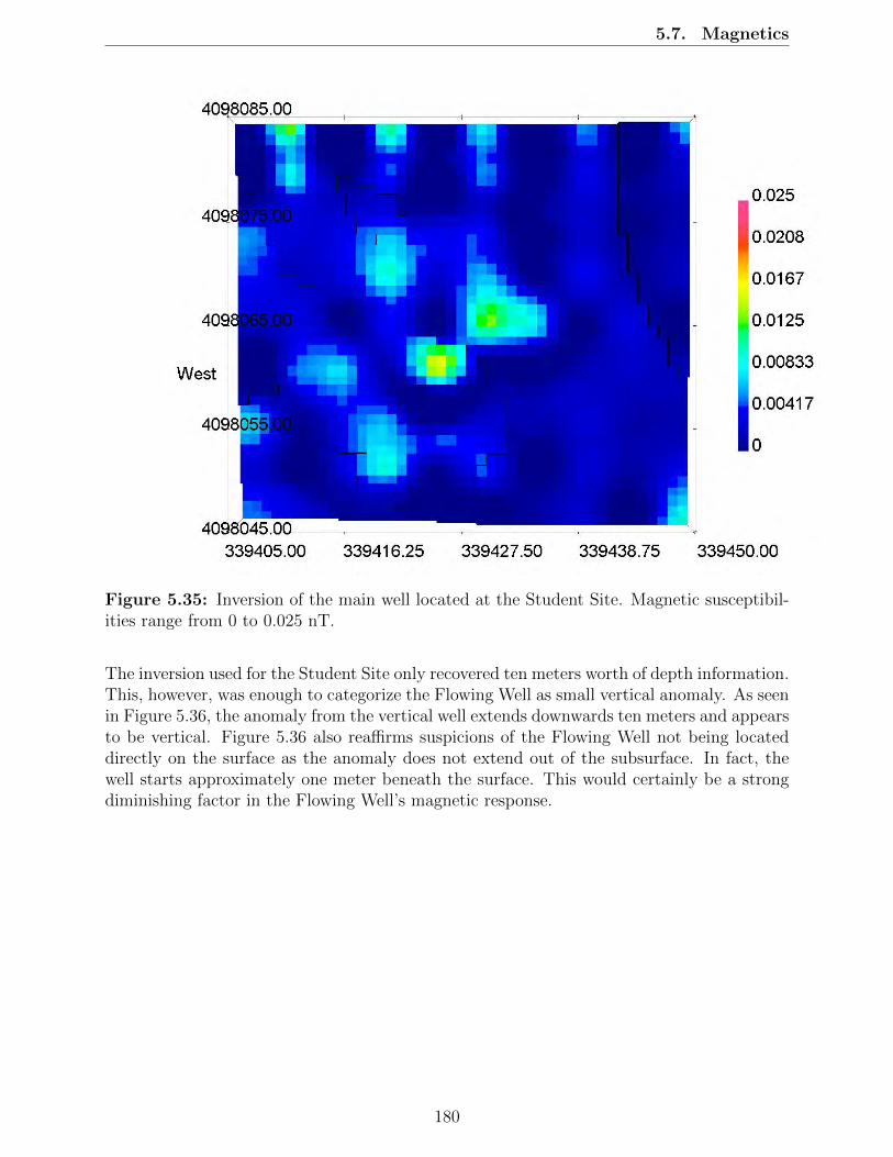
5.7. Magnetics
Figure 5.35: Inversion of the main well located at the Student Site. Magnetic susceptibil-ities range from 0 to 0.025 nT.
The inversion used for the Student Site only recovered ten meters worth of depth information.This, however, was enough to categorize the Flowing Well as small vertical anomaly. As seenin Figure 5.36, the anomaly from the vertical well extends downwards ten meters and appearsto be vertical. Figure 5.36 also reaffirms suspicions of the Flowing Well not being locateddirectly on the surface as the anomaly does not extend out of the subsurface. In fact, thewell starts approximately one meter beneath the surface. This would certainly be a strongdiminishing factor in the Flowing Well’s magnetic response.
180

5.7. Magnetics
Figure 5.36: Cross section of the inversion of the main well located at the Student Siteshowing the Flowing Well anomaly. Magnetic susceptibilities range from 0 to 0.025 nT.
5.7.5 Sources of Error/Uncertainty
A large source of error in this data set is the other surveys going on at the Student Site.The self-potential electrical survey was taking measurements on the grid at the time of thismagnetic survey and came close to the magnetometer twice, at line 7 and at line 9. Anothersource of error is the large culvert in the area. On the southeast side of the grid, there wasa large culvert with a diameter of around two meters. This skewed the magnetic data andaffected many of the points in the immediate area of the culvert. As stated in the processingsection, the largest spikes caused by the culvert were removed, but the majority of the noisecaused by the culvert stayed in the data set.
5.7.6 Conclusion
The inversions used for the Student Site produced acceptable results with reliable suscepti-bility and location. With more time these inversions could have been perfected by changingthe mesh in different ways. The resolution could have been increased in the Easting andNorthing directions over the anomalies to better pinpoint their location. The vertical stretch-ing could have also been increased to try to better understand the depths of the two wells.However, the inversions that were completed are still very useful. From these inversions wewere able to see the high susceptibility of the metal objects at the Student Site. This canbe used for future reference to know that when a susceptibility near 0.5 or above is seen,it is most likely a man made metal object. Our inversions also helped us understand thatthe Flowing Well is deeper and more corroded than the Secondary Well, which can be seenby the decreased magnetic response. This data can also be used with Self-Potential to helpunderstand the anomalies that are seen with that method. For example, the magnetics datashows that the Self-Potential data is not the result of a man-made anomaly outside of theculvert, power lines, and two wells.
181

5.8. Student Site Integration
5.8 Student Site Integration
Our goal at the student site was to design a survey as a class. This area had two buried wellcasings that provided good targets for electrical methods. Along with the results shown ineach of the individual method’s sections, the DC, magnetics, and EM taken at the studentsite can be integrated together to provide a better understanding of the sub surface near themain Flowing Well.
Figure 5.37: Field picture of the Flowing Well.
The Flowing Well has a mixture of water and oil bubbling up from the subsurface, whichcan be seen in Figure 5.37. Due to the high conductivity of rock saturated with water, DCand EM were both used to understand where the water was coming from, and due to themetallic nature of the well casing, magnetics was used to map the depth of the casing.
182

5.8. Student Site Integration
Figure 5.38: From left to right, DC, Magnetics, and EM taken directly over the FlowingWell.
Figure 5.38 shows images from each of the three methods used taken in the same locations.The GPS location of the Flowing Well is highlighted in red. Both DC and EM show a col-umn of increased conductivity at the location of the well. Since both of the methods showit, we can conclude that the data is correct, and that there actually is a column of increasedconductivity down to a depth of about 140 meters. The DC data only goes to about 20meters deep, but it allows us to conclude that the column of increased data in the EM is noterror in the data. It is possible that the well is deeper than 140 meters, but the EM dataonly shows the increased conductivity to that depth. While the magnetics can not showincreased conductivity, it does show the magnetic well casing. It can be seen that the casingstarts about one meter below the surface and is about ten meters long.
Combining these three methods allows to fully understand what is going on at the FlowingWell. The well casing was left in the borehole and spans only the very top of the hole.The water at the surface is coming up through the oil well shaft which can be seen by theincreased conductivity in a vertical line below the well. The oil that is mixed with the wateris remnants from the drilling the originally took place. The data for the Secondary Well isnot as conclusive as the data over the Flowing Welll because it was on the very edge of oursurvey grid. However, due to its close proximity, we can assume a very similar situatuionis happening. There is a borehole with a buried well casing at the top, and the bore holeallows water to come up to the surface.
The survey done at the student site showed that electrical methods are useful for locat-ing wells and buried well casings. This is useful because buried well casings can corrodeand pollute water, or damage drill bits if new wells are being drilled in the same area. Thesignature that would be expected for a retired well like Flowing Well or the Secondary Wellis a compact vertical feature with a high magnetic susceptibility followed by a large columnof increased conductivity.
183

CHAPTER 6
RECOMMENDATIONS
6.1 Suggestions for Future Work
Figure 6.1: Map of recommendations for future surveys.
The geophysical surveys that were carried out during this field camp provided valuable in-formation in order to characterize the structure of the subsurface below our line and providehypotheses of the fluid flow of the area. However, to continue characterizing the full geother-mal picture in Archuleta county, more surveys would need to be conducted in the area.We suggest additional data collection that would greatly augment our understanding of theregional geothermal system.
184

6.1. Suggestions for Future Work
• Survey Line between Pagosa Springs and Chromo: We recommend a surveyline consisting of the methods used in this field camp to be conducted to the northwestof our 2014 line. This line would be between Pagosa Springs and Chromo, and shouldideally be perpendicular to the anticline (Figure 6.1). The data collected from such aline would help image the lateral extent of the reverse fault we discovered on the 2014line. If the area is similarly faulted and fractured, the hypothesis that the water flowpath is routed through Pagosa Springs would be further supported.
• Longer seismic line: If additional surveys are to be done to the north, it is crucialthat Deep Seismic data be collected farther east than it was on our line. This willclear up the structure of the area to the east of our major reverse fault and answerwhether another reverse fault exists, as our Gravity and MT interpretations suggest.An understanding of the eastward faulting structure would give insight onto the extentof the geothermal system and whether geothermal resources south of Pagosa Springsare viable.
• Heat analysis: An investigation into the thermal gradient between Pagosa Springsand Chromo would give insight into the source mechanism of the geothermal system inthe entire region. The reason why the hot water in Chromo is significantly cooler thanin Pagosa Springs is still relatively unknown. Heat information, especially between thetowns of Pagosa Springs and Chromo would be valuable for exploring this question.
• Geochemical analysis: Geochemical analysis could tell us if the water is volcanicin origin. If the water is not volcanic in origin, the hypothesis of water flow throughfractured crystalline basement is strengthened due to the depths needed to heat thewater to geothermal temperatures purely by the Earth’s natural geothermal gradient.If the water is volcanic, additional geophysical techniques would be needed to determinethe exact flow path of the water to the Chromo region.
• Rock physics: Having definite values of the rock properties of the area would improvenearly every model made by each method including: gravity model with appropriatedensities, magnetics model with known magnetic susceptibilities, and velocity modelused for Deep Seismic processing. Methods which use inversion, such as DC, EM, andMagnetics, benefit from having known rock properties to guide the inversion process.While general rock properties can be researched, their accuracy compared to precisefield measurements on location is limited.
We put forth the conclusion that enough questions regarding the larger regional geothermalpicture exist for another field camp to return to Archuleta County. While additional localizedsurveys along our survey line could improve our data quality, exploring the larger story andconnections in between Pagosa Springs and Chromo is the most valuable use of money andtime.
185

CHAPTER 7
CONCLUSION
We succeeded in achieving both of our major goals for our 2014 Field Camp. Data collectionduring our two weeks in the field went smoothly and every student had the opportunity towork with each method. Proper field safety procedures were maintained and the quality ofacquisition is evident in the quality of the data we processed back in Golden. Additionally,our geophysical investigation in Chromo uncovered significant new geologic structures thatassist in explaining the geothermal fluid flow in the region.
Our seismic data strongly indicates the presence of a large thrust fault with 700-1000 metersof throw. This data is supported by our magnetotellurics, gravity, and geologic data. Wehave developed a geologic interpretation based on historical tectonic regimes that recon-structs the structure evident in our geophysical data. Our near surface methods as well asour seismic data suggest the presence of of normal faulted fracture zone beneath the StinkingSprings that could act as a conduit for water rising along the fault to express itself at thesurface. The conductivity values shown in our EM and DC data are adequate to supportfluid flow in the fracture zone.
We also connected our local structure to the larger setting, arguing for the flow of geothermalwater from the source location through Pagosa Springs to Chromo. The heavily fracturedcrystalline basement is likely the conduit between these two locations, although the DakotaSandstone is a viable layer of transport as well. Both explanations are plausible knowingbackground information about geothermal systems.
Our student site was chosen in Crowley Ranch. We designed a grid around two old oilwells with existing casings left in the ground in order to see if our near-surface geophysicaltechniques could characterize the extent of the wells and their corrosion. Our methods weresuccessful in locating the wells at depth, although large sources of cultural noise limited ourability to fully characterize the wells. However, the methodology was shown to be successfuland has potential applications at other similar sites.
We recommend future work be done in between Pagosa Springs and Chromo to evaluatethe regional setting and evaluate the temperature drop between the geothermal systems inthe two regions. Before attempting to use the hot water in Chromo for geothermal resources,additional characterization is needed. Our 2014 survey data will be an indispensable resourceto additional crews investigating the region, as the structures we have located are both newdiscoveries, and sensibly related to the Chromo geothermal system.
186

CHAPTER 8
APPENDIX
8.1 Geology
8.1.1 Well Log Information from COGCC [1]
Figure 8.1: Location of well logs used from COGCC
187

8.1. Geology
Table 8.1: OSTERHOUDT CROWLEY No. 1-7
Geologic layer Depth to top (m)Mesa Verde 142Mancos 227Greenhorn 808Graneros 822
Table 8.2: SHAHAN No. 1
Geologic layer Depth to top (m)Mancos 367Dakota 715
Table 8.3: AUSTRA-TEX SHAHAN No. 1
Geologic layer Depth to top (m)Greenhorn 722Dakota 753
Table 8.4: PC CROWLEY Heirs No. 1
Geologic layer Depth to top (m)Mesa Verde 126Mancos 221Greenhorn 789Graneros 803
Table 8.5: BAXSTROM No. 1
Geologic layer Depth to top (m)Greenhorn 593Dakota 647
Table 8.6: RUTH OSTERMAN No. 1
Geologic layer Depth to top (m)Greenhorn 564Dakota 613Morrison 680
188

8.1. Geology
Table 8.7: BROOKES No. 1
Geologic layer Depth to top (m)Mancos 396
Table 8.8: CHROMO FEDERAL No. 1
Geologic layer Depth to top (m)Greenhorn 154Graneros 164Dakota 212Morrison 296
Table 8.9: BRAMWELL No. 4
Geologic layer Depth to top (m)Greenhorn 151Graneros 158Dakota 213Morrison 296
189

8.2. Surveying
8.2 Surveying
8.2.1 Equipment Set Up for Differential GPS
Components of the differential GPS include the base station and the rover. The computerswithin these components are connected via blue tooth for Real Time Kinematics corrections,or they are connected after the survey for Post Processing Kinematics.
The first step in setting up the base station is choosing the location. The base stationshould be located in a region that is accessible and has no large obstructions that wouldprohibit connection to the rover. A region without trees on top of a hill is ideal. Next,a tripod to hold the receiver antenna is set up. The tripod must be leveled and orientednorth in order to have the most accurate location reading. The receiver antenna must thenbe connected to power and a radio. Next, a tripod to hold the transmitter antenna is setup. This tripod does not need to be leveled or oriented because its precise location is notnecessary. Next, the rover is set up. The rover is the instrument that we use at our surveylocations to make the GPS measurements. To set up the rover, an antenna is attached to theend of a pole and a computer is attached to the midpoint on the pole. Finally, we establisha connection between the rover and the base station. We used Real Time Kinematics GPSsurveys for our main line and for the student site in order to avoid post processing.
The rover component of the differential GPS is attached to a pole approximately two meterslong, and held vertically and level. The rover is connected via blue tooth to the base stationand makes real time corrections. To make measurements with the rover, stand at the pointof observation with the rover pole vertically upright and level (for more accuracy, use theleveling device on the pole). On the computer that is attached to the rover pole, check theflag number of the location and press enter.
Figure 8.2: Differential GPS base station set up [10]
190
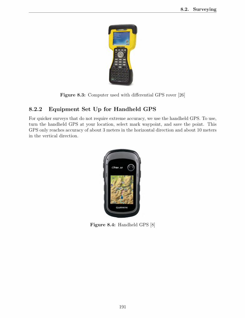
8.2. Surveying
Figure 8.3: Computer used with differential GPS rover [26]
8.2.2 Equipment Set Up for Handheld GPS
For quicker surveys that do not require extreme accuracy, we use the handheld GPS. To use,turn the handheld GPS at your location, select mark waypoint, and save the point. ThisGPS only reaches accuracy of about 3 meters in the horizontal direction and about 10 metersin the vertical direction.
Figure 8.4: Handheld GPS [8]
191

8.3. Gravity
8.3 Gravity
8.3.1 Control Parts for CG-5
1. Battery and battery charger, this provides power for the system.
2. Leveling base platform, this base is placed on the ground with the center over the pointyou would like to measure. The CG-5 is then placed on top of the platform.
3. Leveling adjustment screws and digital leveling display, from the menu of the CG-5,you are able to go into leveling mode. The screen then tells you which way to turn thescrews on the platform until the meter is leveled and you receive a smiley face.
4. Alpha-numeric key pad, the keypad on the CG-5 allows you to change the parametersof each measurement. You also use this to start a reading by pressing F5.
5. Digital graphics display, when a reading is taking place, the LED on the front willbe illuminated. When the light is off, the digital display will show a table with yourreading, standard deviation, and other parameters for the reading.
8.3.2 CG-5 Operations
1. Firmly plant the tripod into the ground in order to ensure the CG-5 will not settleinto the ground while taking measurements. Proceed to place the gravimeter onto thetripod and level the stand by turning the knobs; the CG-5 will display a happy facewhen the machine is level. A good strategy to level it is to fix the x and y planes beforeattempting to level the tripod in the z direction.
2. Once the machine is level, follow the prompts from the machine to set the surveyparameters. Use the keypad and the digitally displayed labels to the left to specifyconstraints.
3. Press F5 (the record command) to begin a reading. After giving the command, theoperator has about 5 seconds (depending on how long you set the delay) to vacate thearea, leaving at least 3 meters between the recorder and the machine. A blue lightshines to signal the recording has begun; when the light turns off, it is safe to approachthe instrument.
4. To be safe, write down the standard deviation, the gravity measurement, and the time.If the standard deviation is under .2, the measurement is good enough to keep. If all ofthe measurements have large standard deviations, repeat step 3. Press F5 to internallyrecord the data into the CG-5.
5. Navigate to the main screen. If that was the last measurement for the day, power themeter off and place it back into the carry case. If not, repeat steps 1-4 until satisfiedwith data collection.
6. A reading is taken at a base station for the first and last measurements of the day toaccount for drift.
192

8.4. Magnetics
8.4 Magnetics
8.4.1 Proton Precession Magnetometer
The proton precession magnetometer is used as a base station in the magnetic surveys.The base station is set up in an area away from noise interferences (such as metal fences,automobiles, etc.) and remained in this location for the entire day of surveying. Theprecession magnetometer only measured the total field strength, not the field direction.The use of this stationary magnetometer was to correct for diurnal variations.
8.4.2 Cesium Magnetometer
Two cesium magnetometers were used in vertical orientation with a G-858 MagMapperrecording system. With the vertical orientation, the bottom sensor provided a more detailedbut nosier data set, and the top sensor provided a less detailed, but less noisy dataset. Thetwo sensors were also used to calculate a vertical gradient. The cesium magnetometers wereused for data collection on both the main line and the student site. These magnetometersonly measured the total magnetic field and not the direction, similar to the proton precessionmagnetometer. the G-858 is capable of measuring continuously or at discreet points. Forboth the main line and the student site, the discrete mode was used.
Figure 8.5: Cesium Magnetometer in vertical orientation.
8.4.3 Operations
• Proton Precession Magnetometer
1. The magnetometer should be taken far away from all sources of noise (power lines,other surveys etc.).
2. Set the clock by pressing 2 (Auto), then 5 (Time), then 0 (Shift). Enter theGorean date and military time.
193
8.4. Magnetics
3. Set to Auto Store by pressing 2 (Auto), then 8 (Store), then Enter.
4. Set to Auto Record by pressing 2 (Auto), then 0 (Shift). Next, enter the recordingtime in seconds (we used 60s for our surveys).
5. At the end of the day, stop recording by pressing 2 (Auto), then Clear.
6. Download the data by plugging into computer and using the MagMap2000 importfeature. Follow the on-screen directions.
• Cesium Magnetometer
1. Connect cesium magnetometer cables to G-858.
2. Power on G-858. Test can be performed by going to System Setup → Magne-tometer Test.
3. Select Simple Survey.
– Pick file 1-5.
– Select continuous or discreet (discreet was used for our surveys).
– Set cycle time to 1.0 seconds.
4. Hit mark as the magnetometers cross the survey point.
5. Download the data by connecting to computer, selecting PC Controlled Transferon the G-858, and following the on-screen instructions from MagMap2000.
8.4.4 Smoothing Code
% MATLAB code: expo_smoothing.m
function [ smoothed_data ] = expo_smoothing(fdata, a )
x = fdata;
b = 1.0-a;
sx = 1.0;
sy = a;
yi = 0.0;
yi = sy*yi+sx*x(1);
y(1) = yi;
for i=2:length(fdata)-1
yi = a*yi+b*x(i);
y(i) = yi;
end
sx = sx/(1.0+a);
sy = sy/(1.0+a);
y(length(fdata)-1) = yi;
yi = sy*yi+sx*x(length(fdata)-1);
for i=length(fdata)-2:-1:1
yi = a*yi+b*y(i);
y(i) = yi;
end
smoothed_data = y;
194

8.4. Magnetics
% Clean your plate
clear all;
close all;
clc;
t=importdata(’MergedData.DAT’);
MergedData=t.data;
DeMergedData=MergedData;
for i=1:901
if MergedData(i,6) > 500 || MergedData(i,6) <-500
DeMergedData(i,6)= 0;
DeMergedData(i,7)= 0;
DeMergedData(i,5)= 0;
end;
end;
figure;
plot(MergedData(:,6));
%Top Diurnal
figure;
plot(DeMergedData(:,6));
hold on;
xxx = expo_smoothing(DeMergedData(:,6),.932);
zzz = expo_smoothing(xxx,.9);
plot(xxx,’g’);
plot(zzz,’r’);
% Bottom Diurnal
figure;
plot(DeMergedData(:,7));
hold on;
yyy = expo_smoothing(DeMergedData(:,7),.932);
www = expo_smoothing(yyy,.9);
plot(xxx,’g’);
plot(zzz,’r’);
195

8.4. Magnetics
%Vertical Gradient
figure;
plot(DeMergedData(:,5));
hold on;
aaa = expo_smoothing(DeMergedData(:,5),.932);
bbb = expo_smoothing(aaa,.9);
plot(aaa,’g’);
plot(bbb,’r’);
196

8.5. Self-Potential
8.5 Self-Potential
Signals at the ground surface can be generated by the corrosion of an ore body and the re-sulting distribution of redox potential. This phenomenon is described as a geobattery model.In this model, electrons found within the ore body have high mobility, but are not found inthe surrounding rock. The ore body can serve as a direct source of electrons by means ofoxidation and reduction, or merely as a conductor for the transfer of electrons throughoutthe subsurface. Far away from the ore body, the concentration of oxygen decreases withdepth, meaning at this distance the redox potential primarily depends on depth. Closer tothe body, the redox potential is influenced by anodic and cathodic reactions that exist dueto the corrosion of the body. This possibly provides a source of electrons and results in therelease of solubles that can interact with the oxygen present underground in the vicinity ofthe body. The variable distribution of this redox potential in itself is a mechanism drivingthe flow of current, since the gradient of the chemical potential of the electrons is one originof electrical current density, which is the source of self-potential signals. This geobatterymodel has been refined multiple times, resulting in both the Butler-Volmer model, whichaccounts for losses of electrical potential between the electron donors, acceptors, and themetallic body, as well as a biotic model in which bacterial biofilms are catalysts in electrontransfer between donors and acceptors. However, in any case, the underlying principle re-mains: the redox potential distribution present in the vicinity of the ore body (near and far)serves as a driving force for electrical current density, providing a source for self-potentialsignal.
Groundwater flow also provides a source for self-potential signals. As previously mentioned,water carrying excess charge produces a natural current. An electrical double layer foundat the pore-water/mineral interface of a grain is responsible for this charge found in thesubsurface (Figure 8.6). Chemical interactions between the surface sites and the pore waterresult in a mineral surface charge. When, for instance, silica comes in contact with water,it loses a proton and generates negative surface sites. Consequentially, the mineral surfacebecomes charged. This charge on the surface attracts counterions, which are positive in thecase of silica, and repels co-ions, or ions of the same charge. This results in what is calleda diffuse layer, a layer depleted of co-ions and rich in counterions, seen on the outside ofthe silica grain pictured in Figure 8.6. The other layer, the Stern layer, is found betweenthe mineral surface and the inner plane of the diffuse layer, as seen in Figure 8.6, and isformed by ions directly sorbing on the mineral surface. In this electrochemical system, thesetwo layers both possess an excess conductivity, combining to form an electrical double layeraround the insulating grain.
197

8.5. Self-Potential
Figure 8.6: Sketch of the electrical double layer comprised of the diffuse and Stern layersat pore-water/mineral interface, coating a grain of silica [39]
The existence of this double layer means that the pore water is non-neutral: when it flows,the drag of these excess charges in the diffuse layer generates an electrical current, called thestreaming current, as seen in Figure 8.7. This currnet makes self-potential measurementspossible. Secondly, this double layer explains the chargeability of porous materials in thatthere is a surplus of electrical conductivity near the pore-water/mineral interface.
198

8.5. Self-Potential
Figure 8.7: Flow of excess charge in a mineral grain with an electrical double layer. FigureCourtesy of Dr. Andre Revil.
Another source of self-potential signals is called the diffusion current, and can be attributedto the concentration gradients of ions and electrons, or charge carriers, present in the porewater of an insulated mineral grain. The diffusion of ionic charge carriers governs this cur-rent; differences in mobility of the cations and anions present in the pore water (Na+ andCl- in Figure 8.7) provide a source for current that is in turn driven by the gradient of thechemical potential of these ions.
199

8.6. DC Resistivity
8.6 DC Resistivity
8.6.1 Poisson Equation for Electric Field
In an electric field, the positive charge carriers move in the same direction as the electric field,while the negative charge carriers move in the opposite direction. The movement of chargesis called a current, and the flow per cross-sectional area is the flux. Electrical conduction,the generation of an electric field from a flux of current, is governed by Ohm’s Law, relatingthe current density (j in A m -2) to the electrical field (E in V/m) by the conductivity, orease by which current is able to flow through the ground:
j = σ0E (8.1)
Ohm’s Law is equivalent to that described in the self-potential method, except that in thiscase there is no source current density incorporated, since DC resistivity is an active methodin which a known amount of current is imposed. The electrical field resulting from electricalconduction can be decomposed in terms of its potential (in Volts), represented by ψ:
E = −∇ψ (8.2)
The gradient of the current density is equal to a volumetric charge source or sink term.Outside the areas where current is being injected or received, this volumetric term goes tozero, assuming there is no storage of electrical charges within the porous material givingoff a source current density, and that the current being injected into the ground must alsoleave this control volume. These conditions, equivalent to those outlined in the self-potentialmethod, result in the following continuity equation, where j represents the current density:
∇ · j = 0 (8.3)
As was the case with self-potential, inserting the equation for current density in terms of theelectric field, as well as the equation for the electric field in terms of potential results in thePoisson equation:
∇ · σ0∇ψ = 0 (8.4)
8.6.2 Heterogeneous Earth Model Theory
Resistance is obtained using Ohms law in the form of voltage, current, and resistance:
4ψ = U = IR (8.5)
where U is difference in potential, or voltage, and R is resistance of the rock unit. Thisrelationship can be rearranged as follows:
R =U
I=4ψI
(8.6)
Resistance is equal to the observed voltage drop over the given injected current, both of
200

8.6. DC Resistivity
which are known or measurable quantities in this experiment. Thus, resistance itself is anobservable quantity that can relate current to voltage.
Assuming the earth beneath the acquisition is a homogeneous, semi-infinite half-space withuniform resistivity, the Poisson equation (8.4) mentioned previously simplifies to theLaplacian equation since the ground in this case is a piecewise, homogeneous domain,and the potential at point P can be measured using the following relationship:
ψ(P ) =Iρ
2π(
1
ra− 1
rb) (8.7)
where ra and rb are located at point P and represent the distances to electrodes A and B,respectively, I is the injected current, and ρ is the uniform resistivity of the halfspace.
By using Equation 8.7 and inputting the locations of the potential electrodes M and N,as well as applying the superposition principle, the following equation is obtained for thedrop in potential, or voltage, between M and N for a homogenous earth with constant resis-tivity:
U = 4ψ = ψ(M)− ψ(N) =Iρ
g= IR (8.8)
where g is the geometrical factor for a given four-electrode array, relating measured resistancefor a given current to resistivity:
1
g= 2π(
1
AM− 1
BM− 1
AN+
1
BN) (8.9)
For a heterogeneous earth model, an apparent resistivity (ρa), or a weighted average ofsubsurface resistivity, can be obtained using the measured resistance (8.6) and the knowngeometric factor (8.9):
ρa = Rg (8.10)
Resulting apparent resistivity data can then be inverted to obtain true subsurface resistivity.
8.6.3 Detail: Main Line Survey Design
8 reels of takeout cables were used in total during each acquisition done on the main line.4 reels on each side of the midpoint were used, with two extra reels to cut down on timebetween acquisitions. Each reel connected to 8 electrodes, for a total of 32 electrodes oneach side of the midpoint, and 64 electrodes in total. This survey length resulted in 472points in the raw pseudosection for the initial acquisition, seeing roughly 220 meters into theground. 40 additional points were incorporated with each ”up”, or each time the midpointwas shifted West by two reels.
201

8.6. DC Resistivity
8.6.4 Student Site: Additional DC Images
Figure 8.8: Aerial image of DC lines 3 and 8 bisecting the Flowing Well site
202

8.6. DC Resistivity
Figure 8.9: Aerial image of DC lines 3 and 8 bisecting the Flowing Well site
203

8.6. DC Resistivity
Figure 8.10: Surface map of 3D interpolation of DC Resistivity data at Flowing Wellstudent site
204
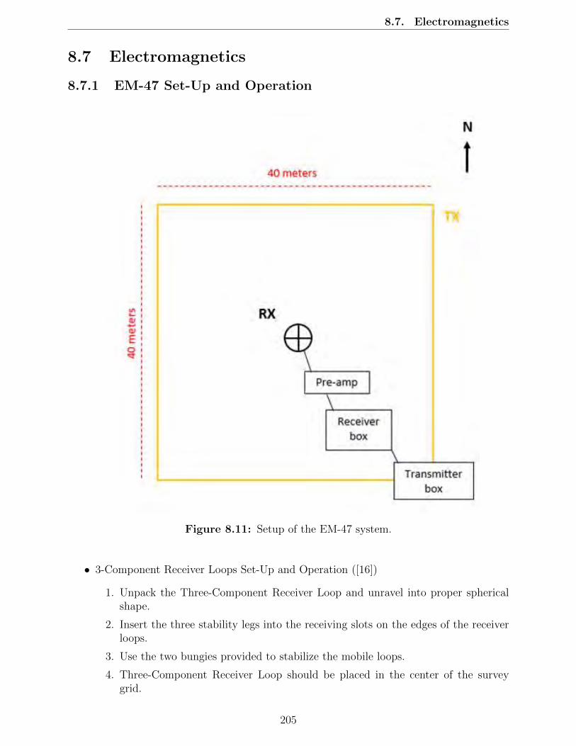
8.7. Electromagnetics
8.7 Electromagnetics
8.7.1 EM-47 Set-Up and Operation
Figure 8.11: Setup of the EM-47 system.
• 3-Component Receiver Loops Set-Up and Operation ([16])
1. Unpack the Three-Component Receiver Loop and unravel into proper sphericalshape.
2. Insert the three stability legs into the receiving slots on the edges of the receiverloops.
3. Use the two bungies provided to stabilize the mobile loops.
4. Three-Component Receiver Loop should be placed in the center of the surveygrid.
205

8.7. Electromagnetics
5. Orient the receiver loops with survey. This can be done by using the compasslocated on the receiver loop. Standard operating procedure is to align the redarrow of the compass with the desired direction.
6. Level the receiver loops via the bubble located near one leg. This can be doneby releasing and adjusting each leg at a time until the bubble is located in thecenter.
• Protem Receiver
1. Turn the receiver on by inserting battery and switching the unit to ON. Thisswitch is located on the interior panel of the receiver.
2. When the receiver has powered up, a a prompt will appear stating whether to use20 or 30 gates. Select preference by using the arrow keys and the enter buttonlocated on the interior panel.
3. To connect Protem-D receiver with current loop a pre-amp is provided. The pre-amp will have one end compatible with the back of the Protem-D receiver andone multi-end associated with the receiver loops. The multi-end portion of thepre-amp will be labeled either X,Y, or Z and will correspond with similar labelson the receiver loops. Simply plug in both ends.
4. A cable referred to as the reference cable should be plugged into the Protem-Dreceiver. This will be inserted into the correspond two-prong receiver slot. Theorientation does not necessarily matter, but should be kept consistent.
5. To ensure unit is functional after current loop is constructed, current is flowing,and all cables are connected, there is a test function on the main menu representedby T. Select with arrow keys and enter.
6. To adjust survey parameters, the main menu will have an option represented withA meaning adjust. In this menu, settings such as integration time and frequencycan be adjusted. To change options simply navigate the screen with arrows andthe enter key. To leave this menu simply hit the button labeled MM for mainmenu.
7. To measure after desired settings are in place, simply press the M on the mainmenu for measure. This will display a screen with an initial reading. Press enterone more time to record.
• Protem 47 Transmitter [16]
1. Connect to Protem-D receiver via reference cable. Plug one end into the socketlocated on the front of the transmitter.
2. Connect to battery via port on front of transmitter.
3. Construct current loop. If the desired grid is rectangular, corners must be per-fectly perpendicular. Again, this can be accomplished with use of a compass. Theeasiest way to do this is have one person stand in the center of the grid directinga person with a stake to the proper angle at the proper distance. A third personshould align themselves with the other two people at the correct distance. Repeatfor other two corners. Note: grid and receiver loops must be oriented in the samedirection.
206

8.7. Electromagnetics
4. Using desired current cable, run the cable around the edges of the grid and connecteach end to front of transmitter.
5. Turn on the machine using labeled power switch located on the front of the trans-mitter underneath the LCD display screen.
6. Adjust loop size by using knob located on the front of receiver.
7. Adjust current using the dial labeled CURRENT located on the top right of thefront face of the transmitter.
8.7.2 Conductivity Derivation
1
σ=
[Iµ
52o a2
20π12∂Bz
∂tt52
] 23
(8.11)
The variables are as follows:
• σ is conductivity
• I is current
• t is time
• µo is permeability of free space
• a is area of the loop
• ∂Bz
∂tis the time derivative of the magnetic field
∂Bz
∂tcan be further defined as:
∂Bz
∂t= − I
σa3
[3erf(θa)− 2√
πθa(3 + 2θ2a2
)e−θ
2a2
](8.12)
where θ =√
µoσ4t
and erf(x) is the error function, erf(x) = 2√π
∫ x0e−t
2dt.
8.7.3 Survey Parameters in Chromo, CO
• Survey was aligned north-south.
• The TX loop size was set to 40m x 40m.
• Only field information in the Z direction was collected due to time constraints.
• Number of recordings per frequency was set to three.
8.7.4 Survey Parameters at Student Site
• Survey was aligned to coincide with the student site survey grid.
• The TX loop size was set to 80m x 80m.
• Only field information in the Z direction was collected due to time constraints.
• Number of recordings per frequency was set to 1.
207

8.7. Electromagnetics
Table 8.10: Main Line Survey Parameters for Recording
Frequency (Hz) Integration Time, or RT (s) Current (A)285 30 2.575 60 3.030 120 3.0
Table 8.11: Student Site Survey Parameters for Recording
Frequency (Hz) Integration Time, or RT (s) Current (A)285 30 3.075 30 2.5
8.7.5 Time Gates for Frequencies Used
Frequency: 285Hz 75Hz 30HzGate Time(µs) Time(µs) Time(µs)
01 6.000 32.00 80.0002 7.625 38.50 96.2503 9.750 47.00 117.504 12.50 58.00 145.005 15.88 71.50 178.806 20.25 89.00 222.507 25.88 111.5 278.808 33.00 140.0 350.009 42.13 176.5 441.310 53.75 223.0 557.511 68.50 282.0 705.012 87.38 357.5 893.813 111.4 453.5 1134.14 151.7 576.0 1440.15 181.1 732.5 1831.16 231.0 932.0 2330.17 294.6 1187. 2966.18 375.9 1512. 3779.19 479.5 1926. 4815.20 661.6 2455. 6136.
Table 8.12: Protem Digital Reciever Recordings per Frequency
208
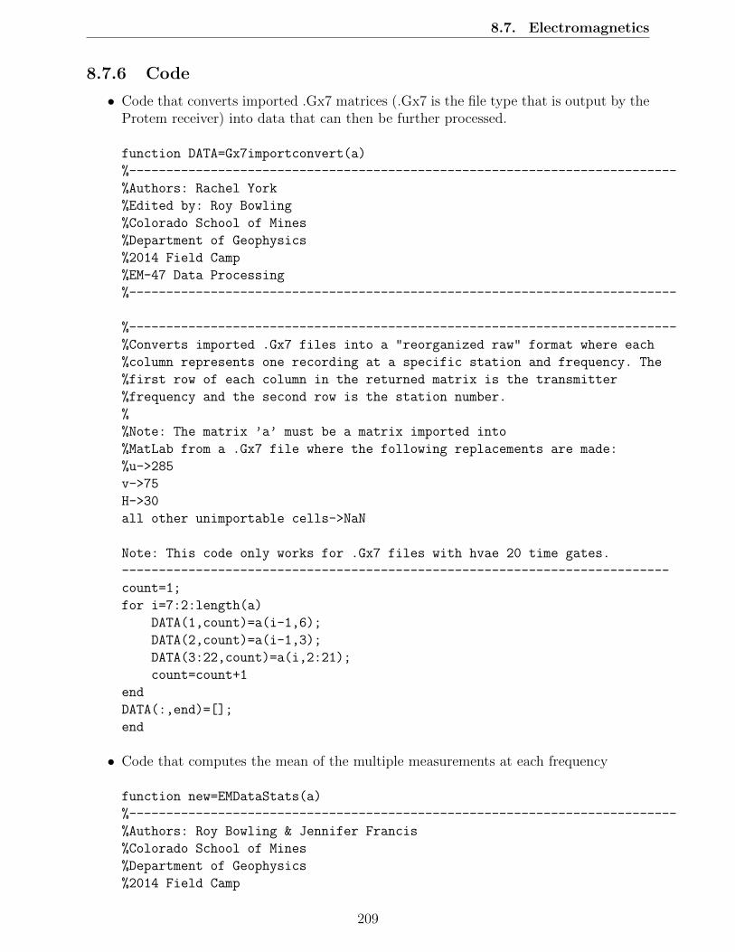
8.7. Electromagnetics
8.7.6 Code
• Code that converts imported .Gx7 matrices (.Gx7 is the file type that is output by theProtem receiver) into data that can then be further processed.
function DATA=Gx7importconvert(a)
%--------------------------------------------------------------------------
%Authors: Rachel York
%Edited by: Roy Bowling
%Colorado School of Mines
%Department of Geophysics
%2014 Field Camp
%EM-47 Data Processing
%--------------------------------------------------------------------------
%--------------------------------------------------------------------------
%Converts imported .Gx7 files into a "reorganized raw" format where each
%column represents one recording at a specific station and frequency. The
%first row of each column in the returned matrix is the transmitter
%frequency and the second row is the station number.
%
%Note: The matrix ’a’ must be a matrix imported into
%MatLab from a .Gx7 file where the following replacements are made:
%u->285
v->75
H->30
all other unimportable cells->NaN
Note: This code only works for .Gx7 files with hvae 20 time gates.
--------------------------------------------------------------------------
count=1;
for i=7:2:length(a)
DATA(1,count)=a(i-1,6);
DATA(2,count)=a(i-1,3);
DATA(3:22,count)=a(i,2:21);
count=count+1
end
DATA(:,end)=[];
end
• Code that computes the mean of the multiple measurements at each frequency
function new=EMDataStats(a)
%--------------------------------------------------------------------------
%Authors: Roy Bowling & Jennifer Francis
%Colorado School of Mines
%Department of Geophysics
%2014 Field Camp
209

8.7. Electromagnetics
%EM-47 Data Processing
%--------------------------------------------------------------------------
%--------------------------------------------------------------------------
%Averages the multiple readings at each frequency, DOES NOT REMOVE
%OUTLIERS, outliers must be removed by hand. Returns a matrix ’new’ where
%each column represents the average of multiple readings measured for each
%frequency at a specific station location. The first row of each colunm in
%the returned matrix is the transmiter frequecny and the second
%row is the station number. All other rows in each column represent
%averaged measurements in nV/m^2
%
%Note: This code will work for matrixed derived from either 20 or 30 time
%gates
%
%Note:the matrix ’a’ must be a matrix in the form outputed by
%Gx7importconvert.m
%--------------------------------------------------------------------------
new=0;
j=1;
i=1;
last=length(a(:,1));
while i~=(length(a(1,:))+1)
counter=1;
sum=a(1:last,i);
avg=0;
while(i~=length(a(1,:))&& a(1,i)==a(1,i+1) && a(2,i)==a(2,i+1))
counter=counter+1;
sum=sum+a(1:last,i+1);
i=i+1;
end
avg=sum/counter;
new(1:last,j)=avg;
i=i+1;
j=j+1;
end
end
• Code that takes the imported and averaged EM-47 data and converts it into nV permeter squared.
function new=Averagedtonvm2(a,gain)
%--------------------------------------------------------------------------
%Authors: Roy Bowling & Jennifer Francis
210

8.7. Electromagnetics
%Colorado School of Mines
%Department of Geophysics
%2014 Field Camp
%EM-47 Data Processing
%--------------------------------------------------------------------------
%--------------------------------------------------------------------------
%Converts an array exported by EMDataStats to values expressed in
%normalized nano-volts per meter squared. Taken into account is the pre
%selected gain of 51.2 the user selected gain, ’gain’ and the effective
%area if the 3D-1 receiver coil.
%--------------------------------------------------------------------------
lastcol=length(a(1,:))
lastrow=length(a(:,1))
new=zeros(lastcol,lastrow);
for i=1:1:lastcol
new(1,i)=a(1,i);
new(2,i)=a(2,i);
for j=3:1:lastrow
new(j,i)=((a(j,i)*(1e6))/((51.2)*(2^(gain))*(31.4)));
end
end
• Code that plots the voltage decay curve of voltage versus time for preliminary purposes
function DecayCurveploter(a)
%--------------------------------------------------------------------------
%Authors: Roy Bowling & Jennifer Francis
%Colorado School of Mines
%Department of Geophysics
%2014 Field Camp
%EM-47 Data Processing
%--------------------------------------------------------------------------
%--------------------------------------------------------------------------
% Function that takes an array a which must be one or more
% columns of an array outputed by Averagedtonvm2.m This code plots the
%measured voltage versus time.
%--------------------------------------------------------------------------
figure
for i=1:1:length(a(1,:))
Hz=a(1,i)
if Hz==285
t=[6.000
7.625
9.750
12.50
15.88
20.25
211

8.7. Electromagnetics
25.88
33.00
42.13
53.75
68.50
87.38
111.4
151.7
181.1
231.0
294.6
375.9
479.5
611.6];
V=a(3:end,i);
elseif Hz==75
t=[32.00
38.50
47.00
58.00
71.50
89.00
111.5
140.0
176.5
223.0
282.0
357.5
453.5
576.0
732.5
932.0
1187
1512
1926
2455];
V=a(3:end,i);
elseif Hz==30
t=[80.00
96.25
117.5
145.0
178.8
222.5
278.8
350.0
441.3
212

8.7. Electromagnetics
557.5
705.0
893.8
1134
1440
1831
2330
2966
3779
4815
6136];
V=a(3:end,i);
else
disp(’Error unrecognized frequency’);
end
%gates=1:1:20;
loglog(t,V,’LineWidth’,1);
hold on
end
%title(’Decay of Flux as a Function of Time May 18th’,’FontSize’,14,
’FontWeight’,’bold’)
xlabel(’ns’,’FontSize’,11,’FontWeight’,’bold’)
ylabel(’nV/m^2’,’FontSize’,11,’FontWeight’,’bold’)
set(gcf,’Color’,’white’)
set(gca,’FontSize’,8);
set(gca,’normal’);
• Code that interpolates and plots inverted EM-47 1D sounding data
function EMsectionPlotter(Length,Depth,Roh)
%--------------------------------------------------------------------------
%Authors: Roy Bowling & Jennifer Francis
%Colorado School of Mines
%Department of Geophysics
%2014 Field Camp
%EM-47 Data Processing
%--------------------------------------------------------------------------
%-------------------------------------------------------------------------
% This function takes three column vectors corresponding to horizontal
% locations, vertical locations, and resitivites respectively and creates a
% psuedo-2D interpolated cross section. The interpolation between points is
% linear because the data is scattered.
% NOTE: If extent of section is significantly larger than extent of true
% data points liner interpolation will produce considerable artifacts
%-------------------------------------------------------------------------
Depth=(-1)*Depth;
213

8.7. Electromagnetics
Int=scatteredInterpolant(Length,Depth,Roh);
d=input(’How deep will the depth scale go?:’);
a=input(’Length-wise the the data will be plotted from
(enter Easting/Northing Coordinate):’);
b=input(’Now enter the terminating Easting/Northing Coordinate:’);
sL=input(’Enter the Easting/Northing spacing:’);
sD=input(’Enter the depth spacing’);
[gL,gZ]=meshgrid(a:sL:b,0:sD:d);
Mesh=Int(gL,gZ);
%Mesh=griddata(Length,Depth,Roh,gL,gZ,’cubic’)
Title=input(’Enter the title of this plot:’,’s’);
Xlabel=input(’Enter the length axis label:’,’s’);
figure
contourf(gL,gZ,Mesh,30);
set(gca,’YDir’,’reverse’)
hold on
scatter(Length,Depth,35,’black’,’filled’);
set(gcf,’Color’,’white’);
set(gca,’XAxisLocation’,’top’);
title(Title,’FontSize’,20,’FontWeight’,’bold’);
ylabel(’Depth (m)’,’FontSize’,16,’FontWeight’,’bold’);
xlabel(Xlabel,’FontSize’,16,’FontWeight’,’bold’);
colormap(jet);
t = colorbar(’peer’,gca);
set(get(t,’ylabel’),’String’,’Ohm-m’,’FontSize’,16,’FontWeight’,’bold’);
214

8.8. Magnetotellurics
8.8 Magnetotellurics
8.8.1 Assumptions of MT Method
Simplifying assumptions are applied in MT surveys in order to study electromagnetic induc-tion in the Earth [43].
1. Maxwell’s electromagnetic equations are obeyed.
2. The Earth only dissipates or absorbs electromagnetic energy.
3. Fields are treated as conservative and analytic at a distance from their sources.
4. Natural electromagnetic source fields are being generated by large-scale ionosphericcurrent systems that are relatively far away, and can therefore be treated as uniform,plane-polarized electromagnetic waves impinging on the Earth at near-vertical inci-dence. This assumption may be violated in polar and equatorial regions.
5. No accumulation of free charges is expected to be sustained within a layered Earth. In amulti-dimensional Earth, charges can accumulate along discontinuities. This producesstatic shift.
6. Charge is conserved, and the Earth behaves as an ohmic conductor, obeying Equa-tion 8.13:
j = σE (8.13)
where j is total electric current density, σ is the conductivity of the sounding medium,and E is the electric field.
7. The electric displacement field is quasi-static for MT sounding periods. Therefore,time-varying displacement currents are negligible compared with time-varying conduc-tion current and therefore electromagnetic induction can be treated as solely a processof diffusion.
8. Any variations in the electrical permittivities and magnetic permeabilities of rocks areassumed negligible compared with variations in bulk rock conductivities.
8.8.2 Diffusion Equation
The vector identity (Equation 8.14) is applied after taking the curl of Faraday’s Law or ofthe Ampere-Maxwell Law in order to calculate a diffusion equation[43].
~∇×(~∇× F
)=(~∇ · ~∇ · F
)− ~∇2F (8.14)
If we assume the divergence of the electric field to be zero then we can derive the diffusionequation as Equation 8.15.
~∇2E = µoσ∂E
∂t(8.15)
215

8.8. Magnetotellurics
The electric field is assumed to have an initial amplitude at the surface and to oscillateharmonically, and the solution to the differential calculation is seen in Equation 8.16.
~∇2E = iωµ0σE (8.16)
The conductivity of air is near 0, and therefore insignificant attenuation of EM waves isexperienced between the ionosphere and the surface of the Earth.
8.8.3 Impedance Tensor
MT measures orthogonal components of natural magnetic and electric fields, which arerelated by the impedance tensor (Equation 8.17).
(ExEy
)=
(Zxx ZxyZyx Zyy
)
Bx
µ0
By
µ0
(8.17)
The impedance tensor is complex, meaning it has both magnitude and phase (Equation 8.17).
φij = tan−1ImZijReZij
(8.18)
Phase lag corresponds to the time necessary for EM waves to diffuse through the subsurface.Dimensionality information is also present in the impedance tensor. In a 1-D Earth, theoff-diagonal components are equal but opposite in sign, while the diagonal components areequal to zero (Equation 8.19).
Zxx = Zyy = 0 and Zxy = −Zyx (8.19)
In a 2-D Earth, the impedance tensor is the same as Equation 8.19 if one of the X and Ydirections is oriented along electromagnetic strike. Electromagnetic strike is the strike of theconductivity structure, which is often analogous to geologic strike. Zxx and Zyy are almostalways not equivalent to zero in practice, arising from 3-D induction and distortion.
The dimensionality of the impedance tensor is scale dependent. For shorter sounding peri-ods when the inductive scale length is significantly shorter than the smallest dimension ofthe anomalous body, the edges of the anomalous body are not sensed and the conductivitystructure appears 1-D. As sounding period increases and inductive scale length increases toencompass the edges of the anomalous body, the structure appears 2-D. An even furtherincrease in sounding period causes the inductive scale length to cover all edges of the anoma-lous body, and the conductivity structure appears 3-D. The impedance tensor is calculatedover 360 degrees using data in the xy direction as well as the yx direction. Examining theimpedance tensor for each frequency allows us to identify where the structure changes from1-D to 2-D or 3-D, which is useful for identifying the location of faults. 1-D structures willhave a small response in the xx direction approaching a point while the xy direction will beextremely circular and become increasingly more oblong and asymmetric as the subsurface
216

8.8. Magnetotellurics
becomes more 2-D and 3-D. Figure 8.12 shows a 1-D impedance tensor with some possible2-D structures[9].
Figure 8.12: 1-D impedance tensor with some 2-D features. Orange represents the xxdirection and blue represents the xy direction.
8.8.4 Apparent Resistivity and Impedance Phase
In an N-layered model, each layer has a conductivity σn, a diffusion equation, and a solutionto the electromagnetic diffusion equation yielding an electric and magnetic field in the formof Equation 8.20 and Equation 8.21 respectively[43]:
Exn (qn, ω) = E1neiω−qnz + E2ne
iω+qnz = an (qn, ω) e−qnz + bn (qn, ω) e+qnz (8.20)
Byn (qn, ω) =qniω
[an (qn, ω) e−qnz + bn (qn, ω) e+qnz] (8.21)
where qn =√iµ0σω but incorporates the conductivity of the Nth layer as well. Transfer
functions seen as Equation 8.22 and Equation 8.23 can be calculated for each MT sounding.
Cn (z) =Exn (z)
iωByn (z)and qn =
√iµ0σnω (8.22)
Cn (zn−1) =ane
−qnzn−1 + bneqnzn−1
qn(ane−qnzn−1 − bneqnzn−1)(8.23)
The transfer function can then be calculated at the top and bottom of each layer withinthe half space. A term for the ratio of an/bn is derived, and continuity conditions are thenapplied to yield Wait’s recursion formula (Equation 8.24). Wait’s recursion formula is usedto calculate apparent resistivity at the surface, which can be measured by the MT survey[43].
217

8.8. Magnetotellurics
Cn (zn−1) =1
qn
qnCn+1(zn) + tanh(qnln)
1 + qnCn+1(zn) tanh(qnln)(8.24)
Impedance phase is calculated using equation Equation 8.25.
φ1−D = tan−1Ex/By (8.25)
A homogeneous half space will have a phase of 45 degrees. If resistivity increases with depth,phase will decrease below 45 degrees, and if resistivity decreases with depth, phase increasesabove 45 degrees. For further information on phase and apparent resistivity calculations andtheory see the references [43].
8.8.5 Electromagnetic Skin Depth
Skin depth is calculated as Equation 8.26. Here we can see that lower frequencies willcorrespond to a larger skin depth. Small MT sounding periods corresponding to small skindepths should yield transfer functions that appear 1-D. As the sounding period increases,the transfer function will increase in dimensionality to the point where the skin depth ismuch larger than the anomaly dimensions. This creates a non-inductive response causing afrequency-independent distortion of the transfer function[43].
δ = 503√σf (8.26)
218

8.9. Ground Penetrating Radar
8.9 Ground Penetrating Radar
Listed below are some of the fundamental mathematical relations for electromagnetic wavesused in GPR surveying.
The velocity of electromagnetic wave in an insulator is given by Equation 8.27:
V =c√µ · ε (8.27)
where c is the velocity of light in vacuum 3x10ˆ8 m/s and ε is the relative electric permittivity.The wavelength of electromagnetic wave traveled in any material is given by Equation 8.28:
λ =c
f√ε
(8.28)
where λ is the wavelength of electromagnetic wave and f is the frequency of electromagneticwave.
219

8.10. Hammer Seismic
8.10 Hammer Seismic
8.10.1 Refraction
Processing Techniques
Several techniques can been applied in order to analyze and interpret refracted wave data.Each method provides a different degree of accuracy and has its own advantages and limi-tations.Three common methods are listed below:
1. A single subsurface interface
2. Two horizontal interfaces
3. Dipping interfaces
A Single Horizontal Interface
This method assumes that there is only one geologic boundary for the refraction to returnenergy to the surface. This refraction phenomena is based on Snell’s law, critical angle, andcritical refraction.
Figure 8.13: Diagram illustrating symbols used in derivation of time of travel for criticallyrefracted rays.
In Figure 8.13, we see that acoustic energy is created by hitting a metal plate on the groundwith a sledgehammer at point E and a geophone is planted at point G. A compressional wavetravels at velocity V1 and hits the interface of two different velocity layers, V1 and V2. Whenthe compressional wave hits the contact at the critical angle θic , it is refracted parallel to theinterphase with the velocity V2. Then, the wave propagates back to surface from point N to G.
220

8.10. Hammer Seismic
Figure 8.14: Generalized diagram illustrating ray paths in rock layers with one horizontaldiscontinuity. Time-distance relationships for both the direct and refracted rays are shownin the travel-time curve.
From Figure 8.13, we are able to calculate the velocity of each layer and the thickness of thetop layer (layer that has v1 velocity). The plot of time and distance can be utilized fromFigure 8.13. The velocity of the top layer (v1) and second layer (v2) can be calculated byusing Equation 8.29.
v =∆distance
∆time(8.29)
Additionally, we can determine the thickness from:
h1 =ti2
V2V1
(V 22 − V 2
1 )12
(8.30)
where h1 and v1 are the thickness and velocity of top layer, respectively.v2 is the velocity of bottom layer.ti is the intercept time from the time-distance plot for each shot.
Two Horizontal Interfaces
The configuration of this model is shown in Figure 8.15. This model is similar to previousone interface model due to the horizontal orientation of the layers. Thus, the velocity of
221
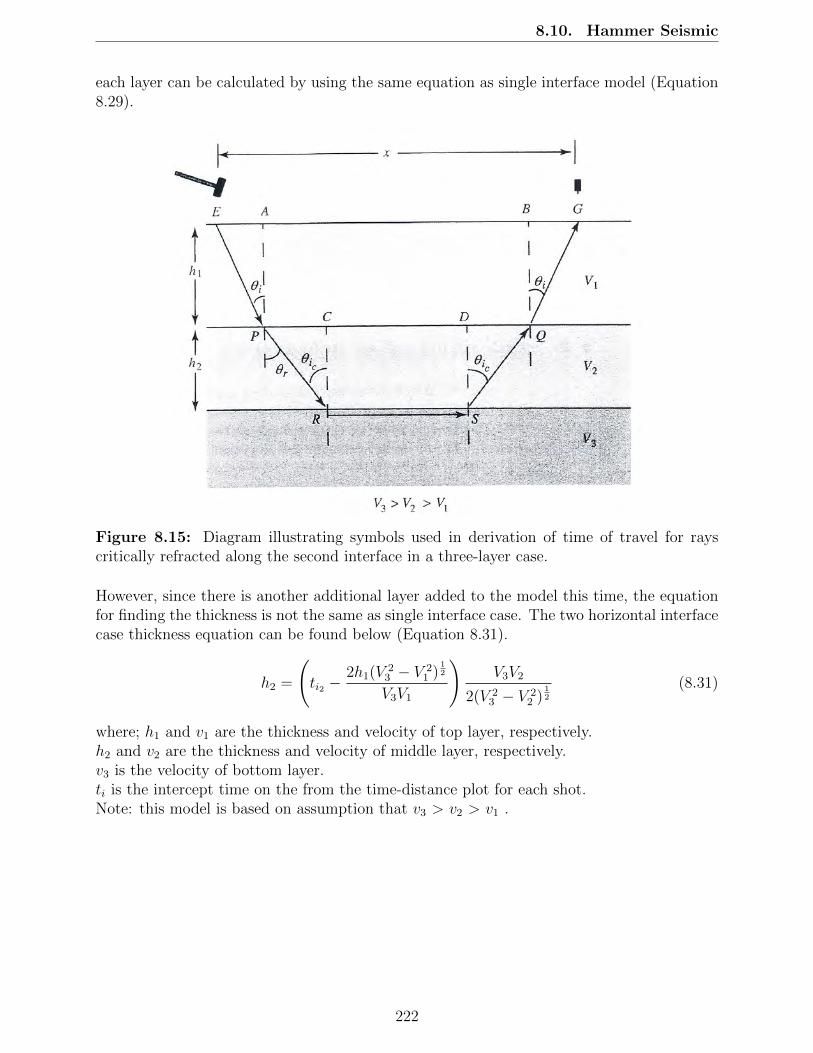
8.10. Hammer Seismic
each layer can be calculated by using the same equation as single interface model (Equation8.29).
Figure 8.15: Diagram illustrating symbols used in derivation of time of travel for rayscritically refracted along the second interface in a three-layer case.
However, since there is another additional layer added to the model this time, the equationfor finding the thickness is not the same as single interface case. The two horizontal interfacecase thickness equation can be found below (Equation 8.31).
h2 =
(ti2 −
2h1(V23 − V 2
1 )12
V3V1
)V3V2
2(V 23 − V 2
2 )12
(8.31)
where; h1 and v1 are the thickness and velocity of top layer, respectively.h2 and v2 are the thickness and velocity of middle layer, respectively.v3 is the velocity of bottom layer.ti is the intercept time on the from the time-distance plot for each shot.Note: this model is based on assumption that v3 > v2 > v1 .
222

8.10. Hammer Seismic
Figure 8.16: Generalized diagram illustrating ray paths in a subsurface model with twohorizontal interfaces. Time-distance relationships for the direct and two critically refractedrays are shown in the travel-time curve.
Dipping Interfaces
We previously discussed the model of horizontal interfaces for our reflection method. How-ever, anticlines, synclines, or other irregular structures can occur in the subsurface. Thesecannot be handled by a horizontal model. Thus, we need to construct the relationship fordipping interfaces to deal with real world situations.
To begin with, it is noteworthy to mention that the travel-time curve of the single dippinginterface, Figure 8.16, has a different shape when compared to the horizontal layers model,Figure 8.17. The time from forward and reverse shot points to a geophone at a given distanceare not equal. However, the reciprocal time must be equal. From Figure 8.17, we define mu
and md to be the slope of the straight line equation; y=mx+b.
slope = mu =1
V2R(8.32)
slope = md =1
V2F(8.33)
223
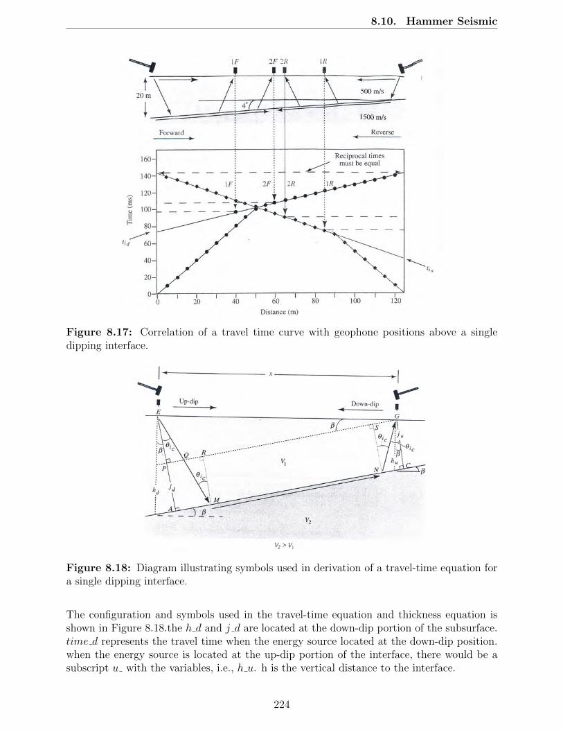
8.10. Hammer Seismic
Figure 8.17: Correlation of a travel time curve with geophone positions above a singledipping interface.
Figure 8.18: Diagram illustrating symbols used in derivation of a travel-time equation fora single dipping interface.
The configuration and symbols used in the travel-time equation and thickness equation isshown in Figure 8.18.the h d and j d are located at the down-dip portion of the subsurface.time d represents the travel time when the energy source located at the down-dip position.when the energy source is located at the up-dip portion of the interface, there would be asubscript u with the variables, i.e., h u. h is the vertical distance to the interface.
224

8.10. Hammer Seismic
The travel time equations when the energy source is located down-dip and up-dip are shownbelow.
Timed =2jd cos θic
V1+
x
V1sin (θic − β) (8.34)
Timeu =2ju cos θic
V1+
x
V1sin (θic − β) (8.35)
To find v 2 we have to know θ i c and solve this equation.
sin θic =V1V2
(8.36)
The θic and β can be calculated if we know the velocity v1 and the slope md and mu by usingthis set of equations.
θic =arcsin (V1md) + arcsin (V1mu)
2(8.37)
β =arcsin (V1mu)− arcsin (V1md)
2(8.38)
The intercept time of down-dip portion and up-dip portion can be calculated by
tid =2jd cos θic
V1(8.39)
The equations for thickness of both up-dip (ju, hu) and down-dip portion (jd hd) of thesubsurface structure are listed below.
jd =tidV1
2 cos θic(8.40)
ju =tiuV1
2 cos θic(8.41)
hd =jd
cos β(8.42)
hu =ju
cos β(8.43)
where; tid is the intercept time of down-dip portion. tiu is the intercept time of up-dipportion. v1 is the velocity of the top layer. the definition of all associated angle β , θic canbe found in Figure 8.18
225

8.11. Seismic: Survey Design
8.11 Seismic: Survey Design
When designing a Deep Seismic survey it is vital to take into account the geology of the areaand the topography. Certain parameters need to be decided on, such as source and receiverspacing, and whether or not the spread would be a split spread or an off end spread. Sweepparameters also need to be decided on, which are included in the Appendix.
Figure 8.19: Diagram of a Split Spread Sur-vey with an equal number of channels on eachside.
Figure 8.20: Diagram of an off end spreadwith all channels on one side.
Source station spacing is also important in order to aquire good data with good spatialresolution. Source parameters need to be determined in accordance with what type of imageyou want to acheive. Closer source station spacing allows for better spatial resolution ofthe data and the final image, it helps to deal with ground roll attenuation, and it allows forground roll to be seen more clearly between the CDP’s, thus making it easier to differntiate inprocessing. The downside to closer staiton spacing is that it takes more time to acquire data,and therefore costs more money. Receiver station spacing is also determined beforehand andalso depends on the quality of resolution of data that you would like to obtain. Closerreceiver station spacing allows for more signal to be summed together, and more signal givesa better image with less noise. Geophones are all attached on a long cable and the cableis connected to another cable that contains a Field Staiton Unit (FSU). FSU’s are used toreceive the sum of all the analog signals that are received bythe geophones of that cable. Itturns the sum of the analog signal into a digital signal which is sent to the doghouse. Thedoghouse is a field data processing unit where a data acquisition specialist processes the rawdata that comes in and prepares it for data processing. The spacing of FSU’s will determinehow good your fold is which gives statistical implications indicating the quality of the data.The downside to have receiver stations closer together is that the it costs more time andmoney, and in processing, a closer common midpoint will make it more difficult to anlayzevelocities due to the large amount of traces.
8.12 Deep Seismic
8.12.1 Impedance Constrast
An impedance is a physical rock property that represents rock velocity and density combined.When rock layers are stacked on top of each other, an impedence contrast is created betweenthe two layers. Mathmatical equations are included below equations 8.44 which are usedto calculate acousitic impedence and reflection coefficients. This is useful in sesimic data
226

8.12. Deep Seismic
interpretation because when a wave is traveling through a medium meets an impendencecontrast, the amplitude of the traveling wave will change and the polarity of the wave mayalso change. Polarity is simply the direction of the wave as shown in Figure 8.21 which isdetermined based off of rock properites and acousitc impedance. In the figure, the acousticimpedance for the first layer is less than layer two, but the acoustic impedance for layerthree is less than layer two, resulting in a change in polarity. These changes in amplitudeand polarity are indicative of changes in rock formations and drive the interpreation of theseismic section.
Acoustic Impedance = Velocity ∗Density (8.44)
L′ =Amplitude reflected
Amplitude Incident(8.45)
Figure 8.21: Figure shows a change in polarity of the wave with changing acousticimpedance
227

8.12. Deep Seismic
8.12.2 Types of Waves
Seismic waves can be described in terms of a ”wavefield”, a description of a wave in termsof position, space, and time. Mathematically speaking, this sort of phenomenon can bemodeled by the general equation 8.46, where (ρ) is the density, (λ) and (µ) are the Lameparameters, (x) is the position, and (t) is the time.
ρu = (λ+ 2µ)∇∇ · u− µ∇×∇× u (8.46)
u = u(x, t, ρ, µ, λ) (8.47)
The rock-particle displacement (Equation 8.47) is a function of space, time, density, andLame parameters, the latter three of which are dictated by the structural composition ofthe rock. Equation 8.46 can be decomposed into components which describe longitudinaland transversal propagation of the waves; these are the pressure (P) and shear (S) waves,respectively. S-waves are constricted to ground roll and waves that travel along the surface,and so P-waves are what are normally interpreted in seismic processing. P-waves break upinto three different types of waves that are used to aid in seismic processing. These arereflections, refractions and diffractions. A reflected wave is a wave that is echoed or bouncedoff of a boundary such as a rock boundary. A refracted wave that will travel along the rockboundary and return to the surface. Refractions are often imaged as straight lines in a shotrecord where as a reflection is imaged as a hyperbola, so they are easy to differentiate fromthe data (see Figure 8.22). While most waves are either transmissions or reflections of directwaves, occasionally the energy of a wave is scattered in all directions. This phenomenon isknown as a diffraction, and typically occurs when a wave encounters a discontinuous bound-ary. Diffractions are not typically a problem in the development of seismic images becausetheir signal is weaker than the signal of most reflections, however for certain processingtechniques they can be focused to reveal significant geologic features, such as faults or theboundaries between strata.
While some of the energy of the direct wave is transmitted (refracted) through to the nextmedium, a certain component is reflected, and the reflected wave has an angle equal to theangle of incidence. Waves that reach an interface and are reflected back are known as reflec-tions, whereas waves that are reflected more than once within the subsurface are known asmultiples. It is worth noting that waves will attenuate over time as they reach new interfaces,since at an interface the energy of an incident wave will be split between the transmittedand reflected waves. Thus, reflections and multiples picked up at receivers will be weakerfor longer travel times and stronger for shorter ones. As an application, consider two raystraveling through the subsurface. When transitioning to a slower medium, the rays bendtowards eachother, while the converse is true for rays entering faster media.
228

8.12. Deep Seismic
Figure 8.22: Figure showing different wave types
229
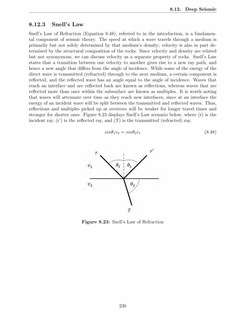
8.12. Deep Seismic
8.12.3 Snell’s Law
Snell’s Law of Refraction (Equation 8.48), referred to in the introduction, is a fundamen-tal component of seismic theory. The speed at which a wave travels through a medium isprimarily but not solely determined by that medium’s density; velocity is also in part de-termined by the structural composition of the rocks. Since velocity and density are relatedbut not synonymous, we can discuss velocity as a separate property of rocks. Snell’s Lawstates that a transition between one velocity to another gives rise to a new ray path, andhence a new angle that differs from the angle of incidence. While some of the energy of thedirect wave is transmitted (refracted) through to the next medium, a certain component isreflected, and the reflected wave has an angle equal to the angle of incidence. Waves thatreach an interface and are reflected back are known as reflections, whereas waves that arereflected more than once within the subsurface are known as multiples. It is worth notingthat waves will attenuate over time as they reach new interfaces, since at an interface theenergy of an incident wave will be split between the transmitted and reflected waves. Thus,reflections and multiples picked up at receivers will be weaker for longer travel times andstronger for shorter ones. Figure 8.23 displays Snell’s Law scenario below, where (r) is theincident ray, (r’) is the reflected ray, and (T) is the transmitted (refracted) ray.
sinθ1v2 = sinθ2v1 (8.48)
Figure 8.23: Snell’s Law of Refraction
230

8.12. Deep Seismic
8.12.4 Fermat’s and Huygen’s Principles
Fermat’s principle states that the path taken between two points by a ray is the path thatis traversed in the shortest amount of time. Fermat’s principle is helpful in describing theproperties of rays that are reflected off of rock boundaries or rays that are refracted throughboundaries.
Huygen’s principle states that every point on a wave front may be considered a sourceof secondary spherical wavelets which spread out in the forward direction.
8.12.5 Velocity As a Physical Property of Rock
The velocity at which seismic waves propogate through rock tend to increase with depth dueto the increase in pressure and subsequent compaction of the rock [12]. Shales are a softrock and especially susceptible to the compaction at greater depths, therefore the velocityinherent in shales is widely variant [12]. We would generally expect to see reflections fromshale/sandstone boundaries, but if they have the same velocities due to compaction at cer-tain depths, there is no impedance contrast and no reflection. Granitic rocks on the otherhand, tend to form at greater depths and because of a high density crystalline composition,naturally have a considerably higher velocity than sedimentary rocks [23]. Therefore, we al-most always expect to see a strong reflection from crystalline basement rock and sedimentaryrock boundaries.
8.12.6 Geophones
Geophones, as seen in Figure 8.24 are small instruments that work via the principles ofinduction, which can be described mathematically by Faraday’s law. Within the geophone,a small magnet within a coil remains relatively stationary as the coil, accelerated by seismicenergy or surface waves, moves within the geophone enclosure, inducing a measurable current(see Figure 8.25). The magnitude of this current tells us something about the relative energyof the seismic event.
Figure 8.24: Standard Geophones that are used in receiving a seismic signal
231

8.12. Deep Seismic
Figure 8.25: A simple schematic showing the inside of a geophone and how it works
8.12.7 CMP Gatherers
To explain CMPs, we are forced to make several restrictive assumptions: First, that theboundary between two layers of varying velocities is perfectly horizontal, along with thesurface. Second, that the velocity of these layers is homogeneous; that is, the velocity doesnot vary within the layer. Third, that these layers are isotropic, meaning that the propertiesfor the medium are uniform in all directions.
This implies that a wave traveling through a medium in one direction would behave thesame as if that wave were to travel through the medium in a different direction. Addition-ally, it is important to emphasize that these gathers also have the same depth, or commondepth point (CDP).
In seismic, the usage of the terms CMP and CDP are virtually interchangeable; however,CMP emphasizes the common alignment of points along the vertical axis whereas CDP em-phasizes the alignment of points along the horizontal axis.
In a CMP gather, the travel time increases hyperbolically as offset increases, in accordancewith equation 8.49. Here, Tx is the two-way travel time, T0 is the travel time at zero offset,xis the offset, and vs is a parameter called the stacking velocity.
232

Figure 8.26: CMP Gather
Sorting data into CMP gathers allows us to increase the signal-to-noise SNR ratio. Ifwe define n to be a single trace in a gather, then the SNR increases by a factor of
√n as the
number of traces increases. Furthermore, here we can define a quantity called ”fold”, whichis simply a word for the number of traces that highlight a particular point in the subsurface.For instance, if there are five shots in a CMP gather, then the fold here is five.
T 2x = T 2
0 + (x/vs)2 (8.49)
8.12.8 Fold
Fold, as referred to in seismic aquisition, relates to how many times a common midpoint issurveyed. A common midpoint is used in multichannel seismic acquisition, where a pointhalfway between the source and the receiver is shared by numerous source-receiver pairs.The redundancy of imaging the midpoint muliple times allows for a better signal to noiseratio. This will allow for true reflection to be represented numerous times by signal, whichwill make it appear better in the shot data, where as noise is often times random and willbe cancelled out. The higher the fold is, the better the shot records and images will be.Fold is increased by source points being closer together and by the number of sweeps beingincreased for each source point.
233

BIBLIOGRAPHY
[1] Colorado oil and gas conservation comission. Online Database.
[2] Digital-multimeter. Image.
[3] Electrodes. Image.
[4] Flux diagram. Image.
[5] Self-potential set-up. Image.
[6] Wenner. Image.
[7] Althos. Global positioning system - gps, 2009.
[8] Amazon. Garmin etrex 30 worldwide handheld gps navigator, 2014.
[9] Mark N Berdichevsky and Vladimir I Dmitriev. Models and methods ofmagnetotellurics. Springer, 2008.
[10] Chris Braning. Braning land surveying, February 2009.
[11] Gerry Clarkson and Marshall Reiter. The thermal regime of the san juan basin sincelate cretaceous times and its relationship to san juan mountains thermal sources.Journal of volcanology and geothermal research, 31(3):217–237, 1987.
[12] J.A. Coffeen. Seismic Exploration Fundamentals, Second Edition. PennWell PublishingCompany, 1421 South Sheridan Road/P.O. Box 1260, Tulsa, Oklahoma 74101, 1986.
[13] Curtis D Conley. Geology of the Chromo Anticline Archuleta County, Colorado andRio Arriba County, New Mexico. PhD thesis, Colorado School of Mines, 1958.
[14] T. Dahlin and B. Zhou. A numerical comparison of 2d resistivity imaging with 10electrode arrays. Geophysical Prospecting, 52:379–398, 2004.
[15] Michael J Galloway. Hydrogeologic and geothermal investigation of pagosa springs,colorado. Technical report, Colorado Geological Survey, Denver (USA), 1980.
[16] Geonics.
234

[17] hydroGEOPHYSICS.
[18] Marvin Johnson. Personal Communication.
[19] F. Jones. Electrical resistivity of geologic materials, June 2007.
[20] F. Jones. Inversion theory: Practicalities: 2d resistivity as the example, 2007.
[21] Gareth Jones. Echolocation. Curren Biology, 15(13):R484–R–488, 2005.
[22] Vincent C Kelley. Pre-cambrian rocks of the san juan basin. 1950.
[23] Manoj Khandelwal. Correlating p-wave velocity with the physico-mechanicalproperties of different rocks. Pure and Applied Geophysics, 170(4), Apr2013.
[24] J Klein and JJ Lajoie. Practical geophysics for the exploration geologist, 1980.
[25] GC Kukal. Log evaluation of compacted shaly sands of the mesaverde group, uintabasin, utah. In Proc. Fourth Annual DOE Symposium (Aug., 1978) E, volume 2, 1976.
[26] Arun Kumar. Handheld gps surveying unit– fast and easy survey, May 2010.
[27] Rich Krahenbuhl. Yaoguo Li. Influence of Self-demagnetization Effect on DataInterpretation in Strongly Magnetic Environments(). 77th SSG, page All, 2007.
[28] Trimble Navigation Limited. How differential gps works, 2013.
[29] John C Lorenz and Scott P Cooper. Tectonic setting and characteristics of naturalfractures in mesaverde and dakota reservoirs of the san juan basin. New MexicoGeology, 25(1):2–14, 2003.
[30] Garmin Ltd. What is gps, 2014.
[31] John W Lund. Characteristics, development and utilization of geothermal resources.GHC Bulletin, 28(2):1–9, 2007.
[32] John Milsom. Field geophysics, volume 25. John Wiley and Sons, 2007.
[33] John Milsom and Asger Eriksen. The Geological Field Guide Series: Field Geophysics,Fourth Edition. John Wiley and Sons Ltd, Chichester, West Sussex, UK, 2011.
[34] E.A. Muiuane and L.B. Pedersen. Automatic 1d interpretation of dc resistivitysounding data. Journal of Applied Geophysics, 42:35–45, 1999.
[35] Department of Geophysics Field Camp. Geophysical investigation of the pagosasprings geothermal system. Technical report, Colorado School of Mines, 2013.
[36] Greg Pendleton. The fundamentals of gps, July 2002.
[37] Peter Reid. The earth’s magnetic field, 2011.
[38] A. Revil. Presentation revil.ppt, 2014.
235

8.12. Deep Seismic
[39] A. Revil, M. Karaoulis, T. Johnson, and A. Kemna. Review: Some low-frequencyelectrical methods for subsurface characterization and monitoring in hydrogeology.Hydrogeology Journal, 20:617–658, 2012.
[40] J.B. Rittgers and et. al. Karaoulis, M. Self-potential signals generated by the corrosionof buried metallic objects with application to contaminant plumes. Geophysics,78:EN65–EN82, 2013.
[41] Gerlinde Schaumann. Application of transient electromagnetics (tem) for theinvestigation of the electrical resistivity distribution in the subsurface at a potentialgeothermal site in tanzania-introduction of the protem57 instrument.
[42] S. Shearer. Three -dimensional Inversion of Magnetic Data in the Presence ofRemanent Magnetization(). Masters Thesis, Masters Thesis:All, 2005.
[43] Fiona Simpson and Karsten Bahr. Practical magnetotellurics. Cambridge UniversityPress, 2005.
[44] Kenneth Smith. Cesium Optically Pumped Magnetometers (). Geometrics, page 8,1997.
[45] Guochang Xu. GPS Theory, Algorithms and Applications. Springer, Heidelberg, NewYork, 2007.
[46] D.A. et al. Zimmerman. Al comparison of seven geostatistically based inverseapproaches to estimate transmissivities for modeling advective transport bygroundwater flow. Water Resources Research, 34:1373–1413, 1998.
236