GEOPHYSICS FOR MINERAL EXPLORATION

A Manual for Prospectors

Prepared for Matty Mitchell RoomNewfoundland and Labrador Department of Natural Resources

Prepared by

W.J. Scott, Ph.D., P.Eng., P.Geo.Consulting Geophysicistwilliamjscott@bell.net

February 2014

FOREWORD

This manual was generated as a result of persuasion by Norm Mercer, then MineralExploration Consultant with the Newfoundland Department of Natural Resources (NDNR),while the author was with GeoScott Exploration Consultants Inc. Both of these people are nowretired. The manual has benefitted greatly from contributions from Gerry Kilfoil and PhilSaunders, both of NDNR, and from Ron Verrall and Susan Scott, consultants.

Any errors that remain, however, are the responsibility of the author.

W.J. Scott Ph.D., P.Eng., P.Geo (NL)February 2014

Table of Contents

1.0 INTRODUCTION . . . . . . . . . . . . . . . . . . . . . . . . . . . . . . . . . . . . . . . . . . . . . . . . . . . . . . . . . . 1

2.0 MAGNETIC SURVEYS . . . . . . . . . . . . . . . . . . . . . . . . . . . . . . . . . . . . . . . . . . . . . . . . . . . . . 2

3.0 ELECTROMAGNETIC SURVEYS . . . . . . . . . . . . . . . . . . . . . . . . . . . . . . . . . . . . . . . . . . . . 43.1 VLF EM Surveys . . . . . . . . . . . . . . . . . . . . . . . . . . . . . . . . . . . . . . . . . . . . . . . . . . . . . 43.2 Horizontal Loop EM Surveys . . . . . . . . . . . . . . . . . . . . . . . . . . . . . . . . . . . . . . . . . . . 73.3 Time-domain EM Surveys (TEM, TDEM, Geonics EM37, Crone Pulse EM, UTEM,

etc) . . . . . . . . . . . . . . . . . . . . . . . . . . . . . . . . . . . . . . . . . . . . . . . . . . . . . . . . . . . . . 8

4.0 RADIOMETRIC SURVEYS. . . . . . . . . . . . . . . . . . . . . . . . . . . . . . . . . . . . . . . . . . . . . . . . . . 94.1 Introduction . . . . . . . . . . . . . . . . . . . . . . . . . . . . . . . . . . . . . . . . . . . . . . . . . . . . . . . . . 94.2 Radioactive Decay . . . . . . . . . . . . . . . . . . . . . . . . . . . . . . . . . . . . . . . . . . . . . . . . . . . . 94.3 Instruments for detecting radioactivity . . . . . . . . . . . . . . . . . . . . . . . . . . . . . . . . . . . . 9

5.0 INDUCED POLARISATION SURVEYS . . . . . . . . . . . . . . . . . . . . . . . . . . . . . . . . . . . . . . . 125.1 Introduction . . . . . . . . . . . . . . . . . . . . . . . . . . . . . . . . . . . . . . . . . . . . . . . . . . . . . . . . 125.2 IP measurements: Electrode arrays . . . . . . . . . . . . . . . . . . . . . . . . . . . . . . . . . . . . . . 125.3 Multi-dipole Surveys . . . . . . . . . . . . . . . . . . . . . . . . . . . . . . . . . . . . . . . . . . . . . . . . . 155.4 Gradient Surveys . . . . . . . . . . . . . . . . . . . . . . . . . . . . . . . . . . . . . . . . . . . . . . . . . . . . 16

6.0 GRAVITY SURVEYS . . . . . . . . . . . . . . . . . . . . . . . . . . . . . . . . . . . . . . . . . . . . . . . . . . . . . 186.1 Introduction . . . . . . . . . . . . . . . . . . . . . . . . . . . . . . . . . . . . . . . . . . . . . . . . . . . . . . . . 186.2 Corrections needed in gravity surveys. . . . . . . . . . . . . . . . . . . . . . . . . . . . . . . . . . . . 186.3 Interpreting gravity survey data. . . . . . . . . . . . . . . . . . . . . . . . . . . . . . . . . . . . . . . . . 19

7.0 SEISMIC SURVEYS . . . . . . . . . . . . . . . . . . . . . . . . . . . . . . . . . . . . . . . . . . . . . . . . . . . . . . . 22

8.0 MULTIPLE METHODS AND SURVEY DESIGN . . . . . . . . . . . . . . . . . . . . . . . . . . . . . . 23

9.0 REFERENCES . . . . . . . . . . . . . . . . . . . . . . . . . . . . . . . . . . . . . . . . . . . . . . . . . . . . . . . . . . . 25

Appendix A: Interpretation of MaxMin Horizontal Loop EM Data

Appendix B: Induced Polarisation: Basis and Measurement Modes

Appendix C: List of Acronyms, Symbols and Terms

List of Figures

Figure 1: Total magnetic field map, central Newfoundland. . . . . . . . . . . . . . . . . . . . . . . . . . . . . . 2

Figure 2: Model VLF EM dip angle profiles. . . . . . . . . . . . . . . . . . . . . . . . . . . . . . . . . . . . . . . . . 5

Figure 3: VLF EM surveys over an area near Chalk River, Ontario. . . . . . . . . . . . . . . . . . . . . . . . 6

Figure 4: Typical MaxMin horizontal loop profile. . . . . . . . . . . . . . . . . . . . . . . . . . . . . . . . . . . . . 8

Figure 5: Typical ( ray spectra. . . . . . . . . . . . . . . . . . . . . . . . . . . . . . . . . . . . . . . . . . . . . . . . . . . 10

Figure 6: Electrode arrays used for IP surveys. . . . . . . . . . . . . . . . . . . . . . . . . . . . . . . . . . . . . . . 13

Figure 7: Method of plotting pseudosection of IP data. . . . . . . . . . . . . . . . . . . . . . . . . . . . . . . . . 14

Figure 8: Typical pseudosection, time-domain IP survey. . . . . . . . . . . . . . . . . . . . . . . . . . . . . . . 14

Figure 9: Results of inversion of part of pseudosection in Figure 8 . . . . . . . . . . . . . . . . . . . . . . 15

Figure 10: Gradient IP and resistivity survey near Baie Verte. . . . . . . . . . . . . . . . . . . . . . . . . . . 17

Figure 11a: Gravity map showing data with latitude, free air and Bouguer corrections. . . . . . . . 20

Figure 11b: Gravity data of Figure 11a, with linear regional trend removed from data. . . . . . . . 21

Appendix AFigure A1: Horizontal loop EM curves for two crossing angles and three dips . . . . . . . . . . . . A2

Figure A2: Characteristic curves for horizontal-loop system over a dipping sheet. . . . . . . . . . A3

Appendix BFigure B1: Membrane and electrode polarisation effects. . . . . . . . . . . . . . . . . . . . . . . . . . . . . . B1

GEOPHYSICS FOR MINERAL EXPLORATION

1.0 INTRODUCTION

The purpose of carrying out geophysical surveys is to find out something about the rocksin the survey area. Geophysical methods all depend on measuring a physical property of rocks. There are only a few such properties, shown in Table 1:

Table 1: Geophysical properties useful for surveys, roughly in order of increasing survey cost.

Property Typicalrocks/minerals

GeophysicalMethods

Notes

Magneticsusceptibility

Magnetite, ultra-mafics, iron-richrocks

Magnetic Mainly used for geologicmapping, sometimes foridentifying magnetitebodies or kimberlites.

ElectricalConductivity sigma (F) orResistivity rho (D)

F = 1/ D

Metallic sulphides,serpentinite, graphite,water-filled shears,salt water

Electromagnetic(EM)

VLF EMFrequency-domain(MaxMin), Time-domain(TEM or TDEM, PulseEM) finds conductiveminerals, but not sphalerite

Radioactivity Potassium(feldspars), Uranium,Thorium

Radiometric,gamma-rayspectrometry

Surveys generally respondonly to sources at or verynear the surface.

ElectricalPolarisability

Metallic sulphides,graphite, serpentinite,magnetite

InducedPolarisation (IP)

Time-domain, frequencydomain or phase angle. Finds massive ordisseminated metallic sulphides, but notsphalerite.

Density Sulphides includingsphalerite, barite

Gravity Can find sphalerite andother sulphides, useful forgeologic mapping.

Seismic velocity Massive sulphideshave higher velocitiesthan barren rocks.

Seismicreflection orrefraction

Generally used to mapstructure in 3D, sometimesto identify massive sulphidebodies. Can lookkilometres deep. Is veryexpensive.

2

Geophysical surveys generally look for concentrations of anomalously high values of theproperty being measured. The results of the survey are used to identify a target of interest, or tocorrelate the spatial variation of values of the property with variations in the geology. Thus theprimary reasons to do geophysics are to get information on geology, and possibly to find targetsof economic interest.

2.0 MAGNETIC SURVEYSThe earth has a magnetic field which behaves roughly like a bar magnet not quite lined up

with the earth’s north-south axis. In 2012, the north magnetic pole lay northwest of Resolute,and is drifting to the north and west. In 2015 it is predicted to be at 80.3N, 72.6W. In centralNewfoundland, a compass would point to magnetic north, about 20 degrees west of true north. In Newfoundland the magnetic field of the earth is inclined downwards at about 68 degrees to thehorizontal. The field interacts with the rocks through which it passes. If the rocks are magnetic(have high susceptibility) they become magnetised, and their field adds to that of the earth. Thusthe total magnetic field is stronger over magnetic rocks. Magnetic fields are measured innanoteslas (nT), which used to be called gammas (().

Magnetic surveys are carried out with magnetometers, which measure the total magneticfield with high precision. Because the earth’s magnetic field varies slightly from day to night,and with solar activity, it is important to use a base station magnetometer to record the daily ordiurnal changes in the magnetic field at a fixed point. The base station should be established inan area with low spatial magnetic variation. The base-station values can be used to correct thereadings taken with a roving magnetometer. Typically, magnetic readings are taken at fixedintervals (12.5 m or even 5 m) on grid lines. Some magnetometers are coupled to GPS receivers. They can be operated in ‘walking’ mode, with readings taken either at fixed time intervals or at

Figure 1: Total field magnetic map, central Newfoundland. The dashed lines are axes of weakHLEM conductors, generally parallel to the structure indicated by the magnetic contours. (NDNR Geofile 012A_1312)

3

fixed distances taken from the GPS positions. Reconnaissance surveys with a walkingmagnetometer and GPS do not require a cut grid. Magnetometer operators should ensure thatthey do not carry any strongly magnetic items such as an axe or geological hammer, which mightinfluence readings.

Magnetic maps are interpreted in terms of geology. Low-susceptibility rocks such aslimestones show as areas of low and relatively uniform magnetic fields, while mafic andultramafic rocks show as areas of higher and more variable magnetic fields. Comparison ofmagnetic readings in areas of known geology allows extrapolation of the geology into areaswhere the rocks are covered. Less frequently, magnetic surveys are used to outline areas withhigh concentrations of magnetite, potentially as sources for iron ore. To help visualise thedistribution of values, colour is employed. In geophysical displays, deep blues denote the lowestvalues, while reds and purples identify the highest readings. A scale bar is usually included toshow the range of values.

Figure 1 shows a total field magnetic map from an area in central Newfoundland (NDNRGeofile 012A_1312). The magnetic survey outlined three distinct zones where the magnetic fieldranges from a low of 150 nT (blue areas) to a high of 500 nT (red areas). Note that this is arelatively low range of magnetic field values. Although there are three distinct zones, none of theunderlying rocks is strongly magnetic. Also shown on this map are axes of weak electromagneticcouductors (see discussion in Part 3.2 below), generally aligned with the edges of the magnetically indicated rocks.

The central part of the grid (blue area) has the lowest magnetic expression, whereas theareas to the grid north and grid south (yellows through reds) are more magnetic. Because of thelack of outcrop information in the area it is difficult definitively to correlate these zones withbedrock geology. An outcrop of visibly altered felsic volcanics appears to be located between thenorthwest magnetic high and the central low. It is possible that the grid north high is correlativewith a plagioclase and blue quartz porphyritic felsic tuff unit, even though it was not noted to bemagnetic. On the same basis, the grid south high may be correlated with a unit of maficvolcanics which was noted to be weakly magnetic at one sample location. Without the magneticmap, it would be difficult to make any deductions about the geology.

4

3.0 ELECTROMAGNETIC SURVEYS

Electromagnetic (EM) surveys use a transmitter to generate a time-varyingelectromagnetic field in the earth, known as the primary field. This field gives rise to small time-varying voltages in the earth. Where the earth is conductive, the voltages drive small time-varying flows of current, which give rise to electromagnetic fields of their own called secondaryfields. The primary and secondary fields add together.

EM surveys measure the earth’s willingness to conduct electricity, or conductivity (F insiemens/m). The higher the conductivity, the more current will flow in the earth for a givenelectrical field strength. If the earth is not conductive, the unwillingness of the earth to conductelectricity is expressed in resistivity (D in ohm-metres). The higher the resistivity, the lesscurrent will flow for a given electrical field strength. At low frequencies, conductivity andresistivity are inversely related: F = 1/D.

3.1 VLF EM SurveysThe simplest EM technique is VLF EM. For VLF (very low frequency)EM, the

transmitters are operated for communication purposes by the United States and other countriesfor communication with their submarines. The frequencies are typically at around 20 kilohertz(KHz). In terms of radio transmission, this is a very low frequency. VLF EM surveys can becarried out either with a Geonics EM16 or with a Crone Radem. In addition, mostmagnetometers offer the option of including VLF measurements at the same time. Survey linesare usually laid out to be roughly at right angles to the direction to the transmitter station.

Figure 2 shows model VLF EM profiles over a vertical conductive dyke at depths from10 to 200 metres, calculated after the method of Fraser (1969). The surface projection of theconductor is at the crossover point. If the two halves of the profile are symmetrical, as in Figure2, then the conductor is vertical. If the profile is not symmetrical, then the larger peak lies overthe down-dip side of the conductor. As depth increases, the separation between positive andnegative peaks increases, but there is no simple theoretical relationship. The signal from aVLF transmitter generates an alternating sheet of current in the earth, with the flow directioneverywhere oriented towards the transmitter. If the resistivity of the rocks is everywhereuniform, then the current sheet is uniform as well. However, if, for example, an appropriately-oriented long shear zone of 1 000 ohm-metres (S-m) lies in a host of 10 000 S-m, then thecurrent sheet will be deformed and ten times as much current will flow in the shear zoneas in the host rocks. The shear zone will give rise to a strong VLF anomaly, even though it doesnot have a very low resistivity. As a result of this phenomenon, known as current channeling,many VLF anomalies are generated by geological features which do not necessarily carrysulphides. Thus a VLF survey is an aid in mapping geological structure, rather than just a meansof finding conductors which could be hosts to economic mineralisation. Current channeling enhances the response of features with significant strike length, generating in them strongeranomalies than in short conductors with the same resistivity contrast.

Consequently, for a conductor to have a VLF anomaly, it must strike generally towardsthe VLF transmitter. Thus, not all conductors will be detected in a VLF EM survey with a single

5

transmitter azimuth. In Newfoundland the useable transmitters are in Cutler (Maine), Seattle(Washington), and possibly Rugby (England). The great-circle bearings (determined by laying astring on a globe to connect the transmitter and the field area) of all these transmitters lie within 15 degrees of each other, at about 105 degrees. Thus a long conductor striking generally south-westerly will give rise to a significant anomaly, while the same conductor striking northwesterlywill produce a much weaker VLF anomaly.

For example, Figure 3 shows the impact of local transmitter bearing on conductordetectability. The survey is from an area near Chalk River in Ontario, where fortuitously theazimuths of Cutler and Annapolis (then still in operation) differed by 87 degrees. Figure 3ashows the results of a survey using Cutler as the transmitter, and Figure 3b the results of a surveyusing Annapolis as the transmitter. Obviously neither survey alone could have identified all theVLF conductors in the area. To be detected in a survey using one transmitter, conductors mustbe well-coupled to that transmitter, by striking generally towards that transmitter. Conductorsstriking at right angles to the transmitter direction are poorly coupled to it, and will not bedetected in a survey using that transmitter.

One recent problem in performing VLF EM surveys is that the stations do not necessarilytransmit at the times desired. Until lately it has been possible to obtain transmitting schedulesfrom the US Naval Observatory in Washington, but this information is no longer available.

Figure 2: Model VLF EM dip angle profiles for a conductive vertical dyke, calculated by themethod of Fraser (1969) for depths from 10 to 200 metres.

6

Three websites recommended by Geonics that often have information about past and presentVLF transmitter activities are:

http://moondog.astro.louisville.edu http://www.sidstation.loudet.org (SID Monitoring Station A118 Home Page) http://www.radiotelescopebuilder.com

There is a solution to the twin problems of poorly-coupled conductors and unpredictabletransmission times. It is possible to use a local transmitter, the TX27, which is available fromGeonics in Toronto. With a TX27 one can use a long wire grounded at the ends, laid a kilometeraway from the survey area, at right angles to the desired conductor orientation. This arrangementwill generate a reasonably uniform VLF field over an area of several square kilometres.

Figure 3: VLF EM surveys over an area near Chalk River, Ontario. (a) Survey using NAACutler, Maine, due east of site, on survey lines from south to north. (b) Survey using NSSAnapolis, Maryland, due south of site, on survey lines from east to west. (After Dence andScott, 1979).

7

3.2 Horizontal Loop EM SurveysThe most common horizontal loop EM (HLEM) system is the Apex MaxMin. In an

HLEM survey, there are two coils or loops. One of these loops is the transmitter, whichgenerates an alternating EM field (the primary field) in the ground beneath. If there is a conductor in the ground, then small circulating currents will flow in the conductor, and give riseto their own EM field (the secondary field) at the surface.

The other loop is a receiver. In the MaxMin the receiver loop is wound around twomagnetic cores, which form the ‘horns’ on the receiver. Normally the primary field is muchstronger than the secondary field. In order to detect the secondary field, a small part of theprimary field is sent from the transmitter via cable to the receiver, and is used to cancel theprimary field at the receiver, leaving only the secondary field to be detected.

The receiver measures two quantities, the in-phase component and the quadraturecomponent of the secondary field, expressed as a percentage of the primary field at the receiver. There is a phase shift or time delay in generating the secondary field of the conductor. The partof the secondary field that is not delayed is the in-phase component, and the part that is delayed isthe quadrature component. Anomalies from good conductors have large in-phase and smallquadrature components, while weaker conductors have low in-phase and high quadraturecomponents.

The MaxMin offers a range of frequencies which depends on the model. Typicalfrequencies increase from 110 hertz (Hz) by factrs of two to 3550 Hz or even higher. In amineral exploration survey, both lowest and highest frequencies are read, but not all intermediatefrequencies are necessarily used.

Interpretation of HLEM data depends on the assumption that the transmitter and receivercoils are coplanar (that is, in the same plane) at a constant separation. In areas of topography,maintaining this assumption is not trivial. The MaxMin system allows the operator to measurethe slope to the next station before leaving the current one. If this measurement is done at eachstation, the computer in the MaxMin receiver will integrate the slope readings to determine theelevation difference between the Tx and Rx coils. It will then display the tilt required for coilcoplanarity, and also the amount of extra separation to be used to account for the cable drapingover topography.

Figure 4 shows a typical HLEM profile over a conductor. Note that the anomalyamplitude increases with the frequency. In this example, in-phase and quadrature componentsare roughly equal, implying an intermediate conductor strength. For a discussion ofinterpretation procedures for HLEM data, see Appendix A.

The separation between the transmitter and receiver coils controls the depth at whichconductors can be found. With the MaxMin, spacing between transmitter and receiver can be25 m, 50 m, 100 m, 200 m or more, depending on the power of the transmitter. A rule of thumbis that good conductors will be found if they are shallower than half the coil separation.

8

3.3 Time-domain EM Surveys (TEM, TDEM, Geonics EM37, Crone Pulse EM, UTEM, etc)Transmitters for time-domain EM systems usually use large rectangular loops laid on the

ground, typically with sides hundreds of metres long. The waveform of the transmitted signal isdesigned to produce repeated bursts of energy. Typical waveforms are half-sine (Crone Pulse EM), triangle waveform (UTEM), turn-off ramp function (Protem) and other repetitive signals. Each impulse of energy travels down into the earth, generating time-decaying currents in anyconductor within range. By monitoring the signal in the off time after the transmitted pulse, it ispossible to detect the fields of these decaying currents.

From the character of the decay fields it is possible to determine depth, shape andapproximate conductance of the anomalous bodies. Discussion of interpretation techniques fortime domain EM is beyond the scope of this manual. However, an extensive discussion ispresented in Chapter 7 of Telford et al. (1990).

In the use of TDEM for exploration for nickel, it has been found that the conductivity ofmassive nickel sulphide bodies is very high. As a result, some of the energy in the transmittedpulse is absorbed immediately by the sulphides, and the resulting transient is thus reduced. Inorder to detect such massive nickel sulphides, it is necessary to measure the transmitted pulse,and determine its deformation. At Voisey’s Bay, for example, normal off-time transientsgenerated stronger anomalies outside the massively-conductive Ovoid than in it. In order to mapthe anomaly generated by the Ovoid, it was necessary to measure the field during the on-time andcompare the predicted and measured waveforms. UTEM, however, already measures during thetransmission time and is not subject to the same limitation.

Figure 4: Typical MaxMin profile, 100 m coil separation, 25 m station interval, with threefrequencies: 220Hz, 880Hz and 3555Hz. (Unpublished data).

9

4.0 RADIOMETRIC SURVEYS.

4.1 IntroductionThe discussion in this section is based on Telford et al., (1990). Although there are at

least 20 known naturally-occurring radioactive elements, the only ones of significance ingeophysical prospecting are uranium (U), thorium (Th) and an isotope of potassium ( K). One40

other, rubidium, is useful in determining the age of rocks, but the rest are either so weak, so rare,or both, as to be of no significance in applied geophysics. The two elements uranium andthorium are important as sources of fuel for the generation of heat and power in nuclear reactors. Large parts of the world have been surveyed on the ground and particularly from the air, in thesearch for uranium.

4.2 Radioactive DecayThe radiation from naturally-occurring radioactive elements consists of three distinct

types: alpha ("), beta ($) and gamma (() radiation. All three types of rays can producescintillations or phosphorescence in certain minerals and chemical compounds. In addition theyionize gas, making it electrically conducting, and they affect photographic emulsions in much thesame way as light or X-rays.

The three rays have very different penetrating powers. Thus, " rays are easily stopped bya piece of paper, and $ rays are easily stopped by a few millimetres of aluminum. Theattenuation of ( rays requires several centimetres of lead. The range of " and $ rays inoverburden or rock is virtually zero, while ( radiation can pass through from 50 to 75 mm ofrock.

4.3 Instruments for detecting radioactivityThere are two principal instruments, the Geiger counter, and the scintillometer. The (-

ray spectrometer is an extension of the scintillometer.

The Geiger-Müller counter is a simple device that responds primarily to $ radiation. Thedetector is a thin-walled cylindrical tube with a very thin mica window in the end to permit theentry of the $ radiation. The tube consists of an axial anode wire and a coaxial cathode cylinderpolarised by several hundred volts, and is filled with an inert gas such as argon at low pressure. Radiation entering the tube ionizes gas molecules, and the positive ions and electrons areaccelerated to the cathode and anode respectively. These charges also ionize other gas atoms enroute, so that the original entering ray produces an avalanche of charged ions that cause asubstantial discharge pulse across the anode resistor. This pulse is amplified to produce a clickin a speaker or headphones. Additionally, successive pulses charge a capacitor and the chargeleaks off through a microammeter, which registers a current proportional to the strength of thecharge entering the condenser.

The prospecting Geiger counter is simple and cheap. However it has little else torecommend it. It must be held close to the outcrop to detect the $ rays, and is thus a tool oflimited application, seldom used in modern prospecting.

10

The scintillometer works by counting scintillations produced in a detector by ( radiation. The most efficient detector is made by growing natural crystals of sodium iodide (NaI), treatedwith thallium (Tl). The NaI is transparent to its own fluorescent emission, and all faces but one

are coated with light-reflectingmaterial. If the crystal is largeenough, then the conversionefficiency for natural ( radiationis close to 100%.

Light generated in theNaI crystal by ( radiation isamplified through aphotomultiplier tube; the outputcurrent is applied across aresistor to produce a voltagepulse which is amplified and integrated as in the Geigercounter. The great advantage ofthis instrument is in theefficiency of ( radiationdetection, but it will also detect$ radiation. The instrument issomewhat larger and heavierthan the Geiger counter, andalso more expensive.

A logical extension ofthe scintillometer is aspectrometer that distinguishescharacteristic ( rays from K, U40

and Th. Such instruments arewidely used in airborne surveysand some portable units are alsoavailable. The intensity of thelight pulse, and thus the

amplitude of the output voltage pulse, are proportional to the initial ( ray energy. ( radiationfrom different sources has different energy levels. The output spectrum of the spectrometer iscomplex, and has peaks which are associated with the energy of radiation from different sources. Figure 5 shows typical pulse-height spectra for different geological sources. To obtain aspectrum, the relative count rate of incoming ( radiation, is plotted against the energy measuredin millions of electron volts (MeV). In a field situation, some ( rays lose energy by scattering inescaping from the source, and also during passage through the air to the crystal. In addition,some of the ( rays lose only part of their energy within the NaI crystal. This, coupled with thefact that the U and Th series emit numerous ( rays over a wide energy range, results in a complexpulse-height spectrum, as shown in Figure 5.

Figure 5: Typical ( ray spectra for Th, U, a granite gneiss andK, after Telford et al, 1990, p624.40

11

All four curves in Figure 5 have characteristic peaks. The pure potassium sampleproduces a relatively simple curve having only the K peak at 1.46 MeV. Thorium is40

characterised by the strong 2.62 MeV peak of Tl (thallium), a constituent of the Th decay208

series. The uranium spectrum is most complex, although the peak at 1.76 MeV (million electronvolts) is reasonably distinctive. Potassium and thorium are clearly evident in the spectrum forthe granite gneiss. A small fraction of uranium is also indicated.

A prospecting spectrometer should be able to isolate the K, U and Th peaks at 1.46, 1.76and 2.62 MeV. It should use at least three separate channels, each sensitive to one of the energypeaks. Generally the channel centres and widths are adjustable.

Normally ground radiometric surveys are used as followup after airborne surveys. Airborne spectrometers can use much larger crystals, measure more channels and correct both fordrift and background radiation. Ground surveys can then help to isolate the sources of theairborne anomalies. The interpretation of ground survey results are mainly qualitative. This ispartly due to the extremely small depth of penetration possible with the method. It is also theresult of the inherent complexity of the ( ray spectra.

For many years, radiometric surveys, both airborne and ground, have been primary toolsin the exploration for uranium. In addition, thorium often is associated with Rare Earth Element(REE) minerals, Thus, airborne gamma-ray spectrometric surveys are a key tool in theexploration for REEs. Similarly, K response can be used to identify zones of potassic alteration,and thus contribute to geological mapping based on geophysical survey results.

12

5.0 INDUCED POLARISATION SURVEYS

5.1 IntroductionElectric current in rocks is usually carried by the movement of charged ions in the water

which fills the pores. If a pore is blocked by a metallic substance such as a metallic sulphide,then the current flow must transfer to the sulphide, where it is carried by the movement ofelectrons. As a result there is a small delay at the interface while the charged ion loses its chargeeither by taking on an electron from the metal or by releasing one into the metal. Because of thisdelay, a concentration of ions, waiting to lose or gain an electron, develops at the interface duringthe flow of current. When the current is interrupted, the ion concentration disperses away fromthe interface, and this drift is seen as a transient voltage along the pore. Thus inducedpolarisation (IP) arises at the interfaces between pores and metallic sulphides. The strength of anIP response is governed not by the volume of sulphides in the rock, but by the amount ofsulphide surface exposed to the pore water. A certain volume of fine-grained sulphide willgenerate a larger IP effect than the same volume of coarse-grained sulphide. Consequently thestrength of an IP anomaly is not necessarily an indication of the volume of metallic sulphidespresent. Because a rock showing IP effects can store electric energy, even though for short times,it is said to be chargeable, and the chargeability of a rock is a measure of the strength of its IPeffect. See Appendix B, Section B2, for a definition of chargeability.

A few other minerals can also generate IP effects. For instance, graphite carries currentby the drift of electrons, and thus gives rise to an IP effect. Similarly some magnetites, and evensome serpentinites have been known to generate IP responses. Note that non-metallic sulphidessuch as sphalerite do not give rise to an IP effect.

Appendix B amplifies the description of the development of IP effects. It also describesthe modes of measuring IP effects, and the units of the measurements.

5.2 IP measurements: Electrode arraysMaking IP measurements involves use of a transmitter to generate a current, and a

receiver to measure the resulting voltages. The transmitted current is injected through twotransmitter electrodes, and the received voltages are measured through two or more receiverelectrodes.

Transmitter electrodes are usually metal rods, although in some cases of high-resistivityareas, they may be metal screen or even aluminum foil buried in pits moistened with water. Receiver electrodes are often metal rods. For greater stability and lower noise levels, porouspots should be used. A porous pot is a small container with a porous bottom such as anunglazed ceramic disc, filled with a saturated solution of copper sulphate, with a copper electrodeinserted in the pot. Contact with the earth is through the fluid in the porous bottom of the pot,and the connection to the receiver is through the copper electrode. Porous pots give more stablemeasurements, particularly where the acidity of the ground varies along the measured profile(e.g. when the line varies from bog to dry earth).

13

Figure 6: Electrode arrays used for IP surveys. A and B are transmitter electrodes, M and N are

A A B B M Mreceiver electrodes. For the gradient array, co-ordinates are A(x , y ), B(x , y ), M(x , y ) and

N NN(x , y ), where the survey lines run parallel to AB. In multi-dipole and pole-dipole arrays, thedipoles are separated by distances which are multiples (n = 1, 2, 3, etc.) of the dipole size a..

14

IP measurement electrode arrays include multi-dipole, pole-dipole, pole-pole andSchlumberger and gradient. Figure 6 shows these arrays, and Section B.5 in Appendix B givesthe formulae for apparent resistivity for each of the arrays.

Figure 7:: Method of plotting to generate a pseudosection of IP or resistivity data.

Figure 8: Typical pseudosection, time-domain IP/resistivity, a = 25m, n = 1 to 6, apparentchargeability above, apparent resistivity below. Rectangle encloses data inverted for Fig. 9.

15

5.3 Multi-dipole Surveys

The most common arrays now are multi-dipole and pole-dipole. Data acquired by thesearrays are usually portrayed in pseudosections, which demonstrate the relative depth dependenceof the measurements in a schematic way. Figure 7 shows how a pseudosection is plotted frommulti-dipole data. For pole-dipole plots the diagonal for the transmitter is drawn from the onetransmitter electrode instead of from the centre of the dipole.

Figure 9: Results of inversion of central part of pseudosection data of Figure 8. .Chargeability values in millivolts per volt (mV/V), resistivity values in ohm-metres (S-m). White dots in models show centres of cells used for inversion. (Unpublished data)

16

However, it should be remembered that a pseudosection is not a geological section. Evensimple bodies such as dykes can generate complex anomaly patterns. If the pseudosection is fora multi-dipole array, then an anomaly over any body will be the same regardless of which sidethe transmitter dipole is of the receiver array. However, with the pole-dipole array, the shape ofthe anomaly depends on which side the transmitter electrode is of the receiver array.

Figure 8 shows a typical pseudosection of multi-dipole IP data, with chargeability datacontoured linearly at intervals of one mV/V, and resistivity data contoured logarithmically atintervals of 1, 3, 5, 10, 30 etc. It is increasingly frequent not just to present the pseudosections ofchargeability and resistivity, but also to invert the data and show the inverted sections as well. Figure 9 shows the inversion results for the area within the rectangle in the pseudosection ofFigure 8.

The inversion process predicts the field measurements for the model, and compares themto the observed field data. The error of the fit is calculated as the root of the average of thesquare of the difference between observed value and value predicted from the model. Anestimate of the reliability of the model can be made by looking at the fitting errors. In thisexample the resistivity fit is 2.61 percent. An error this small is quite acceptable. Similarly thechargeability fit is 0.70 per cent, which is remarkably good as well.

5.4 Gradient SurveysTo carry out a gradient survey, the two transmitter electrodes are established at points

outside the survey area, along the projection of the centre survey line. The transmitter separationcan be up to a few kilometres, provided enough current is transmitted to produce a large enoughsignal within the survey area. The receiver dipole can be whatever is appropriate for resolvingthe expected anomalies. Typical receiver dipole separations range from 25 to 100 metres.

The gradient array yields only one set of resistivity and IP measurements for each point. Consequently gradient data are usually portrayed as maps showing the spatial variation of thedata. A gradient survey is a useful tool for covering a large area in which the positions ofanomalies are not well known. Coverage with a gradient survey is much more rapid than with apole-dipole or multi-dipole array, because only the receiver electrodes must be moved. Figure 10shows the results of a gradient survey over an area 400 m east-west and 600 m north-south. Readings were taken with 25 metre dipoles, on lines 25 m apart. Layout of transmitter wire,survey of 6100 metres and pickup of transmitter wire required 14 survey hours.

Once a gradient survey has been carried out, and approximate anomaly positionsidentified, then suitable lines can be selected to carry out detailed surveys with multi-dipole orpole-dipole arrays. The detailed surveys then yield better definition of the anomalies.

17

Figure 10: Gradient IP and Resistivity survey near Baie Verte. Data from NDNR012H/16/1710.

18

6.0 GRAVITY SURVEYS

6.1 IntroductionThe earth exerts an attraction on any mass that is within its gravity field. The attraction

varies inversely with the square of the distance between the centre of the earth and the centre ofthe mass. We recognise this attraction as the “weight” of the mass. In a local situation, a givenmass will weigh more if the earth is more dense under it. This relationship is the basis of thegravity method. In gravity surveys the object is to locate, from irregularities in the earth’s gravityfield, small variations in density of rocks below the earth’s surface.

A gravimeter, used to measure the earth’s gravitational field, is a very sensitive weighscale. It has a small reference mass mounted on a hinged arm. The arm is held horizontally inplace by a spring which is adjustable. The spring is adjusted to move the mass to be in alignmentwith a reference mark. The adjustment to the spring is calibrated to read the local value of theearth’s gravity field. The gravimeter is a very delicate instrument which is sensitive to betterthan one part in ten million of the earth’s gravity field. Gravity measurements can outline localanomalies in the earth’s gravity field which are generated by local high-density bodies in theearth. The earth’s field is about 980 gals (the gal is named after Galileo, who first experimentedwith the earth’s gravity field), but significant gravity anomalies may be as small as 0.1 milligal,where one milligal (mgal) is about one millionth of the earth’s gravity, or one thousandth of agal.

6.2 Corrections needed in gravity surveys.Because the “weight” of a mass varies with the square of the distance to the centre of the

earth, small variations in elevation of the survey station can greatly affect the measured value ofgravity. As a result, it is necessary to correct for changes in location and elevation of the surveystations.

The first correction is known as the latitude correction. Because the earth rotates, itbulges at the equator, and flattens at the poles. Thus gravity is stronger at the poles than at theequator. In Newfoundland, the latitude correction is about 0.8066 mgal per north-southkilometre, and is subtracted as the survey station moves northward.

The second correction is the free-air correction. In Newfoundland, the earth’s field variesby about 0.197 mgal per vertical metre. If a station is above the reference datum, the correctionis added to the reading; if the station is below the reference datum, then the correction issubtracted from the reading. To calculate the latitude and free-air corrections to within 0.01mgal, the north-south location must be known within about 13 metres, and the elevation to about3 cm or better.

The third correction is known as the Bouguer correction. It accounts for the attraction ofmaterial lying between the station and the reference datum. The Bouguer correction is {0.04192 x (density of the intervening material)} per vertical metre. If the density of theintervening material is the average rock density of 2.67 grams per cubic centimetre (g/cc) then

19

the Bouguer correction is 0.112 mgal/metre. It is applied in the opposite sense to the free aircorrection, and is subtracted from the field reading when the station is above the referencedatum, and added when it is below.

The free-air and Bouguer corrections are often combined into the elevation correction. For a density of 2.67 g/cc, the combined correction is 0.19673 mgal/metre.

In areas of severe topography, a further correction, the terrain correction, is alsonecessary. When a mountain sits above a survey point, the upward attraction of the part of themountain above the station reduces the reading. Terrain corrections are complex, and, in pre-computer days, involved enormous amounts of hand calculation. Now, however, digitalprocessing uses digital terrain models to calculate terrain corrections. Surveys in areas of deeplakes must also allow for the reduction in the field readings because of the lower density ofwater. This correction is also performed digitally, provided care is taken to measure thedistribution of water depths.

Carrying out gravity surveys is not difficult, particularly because modern gravimeters areautomated in their measurement process. However, correcting raw gravity readings to producemeaningful values involves precise land survey. In open terrain, the usual approach to obtainingprecise corrections is to use a precise Global Positioning System (GPS) operated in a real-timekinetic mode (RTK). Note that a hand-held GPS does not offer adequate precision. The preciseGPS system uses a base station which tracks temporal changes in its position, and uses thechanges to determine positional corrections. In RTK mode, these corrections are broadcast inreal time. The survey station (the rover) is set at each survey point, and uses the broadcastcorrections to produce a precise position for the point. A GPS survey in RTK mode is capable ofhorizontal precision of less than a centimetre, with vertical precision about twice the horizontalprecision. However, if the sky is obscured by heavy vegetation, the GPS system may not seeenough satellites to be able to determine its position. In such areas, recourse must be had totraditional land survey techniques to fill in between GPS points.

In order to preserve the elevation precision needed for adequate corrections, when thegravimeter is set up at each station, the height of the instrument (HI) above the referenceelevation point is recorded. The value of HI is added to the ground elevation to obtain theelevation used in calculating corrections.

In performing gravity surveys, it is normal practice to establish a gravity base station,which is read at least at the beginning and end of the day, and sometimes more frequently. If asurvey is to be extended at a later date, using the same base station ensures that the two data setswill be seamless.

6.3 Interpreting gravity survey data.The final gravity data are usually plotted and contoured in the same manner as magnetic

data. Figure 11a shows a contour map of gravity data. The data set has had latitude, free air andBouguer corrections. Often gravity results such as these will show a gradual trend across the

20

area, which will distort local anomalies. The gradual trend in gravity values can arise fromdeep–seated geological variations, and can be removed from the data. The high gravity at thewest end and the low at the east end both disappear when a linear regional trend is removed(Figure 11b). Normally such trend removal is carried out by digital processing.

Gravity surveys are sometimes used as a follow-up to EM surveys, when there is apossibility that the conductor seen by the EM survey could be graphite. Sulphide bodies areusually more dense than the host rocks, and thus yield local high-gravity anomalies. Graphite, onthe other hand, is less dense than sulphides, and close in density to typical host rocks. Graphiteconductors do not usually give rise to local high-gravity anomalies. Gravity is also sensitive tothe presence of sphalerite, which is usually more dense than its host.

If the survey area is underlain by rocks of different densities, then gravity can be used tomap the distribution of each rock type.

Figure 11a: Gravity map showing contoured data with latitude, free air and Bouguer corrections. Contour interval 0.1 mgal (unpublished data).

21

Because the strength of a gravity anomaly falls off with the square of its depth, gravitysurveys cannot identify bodies buried deeper than a few hundred metres, no matter how high thedensity contrast.

Gravity has been very useful for identifying low-density accumulations of salt andpotash. Near Stephenville, there are large accumulations of salt and potash in the nearbyCarboniferous Bay St. George subbasin. The same rocks also host gypsum and anhydrite (higherdensity materials), which are often in close spatial association, which can make the interpretationof the data a bit tricky.

Figure 11b: Gravity data of Figure 11a, with linear regional trend removed from data. Contourinterval 0.1 mgal (unpublished data).

22

7.0 SEISMIC SURVEYS

Although seismic surveys are mainly employed for hydrocarbon exploration, there havebeen some recent applications to mineral exploration. Massive sulphide bodies have higherseismic velocities and densities than their host rocks. If the bodies are big enough, they can giverise to strong reflections. Surveys can be carried out in either two or three dimensions. Two-dimensional (2D) surveys yield single profiles, but are susceptible to errors generated byreflectors that are not directly under the survey line, but off to one side. Three-dimensional (3D)surveys involve observations on a full grid, with sources and receivers on various lines. 3Dsurveys are an order of magnitude more expensive than 2D ones. However, any major seismicsurvey is extremely expensive and extremely complex. Treatment of them is beyond the scopeof this manual.

Occasionally, shallow seismic refraction or reflection surveys are used to map thethickness of overburden, or to help in the exploration for and evaluation of granular mineraldeposits. For example, shallow seismic surveys were used to map the overburden thickness overthe Voisey’s Bay Ovoid deposit. The results provided input into the design of the open pit.

23

8.0 MULTIPLE METHODS AND SURVEY DESIGN

In many cases, more than one geophysical method can be used to help understand thegeological context of the geophysical survey results. For example, an electromagnetic surveymay have identified a conductor, but graphite is known to occur in the area. A small gravitysurvey can be carried out to see if the EM conductor is associated with higher density material. If there is no gravity anomaly then the conductor is not likely to arise from metallic sulphides.

The gravity method (including airborne gravity) is currently being used extensively in theLabrador Trough in the search for iron ore (Kilfoil, pers. comm.). It is not difficult to identifysurface outcrop of iron formations in this area with a magnetometer, However, these rocks are somagnetic (and variable) that much of the magnetic response (variability) is due to exposed orsubcropping ore, and this strong response masks any response of ore at depth. Thus there is nomagnetic way to determine how extensive the ore is. The rocks, at least in the southern Troughare also highly deformed and folded, so any realistic modelling of the magnetic data would benext to impossible. The gravity method is useful for distinguishing the wheat from the chaff; ithighlights the areas having significant subsurface accumulations. In the northern Trough, nearSchefferville, parts of these iron formations have been leached & high-graded to "direct shippingore", in which the magnetite has been completely replaced by hematite. The geophysicalsignature here is low magnetic readings associated with high gravity, lying along trend with verymagnetic, unaltered iron formations.

Within the limited size of this document, it has not been possible to include enoughexamples of field survey results. An excellent publication full of field examples is PracticalGeophysics III, recently published by the Northwest Mining Association.

When the use of geophysics is being considered, it is useful to go back to Table 1 (Page1) to help to define a geophysical approach. The first step is to identify the purpose of carryingout the survey. Is it to map geology, trace structure, and/or to search for concentrations ofparticular minerals? With the purpose identified, the next step is to ask what geophysicalproperties can be expected for the country rocks, the host rocks and the target body, and whatcontrasts in the properties will be needed to fulfill the purpose of the survey. At this point, itshould be evident which geophysical method or methods offer the best chance of meeting thepurpose of the survey.

If there is any doubt whether the best survey design has been achieved, it would be wiseto obtain qualified advice about the survey design, to be sure that the resulting survey generatesthe best possible outcome. An excellent source of qualified advice is the Matty Mitchell Roomin the Newfoundland Department of Natural Resources, whose staff can obtain advice frommany disinterested experts within the Department.

Before beginning a survey, it is important to ensure that the survey grid is laid out toenhance the response from the bodies of interest. Normally the grid is oriented so that the surveylines cross the strike of the expected target at right angles. If the results of an airbornegeophysical survey are available, then the grid can be oriented to cross interesting airborneanomalies at right angles.

24

Some targets, such as gold in quartz, may not have a geophysical property to help inexploration. However, it may be possible to find an indirect property, such as a property of thehost rocks, which will help in exploration. For example, the quartz rocks hosting gold may havevery high resistivity values. In this case a resistivity/IP survey may help in mapping thedistribution of high-resistivity quartz, which would help to concentrate exploration activity onsuitable host rocks.

As time passes, the fashion in mineral exploration can change, and targets which havebeen dismissed in the past may become attractive in the future. An example is graphite, whichfor many years has been considered a misleading pest in mineral exploration. Recent discoveryof high-grade graphite deposits has turned graphite from hateful villain to desirable target.

A valuable and largely under-used resource in mineral exploration with geophysics is theassessment files maintained by the Department of Natural Resources. Unless the area beingconsidered is truly unexplored, there will almost certainly be geophysical survey reports in theassessment files for the area under consideration. At the least, these reports can indicate whatsorts of results can be expected from specific geophysical techniques. At best, the reportedresults may contain anomalies associated with new or different targets, often neglected in theoriginal report. Before designing a survey on the basis of expected target responses, it veryuseful to see what results have been obtained in the past.

25

9.0 REFERENCES

Dence, M.R., and Scott, W.J., 1979. The Use of Geophysics in the Canadian radioactive wastedisposal program, with examples from the Chalk River Research Area: GeoscienceCanada, V6 no 4, 190-194.

Fraser, D.C., 1969. Contouring of VLF-EM data: Geophysics V34 no 6, December 1969,958-967.

Kilfoil, G., 2013, NDNR. Personal communication.

Northwest Mining Association. Practical Geophysics III for the Exploration Geologist, availableon CD-ROM from NWMA at (509) 624-1158 or e-mail at: www.nwma.org

Telford, W.M., Geldart, L.P., and Sheriff, R.E., 1990. Applied Geophysics, Second Edition:Cambridge University Press, 770 p.

Appendix A

Interpretation of MaxMin Horizontal Loop Data

Interpretation of MaxMin Horizontal Loop Profiles.

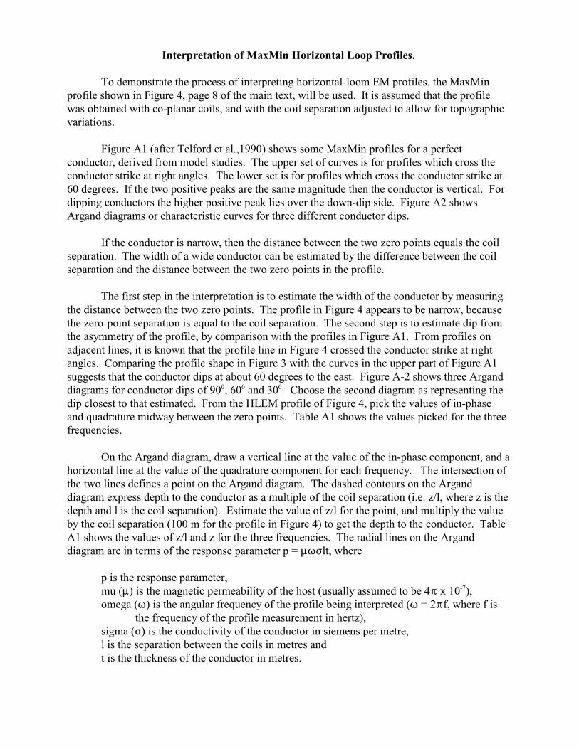
To demonstrate the process of interpreting horizontal-loom EM profiles, the MaxMinprofile shown in Figure 4, page 8 of the main text, will be used. It is assumed that the profilewas obtained with co-planar coils, and with the coil separation adjusted to allow for topographicvariations.

Figure A1 (after Telford et al.,1990) shows some MaxMin profiles for a perfectconductor, derived from model studies. The upper set of curves is for profiles which cross theconductor strike at right angles. The lower set is for profiles which cross the conductor strike at60 degrees. If the two positive peaks are the same magnitude then the conductor is vertical. Fordipping conductors the higher positive peak lies over the down-dip side. Figure A2 showsArgand diagrams or characteristic curves for three different conductor dips.

If the conductor is narrow, then the distance between the two zero points equals the coilseparation. The width of a wide conductor can be estimated by the difference between the coilseparation and the distance between the two zero points in the profile.

The first step in the interpretation is to estimate the width of the conductor by measuringthe distance between the two zero points. The profile in Figure 4 appears to be narrow, becausethe zero-point separation is equal to the coil separation. The second step is to estimate dip fromthe asymmetry of the profile, by comparison with the profiles in Figure A1. From profiles onadjacent lines, it is known that the profile line in Figure 4 crossed the conductor strike at rightangles. Comparing the profile shape in Figure 3 with the curves in the upper part of Figure A1suggests that the conductor dips at about 60 degrees to the east. Figure A-2 shows three Arganddiagrams for conductor dips of 90 , 60 and 30 . Choose the second diagram as representing the0 0 0

dip closest to that estimated. From the HLEM profile of Figure 4, pick the values of in-phaseand quadrature midway between the zero points. Table A1 shows the values picked for the threefrequencies.

On the Argand diagram, draw a vertical line at the value of the in-phase component, and ahorizontal line at the value of the quadrature component for each frequency. The intersection ofthe two lines defines a point on the Argand diagram. The dashed contours on the Arganddiagram express depth to the conductor as a multiple of the coil separation (i.e. z/l, where z is thedepth and l is the coil separation). Estimate the value of z/l for the point, and multiply the valueby the coil separation (100 m for the profile in Figure 4) to get the depth to the conductor. TableA1 shows the values of z/l and z for the three frequencies. The radial lines on the Arganddiagram are in terms of the response parameter p = :TFlt, where

p is the response parameter, mu (:) is the magnetic permeability of the host (usually assumed to be 4B x 10 ),-7

omega (T) is the angular frequency of the profile being interpreted (T = 2Bf, where f isthe frequency of the profile measurement in hertz),

sigma (F) is the conductivity of the conductor in siemens per metre,l is the separation between the coils in metres andt is the thickness of the conductor in metres.

A-2

For thin conductors the conductance, or strength of the conductor, is given by theconductivity-thickness product Ft, in units of siemens.

Table A1: Values for the profiles of Figure 3 for three frequencies.

Frequencyf (Hz)

T =2Bf

In-phase (%)

Quadrature (%)

Colour z/l Depth z(metres)

p Conductivity-thickness Ft(siemens)

222 1 395 -5 -7 Blue .25 25 3.7 21

888 5 580 -13 -15 Red .19 19 4.9 7

3555 22 337 -22 -20 Yellow .12 12 7.0 2.5

As the frequency increases, the profile amplitude of the anomaly also increases. Inaddition, the depth to the conductor appears to decrease, probably because the conductor is weaknear the surface, and improves in strength with depth. The values of Ft decrease with increasingfrequency, which is unusual. More often the value of Ft increases with increasing frequency.

Figure A1: Horizontal loop EM type curves for threedifferent dips and two different profile crossing angles,for a perfectly conducting half-plane (Ft approachinginfinity). After Telford et al. (1990).

A-3

Figure A2: Characteristic curves for horizontal-loop system over a dipping sheet, after Telford etal, 1990. Response parameter p = F:Ttl. See text for explanation. Coloured lines representvalues from the profile in Figure 4 on page 8.

Appendix B

Induced Polarisation: Basis and Measurement Modes

B.1 Basis of IP phenomena.All rocks contain at least very small amounts of water in their pores. Pure water is quite

resistive electrically. Water in rock pores, however, usually contains many dissolvedcompounds, which have dissociated into charged ions. For example, if salt (NaCl) is dissolvedin water, it dissociates into two types of ions: Na , with a positive charge, and Cl , with a+ -

negative charge. These ions are somewhat larger than the water molecules, and thus moveslowly through the water. If a battery were to be connected along the length of a pore with Na+

and Cl ions in the water, then the Na ions will drift towards the negative terminal of the battery,- +

and the Cl ions will drift towards the positive battery terminal. -

Most rock-forming minerals (quartz, feldspar, hornblende, etc.) are electrical insulators,and cannot carry any appreciable current. The exceptions are conductive minerals, such asmetallic sulphides (but not sphalerite) and graphite. In almost all rocks, therefore, electricalconduction is through the movement of charged ions in the water in the pores.

The generation of IPeffects can be due to eitherof two phenomena,membrane polarisation orelectrode polarisation. Figure B1 shows themechanisms involved. InFigure B1, pores in a rockare illustrated in a simplifiedmanner as layers ofelectrolyte between rockwalls. The upper pore inFigure B1(c) illustratesnormal conduction ofelectric current in a plainpore. If, however, there areclay particles exposed in thewalls of the pore, then thesituation is depicted inFigure B1(a). Because clayparticles have unsatisfiednegative charges on theirends, they attractconcentrations of loosely-bound positive ions. Whena voltage is imposed alongthe pore, as in Figure B1(b),the drift of charged ions isopposed by these boundconcentrations, particularlyif the pore is narrow. Theconcentrations of positiveions are deformed duringcurrent flow, and return to

Figure B1: Membrane and electrode polarisation effects (afterTelford et al. (1990).

B-2

their equilibrium positions when the voltage is removed. This return is seen as a small transientcurrent, which generates a small but measurable transient voltage which is measured as an IPeffect. This phenomenon is known as membrane polarisation. It occurs in almost all rocks, andgives rise to a small background IP effect.

Minerals that conduct electricity by the drift of electrons exhibit another form ofpolarisation known as electrode polarisation. Such minerals include the metallic sulphides, someoxides such as magnetite, ilmenite, pyrolusite and cassiterite, and, unfortunately for prospectinggeophysics, graphite. When a pore is blocked by a metallic sulphide particle, as in the lowerpore of Figure B1(c), the sulphide has a net surface charge on its faces as a result of the flow ofcurrent. Because the velocity of current flow is slower in the pore than in the sulphide, ionsaccumulate at the faces of the sulphide, awaiting their turn to give up or acquire an electron. When the current is interrupted the ions drift back to their equilibrium positions, thus generatinga measurable transient voltage in the rock. Electrode polarisation can generate much strongertransients than membrane polarisation.

Because the movement of electrons in the sulphide particle is essentially instantaneous,the strength of the electrode polarisation is independent of the length of the sulphide, anddepends only on the surface area exposed at each end of the particle, and on the mobilities of theions in the pore water. It is for this reason that IP effects cannot be used directly to estimatesulphide volume. For a given percent content of sulphides, if the sulphides are very fine-grained,or smeared out in fractures, then the ratio of surface area to volume is much higher than if thesulphides are relatively coarse-grained. Thus fine-grained sulphide distributions tend to give riseto higher IP effects than the equivalent concentration of coarse-grained sulphides.

B.2 IP measurements: Time Domain IPThere are three means of measuring IP effects. The most common is Time-Domain IP, in

which current is injected into the ground, interrupted while a transient decay is measured,injected in the opposite direction, and again interrupted while a transient decay is measured. Typically the transmitted current I is an interrupted square wave, with equal on-time and off-time. Most commonly the on-time and off-time are two seconds each, so that a whole cycle of

smeasurement has a period of 8 seconds. The transient decay voltage (the secondary voltage V )is integrated over much of the off-time, either as a single value or more commonly as a series of

svalues which allow determination of the dependence of the decay on time. The integrated V iscalled the chargeability.

During the current on-time, the voltage in the earth resulting from the current flow (the

pprimary voltage) is measured. The primary voltage (V ) is used to calculate the apparent

aresistivity D of the ground:

a pApparent Resistivity D = (V /I) G,

awhere D = apparent resistivity, G is a geometric factor which depends on the layout of the transmitter and receiverelectrodes, and

aD has units of ohm-metres if the distances in the geometric factor are in metres.

B-3

To compensate for variations in the transmitted current and the current timing, the

pchargeability is usually normalised by dividing by the primary voltage V and by the windowover which the transient is integrated.

The formula for chargeability is:

t2

s p 2 1Ch = (I V (t) dt) / (V (t - t )), t1

where: Ch is the chargeability in millivolts/volt or mV/V

1t is the time, after current turn-off, at which integration of the secondary voltagebegan, and

2t is the time, after current turn-off, at which integration of the secondary voltageended, so that

2 1(t - t ) is the time over which the secondary voltage is integrated, in seconds,

sV (t) is the secondary voltage as a function of time after turn-off of the current,and

pV is the primary voltage measured during the current-on time.

B.3 IP measurements: Frequency Domain IPA second method of measuring IP is by using two different frequencies, one higher than

pthe other, transmitted one after the other. For each frequency, a V is measured. Because the

p LF ionic drift is more complete at lower frequencies, the low-frequency V ( V ) is higher than the

p HFhigh-frequency V (V ). The IP effect is quoted as the percent frequency effect (PFE):

LF HF LFApparent PFE = 100 (V - V ) / V

LFwhere V is the primary voltage at the lower frequency,

HFV is the primary voltage at the higher frequency, andPFE has units of percent.

Occasionally PFE values are normalised by dividing by the apparent resistivity measuredat one or other of the frequencies (usually, but not always, at the lower frequency). The resultingnumber is called the Metal Factor:

aApparent Metal Factor MF = 1000 PFE /D

awhere D is the apparent resistivity measured at the lower frequency,PFE is the percent frequency effect, 1000 is an arbitrary factor chosen to give MF values appropriate values from 10 upwards,andMF has no units.

The concept of metal factor arose early in the development of the IP method, because itwas felt that low resistivity values would damp the value of PFE more than high resistivityvalues.

B-4

B.4 IP measurements : Phase AngleBecause there is a slight delay in building up the clouds of ions at the interfaces with

pmetallic sulphides, the development of the primary voltage V is slightly behind the developmentof current flow. Comparison of the waveforms of transmitted current and measured primaryvoltage allows determination of that delay, which is called the phase angle. Although phaseangles in electronics are usually measured in degrees, the phase angles associated with IP areusually quite small when quoted in degrees. Thus phase angles in IP are quoted in milliradians,where

B radians = 180 degrees, and

phase angle in milliradians = (Phase angle in degrees) x180 degrees x 1000 / B

B.5 Calculations of apparent resistivity for common IP electrode arrays. The common electrode arrays used in electrical surveys are shown in Figure 6 on Page 13

of the main part of this work. Apparent resistivity calculations for the common IP electrodearrays are as follows (see Figure 6, p.13, for explanation of the geometric parameters):

a pMulti-Dipole D = B a n (n+1) (n+2) V / I,

a pPole-Dipole D = 2 B a n (n+1) V / I,

a pPole-Pole D = 2 B BM V / I,

a p Schlumberger D = B (V / I) �(AB / 2) - (MN /2) � / MN, and2 2

a pGradient D = 2 B (V / I) / � (1 / MA) - (1 / AN) - (1 / MB) + (1 / BN)�

where

M A M AMA = � (x - x ) + (y - y ) � 2 2 ½

N A N AAN = � (x - x ) + (y - y ) �2 2 ½

M B M BMB = � (x - x ) + (y - y ) �2 2 ½

N B N BBN = � (x - x ) + (y - y ) �2 2 ½

PIf all the linear dimensions are in metres, V is in volts, and I is in amperes, then theapparent resistivities all have units of ohm-metres.

Note that apparent resistivity values are only equal to the true earth resistivity values ifthe resistivity values are uniform to much greater depth than the dimensions of the array used tomeasure them. This situation is extremely rare, so much so that I have rarely experienced it inmy professional life.

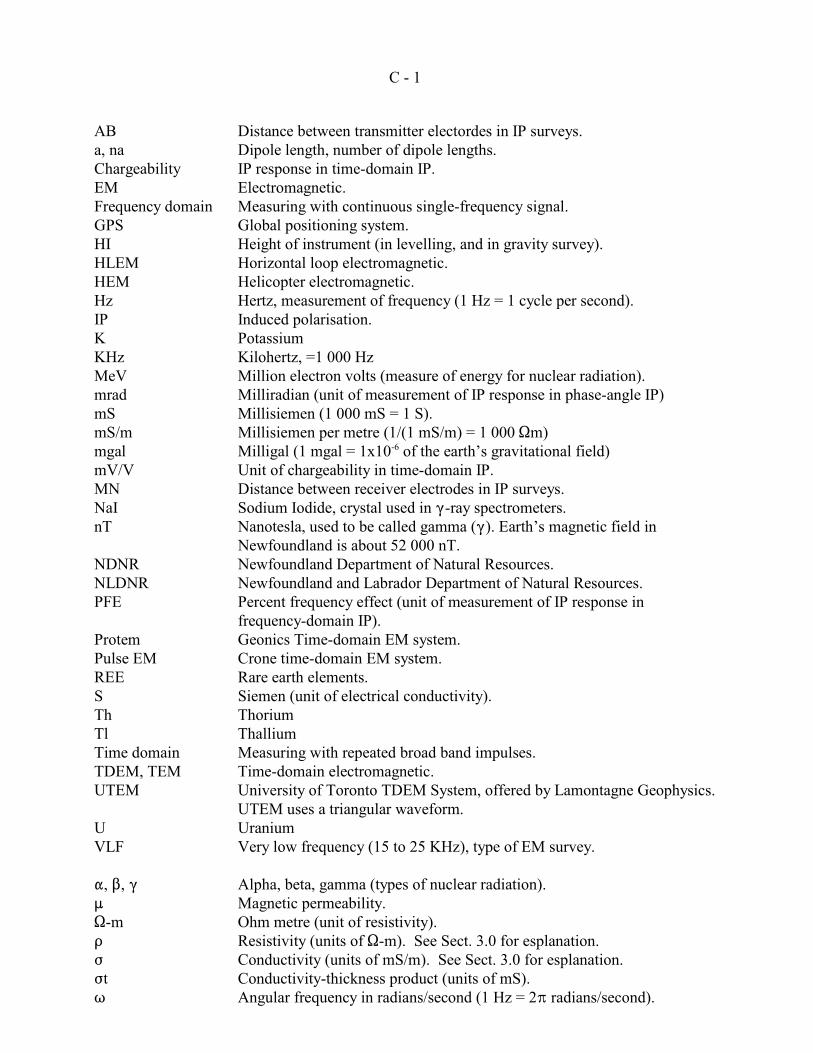
Appendix C:

List of Acronyms, Symbols and Terms

C - 1

AB Distance between transmitter electordes in IP surveys.a, na Dipole length, number of dipole lengths.Chargeability IP response in time-domain IP.EM Electromagnetic.Frequency domain Measuring with continuous single-frequency signal.GPS Global positioning system.HI Height of instrument (in levelling, and in gravity survey).HLEM Horizontal loop electromagnetic.HEM Helicopter electromagnetic.Hz Hertz, measurement of frequency (1 Hz = 1 cycle per second).IP Induced polarisation.K PotassiumKHz Kilohertz, =1 000 HzMeV Million electron volts (measure of energy for nuclear radiation).mrad Milliradian (unit of measurement of IP response in phase-angle IP)mS Millisiemen (1 000 mS = 1 S).mS/m Millisiemen per metre (1/(1 mS/m) = 1 000 Sm)mgal Milligal (1 mgal = 1x10 of the earth’s gravitational field)-6

mV/V Unit of chargeability in time-domain IP.MN Distance between receiver electrodes in IP surveys.NaI Sodium Iodide, crystal used in (-ray spectrometers.nT Nanotesla, used to be called gamma ((). Earth’s magnetic field in

Newfoundland is about 52 000 nT.NDNR Newfoundland Department of Natural Resources.NLDNR Newfoundland and Labrador Department of Natural Resources.PFE Percent frequency effect (unit of measurement of IP response in

frequency-domain IP).Protem Geonics Time-domain EM system.Pulse EM Crone time-domain EM system.REE Rare earth elements.S Siemen (unit of electrical conductivity).Th ThoriumTl ThalliumTime domain Measuring with repeated broad band impulses.TDEM, TEM Time-domain electromagnetic.UTEM University of Toronto TDEM System, offered by Lamontagne Geophysics.

UTEM uses a triangular waveform.U UraniumVLF Very low frequency (15 to 25 KHz), type of EM survey.

", $, ( Alpha, beta, gamma (types of nuclear radiation).: Magnetic permeability.S-m Ohm metre (unit of resistivity).D Resistivity (units of S-m). See Sect. 3.0 for esplanation.F Conductivity (units of mS/m). See Sect. 3.0 for esplanation. Ft Conductivity-thickness product (units of mS).T Angular frequency in radians/second (1 Hz = 2B radians/second).