Georeferencing Quick ReferenceGuide

Paula F. Zermoglio, Arthur D. Chapman, John R. Wieczorek, María Celeste Luna,David A. Bloom

Version 7adb86d, 2021-02-01 17:30:10 UTC

Table of ContentsColophon. . . . . . . . . . . . . . . . . . . . . . . . . . . . . . . . . . . . . . . . . . . . . . . . . . . . . . . . . . . . . . . . . . . . . . . . . . . . . . . .  1

Suggested citation. . . . . . . . . . . . . . . . . . . . . . . . . . . . . . . . . . . . . . . . . . . . . . . . . . . . . . . . . . . . . . . . . . . . . .  1Authors . . . . . . . . . . . . . . . . . . . . . . . . . . . . . . . . . . . . . . . . . . . . . . . . . . . . . . . . . . . . . . . . . . . . . . . . . . . . . . .  1Contributors . . . . . . . . . . . . . . . . . . . . . . . . . . . . . . . . . . . . . . . . . . . . . . . . . . . . . . . . . . . . . . . . . . . . . . . . . . .  1Licence . . . . . . . . . . . . . . . . . . . . . . . . . . . . . . . . . . . . . . . . . . . . . . . . . . . . . . . . . . . . . . . . . . . . . . . . . . . . . . .  1Disclaimer . . . . . . . . . . . . . . . . . . . . . . . . . . . . . . . . . . . . . . . . . . . . . . . . . . . . . . . . . . . . . . . . . . . . . . . . . . . . .  1Persistent URI . . . . . . . . . . . . . . . . . . . . . . . . . . . . . . . . . . . . . . . . . . . . . . . . . . . . . . . . . . . . . . . . . . . . . . . . .  1Document control . . . . . . . . . . . . . . . . . . . . . . . . . . . . . . . . . . . . . . . . . . . . . . . . . . . . . . . . . . . . . . . . . . . . . .  1Cover image . . . . . . . . . . . . . . . . . . . . . . . . . . . . . . . . . . . . . . . . . . . . . . . . . . . . . . . . . . . . . . . . . . . . . . . . . . .  1

1. Introduction . . . . . . . . . . . . . . . . . . . . . . . . . . . . . . . . . . . . . . . . . . . . . . . . . . . . . . . . . . . . . . . . . . . . . . . . . . .  21.1. Objectives . . . . . . . . . . . . . . . . . . . . . . . . . . . . . . . . . . . . . . . . . . . . . . . . . . . . . . . . . . . . . . . . . . . . . . . . .  21.2. Target Audience . . . . . . . . . . . . . . . . . . . . . . . . . . . . . . . . . . . . . . . . . . . . . . . . . . . . . . . . . . . . . . . . . . . .  21.3. Scope . . . . . . . . . . . . . . . . . . . . . . . . . . . . . . . . . . . . . . . . . . . . . . . . . . . . . . . . . . . . . . . . . . . . . . . . . . . . .  21.4. Changes from Previous Version . . . . . . . . . . . . . . . . . . . . . . . . . . . . . . . . . . . . . . . . . . . . . . . . . . . . . .  31.5. Using Darwin Core . . . . . . . . . . . . . . . . . . . . . . . . . . . . . . . . . . . . . . . . . . . . . . . . . . . . . . . . . . . . . . . . . .  31.6. Georeferencing Concepts . . . . . . . . . . . . . . . . . . . . . . . . . . . . . . . . . . . . . . . . . . . . . . . . . . . . . . . . . . . .  5

1.6.1. Locality Type . . . . . . . . . . . . . . . . . . . . . . . . . . . . . . . . . . . . . . . . . . . . . . . . . . . . . . . . . . . . . . . . . . .  51.6.2. Corrected Center . . . . . . . . . . . . . . . . . . . . . . . . . . . . . . . . . . . . . . . . . . . . . . . . . . . . . . . . . . . . . . .  51.6.3. Radial of Feature. . . . . . . . . . . . . . . . . . . . . . . . . . . . . . . . . . . . . . . . . . . . . . . . . . . . . . . . . . . . . . . .  61.6.4. Latitude . . . . . . . . . . . . . . . . . . . . . . . . . . . . . . . . . . . . . . . . . . . . . . . . . . . . . . . . . . . . . . . . . . . . . . .  61.6.5. Longitude. . . . . . . . . . . . . . . . . . . . . . . . . . . . . . . . . . . . . . . . . . . . . . . . . . . . . . . . . . . . . . . . . . . . . .  71.6.6. Coordinate Source . . . . . . . . . . . . . . . . . . . . . . . . . . . . . . . . . . . . . . . . . . . . . . . . . . . . . . . . . . . . . .  71.6.7. Coordinate Format . . . . . . . . . . . . . . . . . . . . . . . . . . . . . . . . . . . . . . . . . . . . . . . . . . . . . . . . . . . . . .  71.6.8. Coordinate Precision . . . . . . . . . . . . . . . . . . . . . . . . . . . . . . . . . . . . . . . . . . . . . . . . . . . . . . . . . . . .  81.6.9. Datum. . . . . . . . . . . . . . . . . . . . . . . . . . . . . . . . . . . . . . . . . . . . . . . . . . . . . . . . . . . . . . . . . . . . . . . . .  91.6.10. Direction . . . . . . . . . . . . . . . . . . . . . . . . . . . . . . . . . . . . . . . . . . . . . . . . . . . . . . . . . . . . . . . . . . . . .  91.6.11. Offset Distance . . . . . . . . . . . . . . . . . . . . . . . . . . . . . . . . . . . . . . . . . . . . . . . . . . . . . . . . . . . . . . . .  91.6.12. Distance Units . . . . . . . . . . . . . . . . . . . . . . . . . . . . . . . . . . . . . . . . . . . . . . . . . . . . . . . . . . . . . . . .  101.6.13. Distance Precision . . . . . . . . . . . . . . . . . . . . . . . . . . . . . . . . . . . . . . . . . . . . . . . . . . . . . . . . . . . .  101.6.14. Measurement Error . . . . . . . . . . . . . . . . . . . . . . . . . . . . . . . . . . . . . . . . . . . . . . . . . . . . . . . . . . .  101.6.15. GPS Accuracy. . . . . . . . . . . . . . . . . . . . . . . . . . . . . . . . . . . . . . . . . . . . . . . . . . . . . . . . . . . . . . . . .  111.6.16. Uncertainty . . . . . . . . . . . . . . . . . . . . . . . . . . . . . . . . . . . . . . . . . . . . . . . . . . . . . . . . . . . . . . . . . .  11

2. Georeferencing Methods by Locality Type . . . . . . . . . . . . . . . . . . . . . . . . . . . . . . . . . . . . . . . . . . . . . . . .  112.1. Geographic Feature only . . . . . . . . . . . . . . . . . . . . . . . . . . . . . . . . . . . . . . . . . . . . . . . . . . . . . . . . . . .  11

2.1.1. Feature – with Obvious Spatial Extent. . . . . . . . . . . . . . . . . . . . . . . . . . . . . . . . . . . . . . . . . . . . .  122.1.2. Feature – without Obvious Spatial Extent. . . . . . . . . . . . . . . . . . . . . . . . . . . . . . . . . . . . . . . . . .  132.1.3. Feature – Special Cases . . . . . . . . . . . . . . . . . . . . . . . . . . . . . . . . . . . . . . . . . . . . . . . . . . . . . . . . .  15

2.1.3.1. Feature – Street Address . . . . . . . . . . . . . . . . . . . . . . . . . . . . . . . . . . . . . . . . . . . . . . . . . . . .  15

2.1.3.2. Feature – Property . . . . . . . . . . . . . . . . . . . . . . . . . . . . . . . . . . . . . . . . . . . . . . . . . . . . . . . . .  172.1.3.3. Feature – Path . . . . . . . . . . . . . . . . . . . . . . . . . . . . . . . . . . . . . . . . . . . . . . . . . . . . . . . . . . . . .  182.1.3.4. Feature – Junction, Intersection, Crossing, Confluence . . . . . . . . . . . . . . . . . . . . . . . . . .  202.1.3.5. Feature – Cave . . . . . . . . . . . . . . . . . . . . . . . . . . . . . . . . . . . . . . . . . . . . . . . . . . . . . . . . . . . . .  212.1.3.6. Feature – Dive Location . . . . . . . . . . . . . . . . . . . . . . . . . . . . . . . . . . . . . . . . . . . . . . . . . . . . .  222.1.3.7. Feature – Headwaters of a Waterway . . . . . . . . . . . . . . . . . . . . . . . . . . . . . . . . . . . . . . . . .  232.1.3.8. Feature – near a Feature . . . . . . . . . . . . . . . . . . . . . . . . . . . . . . . . . . . . . . . . . . . . . . . . . . . .  242.1.3.9. Feature – between Two Features . . . . . . . . . . . . . . . . . . . . . . . . . . . . . . . . . . . . . . . . . . . . .  262.1.3.10. Feature – between Two Paths. . . . . . . . . . . . . . . . . . . . . . . . . . . . . . . . . . . . . . . . . . . . . . .  27

2.2. Offsets . . . . . . . . . . . . . . . . . . . . . . . . . . . . . . . . . . . . . . . . . . . . . . . . . . . . . . . . . . . . . . . . . . . . . . . . . . .  282.2.1. Offset – Distance only . . . . . . . . . . . . . . . . . . . . . . . . . . . . . . . . . . . . . . . . . . . . . . . . . . . . . . . . . .  282.2.2. Offset – Heading only . . . . . . . . . . . . . . . . . . . . . . . . . . . . . . . . . . . . . . . . . . . . . . . . . . . . . . . . . .  292.2.3. Offset – Distance along a Path . . . . . . . . . . . . . . . . . . . . . . . . . . . . . . . . . . . . . . . . . . . . . . . . . . .  30

2.2.3.1. Offset along a Narrow Path. . . . . . . . . . . . . . . . . . . . . . . . . . . . . . . . . . . . . . . . . . . . . . . . . .  322.2.3.2. Offset along a Wide Path . . . . . . . . . . . . . . . . . . . . . . . . . . . . . . . . . . . . . . . . . . . . . . . . . . . .  332.2.3.3. Offset along Multiple Possible Paths . . . . . . . . . . . . . . . . . . . . . . . . . . . . . . . . . . . . . . . . . .  34

2.2.4. Offset – Distance along Orthogonal Directions. . . . . . . . . . . . . . . . . . . . . . . . . . . . . . . . . . . . .  352.2.5. Offset – Distance at a Heading. . . . . . . . . . . . . . . . . . . . . . . . . . . . . . . . . . . . . . . . . . . . . . . . . . .  362.2.6. Offset – Distances from Two Distinct Paths . . . . . . . . . . . . . . . . . . . . . . . . . . . . . . . . . . . . . . . .  37

2.3. Coordinates. . . . . . . . . . . . . . . . . . . . . . . . . . . . . . . . . . . . . . . . . . . . . . . . . . . . . . . . . . . . . . . . . . . . . . .  382.3.1. Coordinates – Geographic Coordinates . . . . . . . . . . . . . . . . . . . . . . . . . . . . . . . . . . . . . . . . . . .  382.3.2. Coordinates – Universal Transverse Mercator (UTM) . . . . . . . . . . . . . . . . . . . . . . . . . . . . . . . .  392.3.3. Coordinates – Grid Systems . . . . . . . . . . . . . . . . . . . . . . . . . . . . . . . . . . . . . . . . . . . . . . . . . . . . .  40

2.4. Difficult Localities. . . . . . . . . . . . . . . . . . . . . . . . . . . . . . . . . . . . . . . . . . . . . . . . . . . . . . . . . . . . . . . . . .  412.4.1. Dubious Locations . . . . . . . . . . . . . . . . . . . . . . . . . . . . . . . . . . . . . . . . . . . . . . . . . . . . . . . . . . . . .  412.4.2. Cannot Be Located . . . . . . . . . . . . . . . . . . . . . . . . . . . . . . . . . . . . . . . . . . . . . . . . . . . . . . . . . . . . .  412.4.3. More than One Matching Feature . . . . . . . . . . . . . . . . . . . . . . . . . . . . . . . . . . . . . . . . . . . . . . . .  42

2.4.3.1. Multiple Related Nearby Features . . . . . . . . . . . . . . . . . . . . . . . . . . . . . . . . . . . . . . . . . . . .  422.4.3.2. Multiple Unrelated Features . . . . . . . . . . . . . . . . . . . . . . . . . . . . . . . . . . . . . . . . . . . . . . . . .  43

2.4.4. Demonstrably Inconsistent. . . . . . . . . . . . . . . . . . . . . . . . . . . . . . . . . . . . . . . . . . . . . . . . . . . . . .  432.4.5. Cultivated or Captive . . . . . . . . . . . . . . . . . . . . . . . . . . . . . . . . . . . . . . . . . . . . . . . . . . . . . . . . . . .  44

Glossary. . . . . . . . . . . . . . . . . . . . . . . . . . . . . . . . . . . . . . . . . . . . . . . . . . . . . . . . . . . . . . . . . . . . . . . . . . . . . . . .  45Acknowledgements. . . . . . . . . . . . . . . . . . . . . . . . . . . . . . . . . . . . . . . . . . . . . . . . . . . . . . . . . . . . . . . . . . . . . .  52References . . . . . . . . . . . . . . . . . . . . . . . . . . . . . . . . . . . . . . . . . . . . . . . . . . . . . . . . . . . . . . . . . . . . . . . . . . . . .  52Appendix A: Key to Locality Types. . . . . . . . . . . . . . . . . . . . . . . . . . . . . . . . . . . . . . . . . . . . . . . . . . . . . . . . . .  54

Features . . . . . . . . . . . . . . . . . . . . . . . . . . . . . . . . . . . . . . . . . . . . . . . . . . . . . . . . . . . . . . . . . . . . . . . . . . . . .  54Offsets. . . . . . . . . . . . . . . . . . . . . . . . . . . . . . . . . . . . . . . . . . . . . . . . . . . . . . . . . . . . . . . . . . . . . . . . . . . . . . .  55Coordinates . . . . . . . . . . . . . . . . . . . . . . . . . . . . . . . . . . . . . . . . . . . . . . . . . . . . . . . . . . . . . . . . . . . . . . . . . .  56Difficult Localities . . . . . . . . . . . . . . . . . . . . . . . . . . . . . . . . . . . . . . . . . . . . . . . . . . . . . . . . . . . . . . . . . . . . .  57

Appendix B: Methods to Find the Corrected Center and Geographic Radial . . . . . . . . . . . . . . . . . . . . . .  58Introduction . . . . . . . . . . . . . . . . . . . . . . . . . . . . . . . . . . . . . . . . . . . . . . . . . . . . . . . . . . . . . . . . . . . . . . . . . .  58

Linear Feature . . . . . . . . . . . . . . . . . . . . . . . . . . . . . . . . . . . . . . . . . . . . . . . . . . . . . . . . . . . . . . . . . . . . . .  59Elongate Convex Feature. . . . . . . . . . . . . . . . . . . . . . . . . . . . . . . . . . . . . . . . . . . . . . . . . . . . . . . . . . . . .  59Not Obviously Elongate Convex Feature. . . . . . . . . . . . . . . . . . . . . . . . . . . . . . . . . . . . . . . . . . . . . . . .  59Simple Concave Feature (center within the feature) . . . . . . . . . . . . . . . . . . . . . . . . . . . . . . . . . . . . . .  60Complex Concave Feature (center outside the feature) . . . . . . . . . . . . . . . . . . . . . . . . . . . . . . . . . . .  60Curvilinear Feature . . . . . . . . . . . . . . . . . . . . . . . . . . . . . . . . . . . . . . . . . . . . . . . . . . . . . . . . . . . . . . . . . .  61

Colophon

Suggested citationZermoglio PF, Chapman AD, Wieczorek JR, Luna MC & Bloom DA (2020) Georeferencing QuickReference Guide. Copenhagen: GBIF Secretariat. https://doi.org/10.35035/e09p-h128

AuthorsPaula F. Zermoglio, Arthur D. Chapman, John R. Wieczorek, Marie Celeste Luna & David A. Bloom

Contributors

LicenceThe document Georeferencing Quick Reference Guide is licensed under Creative Commons Attribution-ShareAlike 4.0 Unported License.

DisclaimerThe information in this book represents the professional opinion of the authors, and does notnecessarily represent the views of the publisher. While the authors and the publisher haveattempted to make this book as accurate and as thorough as possible, the information containedherein is provided on an "As Is" basis, and without any warranties with respect to its accuracy orcompleteness. The authors and the publisher shall have no liability to any person or entity for anyloss or damage caused by using the information provided in this book.

Where there are differences in interpretation between this document and translated versions inlanguages other than English, the English version remains the original and definitive version.

Persistent URIhttps://doi.org/10.35035/e09p-h128

Document controlv1.0, December 2020

Cover imageCommerson’s dolphin (Cephalorhynchus commersonii), off the coast of Chubut, Argentina. Photo 2018Gabriel Laufer via iNaturalist research-grade observations, in the public domain under CC0.

1

1. IntroductionThis is a practical guide for georeferencing. It describes the protocols to determine the shapes offeatures and how to use them as the basis for georeferencing with the point-radius georeferencingmethod (Wieczorek 2001, Wieczorek et al. 2004, Chapman & Wieczorek 2020) using theGeoreferencing Calculator (Wieczorek & Wieczorek 2020), and its associated GeoreferencingCalculator Manual (Bloom et al. 2020), maps, gazetteers, and other resources from whichcoordinates and spatial boundaries for places can be found. This document is a citablegeoreferencing protocol. If a derived protocol is used, a new document with attribution to this Guideshould be made publicly available and cited.

This Guide is based on a first version of the Guide (Wieczorek et al. 2012)), which was in turn anadaptation of Georeferencing for Dummies (Spencer et al. 2008). It explains the recommendedgeoreferencing procedures for the most commonly encountered type of localities. This Guide shouldbe used in parallel with the Georeferencing Best Practices (Chapman & Wieczorek 2020), whichcontains the theoretical background and more detailed information about concepts used here.

Underlined terms throughout this document (e.g. accuracy) link to definitions in the Glossary. Termsin italics (e.g. Input Latitude) refer to fields and/or labels in the Georeferencing Calculator (Wieczorek& Wieczorek 2020) (hereafter referred to as 'the Calculator'). Darwin Core terms are displayed inmonospace (e.g. dwc:georeferenceRemarks) in all GBIF digital documentation.

At the end of this document is a Georeference Quick Reference Guide Key to Locality Types, whichcontains a quick summary of the protocols for the most common locality types, described in detail inthe sections of this guide.

1.1. ObjectivesThis document provides guidance on how to georeference using the point-radius method. ThisGuide also provides the methods for determining the boundaries of features, which form the basisof the shape georeferencing method.

1.2. Target AudienceThis document is a practical guide for anyone who needs to georeference textual localitydescriptions so that they can be used in spatial filtering or analysis in research, education, or themaintenance of biological collections data.

1.3. ScopeThis document is one of three that cover recommended requirements and methods to georeferencelocations. It provides a practical how-to guide for putting the theory of the point-radiusgeoreferencing method into practice.

The Guide relies on the Georeferencing Best Practices (Chapman & Wieczorek 2020) forbackground, definitions, and more detailed explanations of the theory behind the methods andcalculations found here and in the Calculator.

2

The third document is the Georeferencing Calculator Manual (Bloom et al. 2020), which describeshow to use the Georeferencing Calculator. The Calculator is a browser-based JavaScript applicationthat aids in georeferencing descriptive localities, and making the calculations necessary to obtaingeographic coordinates and uncertainties for locations using the point-radius method.

These documents DO NOT provide guidance on georectifying images or geocoding street addresses– distinct operations that are sometimes called "georeferencing".

1.4. Changes from Previous VersionThis version of the Guide is a complete remake of its previous edition, reorganized and augmentedto include graphical examples of each type of location and detailed steps for how to georeferencethem. There have been a few changes in terminology since the previous edition, which include:

• Extent in the previous version has been changed to radial. Extent, where retained, is used in amore traditional way to mean the entire space within a location.

• "Named place" has been replaced with feature.

• Where the geographic center was recommended in the past, corrected center based on thegeographic radial is now used. This is an important change because the geographic center didnot necessarily yield the smallest uncertainty due to the extent of a feature; the corrected centerand geographic radial does.

1.5. Using Darwin CoreGeoreferences using the methods in this Guide will be of greatest value if as much information aspossible is captured about and during the georeferencing process. The Darwin Core standard(Darwin Core Maintenance Group 2020) defines all of the fields recommended for the capture ofreproducible georeferences, as follows:

Darwin Core georeferencing terms:

dwc:decimalLatitude, dwc:decimalLongitude, dwc:geodeticDatum

the combination of these fields provide the reference for the center of the point-radiusrepresentation of the georeference.

dwc:coordinateUncertaintyInMeters

The horizontal distance in meters from the given decimalLatitude and decimalLongitude thatdescribes the smallest enclosing circle that contains the whole of the location. Leave the valueempty if the uncertainty is unknown, cannot be estimated, or is not applicable (because there areno coordinates). Zero is not a valid value for this term. This term corresponds with the geographicradial of the final georeference.

dwc:georeferencedBy, dwc:georeferencedDate

the individual(s) who last modified the georeference and when that happened. These correspondto the final authority on the georeference in its current state, regardless of who might haveworked on previous versions of the georeference.

3

dwc:georeferenceProtocol

A description or reference to the methods used to determine the shape using the shapegeoreferencing method, or the coordinates and uncertainty using the point-radius method. If theprotocol in this Guide is used unaltered, then the georeferenceProtocol should be the citation forthis document.

dwc:georeferenceSources

A list (concatenated and separated) of maps, gazetteers, or other resources used to georeferencethe location, described specifically enough to allow anyone in the future to use the sameresources.

Examples

USGS 1:24000 Florence Montana Quad 1967Terrametrics 2008 Google EarthWieczorek C & J Wieczorek (2020) Georeferencing Calculator, version yyyymmdd. Available:http://georeferencing.org/georefcalculator/gc.html.

dwc:georeferenceVerificationStatus

A categorical description of the extent to which the georeference has been verified to representthe best possible spatial description. Recommended best practice is to use a controlledvocabulary. Note that this verification could only be performed in relation to the occurrence orevent that is being recorded.

Examples

requires verificationverified by collectorverified by curator

dwc:georeferenceRemarks

Notes or comments out of the ordinary about the georeference, explaining assumptions made inaddition or opposition to those formalized in the method referred to in georeferenceProtocol.

Example

assumed distance by road (Hwy. 101)

dwc:locationRemarks

Notes or comments of interest about the location (not the georeference of the location, which goin georeferenceRemarks).

Example

Villa Epecuen was inundated in November 1985 and ceased to be inhabited until 2009

4

For additional community discussion and recommendations, see the Darwin Core Questions &Answers Site, the Darwin Core Hour Webinars and Georeferencing Best Practices (Chapman &Wieczorek 2020).

1.6. Georeferencing ConceptsOne of the goals of georeferencing following best practices is to be sure that enough information isprovided in the output so that the georeference is repeatable (see Principles of Best Practice inGeoreferencing Best Practices (Chapman & Wieczorek 2020)). To that end, this document provides aset of recipes for georeferencing various locality types using the Georeferencing Calculator. TheCalculator allows you to make distinct kinds of calculations based on the locality type (§ 1.6.1). Whenthe locality type is chosen from the predefined list, the Calculator presents input boxes for all of theparameters needed for that type of calculation. Note that the locality type is for the most specificclause in the locality description (see Parsing the Locality Description in Georeferencing BestPractices (Chapman & Wieczorek 2020)). However, there may be information for other clauses orother parts of the location record that help to constrain the location and come into play when afeature boundary is determined. Many Calculator parameters are used for more than one localitytype. Rather than repeat the explanation for each locality type, they are collected here for commonreference. Some locality types require specific parameters, for which the corresponding explanationsare included in each subsection of § 2. Refer to the Georeferencing Calculator Manual (Bloom et al.2020) for details about the Calculator not answered in this document.

1.6.1. Locality Type

The locality type refers to the pattern of the most specific part of a locality description to begeoreferenced – the one that determines which calculation method to use. The Calculator hasoptions to compute georeferences for six basic locality types:

• Coordinates only

• Geographic feature only

• Distance only

• Distance along a path

• Distance along orthogonal directions

• Distance at a heading

Selecting a locality type will configure the Calculator to show all of the parameters that need to beset to perform the georeference calculation. This Guide gives specific instructions for how to set theparameters for many different examples of each of the locality types.

1.6.2. Corrected Center

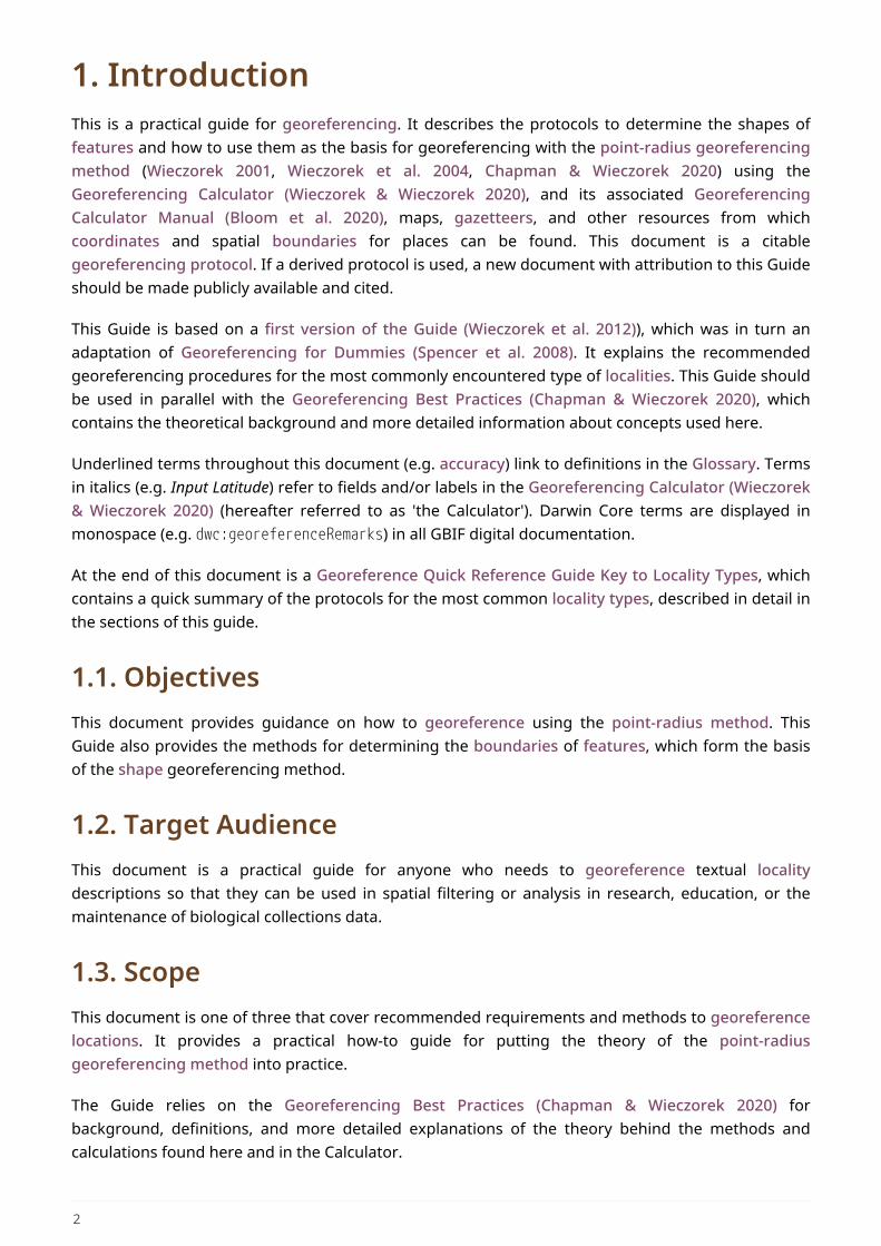
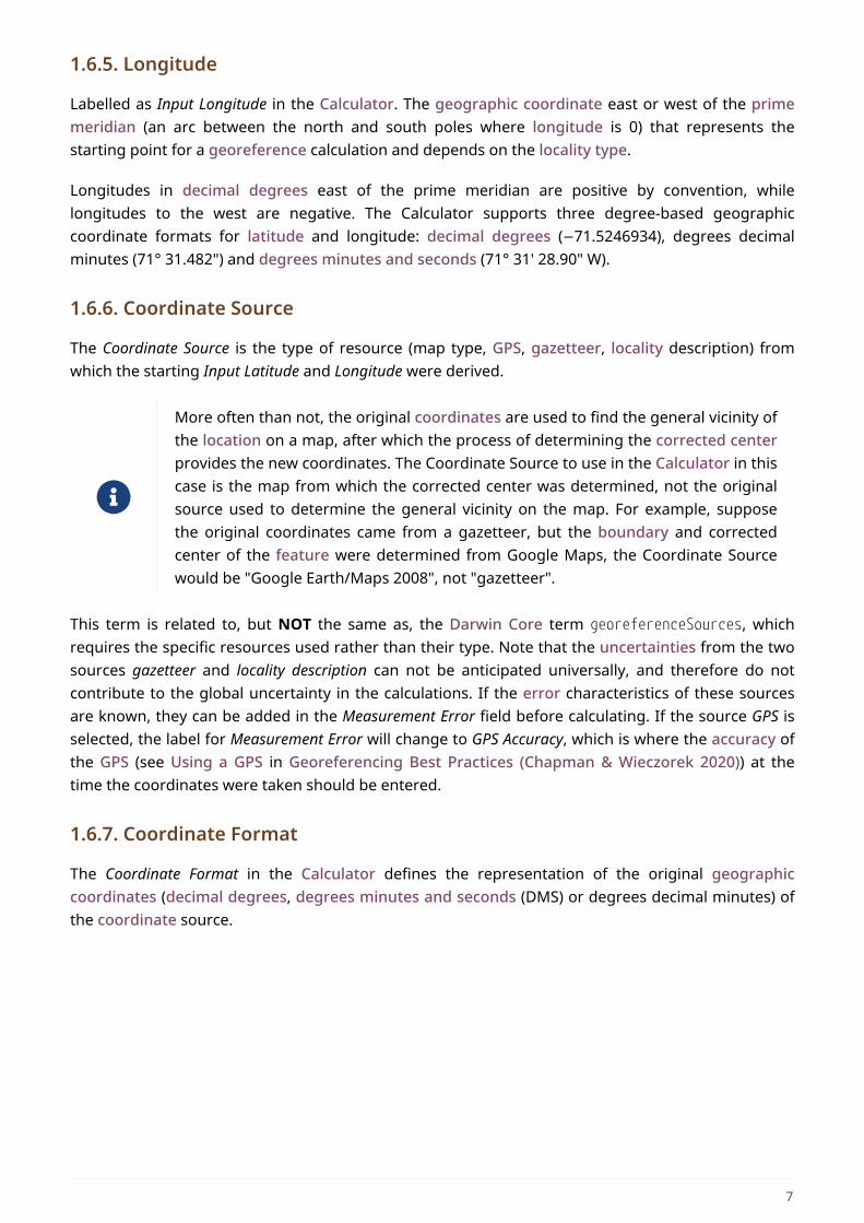
The corrected center is the point within a location, or on its boundary, that minimizes thegeographic radial (see § 1.6.3). This point is obtained by finding the smallest enclosing circle thatcontains the entire feature, and then taking the center of that circle (Figure 1A). If that center doesnot fall on or inside the boundaries of the feature, find the smallest enclosing circle that contains theentire feature, but has its center on the boundary of the feature (Figure 1B). Note that in the

5

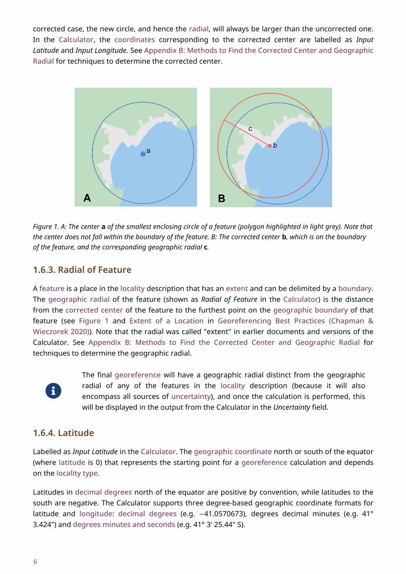
corrected case, the new circle, and hence the radial, will always be larger than the uncorrected one.In the Calculator, the coordinates corresponding to the corrected center are labelled as InputLatitude and Input Longitude. See Appendix B: Methods to Find the Corrected Center and GeographicRadial for techniques to determine the corrected center.

Figure 1. A: The center a of the smallest enclosing circle of a feature (polygon highlighted in light grey). Note thatthe center does not fall within the boundary of the feature. B: The corrected center b, which is on the boundaryof the feature, and the corresponding geographic radial c.

1.6.3. Radial of Feature

A feature is a place in the locality description that has an extent and can be delimited by a boundary.The geographic radial of the feature (shown as Radial of Feature in the Calculator) is the distancefrom the corrected center of the feature to the furthest point on the geographic boundary of thatfeature (see Figure 1 and Extent of a Location in Georeferencing Best Practices (Chapman &Wieczorek 2020)). Note that the radial was called "extent" in earlier documents and versions of theCalculator. See Appendix B: Methods to Find the Corrected Center and Geographic Radial fortechniques to determine the geographic radial.

The final georeference will have a geographic radial distinct from the geographicradial of any of the features in the locality description (because it will alsoencompass all sources of uncertainty), and once the calculation is performed, thiswill be displayed in the output from the Calculator in the Uncertainty field.

1.6.4. Latitude

Labelled as Input Latitude in the Calculator. The geographic coordinate north or south of the equator(where latitude is 0) that represents the starting point for a georeference calculation and dependson the locality type.

Latitudes in decimal degrees north of the equator are positive by convention, while latitudes to thesouth are negative. The Calculator supports three degree-based geographic coordinate formats forlatitude and longitude: decimal degrees (e.g. −41.0570673), degrees decimal minutes (e.g. 41°3.424") and degrees minutes and seconds (e.g. 41° 3' 25.44" S).

6

1.6.5. Longitude

Labelled as Input Longitude in the Calculator. The geographic coordinate east or west of the primemeridian (an arc between the north and south poles where longitude is 0) that represents thestarting point for a georeference calculation and depends on the locality type.

Longitudes in decimal degrees east of the prime meridian are positive by convention, whilelongitudes to the west are negative. The Calculator supports three degree-based geographiccoordinate formats for latitude and longitude: decimal degrees (−71.5246934), degrees decimalminutes (71° 31.482") and degrees minutes and seconds (71° 31' 28.90" W).

1.6.6. Coordinate Source

The Coordinate Source is the type of resource (map type, GPS, gazetteer, locality description) fromwhich the starting Input Latitude and Longitude were derived.

More often than not, the original coordinates are used to find the general vicinity ofthe location on a map, after which the process of determining the corrected centerprovides the new coordinates. The Coordinate Source to use in the Calculator in thiscase is the map from which the corrected center was determined, not the originalsource used to determine the general vicinity on the map. For example, supposethe original coordinates came from a gazetteer, but the boundary and correctedcenter of the feature were determined from Google Maps, the Coordinate Sourcewould be "Google Earth/Maps 2008", not "gazetteer".

This term is related to, but NOT the same as, the Darwin Core term georeferenceSources, whichrequires the specific resources used rather than their type. Note that the uncertainties from the twosources gazetteer and locality description can not be anticipated universally, and therefore do notcontribute to the global uncertainty in the calculations. If the error characteristics of these sourcesare known, they can be added in the Measurement Error field before calculating. If the source GPS isselected, the label for Measurement Error will change to GPS Accuracy, which is where the accuracy ofthe GPS (see Using a GPS in Georeferencing Best Practices (Chapman & Wieczorek 2020)) at thetime the coordinates were taken should be entered.

1.6.7. Coordinate Format

The Coordinate Format in the Calculator defines the representation of the original geographiccoordinates (decimal degrees, degrees minutes and seconds (DMS) or degrees decimal minutes) ofthe coordinate source.

7

When the calculation type is not “Coordinates only”, the original coordinates areoften used to find the general vicinity of the location on a map, after which theprocess of determining the corrected center provides the new coordinates. TheCoordinate Format to use in the Calculator in this case is the coordinate format onthe map from which the corrected center was determined, not the coordinateformat of the original source used to determine the general vicinity on the map. Forexample, suppose the original coordinates came from a gazetteer in DMS, but theboundary and corrected center of the feature were determined from Google Maps,the Coordinate Format would be decimal degrees, not DMS.

This term is only equivalent to the Darwin Core term verbatimCoordinateSystem if no conversionshad to be performed from the original source to the format used in the Input Latitude and InputLongitude (e.g. if the original coordinates were UTM and you had to convert them to DMS, then theCoordinate Format in the Calculator will be DMS, but the verbatimCoordinateSystem will be UTM.Selecting the original coordinate format allows the coordinates to be entered in their native formatand forces the Calculator to present appropriate options for coordinate precision. Changing thecoordinate format will automatically reset the coordinate precision value to nearest degree. Be sure tocorrect this for the actual coordinate precision. The Calculator stores coordinates in decimal degreesto seven decimal places. This is to preserve the correct coordinates in all formats regardless of howmany coordinate transformations are done.

1.6.8. Coordinate Precision

Labelled in the Calculator as Precision in the first column of input parameters, this drop-down list ispopulated with levels of precision in keeping with the coordinate format chosen. For example, with aCoordinate Format of degrees minutes seconds, an Input Latitude of 35° 22' 24" N and an InputLongitude of 105° 22' 28" W, the Coordinate Precision would be nearest second. A value of exact is anylevel of precision higher than the otherwise highest precision given on the list. Sources of coordinateprecision may include paper or digital maps, digital imagery, GPS, gazetteers, or localitydescriptions.

The Coordinate Precision to use in the Calculator is the coordinate precision of thesource from which the corrected center was determined, not the coordinateprecision of the original source used to determine the general vicinity on the map.For example, suppose the original coordinates came from a gazetteer, but theboundary and corrected center of the feature were determined from Google Maps,the Coordinate Precision would be determined by the number of digits of decimaldegrees you captured from the corrected center on Google Maps, not theCoordinate Precision of the coordinates from the original gazetteer entry. If you useall of the digits provided on Google Maps, the Coordinate Precision would be"exact".

This term is similar to, but NOT the same as, the Darwin Core termcoordinatePrecision, which applies to the output coordinates.

8

1.6.9. Datum

Defines the position of the origin and orientation of an ellipsoid upon which the coordinates arebased for the given Input Latitude and Longitude (see coordinate reference system).

The Datum to use in the Calculator is the datum (or ellipsoid) of the source fromwhich the corrected center was determined. For example, suppose the originalcoordinates came from a gazetteer with an unknown datum, but the boundary andcorrected center of the feature were determined from Google Maps, the Datumwould be "WGS84", not "datum not recorded."

The term Datum in the Calculator is equivalent to the Darwin Core term geodeticDatum. TheCalculator includes ellipsoids on the Datum drop-down list, as sometimes that is all that coordinatesource shows. The choice of datum in the Calculator has two important effects. The first is thecontribution to uncertainty if the datum of the input coordinates is not known. If the datum andellipsoid are not known, datum not recorded must be selected. Uncertainty due to an unknown datumcan be severe and varies geographically in a complex way, with a worst-case contribution of 5359 m(see Coordinate Reference System in Georeferencing Best Practices (Chapman & Wieczorek 2020)).The second important effect of the datum selection is to provide the characteristics of the ellipsoidmodel of the earth, on which the distance calculations depend.

1.6.10. Direction

The Direction in the Georeferencing Calculator is the heading given in the locality description, eitheras a standard compass point (see Boxing the compass) or as a number of degrees in the clockwisedirection from north. True North is not the same as Magnetic North (see Headings in GeoreferencingBest Practices (Chapman & Wieczorek 2020)). If a heading is known to be a magnetic heading, it willhave to be converted into a true heading (see NOAA’s Magnetic Field Calculator) before it can beused in the Calculator. If degrees from N is selected, a text box will appear to the right of theselection, into which the degree heading should be entered.

Some marine locality descriptions reference a direction (azimuth) toward alandmark rather than a heading from the current location (e.g. "327° to NubbleLighthouse"). To make a Distance a heading calculation for such a localitydescription, use the compass point 180 degrees from the one given in the localitydescription (147° in the example above) as the Direction.

1.6.11. Offset Distance

The Offset Distance in the Calculator is the linear surface distance from a point of origin. Offsets areused for the Locality Types Distance at a heading and Distance only. If the Locality Type Distance alongorthogonal directions is selected, there are two distinct offsets:

North or South Offset Distance

The distance to the north or south (set with the selection box to the right of the distance text box)of the Input Latitude.

9

East or West Offset Distance

The distance to the east or west (set with the selection box to the right of the distance text box) ofthe Input Longitude.

1.6.12. Distance Units

The Distance Units selection denotes the real world units used in the locality description. It isimportant to select the original units as given in the description. This is needed to incorporate theuncertainty from Distance Precision properly. If the locality description does not include distanceunits, use the distance units of the map from which measurements are derived.

Example 1.

• select mi for "10 mi E (by air) Bakersfield"

• select km for "3.2 km SE of Lisbon"

• select km for measurements in Google Maps where the distance units are set to km.

All distances used in a given calculation must use the same units. For example, if anoffset distance was given in miles in the locality description, when entering theradial value, you must do so in miles.

1.6.13. Distance Precision

The Distance Precision, labelled in the Calculator as Precision in the second column of inputparameters, refers to the precision with which a distance was described in a locality (see UncertaintyRelated to Offset Precision in Georeferencing Best Practices (Chapman & Wieczorek 2020)). Thisdrop-down list is populated based on the Distance Units chosen and contains powers of ten andsimple fractions to indicate the precision demonstrated in the verbatim original offset.

Example 2.

• select 1 mi for "6 mi NE of Davis"

• select ¼ km for "3.75 km W of Hamilton"

1.6.14. Measurement Error

The Measurement Error accounts for error associated with the ability to distinguish one point fromanother using any measuring tool, such as rulers on paper maps or the measuring tools on GoogleMaps or Google Earth. The units of measurement must be the same as those in the localitydescription as captured in Distance Units (see § 1.6.12). The Distance Converter at the bottom of theCalculator is provided to aid in changing a measurement to the locality description units. Forexample, a reasonable value for measurement error on a map is 1 mm, which on a map of 1:24,000scale would be 24 m.

10

1.6.15. GPS Accuracy

When GPS is selected from the Coordinate Source drop-down list, the label for the Measurement Errortext box changes to GPS Accuracy. We recommend entering a value that is at least twice the valuegiven by the GPS at the time the coordinates were captured (see Uncertainty due to GPS inGeoreferencing Best Practices (Chapman & Wieczorek 2020). If GPS Accuracy is not known, enter 100m for standard hand-held GPS coordinates taken before 1 May 2000 when Selective Availability wasdiscontinued. After that, use 30 m as a conservative default value.

1.6.16. Uncertainty

The Uncertainty in the Calculator is the calculated result of the combination of all sources ofuncertainty (coordinate precision, unknown datum, data source, GPS accuracy, measurement error,feature extent, distance precision and heading precision) expressed as a linear distance – thegeographic radial of the georeference and the radius in the point-radius method (Wieczorek et al.2004). Along with the Output Latitude, Output Longitude, and Datum, the radius defines a circlecontaining all of the possible places a locality description could mean. In the Calculator theUncertainty is given in meters.

2. Georeferencing Methods by Locality Type

2.1. Geographic Feature only

Definition

The simplest locality descriptions consist of only a named place, or more generally,a feature, which is often listed in a standard gazetteer and can probably be locatedon a map of the appropriate scale.

Despite how they might be presented in a gazetteer or on a map, features are not points; they areareas that have a spatial extent. Some features can have an obvious spatial extent, while others maynot. All variations of features are treated in this Guide as one or the other of these two maincategories. The basic methodology is to try to determine the boundaries of the feature, its correctedcenter and a measure of how specific the feature is (defined here by the geographic radial). SeeAppendix B: Methods to Find the Corrected Center and Geographic Radial for techniques todetermine the corrected center and geographic radial for various geometric types of features.

Coordinates from geographic indexes such as gazetteers often use reference pointsthat are not necessarily in the center of the feature. For example, a river may bereferenced by its mouth, and a town by its main post office, courthouse, or mainplaza. It is best to use a visual reference to determine boundaries, centers, andradials. For this reason, it is a good idea to use the gazetteer coordinates to find thefeature on a map, and then use the map to find the boundaries, corrected centerand geographic radial of the feature.

11

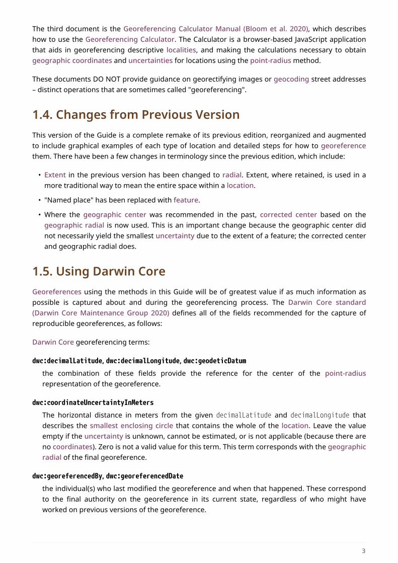
2.1.1. Feature – with Obvious Spatial Extent

The locality refers to a geographic feature with discernible spatial extent, i.e. the boundaries of thefeature can be determined easily (Figure 2).

Examples

• "Puerto Madryn"

• "Isla Tiburón"

• "Yosemite National Park"

• "Botany Bay"

Locality Type: Geographic feature only

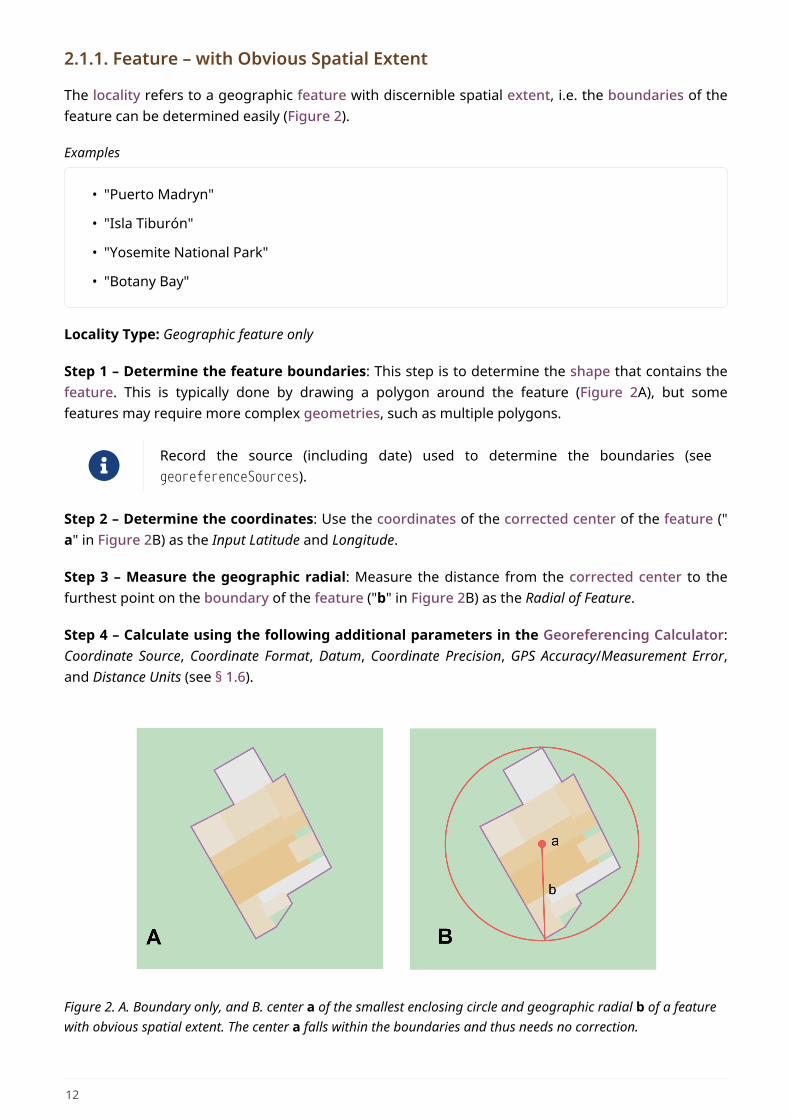
Step 1 – Determine the feature boundaries: This step is to determine the shape that contains thefeature. This is typically done by drawing a polygon around the feature (Figure 2A), but somefeatures may require more complex geometries, such as multiple polygons.

Record the source (including date) used to determine the boundaries (seegeoreferenceSources).

Step 2 – Determine the coordinates: Use the coordinates of the corrected center of the feature ("a" in Figure 2B) as the Input Latitude and Longitude.

Step 3 – Measure the geographic radial: Measure the distance from the corrected center to thefurthest point on the boundary of the feature ("b" in Figure 2B) as the Radial of Feature.

Step 4 – Calculate using the following additional parameters in the Georeferencing Calculator:Coordinate Source, Coordinate Format, Datum, Coordinate Precision, GPS Accuracy/Measurement Error,and Distance Units (see § 1.6).

Figure 2. A. Boundary only, and B. center a of the smallest enclosing circle and geographic radial b of a featurewith obvious spatial extent. The center a falls within the boundaries and thus needs no correction.

12

2.1.2. Feature – without Obvious Spatial Extent

The locality refers to a geographic feature that does not have an easily discernible spatial boundary.Some features may have undefined boundaries (e.g. mountains, unincorporated towns, etc.). Otherfeatures may only have a label, with no apparent boundaries or size on a map because they are smallor obscured on satellite imagery (e.g. spring, monument, etc.). Another possibility is a feature withonly coordinates from a gazetteer and no discernible presence on a map.

Examples

• "Pampa Grande" as a region

• "Mt Hypipamee"

• "Great Barrier Reef"

Locality Type: Geographic feature only

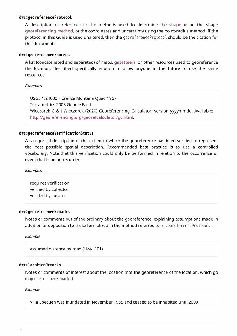
Step 1 – Estimate the feature boundaries: Determine the boundaries of the feature as well aspossible using visible evidence for the feature on a map. Try to get into the mind of the person whorecorded the locality. Imagine yourself there. What circumstances would influence which feature wasrecorded and what circumstances would have encouraged them to choose a different feature?

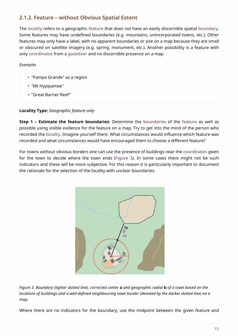
For towns without obvious borders one can use the presence of buildings near the coordinates givenfor the town to decide where the town ends (Figure 3). In some cases there might not be suchindicators and these will be more subjective. For this reason it is particularly important to documentthe rationale for the selection of the locality with unclear boundaries.

Figure 3. Boundary (lighter dotted line), corrected center a and geographic radial b of a town based on thelocations of buildings and a well-defined neighbouring town border (denoted by the darker dotted line) on amap.

Where there are no indicators for the boundary, use the midpoint between the given feature and

13

neighbouring features with similar type, size, or importance to make a rough boundary. Though thisboundary may not represent the actual feature very well, it will represent the uncertainty of wherethe locality is, and that is the major goal of the georeference.

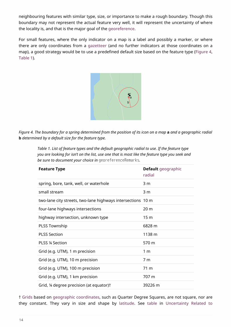
For small features, where the only indicator on a map is a label and possibly a marker, or wherethere are only coordinates from a gazetteer (and no further indicators at those coordinates on amap), a good strategy would be to use a predefined default size based on the feature type (Figure 4,Table 1).

Figure 4. The boundary for a spring determined from the position of its icon on a map a and a geographic radialb determined by a default size for the feature type.

Table 1. List of feature types and the default geographic radial to use. If the feature typeyou are looking for isn’t on the list, use one that is most like the feature type you seek andbe sure to document your choice in georeferenceRemarks.

Feature Type Default geographicradial

spring, bore, tank, well, or waterhole 3 m

small stream 3 m

two-lane city streets, two-lane highways intersections 10 m

four-lane highways intersections 20 m

highway intersection, unknown type 15 m

PLSS Township 6828 m

PLSS Section 1138 m

PLSS ¼ Section 570 m

Grid (e.g. UTM), 1 m precision 1 m

Grid (e.g. UTM), 10 m precision 7 m

Grid (e.g. UTM), 100 m precision 71 m

Grid (e.g. UTM), 1 km precision 707 m

Grid, ¼ degree precision (at equator)† 39226 m

† Grids based on geographic coordinates, such as Quarter Degree Squares, are not square, nor arethey constant. They vary in size and shape by latitude. See table in Uncertainty Related to

14

Coordinate Precision in Georeferencing Best Practices (Chapman & Wieczorek 2020).

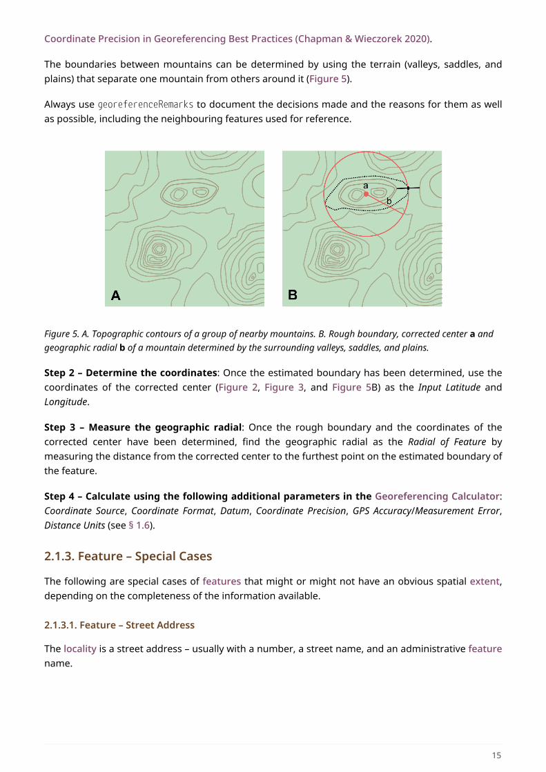
The boundaries between mountains can be determined by using the terrain (valleys, saddles, andplains) that separate one mountain from others around it (Figure 5).

Always use georeferenceRemarks to document the decisions made and the reasons for them as wellas possible, including the neighbouring features used for reference.

Figure 5. A. Topographic contours of a group of nearby mountains. B. Rough boundary, corrected center a andgeographic radial b of a mountain determined by the surrounding valleys, saddles, and plains.

Step 2 – Determine the coordinates: Once the estimated boundary has been determined, use thecoordinates of the corrected center (Figure 2, Figure 3, and Figure 5B) as the Input Latitude andLongitude.

Step 3 – Measure the geographic radial: Once the rough boundary and the coordinates of thecorrected center have been determined, find the geographic radial as the Radial of Feature bymeasuring the distance from the corrected center to the furthest point on the estimated boundary ofthe feature.

Step 4 – Calculate using the following additional parameters in the Georeferencing Calculator:Coordinate Source, Coordinate Format, Datum, Coordinate Precision, GPS Accuracy/Measurement Error,Distance Units (see § 1.6).

2.1.3. Feature – Special Cases

The following are special cases of features that might or might not have an obvious spatial extent,depending on the completeness of the information available.

2.1.3.1. Feature – Street Address

The locality is a street address – usually with a number, a street name, and an administrative featurename.

15

Examples

• "Av. Angel Gallardo 470, Buenos Aires, Argentina"

• "1 Orchard Lane, Berkeley, CA"

• "21054 Baldersleigh Road, Guyra, NSW" (indicates that the locality is 21.054 km from thebeginning of Baldersleigh Road).

Locality Type: Geographic feature only

Step 1 – Determine the feature boundaries: Locate the address using a site such as Google Maps,Mapquest or OpenStreetMap.

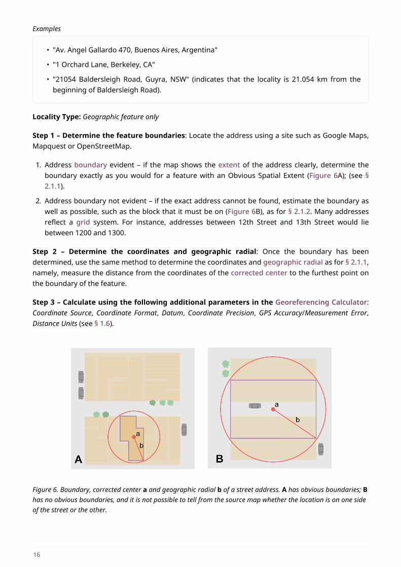
1. Address boundary evident – if the map shows the extent of the address clearly, determine theboundary exactly as you would for a feature with an Obvious Spatial Extent (Figure 6A); (see §2.1.1).

2. Address boundary not evident – if the exact address cannot be found, estimate the boundary aswell as possible, such as the block that it must be on (Figure 6B), as for § 2.1.2. Many addressesreflect a grid system. For instance, addresses between 12th Street and 13th Street would liebetween 1200 and 1300.

Step 2 – Determine the coordinates and geographic radial: Once the boundary has beendetermined, use the same method to determine the coordinates and geographic radial as for § 2.1.1,namely, measure the distance from the coordinates of the corrected center to the furthest point onthe boundary of the feature.

Step 3 – Calculate using the following additional parameters in the Georeferencing Calculator:Coordinate Source, Coordinate Format, Datum, Coordinate Precision, GPS Accuracy/Measurement Error,Distance Units (see § 1.6).

Figure 6. Boundary, corrected center a and geographic radial b of a street address. A has obvious boundaries; Bhas no obvious boundaries, and it is not possible to tell from the source map whether the location is on one sideof the street or the other.

16

2.1.3.2. Feature – Property

The locality is a property – a ranch, rancho, station, farm, finca, grange, granja, estância, plantation,hacienda, fazenda, manor, holding, estate, spread, acreage, orchard, steading, parcel, terreno, etc.

Examples

• "Victoria River Station"

• "Mathae Ranch"

• "Estancia 9 de Julio"

Locality Type: Geographic feature only

Step 1 – Determine the feature boundaries: Locate the property using whatever sources you can.You may have to resort to a cadastral map.

1. Property boundary evident – if the map shows the extent of the property, determine theboundary exactly as you would for § 2.1.1).

2. Property boundary not evident – if the full extent of the property cannot be found, it should stillbe possible to determine some part of it confidently, and the rest with less certainty. Delimit theouter, uncertain feature boundaries as usual by following § 2.1.2. In addition, determine theboundaries of the part of the property that is obvious following § 2.1.1.

Step 2 – Determine the coordinates and geographic radial:

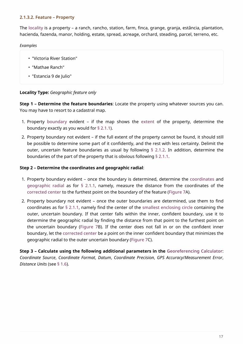
1. Property boundary evident – once the boundary is determined, determine the coordinates andgeographic radial as for § 2.1.1, namely, measure the distance from the coordinates of thecorrected center to the furthest point on the boundary of the feature (Figure 7A).

2. Property boundary not evident – once the outer boundaries are determined, use them to findcoordinates as for § 2.1.1, namely find the center of the smallest enclosing circle containing theouter, uncertain boundary. If that center falls within the inner, confident boundary, use it todetermine the geographic radial by finding the distance from that point to the furthest point onthe uncertain boundary (Figure 7B). If the center does not fall in or on the confident innerboundary, let the corrected center be a point on the inner confident boundary that minimizes thegeographic radial to the outer uncertain boundary (Figure 7C).

Step 3 – Calculate using the following additional parameters in the Georeferencing Calculator:Coordinate Source, Coordinate Format, Datum, Coordinate Precision, GPS Accuracy/Measurement Error,Distance Units (see § 1.6).

17

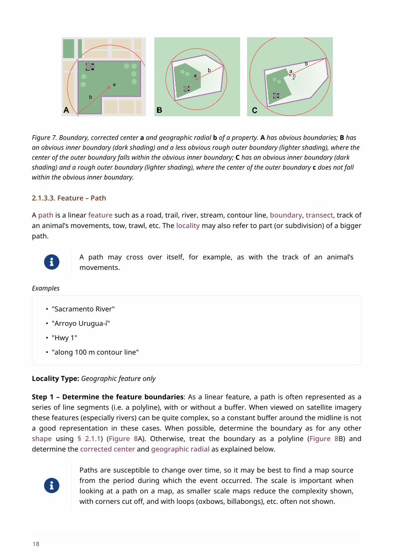
Figure 7. Boundary, corrected center a and geographic radial b of a property. A has obvious boundaries; B hasan obvious inner boundary (dark shading) and a less obvious rough outer boundary (lighter shading), where thecenter of the outer boundary falls within the obvious inner boundary; C has an obvious inner boundary (darkshading) and a rough outer boundary (lighter shading), where the center of the outer boundary c does not fallwithin the obvious inner boundary.

2.1.3.3. Feature – Path

A path is a linear feature such as a road, trail, river, stream, contour line, boundary, transect, track ofan animal’s movements, tow, trawl, etc. The locality may also refer to part (or subdivision) of a biggerpath.

A path may cross over itself, for example, as with the track of an animal’smovements.

Examples

• "Sacramento River"

• "Arroyo Urugua-í"

• "Hwy 1"

• "along 100 m contour line"

Locality Type: Geographic feature only

Step 1 – Determine the feature boundaries: As a linear feature, a path is often represented as aseries of line segments (i.e. a polyline), with or without a buffer. When viewed on satellite imagerythese features (especially rivers) can be quite complex, so a constant buffer around the midline is nota good representation in these cases. When possible, determine the boundary as for any othershape using § 2.1.1) (Figure 8A). Otherwise, treat the boundary as a polyline (Figure 8B) anddetermine the corrected center and geographic radial as explained below.

Paths are susceptible to change over time, so it may be best to find a map sourcefrom the period during which the event occurred. The scale is important whenlooking at a path on a map, as smaller scale maps reduce the complexity shown,with corners cut off, and with loops (oxbows, billabongs), etc. often not shown.

18

Contour Lines — these are linear features defined by elevation or depth. The horizontal width of thebuffer around the contour line depends on the uncertainty in elevation or depth due to acombination of the stated range and the imprecision with which the value was recorded.

If a single value is given for an elevation (or depth knowing that the location was at the bottom of awaterbody), treat the path as a linear feature with a buffer around it, where the buffer is a verticaldistance from the contour, not a horizontal one. The size of the vertical buffer should be equal to theprecision with which the elevation is recorded. For example, if the precision is 100 feet (e.g. theprecision of an elevation recorded as "2600 ft"), then the buffer is 100 vertical feet. Determine theshape of the feature using lines interpolated (or measured) one half of the buffer distance below thegiven contour and one half the buffer distance above the given contour (e.g. at 2550 feet and 2650feet for the elevation example "2600 ft").

If an elevational range is given (e.g. 100-200 m), it is difficult to know whether the range wasintended to encompass uncertainties in elevation or just the elevational bounds for the Location. Tobe conservative, we have to assume that it does not account for uncertainty in elevation and we needto add a buffer as described above around the upper and lower limits of the given range. For theexample "100 - 200 m" the buffer is 100 m, so the lower boundary of the shape would be at 100 - 50 =50 m and the upper boundary would be defined by 200 + 50 = 250 m.

Buffers might require interpolation on a topographic map if they do not correspondwith the printed contour lines (Figure 8C).

These considerations can apply equally to bathymetry where contours are available, bearing in mindthat some bathymetric contours are quite coarse and that most depths given in locality descriptionsare actually above the bottom of the waterbody.

Step 2 – Determine the coordinates and geographic radial: If the boundary can be determined,treat as for § 2.1.1, namely, measure the distance from the coordinates of the corrected center tothe furthest point on the boundary of the feature (Figure 8A).

If the feature must be treated as a polyline, draw a straight line connecting the ends of the polylineand determine its midpoint. If the midpoint falls on the polyline, that will be the center (no need forcorrection), and the geographic radial will be the distance from that point to either of the endpointsof the polyline. If the midpoint does not fall on the polyline, move it to the point on the polyline thatminimizes the distance to both endpoints. This is the corrected center and the distance to theendpoints is the geographic radial (Figure 8B).

Step 3 – Calculate using the following additional parameters in the Georeferencing Calculator:Coordinate Source, Coordinate Format, Datum, Coordinate Precision, GPS Accuracy/Measurement Error,Distance Units (see § 1.6).

19

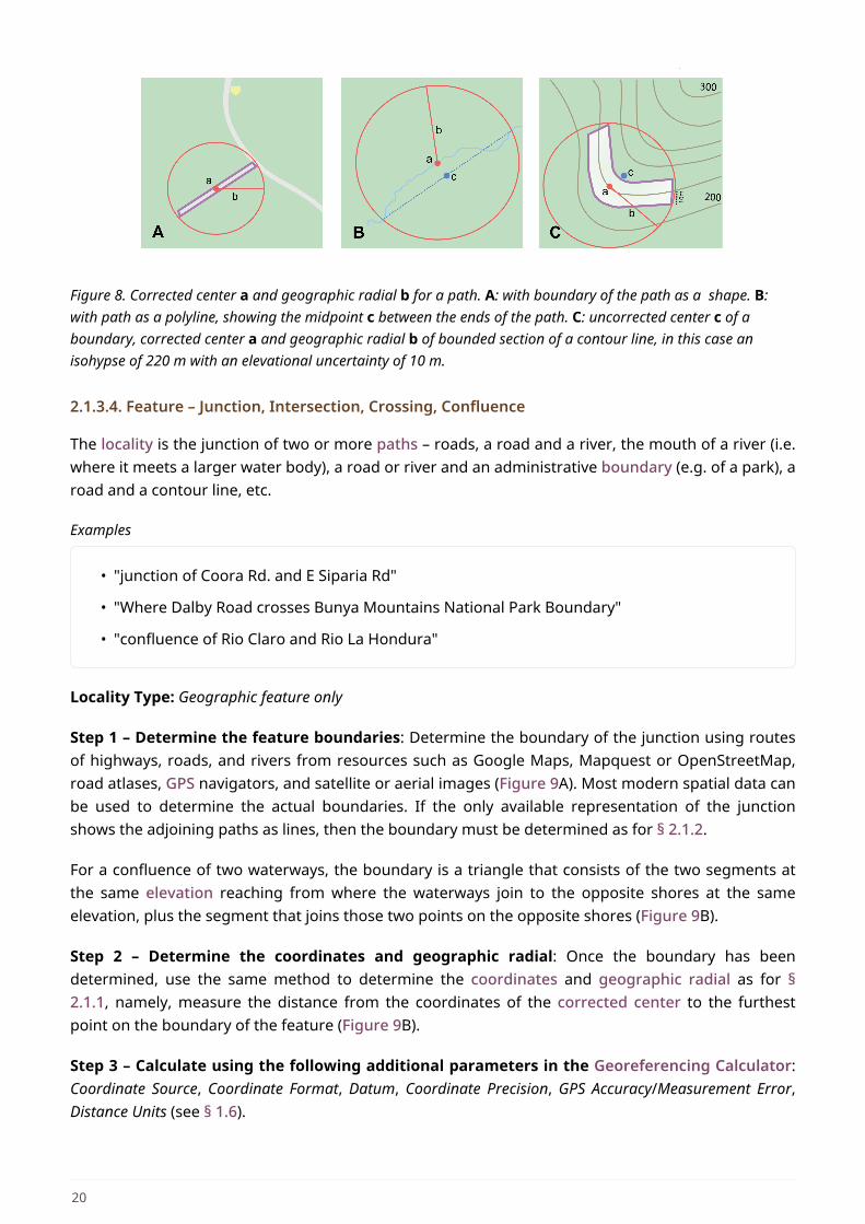
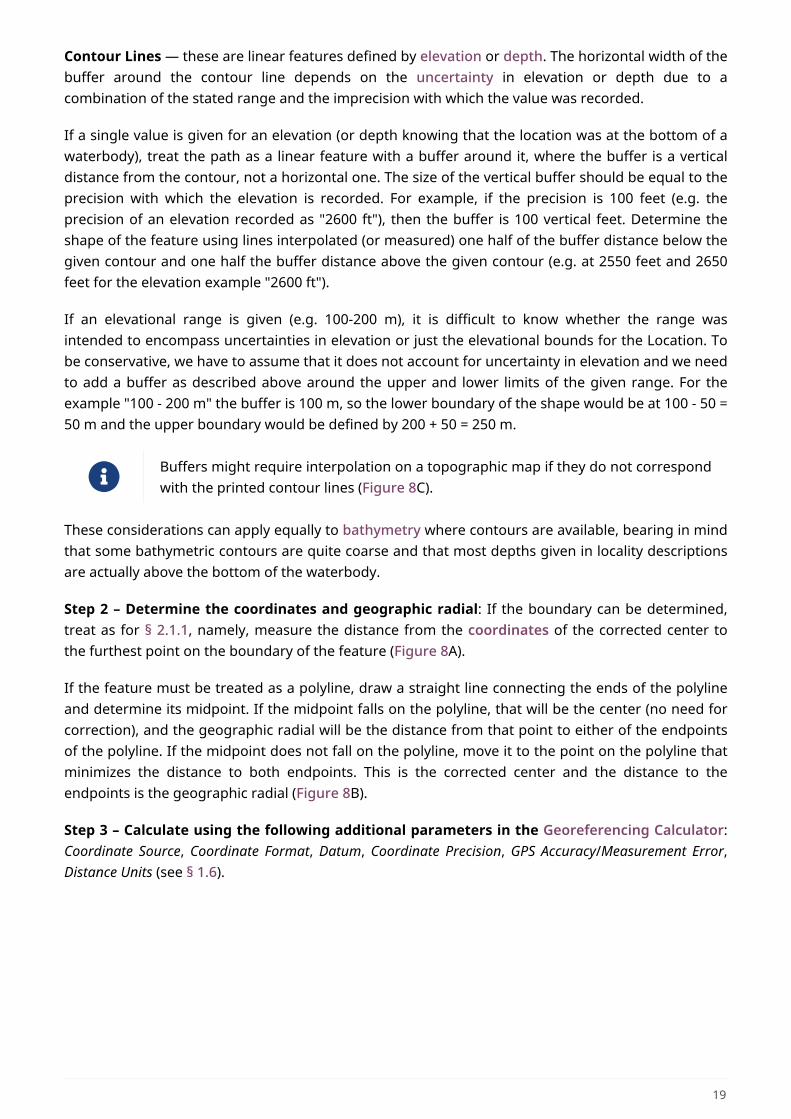
Figure 8. Corrected center a and geographic radial b for a path. A: with boundary of the path as a shape. B:with path as a polyline, showing the midpoint c between the ends of the path. C: uncorrected center c of aboundary, corrected center a and geographic radial b of bounded section of a contour line, in this case anisohypse of 220 m with an elevational uncertainty of 10 m.

2.1.3.4. Feature – Junction, Intersection, Crossing, Confluence

The locality is the junction of two or more paths – roads, a road and a river, the mouth of a river (i.e.where it meets a larger water body), a road or river and an administrative boundary (e.g. of a park), aroad and a contour line, etc.

Examples

• "junction of Coora Rd. and E Siparia Rd"

• "Where Dalby Road crosses Bunya Mountains National Park Boundary"

• "confluence of Rio Claro and Rio La Hondura"

Locality Type: Geographic feature only

Step 1 – Determine the feature boundaries: Determine the boundary of the junction using routesof highways, roads, and rivers from resources such as Google Maps, Mapquest or OpenStreetMap,road atlases, GPS navigators, and satellite or aerial images (Figure 9A). Most modern spatial data canbe used to determine the actual boundaries. If the only available representation of the junctionshows the adjoining paths as lines, then the boundary must be determined as for § 2.1.2.

For a confluence of two waterways, the boundary is a triangle that consists of the two segments atthe same elevation reaching from where the waterways join to the opposite shores at the sameelevation, plus the segment that joins those two points on the opposite shores (Figure 9B).

Step 2 – Determine the coordinates and geographic radial: Once the boundary has beendetermined, use the same method to determine the coordinates and geographic radial as for §2.1.1, namely, measure the distance from the coordinates of the corrected center to the furthestpoint on the boundary of the feature (Figure 9B).

Step 3 – Calculate using the following additional parameters in the Georeferencing Calculator:Coordinate Source, Coordinate Format, Datum, Coordinate Precision, GPS Accuracy/Measurement Error,Distance Units (see § 1.6).

20

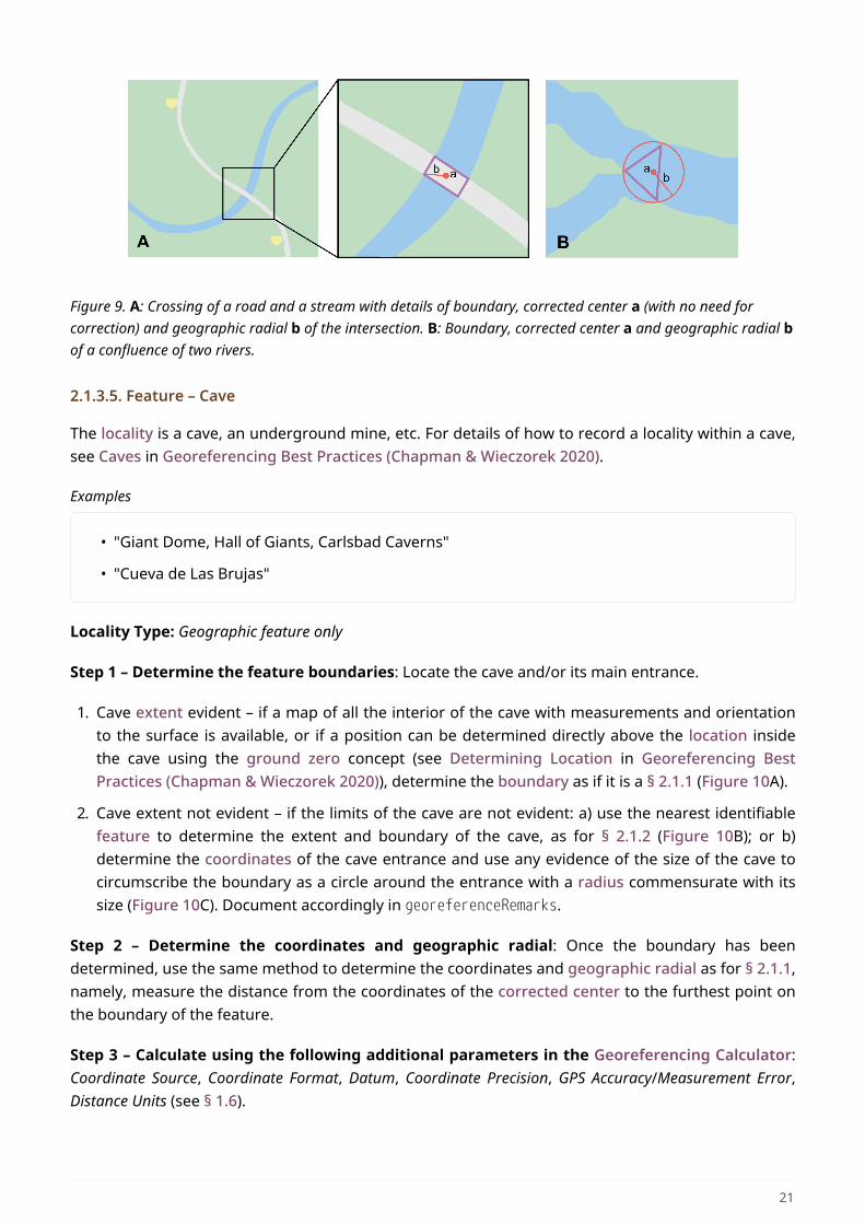
Figure 9. A: Crossing of a road and a stream with details of boundary, corrected center a (with no need forcorrection) and geographic radial b of the intersection. B: Boundary, corrected center a and geographic radial bof a confluence of two rivers.

2.1.3.5. Feature – Cave

The locality is a cave, an underground mine, etc. For details of how to record a locality within a cave,see Caves in Georeferencing Best Practices (Chapman & Wieczorek 2020).

Examples

• "Giant Dome, Hall of Giants, Carlsbad Caverns"

• "Cueva de Las Brujas"

Locality Type: Geographic feature only

Step 1 – Determine the feature boundaries: Locate the cave and/or its main entrance.

1. Cave extent evident – if a map of all the interior of the cave with measurements and orientationto the surface is available, or if a position can be determined directly above the location insidethe cave using the ground zero concept (see Determining Location in Georeferencing BestPractices (Chapman & Wieczorek 2020)), determine the boundary as if it is a § 2.1.1 (Figure 10A).

2. Cave extent not evident – if the limits of the cave are not evident: a) use the nearest identifiablefeature to determine the extent and boundary of the cave, as for § 2.1.2 (Figure 10B); or b)determine the coordinates of the cave entrance and use any evidence of the size of the cave tocircumscribe the boundary as a circle around the entrance with a radius commensurate with itssize (Figure 10C). Document accordingly in georeferenceRemarks.

Step 2 – Determine the coordinates and geographic radial: Once the boundary has beendetermined, use the same method to determine the coordinates and geographic radial as for § 2.1.1,namely, measure the distance from the coordinates of the corrected center to the furthest point onthe boundary of the feature.

Step 3 – Calculate using the following additional parameters in the Georeferencing Calculator:Coordinate Source, Coordinate Format, Datum, Coordinate Precision, GPS Accuracy/Measurement Error,Distance Units (see § 1.6).

21

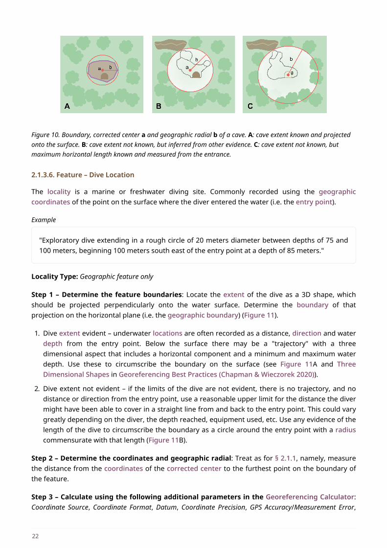
Figure 10. Boundary, corrected center a and geographic radial b of a cave. A: cave extent known and projectedonto the surface. B: cave extent not known, but inferred from other evidence. C: cave extent not known, butmaximum horizontal length known and measured from the entrance.

2.1.3.6. Feature – Dive Location

The locality is a marine or freshwater diving site. Commonly recorded using the geographiccoordinates of the point on the surface where the diver entered the water (i.e. the entry point).

Example

"Exploratory dive extending in a rough circle of 20 meters diameter between depths of 75 and100 meters, beginning 100 meters south east of the entry point at a depth of 85 meters."

Locality Type: Geographic feature only

Step 1 – Determine the feature boundaries: Locate the extent of the dive as a 3D shape, whichshould be projected perpendicularly onto the water surface. Determine the boundary of thatprojection on the horizontal plane (i.e. the geographic boundary) (Figure 11).

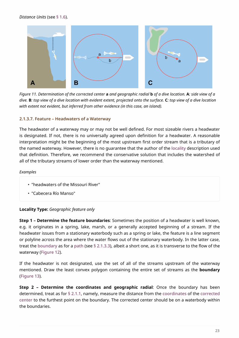
1. Dive extent evident – underwater locations are often recorded as a distance, direction and waterdepth from the entry point. Below the surface there may be a "trajectory" with a threedimensional aspect that includes a horizontal component and a minimum and maximum waterdepth. Use these to circumscribe the boundary on the surface (see Figure 11A and ThreeDimensional Shapes in Georeferencing Best Practices (Chapman & Wieczorek 2020)).

2. Dive extent not evident – if the limits of the dive are not evident, there is no trajectory, and nodistance or direction from the entry point, use a reasonable upper limit for the distance the divermight have been able to cover in a straight line from and back to the entry point. This could varygreatly depending on the diver, the depth reached, equipment used, etc. Use any evidence of thelength of the dive to circumscribe the boundary as a circle around the entry point with a radiuscommensurate with that length (Figure 11B).

Step 2 – Determine the coordinates and geographic radial: Treat as for § 2.1.1, namely, measurethe distance from the coordinates of the corrected center to the furthest point on the boundary ofthe feature.

Step 3 – Calculate using the following additional parameters in the Georeferencing Calculator:Coordinate Source, Coordinate Format, Datum, Coordinate Precision, GPS Accuracy/Measurement Error,

22

Distance Units (see § 1.6).

Figure 11. Determination of the corrected center a and geographic radial b of a dive location. A: side view of adive. B: top view of a dive location with evident extent, projected onto the surface. C: top view of a dive locationwith extent not evident, but inferred from other evidence (in this case, an island).

2.1.3.7. Feature – Headwaters of a Waterway

The headwater of a waterway may or may not be well defined. For most sizeable rivers a headwateris designated. If not, there is no universally agreed upon definition for a headwater. A reasonableinterpretation might be the beginning of the most upstream first order stream that is a tributary ofthe named waterway. However, there is no guarantee that the author of the locality description usedthat definition. Therefore, we recommend the conservative solution that includes the watershed ofall of the tributary streams of lower order than the waterway mentioned.

Examples

• "headwaters of the Missouri River"

• "Cabecera Río Manso"

Locality Type: Geographic feature only

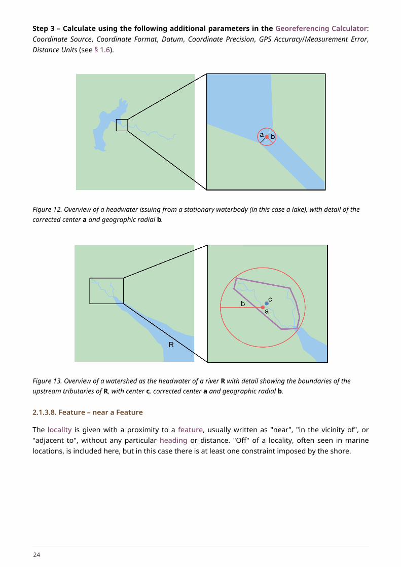
Step 1 – Determine the feature boundaries: Sometimes the position of a headwater is well known,e.g. it originates in a spring, lake, marsh, or a generally accepted beginning of a stream. If theheadwater issues from a stationary waterbody such as a spring or lake, the feature is a line segmentor polyline across the area where the water flows out of the stationary waterbody. In the latter case,treat the boundary as for a path (see § 2.1.3.3), albeit a short one, as it is transverse to the flow of thewaterway (Figure 12).

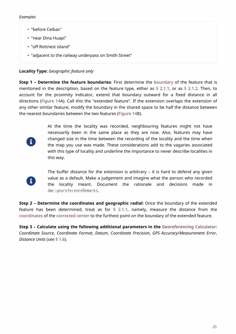
If the headwater is not designated, use the set of all of the streams upstream of the waterwaymentioned. Draw the least convex polygon containing the entire set of streams as the boundary(Figure 13).

Step 2 – Determine the coordinates and geographic radial: Once the boundary has beendetermined, treat as for § 2.1.1, namely, measure the distance from the coordinates of the correctedcenter to the furthest point on the boundary. The corrected center should be on a waterbody withinthe boundaries.

23

Step 3 – Calculate using the following additional parameters in the Georeferencing Calculator:Coordinate Source, Coordinate Format, Datum, Coordinate Precision, GPS Accuracy/Measurement Error,Distance Units (see § 1.6).

Figure 12. Overview of a headwater issuing from a stationary waterbody (in this case a lake), with detail of thecorrected center a and geographic radial b.

Figure 13. Overview of a watershed as the headwater of a river R with detail showing the boundaries of theupstream tributaries of R, with center c, corrected center a and geographic radial b.

2.1.3.8. Feature – near a Feature

The locality is given with a proximity to a feature, usually written as "near", "in the vicinity of", or"adjacent to", without any particular heading or distance. "Off" of a locality, often seen in marinelocations, is included here, but in this case there is at least one constraint imposed by the shore.

24

Examples

• "before Ceibas"

• "near Dina Huapi"

• "off Rottnest island"

• "adjacent to the railway underpass on Smith Street"

Locality Type: Geographic feature only

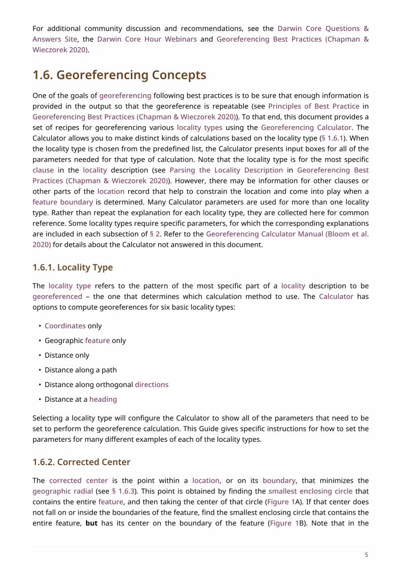
Step 1 – Determine the feature boundaries: First determine the boundary of the feature that ismentioned in the description, based on the feature type, either as § 2.1.1, or as § 2.1.2. Then, toaccount for the proximity indicator, extend that boundary outward for a fixed distance in alldirections (Figure 14A). Call this the "extended feature". If the extension overlaps the extension ofany other similar feature, modify the boundary in the shared space to be half the distance betweenthe nearest boundaries between the two features (Figure 14B).

At the time the locality was recorded, neighbouring features might not havenecessarily been in the same place as they are now. Also, features may havechanged size in the time between the recording of the locality and the time whenthe map you use was made. These considerations add to the vagaries associatedwith this type of locality and underline the importance to never describe localities inthis way.

The buffer distance for the extension is arbitrary – it is hard to defend any givenvalue as a default. Make a judgement and imagine what the person who recordedthe locality meant. Document the rationale and decisions made indwc:georeferenceRemarks.

Step 2 – Determine the coordinates and geographic radial: Once the boundary of the extendedfeature has been determined, treat as for § 2.1.1, namely, measure the distance from thecoordinates of the corrected center to the furthest point on the boundary of the extended feature.

Step 3 – Calculate using the following additional parameters in the Georeferencing Calculator:Coordinate Source, Coordinate Format, Datum, Coordinate Precision, GPS Accuracy/Measurement Error,Distance Units (see § 1.6).

25

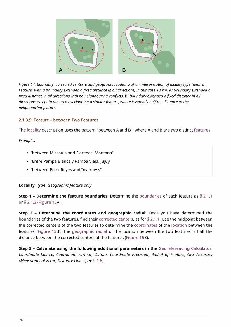
Figure 14. Boundary, corrected center a and geographic radial b of an interpretation of locality type "near aFeature" with a boundary extended a fixed distance in all directions, in this case 10 km. A: Boundary extended afixed distance in all directions with no neighbouring conflicts. B: Boundary extended a fixed distance in alldirections except in the area overlapping a similar feature, where it extends half the distance to theneighbouring feature.

2.1.3.9. Feature – between Two Features

The locality description uses the pattern "between A and B", where A and B are two distinct features.

Examples

• "between Missoula and Florence, Montana"

• "Entre Pampa Blanca y Pampa Vieja, Jujuy"

• "between Point Reyes and Inverness"

Locality Type: Geographic feature only

Step 1 – Determine the feature boundaries: Determine the boundaries of each feature as § 2.1.1or § 2.1.2 (Figure 15A).

Step 2 – Determine the coordinates and geographic radial: Once you have determined theboundaries of the two features, find their corrected centers, as for § 2.1.1. Use the midpoint betweenthe corrected centers of the two features to determine the coordinates of the location between thefeatures (Figure 15B). The geographic radial of the location between the two features is half thedistance between the corrected centers of the features (Figure 15B).

Step 3 – Calculate using the following additional parameters in the Georeferencing Calculator:Coordinate Source, Coordinate Format, Datum, Coordinate Precision, Radial of Feature, GPS Accuracy/Measurement Error, Distance Units (see § 1.6).

26

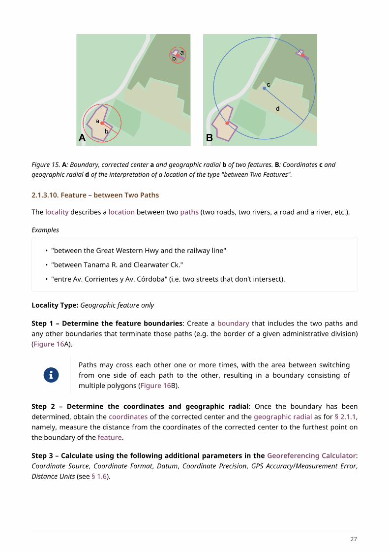
Figure 15. A: Boundary, corrected center a and geographic radial b of two features. B: Coordinates c andgeographic radial d of the interpretation of a location of the type "between Two Features".

2.1.3.10. Feature – between Two Paths

The locality describes a location between two paths (two roads, two rivers, a road and a river, etc.).

Examples

• "between the Great Western Hwy and the railway line"

• "between Tanama R. and Clearwater Ck."

• "entre Av. Corrientes y Av. Córdoba" (i.e. two streets that don’t intersect).

Locality Type: Geographic feature only

Step 1 – Determine the feature boundaries: Create a boundary that includes the two paths andany other boundaries that terminate those paths (e.g. the border of a given administrative division)(Figure 16A).

Paths may cross each other one or more times, with the area between switchingfrom one side of each path to the other, resulting in a boundary consisting ofmultiple polygons (Figure 16B).

Step 2 – Determine the coordinates and geographic radial: Once the boundary has beendetermined, obtain the coordinates of the corrected center and the geographic radial as for § 2.1.1,namely, measure the distance from the coordinates of the corrected center to the furthest point onthe boundary of the feature.

Step 3 – Calculate using the following additional parameters in the Georeferencing Calculator:Coordinate Source, Coordinate Format, Datum, Coordinate Precision, GPS Accuracy/Measurement Error,Distance Units (see § 1.6).

27

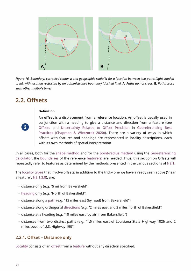
Figure 16. Boundary, corrected center a and geographic radial b for a location between two paths (light shadedarea), with location restricted by an administrative boundary (dashed line). A: Paths do not cross. B: Paths crosseach other multiple times.

2.2. Offsets

Definition

An offset is a displacement from a reference location. An offset is usually used inconjunction with a heading to give a distance and direction from a feature (seeOffsets and Uncertainty Related to Offset Precision in Georeferencing BestPractices (Chapman & Wieczorek 2020)). There are a variety of ways in whichoffsets with features and headings are represented in locality descriptions, eachwith its own methods of spatial interpretation.

In all cases, both for the shape method and for the point-radius method using the GeoreferencingCalculator, the boundaries of the reference feature(s) are needed. Thus, this section on Offsets willrepeatedly refer to features as determined by the methods presented in the various sections of § 2.1.

The locality types that involve offsets, in addition to the tricky one we have already seen above ("neara feature", § 2.1.3.8), are:

• distance only (e.g. "5 mi from Bakersfield")

• heading only (e.g. "North of Bakersfield")

• distance along a path (e.g. "13 miles east (by road) from Bakersfield")

• distance along orthogonal directions (e.g. "2 miles east and 3 miles north of Bakersfield")

• distance at a heading (e.g. "10 miles east (by air) from Bakersfield")

• distances from two distinct paths (e.g. "1.5 miles east of Louisiana State Highway 1026 and 2miles south of U.S. Highway 190")

2.2.1. Offset – Distance only

Locality consists of an offset from a feature without any direction specified.

28

Examples

• "5 km outside Calgary"

• "12 km de Purmamarca"

Locality Type: Distance only

Step 1 – Determine the feature boundaries: Determine the boundary of the feature as you wouldfor § 2.1.3.8, except that the distance to use for the buffer is the distance given in the localitydescription, and there is no need to account for the proximity of other features.

Step 2 – Determine the coordinates and geographic radial: Once the boundary has beendetermined, obtain the coordinates and the geographic radial as for § 2.1.1, namely, measure thedistance from the coordinates of the corrected center to the furthest point on the boundary of thefeature.

Offset Distance: Set to 0. The distance has already been incorporated in the determination of theboundary. Use the distance and units given in the locality description to georeference using theGeoreferencing Calculator.

Distance Precision: Though the Offset Distance is set to zero, the Distance Precision should still be set(see § 1.6.13) to account for this source of uncertainty.

Step 3 – Calculate using the following additional parameters in the Georeferencing Calculator:Coordinate source, Coordinate Format, Datum, Coordinate Precision, Measurement Error (see § 1.6).

2.2.2. Offset – Heading only

The locality consists of a direction from a feature without any distance specified. Note that seldom issuch information given alone; there is usually some supporting information. For example, the localitymay have higher-level geographic information such as "East of Albuquerque, Bernalillo County, NewMexico". This provides a stopping point (the county border), and should allow you to georeferencethe locality. Alternatively, there might be another similar feature in the direction of the givenheading that can constrain the offset.

Examples

• "N Palmetto"

• "W of Berkeley"

• "Saladillo E"

• "Al N de Saladillo"

Locality Type: Geographic feature only

Step 1 – Determine the feature boundaries: First determine the boundary of the given featurebased on the feature type, either as for § 2.1.1, or as for § 2.1.2. Then, to account for the offset at aheading, extend that boundary outward in a cone defined by the heading uncertainty (see Offset –

29

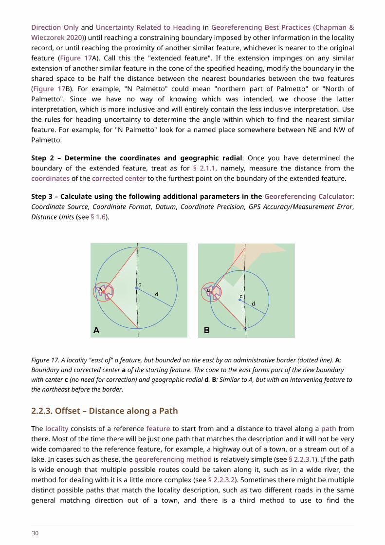
Direction Only and Uncertainty Related to Heading in Georeferencing Best Practices (Chapman &Wieczorek 2020)) until reaching a constraining boundary imposed by other information in the localityrecord, or until reaching the proximity of another similar feature, whichever is nearer to the originalfeature (Figure 17A). Call this the "extended feature". If the extension impinges on any similarextension of another similar feature in the cone of the specified heading, modify the boundary in theshared space to be half the distance between the nearest boundaries between the two features(Figure 17B). For example, "N Palmetto" could mean "northern part of Palmetto" or "North ofPalmetto". Since we have no way of knowing which was intended, we choose the latterinterpretation, which is more inclusive and will entirely contain the less inclusive interpretation. Usethe rules for heading uncertainty to determine the angle within which to find the nearest similarfeature. For example, for "N Palmetto" look for a named place somewhere between NE and NW ofPalmetto.

Step 2 – Determine the coordinates and geographic radial: Once you have determined theboundary of the extended feature, treat as for § 2.1.1, namely, measure the distance from thecoordinates of the corrected center to the furthest point on the boundary of the extended feature.

Step 3 – Calculate using the following additional parameters in the Georeferencing Calculator:Coordinate Source, Coordinate Format, Datum, Coordinate Precision, GPS Accuracy/Measurement Error,Distance Units (see § 1.6).

Figure 17. A locality "east of" a feature, but bounded on the east by an administrative border (dotted line). A:Boundary and corrected center a of the starting feature. The cone to the east forms part of the new boundarywith center c (no need for correction) and geographic radial d. B: Similar to A, but with an intervening feature tothe northeast before the border.

2.2.3. Offset – Distance along a Path

The locality consists of a reference feature to start from and a distance to travel along a path fromthere. Most of the time there will be just one path that matches the description and it will not be verywide compared to the reference feature, for example, a highway out of a town, or a stream out of alake. In cases such as these, the georeferencing method is relatively simple (see § 2.2.3.1). If the pathis wide enough that multiple possible routes could be taken along it, such as in a wide river, themethod for dealing with it is a little more complex (see § 2.2.3.2). Sometimes there might be multipledistinct possible paths that match the locality description, such as two different roads in the samegeneral matching direction out of a town, and there is a third method to use to find the

30

georeference (see § 2.2.3.3). In all cases, the georeference will cover a segment of the path orpossible paths that includes all the sources of uncertainty. Though there might be a headingmentioned in the locality description (e.g. "9 km S El Bolsón on Ruta 40"), it serves only to constrainwhich path or paths are possible, and does not contribute uncertainty due to heading precision.

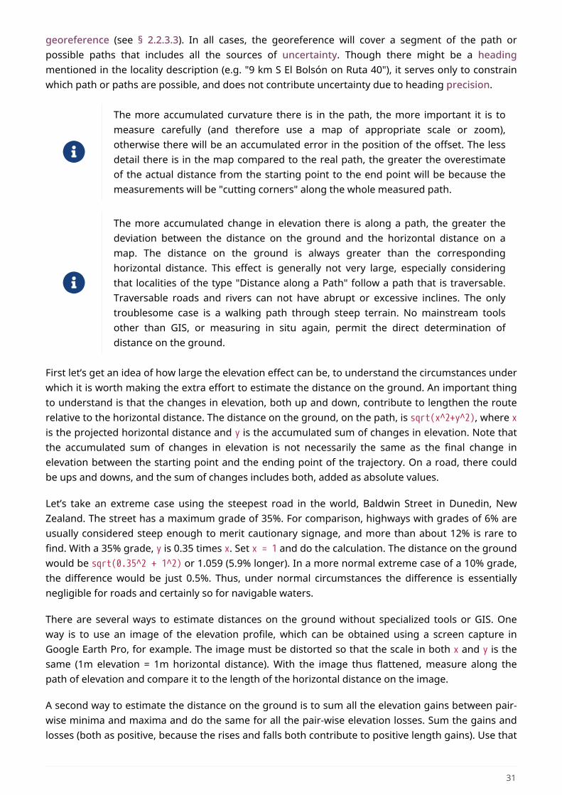
The more accumulated curvature there is in the path, the more important it is tomeasure carefully (and therefore use a map of appropriate scale or zoom),otherwise there will be an accumulated error in the position of the offset. The lessdetail there is in the map compared to the real path, the greater the overestimateof the actual distance from the starting point to the end point will be because themeasurements will be "cutting corners" along the whole measured path.

The more accumulated change in elevation there is along a path, the greater thedeviation between the distance on the ground and the horizontal distance on amap. The distance on the ground is always greater than the correspondinghorizontal distance. This effect is generally not very large, especially consideringthat localities of the type "Distance along a Path" follow a path that is traversable.Traversable roads and rivers can not have abrupt or excessive inclines. The onlytroublesome case is a walking path through steep terrain. No mainstream toolsother than GIS, or measuring in situ again, permit the direct determination ofdistance on the ground.

First let’s get an idea of how large the elevation effect can be, to understand the circumstances underwhich it is worth making the extra effort to estimate the distance on the ground. An important thingto understand is that the changes in elevation, both up and down, contribute to lengthen the routerelative to the horizontal distance. The distance on the ground, on the path, is sqrt(x^2+y^2), where xis the projected horizontal distance and y is the accumulated sum of changes in elevation. Note thatthe accumulated sum of changes in elevation is not necessarily the same as the final change inelevation between the starting point and the ending point of the trajectory. On a road, there couldbe ups and downs, and the sum of changes includes both, added as absolute values.

Let’s take an extreme case using the steepest road in the world, Baldwin Street in Dunedin, NewZealand. The street has a maximum grade of 35%. For comparison, highways with grades of 6% areusually considered steep enough to merit cautionary signage, and more than about 12% is rare tofind. With a 35% grade, y is 0.35 times x. Set x = 1 and do the calculation. The distance on the groundwould be sqrt(0.35^2 + 1^2) or 1.059 (5.9% longer). In a more normal extreme case of a 10% grade,the difference would be just 0.5%. Thus, under normal circumstances the difference is essentiallynegligible for roads and certainly so for navigable waters.

There are several ways to estimate distances on the ground without specialized tools or GIS. Oneway is to use an image of the elevation profile, which can be obtained using a screen capture inGoogle Earth Pro, for example. The image must be distorted so that the scale in both x and y is thesame (1m elevation = 1m horizontal distance). With the image thus flattened, measure along thepath of elevation and compare it to the length of the horizontal distance on the image.

A second way to estimate the distance on the ground is to sum all the elevation gains between pair-wise minima and maxima and do the same for all the pair-wise elevation losses. Sum the gains andlosses (both as positive, because the rises and falls both contribute to positive length gains). Use that

31

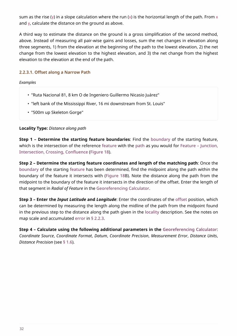
sum as the rise (y) in a slope calculation where the run (x) is the horizontal length of the path. From xand y, calculate the distance on the ground as above.

A third way to estimate the distance on the ground is a gross simplification of the second method,above. Instead of measuring all pair-wise gains and losses, sum the net changes in elevation alongthree segments, 1) from the elevation at the beginning of the path to the lowest elevation, 2) the netchange from the lowest elevation to the highest elevation, and 3) the net change from the highestelevation to the elevation at the end of the path.

2.2.3.1. Offset along a Narrow Path

Examples

• "Ruta Nacional 81, 8 km O de Ingeniero Guillermo Nicasio Juárez"

• "left bank of the Mississippi River, 16 mi downstream from St. Louis"

• "500m up Skeleton Gorge"

Locality Type: Distance along path

Step 1 – Determine the starting feature boundaries: Find the boundary of the starting feature,which is the intersection of the reference feature with the path as you would for Feature – Junction,Intersection, Crossing, Confluence (Figure 18).

Step 2 – Determine the starting feature coordinates and length of the matching path: Once theboundary of the starting feature has been determined, find the midpoint along the path within theboundary of the feature it intersects with (Figure 18B). Note the distance along the path from themidpoint to the boundary of the feature it intersects in the direction of the offset. Enter the length ofthat segment in Radial of Feature in the Georeferencing Calculator.

Step 3 – Enter the Input Latitude and Longitude: Enter the coordinates of the offset position, whichcan be determined by measuring the length along the midline of the path from the midpoint foundin the previous step to the distance along the path given in the locality description. See the notes onmap scale and accumulated error in § 2.2.3.

Step 4 – Calculate using the following additional parameters in the Georeferencing Calculator:Coordinate Source, Coordinate Format, Datum, Coordinate Precision, Measurement Error, Distance Units,Distance Precision (see § 1.6).

32

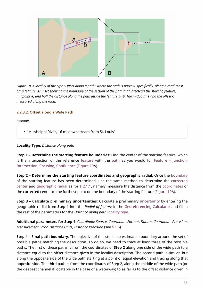
Figure 18. A locality of the type "Offset along a path" where the path is narrow, specifically, along a road "eastof" a feature. A: Inset showing the boundary of the section of the path that intersects the starting feature,midpoint a, and half the distance along the path inside the feature b. B: The midpoint a and the offset cmeasured along the road.

2.2.3.2. Offset along a Wide Path

Example

• "Mississippi River, 16 mi downstream from St. Louis"

Locality Type: Distance along path

Step 1 – Determine the starting feature boundaries: Find the center of the starting feature, whichis the intersection of the reference feature with the path as you would for Feature – Junction,Intersection, Crossing, Confluence (Figure 19A).

Step 2 – Determine the starting feature coordinates and geographic radial: Once the boundaryof the starting feature has been determined, use the same method to determine the correctedcenter and geographic radial as for § 2.1.1, namely, measure the distance from the coordinates ofthe corrected center to the furthest point on the boundary of the starting feature (Figure 19A).

Step 3 – Calculate preliminary uncertainties: Calculate a preliminary uncertainty by entering thegeographic radial from Step 1 into the Radial of feature in the Georeferencing Calculator and fill inthe rest of the parameters for the Distance along path locality type.

Additional parameters for Step 4: Coordinate Source, Coordinate Format, Datum, Coordinate Precision,Measurement Error, Distance Units, Distance Precision (see § 1.6).

Step 4 – Final path boundary: The objective of this step is to estimate a boundary around the set ofpossible paths matching the description. To do so, we need to trace at least three of the possiblepaths. The first of these paths is from the coordinates of Step 2 along one side of the wide path to adistance equal to the offset distance given in the locality description. The second path is similar, butalong the opposite side of the wide path starting at a point of equal elevation and tracing along thatopposite side. The third path is from the coordinates of Step 2, along the middle of the wide path (orthe deepest channel if locatable in the case of a waterway) to as far as to the offset distance given in

33

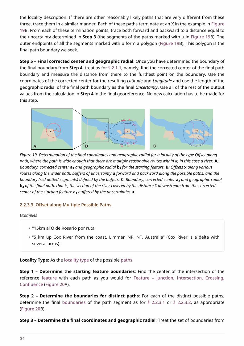
the locality description. If there are other reasonably likely paths that are very different from thesethree, trace them in a similar manner. Each of these paths terminate at an X in the example in Figure19B. From each of these termination points, trace both forward and backward to a distance equal tothe uncertainty determined in Step 3 (the segments of the paths marked with u in Figure 19B). Theouter endpoints of all the segments marked with u form a polygon (Figure 19B). This polygon is thefinal path boundary we seek.

Step 5 – Final corrected center and geographic radial: Once you have determined the boundary ofthe final boundary from Step 4, treat as for § 2.1.1, namely, find the corrected center of the final pathboundary and measure the distance from there to the furthest point on the boundary. Use thecoordinates of the corrected center for the resulting Latitude and Longitude and use the length of thegeographic radial of the final path boundary as the final Uncertainty. Use all of the rest of the outputvalues from the calculation in Step 4 in the final georeference. No new calculation has to be made forthis step.

Figure 19. Determination of the final coordinates and geographic radial for a locality of the type Offset alongpath, where the path is wide enough that there are multiple reasonable routes within it, in this case a river. A:Boundary, corrected center a₁ and geographic radial b₁ for the starting feature. B: Offsets x along variousroutes along the wider path, buffers of uncertainty u forward and backward along the possible paths, and theboundary (red dotted segments) defined by the buffers. C: Boundary, corrected center a₂ and geographic radialb₂ of the final path, that is, the section of the river covered by the distance X downstream from the correctedcenter of the starting feature a₁ buffered by the uncertainties u.

2.2.3.3. Offset along Multiple Possible Paths

Examples

• "15km al O de Rosario por ruta"

• “5 km up Cox River from the coast, Limmen NP, NT, Australia” (Cox River is a delta withseveral arms).

Locality Type: As the locality type of the possible paths.

Step 1 – Determine the starting feature boundaries: Find the center of the intersection of thereference feature with each path as you would for Feature – Junction, Intersection, Crossing,Confluence (Figure 20A).

Step 2 – Determine the boundaries for distinct paths: For each of the distinct possible paths,determine the final boundaries of the path segment as for § 2.2.3.1 or § 2.2.3.2, as appropriate(Figure 20B).

Step 3 – Determine the final coordinates and geographic radial: Treat the set of boundaries from

34

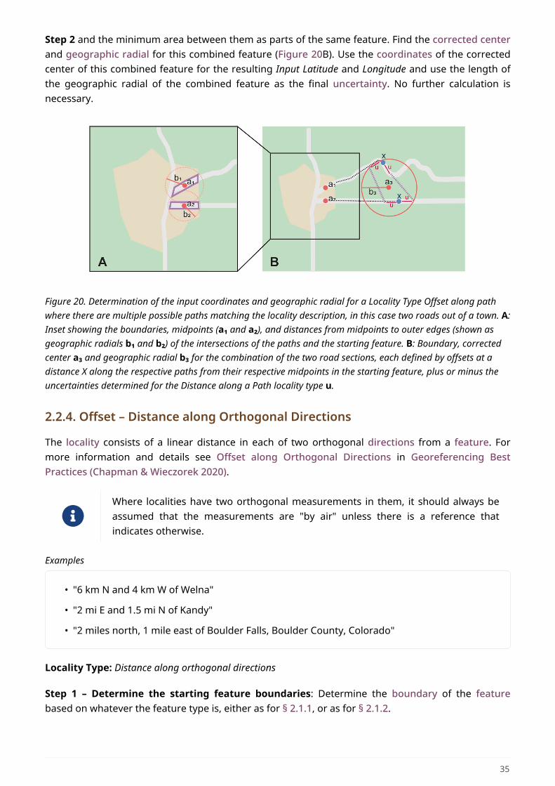
Step 2 and the minimum area between them as parts of the same feature. Find the corrected centerand geographic radial for this combined feature (Figure 20B). Use the coordinates of the correctedcenter of this combined feature for the resulting Input Latitude and Longitude and use the length ofthe geographic radial of the combined feature as the final uncertainty. No further calculation isnecessary.

Figure 20. Determination of the input coordinates and geographic radial for a Locality Type Offset along pathwhere there are multiple possible paths matching the locality description, in this case two roads out of a town. A:Inset showing the boundaries, midpoints (a₁ and a₂), and distances from midpoints to outer edges (shown asgeographic radials b₁ and b₂) of the intersections of the paths and the starting feature. B: Boundary, correctedcenter a₃ and geographic radial b₃ for the combination of the two road sections, each defined by offsets at adistance X along the respective paths from their respective midpoints in the starting feature, plus or minus theuncertainties determined for the Distance along a Path locality type u.

2.2.4. Offset – Distance along Orthogonal Directions

The locality consists of a linear distance in each of two orthogonal directions from a feature. Formore information and details see Offset along Orthogonal Directions in Georeferencing BestPractices (Chapman & Wieczorek 2020).

Where localities have two orthogonal measurements in them, it should always beassumed that the measurements are "by air" unless there is a reference thatindicates otherwise.

Examples

• "6 km N and 4 km W of Welna"

• "2 mi E and 1.5 mi N of Kandy"

• "2 miles north, 1 mile east of Boulder Falls, Boulder County, Colorado"

Locality Type: Distance along orthogonal directions

Step 1 – Determine the starting feature boundaries: Determine the boundary of the featurebased on whatever the feature type is, either as for § 2.1.1, or as for § 2.1.2.

35

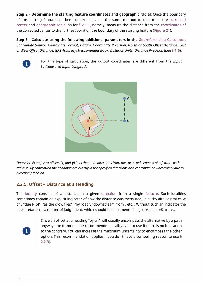
Step 2 – Determine the starting feature coordinates and geographic radial: Once the boundaryof the starting feature has been determined, use the same method to determine the correctedcenter and geographic radial as for § 2.1.1, namely, measure the distance from the coordinates ofthe corrected center to the furthest point on the boundary of the starting feature (Figure 21).

Step 3 – Calculate using the following additional parameters in the Georeferencing Calculator:Coordinate Source, Coordinate Format, Datum, Coordinate Precision, North or South Offset Distance, Eastor West Offset Distance, GPS Accuracy/Measurement Error, Distance Units, Distance Precision (see § 1.6).

For this type of calculation, the output coordinates are different from the InputLatitude and Input Longitude.

Figure 21. Example of offsets (x, and y) in orthogonal directions from the corrected center a of a feature withradial b. By convention the headings are exactly in the specified directions and contribute no uncertainty due todirection precision.

2.2.5. Offset – Distance at a Heading

The locality consists of a distance in a given direction from a single feature. Such localitiessometimes contain an explicit indicator of how the distance was measured, (e.g. "by air", "air miles Wof", "due N of", "as the crow flies", "by road", "downstream from", etc.). Without such an indicator theinterpretation is a matter of judgement, which should be documented in georeferenceRemarks.

Since an offset at a heading "by air" will usually encompass the alternative by a pathanyway, the former is the recommended locality type to use if there is no indicationto the contrary. You can increase the maximum uncertainty to encompass the otheroption. This recommendation applies if you don’t have a compelling reason to use §2.2.3).

36

The addition of an adverbial modifier to the distance part of a locality description(e.g. "about 25 km WNW Campinas"), while an honest observation, should not affectthe determination of the geographic coordinates or the overall uncertainty.

Examples

• "50 miles W of Las Vegas"

• "10.2 km E de Amamá"

• "16 mi downstream from St Louis on the Mississippi River"

• "about 25 km WNW of Campinas"

• "10 mi E (by air) Yerevan"

Locality Type: Distance at a heading

Step 1 – Determine the starting feature boundaries: Determine the boundary of the featurebased on whatever the feature type is, either as for § 2.1.1, or as for § 2.1.2.

Step 2 – Determine the starting feature coordinates and geographic radial: Once the boundaryhas been determined, obtain the coordinates and the geographic radial as for § 2.1.1, namely,measure the distance from the coordinates of the corrected center to the furthest point on theboundary of the feature.

Step 3 – Calculate using the following additional parameters in the Georeferencing Calculator:Coordinate Source, Coordinate Format, Datum, Coordinate Precision, Direction, Offset Distance, GPSAccuracy/Measurement Error, Distance Units, Distance Precision (see § 1.6).

For this type of calculation, the output coordinates are different from the InputLatitude and Input Longitude.

2.2.6. Offset – Distances from Two Distinct Paths

The locality consists of orthogonal offset distances, one from each of two distinct paths.

Example

• "1.5 mi E LA Hwy. 1026 and 2 mi S U.S. 190"

Locality Type: Distance along path

Although this is not technically a distance along a path, the choice of this locality type in theGeoreferencing Calculator will allow all of the relevant parameters to be entered.

Step 1 – Determine the feature boundaries: Determine the boundaries of the area matching thelocality description by "transporting" each path by its given offset distance and direction. Thetransported paths will then overlap, each one having its corresponding buffer due to distanceprecision and path widths around it. This overlap of the two buffered areas defines the extent of the

37

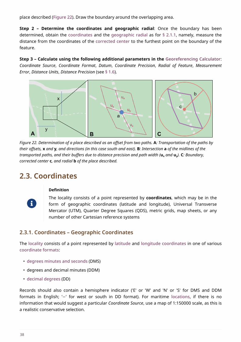
place described (Figure 22). Draw the boundary around the overlapping area.

Step 2 – Determine the coordinates and geographic radial: Once the boundary has beendetermined, obtain the coordinates and the geographic radial as for § 2.1.1, namely, measure thedistance from the coordinates of the corrected center to the furthest point on the boundary of thefeature.

Step 3 – Calculate using the following additional parameters in the Georeferencing Calculator:Coordinate Source, Coordinate Format, Datum, Coordinate Precision, Radial of Feature, MeasurementError, Distance Units, Distance Precision (see § 1.6).

Figure 22. Determination of a place described as an offset from two paths. A: Transportation of the paths bytheir offsets, x and y, and directions (in this case south and east). B: Intersection a of the midlines of thetransported paths, and their buffers due to distance precision and path width (ux and uy). C: Boundary,corrected center c, and radial b of the place described.

2.3. Coordinates

Definition

The locality consists of a point represented by coordinates, which may be in theform of geographic coordinates (latitude and longitude), Universal TransverseMercator (UTM), Quarter Degree Squares (QDS), metric grids, map sheets, or anynumber of other Cartesian reference systems

2.3.1. Coordinates – Geographic Coordinates

The locality consists of a point represented by latitude and longitude coordinates in one of variouscoordinate formats:

• degrees minutes and seconds (DMS)

• degrees and decimal minutes (DDM)

• decimal degrees (DD)

Records should also contain a hemisphere indicator ('E' or 'W' and 'N' or 'S' for DMS and DDMformats in English; '−' for west or south in DD format). For maritime locations, if there is noinformation that would suggest a particular Coordinate Source, use a map of 1:150000 scale, as this isa realistic conservative selection.

38

Examples

• "36º 31' 21.4" N; 114º 09' 50.6" W" (DMS)

• "36º 31.4566’N; 114º 09.8433’W" (DDM)

• "−36.524276; −114.164055" (DD using minus signs to indicate southern and westernhemispheres).

Locality Type: Coordinates only

Step 1 – Enter the coordinates: Enter the coordinates in the format they were captured from theGPS or from the verbatim locality (decimal degrees, degrees decimal minutes, or degrees minutesseconds) with all of the given digits of precision.

The Georeferencing Calculator calculates and preserves seven digits of precision indecimal degrees so that any transformation between coordinate formats isreversible without introducing rounding errors.

Step 2 – Calculate using the following additional parameters in the Georeferencing Calculator:Coordinate Source, Datum, Coordinate Precision, GPS Accuracy, Distance Units (see § 1.6).

2.3.2. Coordinates – Universal Transverse Mercator (UTM)

The locality consists of a point represented by coordinate information in the form of UniversalTransverse Mercator (UTM) or a related coordinate system. For UTM or equivalent coordinates, aZone should ALWAYS be included to make sure that the longitude is not ambiguous. Zones are oftennot reported where a region (e.g. Tasmania) falls completely within one UTM zone. Be aware thatUTM zones are valid only between 84°N and 80°S. For details on dealing with UTM Coordinates seeUniversal Transverse Mercator (UTM) Coordinates in Georeferencing Best Practices (Chapman &Wieczorek 2020).

There are many national and local grids derived from UTM and that work in thesame way, such as the Australian Map Grid (AMG).

Examples

• "N 4291492 E 456156"

• "AMG Zone 56, x: 301545 y: 7011991"

• "30T 699582 m east 5709431 m north"

Locality Type: Geographic feature only

Although this is not technically a feature, the Geographic feature only locality type in theGeoreferencing Calculator includes all of the relevant parameters.

Step 1 – Convert the coordinates: The Universal Transverse Mercator UTM coordinates must beconverted to decimal degrees using a UTM to Latitude/Longitude conversion tool. If the Zone is not

39

given with the UTM coordinates, try to determine it using UTM Grid Zones of the World (Morton2006) and any additional geographic information in the locality or geography fields combined with aUTM zone map. Use all of the digits of precision from the conversion in the Input Latitude andLongitude. Choose the Coordinate Source: Locality description

UTM coordinates are sometimes truncated to fewer than 7 digits in the northingand 6 digits in the easting, signifying a less precise location. To make a coordinateconversion, add zeros to the right of each coordinate to make 7 digits overall in thenorthing and 6 digits in the easting.

Step 2 – Determine geographic radial: If the UTM coordinates have 7 digits in the northing and 6digits in the easting, the geographic radial is 0.707 m (because the coordinates distinguish to thenearest meter and the geographic radial is half the diagonal of the 1 m by 1 m grid cell). For UTMcoordinates with fewer digits of precision see Table 1. This radial covers the uncertainty from theUTM coordinate precision. The Coordinate Precision in the Calculator for this case is the coordinateprecision of the Input Latitude and Longitude, which depends on how many digits of decimal degreesare copied from the converted latitude and longitude (Table 1).

Step 3 – Calculate using the following additional parameters in the Georeferencing Calculator:Coordinate Format, Datum, Coordinate Precision, GPS Accuracy/Measurement Error, and Distance Units(see § 1.6).

2.3.3. Coordinates – Grid Systems

Locality is a grid reference (see Grids in Georeferencing Best Practices (Chapman & Wieczorek2020)), such as the 100 m square grids extensively used in Europe, Quarter Degree Square Grids(QDS) as used in South Africa, and the Public Land Survey System (PLSS) system of TownshipsandSection (TRS) used in the mid- and western USA. Townships in the PLSS system are usually squareand six miles on each side, with 36 one-mile by one-mile sections. Be aware that not all townshipsare square, however, as some were adjusted to conform to administrative or natural boundaries(rivers, for example). Numbered Townships are not unique descriptions without a meridian, whichoften is not given in a locality description. The meridian must then be inferred from a PrincipalMeridian map using other information in the locality description. Similar subdivisions are used inother countries, and should be calculated in a similar way, once the sizes of the cells have beendetermined (see Table 1). Map sheets (quadrangles) are sometimes used and can also be calculatedas a grid system. Note that, unlike geographic grids, QDS grids are referenced from the top leftcorner.

Examples

• "E of Bakersfield, T29S R29E Sec. 34 NE ¼"

• "QDS 3218CB"

• "TQ2387" (Ordnance Survey National Grid)

Locality Type: Geographic feature only

Step 1 – Determine the coordinates: Determine as for § 2.1.1. Use the coordinates for the

40

corrected center of the named grid cell. Usually a grid is made up of bounding boxes, sodetermining the corrected center should be easy.

Step 2 – Determine the geographic radial: As for § 2.1.1. See Table 1 for radials of regularly shapedTownships, Sections, and subsections.

Step 3 – Calculate using the following additional parameters in the Georeferencing Calculator:Coordinate Source, Coordinate Format, Datum, Coordinate Precision, Measurement Error, and DistanceUnits (see § 1.6).

2.4. Difficult LocalitiesAt times, locality descriptions are fraught with vagueness. This may be due to any number ofreasons, but in particular relates to historic collections in areas that at may have had no namedfeatures to reference at the time when the locality was recorded. See the section Difficult Localitiesin Georeferencing Best Practices (Chapman & Wieczorek 2020).

A cause of vagueness may be incorrect data entry and it is recommended that checking the originalcatalogues, ledgers, field notes, specimen labels, etc. be the first step in removing the vagaries of alocality so that it can be georeferenced with confidence.

2.4.1. Dubious Locations

The most important type of vagueness in a locality description is one in which some or all of thelocality is explicitly in question.

Examples

• "possibly Isla Boca Brava"

• "presumably central Chile"

• "Bakersfield?"

Georeferencing procedure: If some part of the locality description is in question, but aside fromthat there is location information that is not in question, use the unquestioned part of the locality todetermine the locality type and georeference it normally following the appropriate method.Document in georeferenceRemarks what had to be disregarded in order to georeference the localityin question. For example, for a locality “Argentina: Misiones, possibly Puerto Iguazú”, georeference“Misiones”, which is the most specific part of the locality that is not in question.

If the entire locality is in question, do not georeference it and document in georeferenceRemarks thereason for not georeferencing (e.g. "locality in question").

2.4.2. Cannot Be Located

The cited locality cannot be found, and there is no other location information in the record (e.g. noadministrative divisions cited). This may be for any number of reasons, including:

• There is no locality information cited.

41

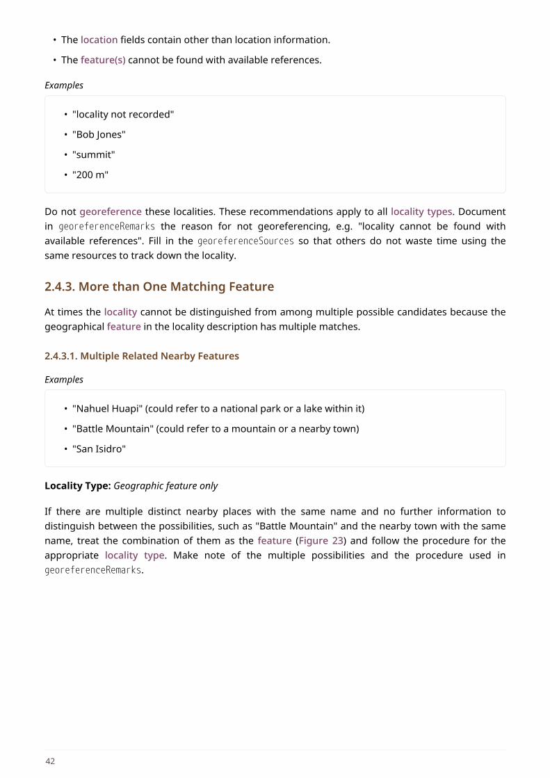
• The location fields contain other than location information.

• The feature(s) cannot be found with available references.

Examples

• "locality not recorded"

• "Bob Jones"

• "summit"

• "200 m"

Do not georeference these localities. These recommendations apply to all locality types. Documentin georeferenceRemarks the reason for not georeferencing, e.g. "locality cannot be found withavailable references". Fill in the georeferenceSources so that others do not waste time using thesame resources to track down the locality.

2.4.3. More than One Matching Feature

At times the locality cannot be distinguished from among multiple possible candidates because thegeographical feature in the locality description has multiple matches.

2.4.3.1. Multiple Related Nearby Features

Examples

• "Nahuel Huapi" (could refer to a national park or a lake within it)

• "Battle Mountain" (could refer to a mountain or a nearby town)

• "San Isidro"

Locality Type: Geographic feature only

If there are multiple distinct nearby places with the same name and no further information todistinguish between the possibilities, such as "Battle Mountain" and the nearby town with the samename, treat the combination of them as the feature (Figure 23) and follow the procedure for theappropriate locality type. Make note of the multiple possibilities and the procedure used ingeoreferenceRemarks.

42

Figure 23. The boundaries for two distinct nearby features with the same name, with center c, corrected center a,and geographic radial b covering the combination of both possible interpretations of the locality.

2.4.3.2. Multiple Unrelated Features

Examples

• "Laguna Blanca" (could refer to distinct lagoons or municipalities in at least five differentcountries)

• "Washington Street" (could refer to multiple streets in different places)

Do not georeference. Document in georeferenceRemarks the reason for not georeferencing, e.g."there are multiple possible unrelated features matching the one in the locality description".

2.4.4. Demonstrably Inconsistent

The locality description contains irreconcilable inconsistencies – assertions that can not all besimultaneously true. Do not georeference these localities. Document in georeferenceRemarks thereason for not georeferencing, e.g. "locality contains irreconcilable inconsistencies".

A common source of inconsistency occurs when the locality description does not match thegeopolitical subdivision of which it is supposed to be a part (e.g. "Missoula County, Idaho"). Elevationis another possible source of inconsistency, especially since elevation data are notoriously inaccurate(see Elevation in Georeferencing Best Practices (Chapman & Wieczorek 2020)). It is difficult to knowwhich part of the locality is the one in error and a risk to judge that one part of the descriptionshould take precedence over another.

43

Examples

• "Sonoma County side of the Gualala River, Mendocino County" (where the river runsbetween the counties mentioned)

• "10 mi W of Bakersfield, 6000 ft" (There is no place anywhere near 10 mi W of Bakersfield atan elevation of 6000 ft)

• "5 mi N of Delano, Kern Co." (5 mi N would put the locality in Tulare Co.)

Do not georeference. Rather than determine coordinates for such localities, annotate the locality ingeoreferenceRemarks with the nature of the inconsistency (e.g. "Missoula County not in Idaho") andrefer the locality to the source institution for reconciliation.

2.4.5. Cultivated or Captive

The locality is recorded in association with a captive animal, a cultivated plant or some other non-natural occurrence. The locality cited is often that of a zoo, aquarium, botanical garden, etc. (seeDealing with Non-natural Occurrences in Georeferencing Best Practices (Chapman & Wieczorek2020).

The fact that an organism is recorded in a place out of its known or assumednatural distribution range does not constitute a problem from the point of view oflocating that organism. Therefore, the determination of a georeference should nothave any issues aside from those exclusively derived from the locality descriptionitself (as seen for other cases above). This kind of information should instead becaptured in the Darwin Core term degreeOfEstablishment.

If you are georeferencing based on location information only, and not together withthe associated occurrence records, you may not have an easy way to capture otherkinds of information (e.g. provenance, dates, degree of establishment, etc.). Inthese cases, it is recommended to amend the original occurrence records thatcontain the given locality to avoid any loss of information.

Examples

• "lab born, University of Oregon"

• "bait shop"

• "Cultivated in Botanic Gardens from seed obtained from Bourke, NSW."

• "San Diego Wild Animal Park"

Georeference the locality normally based on the locality type and feature. Retain the location (e.g.zoo) along with its georeference, as for other localities in this Guide, but be sure to record the natureof its provenance (cultivated, captive, washed ashore, etc.) in the Darwin Core termdegreeOfEstablishment.

44

GlossaryThe purpose of this glossary is to describe important concepts in accordance with the intendedmeaning in this document, the associated Georeferencing Best Practices (Chapman & Wieczorek2020) and the Georeferencing Calculator Manual (Bloom et al. 2020). These concepts are treated inbroader contexts in many other sources. We have adapted the terms presented here from manysources including Wikipedia (as of November, 2019), the ESRI Dictionary (as of November, 2019) (ESRIn.d.), and various articles within Kemp 2008.

accuracy

The closeness of an estimated value (for example, measured or computed) to a standard oraccepted ("true") value. Antonym: inaccuracy Compare error, bias, precision, false precision anduncertainty.

"The true value is not known, but only estimated, the accuracy of the measuredquantity is also unknown. Therefore, accuracy of coordinate information can onlybe estimated." (Geodetic Survey Division 1996, FGDC 1998).

bathymetry

1. The measure of depth of water in oceans, seas and lakes.

2. The shapes of underwater terrains, including underwater topography and sea floor mapping.

boundary

The spatial divide between what is inside a location and what is outside of it.

bounding box

An area defined by the coordinates of two diagonally opposite corners of a polygon, where thosetwo corners define the north-south and east-west extremes of the area contained within.

coordinate format

The format in which coordinates are encoded, such as "decimal degrees", "degrees minutesseconds", "degrees decimal minutes", or Universal Transverse Mercator UTM.

coordinate precision

The fraction of a degree corresponding to the number of significant digits in the sourcecoordinates. For example, if the coordinates are reported to the nearest minute, the precision is1/3600th (0.00027778) of a degree; if a decimal degree is reported to two decimal places, theprecision is 0.01 of a degree.

coordinate reference system

(also spatial reference system) A coordinate system defined in relation to a standard reference ordatum.

coordinate system

A geometric system that defines the nature and relationship of the coordinates it uses to uniquelydefine positions. Examples include the geographic coordinate system and the UniversalTransverse Mercator UTM coordinate system.

45

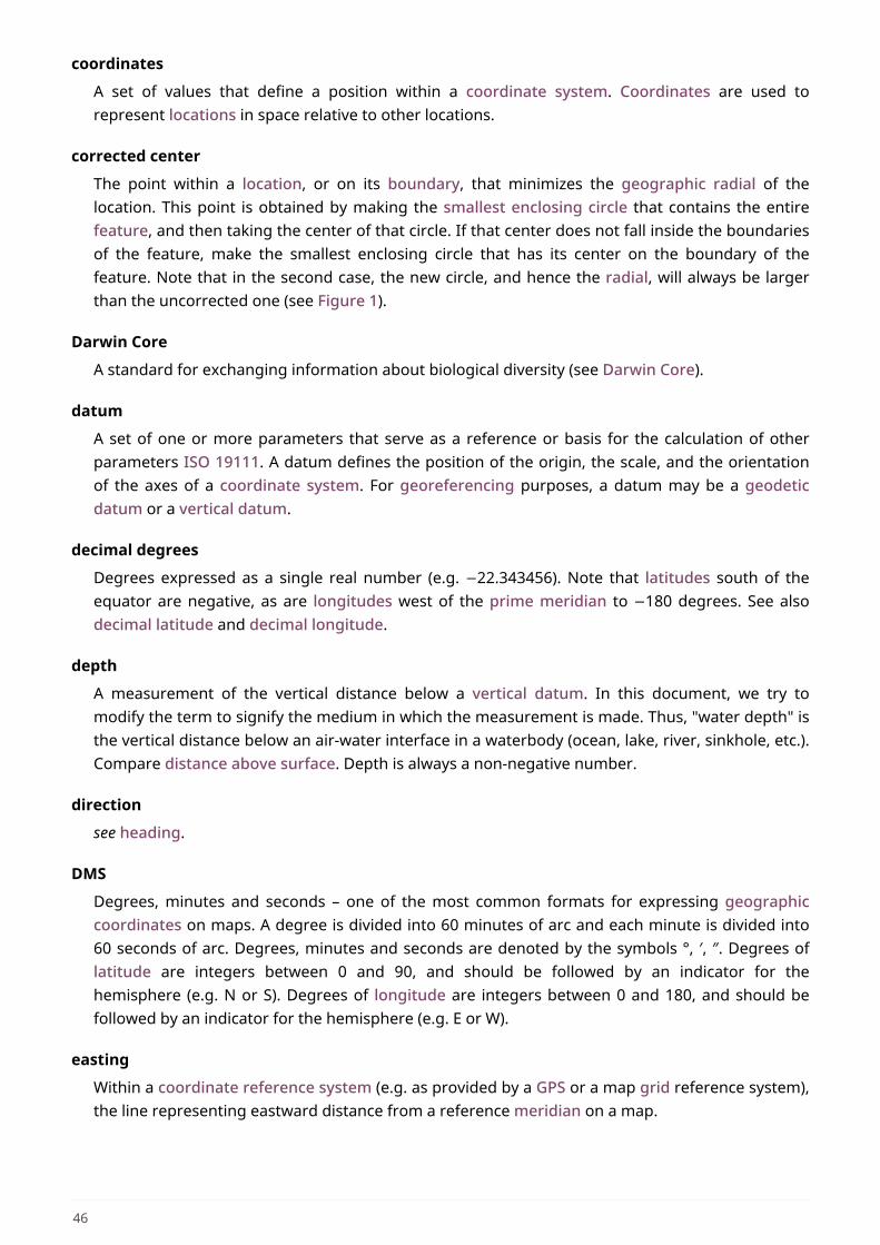
coordinates

A set of values that define a position within a coordinate system. Coordinates are used torepresent locations in space relative to other locations.

corrected center

The point within a location, or on its boundary, that minimizes the geographic radial of thelocation. This point is obtained by making the smallest enclosing circle that contains the entirefeature, and then taking the center of that circle. If that center does not fall inside the boundariesof the feature, make the smallest enclosing circle that has its center on the boundary of thefeature. Note that in the second case, the new circle, and hence the radial, will always be largerthan the uncorrected one (see Figure 1).

Darwin Core

A standard for exchanging information about biological diversity (see Darwin Core).

datum

A set of one or more parameters that serve as a reference or basis for the calculation of otherparameters ISO 19111. A datum defines the position of the origin, the scale, and the orientationof the axes of a coordinate system. For georeferencing purposes, a datum may be a geodeticdatum or a vertical datum.

decimal degrees

Degrees expressed as a single real number (e.g. −22.343456). Note that latitudes south of theequator are negative, as are longitudes west of the prime meridian to −180 degrees. See alsodecimal latitude and decimal longitude.

depth

A measurement of the vertical distance below a vertical datum. In this document, we try tomodify the term to signify the medium in which the measurement is made. Thus, "water depth" isthe vertical distance below an air-water interface in a waterbody (ocean, lake, river, sinkhole, etc.).Compare distance above surface. Depth is always a non-negative number.

direction

see heading.

DMS

Degrees, minutes and seconds – one of the most common formats for expressing geographiccoordinates on maps. A degree is divided into 60 minutes of arc and each minute is divided into60 seconds of arc. Degrees, minutes and seconds are denoted by the symbols °, ′, ″. Degrees oflatitude are integers between 0 and 90, and should be followed by an indicator for thehemisphere (e.g. N or S). Degrees of longitude are integers between 0 and 180, and should befollowed by an indicator for the hemisphere (e.g. E or W).

easting

Within a coordinate reference system (e.g. as provided by a GPS or a map grid reference system),the line representing eastward distance from a reference meridian on a map.

46

elevation

A measurement of the vertical distance of a land or water surface above a vertical datum. Onmaps, the reference datum is generally some interpretation of mean sea level or the geoid, whilein devices using GPS/GNSS, the reference datum is the ellipsoid of the geodetic datum to whichthe GPS unit is configured, though the device may make corrections to report the elevation abovemean sea level or the geoid. Elevations that are above a reference point should be expressed aspositive numbers, while those below should be negative. Compare depth, distance above surface,and altitude.

ellipsoid

A three-dimensional, closed geometric shape, all planar sections of which are ellipses or circles.An ellipsoid has three independent axes. If an ellipsoid is made by rotating an ellipse about one ofits axes, then two axes of the ellipsoid are the same, and it is called an ellipsoid of revolution.When used to represent a model of the earth, the ellipsoid is an oblate ellipsoid of revolutionmade by rotating an ellipse about its minor axis.

entry point

The entry point on the surface of the ocean or lake where a diver enters the water and from whichall activities are measured. See illustration in Georeferencing Best Practices (Chapman & Wieczorek2020).

error

The difference between a computed, estimated, or measured value and the accepted true,specified, or theoretically correct value. It encompasses both the imprecision of a measurementand its inaccuracies. Error can be either random or systematic. If the error is systematic, it iscalled "bias". Compare accuracy, bias, precision, false precision and uncertainty.

extent

The entire space within the boundary a location actually represents. The extent can be a volume,an area, or a distance.

feature

An object of observation, measurement, or reference that can be represented spatially. Oftencategorized into "feature types" (e.g. mountain, road, populated place, etc.) and given names forspecific instances (e.g. "Mount Everest", "Ruta 40", "Istanbul"), which are also sometimes referredto as "named places", "place names" or "toponyms".

gazetteer

An index of geographical features and their locations, often with geographic coordinates.

geocode

The process (verb) or product (noun) of determining the coordinates for a street address. It is alsosometimes used as a synonym for georeference.

geographic boundary

The representation in geographic coordinates of a vertical projection of a boundary onto a modelof the surface of the Earth.

47

geographic center

The midpoint of the extremes of latitude and longitude of a feature. Geographic centers arerelatively easy to determine, but they generally do not correspond to the center obtained by aleast circumscribing circle. For that reason it is not recommended to use a geographic center forany application in georeferencing. Compare corrected center.

geographic coordinates

A measurement of a location on the Earth’s surface expressed as latitude and longitude.

geographic radial

The distance from the corrected center of a location to the furthest point on the geographicboundary of that location. The geographical radial is what contributes to calculations of themaximum uncertainty distance using the point-radius georeferencing method. The termgeographic radial, as defined here, replaces its equivalent "extent" used in the early versions ofthis Quick Reference Guide and related documents.

geometry

The measures and properties of points, lines, and surfaces. Geometry is used to represent thegeographic component of locations.

georeference

The process (verb) or product (noun) of interpreting a locality description into a spatiallymappable representation using a georeferencing method. Compare with geocode. The usagehere is distinct from the concept of georeferencing satellite and other imagery (known asgeorectification).

georeferencing method

The theory, including a set of rules, general procedures and expected outcomes, meant toproduce a specific type of spatial representation of a locality.

georeferencing protocol

The set of specific documented steps that can be applied to produce a spatial representation of alocality, following one or more georeferencing methods.

GPS

Global Positioning System, a satellite-based system used for determining positions on or near theEarth. Orbiting satellites transmit radio signals that allow a receiver to calculate its own locationas coordinates and elevation, sometimes with accuracy estimates. See also GNSS of which GPS isone example. See also GPS (receiver).

GPS (receiver)

The colloquial term used to refer to both GPS and GNSS receivers (including those in smartphonesand cameras). A GPS or GNSS receiver is an instrument which, in combination with an inbuilt orseparate antenna, is able to receive and interpret radio signals from GNSS satellites and translatethem into geographic coordinates.

grid

A network or array of evenly spaced orthogonal lines used to organize space into partitions. Often

48

these are superimposed on a map and used for reference, such as Universal Transverse MercatorUTM grid.

ground zero

The location on the land surface directly above a radiolocation point in a cave where the magneticradiation lines are vertical. See illustration in Georeferencing Best Practices (Chapman & Wieczorek2020).

heading

Compass direction such as east or northwest, or sometimes given as degrees clockwise fromnorth. Usually used in conjunction with offset to give a distance and direction from a feature.

latitude

The angular distance of a point north or south of the equator.

locality

The verbal representation of a location, also sometimes called locality description.

locality clause

A part of a locality description that can be categorized into one of the locality types, to which aspecific georeferencing protocol can be applied.

locality type

A category applied to a locality clause that determines the specific georeferencing protocol thatshould be used.

location

A physical space that can be positioned and oriented relative to a reference point, and potentiallydescribed in a natural language locality description. In georeferencing, a location can havedistinct representations based on distinct rules of interpretation, each of which is embodied in ageoreferencing method.

longitude

The angular distance of a point east or west of a prime meridian at a given latitude.

meridian

A line on the surface of the Earth where all of the locations have the same longitude. Compareantimeridian and prime meridian.

northing

Within a coordinate reference system (e.g. as provided by a GPS or a map grid reference system),the line representing northward distance from a reference latitude.

offset

A displacement from a reference location. Usually used in conjunction with heading to give adistance and direction from a feature.

49

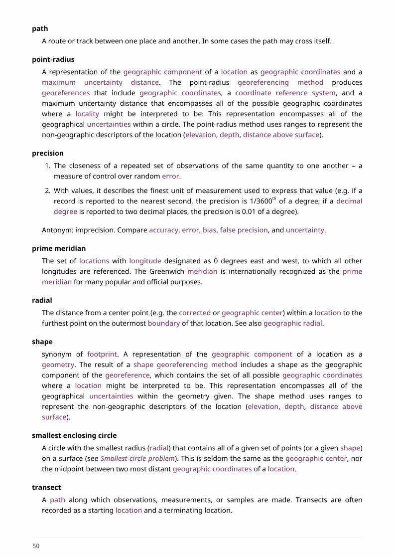
path

A route or track between one place and another. In some cases the path may cross itself.

point-radius

A representation of the geographic component of a location as geographic coordinates and amaximum uncertainty distance. The point-radius georeferencing method producesgeoreferences that include geographic coordinates, a coordinate reference system, and amaximum uncertainty distance that encompasses all of the possible geographic coordinateswhere a locality might be interpreted to be. This representation encompasses all of thegeographical uncertainties within a circle. The point-radius method uses ranges to represent thenon-geographic descriptors of the location (elevation, depth, distance above surface).

precision

1. The closeness of a repeated set of observations of the same quantity to one another – ameasure of control over random error.

2. With values, it describes the finest unit of measurement used to express that value (e.g. if arecord is reported to the nearest second, the precision is 1/3600th of a degree; if a decimaldegree is reported to two decimal places, the precision is 0.01 of a degree).

Antonym: imprecision. Compare accuracy, error, bias, false precision, and uncertainty.

prime meridian

The set of locations with longitude designated as 0 degrees east and west, to which all otherlongitudes are referenced. The Greenwich meridian is internationally recognized as the primemeridian for many popular and official purposes.

radial

The distance from a center point (e.g. the corrected or geographic center) within a location to thefurthest point on the outermost boundary of that location. See also geographic radial.

shape

synonym of footprint. A representation of the geographic component of a location as ageometry. The result of a shape georeferencing method includes a shape as the geographiccomponent of the georeference, which contains the set of all possible geographic coordinateswhere a location might be interpreted to be. This representation encompasses all of thegeographical uncertainties within the geometry given. The shape method uses ranges torepresent the non-geographic descriptors of the location (elevation, depth, distance abovesurface).

smallest enclosing circle

A circle with the smallest radius (radial) that contains all of a given set of points (or a given shape)on a surface (see Smallest-circle problem). This is seldom the same as the geographic center, northe midpoint between two most distant geographic coordinates of a location.

transect

A path along which observations, measurements, or samples are made. Transects are oftenrecorded as a starting location and a terminating location.

50

uncertainty

A measure of the incompleteness of one’s knowledge or information about an unknown quantitywhose true value could be established if complete knowledge and a perfect measuring devicewere available (Cullen & Frey 1999). Georeferencing methods codify how to incorporateuncertainties from a variety of sources (including accuracy and precision) in the interpretation ofa location. Compare accuracy, error, bias, precision, and false precision.

Universal Transverse Mercator UTM

A standardized coordinate system based on a metric rectangular grid system and a division of theEarth into sixty 6-degree longitudinal zones. The scope of UTM covers from 84° N to 80° S. (SeeUniversal Transverse Mercator (UTM) Coordinates in Georeferencing Best Practices (Chapman &Wieczorek 2020)).

51

AcknowledgementsMany people have contributed ideas to this document and its precursors, either directly or indirectlythrough discussions at meetings, publications, or in email correspondence. We refer you to theearlier document for those we acknowledged there.

The people we would like to particularly acknowledge for this document include Arturo H. Ariño,Ricardo Ortiz Gallego, Quentin Groom, Kyle Kopas, Erica Krimmel, and Nelson Rios. We would furtherlike to acknowledge the staff at the GBIF Secretariat, especially Laura Russell, Kyle Copas, andMatthew Blissett who provided support for the project in which this document was solicited.

References▪ Bloom DA, Wieczorek JR, Zermoglio PF (2020) Georeferencing Calculator Manual. Copenhagen:

GBIF Secretariat. https://doi.org/10.35035/gdwq-3v93

▪ Chapman AD & Wieczorek J (2020) Georeferencing Best Practices. Copenhagen: GBIF Secretariat.https://doi.org/10.15468/doc-gg7h-s853

▪ Chapman AD, Muñoz MES & Koch I (2005) Environmental Information: Placing BiodiversityPhenomena in an Ecological and Environmental Context. Biodiversity Informatics 2: 24-41.https://doi.org/10.17161/bi.v2i0.5

▪ Cullen AC & Frey HC (1999) Probabilistic Techniques in Exposure Assessment: A Handbook forDealing with Variability and Uncertainty in Models and Inputs. New York: Plenum Press.

▪ ESRI (n.d.) GIS Dictionary. https://support.esri.com/en/other-resources/gis-dictionary/browse/

▪ FGDC (1998) Geospatial Positioning Accuracy Standards, Part 3: National Standards for SpatialData Accuracy. FGDC-STD-007.3-1998. Reston, Va., USA. https://www.fgdc.gov/standards/projects/accuracy/part3/chapter3

▪ Frazier C, Neville T, Giermakowski JT & Racz G (2004) The INRAM Protocol for GeoreferencingBiological Museum Specimen Records, version 1.3. Zenodo. http://doi.org/10.5281/zenodo.3235003

▪ Geodetic Survey Division (1996) Accuracy Standards for Positioning, Version 1.0: Ottawa, Canada:Natural Resources Canada. ftp://glonass-center.ru/REPORTS/OLD/NRCAN/Accuracy_Standards.pdf

▪ Kemp KK (2008) Encyclopedia of Geographic Information Science. Los Angeles: Sage Publications.https://doi.org/10.4135/9781412953962

▪ Spencer C, Yamamoto K, Fang J, Constable H, Koo M, & Wieczorek J (2008) Georeferencing forDummies. http://georeferencing.org/docs/georeffordummy.xls

▪ TDWG (2018) Darwin Core quick reference guide. Biodiversity Information Standards (TDWG).https://dwc.tdwg.org/terms/

▪ Wieczorek C & Wieczorek J (2020) Georeferencing Calculator, version 20191217en. Rauthiflor LLC.http://georeferencing.org/georefcalculator/gc.html

▪ Wieczorek J (2001) MaNIS/HerpNET/ORNIS Georeferencing Guidelines. University of California,Berkeley: Museum of Vertebrate Zoology. http://georeferencing.org/georefcalculator/docs/

52

GeorefGuide.html

▪ Wieczorek J, Bloom D, Constable H, Fang J, Koo M, Spencer C & Yamamo K (2012) GeoreferencingQuick Reference Guide, version 2012-10-08. http://www.herpnet.org/herpnet/documents/GeoreferencingQuickGuide.pdf

▪ Wieczorek J & Bloom DA (2015) Manual for the Georeferencing Calculator. University of California,Berkeley: Museum of Vertebrate Zoology. http://georeferencing.org/gci2/docs/GeoreferencingCalculatorManualv2.html

▪ Wieczorek J, Guo Q & Hijmans R (2004) The point-radius method for georeferencing localitydescriptions and calculating associated uncertainty. International Journal of GeographicalInformation Science. 18: 745-767. https://doi.org/10.1080/13658810412331280211

53

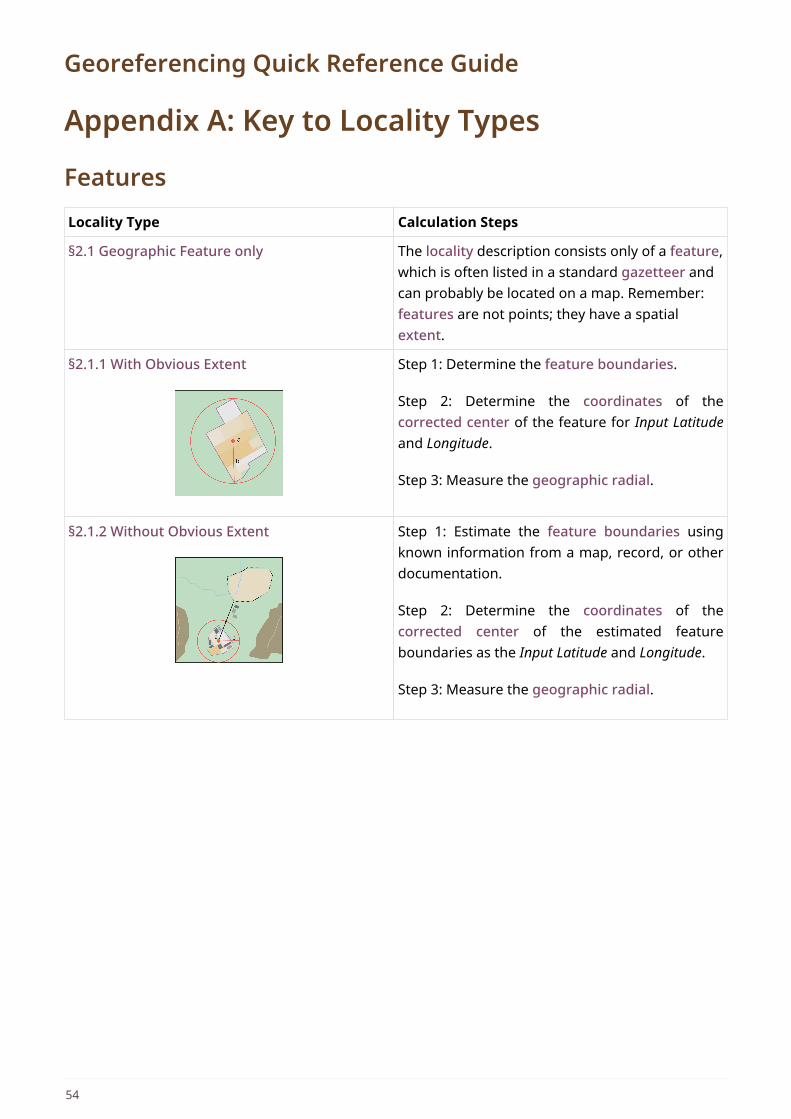
Georeferencing Quick Reference Guide

Appendix A: Key to Locality Types

FeaturesLocality Type Calculation Steps

§2.1 Geographic Feature only The locality description consists only of a feature,which is often listed in a standard gazetteer andcan probably be located on a map. Remember:features are not points; they have a spatialextent.

§2.1.1 With Obvious Extent Step 1: Determine the feature boundaries.

Step 2: Determine the coordinates of thecorrected center of the feature for Input Latitudeand Longitude.

Step 3: Measure the geographic radial.

§2.1.2 Without Obvious Extent Step 1: Estimate the feature boundaries usingknown information from a map, record, or otherdocumentation.

Step 2: Determine the coordinates of thecorrected center of the estimated featureboundaries as the Input Latitude and Longitude.

Step 3: Measure the geographic radial.

54

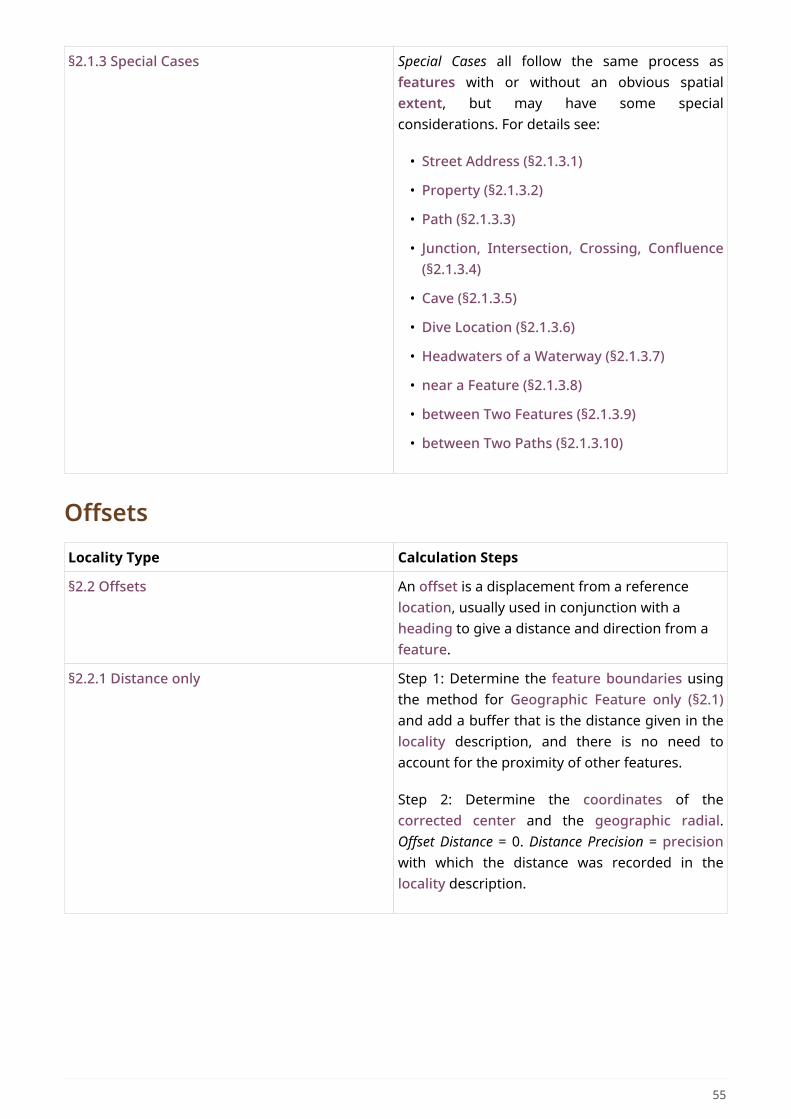
§2.1.3 Special Cases Special Cases all follow the same process asfeatures with or without an obvious spatialextent, but may have some specialconsiderations. For details see:

• Street Address (§2.1.3.1)

• Property (§2.1.3.2)

• Path (§2.1.3.3)

• Junction, Intersection, Crossing, Confluence(§2.1.3.4)

• Cave (§2.1.3.5)

• Dive Location (§2.1.3.6)

• Headwaters of a Waterway (§2.1.3.7)

• near a Feature (§2.1.3.8)

• between Two Features (§2.1.3.9)

• between Two Paths (§2.1.3.10)

OffsetsLocality Type Calculation Steps

§2.2 Offsets An offset is a displacement from a referencelocation, usually used in conjunction with aheading to give a distance and direction from afeature.

§2.2.1 Distance only Step 1: Determine the feature boundaries usingthe method for Geographic Feature only (§2.1)and add a buffer that is the distance given in thelocality description, and there is no need toaccount for the proximity of other features.

Step 2: Determine the coordinates of thecorrected center and the geographic radial.Offset Distance = 0. Distance Precision = precisionwith which the distance was recorded in thelocality description.

55

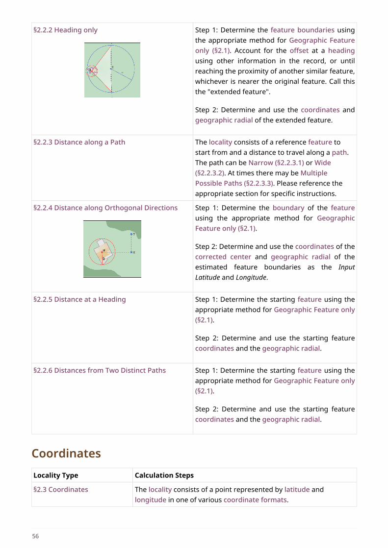
§2.2.2 Heading only Step 1: Determine the feature boundaries usingthe appropriate method for Geographic Featureonly (§2.1). Account for the offset at a headingusing other information in the record, or untilreaching the proximity of another similar feature,whichever is nearer the original feature. Call thisthe "extended feature".

Step 2: Determine and use the coordinates andgeographic radial of the extended feature.

§2.2.3 Distance along a Path The locality consists of a reference feature tostart from and a distance to travel along a path.The path can be Narrow (§2.2.3.1) or Wide(§2.2.3.2). At times there may be MultiplePossible Paths (§2.2.3.3). Please reference theappropriate section for specific instructions.

§2.2.4 Distance along Orthogonal Directions Step 1: Determine the boundary of the featureusing the appropriate method for GeographicFeature only (§2.1).

Step 2: Determine and use the coordinates of thecorrected center and geographic radial of theestimated feature boundaries as the InputLatitude and Longitude.

§2.2.5 Distance at a Heading Step 1: Determine the starting feature using theappropriate method for Geographic Feature only(§2.1).

Step 2: Determine and use the starting featurecoordinates and the geographic radial.

§2.2.6 Distances from Two Distinct Paths Step 1: Determine the starting feature using theappropriate method for Geographic Feature only(§2.1).

Step 2: Determine and use the starting featurecoordinates and the geographic radial.

CoordinatesLocality Type Calculation Steps

§2.3 Coordinates The locality consists of a point represented by latitude andlongitude in one of various coordinate formats.

56

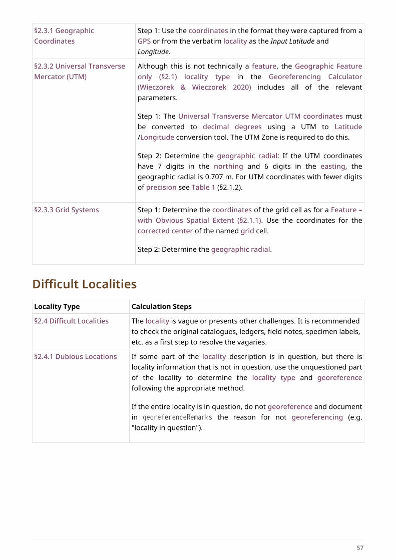
§2.3.1 GeographicCoordinates

Step 1: Use the coordinates in the format they were captured from aGPS or from the verbatim locality as the Input Latitude andLongitude.

§2.3.2 Universal TransverseMercator (UTM)

Although this is not technically a feature, the Geographic Featureonly (§2.1) locality type in the Georeferencing Calculator(Wieczorek & Wieczorek 2020) includes all of the relevantparameters.

Step 1: The Universal Transverse Mercator UTM coordinates mustbe converted to decimal degrees using a UTM to Latitude/Longitude conversion tool. The UTM Zone is required to do this.

Step 2: Determine the geographic radial: If the UTM coordinateshave 7 digits in the northing and 6 digits in the easting, thegeographic radial is 0.707 m. For UTM coordinates with fewer digitsof precision see Table 1 (§2.1.2).

§2.3.3 Grid Systems Step 1: Determine the coordinates of the grid cell as for a Feature –with Obvious Spatial Extent (§2.1.1). Use the coordinates for thecorrected center of the named grid cell.

Step 2: Determine the geographic radial.

Difficult LocalitiesLocality Type Calculation Steps

§2.4 Difficult Localities The locality is vague or presents other challenges. It is recommendedto check the original catalogues, ledgers, field notes, specimen labels,etc. as a first step to resolve the vagaries.

§2.4.1 Dubious Locations If some part of the locality description is in question, but there islocality information that is not in question, use the unquestioned partof the locality to determine the locality type and georeferencefollowing the appropriate method.

If the entire locality is in question, do not georeference and documentin georeferenceRemarks the reason for not georeferencing (e.g."locality in question").

57

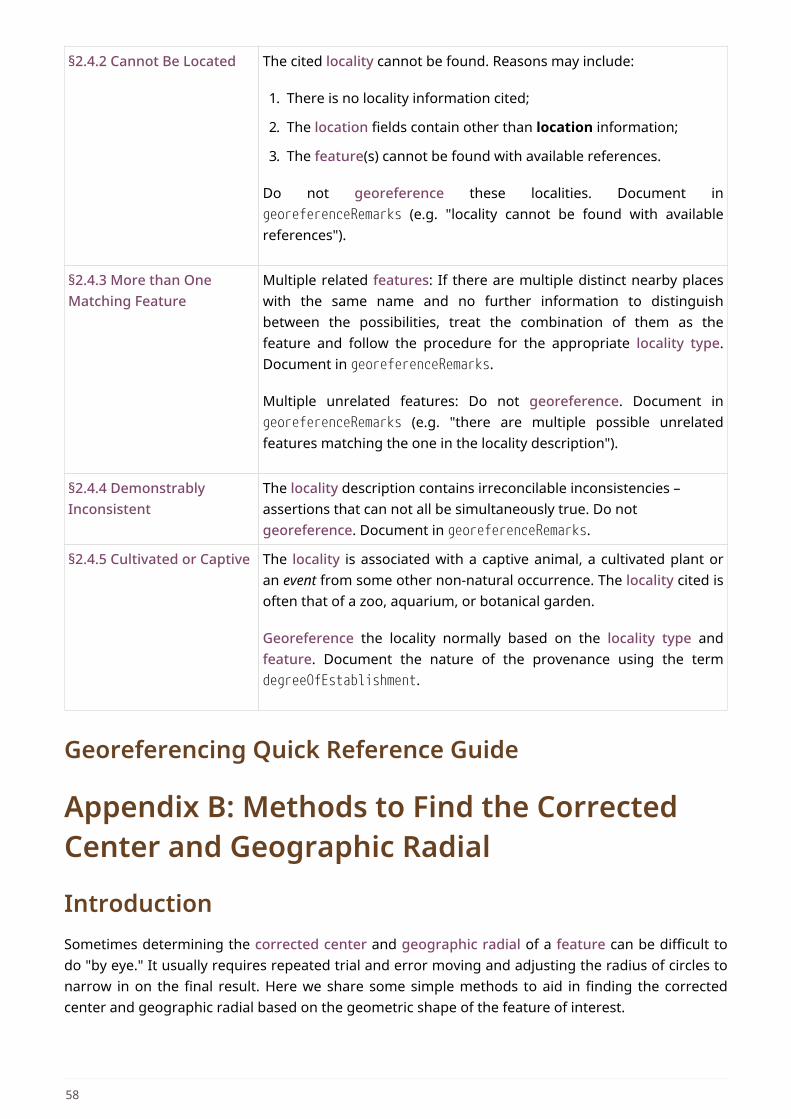
§2.4.2 Cannot Be Located The cited locality cannot be found. Reasons may include:

1. There is no locality information cited;

2. The location fields contain other than location information;

3. The feature(s) cannot be found with available references.

Do not georeference these localities. Document ingeoreferenceRemarks (e.g. "locality cannot be found with availablereferences").

§2.4.3 More than OneMatching Feature

Multiple related features: If there are multiple distinct nearby placeswith the same name and no further information to distinguishbetween the possibilities, treat the combination of them as thefeature and follow the procedure for the appropriate locality type.Document in georeferenceRemarks.

Multiple unrelated features: Do not georeference. Document ingeoreferenceRemarks (e.g. "there are multiple possible unrelatedfeatures matching the one in the locality description").

§2.4.4 DemonstrablyInconsistent

The locality description contains irreconcilable inconsistencies –assertions that can not all be simultaneously true. Do notgeoreference. Document in georeferenceRemarks.

§2.4.5 Cultivated or Captive The locality is associated with a captive animal, a cultivated plant oran event from some other non-natural occurrence. The locality cited isoften that of a zoo, aquarium, or botanical garden.

Georeference the locality normally based on the locality type andfeature. Document the nature of the provenance using the termdegreeOfEstablishment.

Georeferencing Quick Reference Guide

Appendix B: Methods to Find the CorrectedCenter and Geographic Radial

IntroductionSometimes determining the corrected center and geographic radial of a feature can be difficult todo "by eye." It usually requires repeated trial and error moving and adjusting the radius of circles tonarrow in on the final result. Here we share some simple methods to aid in finding the correctedcenter and geographic radial based on the geometric shape of the feature of interest.

58

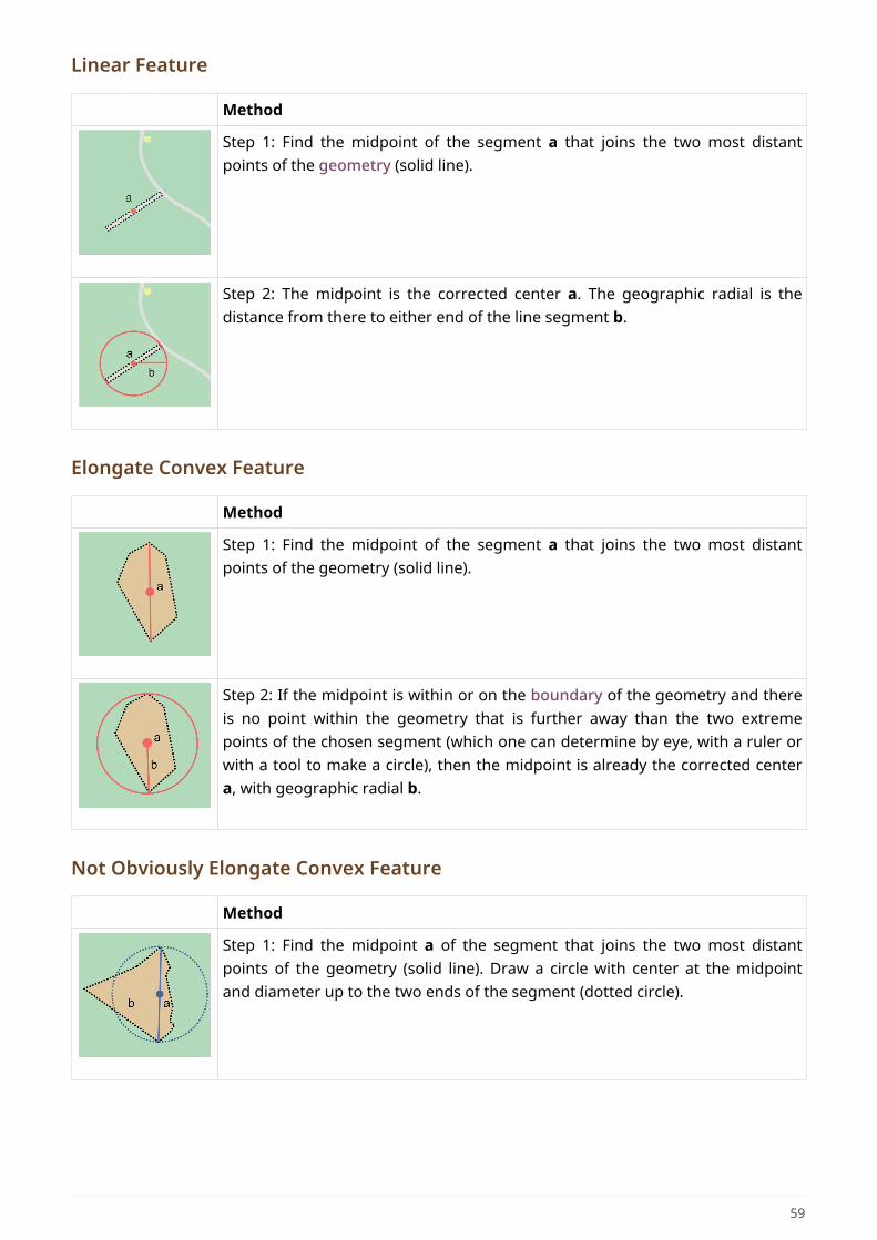
Linear Feature

Method

Step 1: Find the midpoint of the segment a that joins the two most distantpoints of the geometry (solid line).

Step 2: The midpoint is the corrected center a. The geographic radial is thedistance from there to either end of the line segment b.

Elongate Convex Feature

Method

Step 1: Find the midpoint of the segment a that joins the two most distantpoints of the geometry (solid line).

Step 2: If the midpoint is within or on the boundary of the geometry and thereis no point within the geometry that is further away than the two extremepoints of the chosen segment (which one can determine by eye, with a ruler orwith a tool to make a circle), then the midpoint is already the corrected centera, with geographic radial b.

Not Obviously Elongate Convex Feature

Method

Step 1: Find the midpoint a of the segment that joins the two most distantpoints of the geometry (solid line). Draw a circle with center at the midpointand diameter up to the two ends of the segment (dotted circle).

59

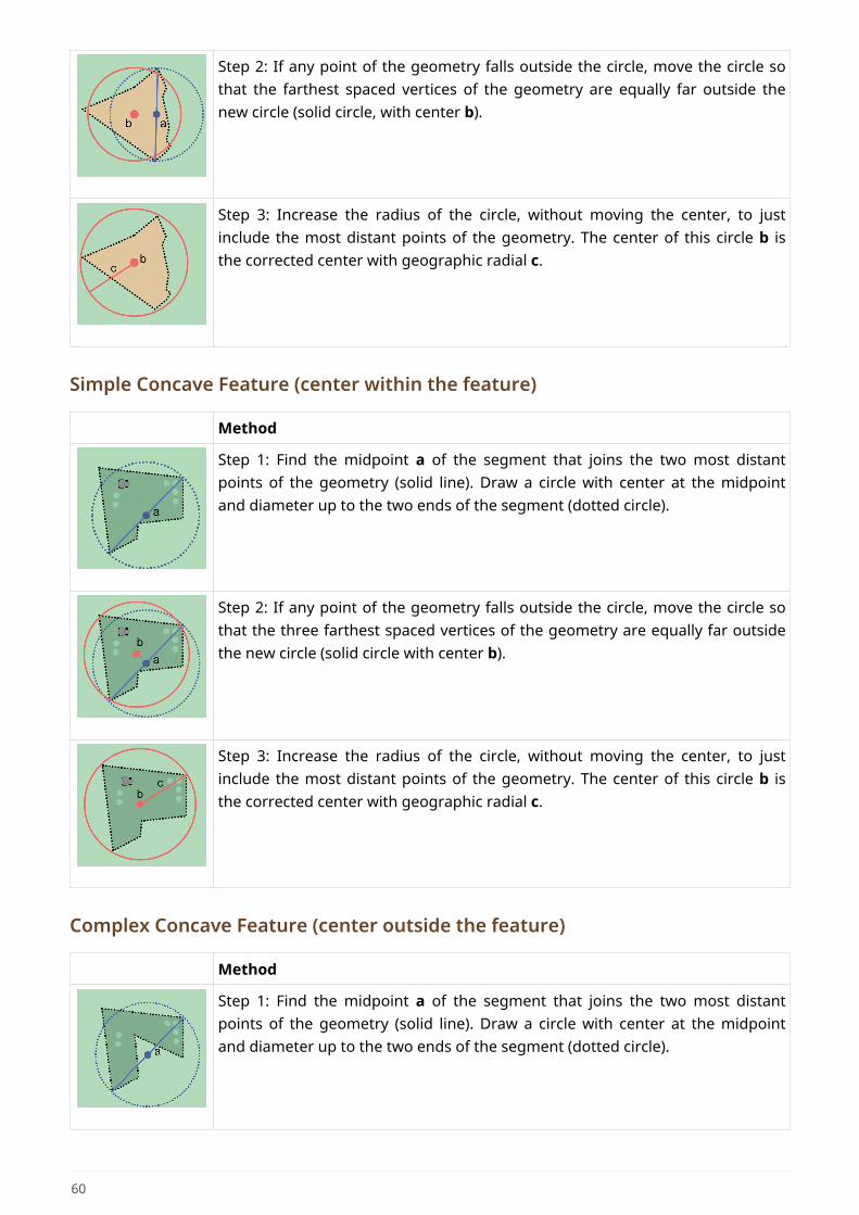
Step 2: If any point of the geometry falls outside the circle, move the circle sothat the farthest spaced vertices of the geometry are equally far outside thenew circle (solid circle, with center b).

Step 3: Increase the radius of the circle, without moving the center, to justinclude the most distant points of the geometry. The center of this circle b isthe corrected center with geographic radial c.

Simple Concave Feature (center within the feature)

Method

Step 1: Find the midpoint a of the segment that joins the two most distantpoints of the geometry (solid line). Draw a circle with center at the midpointand diameter up to the two ends of the segment (dotted circle).

Step 2: If any point of the geometry falls outside the circle, move the circle sothat the three farthest spaced vertices of the geometry are equally far outsidethe new circle (solid circle with center b).

Step 3: Increase the radius of the circle, without moving the center, to justinclude the most distant points of the geometry. The center of this circle b isthe corrected center with geographic radial c.

Complex Concave Feature (center outside the feature)

Method

Step 1: Find the midpoint a of the segment that joins the two most distantpoints of the geometry (solid line). Draw a circle with center at the midpointand diameter up to the two ends of the segment (dotted circle).

60

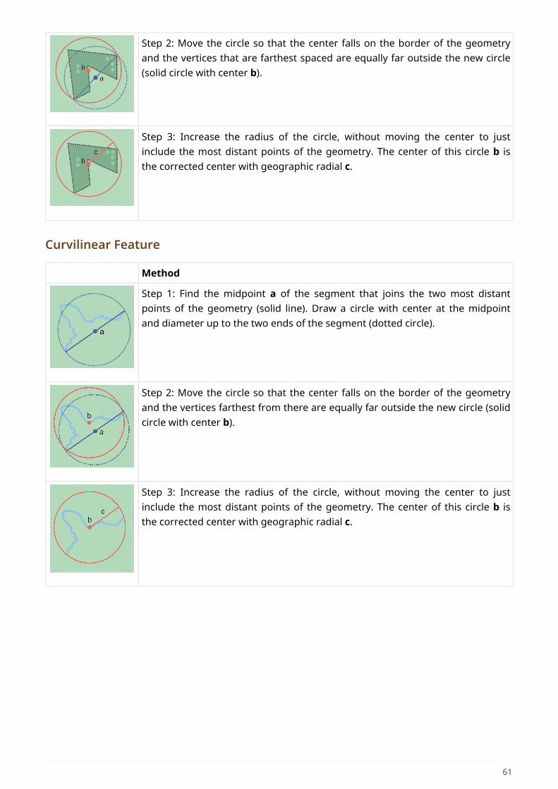
Step 2: Move the circle so that the center falls on the border of the geometryand the vertices that are farthest spaced are equally far outside the new circle(solid circle with center b).

Step 3: Increase the radius of the circle, without moving the center to justinclude the most distant points of the geometry. The center of this circle b isthe corrected center with geographic radial c.

Curvilinear Feature

Method

Step 1: Find the midpoint a of the segment that joins the two most distantpoints of the geometry (solid line). Draw a circle with center at the midpointand diameter up to the two ends of the segment (dotted circle).

Step 2: Move the circle so that the center falls on the border of the geometryand the vertices farthest from there are equally far outside the new circle (solidcircle with center b).

Step 3: Increase the radius of the circle, without moving the center to justinclude the most distant points of the geometry. The center of this circle b isthe corrected center with geographic radial c.

61