geostatistical approaches for incorporating elevation into ...geostatistical approaches for...

Geostatistical approaches for incorporating elevation into thespatial interpolation of rainfall

P. Goovaerts*

Department of Civil and Environmental Engineering, The University of Michigan, Ann Arbor, MI 48109-2125, USA

Received 11 February 1999; received in revised form 11 November 1999; accepted 16 December 1999

Abstract

This paper presents three multivariate geostatistical algorithms for incorporating a digital elevation model into the spatialprediction of rainfall: simple kriging with varying local means; kriging with an external drift; and colocated cokriging. Thetechniques are illustrated using annual and monthly rainfall observations measured at 36 climatic stations in a 5000 km2 regionof Portugal. Cross validation is used to compare the prediction performances of the three geostatistical interpolation algorithmswith the straightforward linear regression of rainfall against elevation and three univariate techniques: the Thiessen polygon;inverse square distance; and ordinary kriging.

Larger prediction errors are obtained for the two algorithms (inverse square distance, Thiessen polygon) that ignore both theelevation and rainfall records at surrounding stations. The three multivariate geostatistical algorithms outperform other inter-polators, in particular the linear regression, which stresses the importance of accounting for spatially dependent rainfallobservations in addition to the colocated elevation. Last, ordinary kriging yields more accurate predictions than linear regres-sion when the correlation between rainfall and elevation is moderate (less than 0.75 in the case study).q 2000 Elsevier ScienceB.V. All rights reserved.

Keywords: Rainfall; DEM; Multivariate geostatistics; Kriging

1. Introduction

Measured rainfall data are important to manyproblems in hydrologic analysis and designs. Forexample the ability of obtaining high resolution esti-mates of spatial variability in rainfall fields becomesimportant for identification of locally intense stormswhich could lead to floods and especially to flashfloods. The accurate estimation of the spatial distribu-tion of rainfall requires a very dense network ofinstruments, which entails large installation andoperational costs. Also, vandalism or the failure of

the observer to make the necessary visit to the gagemay result in even lower sampling density. It is thusnecessary to estimate point rainfall at unrecordedlocations from values at surrounding sites.

A number of methods have been proposed for theinterpolation of rainfall data. The simplest approachconsists of assigning to the unsampled location therecord of the closest gage (Thiessen, 1911). Thismethod amounts at drawing around each gage a poly-gon of influence with the boundaries at a distancehalfway between gage pairs, hence the name Thiessenpolygon for the technique. Although the Thiessenpolygon method is essentially used for estimation ofareal rainfall (McCuen, 1998), it has also been appliedto the interpolation of point measurements (Creutin

Journal of Hydrology 228 (2000) 113–129

0022-1694/00/$ - see front matterq 2000 Elsevier Science B.V. All rights reserved.PII: S0022-1694(00)00144-X

www.elsevier.com/locate/jhydrol

* Tel.: 11-734-936-0141; fax:11-734-763-2275.E-mail address:[email protected] (P. Goovaerts).

and Obled, 1982; Tabios and Salas, 1985; Dirks et al.,1998). In 1972, the US National Weather Service hasdeveloped another method whereby the unknownrainfall depth is estimated as a weighted average ofsurrounding values, the weights being reciprocal tothe square distances from the unsampled location(Bedient and Huber, 1992, p. 25). Like the Thiessenpolygon method, the inverse square distance tech-nique does not allow the hydrologist to considerfactors, such as topography, that can affect the catchat a gage. The isohyetal method (McCuen, 1998,p. 190) is designed to overcome this deficiency. Theidea is to use the location and catch for each gage, aswell as knowledge of the factors affecting thesecatches, to draw lines of equal rainfall depth (isohyets).The amount of rainfall at the unsampled location isthen estimated by interpolation within the isohyets. Alimitation of the technique is that an extensive gagenetwork is required to draw isohyets accurately.

Geostatistics, which is based on the theory ofregionalized variables (Journel and Huijbregts,1978; Goovaerts, 1997, 1999), is increasinglypreferred because it allows one to capitalize on thespatial correlation between neighboring observationsto predict attribute values at unsampled locations.Several authors (Tabios and Salas, 1985; Phillips etal., 1992) have shown that the geostatistical predictiontechnique (kriging) provides better estimates of rain-fall than conventional methods. Recently, Dirks et al.(1998) found that the results depend on the samplingdensity and that, for high-resolution networks (e.g. 13raingages over a 35 km2 area), the kriging methoddoes not show significantly greater predictive skillthan simpler techniques, such as the inverse squaredistance method. Similar results were found byBorga and Vizzaccaro (1997) when they comparedkriging and multiquadratic surface fitting for variousgage densities. In fact, besides providing a measure of

P. Goovaerts / Journal of Hydrology 228 (2000) 113–129114

Fig. 1. Location of the study area and positions of the 36 climatic stations.

prediction error (kriging variance), a major advantageof kriging over simpler methods is that the sparselysampled observations of the primary attribute can becomplemented by secondary attributes that are moredensely sampled. For rainfall, secondary informationcan take the form of weather-radar observations. Amultivariate extension of kriging, known as cokriging,has been used for merging raingage and radar-rainfalldata (Creutin et al., 1988; Azimi-Zonooz et al., 1989).Raspa et al. (1997) used another geostatistical tech-nique, kriging with an external drift, to combine bothtypes of information. In this paper, another valuableand cheaper source of secondary information isconsidered: digital elevation model (DEM). Precipi-tation tends to increase with increasing elevation,mainly because of the orographic effect of moun-tainous terrain, which causes the air to be lifted verti-cally, and the condensation occurs due to adiabaticcooling. For example Hevesi et al. (1992a,b) reporteda significant 0.75 correlation between average annualprecipitation and elevation recorded at 62 stations inNevada and southeastern California. In their paper,they used a multivariate version of kriging, calledcokriging, to incorporate elevation into the mappingof rainfall. A more straightforward approach consistsof estimating rainfall at a DEM grid cell through aregression of rainfall versus elevation (Daly et al.,1994).

In this paper, annual and monthly rainfall data fromthe Algarve region (Portugal) are interpolated usingtwo types of techniques: (1) methods that use onlyrainfall data recorded at 36 stations (the Thiessenpolygon, inverse square distance, and ordinarykriging); and (2) algorithms that combine rainfalldata with a digital elevation model (linear regression,simple kriging with varying local means, kriging withan external drift, colocated ordinary cokriging).Prediction performances of the different algorithms arecompared using cross validation and are related to thestrength of the correlation between rainfall and elevation,and the pattern of spatial dependence of rainfall.

2. Case study

The Algarve is the most southern region of Portu-gal, with an area of approximately 5000 km2. Fig. 1shows the location of 36 daily read raingage stationsused in this study. The monthly and annual rainfalldepths have been averaged over the period of January1970–March 1995, and basic sample statistics (mean,standard deviation, minimum, maximum) are given inTable 1. The subsequent analysis will be conducted onthese averaged data, hence fluctuations of monthlyand annual precipitations from one year to anotherwill not be investigated.

P. Goovaerts / Journal of Hydrology 228 (2000) 113–129 115

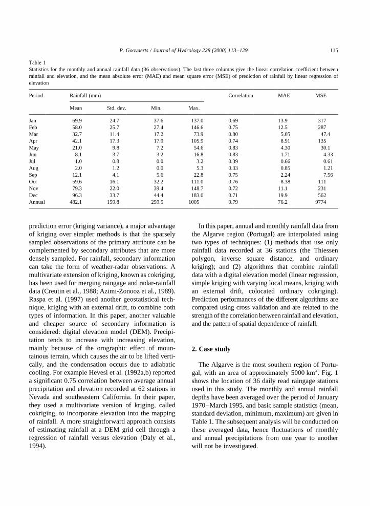
Table 1Statistics for the monthly and annual rainfall data (36 observations). The last three columns give the linear correlation coefficient betweenrainfall and elevation, and the mean absolute error (MAE) and mean square error (MSE) of prediction of rainfall by linear regression ofelevation

Period Rainfall (mm) Correlation MAE MSE

Mean Std. dev. Min. Max.

Jan 69.9 24.7 37.6 137.0 0.69 13.9 317Feb 58.0 25.7 27.4 146.6 0.75 12.5 287Mar 32.7 11.4 17.2 73.9 0.80 5.05 47.4Apr 42.1 17.3 17.9 105.9 0.74 8.91 135May 21.0 9.8 7.2 54.6 0.83 4.30 30.1Jun 8.1 3.7 3.2 16.8 0.83 1.71 4.33Jul 1.0 0.8 0.0 3.2 0.39 0.66 0.61Aug 2.0 1.2 0.0 5.3 0.33 0.85 1.21Sep 12.1 4.1 5.6 22.8 0.75 2.24 7.56Oct 59.6 16.1 32.2 111.0 0.76 8.38 111Nov 79.3 22.0 39.4 148.7 0.72 11.1 231Dec 96.3 33.7 44.4 183.0 0.71 19.9 562Annual 482.1 159.8 259.5 1005 0.79 76.2 9774

Another source of information is the elevation mapshown in Fig. 2. Each grid cell represents 1 km2 andits elevation was computed as the average of theelevations at 4 discrete points within the cell. Therelief is dominated by the two main Algarve’s moun-tains: the Monchique (left) and the Caldeira˜o (right).Table 1 indicates that the correlation between rainfalland elevation ranges from 0.33 to 0.83, hence it seemsworth accounting for this exhaustive secondary infor-mation into the mapping of rainfall. The control ofelevation on the spatial distribution of rainfallexplains the moderate to strong correlation betweenmonthly rainfall data, see Table 2. Apart from the twodry months of July and August the correlation rangesfrom 0.50 to 0.97. The correlation coefficients ofTable 2 have been averaged as a function of thetime lag between months, excluding July and August.Fig. 3 shows that the average correlation betweenrainfall measured over two consecutive months�lag�1� is 0.9 and slightly decreases to 0.8 as the separationtime increases.

3. Interpolation procedures

This section briefly introduces the different esti-mators used in the case study. Interested readersshould refer to Goovaerts (1997) for a detailed presen-tation of the different kriging algorithms, and Deutschand Journel (1998) for their implementation in thepublic-domain Geostatistical Software Library(Gslib).

3.1. Univariate estimation

Consider first the problem of estimating the rainfalldepthz at an unsampled locationu using only rainfalldata. Let {z�ua�;a � 1;…;n} be the set of rainfalldata measured atn� 36 locationsua .

The most straightforward approach is the Thiessen


Fig. 2. Digital elevation model.

Table 2Matrix of linear correlation coefficients between monthly rainfall data (36 observations)

Period Jan Feb Mar Apr May Jun Jul Aug Sep Oct Nov Dec

Jan 1.00 0.97 0.86 0.85 0.84 0.78 0.23 0.31 0.58 0.88 0.94 0.94Feb 1.00 0.92 0.91 0.87 0.81 0.22 0.42 0.64 0.92 0.96 0.93Mar 1.00 0.96 0.89 0.80 0.20 0.47 0.71 0.89 0.89 0.81Apr 1.00 0.91 0.82 0.20 0.42 0.71 0.91 0.89 0.78May 1.00 0.88 0.33 0.36 0.75 0.90 0.85 0.78Jun 1.00 0.38 0.34 0.77 0.84 0.79 0.72Jul 1.00 20.04 0.26 0.12 0.24 0.34Aug 1.00 0.46 0.37 0.35 0.31Sep 1.00 0.75 0.65 0.50Oct 1.00 0.89 0.81Nov 1.00 0.91Dec 1.00

Fig. 3. Average correlation between monthly rainfall data measuredat increasing time intervals: 1–5 months.

polygon method whereby the value of the closestobservation is simply assigned tou:

zpPol�u� � z�ua 0 � with uu 2 ua 0 u , uu 2 uau ;a ± a 0:

�1�

Fig. 4 (2nd graph) shows the map of annual rainfallinterpolated at the nodes of a 1× 1 km2 grid corre-sponding to the resolution of the elevation model. Themap displays the characteristic polygonal zones ofinfluence around the 36 gages.

To avoid unrealistic patchy maps, the depthzcan beestimated as a linear combination of several surround-ing observations, with the weights being inverselyproportional to the square distance between obser-vations andu:

zpInv�u� � 1Xn�u�

a�1

la�u�

Xn�u�a�1

la�u�z�ua�

with la�u� � 1

uu 2 uau2

�2�

Fig. 4 (3rd graph) shows the map of annual rainfallproduced using the inverse square distance methodandn�u� � 16 surrounding observations.

The basic idea behind the weighting scheme (2) isthat observations that are close to each other on theground tend to be more alike than those further apart,hence observations closer tou should receive a largerweight. Instead of the Euclidian distance, geostatisticsuses the semivariogram as a measure of dissimilaritybetween observations. The experimental semivario-gram g�h� is computed as half the average squareddifference between the components of data pairs:

g�h� � 12N�h�

XN�h�a�1

�z�ua�2 z�ua 1 h��2; �3�

whereN(h) is the number of pairs of data locations avector h apart. The semivariogram is a function ofboth the distance and direction, and so it can accountfor direction-dependent variability (anisotropic spatialpattern).

Fig. 5 (top graph) shows the semivariogram ofannual rainfall computed from the 36 data of Fig. 4.Because of the lack of data only the omnidirectionalsemivariogram was computed, and hence the spatialvariability is assumed to be identical in all directions.Semivariogram values increase with the separationdistance, reflecting our intuitive feeling that two rain-fall data close to each other on the ground are morealike, and thus their squared difference is smaller, thanthose that are further apart. The semivariogramreaches a maximum at 25 km before dipping and fluc-tuating around a sill value. The so-called “hole effect”typically reflects pseudo-periodic or cyclic phenom-ena (Journel and Huijbregts, 1978, p. 403). Here, the


Fig. 4. Annual rainfall maps obtained by interpolation of 36 obser-vations (top map) using the Thiessen polygon, inverse squaredistance, and ordinary kriging.

hole effect relates to the existence of two mountains40 km apart (recall Fig. 2) which creates two high-valued areas in the rainfall field.

Kriging is a generalized least-square regression

technique that allows one to account for the spatialdependence between observations, as revealed by thesemivariogram, into spatial prediction. Most of geos-tatistics is based on the concept of a random function,whereby the set of unknown values is regarded as a setof spatially dependent random variables. Eachmeasurementz�ua� is thus interpreted as a particularrealization of a random variableZ�ua�. Interestedreaders should refer to textbooks such as Isaaks andSrivastava (1989, pp. 196–236) or Goovaerts (1997,pp. 59–74) for a detailed presentation of the theory ofrandom functions. Like the inverse square distancemethod, geostatistical interpolation amounts at esti-mating the unknown rainfall depthzat the unsampledlocation u as a linear combination of neighboringobservations:

zpOK�u� �

Xn�u�a�1

lOKa �u�z�ua� with

Xn�u�a�1

lOKa �u� � 1: �4�

The ordinary kriging weightslOKa �u� are determined

such as to minimize the estimation variance,Var{Zp

OK�u�2 Z�u�} ; while ensuring the unbiased-ness of the estimator, E{Zp

OK�u�2 Z�u�} � 0: Theseweights are obtained by solving a system of linearequations which is known as “ordinary krigingsystem”:

Xn�u�b�1

lb�u�g �ua 2 ub�2 m�u� � g �ua 2 u� a � 1;…; n�u�

Xn�u�b�1

lb�u� � 1

8>>>>><>>>>>: �5�

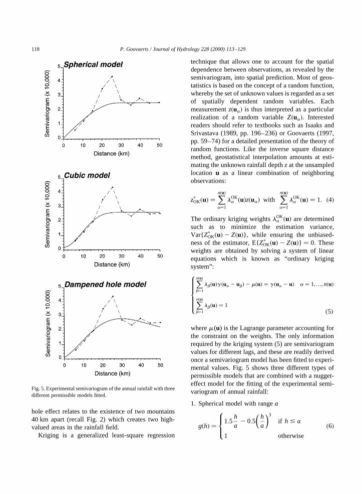
wherem (u) is the Lagrange parameter accounting forthe constraint on the weights. The only informationrequired by the kriging system (5) are semivariogramvalues for different lags, and these are readily derivedonce a semivariogram model has been fitted to experi-mental values. Fig. 5 shows three different types ofpermissible models that are combined with a nugget-effect model for the fitting of the experimental semi-variogram of annual rainfall:

1. Spherical model with rangea

g�h� � 1:5ha

2 0:5ha

� �3

if h # a

1 otherwise

8><>: �6�


Fig. 5. Experimental semivariogram of the annual rainfall with threedifferent permissible models fitted.

2. Cubic model with rangea

g�h��

7ha

� �2

28:75ha

� �3

13:5ha

� �5

20:75ha

� �7

if h # a

1 otherwise

8>>>>>><>>>>>>:�7�

3. Dampened hole effect model

g�h� � 1:0 2 exp23h

d

� �cos

hap

� ��8�

whered is the distance at which 95% of the holeeffect is dampened out.

The spherical model is the most widely used semi-variogram model and is characterized by a linearbehavior at the origin. The cubic model (Galli et al.,1984; Chiles and Delfiner, 1999, p. 84) displays aparabolic behavior at the origin and is preferred tothe Gaussian model because it avoids numericalunstability in kriging system (Wackernagel, 1998, p.120). Although no direct information is available onthe variability of rainfall over very short distances (thefirst semivariogram value corresponds to a lag of5.9 km), ancillary information, such as the moredetailed semivariogram of a correlated attribute likealtitude (Fig. 6), suggests that one can expect a para-bolic behavior for the first lags. Note that a very regu-

lar behavior near the origin can be combined with anugget effect, the latter reflecting measurement errorsthat are superimposed on the underlying continuousphenomenon. The last type of function is morecomplex and used to model hole effect (Deutsch andJournel, 1998, p. 26). The three models have beenfitted using regression and are such that the weightedsum of squares (WSS) of differences between experi-mentalg�hk� and modelg �hk� semivariogram valuesis minimum:

WSS�XKk�1

v�hk��g�hk�2 g �hk��2 �9�

The weights were taken asN�hk�=�g �hk��2 in orderto give more importance to the first lags and the onescomputed from more data pairs. The cubic model hasbeen retained because it yields the smallest WSSvalue while being more parsimonious (less parametersto estimate) than the dampened hole effect model. Fig.4 (bottom graph) shows the rainfall map produced byordinary kriging using the cubic semivariogrammodel and the 16 closest observations at each gridnode. Like the inverse square distance method, therainfall map is quite crude, which stresses theimportance of accounting for more denselysampled information, such as the digital elevationmodel of Fig. 2.

3.2. Accounting for elevation

Consider now the situation where the rainfall data{ z�ua�;a � 1;…;n} are supplemented by elevationdata available at all estimation grid nodes and denotedy(u).

A straightforward approach consists of predictingthe rainfall as a function of the co-located elevation,e.g. using a linear relation such as:

zp�u� � f � y�u�� ap0 1 ap

1y�u� �10�where the two regression coefficientsap

0;ap1 are esti-

mated from the set of collocated rainfall and elevationdata {�z�ua�; y�ua��; a � 1;…;n} : For example, therelation between annual rainfall and elevation wasmodeled as z�u� � 324:1 1 0:922y�u� R2 � 0:62;leading to the rainfall map shown at the top of Fig.7. A major shortcoming of this type of regression isthat the rainfall at a particular grid nodeu is derivedonly from the elevation atu, regardless of the records


Fig. 6. Experimental semivariogram of elevation computed from theDEM of Fig. 2.

at the surrounding raingagesua . Such an approachamounts at assuming that the residual valuesr�ua� �z�ua�2 f � y�ua�� are spatially uncorrelated. Spatialcorrelation of the residuals or of the rainfallobservations can be taken into account usingthe three types of geostatistical algorithmsdescribed below.

Simple kriging with varying local means (SKlm)amounts at replacing the known stationary mean inthe simple kriging estimate by known varying

means mpSK�u� derived from the secondary infor-

mation (Goovaerts, 1997, pp. 190–191):

zpSKlm�u�2 mp

SK�u� �Xn�u�a�1

lSKa �u��z�ua�2 mp

SK�ua��

�11�If the local means are derived using a relation of type(10), the SKlm estimate can be rewritten as the sum ofthe regression estimatef � y�u�� mp

SK�u� and the SKestimate of the residual value atu:

zpSKlm�u� � f � y�u��1

Xn�u�a�1

lSKa �u�r�ua� �12�

where the weightslSKa �u� are obtained by solving the

simple kriging system:Xn�u�b�1

lSKb �u�CR�ua 2 ub� � CR�ua 2 u�

a � 1;…;n�u� (13)

whereCR(h) is the covariance function of the residualRF R�u� � Z�u�2 m�u�; not that ofZ(u) itself. If theresiduals are uncorrelated,CR�h� � 0;h; hence allkriging weights in Eq. (12) are zero and the SKlmestimate is but the value provided by linear regression.Unlike the ordinary kriging system (5), the SK system(13) can be expressed in terms of only covariancesbecause of the lack of constraints on kriging weights(Goovaerts, 1997, p. 135). However, the commonpractice consists of estimating and modeling thesemivariogramgR�h�, then retrieving the covarianceCR�h� asCR�0�2 gR�h�: This conversion from semi-variogram to covariance values is automaticallyperformed within most geostatistical softwares,hence the user typically provides only the semivario-gram model. For example Fig. 8 shows the semi-variogram of residuals for annual rainfall with themodel fitted. This model was used to generate therainfall map in Fig. 7 (2nd graph). The impact ofelevation on the rainfall map is less pronouncedthan for the map generated using linear regressionthat was but a rescaling of the elevation model (Fig.7, top graph).

Like the SKlm approach, kriging with an externaldrift (KED) uses the secondary information to derivethe local mean of the primary attributez, then


Fig. 7. Annual rainfall maps obtained by interpolation of 36 obser-vations accounting for the digital elevation model of Fig. 2. Fouralgorithms are considered: linear regression, simple kriging withvarying local means, kriging with an external drift and colocatedordinary cokriging.

performs simple kriging on the corresponding resi-duals:

zpKED�u�2 mp

KED�u� �Xn�u�a�1

lSKa �u��z�ua�2 mp

KED�ua��

�14�

where mpKED�u� � ap

0�u�1 ap1�u�y�u�: Estimates (11)

and (15) differ by the definition of the local mean ortrend. The trend coefficientsap

0 and ap1 are derived

once and independently of the kriging system in theSKlm approach, whereas in the KED approach theregression coefficientsap

0�u� andap1�u� are implicitly

estimated through the kriging system within eachsearch neighborhood. In other words, the relationbetween elevation and rainfall is assessed locally,which allows one to account for changes in correlationacross the study area. The coefficientsap

0�u� andap1�u�

can be computed and mapped for interpretationpurposes (e.g. see Goovaerts, 1997, p. 201) but theyare not required for estimation. Indeed, the usual andequivalent expression for the KED estimate(Wackernagel, 1998, pp. 199–201; Goovaerts, 1997,pp. 194–198) is:

zpKED�u� �

Xn�u�a�1

lKEDa �u�z�ua� �15�

The kriging weightslKEDa �u� are the solution

of the following system of �n�u�1 2� linear

equations:

Xn�u�b�1

lKEDb �u�gR�ua 2 ub�1 mKED

0 �u�

1mKED1 �u�y�ua� � gR�ua 2 u� a � 1;…;n�u�Xn�u�

b�1

lKEDb �u� � 1

Xn�u�b�1

lKEDb �u�y�ub� � y�u�

8>>>>>>>>>>>>>><>>>>>>>>>>>>>>: �16�

wheremKED0 �u� and mKED

1 �u� are 2 Lagrange para-meters accounting for the constraints on theweights. Note that elevation datay(ua ) and y(u)intervene in the kriging system but they are notdirectly included in the estimate (15). Fig. 7 (thirdgraph) shows the map of KED estimates of annualrainfall, which looks very similar to the SKlmmap.

Another approach for incorporating secondaryinformation is cokriging, a multivariate extension ofkriging (Goovaerts, 1997, pp. 203–248). When thesecondary variable is known everywhere and variessmoothly across the study area (e.g. elevation) there islittle loss in retaining in the cokriging system only thesecondary datum co-located with the locationu beingestimated (Xu et al., 1992; Goovaerts, 1998). Indeedthe co-located elevationy(u) tends to screen the influ-ence of further away elevation data. Moreover, usingmultiple secondary data can lead to unstable cokrigingsystems because the correlation between close eleva-tion data is much greater than the correlation betweendistant rainfall data (Goovaerts, 1997, p. 235). The“co-located” cokriging estimate is then:

zpCK�u� �

Xn�u�a�1

lCKa �u�z�ua�1 lCK�u�� y�u�2 mY 1 mZ�;

�17�wheremZ andmY are the global means of the rainfalland elevation data, see Table 1. The second term ofEq. (17) corresponds to a rescaling of the secondaryvariable (elevation) to the mean of the primary vari-able (rainfall) to ensure unbiased estimation. Themain difference between cokriging and the twoprevious geostatistical algorithms lies in how the


Fig. 8. Experimental residual semivariogram of annual rainfall withthe model fitted.

elevation value is handled. Whereas that datumdirectly influences the cokriging estimate, in theSKlm and KED approaches elevation provides infor-mation only about the primary trend at locationu. Thecokriging weights are solutions of the following

system of�n�u�1 2� linear equations:

Xn�u�b�1

lCKb �u�gZZ�ua 2 ub�1 lCK�u�gZY�ua 2 u�

1mCK�u� � gZZ�ua 2 u� a � 1;…; n�u�Xn�u�b�1

lCKb �u�gYZ�u 2 ub�1 lCK�u�gYY�0�

1mCK�u� � gZY�0�Xn�u�b�1

lCKb �u�1 lCK�u� � 1

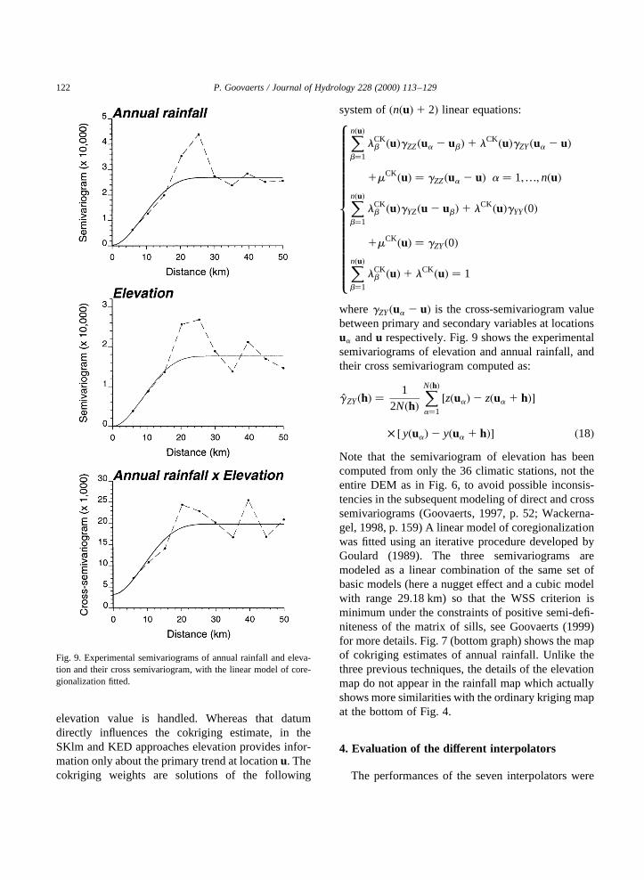
8>>>>>>>>>>>>>>>>><>>>>>>>>>>>>>>>>>:wheregZY�ua 2 u� is the cross-semivariogram valuebetween primary and secondary variables at locationsua andu respectively. Fig. 9 shows the experimentalsemivariograms of elevation and annual rainfall, andtheir cross semivariogram computed as:

gZY�h� � 12N�h�

XN�h�a�1

�z�ua�2 z�ua 1 h��

� � y�ua�2 y�ua 1 h�� 18�Note that the semivariogram of elevation has beencomputed from only the 36 climatic stations, not theentire DEM as in Fig. 6, to avoid possible inconsis-tencies in the subsequent modeling of direct and crosssemivariograms (Goovaerts, 1997, p. 52; Wackerna-gel, 1998, p. 159) A linear model of coregionalizationwas fitted using an iterative procedure developed byGoulard (1989). The three semivariograms aremodeled as a linear combination of the same set ofbasic models (here a nugget effect and a cubic modelwith range 29.18 km) so that the WSS criterion isminimum under the constraints of positive semi-defi-niteness of the matrix of sills, see Goovaerts (1999)for more details. Fig. 7 (bottom graph) shows the mapof cokriging estimates of annual rainfall. Unlike thethree previous techniques, the details of the elevationmap do not appear in the rainfall map which actuallyshows more similarities with the ordinary kriging mapat the bottom of Fig. 4.

4. Evaluation of the different interpolators

The performances of the seven interpolators were


Fig. 9. Experimental semivariograms of annual rainfall and eleva-tion and their cross semivariogram, with the linear model of core-gionalization fitted.

assessed and compared using cross validation (Isaaksand Srivastava, 1989, pp. 351–368). The idea consistsof removing temporarily one rainfall observation at atime from the data set and “re-estimate” this valuefrom remaining data using the alternative algorithms.The comparison criterion is the mean square error(MSE) of prediction which measures the averagesquare difference between the true rainfallz(ua) andits estimatezp(ua ):

MSE� 1n

Xna�1

�z�ua�2 zp�ua��2 �19�

wheren� 36 for the Algarve data set. The value ofthis criterion should be close to zero if the algorithm isaccurate. For linear regression, the MSE was simplycomputed as the average square residual value for thelinear model fitted using all 36 observations, whichmeans that the prediction error would tend to beunderestimated for this method. Although the variouskriging interpolators provide an estimate of the errorvariance, the latter has not been retained as a perfor-mance criterion because in practice it usually provideslittle information on the reliability of the kriging esti-mate, as reminded by several authors (Journel, 1993;Armstrong, 1994).

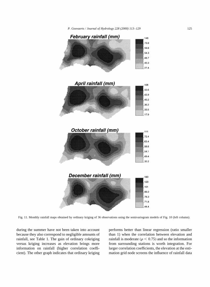
The same interpolators as described in previoussections and illustrated for annual rainfall have beenapplied to monthly rainfall data. Fig. 10 shows, forexample, the semivariograms of raw rainfall data andresiduals for four of the wettest months (recall Table1). Because of the control of the relief on the spatialdistribution of precipitations, the semivariogramshave similar shape although the nugget effect andrange of the cubic model fluctuate from one monthto another. For the same four months, Fig. 11 showsthe maps of ordinary kriging estimates; to facilitatethe comparison of grayscale maps, six equally prob-able classes of values have been created for eachmonth. Despite the similarity of their semivariograms,monthly rainfall maps show slightly different patterns:smaller precipitations are recorded along the WestCoast in December and February whereas high preci-pitation cells move towards the West in April andOctober.

Fig. 12 shows the mean square errors of predictionproduced by each of the seven interpolation algo-rithms for the monthly (Jan–Dec) and annual (Ann)

rainfall. Results are expressed as proportions of theprediction error of the linear regression approach,hence absolute values are easily retrieved by multi-plying these percentages by the values of Table 1 (lastcolumn). The conclusions are as follows:

1. Larger predictions errors are obtained for the threealgorithms that ignore elevation, with the worstresults produced by Thiessen polygon. It is note-worthy that for several months, and on averageover the year, ordinary kriging yields smallerprediction errors than linear regression of rainfallagainst elevation.

2. Except for the period from June to Septemberwhich is characterized by low rainfall amounts(Table 1), multivariate geostatistical algorithmsperform better than linear regression which disre-gards the information provided by surroundingclimatic stations.

3. Among geostatistical algorithms that account forelevation, simple kriging with varying localmeans and kriging with an external drift yieldslightly better results than the more complex ordin-ary cokriging.

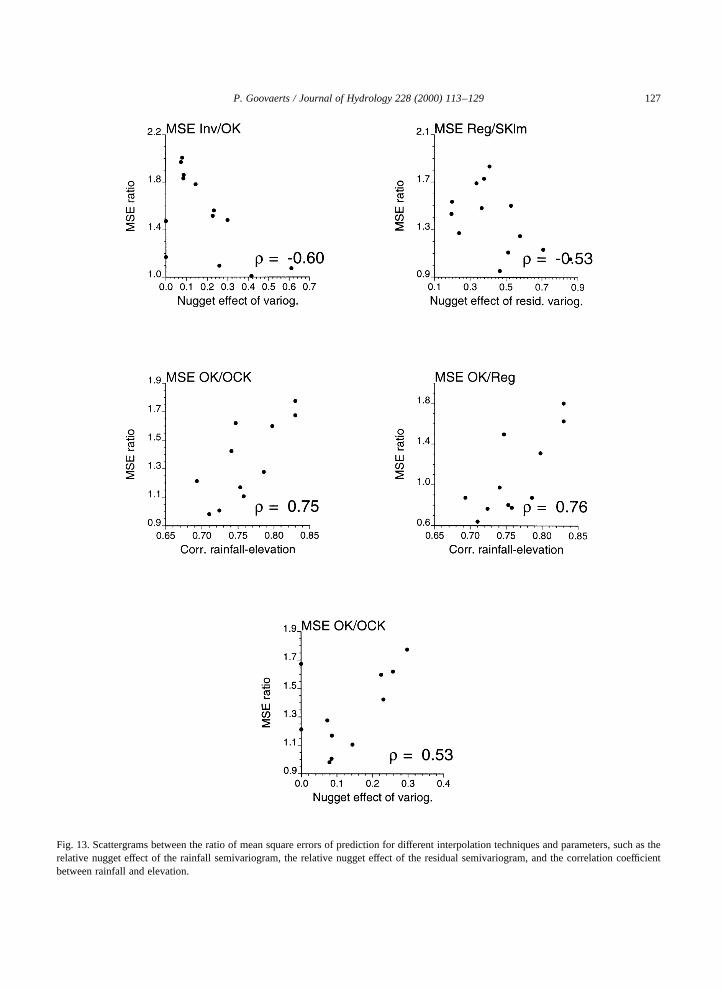
To identify the factors that might be responsible forthese relative prediction performances, ratios of MSEvalues have been plotted against parameters, such asthe relative nugget effect of the rainfall semivario-gram, the relative nugget effect of the residual semi-variogram, and the correlation coefficient betweenrainfall and elevation. The first scattergram (Fig. 13,left top graph) shows that the benefit of using ordinarykriging instead of the inverse square distance method(i.e. a larger MSE ratio Inv/OK) decreases as thespatial dependence between observations weakens,which is indicated by a larger relative nugget effectfor the rainfall semivariogram. Similarly, the benefitof using a geostatistical approach (SKlm) instead oflinear regression to account for elevation decreases asthe spatial dependence between residual data weakens(larger nugget effect for the residual semivariogram),see Fig. 13 (right top graph).

The two middle graphs of Fig. 13 show the impactof the strength of the correlation between elevationand rainfall on the relative performances of ordinarykriging versus cokriging (left graph) and ordinarykriging versus linear regression (right graph). Notethat the smallest correlation coefficients observed



Fig. 10. Experimental semivariograms of monthly rainfall before and after substraction of the local means provided by linear regression ofrainfall against elevation at the 36 climatic stations, with the model fitted using weighted least-square regression.

during the summer have not been taken into accountbecause they also correspond to negligible amounts ofrainfall, see Table 1. The gain of ordinary cokrigingversus kriging increases as elevation brings moreinformation on rainfall (higher correlation coeffi-cient). The other graph indicates that ordinary kriging

performs better than linear regression (ratio smallerthan 1) when the correlation between elevation andrainfall is moderate�r , 0:75� and so the informationfrom surrounding stations is worth integration. Forlarger correlation coefficients, the elevation at the esti-mation grid node screens the influence of rainfall data


Fig. 11. Monthly rainfall maps obtained by ordinary kriging of 36 observations using the semivariogram models of Fig. 10 (left column).

at surrounding sites and so spatial information is lessvaluable.

Goovaerts (1997, pp. 217–221), showed that thecontribution of the secondary information to thecokriging estimate depends not only on the correlationbetween primary and secondary variables, but also ontheir patterns of spatial continuity. As the relativenugget effect of the primary semivariogram increases,the increasingly noisy primary data carry less infor-mation and the secondary data have larger weight, inparticular when the cross semivariogram and thesemivariogram of the secondary variable have asmall relative nugget effect. As the semivariogramof elevation has typically a small nugget effect (recallFig. 6), one can expect similar results, as confirmed bythe bottom graph of Fig. 13. The gain of ordinarycokriging versus kriging increases as the spatialdependence between observations weakens, which isindicated by a larger relative nugget effect for therainfall semivariogram (as for the middle graphsJuly and August results are not included).

5. Conclusions

Our results confirm previous findings (e.g. Creutinand Obled, 1982) that for low-density networks ofraingages geostatistical interpolation outperformstechniques, such as the inverse square distance orThiessen polygon, that ignore the pattern of spatialdependence which is usually observed for rainfalldata: the mean square error of kriging prediction isup to half the error produced using inverse squaredistance. Prediction can be further improved if corre-lated secondary information, such as a digital eleva-tion model, is taken into account. This paper hasreviewed different ways to incorporate such exhaus-tive secondary information, and cross validation hasshown that prediction performances can vary greatlyamong algorithms.

The most straightforward approach consists ofderiving the rainfall value directly from the colocatedelevation through a (non)linear regression. By sodoing, one ignores however the information provided


Fig. 12. Mean square error of prediction produced by each of the seven interpolation algorithms for monthly (Jan–Dec) and annual (Ann)rainfall. Results are expressed as proportions of the prediction error of the linear regression approach.


Fig. 13. Scattergrams between the ratio of mean square errors of prediction for different interpolation techniques and parameters, such as therelative nugget effect of the rainfall semivariogram, the relative nugget effect of the residual semivariogram, and the correlation coefficientbetween rainfall and elevation.

by surrounding climatic stations which is criticalwhen the correlation between the two variables isnot too strong and when the residuals are spatiallycorrelated. In this case study, ordinary kriging whichignores elevation is in fact better than linear regres-sion when the correlation is smaller than 0.75! Aneasy way to account for both elevation and spatialcorrelation is to interpolate the regression residualsusing geostatistics, that is to use simple kriging withvarying local means (SKlm). For most months SKlmprovides the smallest mean square error of predictionand so performs better that the more sophisticatedkriging with an external drift (KED) that evaluatesthe correlation between elevation and rainfall withineach search neighborhood. The last technique is cokri-ging that interpolates the rainfall as a linear combina-tion of surrounding rainfall observations and thecolocated elevation. This approach is the mostdemanding because three semivariograms must beinferred and jointly modeled, a task that is howeveralleviated by the recent development of automaticfitting procedures. Cokriged maps show less detailsthan the SKlm and KED maps that are greatly influ-enced by the pattern of the DEM. In this case study,the additional complexity of cokriging does not payoff in that the prediction errors are not smaller than theones provided by SKlm and KED.

Further research should investigate whether otherenvironmental descriptors, such as the distance to thesea or the slope orientation, allow one to explain alarger proportion of the spatial variability displayedby rainfall. Whereas cokriging and kriging with multi-ple external drifts may become very cumbersome toapply, SKlm provides an easy way to incorporateseveral secondary variables and, for this data set, ityields the best prediction. In this case study, account-ing for elevation using multivariate geostatisticalalgorithms (SKlm, KED and OCK) generally reducesthe OK prediction error as long as the correlationcoefficient is larger than 0.75. A similar correlationthreshold has been reported by Asli and Marcotte(1995) who further concluded that the introductionof secondary information in estimation seems worthyonly for correlations above 0.4. The benefit of multi-variate techniques can therefore become marginal ifthe correlation between rainfall and elevation (orother environmental descriptors) is too small, as itmight be the case for rainfall accumulations during

shorter time steps. Besides the correlation betweenelevation and rainfall it is also important to look attheir patterns of spatial continuity. Elevation data thatare moderately correlated with rainfall (i.e. a correla-tion between 0.4 and 0.7) but exhibit a much smallerrelative nugget effect than the rainfall semivariogrammay still improve prediction using cokriging, in parti-cular if the nugget effect of the cross semivariogrambetween rainfall and elevation is small.

Acknowledgements

The author thanks Mr. Nuno de Santos Loureiro forthe Algarve data set.

References

Armstrong, M., 1994. Is research in mining geostats as dead as adodo? In: Dimitrakopoulos, R. (Ed.)., Geostatistics for The NextCentury, Kluwer Academic, Dordrecht, pp. 303–312.

Asli, M., Marcotte, D., 1995. Comparison of approaches to spatialestimation in a bivariate context. Math. Geol. 27 (5), 641–658.

Azimi-Zonooz, A., Krajewski, W.F., Bowles, D.S., Seo, D.J., 1989.Spatial rainfall estimation by linear and non-linear cokriging ofradar-rainfall and raingage data. Stochastic Hydrol. Hydraul. 3,51–67.

Bedient, P.B., Huber, W.C., 1992. Hydrology and FloodplainAnalysis. 2nd ed, Addison-Wesley, Reading, MA.

Borga, M., Vizzaccaro, A., 1997. On the interpolation of hydrologicvariables: formal equivalence of multiquadratic surface fittingand kriging. J. Hydrol. 195 (1–4), 160–171.

Chiles, J.-P., Delfiner, P., 1999. Geostatistics. Modeling SpatialUncertainty. Wiley, New York.

Creutin, J.D., Obled, C., 1982. Objective analyses and mappingtechniques for rainfall fields: an objective comparison. WaterResour. Res. 18 (2), 413–431.

Creutin, J.D., Delrieu, G., Lebel, T., 1988. Rain measurement byraingage-radar combination: a geostatistical approach. J. Atm.Oceanic Tech. 5 (1), 102–115.

Daly, C., Neilson, R.P., Phillips, D.L., 1994. A statistical topo-graphic model for mapping climatological precipitation overmontainous terrain. J. Appl. Meteor. 33 (2), 140–158.

Deutsch, C.V., Journel, A.G., 1998. GSLIB: Geostatistical SoftwareLibrary and User’s Guide. 2nd ed, Oxford University Press,New York.

Dirks, K.N., Hay, J.E., Stow, C.D., Harris, D., 1998. High-resolu-tion studies of rainfall on Norfolk Island Part II: interpolation ofrainfall data. J. Hydrol. 208 (3-4), 187–193.

Galli, A., Gerdil-Neuillet, F., Dadou, C., 1984. Factorial kriginganalysis: a substitute to spectral analysis of magnetic data. In:Verly, G., David, M., Journel, A.G., Mare´chal, A. (Eds.), Geo-statistics for Natural Resources Characterization, Reidel,Dordrecht, pp. 543–557.


Goovaerts, P., 1997. Geostatistics for Natural Resources Evalua-tion. Oxford University Press, New York.

Goovaerts, P., 1998. Ordinary cokriging revisited. Math. Geol. 30(1), 21–42.

Goovaerts, P., 1999. Geostatistics in soil science: state-of-the-artand perspectives. Geoderma 89, 1–46.

Goulard, M., 1989. Inference in a coregionalization model. In:Armstrong, M. (Ed.), Geostatistics, Kluwer Academic,Dordrecht, pp. 397–408.

Hevesi, J.A., Flint, A.L., Istok, J.D., 1992a. Precipitation estimationin mountainous terrain using multivariate geostatistics. Part I:structural analysis. J. Appl. Meteor. 31, 661–676.

Hevesi, J.A., Flint, A.L., Istok, J.D., 1992b. Precipitation estimationin mountainous terrain using multivariate geostatistics. Part II:Isohyetal maps. J. Appl. Meteor. 31, 677–688.

Isaaks, E.H., Srivastava, R.M., 1989. An Introduction to AppliedGeostatistics. Oxford University Press, New York.

Journel, A.G., 1993. Geostatistics: roadblocks and challenges. In:Soares, A. (Ed.), Geostatistics Tro´ia ‘92, Kluwer Academic,Dordrecht, pp. 213–224.

Journel, A.G., Huijbregts, C.J., 1978. Mining Geostatistics.Academic Press, New York.

McCuen, R.H., 1998. Hydrologic Analysis and Design. 2nd ed,Prentice Hall, Englewood Cliffs, NJ.

Phillips, D.L., Dolph, J., Marks, D., 1992. A comparison of geos-tatistical procedures for spatial analysis of precipitations inmountainous terrain. Agr. Forest Meteor. 58, 119–141.

Raspa, G., Tucci, M., Bruno, R., 1997. Reconstruction of rainfallfields by combining ground raingauges data with radar mapsusing external drift method. In: Baafi, E.Y., Schofield, N.A.(Eds.), Geostatistics Wollongong ’96, Kluwer Academic,Dordrecht, pp. 941–950.

Tabios, G.Q., Salas, J.D., 1985. A comparative analysis of techni-ques for spatial interpolation of precipitation. Water Resour.Bull. 21 (3), 365–380.

Thiessen, A.H., 1911. Precipitation averages for large areas.Monthly Weather Rev. 39 (7), 1082–1084.

Wackernagel, H., 1998. (completely revised). Multivariate Geosta-tistics. 2nd ed, Springer, Berlin.

Xu, W., Tran, T.T., Srivastava, R.M., Journel, A.G., 1992. Integrat-ing seismic data in reservoir modeling: the collocated cokrigingalternative. Society of Petroleum Engineers, paper no. 24742.


geostatistical approaches for incorporating elevation into ...geostatistical approaches for...

Documents