geotechnical earthquake engineering - nptelnptel.ac.in/courses/105101134/downloads/lec-20.pdf6 for...
TRANSCRIPT
Geotechnical Earthquake
Engineering
by
Dr. Deepankar Choudhury Humboldt Fellow, JSPS Fellow, BOYSCAST Fellow
Professor
Department of Civil Engineering
IIT Bombay, Powai, Mumbai 400 076, India.
Email: [email protected]
URL: http://www.civil.iitb.ac.in/~dc/
Lecture – 20

IIT Bombay, DC 2
Module – 5
Wave Propagation

6
For isotropic material, the coefficients must be independent of direction
Hooke’s law for an isotropic, linear, elastic material allows all
components of stress and strain to be expressed in terms of two Lame’s
constants. λ and µ.
12 21 13 31 23 32
44 55 66
11 22 33 2
c c c c c c
c c c
c c c
2
2
2
xx xx
yy yy
zz zz
xy xy
yz yz
zx zx
xx yy zz
The volumetric strain:
IIT Bombay, DC
Reference : Kramer (1996)

IIT Bombay, DC 7
Common Expressions for
Various Modulus
3 2
2
3
2
E
K
G
All components of stress and strain for an isotropic,
linear, elastic material follows Hooke’s law and can be
expressed in terms of two Lame’s constants, λ and µ.
Young’s modulus,
Bulk modulus,
Shear modulus,
Poisson’s ratio,
8
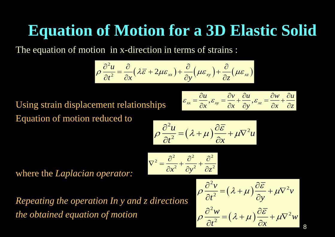
The equation of motion in x-direction in terms of strains :
Using strain displacement relationships
Equation of motion reduced to
where the Laplacian operator:
Repeating the operation In y and z directions
the obtained equation of motion
2
22 xx xy xz
u
t x y z
2
2
2
uu
t x
2 2 22
2 2 2x y z
, ,xx xy xz
u v u w u
x x y x z
22
2
22
2
vv
t y
ww
t x
Equation of Motion for a 3D Elastic Solid

IIT Bombay, DC 9 Reference : Kramer (1996)

IIT Bombay, DC 10
Solution of 3D Equation of Motion
The solution for the first type of wave can be calculated by differentiating each equations w.r.t. x, y and z and adding them together,
Rearranging, the wave equation is given by,
2
2 2
2t
2
2
2 2
t2
pv
2 2
1 2p
Gv
2 22 22 22 2 2
2 2 2 2 2 2 2 2 2
yy yyxx xxzz zz
t t t x y z x y z
Reference : Kramer (1996)

11
Solution of 3D Equation of Motion
The solution of second type of wave can be written in the 2 forms,
2
2
2
xx
t
2 2
1 2
p
s
v
v
A distortional (s) wave propagates through the solid at velocity
Comparing the velocities vp and vs,
s
Gv
2
2
w v w v
t y z y z
Reference : Kramer (1996)
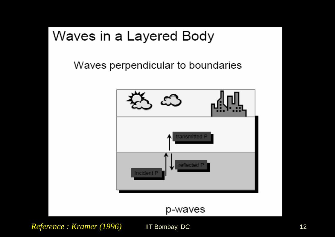
IIT Bombay, DC 12 Reference : Kramer (1996)

IIT Bombay, DC 13
Reference : Kramer (1996)

IIT Bombay, DC 14 Reference : Kramer (1996)

IIT Bombay, DC 15 Reference : Kramer (1996)

IIT Bombay, DC 16 Reference : Kramer (1996)

IIT Bombay, DC 17 Reference : Kramer (1996)

IIT Bombay, DC 18 Reference : Kramer (1996)
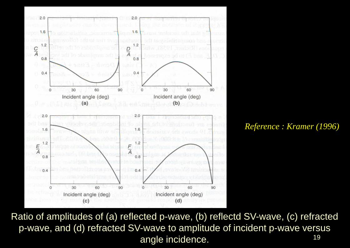
19
Ratio of amplitudes of (a) reflected p-wave, (b) reflectd SV-wave, (c) refracted
p-wave, and (d) refracted SV-wave to amplitude of incident p-wave versus
angle incidence.
Reference : Kramer (1996)

20
Ratio of amplitudes of (a) reflected p-wave, (b) reflected SV-wave, (c)
refracted p-wave, and (d) refracted SV-wave to amplitude of incident SV-wave
versus angle of incident.
Reference : Kramer (1996)

IIT Bombay, DC 21

22
Waves in Semi-Infinite Body
Motion induced by a typical plane wave that propagates in x-direction.
Wave motion does not vary in the y-direction.
Rayleigh wave
Reference : Kramer (1996)

23
Waves in a semi-infinite body
Two potential functions Φ and Ψ can be defined to describe the displacements
in the x and z directions:
The volumetric strain or dilation of the wave is given by
The rotation in x-z plane is given by
............... 5.1
............... 5.1
u ax z
w bz x
xx zz
2 22
2 2
u w
x z x x z z z x x z
2 22
2 22 y
u w
z x z x z z z x z x
Rayleigh waves
Reference : Kramer (1996)

24
Substituting the expressions for u and w into the equations of motions gives.
Solving the above equations simultaneously for shows.
2 22 2
2 2
2 22 2
2 2
2
2
x t z t x z
z t x t z x
2 2
2 2and
t t
22 2 2
2
22 2 2
2
2p
p
vt
vt
Reference : Kramer (1996)
Waves in Semi-Infinite Body

25
For harmonic wave with frequency ω and wave number kR, Rayleigh
wave velocity vR = ω/ kR, the potential function is expressed as
substituting these in the above equations.
........................... 5.2
.......................... 5.2
R
R
i t k x
i t k x
F z e a
G z e b
222
2 2
222
2 2
R
p
R
s
d F zF z k F z
v dz
d G zG z k G z
v dz
IIT Bombay, DC
Reference : Kramer (1996)
Waves in Semi-Infinite Body
26
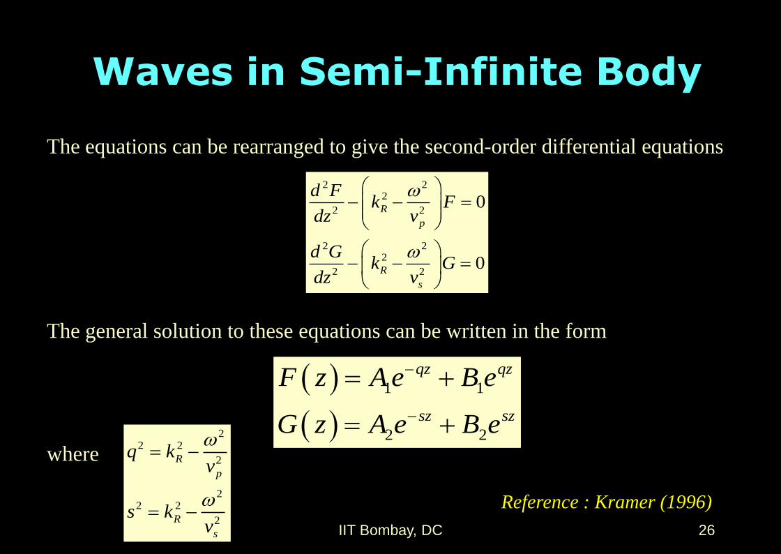
The equations can be rearranged to give the second-order differential equations
The general solution to these equations can be written in the form
where
2 22
2 2
2 22
2 2
0
0
R
p
R
s
d Fk F
dz v
d Gk G
dz v
1 1
2 2
qz qz
sz sz
F z A e B e
G z A e B e
22 2
2
22 2
2
R
p
R
s
q kv
s kv
IIT Bombay, DC
Reference : Kramer (1996)
Waves in Semi-Infinite Body

27
The potential function can be written as
Since neither shear nor normal stresses can exist at the free surface of the half-
space , when z = 0, therefore
1
2
R
R
qz i t k x
sz i t k x
A e
A e
0xz zz
2 2 0
0
zz zz
xz xz
dw
dz
dw du
dx dz
IIT Bombay, DC
Reference : Kramer (1996)
Waves in Semi-Infinite Body
28
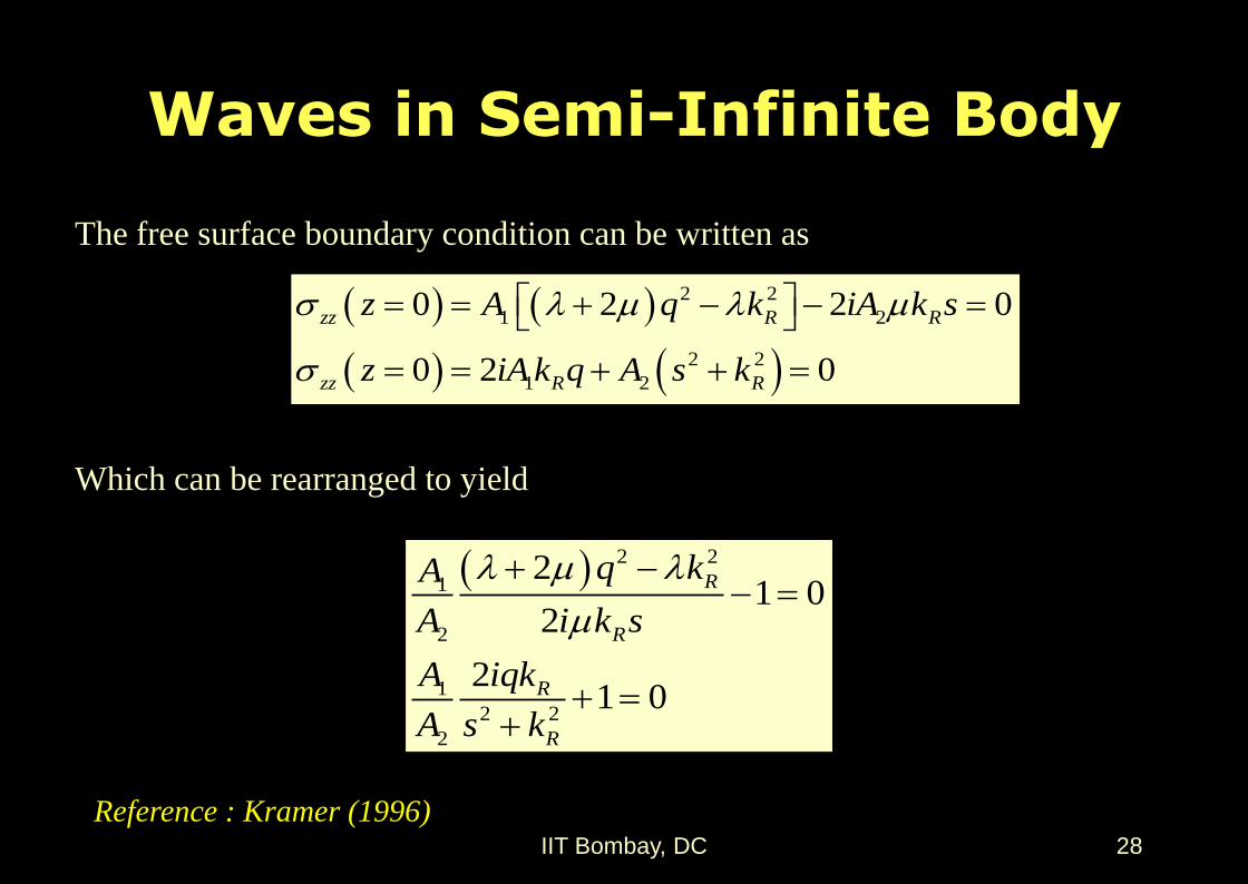
The free surface boundary condition can be written as
Which can be rearranged to yield
2 2
1 2
2 2
1 2
0 2 2 0
0 2 0
zz R R
zz R R
z A q k iA k s
z iA k q A s k
2 2
1
2
1
2 2
2
21 0
2
21 0
R
R
R
R
q kA
A i k s
A iqk
A s k
IIT Bombay, DC
Reference : Kramer (1996)
Waves in Semi-Infinite Body
29
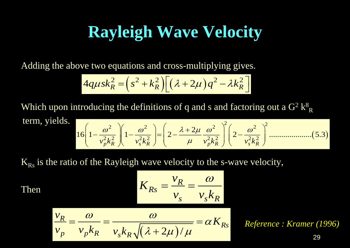
Rayleigh Wave Velocity
Adding the above two equations and cross-multiplying gives.
Which upon introducing the definitions of q and s and factoring out a G2 k8R
term, yields.
KRs is the ratio of the Rayleigh wave velocity to the s-wave velocity,
Then
2 2 2 2 24 2R R Rq sk s k q k
2 22 2 2 2
2 2 2 2 2 2 2 2
216 1 1 2 2 ..................... 5.3
p R s R p R s Rv k v k v k v k
RRs
s s R
vK
v v k
2 /
RRs
p p R s R
vK
v v k v k
Reference : Kramer (1996)

30
/ 2 1 2 / 2 2
Hence previous equation can be rewritten as
2
22 2 2 2 2 2
2
116 1 1 2 2Rs Rs Rs RsK K K K
Which can be rearranged to the equation
6 4 2 2 28 24 16 16 1 0Rs Rs RsK K K
IIT Bombay, DC Reference : Kramer (1996)
Rayleigh Wave Velocity
31
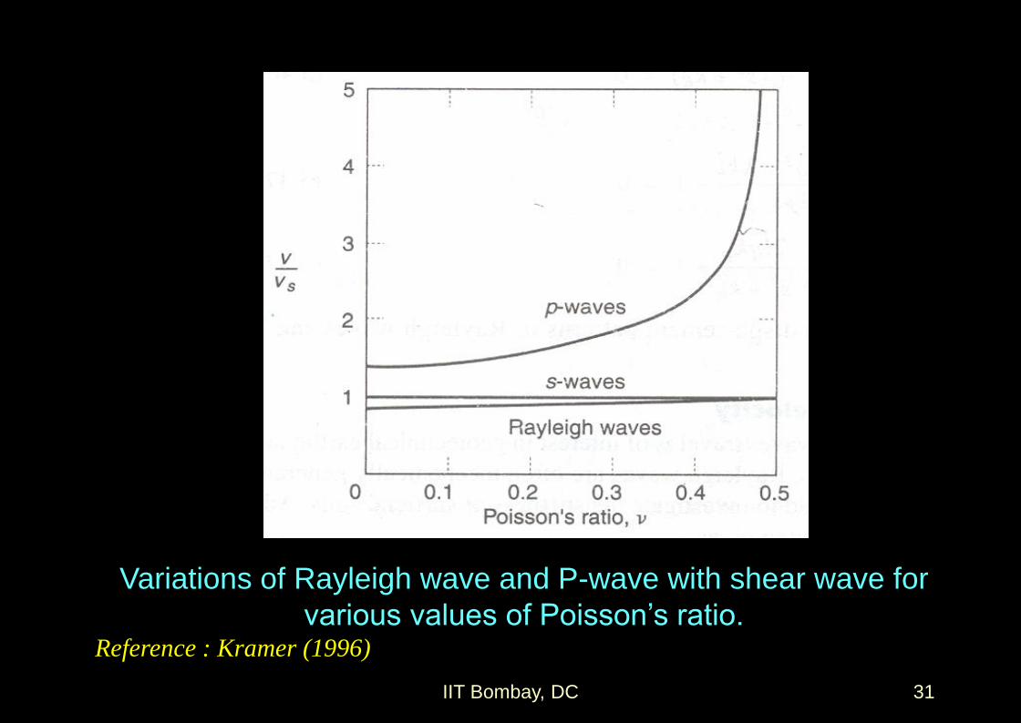
Variations of Rayleigh wave and P-wave with shear wave for
various values of Poisson’s ratio.
IIT Bombay, DC
Reference : Kramer (1996)

IIT Bombay, DC 32 Reference : Kramer (1996)

IIT Bombay, DC 33
Love Wave
Typical condition for generation of Love Wave
for softer surficial layer (G1/1 < G2/2)
overlaying elastic half-space
Reference : Kramer (1996)
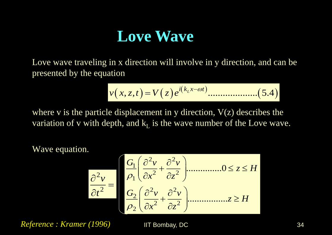
34
Love wave traveling in x direction will involve in y direction, and can be
presented by the equation
where v is the particle displacement in y direction, V(z) describes the
variation of v with depth, and kL is the wave number of the Love wave.
Wave equation.
, , .................... 5.4Li k x tv x z t V z e
2
2
v
t
2 21
2 21
2 22
2 22
...............0
.................
G v vz H
x z
G v vz H
x z
IIT Bombay, DC Reference : Kramer (1996)
Love Wave

35
The amplitude can be shown vary with depth
where A and B coefficients describe the amplitude of down going and up
going waves, respectively, and
Since the half space extends to infinite depth, B2 = 0, the requirement that all
stresses vanish at the ground surface is satisfied if
V z
1 1
2 2
1 1
2 2
......................0
.....................
v z v z
v z v z
A e B e z H
A e B e z H
2 2
11 1/
Lkv
G
2 2
22 2/
Lkv
G
1 1 1 1
1 1 1 1 1 1 1 0Li k x t v z v z v z v zV zve A v e v B e A B v e e
z z
Reference : Kramer (1996)
Love Wave

36
The love wave velocity can be
obtained by:
1/ 2 2 222
2 211
2 21
1 1
1 1tan
1 1
L s
s L
s L
v vGH
Gv v
v v
Variation of Love wave velocity with frequency.
IIT Bombay, DC
Reference : Kramer (1996)
Love Wave

IIT Bombay, DC 37
Variation of particle displacement amplitude with depth for
Love wave
Reference : Kramer (1996)

38
Three-Dimensional Case: Inclined Wave
Ray path, ray, and wavefront for (a) plane wave and (b) curved wavefront.
sinconsant
i
v
IIT Bombay, DC
Reference : Kramer (1996)

39
Reflected and refracted rays resulting from incident (a) p-wave,
(b) SV- wave, and (c) SH-wave.
IIT Bombay, DC
Reference : Kramer (1996)

40
Refraction of an SH-wave ray path through series of successively softer
(lower vs) layers. Note that orientation f ray path becomes closer to
vertical as ground surface is approached. Reflected rays are not shown.
IIT Bombay, DC
Reference : Kramer (1996)

IIT Bombay, DC 41

IIT Bombay, DC 42
IIT Bombay, DC 43

IIT Bombay, DC 44
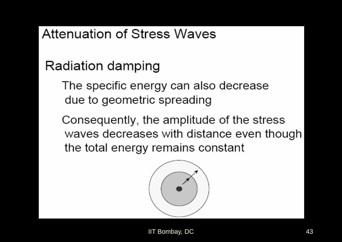
Attenuation of Stress Waves
Both types of damping are important,
though one may dominate the other in
specific situations
IIT Bombay, DC 45
Case Studies
IIT Bombay, DC 46
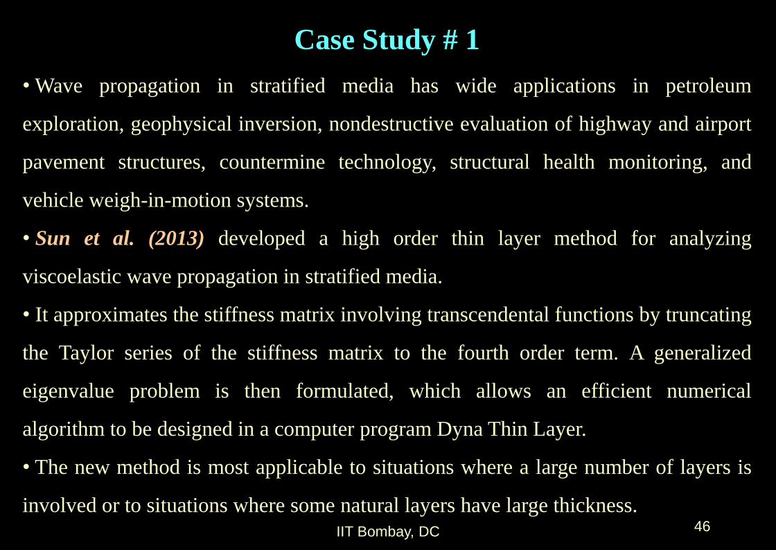
Case Study # 1
• Wave propagation in stratified media has wide applications in petroleum
exploration, geophysical inversion, nondestructive evaluation of highway and airport
pavement structures, countermine technology, structural health monitoring, and
vehicle weigh-in-motion systems.
• Sun et al. (2013) developed a high order thin layer method for analyzing
viscoelastic wave propagation in stratified media.
• It approximates the stiffness matrix involving transcendental functions by truncating
the Taylor series of the stiffness matrix to the fourth order term. A generalized
eigenvalue problem is then formulated, which allows an efficient numerical
algorithm to be designed in a computer program Dyna Thin Layer.
• The new method is most applicable to situations where a large number of layers is
involved or to situations where some natural layers have large thickness.

IIT Bombay, DC 47
Case Study # 1 (contd.)
A multilayered soil strata resting on half
space or bed rock.
The motion of the multilayered viscoelastic
solid is governed by Navier’s equation:
where, F is the displacement vector and f is
the body force
Here, u = u(x, y, z, t), v = v(x, y, z, t) and w =
w(x, y, z, t) are the displacements of the ith layer
along x, y and z directions, respectively.

48
Case Study # 1 (contd.)
• The vector of internal stresses in any horizontal plane can be written as:
• The present method can be effectively and efficiently used to compute the Green’s
function (fundamental solution) of the stratified media, which is of paramount
importance to many applications having an arbitrary loading condition.
• It can also be embedded into algorithms dealing with inverse problems involved in
nondestructive evaluation of highway and airport pavement structures, petroleum
exploration, countermine technology, geophysical inversion, structural health
monitoring, and vehicle weigh-in-motion systems.
Reference: Sun, L., Pan, Y. and Gu, W.(2013) “High-order thin layer method for viscoelastic
wave propagation in stratified media”, Comput. Methods Appl. Mech. Engrg. , 257 , 65–76

IIT Bombay, DC 49
Case Study # 2
• Zhu and Zhao (2013) studied propagation of obliquely incident waves across
joints with Virtual Wave Source Method (VWSM). The superposition of P wave and
S wave was for the first time mathematically expressed and studied.
• Complete theoretical reflection and transmission coefficients across single joint
described by displacement discontinuity model were derived through plane wave
analysis.
• With increasing joint stiffness, the transmission coefficients across single joint
increased except those whose wave type was different from the incident wave.
• The amplitude of superposed transmitted wave for P wave incidence increases
with incident angle, which is coincident with field observations.
• Both joint spacing and number of joints have significant effects on transmission
coefficients.

IIT Bombay, DC 50
Case Study # 2 (contd.)
The stresses obtained were given as :
Coordinate system and incident, reflected and transmitted waves for (a) P wave
incidence and (b) S wave incidence.

IIT Bombay, DC 51
Case Study # 2 (contd.)
• Since P wave and S wave have different velocities, the change of non-dimensional
joint spacing (ξ) resulted in different phase changes of the transmitted waves.
• Complete accurate theoretical reflection and transmission coefficients for obliquely
incident wave upon single joint are derived in matrix form through plane wave
analysis.
• The transmitted wave energy was mainly constrained in the transmitted wave of the
same type as the incident wave for wave propagation across single and multiple
joints.
• Both joint spacing and number of joints have significant effects on transmission
coefficients.
Reference: Zhu, J.B. and Zhao, J.(2013) “Obliquely incident wave propagation across rock
joints with virtual wave source method”, Journal of Applied Geophysics , 88, 23–30

IIT Bombay, DC 52
End of
Module – 5