geotechnical engineering series - slope stability engineering - slope... · geotechnical...
TRANSCRIPT
PDHonline Course C538 (5 PDH)
Geotechnical Engineering Series - Slope Stability
2012
Instructor: Yun Zhou, Ph.D., PE
PDH Online | PDH Center5272 Meadow Estates Drive
Fairfax, VA 22030-6658Phone & Fax: 703-988-0088
www.PDHonline.orgwww.PDHcenter.com
An Approved Continuing Education Provider
U.S. Department of Transportation Publication No. FHWA NHI-06-088 Federal Highway Administration December 2006 NHI Course No. 132012_______________________________
SOILS AND FOUNDATIONS Reference Manual – Volume I
National Highway Institute
TTTeeessstttiiinnnggg
EEExxxpppeeerrriiieeennnccceee
TTThhheeeooorrryyy
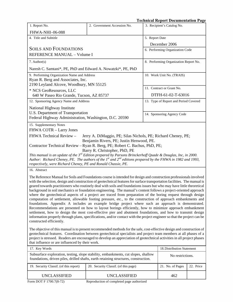
Technical Report Documentation Page 1. Report No.
2. Government Accession No. 3. Recipient’s Catalog No.
FHWA-NHI–06-088
4. Title and Subtitle 5. Report Date December 2006 6. Performing Organization Code
SOILS AND FOUNDATIONS REFERENCE MANUAL – Volume I
7. Author(s)
8. Performing Organization Report No.
Naresh C. Samtani*, PE, PhD and Edward A. Nowatzki*, PE, PhD
9. Performing Organization Name and Address 10. Work Unit No. (TRAIS) 11. Contract or Grant No.
Ryan R. Berg and Associates, Inc. 2190 Leyland Alcove, Woodbury, MN 55125 * NCS GeoResources, LLC 640 W Paseo Rio Grande, Tucson, AZ 85737
DTFH-61-02-T-63016
12. Sponsoring Agency Name and Address 13. Type of Report and Period Covered 14. Sponsoring Agency Code
National Highway Institute U.S. Department of Transportation Federal Highway Administration, Washington, D.C. 20590 15. Supplementary Notes FHWA COTR – Larry Jones FHWA Technical Review – Jerry A. DiMaggio, PE; Silas Nichols, PE; Richard Cheney, PE; Benjamin Rivers, PE; Justin Henwood, PE. Contractor Technical Review – Ryan R. Berg, PE; Robert C. Bachus, PhD, PE; Barry R. Christopher, PhD, PE This manual is an update of the 3rd Edition prepared by Parsons Brinckerhoff Quade & Douglas, Inc, in 2000. Author: Richard Cheney, PE. The authors of the 1st and 2nd editions prepared by the FHWA in 1982 and 1993, respectively, were Richard Cheney, PE and Ronald Chassie, PE. 16. Abstract The Reference Manual for Soils and Foundations course is intended for design and construction professionals involved with the selection, design and construction of geotechnical features for surface transportation facilities. The manual is geared towards practitioners who routinely deal with soils and foundations issues but who may have little theoretical background in soil mechanics or foundation engineering. The manual’s content follows a project-oriented approach where the geotechnical aspects of a project are traced from preparation of the boring request through design computation of settlement, allowable footing pressure, etc., to the construction of approach embankments and foundations. Appendix A includes an example bridge project where such an approach is demonstrated. Recommendations are presented on how to layout borings efficiently, how to minimize approach embankment settlement, how to design the most cost-effective pier and abutment foundations, and how to transmit design information properly through plans, specifications, and/or contact with the project engineer so that the project can be constructed efficiently. The objective of this manual is to present recommended methods for the safe, cost-effective design and construction of geotechnical features. Coordination between geotechnical specialists and project team members at all phases of a project is stressed. Readers are encouraged to develop an appreciation of geotechnical activities in all project phases that influence or are influenced by their work. 17. Key Words
18. Distribution Statement
Subsurface exploration, testing, slope stability, embankments, cut slopes, shallow foundations, driven piles, drilled shafts, earth retaining structures, construction.
No restrictions.
19. Security Classif. (of this report)
20. Security Classif. (of this page)
21. No. of Pages
22. Price
UNCLASSIFIED
UNCLASSIFIED
462
Form DOT F 1700.7(8-72) Reproduction of completed page authorized
FHWA NHI-06-088 6 – Slope Stability Soils and Foundations – Volume I 6 - 1 December 2006
CHAPTER 6.0 SLOPE STABILITY
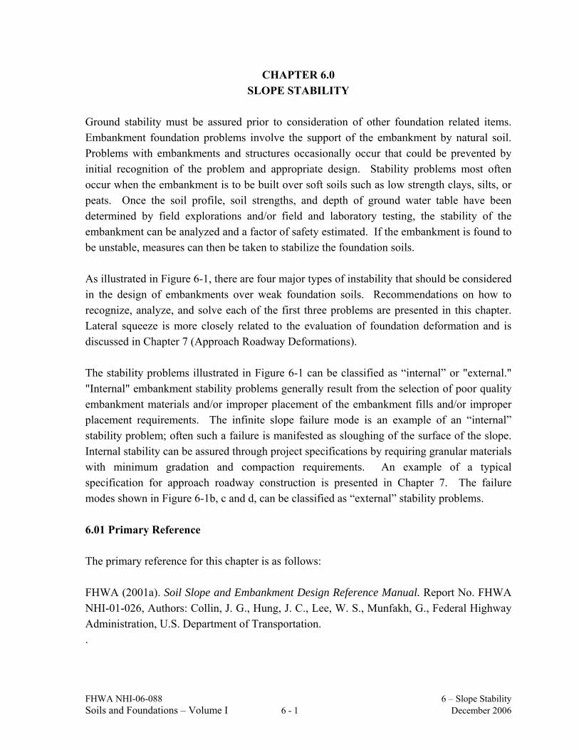
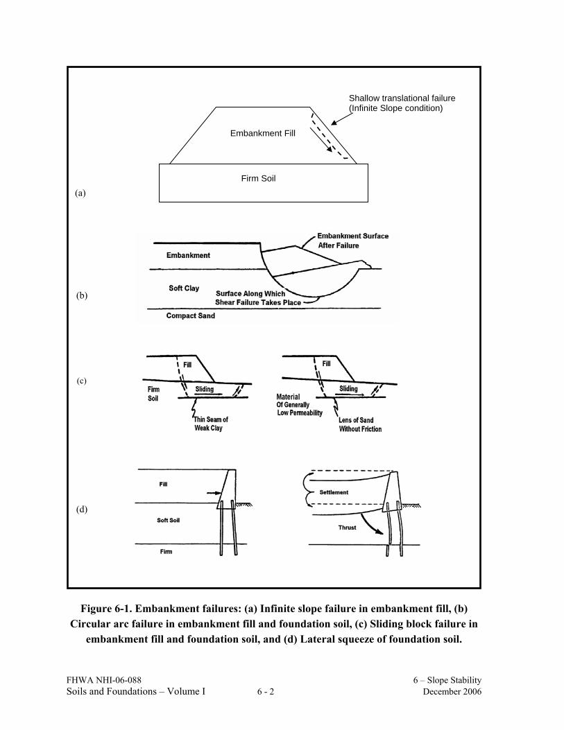
Ground stability must be assured prior to consideration of other foundation related items. Embankment foundation problems involve the support of the embankment by natural soil. Problems with embankments and structures occasionally occur that could be prevented by initial recognition of the problem and appropriate design. Stability problems most often occur when the embankment is to be built over soft soils such as low strength clays, silts, or peats. Once the soil profile, soil strengths, and depth of ground water table have been determined by field explorations and/or field and laboratory testing, the stability of the embankment can be analyzed and a factor of safety estimated. If the embankment is found to be unstable, measures can then be taken to stabilize the foundation soils. As illustrated in Figure 6-1, there are four major types of instability that should be considered in the design of embankments over weak foundation soils. Recommendations on how to recognize, analyze, and solve each of the first three problems are presented in this chapter. Lateral squeeze is more closely related to the evaluation of foundation deformation and is discussed in Chapter 7 (Approach Roadway Deformations). The stability problems illustrated in Figure 6-1 can be classified as “internal” or "external." "Internal" embankment stability problems generally result from the selection of poor quality embankment materials and/or improper placement of the embankment fills and/or improper placement requirements. The infinite slope failure mode is an example of an “internal” stability problem; often such a failure is manifested as sloughing of the surface of the slope. Internal stability can be assured through project specifications by requiring granular materials with minimum gradation and compaction requirements. An example of a typical specification for approach roadway construction is presented in Chapter 7. The failure modes shown in Figure 6-1b, c and d, can be classified as “external” stability problems. 6.01 Primary Reference The primary reference for this chapter is as follows: FHWA (2001a). Soil Slope and Embankment Design Reference Manual. Report No. FHWA NHI-01-026, Authors: Collin, J. G., Hung, J. C., Lee, W. S., Munfakh, G., Federal Highway Administration, U.S. Department of Transportation. .
FHWA NHI-06-088 6 – Slope Stability Soils and Foundations – Volume I 6 - 2 December 2006
Figure 6-1. Embankment failures: (a) Infinite slope failure in embankment fill, (b) Circular arc failure in embankment fill and foundation soil, (c) Sliding block failure in
embankment fill and foundation soil, and (d) Lateral squeeze of foundation soil.
(a)
Embankment Fill
Firm Soil
Shallow translational failure (Infinite Slope condition)
(b)
(c)
(d)
FHWA NHI-06-088 6 – Slope Stability Soils and Foundations – Volume I 6 - 3 December 2006
6.1 EFFECTS OF WATER ON SLOPE STABILITY Very soft, saturated foundation soils or ground water generally play a prominent role in geotechnical failures in general. They are certainly major factors in cut slope stability and in the stability of fill slopes involving both “internal” and “external” slope failures. The effect of water on cut and fill slope stability is briefly discussed below. • Importance of Water Next to gravity, water is the most important factor in slope stability. The effect of
gravity is known, therefore, water is the key factor in assessing slope stability. • Effect of Water on Cohesionless Soils In cohesionless soils, water does not affect the angle of internal friction (φ). The effect
of water on cohesionless soils below the water table is to decrease the intergranular (effective) stress between soil grains (σ'n), which decreases the frictional shearing resistance (τ').
• Effect of Water on Cohesive Soils Routine seasonal fluctuations in the ground water table do not usually influence either
the amount of water in the pore spaces between soil grains or the cohesion. The attractive forces between soil particles prevent water absorption unless external forces such as pile driving, disrupt the grain structure. However, certain clay minerals do react to the presence of water and cause volume changes of the clay mass.
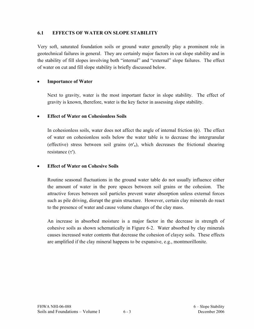
An increase in absorbed moisture is a major factor in the decrease in strength of
cohesive soils as shown schematically in Figure 6-2. Water absorbed by clay minerals causes increased water contents that decrease the cohesion of clayey soils. These effects are amplified if the clay mineral happens to be expansive, e.g., montmorillonite.
FHWA NHI-06-088 6 – Slope Stability Soils and Foundations – Volume I 6 - 4 December 2006
Cohesive Strength
Water Content
Figure 6-2. Effect of water content on cohesive strength of clay.
• Fills on Clays Excess pore water pressures are created when fills are placed on clay or silt. Provided
the applied loads do not cause the undrained shear strength of the clay or silt to be exceeded, as the excess pore water pressure dissipates consolidation occurs, and the shear strength of the clay or silt increases with time. For this reason, the factor of safety increases with time under the load of the fill.
• Cuts in Clay As a cut is made in clay the effective stress is reduced. This reduction will allow the
clay to expand and absorb water, which will lead to a decrease in the clay strength with time. For this reason, the factor of safety of a cut slope in clay may decrease with time. Cut slopes in clay should be designed by using effective strength parameters and the effective stresses that will exist in the soil after the cut is made.
• Slaking - Shales, Claystones, Siltstones, etc. Sudden moisture increase in weak rocks can produce a pore pressure increase in trapped
pore air accompanied by local expansion and strength decrease. The "slaking" or sudden disintegration of hard shales, claystones, and siltstones results from this mechanism. If placed as rock fill, these materials will tend to disintegrate into a clay soil if water is allowed to percolate through the fill. This transformation from rock to clay often leads to settlement and/or shear failure of the fill. Index tests such as the jar-slake test and the slake-durability test used to assess slaking potential are discussed in FHWA (1978).
FHWA NHI-06-088 6 – Slope Stability Soils and Foundations – Volume I 6 - 5 December 2006
6.2 DESIGN FACTOR OF SAFETY A minimum factor of safety as low as 1.25 is used for highway embankment side slopes. This value of the safety factor should be increased to a minimum of 1.30 to 1.50 for slopes whose failure would cause significant damage such as end slopes beneath bridge abutments, major retaining structures and major roadways such as regional routes, interstates, etc The selection of the design safety factor for a particular project depends on:
• The method of stability analysis used (see Section 6.4.5).
• The method used to determine the shear strength.
• The degree of confidence in the reliability of subsurface data. • The consequences of a failure. • How critical the application is.
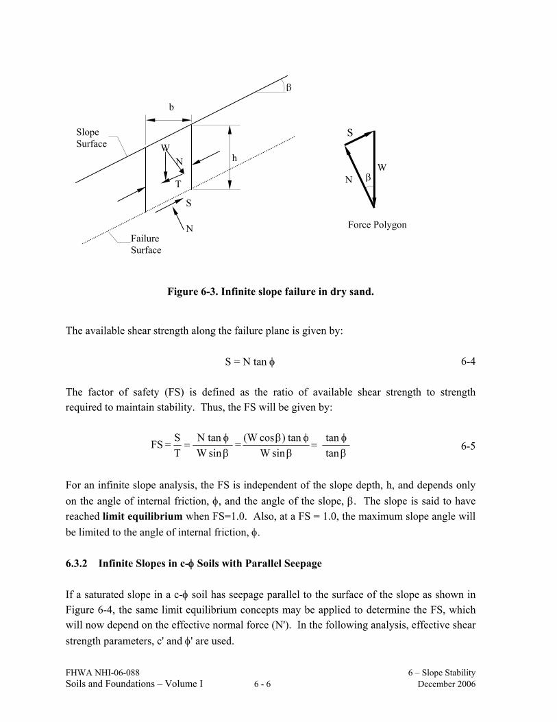
6.3 INFINITE SLOPE ANALYSIS A slope that extends for a relatively long distance and has a consistent subsurface profile may be analyzed as an infinite slope. The failure plane for this case is parallel to the surface of the slope and the limit equilibrium method can be applied readily. 6.3.1 Infinite Slopes in Dry Cohesionless Soils A typical section or “slice” through the potential failure zone of a slope in a dry cohesionless soil, e.g., dry sand, is shown in Figure 6-3, along with its free body diagram. The weight of the slice of width b and height h having a unit dimension into the page is given by:
W = γ b h 6-1 where γ is the effective unit weight of the dry soil. For a slope with angle β as shown in Figure 6-3, the normal (N) and tangential (T) force components of W are determined as follows:
N = W cos β and T = W sin β
6-26-3
FHWA NHI-06-088 6 – Slope Stability Soils and Foundations – Volume I 6 - 6 December 2006
Figure 6-3. Infinite slope failure in dry sand. The available shear strength along the failure plane is given by:
S = N tan φ 6-4 The factor of safety (FS) is defined as the ratio of available shear strength to strength required to maintain stability. Thus, the FS will be given by:
βφ
=β
φββφ
= tan
tan sinW
tan) cos(W = sinW
N tanTS = FS 6-5
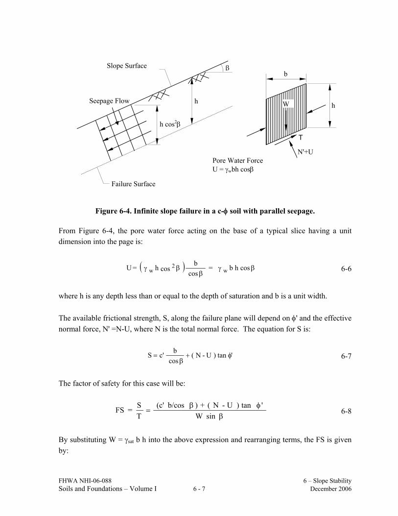
For an infinite slope analysis, the FS is independent of the slope depth, h, and depends only on the angle of internal friction, φ, and the angle of the slope, β. The slope is said to have reached limit equilibrium when FS=1.0. Also, at a FS = 1.0, the maximum slope angle will be limited to the angle of internal friction, φ. 6.3.2 Infinite Slopes in c-φ Soils with Parallel Seepage If a saturated slope in a c-φ soil has seepage parallel to the surface of the slope as shown in Figure 6-4, the same limit equilibrium concepts may be applied to determine the FS, which will now depend on the effective normal force (N'). In the following analysis, effective shear strength parameters, c' and φ' are used.
T
W
b
h
Slope Surface
Failure Surface
S
N
β
W
S
N β
Force Polygon
N
FHWA NHI-06-088 6 – Slope Stability Soils and Foundations – Volume I 6 - 7 December 2006
Figure 6-4. Infinite slope failure in a c-φ soil with parallel seepage.
From Figure 6-4, the pore water force acting on the base of a typical slice having a unit dimension into the page is:
( ) βγβ
βγ cosh b = cos
b cosh =U w 2
w 6-6
where h is any depth less than or equal to the depth of saturation and b is a unit width. The available frictional strength, S, along the failure plane will depend on φ' and the effective normal force, N' =N-U, where N is the total normal force. The equation for S is:
'tan )U -N ( cos
b c'S φ+β
= 6-7
The factor of safety for this case will be:
βφβ
= sinW
' tan) U-N ( + ) b/cos (c' TS= FS 6-8
By substituting W = γsat b h into the above expression and rearranging terms, the FS is given by:
h cos2β
Seepage Flow
Failure Surface
Slope Surface
h
β
h W
N'+U Pore Water Force U = γwbh cosβ
b
T
FHWA NHI-06-088 6 – Slope Stability Soils and Foundations – Volume I 6 - 8 December 2006
ββγ
φβγγ cos sin h
' tan) cos( ) - ( h + c' = FS
sat
2 wsat 6-9
where γ' = (γsat - γw). For c' = 0, the above expression may be simplified to:
βφ
γγ
tan'tan ' = FS
sat 6-10
From Equation 6-10 it is apparent that for a cohesionless material with parallel seepage, the FS is also independent of the slope depth, h, just as it is for a dry cohesionless material as given by Equation 6-5. The difference is that the FS for the dry material is reduced by the factor γ'/γsat for saturated cohesionless materials to account for the effect of seepage. For typical soils, this reduction will be about 50 percent in comparison to dry slopes. The above analysis can be generalized if the seepage line is assumed to be located at a normalized height, m, above the failure surface where m =z/h. In this case, the FS is:
] m + ) m - 1 ( [ cos sin h
' tan] ' m + ) m - 1 ( [ cos h + c' = FS
sat m
m 2
γγββ
φγγβ 6-11
and γsat and γm are the saturated and moist unit weights of the soil below and above the seepage line. The above equation may be readily reformulated to determine the critical depth of the failure surface in a c'-φ' soil for any seepage condition.
FHWA NHI-06-088 6 – Slope Stability Soils and Foundations – Volume I 6 - 9 December 2006
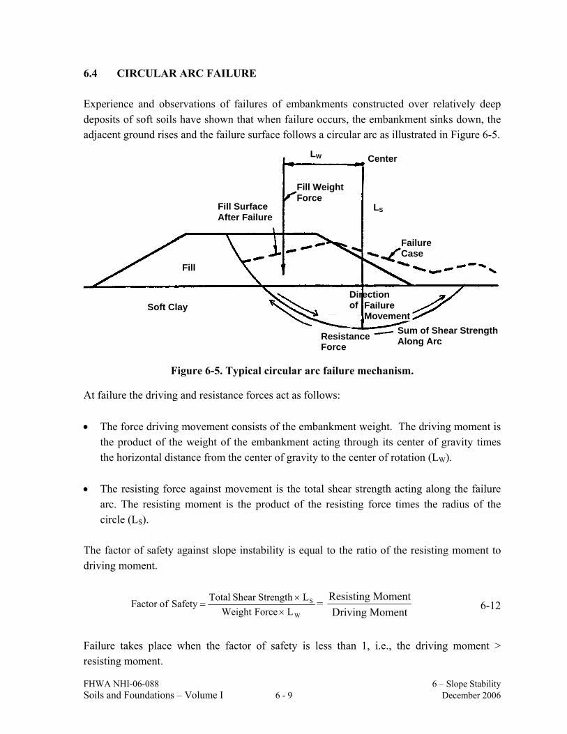
6.4 CIRCULAR ARC FAILURE Experience and observations of failures of embankments constructed over relatively deep deposits of soft soils have shown that when failure occurs, the embankment sinks down, the adjacent ground rises and the failure surface follows a circular arc as illustrated in Figure 6-5.
Figure 6-5. Typical circular arc failure mechanism.
At failure the driving and resistance forces act as follows: • The force driving movement consists of the embankment weight. The driving moment is
the product of the weight of the embankment acting through its center of gravity times the horizontal distance from the center of gravity to the center of rotation (LW).
• The resisting force against movement is the total shear strength acting along the failure
arc. The resisting moment is the product of the resisting force times the radius of the circle (LS).
The factor of safety against slope instability is equal to the ratio of the resisting moment to driving moment.
W
S
LForceWeightLStrengthShearTotalSafetyofFactor
××
= = MomentrivingDMomentResisting 6-12
Failure takes place when the factor of safety is less than 1, i.e., the driving moment > resisting moment.
Fill Surface After Failure
Fill Weight Force
Failure Case
LW Center
LS
Failure Movement
Direction ofSoft Clay
Resistance Force
Sum of Shear StrengthAlong Arc
Fill
FHWA NHI-06-088 6 – Slope Stability Soils and Foundations – Volume I 6 - 10 December 2006
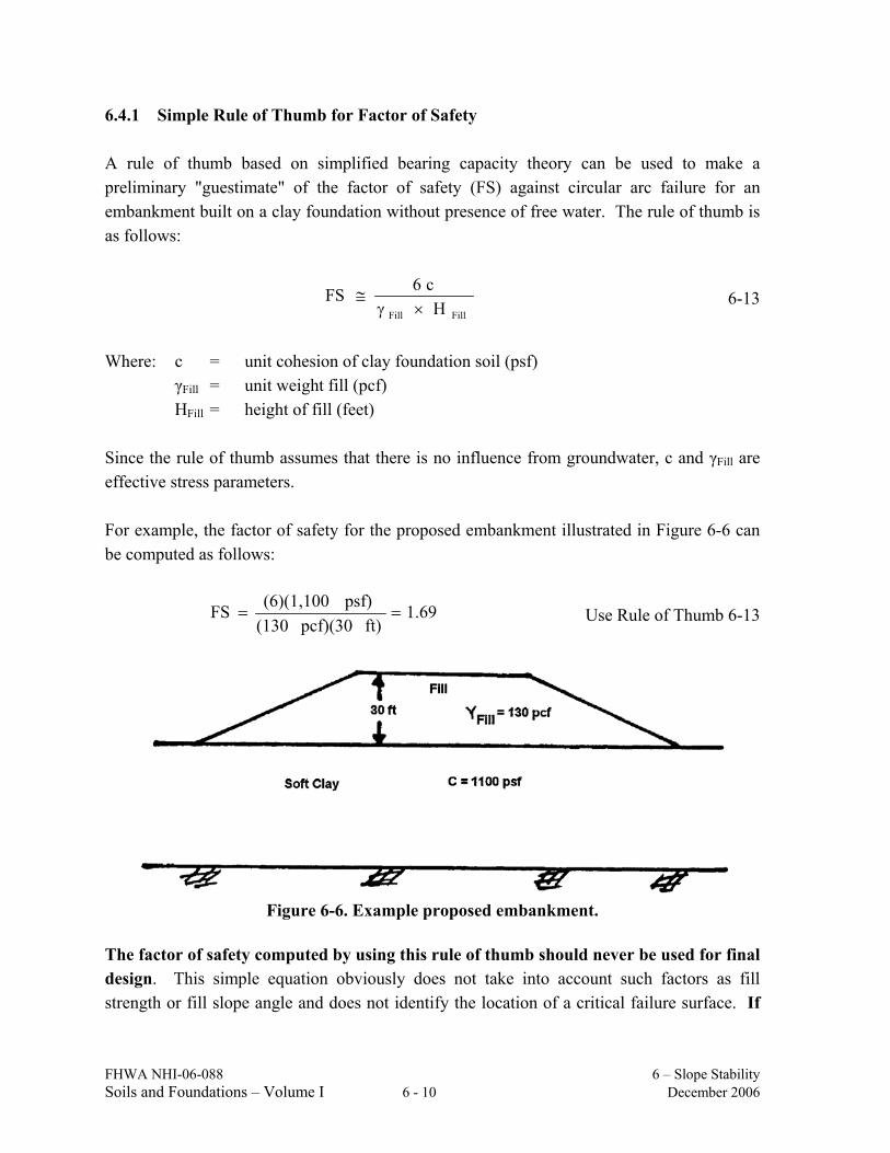
6.4.1 Simple Rule of Thumb for Factor of Safety A rule of thumb based on simplified bearing capacity theory can be used to make a preliminary "guestimate" of the factor of safety (FS) against circular arc failure for an embankment built on a clay foundation without presence of free water. The rule of thumb is as follows:
FillFill Hc6FS
×γ≅ 6-13
Where: c = unit cohesion of clay foundation soil (psf) γFill = unit weight fill (pcf) HFill = height of fill (feet) Since the rule of thumb assumes that there is no influence from groundwater, c and γFill are effective stress parameters. For example, the factor of safety for the proposed embankment illustrated in Figure 6-6 can be computed as follows:
1.69ft)pcf)(30(130
psf)(6)(1,100FS == Use Rule of Thumb 6-13
Figure 6-6. Example proposed embankment.
The factor of safety computed by using this rule of thumb should never be used for final design. This simple equation obviously does not take into account such factors as fill strength or fill slope angle and does not identify the location of a critical failure surface. If
FHWA NHI-06-088 6 – Slope Stability Soils and Foundations – Volume I 6 - 11 December 2006
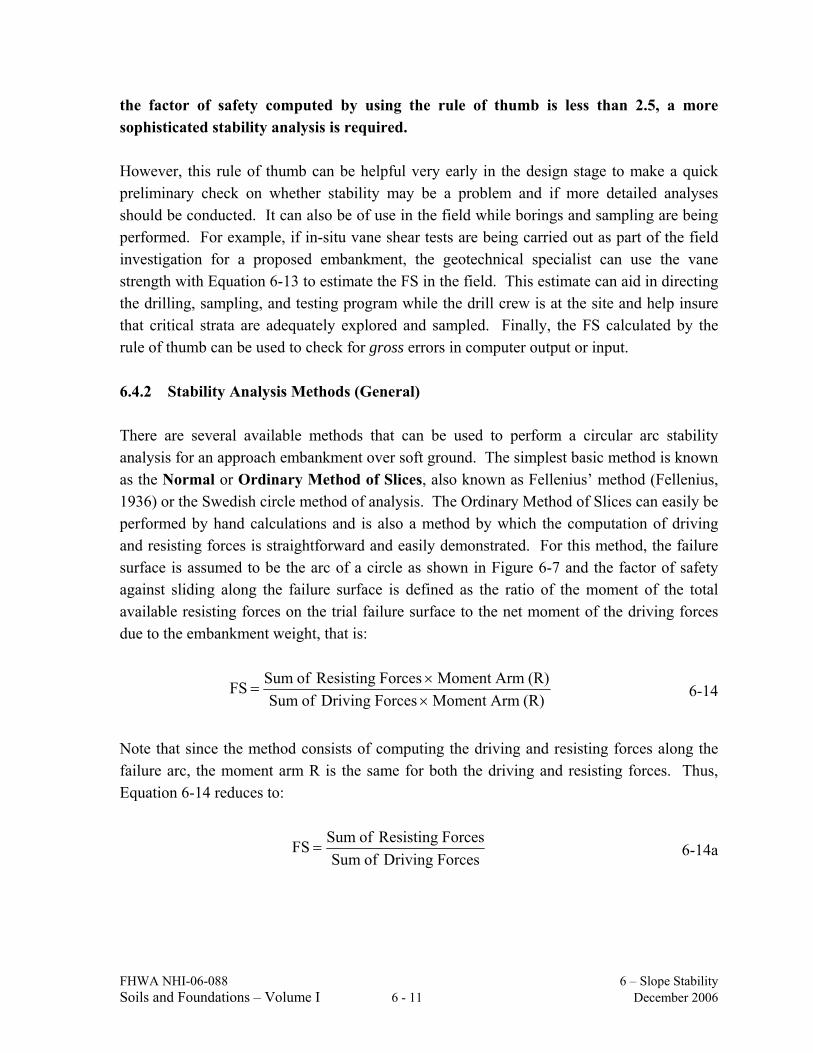
the factor of safety computed by using the rule of thumb is less than 2.5, a more sophisticated stability analysis is required. However, this rule of thumb can be helpful very early in the design stage to make a quick preliminary check on whether stability may be a problem and if more detailed analyses should be conducted. It can also be of use in the field while borings and sampling are being performed. For example, if in-situ vane shear tests are being carried out as part of the field investigation for a proposed embankment, the geotechnical specialist can use the vane strength with Equation 6-13 to estimate the FS in the field. This estimate can aid in directing the drilling, sampling, and testing program while the drill crew is at the site and help insure that critical strata are adequately explored and sampled. Finally, the FS calculated by the rule of thumb can be used to check for gross errors in computer output or input. 6.4.2 Stability Analysis Methods (General) There are several available methods that can be used to perform a circular arc stability analysis for an approach embankment over soft ground. The simplest basic method is known as the Normal or Ordinary Method of Slices, also known as Fellenius’ method (Fellenius, 1936) or the Swedish circle method of analysis. The Ordinary Method of Slices can easily be performed by hand calculations and is also a method by which the computation of driving and resisting forces is straightforward and easily demonstrated. For this method, the failure surface is assumed to be the arc of a circle as shown in Figure 6-7 and the factor of safety against sliding along the failure surface is defined as the ratio of the moment of the total available resisting forces on the trial failure surface to the net moment of the driving forces due to the embankment weight, that is:
(R)ArmMomentForcesDrivingofSum(R)ArmMomentForcesResistingofSumFS
××
= 6-14
Note that since the method consists of computing the driving and resisting forces along the failure arc, the moment arm R is the same for both the driving and resisting forces. Thus, Equation 6-14 reduces to:
ForcesDrivingofSumForcesResistingofSumFS = 6-14a
FHWA NHI-06-088 6 – Slope Stability Soils and Foundations – Volume I 6 - 12 December 2006
Figure 6-7. Geometry of Ordinary Method of Slices.
For slope stability analysis, the mass within the failure surface is divided into vertical slices as shown in Figures 6-7 and 6-8. A typical vertical slice and its free body diagram is shown in Figure 6-9 for the case where water is not a factor. The case with the presence of water is shown in Figure 6-10. The following assumptions are then made in the analysis using Ordinary Method of Slices: 1. The available shear strength of the soil can be adequately described by the
Mohr-Coulomb equation:
τ = c + (σ – u) tan φ 6-15
where: τ = effective shear strength c = cohesion component of shear strength (σ - u) tan φ = frictional component of shear strength σ = total normal stress on the failure surface at the base of a slice due to
the weight of soil and water above the failure surface u = water uplift pressure against the failure surface φ = angle of internal friction of soil tan φ = coefficient of friction along failure surface

FHWA NHI-06-088 6 – Slope Stability Soils and Foundations – Volume I 6 - 13 December 2006
2. The factor of safety is the same for all slices. 3. The factors of safety with respect to cohesion (c) and friction (tan φ) are equal. 4. Shear and normal forces on the sides of each slice are ignored. 5. The water pressure (u) is taken into account by reducing the total weight of
the slice by the water uplift force acting at the base of the slice. Equation 6-15 is expressed in terms of total strength parameters. The equation could easily have been expressed in terms of effective strength parameters. Therefore, the convention to be used in the stability analysis, be it total stress or effective stress, should be chosen and specified. In soil problems involving water, the engineer may compute the normal and tangential forces by using either total soil weights and boundary water forces (both buoyancy and unbalanced hydrostatic forces) or submerged (buoyant) soil weights and unbalanced hydrostatic forces. The results are the same. When total weight and boundary water forces are used, the equilibrium of the entire block is considered. When submerged weights and hydrostatic forces are used, the equilibrium of the mineral skeleton is considered. The total weight notation is used herein as this method is the simplest to compute. 6.4.3 Ordinary Method of Slices - Step-By-Step Computation Procedure To compute the factor of safety for an embankment by using the Ordinary Method of Slices, the step-by-step computational procedure is as follows:
Figure 6-8. Example of dividing the failure mass in slices.
FHWA NHI-06-088 6 – Slope Stability Soils and Foundations – Volume I 6 - 14 December 2006
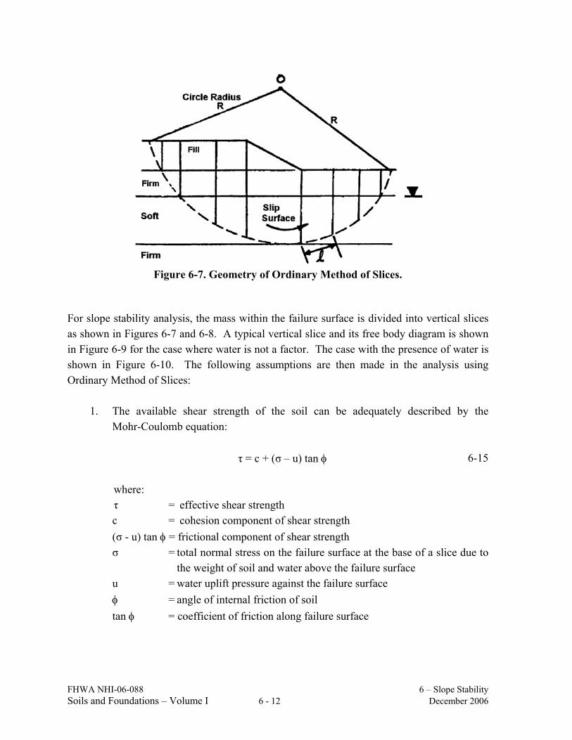
Step 1. Draw a cross-section of the embankment and foundation soil profile on a scale of either 1-inch = 10 feet or 1-inch = 20 feet scale both horizontal and vertical.
Step 2. Select a circular failure surface such as shown in Figure 6-7. Step 3. Divide the circular mass above the failure surface into 10 - 15 vertical slices as
illustrated in Figure 6-8. To simplify computation, locate the vertical sides of the slices so that the bottom of
any one slice is located entirely in a single soil layer or at the intersection of the ground water level and the circle.
Locate the top boundaries of vertical slices at breaks in the slope. The slice widths
do not have to be equal. For convenience assume a one-foot (0.3 m) thick section of embankment. This unit width simplifies computation of driving and resisting forces.
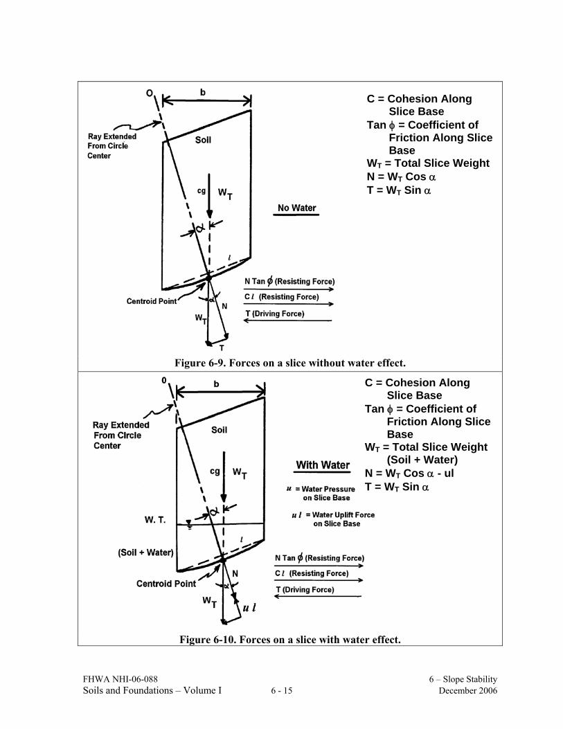
Also, as shown in Figure 6-9 and 6-10 the driving and resisting forces of each slice
act at the intersection of a vertical line drawn from the center of gravity of the slice to the failure circle to establish a centroid point on the circle. Lines (called rays) are then drawn from the center of the circle to the centroid point on the circular arc. The α angles are then measured from the vertical to each ray.
When the water table is sloping, use Equation 6-16 to calculate the water pressure
on the base of the slice:
u = hw γw cos2 αw 6-16 where: αw = slope of water table from horizontal in degrees. hw = depth from ground water surface to the centroid point on the circle. Step 4: Compute the total weight (WT) of each slice.
For illustration, the resisting and driving forces acting on individual slices with and without water pressure are shown on Figures 6-9 and 6-10.
To compute WT, use total soil unit weight, γt, both above and below the water
table.
FHWA NHI-06-088 6 – Slope Stability Soils and Foundations – Volume I 6 - 15 December 2006
Figure 6-9. Forces on a slice without water effect.
Figure 6-10. Forces on a slice with water effect.
C = Cohesion Along Slice Base
Tan φ = Coefficient of Friction Along Slice Base
WT = Total Slice Weight N = WT Cos α T = WT Sin α
C = Cohesion Along Slice Base
Tan φ = Coefficient of Friction Along Slice Base
WT = Total Slice Weight (Soil + Water)
N = WT Cos α - ul T = WT Sin α
FHWA NHI-06-088 6 – Slope Stability Soils and Foundations – Volume I 6 - 16 December 2006
WT = γt × Average Slice Height × Slice Width 6-17 For example: Assume γt = 120 pcf (18.9 kN/m3) Average height of slice = 10 ft (3 m) Slice width = 10 ft (3 m) Then for a unit thickness into the plane of the paper, WT = (120 pcf) (10 ft) (10 ft)
(1 ft) = 12,000 lbs (53.3 kN) Step 5: Compute frictional resisting force for each slice depending on location of
ground water table.
N = WT cos α 6-18a
N′ = WT cos α – ul 6-18b N = total normal force acting against the slice base N′ = effective normal force acting against the slice base WT = total weight of slice (from Step 4 above)
α = angle between vertical and line drawn from circle center to midpoint (centroid) of slice base (Note: α is also equal to the angle between the horizontal and a line tangent to the base of the slice)
u = water pressure on the base of the slice = average height of water, hw × γw. Use γw = 62.4 pcf (9.8 kN/m3)
l = arc length of slice base. To simplify computations, take l as the secant to the arc.
u l = water uplift force against base of the slice per unit thickness into the plane of the paper.
φ = internal friction angle of the soil. tan φ = coefficient of friction along base of the slice.
Note that the effect of water is to reduce the normal force against the base of the slice and thus reduce the frictional resisting force. To illustrate this reduction, take the same slice used in Step 4 and compute the friction resistance force for the slice with no water and then for the ground water table located 5 feet above the base of the slice.
FHWA NHI-06-088 6 – Slope Stability Soils and Foundations – Volume I 6 - 17 December 2006
Assume: φ = 25o α = 20o l = 11 ft (3.3 m) If there is no water in the slice, u l = 0 and Equation 6-18b reverts to Equation 6-
18a and the total frictional resistance can be computed as follows: N = WT cos α = (12,000 lbs) (cos 20o) = 11,276 lbs (50.18 kN) N tan φ = (11,276 lbs) (tan 25o) = 5,258 lbs (23.4 kN) If there is 5-ft of water above the midpoint of the slice, Equation 6-18b is used
directly and the effective frictional resistance is computed as follows: u l = (hw)(γw)(l) = (5 ft)(62.4 pcf))(11 ft)(1 ft) = 3,432 lbs (15.3 kN) N′ = WT cos α - u l = 11,276 lbs - 3,432 lbs = 7,844 lbs (34.9 kN) N′ tan φ = (7,844 lbs) (tan 25°) = 3,658 lbs (16.3 kN) Step 6: Compute cohesive resisting force for each slice. c = cohesive soil strength l = length of slice base Example: c = 200 psf (9.6 kPa) l = 11 ft (3.6 m) cl = (200 psf)(11 ft)(1 ft) = 2,200 lbs (9.8 kN) Step 7: Compute tangential driving force, T, for each slice.
T = WT sin α 6-19
T is the component of total weight of the slice, WT, acting tangent to the slice base. T is the driving force due to the weight of both soil and water in the slice.
Example: Given WT = 12,000 lbs (53.3 kN) α = 20o T = WT sin α = (12,000 lbs)(sin 20o) = 4,104 lbs (18.2 kN)

FHWA NHI-06-088 6 – Slope Stability Soils and Foundations – Volume I 6 - 18 December 2006
Step 8: Sum resisting forces and driving forces for all slices and compute factor of safety.
T1ctanN
ForcesDrivingForcesResistingFS
∑∑+φ′∑
=∑
∑= 6-20
Tabular computation forms for use in performing a method of slices stability
analysis by hand are included on Figures 6-11 and 6-12.
Slice No. b hi γi Wi ∑Wi = WT
Figure 6-11a. Tabular form for computing weights of slices.
γi = unit weight of layer i hi = height of layer at center of slice Wi = partial weight = b hi γi
∑ Wi = total weight of slice WT

FHWA NHI-06-088 6 – Slope Stability Soils and Foundations – Volume I 6 - 19 December 2006
Slice No.
WT (from Table 6-11a)
l α c φ u ul WTcosα N′ = WTcosα -ul
N′tanφ cl T= WTsinα
Σ
=αΣΣ+φ′Σ
=αΣ
Σ+φ−αΣ=
sinWcltanN
sinWcltan)ulcosW(FS
TT
T .
Legend: Refer to Figure 6-10 for definition of various slice quantities WT = Total weight of Slice (soil + water) l = Base length of the slice c = Cohesion at base of slice φ = angle of internal friction u = pore water pressure at base of slice
Figure 6-11b. Tabular form for calculating factor of safety by Ordinary Method of Slices.
WT
α
l
FHWA NHI-06-088 6 – Slope Stability Soils and Foundations – Volume I 6 - 20 December 2006
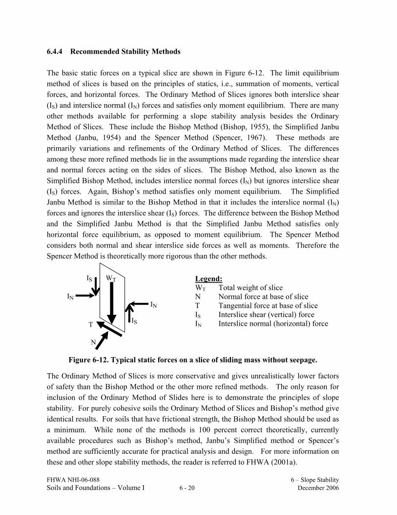
6.4.4 Recommended Stability Methods The basic static forces on a typical slice are shown in Figure 6-12. The limit equilibrium method of slices is based on the principles of statics, i.e., summation of moments, vertical forces, and horizontal forces. The Ordinary Method of Slices ignores both interslice shear (IS) and interslice normal (IN) forces and satisfies only moment equilibrium. There are many other methods available for performing a slope stability analysis besides the Ordinary Method of Slices. These include the Bishop Method (Bishop, 1955), the Simplified Janbu Method (Janbu, 1954) and the Spencer Method (Spencer, 1967). These methods are primarily variations and refinements of the Ordinary Method of Slices. The differences among these more refined methods lie in the assumptions made regarding the interslice shear and normal forces acting on the sides of slices. The Bishop Method, also known as the Simplified Bishop Method, includes interslice normal forces (IN) but ignores interslice shear (IS) forces. Again, Bishop’s method satisfies only moment equilibrium. The Simplified Janbu Method is similar to the Bishop Method in that it includes the interslice normal (IN) forces and ignores the interslice shear (IS) forces. The difference between the Bishop Method and the Simplified Janbu Method is that the Simplified Janbu Method satisfies only horizontal force equilibrium, as opposed to moment equilibrium. The Spencer Method considers both normal and shear interslice side forces as well as moments. Therefore the Spencer Method is theoretically more rigorous than the other methods.
Figure 6-12. Typical static forces on a slice of sliding mass without seepage.
The Ordinary Method of Slices is more conservative and gives unrealistically lower factors of safety than the Bishop Method or the other more refined methods. The only reason for inclusion of the Ordinary Method of Slides here is to demonstrate the principles of slope stability. For purely cohesive soils the Ordinary Method of Slices and Bishop’s method give identical results. For soils that have frictional strength, the Bishop Method should be used as a minimum. While none of the methods is 100 percent correct theoretically, currently available procedures such as Bishop’s method, Janbu’s Simplified method or Spencer’s method are sufficiently accurate for practical analysis and design. For more information on these and other slope stability methods, the reader is referred to FHWA (2001a).
IS
IS
IN IN
WT
N
T
Legend: WT Total weight of slice N Normal force at base of slice T Tangential force at base of slice IS Interslice shear (vertical) force IN Interslice normal (horizontal) force
FHWA NHI-06-088 6 – Slope Stability Soils and Foundations – Volume I 6 - 21 December 2006
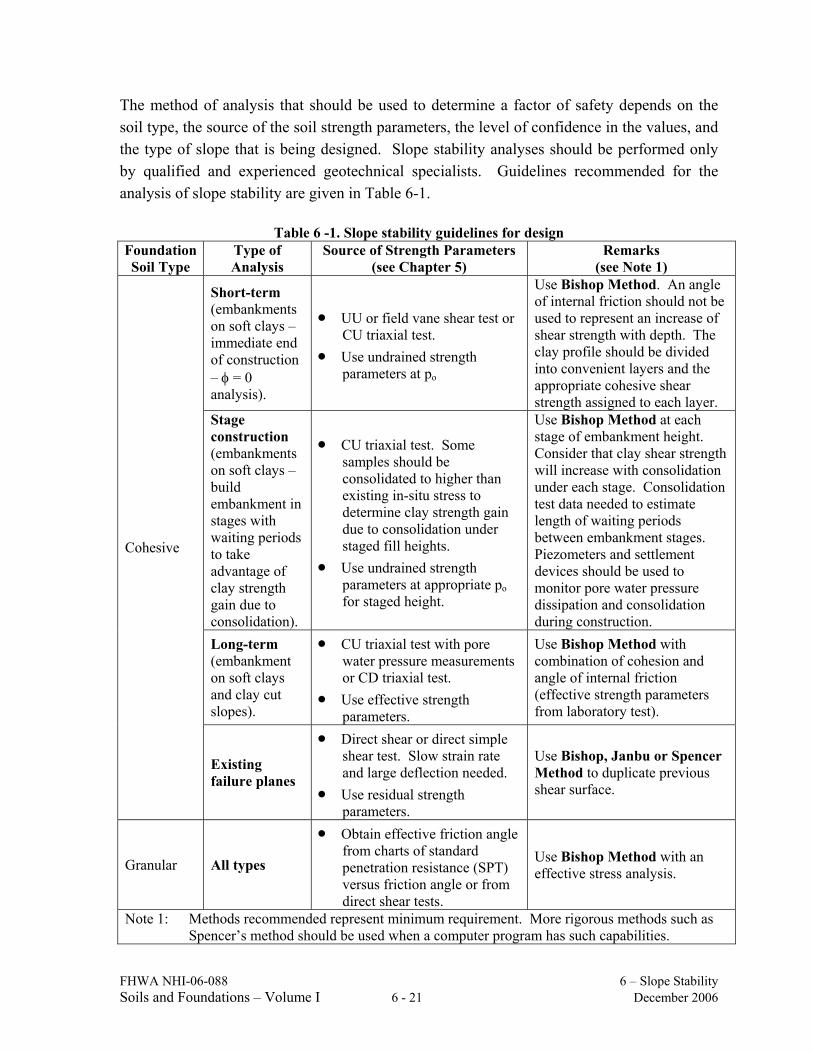
The method of analysis that should be used to determine a factor of safety depends on the soil type, the source of the soil strength parameters, the level of confidence in the values, and the type of slope that is being designed. Slope stability analyses should be performed only by qualified and experienced geotechnical specialists. Guidelines recommended for the analysis of slope stability are given in Table 6-1.
Table 6 -1. Slope stability guidelines for design
Foundation Soil Type
Type of Analysis
Source of Strength Parameters (see Chapter 5)
Remarks (see Note 1)
Short-term (embankments on soft clays – immediate end of construction – φ = 0 analysis).
• UU or field vane shear test or CU triaxial test.
• Use undrained strength parameters at po
Use Bishop Method. An angle of internal friction should not be used to represent an increase of shear strength with depth. The clay profile should be divided into convenient layers and the appropriate cohesive shear strength assigned to each layer.
Stage construction (embankments on soft clays – build embankment in stages with waiting periods to take advantage of clay strength gain due to consolidation).
• CU triaxial test. Some samples should be consolidated to higher than existing in-situ stress to determine clay strength gain due to consolidation under staged fill heights.
• Use undrained strength parameters at appropriate po for staged height.
Use Bishop Method at each stage of embankment height. Consider that clay shear strength will increase with consolidation under each stage. Consolidation test data needed to estimate length of waiting periods between embankment stages. Piezometers and settlement devices should be used to monitor pore water pressure dissipation and consolidation during construction.
Long-term (embankment on soft clays and clay cut slopes).
• CU triaxial test with pore water pressure measurements or CD triaxial test.
• Use effective strength parameters.
Use Bishop Method with combination of cohesion and angle of internal friction (effective strength parameters from laboratory test).
Cohesive
Existing failure planes
• Direct shear or direct simple shear test. Slow strain rate and large deflection needed.
• Use residual strength parameters.
Use Bishop, Janbu or Spencer Method to duplicate previous shear surface.
Granular All types
• Obtain effective friction angle from charts of standard penetration resistance (SPT) versus friction angle or from direct shear tests.
Use Bishop Method with an effective stress analysis.
Note 1: Methods recommended represent minimum requirement. More rigorous methods such as Spencer’s method should be used when a computer program has such capabilities.
FHWA NHI-06-088 6 – Slope Stability Soils and Foundations – Volume I 6 - 22 December 2006
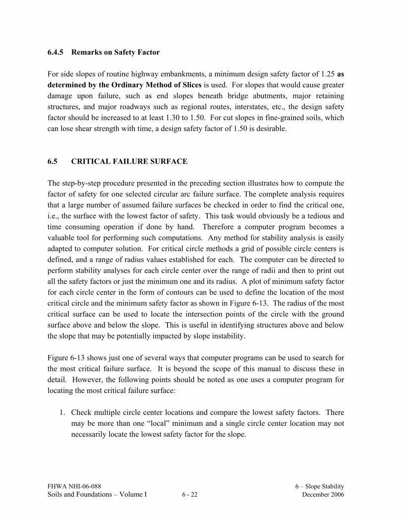
6.4.5 Remarks on Safety Factor For side slopes of routine highway embankments, a minimum design safety factor of 1.25 as determined by the Ordinary Method of Slices is used. For slopes that would cause greater damage upon failure, such as end slopes beneath bridge abutments, major retaining structures, and major roadways such as regional routes, interstates, etc., the design safety factor should be increased to at least 1.30 to 1.50. For cut slopes in fine-grained soils, which can lose shear strength with time, a design safety factor of 1.50 is desirable. 6.5 CRITICAL FAILURE SURFACE The step-by-step procedure presented in the preceding section illustrates how to compute the factor of safety for one selected circular arc failure surface. The complete analysis requires that a large number of assumed failure surfaces be checked in order to find the critical one, i.e., the surface with the lowest factor of safety. This task would obviously be a tedious and time consuming operation if done by hand. Therefore a computer program becomes a valuable tool for performing such computations. Any method for stability analysis is easily adapted to computer solution. For critical circle methods a grid of possible circle centers is defined, and a range of radius values established for each. The computer can be directed to perform stability analyses for each circle center over the range of radii and then to print out all the safety factors or just the minimum one and its radius. A plot of minimum safety factor for each circle center in the form of contours can be used to define the location of the most critical circle and the minimum safety factor as shown in Figure 6-13. The radius of the most critical surface can be used to locate the intersection points of the circle with the ground surface above and below the slope. This is useful in identifying structures above and below the slope that may be potentially impacted by slope instability. Figure 6-13 shows just one of several ways that computer programs can be used to search for the most critical failure surface. It is beyond the scope of this manual to discuss these in detail. However, the following points should be noted as one uses a computer program for locating the most critical failure surface:
1. Check multiple circle center locations and compare the lowest safety factors. There may be more than one “local” minimum and a single circle center location may not necessarily locate the lowest safety factor for the slope.
FHWA NHI-06-088 6 – Slope Stability Soils and Foundations – Volume I 6 - 23 December 2006
Figure 6-13. Location of critical circle by plotting contours of minimum safety factors
for various trial circles. 2. Search all areas of the slope to find the lowest safety factor. The designer may find
multiple areas of the slope where the safety factors are low and comparable. In this case, the designer should try to identify insignificant failure modes that lead to low safety factors for which the consequences of failure are small. This is often the case in cohesionless soils, where the lowest safety factor is found for a shallow failure plane located close the slope face.
3. Review the soil stratigraphy for “secondary” geological features such as thin
relatively weak zones where a slip surface can develop. Often, circular failure surfaces are locally modified by the presence of such weak zones. Therefore computer software capable of simulating such failures should be used. Some of the weak zones may be man-made, e.g., when new fills are not adequately keyed into existing fills for widening projects.
4. Conduct stability analyses to take into account all possible loading and unloading
schemes to which the slope might be subjected during its design life. For example, if the slope has a detention basin next to it, then it might be prudent to evaluate the effect of water on the slope, e.g., perform an analysis for a rapid drawdown condition.
5. Use the drained or undrained soil strength parameters as appropriate for the
conditions being analyzed
6. Use stability charts to develop a “feel” for the safety factor that may be anticipated. Stability charts are discussed in the next section. Such charts may also be used to verify the results of computer solutions.
FHWA NHI-06-088 6 – Slope Stability Soils and Foundations – Volume I 6 - 24 December 2006
6.6 DESIGN (STABILITY) CHARTS Slope stability charts are useful for preliminary analysis to compare alternates that may be examined in more detail later. Chart solutions also provide a quick means of checking the results of detailed analyses. Engineers are encouraged to use these charts before performing a computer analysis in order to determine the approximate value of the factor of safety. The chart solution allows some quality control and a check for the subsequent computer-generated solutions. Slope stability charts are also used to back-calculate strength values for failed slopes, such as landslides, to aid in planning remedial measures. In back-calculating strength values a factor of safety of unity is assumed for the conditions at failure. Since soil strength often involves both cohesion and friction, there are no unique values that will give a factor of safety equal to one. Therefore, selection of the most appropriate values of cohesion and friction depends on local experience and judgment. Since the friction angle is usually within a narrow range for many types of soils and can be obtained by laboratory tests with a certain degree of confidence, it is generally fixed for the back-calculations in practice and the value of cohesion is varied until a factor of safety of one is obtained. The major shortcoming in using design charts is that most charts are for ideal, homogeneous soil conditions that are not typically encountered in practice. Design charts have been devised with the following general assumptions:
1. Two-dimensional limit equilibrium analysis. 2. Simple homogeneous slopes. 3. Slip surfaces of circular shapes only.
It is imperative that the user understands the underlying assumptions for the charts before using them for the design of slopes. Regardless of the above shortcomings, many practicing engineers use these charts for non-homogeneous and non-uniform slopes with different geometrical configurations. To do this correctly, one must use an average slope inclination and weighted averages of c, φ, or c', φ' or cu calculated on the basis of the proportional length of slip surface passing through different relatively homogeneous layers. Such a procedure is extremely useful for preliminary analyses and saves time and expense. In most cases, the results are checked by performing detailed analyses using more suitable and accurate methods, for example, one of the methods of slices discussed previously.
FHWA NHI-06-088 6 – Slope Stability Soils and Foundations – Volume I 6 - 25 December 2006
6.6.1 Historical Background Some of the first slope stability charts were published by Taylor (1948). Since then various charts were developed by many investigators. Two of the most common stability charts are presented in this manual. These were developed by Taylor (1948) and Janbu (1968). 6.6.2 Taylor’s Stability Charts Taylor’s Stability Charts (Taylor, 1948) were derived from solutions based on circular failure surfaces for the stability of simple, homogeneous, finite slopes without seepage (i.e., condition of effective stress). The general equations that Taylor developed as the basis for his stability charts are relationships between the height (H) and inclination (β) of the slope, the unit weight of the soil (γ), and the values of the soil’s developed (mobilized) shear strength parameters, cd and φd. These developed (mobilized) quantities are as follows:
φ
φ ′=φ
′=
Ftantan;
Fcc d
cd 6-21
Where Fc is the average factor of safety with respect to cohesion and Fφ, is the average factor of safety with respect to friction angle, i.e., φd = arctan (tan φ′/ Fφ). As an approximation, the following equation may be used for the developed friction angle:
φ
φ ′≈φ
Fd 6-22
However, for soils possessing both frictional and cohesive components of strength, the factor of safety in slope stability analyses generally refers to the overall factor of safety with respect to shearing strength, FS, which equals τ/τd where τ = shear strength and τd = the developed (mobilized) shear strength. Therefore, the general Mohr-Coulomb expression for developed shear strength in terms of combined factors of safety is:
φ
φ′+′
=τ
=τF
tanσFc
FS cd 6-23
Equation 6-23 can be re-written in terms of developed shear strength parameters as follows:
ddd tanσcτ φ′+= 6-24
FHWA NHI-06-088 6 – Slope Stability Soils and Foundations – Volume I 6 - 26 December 2006
There are an unlimited number of combinations of Fc and Fφ that can result in a given value of FS. However, Equations 6-21 and 6-23 suggest that for the case where the value of Fc = Fφ, the factor of safety with respect to shearing strength, FS, also equals that value. The importance of this condition will be illustrated in Section 6.6.2.1 by an example problem. To simplify the determination of the factor of safety, Taylor calculated the stability of a large number of slopes over a wide range of slope angles and developed friction angles, φd. He represented the results by a dimensionless number that he called the “Stability Number,” Ns, which he defined as follows:
γHFc
γHcN
c
ds
′== 6-25
Equation 6-25 can be rearranged to provide an expression for Fc as a function of the Stability Number and three variables, c′, H and γ, as follows:
γHNcFs
c′
= 6-26
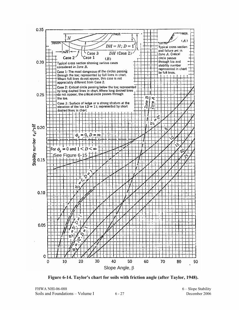
Taylor published his results in the form of curves that give the relationship between Ns and slope angle, β, for various values of developed friction angles, φd, as shown in Figure 6-14. Note that factors of safety do not appear in the chart. The chart is divided into two zones, A and B. As shown in the inset for Zone A, the critical circle for steep slopes passes through the toe of the slope with the lowest point on the failure arc at the toe of the slope. As shown in the inset for Zone B, for shallower slopes the lowest point of the critical circle is not at the toe, and three cases must be considered as follows:
• Case 2: For shallow slope angles or small developed friction angles the critical circle may pass below the toe of the slope. This condition corresponds to Case 2 in the inset for Zone B. The values of Ns for this case are given in the chart by the long dashed curves.
FHWA NHI-06-088 6 – Slope Stability Soils and Foundations – Volume I 6 - 27 December 2006
Figure 6-14. Taylor's chart for soils with friction angle (after Taylor, 1948).
See Figure 6-15
Slope Angle, β
FHWA NHI-06-088 6 – Slope Stability Soils and Foundations – Volume I 6 - 28 December 2006
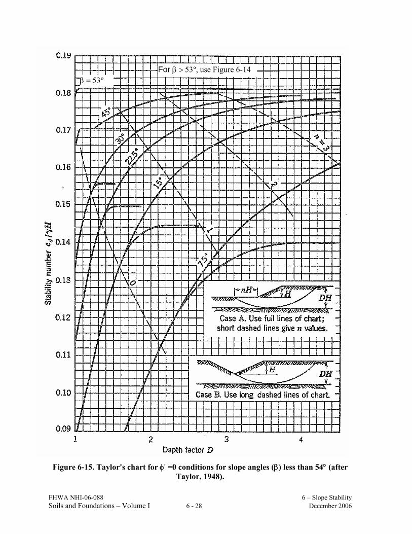
Figure 6-15. Taylor's chart for φ' =0 conditions for slope angles (β) less than 54° (after
Taylor, 1948).
β = 53º For β > 53º, use Figure 6-14
FHWA NHI-06-088 6 – Slope Stability Soils and Foundations – Volume I 6 - 29 December 2006
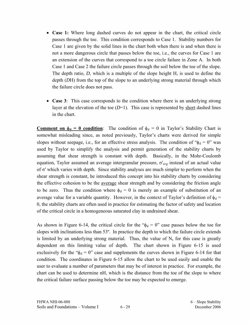
• Case 1: Where long dashed curves do not appear in the chart, the critical circle passes through the toe. This condition corresponds to Case 1. Stability numbers for Case 1 are given by the solid lines in the chart both when there is and when there is not a more dangerous circle that passes below the toe, i.e., the curves for Case 1 are an extension of the curves that correspond to a toe circle failure in Zone A. In both Case 1 and Case 2 the failure circle passes through the soil below the toe of the slope. The depth ratio, D, which is a multiple of the slope height H, is used to define the depth (DH) from the top of the slope to an underlying strong material through which the failure circle does not pass.
• Case 3: This case corresponds to the condition where there is an underlying strong
layer at the elevation of the toe (D=1). This case is represented by short dashed lines in the chart.
Comment on φd = 0 condition: The condition of φd = 0 in Taylor’s Stability Chart is somewhat misleading since, as noted previously, Taylor’s charts were derived for simple slopes without seepage, i.e., for an effective stress analysis. The condition of “φd = 0” was used by Taylor to simplify the analysis and permit generation of the stability charts by assuming that shear strength is constant with depth. Basically, in the Mohr-Coulomb equation, Taylor assumed an average intergranular pressure, σ′avg instead of an actual value of σ′ which varies with depth. Since stability analyses are much simpler to perform when the shear strength is constant, he introduced this concept into his stability charts by considering the effective cohesion to be the average shear strength and by considering the friction angle to be zero. Thus the condition where φd = 0 is merely an example of substitution of an average value for a variable quantity. However, in the context of Taylor’s definition of φd = 0, the stability charts are often used in practice for estimating the factor of safety and location of the critical circle in a homogeneous saturated clay in undrained shear. As shown in Figure 6-14, the critical circle for the “φd = 0” case passes below the toe for slopes with inclinations less than 53º. In practice the depth to which the failure circle extends is limited by an underlying strong material. Thus, the value of Ns for this case is greatly dependent on this limiting value of depth. The chart shown in Figure 6-15 is used exclusively for the “φd = 0” case and supplements the curves shown in Figure 6-14 for that condition. The coordinates in Figure 6-15 allow the chart to be used easily and enable the user to evaluate a number of parameters that may be of interest in practice. For example, the chart can be used to determine nH, which is the distance from the toe of the slope to where the critical failure surface passing below the toe may be expected to emerge.
FHWA NHI-06-088 6 – Slope Stability Soils and Foundations – Volume I 6 - 30 December 2006
6.6.2.1 Determination of the Factor of Safety for a Slope As indicated in Section 6.6.2, in order to use Taylor’s charts to determine the minimum overall factor of safety with respect to shear strength for a slope of given height H and inclination β having soil properties γ, c′ and φ′, the condition FS = Fc = Fφ must be satisfied. The general computational approach is as follows:
1. Assume a reasonable value for the common factors of safety FS = Fc = Fφ. 2. Use Equations 6-21 to calculate the corresponding values of cd and φd. 3. For the given value of β and the calculated value of φd, read the corresponding value
of the stability number Ns from Figure 6-14. 4. Use an inverted form of Equation 6-26 to calculate the slope height H corresponding
to the assumed factor of safety. 5. If the calculated value of H is within an acceptable distance of the actual height, e.g.,
± 0.5 feet, the assumed value of the common factor of safety represents the minimum overall factor of safety of the slope with respect to shear strength, Fs.
6. If the calculated value of H is not within the desired acceptable range, the process is repeated with a new assumed value of the common factor of safety until the recomputed value of H falls within that range.
7. The new assumed value of the common factor of safety for subsequent iterations is generally less than the previously chosen value if the calculated value of H is less than the actual value of H. Conversely, a. larger value of the new common factor of safety is assumed if the calculated value of H is greater than the actual value of H.
The use of Taylor’s chart is illustrated by the following example. Example 6-1: Determine the factor of safety for a 30 ft high fill slope. The slope angle is
30º. The fill is constructed with soil having the following properties: Total unit weight, γ = 120 pcf; Effective cohesion, c′ = 500 psf Effective friction angle, φ′ = 20º Solution: First assume a common factor of safety of 1.6 for both cohesion and friction angle so that Fc = Fφ = 1.6. Since Fφ = 1.6, the developed friction angle, φd, can be computed as follows:
oo
d 12.81.6
20tanarctanF
tanarctan =⎟⎟⎠
⎞⎜⎜⎝
⎛=⎟
⎟⎠
⎞⎜⎜⎝
⎛ φ ′=φ
φ
FHWA NHI-06-088 6 – Slope Stability Soils and Foundations – Volume I 6 - 31 December 2006
For φd = 12.8º, and β = 30º, the value of the stability number Ns from Figure 6-14 is approximately 0.065. Thus, from Equation 6-26
(H)pcf)(120(1.6)psf5000.065 =
or
(0.065)pcf)(120(1.6)psf500H = = 40.1 ft
Since computed height H = 40.1 ft is greater than the actual height of 30-ft, the value of the common safety factor must be greater than 1.6. Assume Fc = Fφ = 1.9 and recompute as follows: If Fφ = 1.9, then φd = 10.8º and Ns from Figure 6-14 is approximately 0.073 based on which the recomputed value of H is as follows:
(0.073)pcf)(120(1.9)psf500H = = 30.04 ft
The height of 30.04 ft is virtually identical to the correct height of 30 ft. Therefore, the minimum factor of safety with respect to shearing strength is approximately 1.9. Alternate Graphical Approach An alternate graphical approach for determining the minimum factor of safety with respect to shearing strength is also available. The procedure is as follows:
1. Assume a reasonable value for Fφ and calculate φd. 2. For the given value of β and the calculated value of φd read the corresponding value
of the stability number Ns from Figure 6-14. 3. Use Equation 6-26 to calculate Fc 4. Repeat the process for at least two other assumed values of Fφ over a range of
expected factors of safety so that at least three pairs of Fφ and Fc are obtained. 5. Plot the calculated points on Fc versus Fφ coordinates and draw a curve through the
points. 6. Draw a line through the origin that represents Fc = Fφ. 7. The minimum overall factor of safety of the slope with respect to shear strength is the
value of factor of safety at the intersection of the calculated with the Fc = Fφ line.
FHWA NHI-06-088 6 – Slope Stability Soils and Foundations – Volume I 6 - 32 December 2006
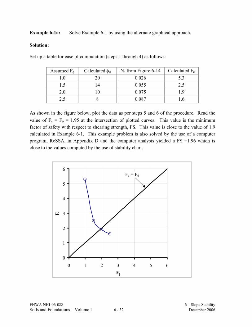
Example 6-1a: Solve Example 6-1 by using the alternate graphical approach. Solution: Set up a table for ease of computation (steps 1 through 4) as follows:
Assumed Fφ Calculated φd Ns from Figure 6-14 Calculated Fc 1.0 20 0.026 5.3 1.5 14 0.055 2.5 2.0 10 0.075 1.9 2.5 8 0.087 1.6
As shown in the figure below, plot the data as per steps 5 and 6 of the procedure. Read the value of Fc = Fφ = 1.95 at the intersection of plotted curves. This value is the minimum factor of safety with respect to shearing strength, FS. This value is close to the value of 1.9 calculated in Example 6-1. This example problem is also solved by the use of a computer program, ReSSA, in Appendix D and the computer analysis yielded a FS =1.96 which is close to the values computed by the use of stability chart.
0
1
2
3
4
5
6
0 1 2 3 4 5 6Fφ
F c
Fc = Fφ
FHWA NHI-06-088 6 – Slope Stability Soils and Foundations – Volume I 6 - 33 December 2006
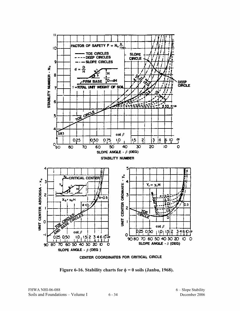
6.6.3 Janbu’s Stability Charts Janbu (1968) published stability charts for slopes in soils with uniform strength for φ = 0 and φ > 0 conditions. These charts are presented in Figures 6-16 through 6-19. This series of charts accounts for several different conditions and provides factors for surcharge loading at the top of the slope, submergence, and tension cracks that can be expected to influence the design of typical highway slopes. The stability chart for slopes in soils with uniform shear strength throughout the depth of the layer and with φ = 0 is shown in Figure 6-16. Charts for correction factors for the conditions when surcharge loads, submergence and tension cracks are present are shown in Figures 6-17 through 6-19. Step-by-step guidance for the use Janbu’s charts follows. Steps for using Janbu’s Charts on Figures 6-16 through 6-19, for φ = 0 material. Step 1. Use the chart at the bottom of Figure 6-16 to determine the position of the center
of the critical circle, which is located at a coordinate point defined by Xo, Yo with respect to a cartesian coordinate system whose origin is at the toe of the slope. Following are some guidelines that can be used to identify the critical center: o For slopes steeper than 53°, the critical circle passes through the toe. For
slopes flatter than 53°, the critical circle passes below the toe. o In addition to the toe circle, at least four circles with different depths below
the toe, D, should be analyzed to ensure that the actual minimum factor of safety and the actual critical circle have been found. The following suggestions may be used to select the circles (Duncan and Wright, 2005):
If there is water outside the slope, a circle passing above the water may be critical.
If a soil layer is weaker than the one above it, the critical circle may extend into the lower (weaker) layer. This applies to layers both above and below the toe.
If a soil layer is stronger than the one above it, the critical circle may be tangent to the top of the stronger layer.
For each of the assumed circles, perform Steps 2 to 6.
FHWA NHI-06-088 6 – Slope Stability Soils and Foundations – Volume I 6 - 34 December 2006
Figure 6-16. Stability charts for φ = 0 soils (Janbu, 1968).
FHWA NHI-06-088 6 – Slope Stability Soils and Foundations – Volume I 6 - 35 December 2006
Step 2. Using the assumed critical circle as a guide, estimate the average value of strength, c, by calculating the weighted average of the strengths along the failure surface. The number of degrees intersected along the arc by each soil layer as a percentage of the entire angle subtended by the arc is used as the weighting factor.
Step 3. Calculate the depth factor, d where d = D/H. (Note that the depth factor, d, for
Janbu’s charts is different from the depth ratio D for Taylor’s chart.) Step 4. Calculate Pd by using the following equation:
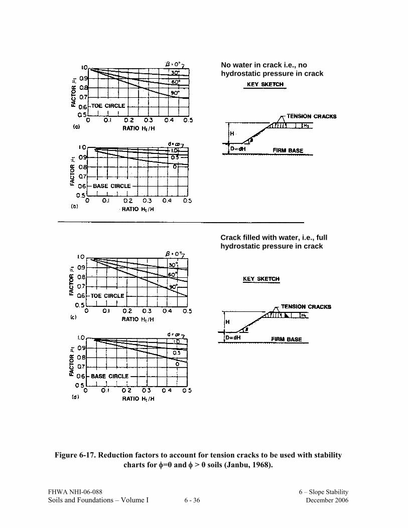
Pd = (γH + q - γwHw)/( µt µqµw) 6-27 where: q = surcharge load γw = unit weight of water Hw = depth of water outside the slope µt = tension crack correction factor (Figure 6-17) µq = surcharge correction factor (Figure 6-18, top) µw = submergence correction factor (Figure 6-18, bottom) Step 5. Use the chart at the top of Figure 6-16 to determine the value of the stability
number, No, which depends on the slope angle β, and the value of d. Step 6. Calculate the factor of safety (FS) by using the following equation:
FS = Noc/Pd 6-28 Step 7. Repeat Steps 2 to 6 for all the circles assumed in Step 1. Compare the FS to
obtain the most critical circle as the circle with the lowest FS. If it appears that the minimum FS is for a circle close to the toe, i.e., d=0, then it is prudent to check if the critical failure surface is within the height of the slope, H. In this case, the toe of the slope is adjusted to the point of intersection of assumed circle with the slope and all dimensions, (i.e., D, H, and Hw) are adjusted accordingly in the calculations and steps 1 to 6 are repeated (Duncan and Wright, 2005).
FHWA NHI-06-088 6 – Slope Stability Soils and Foundations – Volume I 6 - 36 December 2006
Figure 6-17. Reduction factors to account for tension cracks to be used with stability charts for φ=0 and φ > 0 soils (Janbu, 1968).
Crack filled with water, i.e., full hydrostatic pressure in crack
No water in crack i.e., no hydrostatic pressure in crack
FHWA NHI-06-088 6 – Slope Stability Soils and Foundations – Volume I 6 - 37 December 2006
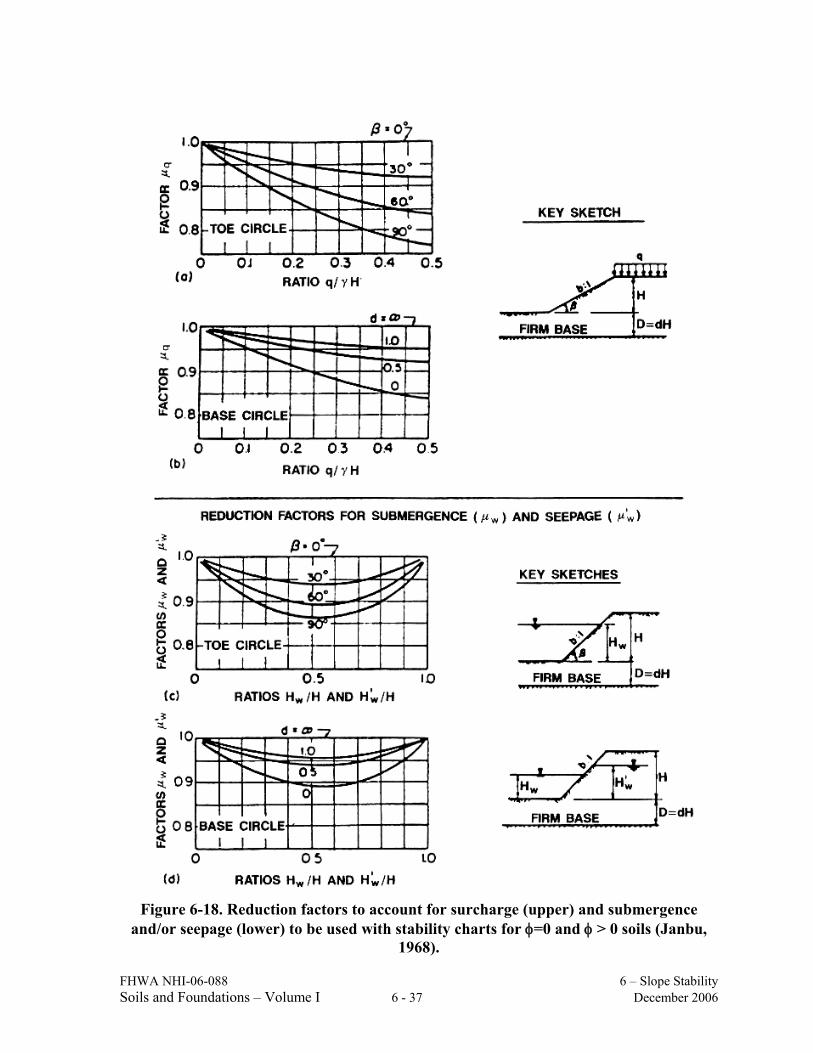
Figure 6-18. Reduction factors to account for surcharge (upper) and submergence
and/or seepage (lower) to be used with stability charts for φ=0 and φ > 0 soils (Janbu, 1968).
FHWA NHI-06-088 6 – Slope Stability Soils and Foundations – Volume I 6 - 38 December 2006
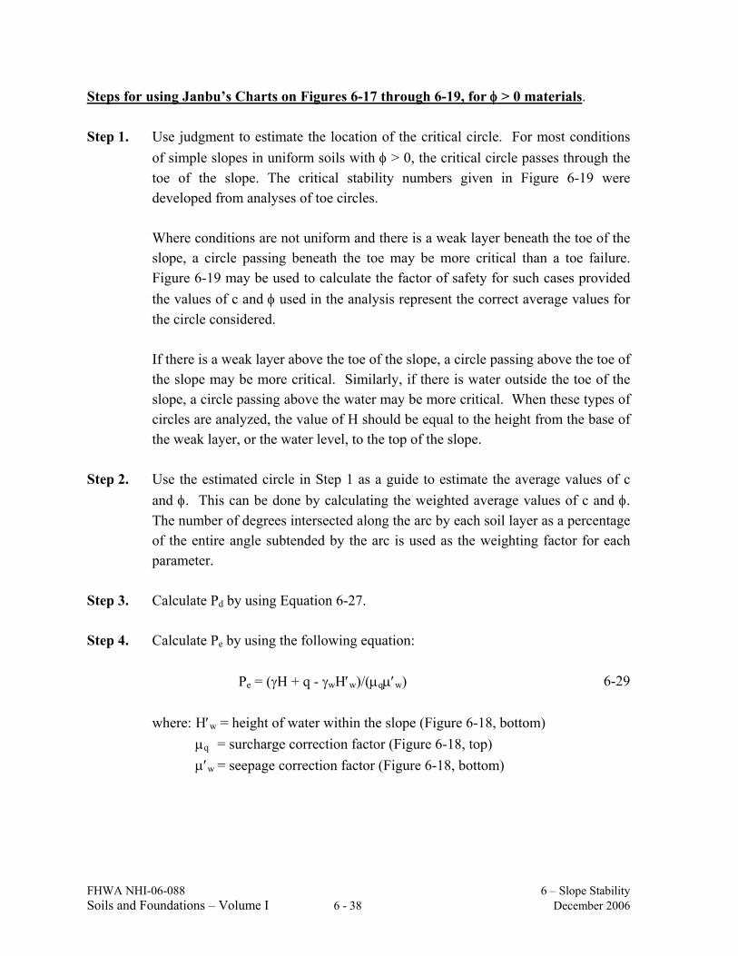
Steps for using Janbu’s Charts on Figures 6-17 through 6-19, for φ > 0 materials. Step 1. Use judgment to estimate the location of the critical circle. For most conditions
of simple slopes in uniform soils with φ > 0, the critical circle passes through the toe of the slope. The critical stability numbers given in Figure 6-19 were developed from analyses of toe circles.
Where conditions are not uniform and there is a weak layer beneath the toe of the
slope, a circle passing beneath the toe may be more critical than a toe failure. Figure 6-19 may be used to calculate the factor of safety for such cases provided the values of c and φ used in the analysis represent the correct average values for the circle considered.
If there is a weak layer above the toe of the slope, a circle passing above the toe of
the slope may be more critical. Similarly, if there is water outside the toe of the slope, a circle passing above the water may be more critical. When these types of circles are analyzed, the value of H should be equal to the height from the base of the weak layer, or the water level, to the top of the slope.
Step 2. Use the estimated circle in Step 1 as a guide to estimate the average values of c
and φ. This can be done by calculating the weighted average values of c and φ. The number of degrees intersected along the arc by each soil layer as a percentage of the entire angle subtended by the arc is used as the weighting factor for each parameter.
Step 3. Calculate Pd by using Equation 6-27. Step 4. Calculate Pe by using the following equation:
Pe = (γH + q - γwH′w)/(µqµ′w) 6-29 where: H′w = height of water within the slope (Figure 6-18, bottom) µq = surcharge correction factor (Figure 6-18, top) µ′w = seepage correction factor (Figure 6-18, bottom)
FHWA NHI-06-088 6 – Slope Stability Soils and Foundations – Volume I 6 - 39 December 2006
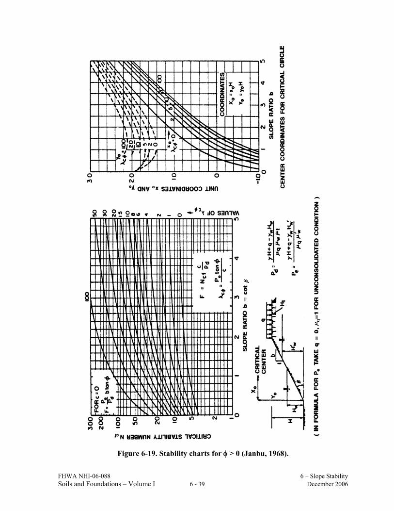
Figure 6-19. Stability charts for φ > 0 (Janbu, 1968).
FHWA NHI-06-088 6 – Slope Stability Soils and Foundations – Volume I 6 - 40 December 2006
Step 5. Calculate the dimensionless parameter λCφ by using the following equation:
λCφ = Pe tanφ/c 6-30 For c=0, λCφ is infinite therefore skip to Step 6. Step 6. Use the chart in Figure 6-19 to determine the value of the critical stability
number, Ncf, which is dependent on the slope angle, β, and the value of λCφ. Step 7. Calculate the factor of safety for the slope as follows:
For c > 0 FS = Ncf c/ Pd 6-31For c = 0 FS = Pe b tan φ/ Pd 6-32
Step 8. Determine the actual location of the critical circle by using the chart on the right
side of Figure 6-19. The center of the circle is located at a coordinate point defined by Xo, Yo with respect to a cartesian coordinate system whose origin is at the toe of the slope. The circle passes through the toe of the slope (the origin), except for slopes flatter than 53°, where the critical circle passes tangent to the top of firm soil or rock. If the critical circle is much different from the one assumed in Step 1 for the purpose of determining the average strength, Steps 2 through 8 should be repeated.
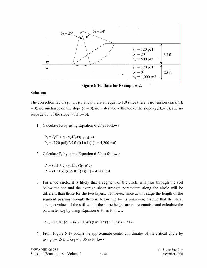
If a slope contains more than one soil layer, it may be necessary to calculate the factor of safety for circles at more than one depth. If the underlying soil layer is weaker than the layer above it, the critical circle will extend into the lower layer, and either a toe circle or a deep circle within this layer will be critical. If the underlying soil layer is stronger than the layer above it, the critical circle may or may not extend into the lower layer, depending on the relative strengths of the two layers. Both possibilities should be examined (Duncan and Wright, 2005). The use of Janbu’s charts is illustrated by the following example. Example 6-2: Figure 6-20 shows a 35 ft high slope with a grade of 1.5H:1V. The soil
properties within the slope and under it are shown on the figure. Groundwater is immediately under the slope. Calculate the factor of safety for a toe circle by using total stress analysis based on the soil properties shown. (Note: The circle in Figure 6-20 is plotted in Step 5 of the solution.)
FHWA NHI-06-088 6 – Slope Stability Soils and Foundations – Volume I 6 - 41 December 2006
Solution: The correction factors µt, µq, µw and µ′w are all equal to 1.0 since there is no tension crack (Ht = 0), no surcharge on the slope (q = 0), no water above the toe of the slope (γwHw= 0), and no seepage out of the slope (γwH′w= 0).
1. Calculate Pd by using Equation 6-27 as follows:
Pd = (γH + q - γwHw)/(µt µqµw) Pd = (120 pcf)(35 ft)/[(1)(1)(1)] = 4,200 psf
2. Calculate Pe by using Equation 6-29 as follows:
Pe = (γH + q - γwH′w)/(µqµ′w) Pe = (120 pcf)(35 ft)/[(1)(1)] = 4,200 psf
3. For a toe circle, it is likely that a segment of the circle will pass through the soil
below the toe and the average shear strength parameters along the circle will be different than those for the two layers. However, since at this stage the length of the segment passing through the soil below the toe is unknown, assume that the shear strength values of the soil within the slope height are representative and calculate the parameter λCφ by using Equation 6-30 as follows:
λCφ = Pe tanφ/c = (4,200 psf) (tan 20º)/(500 psf) = 3.06
4. From Figure 6-19 obtain the approximate center coordinates of the critical circle by
using b=1.5 and λCφ = 3.06 as follows
35 ft
25 ft
δ2 = 29º δ1 = 54º
γt = 120 pcf φu = 20º cu = 500 psf
γt = 120 pcf φu = 0º cu = 1,000 psf
Figure 6-20. Data for Example 6-2.
FHWA NHI-06-088 6 – Slope Stability Soils and Foundations – Volume I 6 - 42 December 2006
xo ≈ 0.4 yo ≈ 1.6 Thus, Xo = (H)(xo) = (35 ft) (0.4) = 14 ft Yo = (H)(yo) = (35 ft) (1.6) = 56 ft
5. Plot the critical circle on the given slope, as shown in Figure 6-20. Note that the
subtended angles for the failure circle within the slope and the foundation are δ1= 54º and δ2 = 29 degrees, respectively.
6. Calculate cav, tan φav and λCφ based on the angular distribution of the failure surface
within the slope and foundation soil using δ1 and δ2 as follows:
cav = [(54º) (500 psf) + (29º) (1,000 psf)] / (54º+29º) = 674.7 psf tan φav = [(54º) (tan 20º) + (29º) (tan 0º)] / (54º+29º) = 0.236 (or φav = 13.3º) Thus, according to Equation 6-30; λCφ = Pe tanφ/c = (4,200 psf) (0.236)/(674.7 psf) = 1.47 ≈ 1.5
7. From Figure 6-19 obtain the center coordinates of the critical circle by using b=1.5
and λCφ = 1.5 as follows
xo ≈ 0.5 yo ≈ 1.55 Thus, Xo = (H)(xo) = (35 ft) (0.5) = 17.5 ft Yo = (H)(yo) = (35 ft) (1.55) = 54.3 ft
This circle is close to the circle obtained in the previous iteration, so retain λCφ = 1.5
and cav = 674.7 psf .
8. From Figure 6-19, obtain Ncf = 10.0 for b = 1.5 and λCφ = 1.5.
9. Calculate the factor of safety, FS, by using Equation 6-28 as follows :
FS = Noc/Pd = (10) (674.7 psf) / (4,200 psf)
FS = 1.61 This calculation sequence is only for a given circle. This sequence is repeated for
several circles and the resulting FS compared to find the minimum FS. With the advent of computer programs, this method is now more often used to verify the results of the computer generated most critical circle rather than computing the minimum FS by repeating the above sequence of calculations for several circles.
FHWA NHI-06-088 6 – Slope Stability Soils and Foundations – Volume I 6 - 43 December 2006
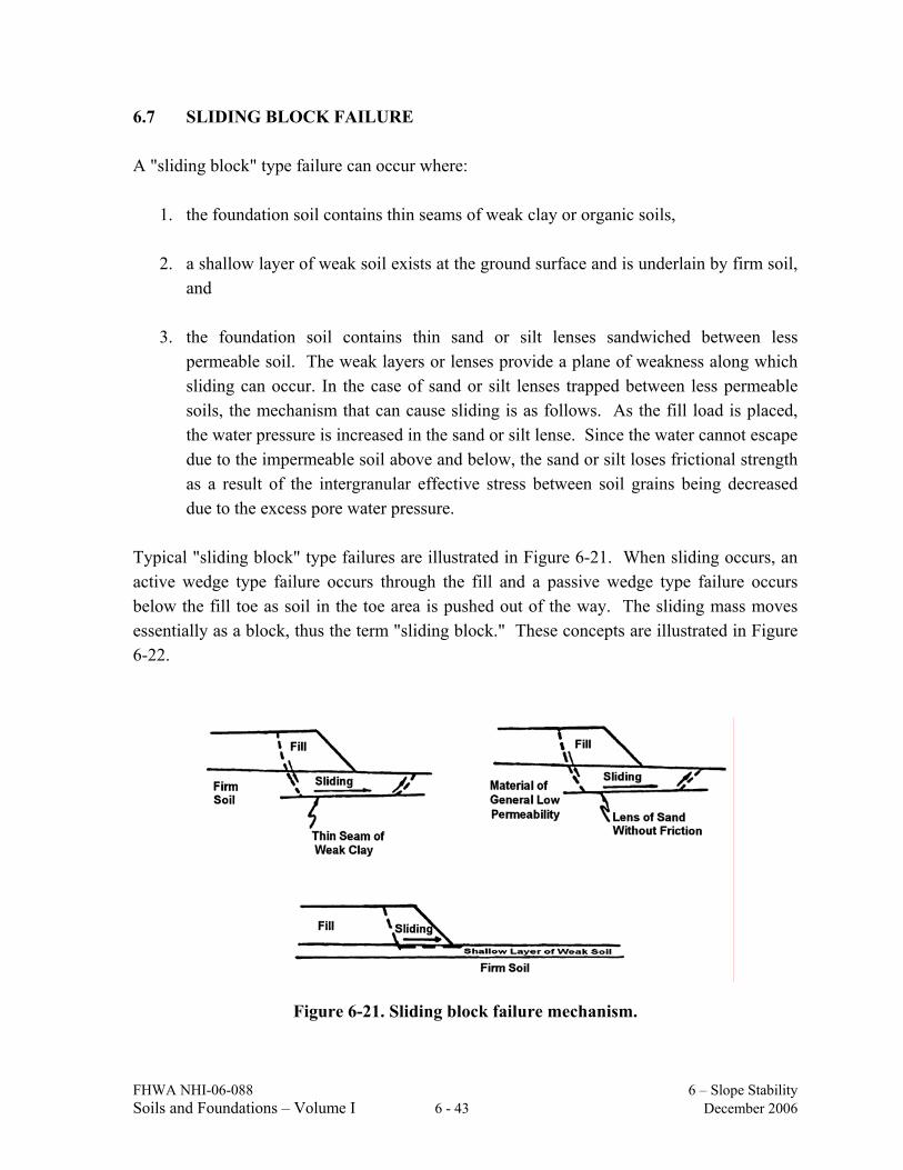
6.7 SLIDING BLOCK FAILURE A "sliding block" type failure can occur where:
1. the foundation soil contains thin seams of weak clay or organic soils,
2. a shallow layer of weak soil exists at the ground surface and is underlain by firm soil, and
3. the foundation soil contains thin sand or silt lenses sandwiched between less
permeable soil. The weak layers or lenses provide a plane of weakness along which sliding can occur. In the case of sand or silt lenses trapped between less permeable soils, the mechanism that can cause sliding is as follows. As the fill load is placed, the water pressure is increased in the sand or silt lense. Since the water cannot escape due to the impermeable soil above and below, the sand or silt loses frictional strength as a result of the intergranular effective stress between soil grains being decreased due to the excess pore water pressure.
Typical "sliding block" type failures are illustrated in Figure 6-21. When sliding occurs, an active wedge type failure occurs through the fill and a passive wedge type failure occurs below the fill toe as soil in the toe area is pushed out of the way. The sliding mass moves essentially as a block, thus the term "sliding block." These concepts are illustrated in Figure 6-22.
Figure 6-21. Sliding block failure mechanism.
FHWA NHI-06-088 6 – Slope Stability Soils and Foundations – Volume I 6 - 44 December 2006
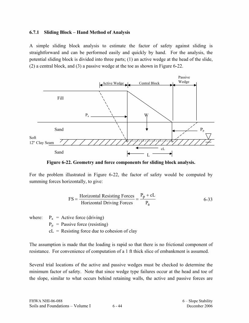
6.7.1 Sliding Block – Hand Method of Analysis A simple sliding block analysis to estimate the factor of safety against sliding is straightforward and can be performed easily and quickly by hand. For the analysis, the potential sliding block is divided into three parts; (1) an active wedge at the head of the slide, (2) a central block, and (3) a passive wedge at the toe as shown in Figure 6-22.
Figure 6-22. Geometry and force components for sliding block analysis. For the problem illustrated in Figure 6-22, the factor of safety would be computed by summing forces horizontally, to give:
a
pP
cLPForcesDrivingHorizontalForcesResistingHorizontalFS
+== 6-33
where: Pa = Active force (driving) Pp = Passive force (resisting) cL = Resisting force due to cohesion of clay The assumption is made that the loading is rapid so that there is no frictional component of resistance. For convenience of computation of a 1 ft thick slice of embankment is assumed. Several trial locations of the active and passive wedges must be checked to determine the minimum factor of safety. Note that since wedge type failures occur at the head and toe of the slope, similar to what occurs behind retaining walls, the active and passive forces are
Passive Wedge Central Block Active Wedge
W
Soft 12″ Clay Seam
Pa
cL
Pp
Fill
Sand
Sand L
FHWA NHI-06-088 6 – Slope Stability Soils and Foundations – Volume I 6 - 45 December 2006
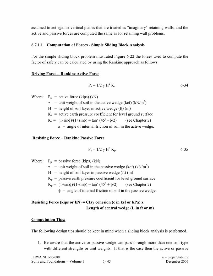
assumed to act against vertical planes that are treated as "imaginary" retaining walls, and the active and passive forces are computed the same as for retaining wall problems. 6.7.1.1 Computation of Forces - Simple Sliding Block Analysis For the simple sliding block problem illustrated Figure 6-22 the forces used to compute the factor of safety can be calculated by using the Rankine approach as follows: Driving Force – Rankine Active Force
Pa = 1/2 γ H2 Ka 6-34 Where: Pa = active force (kips) (kN) γ = unit weight of soil in the active wedge (kcf) (kN/m3) H = height of soil layer in active wedge (ft) (m)
Ka = active earth pressure coefficient for level ground surface Ka = (1-sinφ)/(1+sinφ) = tan2 (45o - φ/2) (see Chapter 2)
φ = angle of internal friction of soil in the active wedge. Resisting Force – Rankine Passive Force
Pp = 1/2 γ H2 Kp 6-35 Where: Pp = passive force (kips) (kN) γ = unit weight of soil in the passive wedge (kcf) (kN/m3) H = height of soil layer in passive wedge (ft) (m)
Kp = passive earth pressure coefficient for level ground surface Kp = (1+sinφ)/(1-sinφ) = tan2 (45o + φ/2) (see Chapter 2) φ = angle of internal friction of soil in the passive wedge.
Resisting Force (kips or kN) = Clay cohesion (c in ksf or kPa) x Length of central wedge (L in ft or m) Computation Tips: The following design tips should be kept in mind when a sliding block analysis is performed.
1. Be aware that the active or passive wedge can pass through more than one soil type with different strengths or unit weights. If that is the case then the active or passive

FHWA NHI-06-088 6 – Slope Stability Soils and Foundations – Volume I 6 - 46 December 2006
pressure distribution changes at the boundary between the different soils. This abrupt change in pressure is due to a change in either the angle of internal friction that affects the value of the earth pressure coefficient Ka or Kp and/or a change in the unit weight of the soil. The easiest way to handle this condition is to compute the active or passive earth pressure distribution diagram for each soil. There may be a discontinuity in the pressure diagram at the boundary between the two different soil layers. Then compute the active or passive force for each segment of the pressure distribution diagram from the area of each segment.
2. When the active or passive pressure is being computed for soils below the ground
water table, the buoyant (effective) unit weight of the soil must be used. The step-by step procedure for the Sliding Block Method of Analysis is illustrated by the following numerical example. Example 6-3: Find the safety factor for the 20 ft high embankment illustrated in Figure 6-23
by using the simple sliding block method and Rankine earth pressure coefficients. Consider a 1 ft wide strip of the embankment into the plane of the paper.
Figure 6-23. Example simple sliding block method using Rankine pressure coefficients.
Solution Step 1: Compute driving force, Pa, by using Equation 6-34 • Active Driving Force (Pa) by using Equation 6-34
1′
10′
Firm Material
Soft Clay Layer c = 400 psf
20′
2
1
γt = 110 pcf φ = 30°
γt = 110 pcf φ = 30°
FHWA NHI-06-088 6 – Slope Stability Soils and Foundations – Volume I 6 - 47 December 2006
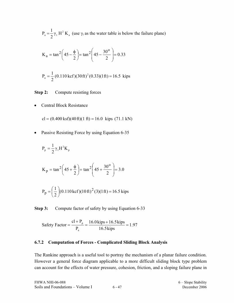
a2
ta KHγ21P = (use γt as the water table is below the failure plane)
33.02
3045tan2
45tanKo
22a =⎟
⎟⎠
⎞⎜⎜⎝
⎛−=⎟
⎠⎞
⎜⎝⎛ φ
−=
kips5.16)ft1)(33.0()ft30)(kcf110.0(21P 2
a ==
Step 2: Compute resisting forces • Central Block Resistance
kips16.0ft)ft)(1ksf)(40(0.400cl == (71.1 kN)
• Passive Resisting Force by using Equation 6-35
p2
tp KHγ21P =
0.32
3045tan2
45tanKo
22p =⎟
⎟⎠
⎞⎜⎜⎝
⎛+=⎟
⎠⎞
⎜⎝⎛ φ
+=
kips5.16)ft1)(3()ft10)(kcf110.0(21P 2
p =⎟⎠⎞
⎜⎝⎛=
Step 3: Compute factor of safety by using Equation 6-33
97.1kips5.16
kips5.16kips0.16P
PclFactorSafety
a
p =+
=+
=
6.7.2 Computation of Forces - Complicated Sliding Block Analysis The Rankine approach is a useful tool to portray the mechanism of a planar failure condition. However a general force diagram applicable to a more difficult sliding block type problem can account for the effects of water pressure, cohesion, friction, and a sloping failure plane in
FHWA NHI-06-088 6 – Slope Stability Soils and Foundations – Volume I 6 - 48 December 2006
the analysis. This analysis procedure, which is described in FHWA (2001a), can be used both to estimate the factor of safety for assumed failure surfaces in design or to "back-analyze" sliding block landslide problems. Computer solutions are also available for failure modes defined by planar and non-circular surfaces. However most of those solutions do not use the simplified Rankine block approach but rather a more complex failure plane such as that used in Janbu’s method. In general a computer solution is preferred for these planar failure problems because of the flexibility they offer in handling a variety of conditions that result in a more complex failure plane. 6.8 SLOPE STABILITY ANALYSIS USING COMPUTER PROGRAMS Slope stability procedures are well suited to computer analysis due to the interactive nature of the solution. Also, the simplified hand solution procedures do not properly account for interslice forces, irregular failure surfaces, seismic forces, and external loads such as line load surcharges or tieback forces. Several user-friendly computer programs exist to analyze two-dimensional slope stability problems. One of the advantages of a computer program is that it allows parametric studies to be performed by varying parameters of interest, e.g., shear strength parameters. More complex computer programs are available for three dimensional slope stability analysis. As a minimum, a basic two-dimensional slope stability program is recommended for routine use. Desirable geotechnical features of such a program should include:
• Multiple analysis capability a. Circular arc (Bishop) b. Non-circular (Janbu) c. Sliding block
• Variable input parameters to account for specific conditions a. Heterogeneous soil systems b. Pseudo-static seismic loads c. Ground anchor forces d Piezometric levels
• Random generation of multiple failure surfaces with an option to analyze a specific
failure surface.

FHWA NHI-06-088 6 – Slope Stability Soils and Foundations – Volume I 6 - 49 December 2006
Desirable software features include:
• User-friendly input screens including a summary screen that shows the cross section and soil boundaries in profile.
• Help screens and error tracking messages. • Expanded output options for both resisting forces in friction, cohesion or tieback
computations and driving forces in static or dynamic computations. • Ordered output and plotting capability for the failure surface of 10 minimum safety
factors. • Documentation of program.
A major problem for software users is technical support, maintenance and update of programs. Slope stability programs are in a continual process of improvement that can be expected to continue indefinitely. Highway agencies should implement only software that is documented and verified and for which the seller agrees to provide full technical support, maintenance and update. The following web page for the FHWA National Geotechnical Team contains links to distributors of FHWA software:
http://www.fhwa.dot.gov/engineering/geotech/index.cfm Similar services are provided for commercially available slope stability programs such as the ReSSA (2001), SLOPE/W, SLIDE, STABL series (e.g., PCSTABL, XSTABL, GSTABL), and UTEXAS. Appendix D provides an overview of use of the ReSSA program. Finally, it is extremely important for the designer to understand that the design is only as good as the input parameters. Therefore, the designer should put major emphasis where it belongs, which is on:
• Investigation • Sampling • Testing • Development of soil profile • Design soil strengths • Ground water table location
Computer programs are only tools that aid in the design. The answers are only as good as the input data. Don't get carried away with plugging in the numbers and examining the results. You may learn the "garbage in - garbage out" principle the hard way.
FHWA NHI-06-088 6 – Slope Stability Soils and Foundations – Volume I 6 - 50 December 2006
6.9 IMPROVING THE STABILITY OF EMBANKMENTS There are usually several technically feasible solutions to a stability problem. The chosen solution should be the most economical considering the following factors:
1. Available materials. 2. Quantity and cost of materials. 3. Construction time schedules. 4. Line and grade requirements. 5. Right-of-way issues.
6.9.1 Embankment Stability Design Solutions Table 6-2 presents a summary of practical solutions to mitigate embankment stability problems. Figures 6-24 to 6-26 illustrate some of the mitigation methods listed in Table 6-2. One of the solutions listed in Table 6-2 is the use of ground improvement. This solution can be used for cases where the internal stability of the embankment is not an issue due to the use of competent embankment materials, but the foundation materials are weak enough to affect the stability of the embankment slope. By improving the ground under the embankment, the resistance along the failure surface within the foundation is improved, thereby increasing the safety factor against slope failure. Relatively poor soils can be reinforced with geosynthetics to offset their low shear strength so that acceptable embankments can be constructed. Another solution is related to reinforcement of the embankment soils themselves. This solution can be used where the foundation is adequate but the locally available soils may not be suitable for construction of embankments at the desired slope angles. In this case, the embankment soils may be strengthened by the inclusion of reinforcements. Such slopes are called reinforced soil slopes (RSS). The RSS technology can be used to construct slopes at angles up to 69-degrees from horizontal. The RSS design method is discussed here as an example of a remediation method. Only the basics of the RSS design method are presented herein. Detailed design procedures for RSS technology can be found in FHWA (2001b). 6.9.2 Design Approach for Reinforced Soil Slopes The design of internal reinforcement for safe, steep slopes requires a rigorous analysis. The design of the reinforcement for this application is critical, as failure of the reinforcement would result in failure of the slope. The overall design requirements for reinforced slopes are similar to those for unreinforced slopes. The factor of safety must be adequate for both the short-term and long-term conditions and for all possible modes of failure.
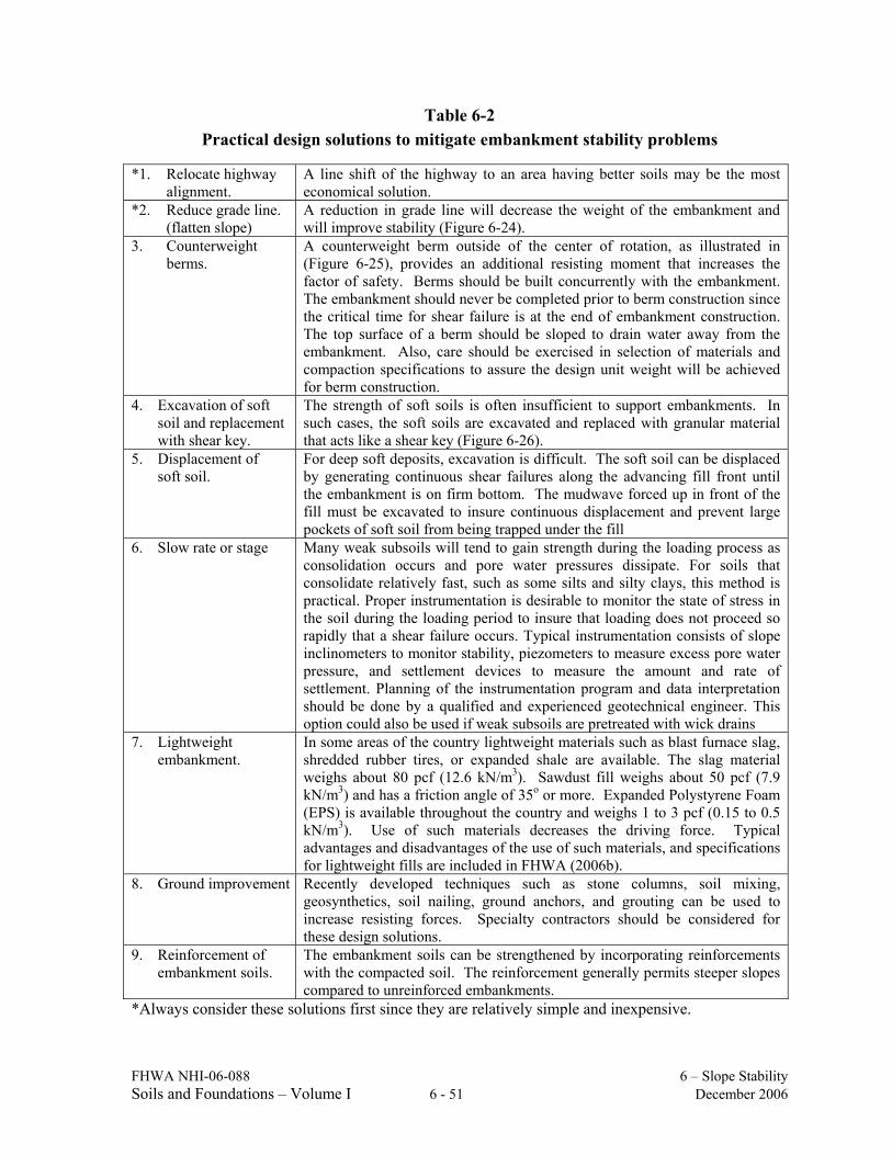
FHWA NHI-06-088 6 – Slope Stability Soils and Foundations – Volume I 6 - 51 December 2006
Table 6-2 Practical design solutions to mitigate embankment stability problems
*1. Relocate highway alignment.
A line shift of the highway to an area having better soils may be the most economical solution.
*2. Reduce grade line. (flatten slope)
A reduction in grade line will decrease the weight of the embankment and will improve stability (Figure 6-24).
3. Counterweight berms.
A counterweight berm outside of the center of rotation, as illustrated in (Figure 6-25), provides an additional resisting moment that increases the factor of safety. Berms should be built concurrently with the embankment. The embankment should never be completed prior to berm construction since the critical time for shear failure is at the end of embankment construction. The top surface of a berm should be sloped to drain water away from the embankment. Also, care should be exercised in selection of materials and compaction specifications to assure the design unit weight will be achieved for berm construction.
4. Excavation of soft soil and replacement with shear key.
The strength of soft soils is often insufficient to support embankments. In such cases, the soft soils are excavated and replaced with granular material that acts like a shear key (Figure 6-26).
5. Displacement of soft soil.
For deep soft deposits, excavation is difficult. The soft soil can be displaced by generating continuous shear failures along the advancing fill front until the embankment is on firm bottom. The mudwave forced up in front of the fill must be excavated to insure continuous displacement and prevent large pockets of soft soil from being trapped under the fill
6. Slow rate or stage Many weak subsoils will tend to gain strength during the loading process as consolidation occurs and pore water pressures dissipate. For soils that consolidate relatively fast, such as some silts and silty clays, this method is practical. Proper instrumentation is desirable to monitor the state of stress in the soil during the loading period to insure that loading does not proceed so rapidly that a shear failure occurs. Typical instrumentation consists of slope inclinometers to monitor stability, piezometers to measure excess pore water pressure, and settlement devices to measure the amount and rate of settlement. Planning of the instrumentation program and data interpretation should be done by a qualified and experienced geotechnical engineer. This option could also be used if weak subsoils are pretreated with wick drains
7. Lightweight embankment.
In some areas of the country lightweight materials such as blast furnace slag, shredded rubber tires, or expanded shale are available. The slag material weighs about 80 pcf (12.6 kN/m3). Sawdust fill weighs about 50 pcf (7.9 kN/m3) and has a friction angle of 35o or more. Expanded Polystyrene Foam (EPS) is available throughout the country and weighs 1 to 3 pcf (0.15 to 0.5 kN/m3). Use of such materials decreases the driving force. Typical advantages and disadvantages of the use of such materials, and specifications for lightweight fills are included in FHWA (2006b).
8. Ground improvement Recently developed techniques such as stone columns, soil mixing, geosynthetics, soil nailing, ground anchors, and grouting can be used to increase resisting forces. Specialty contractors should be considered for these design solutions.
9. Reinforcement of embankment soils.
The embankment soils can be strengthened by incorporating reinforcements with the compacted soil. The reinforcement generally permits steeper slopes compared to unreinforced embankments.
*Always consider these solutions first since they are relatively simple and inexpensive.
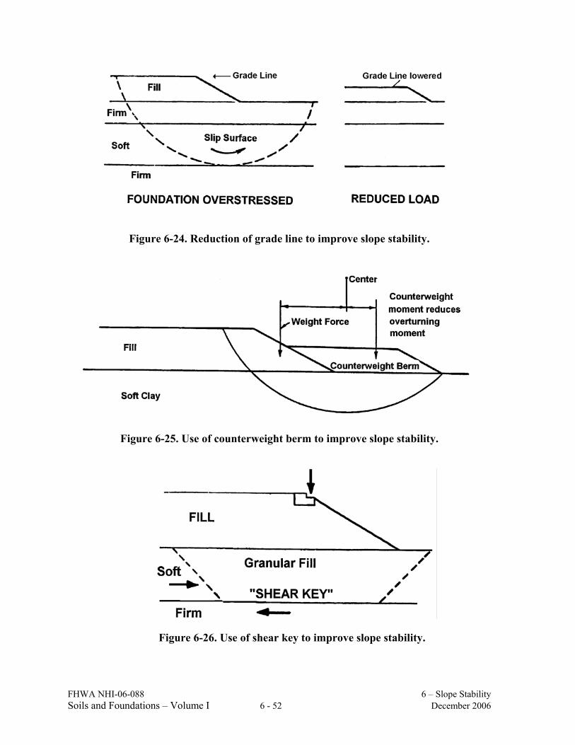
FHWA NHI-06-088 6 – Slope Stability Soils and Foundations – Volume I 6 - 52 December 2006
Figure 6-24. Reduction of grade line to improve slope stability.
Figure 6-25. Use of counterweight berm to improve slope stability.
Figure 6-26. Use of shear key to improve slope stability.
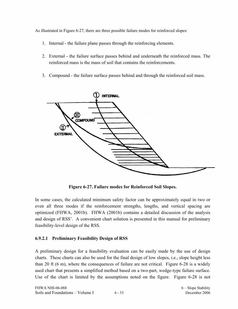
FHWA NHI-06-088 6 – Slope Stability Soils and Foundations – Volume I 6 - 53 December 2006
As illustrated in Figure 6-27, there are three possible failure modes for reinforced slopes:
1. Internal - the failure plane passes through the reinforcing elements.
2. External - the failure surface passes behind and underneath the reinforced mass. The reinforced mass is the mass of soil that contains the reinforcements.
3. Compound - the failure surface passes behind and through the reinforced soil mass.
Figure 6-27. Failure modes for Reinforced Soil Slopes. In some cases, the calculated minimum safety factor can be approximately equal in two or even all three modes if the reinforcement strengths, lengths, and vertical spacing are optimized (FHWA, 2001b). FHWA (2001b) contains a detailed discussion of the analysis and design of RSS’. A convenient chart solution is presented in this manual for preliminary feasibility-level design of the RSS. 6.9.2.1 Preliminary Feasibility Design of RSS A preliminary design for a feasibility evaluation can be easily made by the use of design charts. These charts can also be used for the final design of low slopes, i.e., slope height less than 20 ft (6 m), where the consequences of failure are not critical. Figure 6-28 is a widely used chart that presents a simplified method based on a two-part, wedge-type failure surface. Use of the chart is limited by the assumptions noted on the figure. Figure 6-28 is not
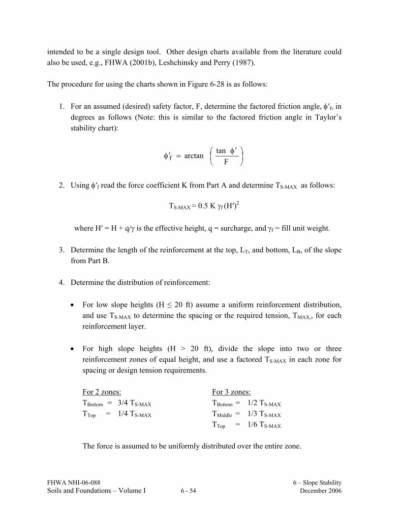
FHWA NHI-06-088 6 – Slope Stability Soils and Foundations – Volume I 6 - 54 December 2006
intended to be a single design tool. Other design charts available from the literature could also be used, e.g., FHWA (2001b), Leshchinsky and Perry (1987). The procedure for using the charts shown in Figure 6-28 is as follows:
1. For an assumed (desired) safety factor, F, determine the factored friction angle, φ′f, in
degrees as follows (Note: this is similar to the factored friction angle in Taylor’s stability chart):
⎟⎠⎞
⎜⎝⎛ φ ′
=φ′F
tanarctanf
2. Using φ′f read the force coefficient K from Part A and determine TS-MAX as follows:
TS-MAX = 0.5 K γf (H′)2
where H′ = H + q/γ is the effective height, q = surcharge, and γf = fill unit weight.
3. Determine the length of the reinforcement at the top, LT, and bottom, LB, of the slope
from Part B. 4. Determine the distribution of reinforcement:
• For low slope heights (H ≤ 20 ft) assume a uniform reinforcement distribution,
and use TS-MAX to determine the spacing or the required tension, TMAX,, for each reinforcement layer.
• For high slope heights (H > 20 ft), divide the slope into two or three
reinforcement zones of equal height, and use a factored TS-MAX in each zone for spacing or design tension requirements.
For 2 zones: For 3 zones: TBottom = 3/4 TS-MAX TBottom = 1/2 TS-MAX TTop = 1/4 TS-MAX TMiddle = 1/3 TS-MAX TTop = 1/6 TS-MAX The force is assumed to be uniformly distributed over the entire zone.
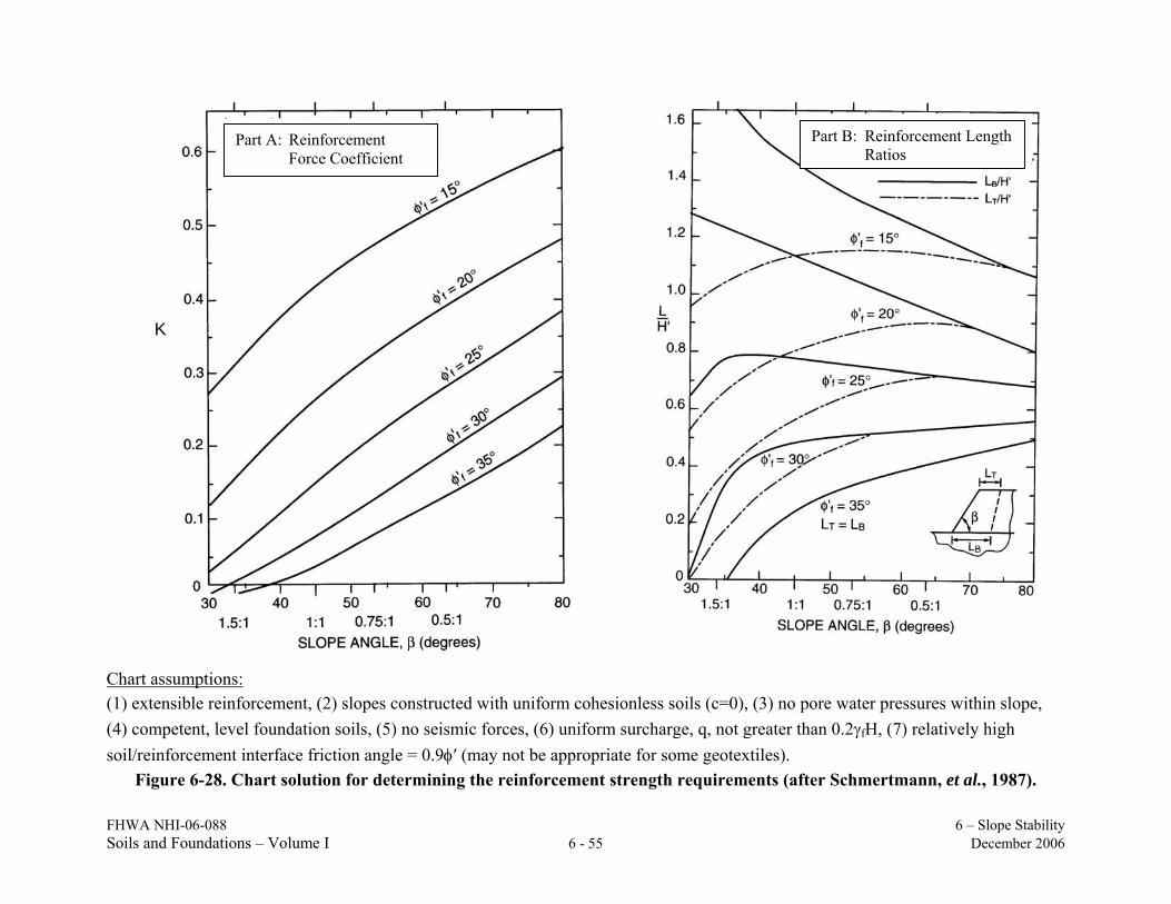
FHWA NHI-06-088 6 – Slope Stability Soils and Foundations – Volume I 6 - 55 December 2006
Chart assumptions: (1) extensible reinforcement, (2) slopes constructed with uniform cohesionless soils (c=0), (3) no pore water pressures within slope, (4) competent, level foundation soils, (5) no seismic forces, (6) uniform surcharge, q, not greater than 0.2γfH, (7) relatively high soil/reinforcement interface friction angle = 0.9φ′ (may not be appropriate for some geotextiles).
Figure 6-28. Chart solution for determining the reinforcement strength requirements (after Schmertmann, et al., 1987).
Part A: Reinforcement
Force Coefficient Part B: Reinforcement Length
Ratios
K
FHWA NHI-06-088 6 – Slope Stability Soils and Foundations – Volume I 6 - 56 December 2006
• Determine the requirements for vertical spacing of the reinforcement, Sv, or the maximum design tension, TMAX, for each reinforcement layer.
• For each zone, calculate TMAX for each reinforcing layer in that zone based on an
assumed Sv or, if the allowable reinforcement strength is known, calculate the minimum vertical spacing and number of reinforcing layers, N, required for each zone based on Equation 6-36 and the use of consistent units.
NT
HSTTRT zone
zone
vzonedca === 6-36
where: Ta = sum of available tensile force per width of reinforcement for all
reinforcement layers.
Rc = coverage ratio of the reinforcement that equals the width of the reinforcement, b, divided by the horizontal spacing Sh.
Sv = vertical spacing of reinforcement; multiples of compacted layer thickness for ease of construction.
Tzone = maximum reinforcement tension required for each zone. = TS-MAX for low slopes (H< 20 ft)
Hzone = height of zone. = Ttop, Tmiddle, and TBottom for high slopes (H > 20 ft)
N = number of reinforcement layers.
• In general, use short (4 - 6.5 ft (1.2 – 2 m)) lengths of reinforcement layers to maintain a maximum vertical spacing of 16 in (400 mm) or less for face stability and compaction quality. This short reinforcement should be placed in continuous layers and need not be as strong as the primary load bearing reinforcement, but it must be strong enough to survive construction (e.g., minimum survivability requirements for geotextiles in road stabilization applications in AASHTO M-288) and provide localized tensile reinforcement to the surficial soils.
For detailed analyses required for final design, refer to FHWA (2001b). The computer program ReSSA (2001) noted earlier, can perform analysis and design of reinforced soil slopes using the methods described in FHWA (2001b).

FHWA NHI-06-088 6 – Slope Stability Soils and Foundations – Volume I 6 - 57 December 2006
6.10 IMPROVING THE STABILITY OF CUT SLOPES The two most common types of cut slope failures are deep-seated and shallow surface failures. Both of these types of failure and their mitigation are discussed in this section. 6.10.1 Deep Seated Failure A deep seated failure usually occurs in slopes cut into clay. The clay has insufficient shear strength to support the slope, and shear failure generally occurs along a circular arc. If the clay contains water-bearing silt or sand layers, seepage forces will also contribute to the instability. Figure 6-29 shows an example of a deep seated failure and a possible design solution. Table 6-3 lists typical design solutions to potential cut slope stability problems in clay.
Figure 6-29. Deep seated slope failure (left) and bench slope design (right) to prevent slope failure.
Table 6-3
Typical design solutions to mitigate cut slope stability problems Design Solution Effect on Stability
a. Flatten slope. Reduces driving force.
b. Bench slope. Reduces driving force.
c. Buttress toe. Increases resisting force.
d. Lower water table. Reduces seepage force.
e. Reinforcement (e.g., nails) Increases resisting force The design of cut slopes in clay should NOT be based on the undrained strength of the clay determined by tests on samples obtained before the cut is made. Designs based on undrained strength will be unconservative since the effective stress is reduced when the cut is made because load is removed. This decrease in effective stress allows the clay to swell and
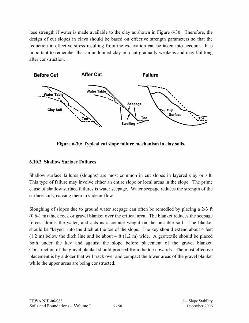
FHWA NHI-06-088 6 – Slope Stability Soils and Foundations – Volume I 6 - 58 December 2006
lose strength if water is made available to the clay as shown in Figure 6-30. Therefore, the design of cut slopes in clays should be based on effective strength parameters so that the reduction in effective stress resulting from the excavation can be taken into account. It is important to remember that an undrained clay in a cut gradually weakens and may fail long after construction.
Figure 6-30: Typical cut slope failure mechanism in clay soils.
6.10.2 Shallow Surface Failures Shallow surface failures (sloughs) are most common in cut slopes in layered clay or silt. This type of failure may involve either an entire slope or local areas in the slope. The prime cause of shallow surface failures is water seepage. Water seepage reduces the strength of the surface soils, causing them to slide or flow. Sloughing of slopes due to ground water seepage can often be remedied by placing a 2-3 ft (0.6-1 m) thick rock or gravel blanket over the critical area. The blanket reduces the seepage forces, drains the water, and acts as a counter-weight on the unstable soil. The blanket should be "keyed" into the ditch at the toe of the slope. The key should extend about 4 feet (1.2 m) below the ditch line and be about 4 ft (1.2 m) wide. A geotextile should be placed both under the key and against the slope before placement of the gravel blanket. Construction of the gravel blanket should proceed from the toe upwards. The most effective placement is by a dozer that will track over and compact the lower areas of the gravel blanket while the upper areas are being constructed.
FHWA NHI-06-088 6 – Slope Stability Soils and Foundations – Volume I 6 - 59 December 2006
6.10.3 Factor of Safety - Cut Slopes As indicated previously, a minimum design safety factor of 1.25 is used for routine highway embankment side slopes. A minimum factor of safety against sliding of 1.50 is recommended for the stability of cut slopes in fine-grained soils. The greater factor of safety for cut slopes is based upon the knowledge that cut slopes may deteriorate with time as a result of natural drainage conditions that embankments generally do not experience. In addition, there is a greater degree of uncertainty about the homogeneity of the soils in cut slopes than in embankment slopes that are engineered and constructed under controlled conditions.