geotechnical properties and foundation requirements for
TRANSCRIPT

Department of Civil Engineering – Stellenbosch University Page i
Geotechnical Properties and
Foundation Requirements for the
Satellite and Lunar Laser Ranger at the
Matjiesfontein Space Geodesy Observatory
by
Susan Bothma
Thesis presented in fulfilment of the requirements for the degree of
Master of Engineering in the Faculty of Civil Engineering at
Stellenbosch University
Supervisor: Mr Leon Croukamp
December 2015

Department of Civil Engineering – Stellenbosch University Page ii
DECLARATION
By submitting this thesis electronically, I declare that the entirety of the work contained therein is my
own, original work, that I am the sole author thereof (unless to the extent explicitly otherwise stated),
that reproduction and publication thereof by Stellenbosch University will not infringe any third party
rights and that I have not previously in its entirety or in part submitted it for obtaining any
qualification.
December 2015
Copyright © 2015 Stellenbosch University of Stellenbosch
All rights reserve
Stellenbosch University https://scholar.sun.ac.za

Department of Civil Engineering – Stellenbosch University Page iii
ABSTRACT
The basic idea of Satellite and Lunar Laser Ranging (S/LLR) is to improve our understanding of gravity.
The earth-moon system is a good workspace to test the theories of gravity. By measuring the distance
between the earth and the moon, the precise orbital shape of the path can be determined with
millimetre precision. This enables scientists to test general relativity (GR), which is the predicted
deviation from the Newtonian gravity and is supposed to exactly predict the correct orbital path of the
moon. With the measurements obtained from S/LLR experiments, scientists can compare the values to
those predicted by GR and this will help them to understand and prove the GR theorem.
The intention of this thesis is to identify, analyse and evaluate the required aspects for the emplacement
of an S/LLR at the Matjiesfontein Space Geodesy Observatory (MSGO). The 7 ton S/LLR needs a very
stable foundation to ensure accurate measurements as well as pointing to the exact location on the
satellite/lunar surface. The aspects evaluated is the bearing capacity of the rock mass, settlement of the
foundation, slope stability, excavatability of materials, the wind loads on the shed as well as the
management of risks. The following data is needed to complete the evaluation:
Field survey and tests:
o Geometric data capturing;
o Joint survey;
o DCP tests (Dynamic Cone Penetrometer); and
o Core Drilling.
Laboratory tests:
o UCS tests (Unconfined Compression Strength);
o Point load tests; and
o Petrographic analyses.
It was calculated that the applied bearing pressure is much smaller than the bearing capacity of the rock
and thus a safe assumption can be made that the rock mass is more than sufficient to withstand the load
of the structure.
From the result of the settlement calculation it is clear that settlement would not be a factor influencing
the operation of the S/LLR. It is recommended that the level of the foundation should be calibrated after
the hardening of the concrete and before the instrument is placed.
Slope stability analyses were done for potential circular failure, wedge failure, planar failure and
toppling. All of the slope stability analyses have shown that the areas are safe against slope instability
Stellenbosch University https://scholar.sun.ac.za

Department of Civil Engineering – Stellenbosch University Page iv
and no extra precautions need to be taken to keep the area safe. It is however important to do new
analyses if any cuts or excavations are made to build a road or building.
Bedrock can be found within 500 mm to 600 mm below ground level. The assessment of the
excavatability of materials yielded that the method of ripping should be used to excavate the material
on site. This indicates that the topsoil can be removed without the need for blasting to reach deep intact
rock.
Thin sections were prepared from the core samples and petrographic analyses were done to determine
the origin, composition, distribution and structure of the rocks. It is important to establish which clay
minerals are present to determine if the rock mass could be expansive and have a resultant
destabilising effect on the foundation. The petrographic studies have shown that clay minerals such as
kaolinite and chlorite are present in the samples. It can thus be concluded that, as these are non-
expansive minerals, it can be assumed to be a non-expansive rock mass.
The conclusion that can be drawn from this study is that the design of the foundations of the S/LLR at
MSGO will be the same as at HartRAO. This conclusion can be made as none of the factors that were
evaluated have shown a potential destabilising effect on the S/LLR.
Stellenbosch University https://scholar.sun.ac.za

Department of Civil Engineering – Stellenbosch University Page v
ACKNOWLEDGEMENTS
I would like to thank the following people:
Mr Leon Croukamp, for his guidance as my supervisor;
Dr Marius de Wet, for his support and guidance throughout the project;
Dr Stoffel Fourie, for his support and enabling me to visit the CERGA observatory in France;
Dr Ludwig Combrink, enabling me to visit HartRAO in Gauteng, South Africa;
Dr Peter Day, for his guidance and input towards my thesis;
Ms Danél van Tonder, for her assistance with the petrographic analyses;
Mr Jurgens Schoeman, for assisting with surveying and his knowledge of geological concepts;
Mr Jaco Pentz and Mr Lenmar Malan, for assisting with the surveying;
The laboratory assistants (geotechnical lab and structural lab), for their kind support; and
My parents and sister, for their support and understanding during the course of the project.
Stellenbosch University https://scholar.sun.ac.za

Department of Civil Engineering – Stellenbosch University Page vi
TABLE OF CONTENTS
Declaration .................................................................................................................................................................... ii
Abstract ......................................................................................................................................................................... iii
Acknowledgements .................................................................................................................................................... v
List of Figures ............................................................................................................................................................... ix
List of Tables .............................................................................................................................................................. xii
Chapter 1: Introduction ............................................................................................................................................ 1
1.1. Background ......................................................................................................................................................................... 1
1.2. Motivation for Research ................................................................................................................................................ 2
1.3. Research Purpose and Objectives ............................................................................................................................. 2
1.4. Limitations of Research ................................................................................................................................................. 2
1.5. The MSGO Site ................................................................................................................................................................... 2
1.5.1. Biophysical Attributes ....................................................................................................................................... 3
1.5.2. Geology .................................................................................................................................................................... 4
1.5.3. Weather Conditions ........................................................................................................................................... 4
1.5.4. Seismic Activity .................................................................................................................................................... 5
1.6. Report Layout and Structure ....................................................................................................................................... 5
Chapter 2: Literature Review .................................................................................................................................. 7
2.1. Lunar Laser Ranging ....................................................................................................................................................... 7
2.1.1. History of S/LLR .................................................................................................................................................. 7
2.1.2. How does the S/LLR work? ............................................................................................................................. 7
2.1.3. Other S/LLR Stations in the World ........................................................................................................... 11
2.1.4. The S/LLR at HartRAO ................................................................................................................................... 12
2.2. Geology .............................................................................................................................................................................. 15
2.2.1. The Cape Supergroup ..................................................................................................................................... 15
2.2.2. The Karoo Supergroup ................................................................................................................................... 17
2.2.3. Swelling Potential of a Rock Mass ............................................................................................................. 18
2.3. Previous Studies Done at MSGO .............................................................................................................................. 20
2.3.1. Research into the Foundation Requirements for a LLR at Matjiesfontein. .............................. 20
2.3.2. Palaeo-Landslides ............................................................................................................................................ 20
2.3.3. Slope Stability for Emplacement of Lunar Laser Ranger (LLR) .................................................... 21
Stellenbosch University https://scholar.sun.ac.za

Department of Civil Engineering – Stellenbosch University Page vii
2.3.4. Geotechnical Site Investigation .................................................................................................................. 21
2.3.5. EIA for Proposed MSGO ................................................................................................................................. 22
2.4. Slope Stability ................................................................................................................................................................. 22
2.4.1. Circular Slip ........................................................................................................................................................ 25
2.4.2. Planar Failure .................................................................................................................................................... 27
2.4.3. Wedge Failure .................................................................................................................................................... 29
2.4.4. Toppling ............................................................................................................................................................... 29
2.5. Foundation Types ......................................................................................................................................................... 30
2.5.1 Shallow Foundations: Spread Footings .................................................................................................... 31
2.5.2. Shallow Foundations: Raft Footings ......................................................................................................... 31
2.5.3. Deep Foundations: Piles ................................................................................................................................ 32
Chapter 3: Data Collection ..................................................................................................................................... 33
3.1. Field Survey and Tests ................................................................................................................................................ 33
3.1.1. Geometric Data Capturing ............................................................................................................................ 33
3.1.2. Joint Survey......................................................................................................................................................... 33
3.1.3. Dynamic Cone Penetrometer Test ............................................................................................................ 34
3.1.4. Core Drilling ....................................................................................................................................................... 37
3.2. Laboratory Tests ........................................................................................................................................................... 39
3.2.1. Unconfined Compression Test .................................................................................................................... 39
3.2.2. Point Load Test ................................................................................................................................................. 41
3.2.3. Petrographic Analysis .................................................................................................................................... 44
Chapter 4: Analysis of Data and Evaluation of Site ....................................................................................... 46
4.1. Bearing Capacity ............................................................................................................................................................ 46
4.2. Settlement ........................................................................................................................................................................ 51
4.3. Slope Stability ................................................................................................................................................................. 52
4.3.1. GeoSlope – SLOPE/W ..................................................................................................................................... 52
4.3.2. Prokon - Geotechnical .................................................................................................................................... 56
4.4. Excavatability of Material .......................................................................................................................................... 57
4.5. Wind Loads ...................................................................................................................................................................... 58
4.6. Risk Management .......................................................................................................................................................... 60
Stellenbosch University https://scholar.sun.ac.za

Department of Civil Engineering – Stellenbosch University Page viii
Chapter 5: Conclusion and Recommendations .............................................................................................. 63
5.1. Bearing Capacity ............................................................................................................................................................ 63
5.2. Settlement ........................................................................................................................................................................ 63
5.3. Slope Stability ................................................................................................................................................................. 63
5.4. Excavatability of Material .......................................................................................................................................... 64
5.5. Wind Loads ...................................................................................................................................................................... 64
5.6. Final Remarks ................................................................................................................................................................. 64
Bibliography ............................................................................................................................................................... 66
Appendix A: As-Built Drawings ........................................................................................................................... 71
Appendix B: Construction Site Photos .............................................................................................................. 74
Appendix C: UCS Test Samples ............................................................................................................................. 77
Appendix D: Point Load Test Samples .............................................................................................................. 78
Appendix E: Petrographic Analyses ................................................................................................................... 80
Appendix F: RMR Calculations ............................................................................................................................. 92
Appendix G: Settlement Calculations ................................................................................................................ 95
Appendix H: Circular Failure ................................................................................................................................ 96
Appendix I: Planar Failure .................................................................................................................................. 105
Appendix J: DN - Values ........................................................................................................................................ 113
Stellenbosch University https://scholar.sun.ac.za

Department of Civil Engineering – Stellenbosch University Page ix
LIST OF FIGURES
Figure 1: Map of the Western Cape (Anonymous, 2015) ................................................................................................. 1
Figure 2: Site Layout of the Matjiesfontein Space Geodesy Observatory .................................................................. 3
Figure 3: Climate Chart of Sutherland (Anonymous, 2014) ............................................................................................ 4
Figure 4: Seismic Hazard Map of South Africa (Kijko et al., 2003) ............................................................................... 5
Figure 5: A Schematic Diagram of a Typical S/LLR System (Short, 2005) ................................................................ 8
Figure 6: Laser Table ....................................................................................................................................................................... 9
Figure 7: Difference Between Retroreflector and a Reflective Surface ...................................................................... 9
Figure 8: The Apollo 14 Retroreflector on the Moon (Jones & Glover, 2013) ...................................................... 10
Figure 9: Simplified Drawing of the Foundation of the S/LLR at HartRAO ........................................................... 13
Figure 10: Runoff Shed with Tracks ....................................................................................................................................... 13
Figure 11: Detailed Drawing of the Base and Tracks ...................................................................................................... 14
Figure 12: S/LLR Site Layout .................................................................................................................................................... 14
Figure 13: Location of the Cape Supergroup Rocks (Brink, 1981) ........................................................................... 16
Figure 14: Location and Distribution of the Karoo Basin in South Africa (Johnson et al., 2006) ................. 17
Figure 15: Structure of Clays (Lory, [S.a.]) .......................................................................................................................... 18
Figure 16: Classification of Slope Processes (Anonymous, 2013)............................................................................... 23
Figure 17: Four Basic Types of Failure (a) Circular Slip, (b) Planar Failure, (c) Wedge Slip and
(d) Toppling (Hoek & Bray, 1981) .................................................................................................................... 24
Figure 18: Shape of Circular Slips (Google Images) ........................................................................................................ 25
Figure 19: Stability Analysis With The Method of Slices (Craig, 2004) ................................................................... 26
Figure 20: Kinematic Analysis of Plane Sliding ................................................................................................................. 27
Figure 21: Block Sliding Down an Inclined Plane (Hunt, 2005) ................................................................................. 28
Figure 22: Definition of Geometrical Terms (Google Image) ...................................................................................... 30
Figure 23: Graphical Presentation of Wedge Failure (Hoek & Bray, 1981) .......................................................... 30
Figure 24: Different Types of Foundations (Day, 2014) ................................................................................................ 31
Figure 25: Stereonet from Software....................................................................................................................................... 34
Figure 26: Components of the DCP ......................................................................................................................................... 35
Figure 27: (a) Core Drilling Machine, (b) Core Sample and (c) Core Samples in Core Box ............................. 37
Figure 28: (a) Sample in UCS Testing Machine and (b) Sample After Failure ...................................................... 40
Figure 29: Specimen Shape Requirements for (a) the Diametral Test, (b) the Axial Test, (c) the Block
Test, and (d) the Irregular Lump Test (Ulusay and Hudson, 2006) .................................................... 41
Figure 30: (a) Point Load Test Machine, (b) sample in Point Load Test Machine and (c), (d) and (e)
Shows Samples After Failure............................................................................................................................... 43
Stellenbosch University https://scholar.sun.ac.za

Department of Civil Engineering – Stellenbosch University Page x
Figure 31: Photomicrographs of a Thin Section Showing Well Developed Bedding and Sorting on a
Microscale ................................................................................................................................................................... 45
Figure 32: Photomicrographs of a Thin Section Showing Straining in a Quartz Lense .................................... 45
Figure 33: 3D Model of Area Adjacent to S/LLR ............................................................................................................... 53
Figure 34: Images Created by SLOPE/W with (a) Cross-Section 1, (b) Cross-Section 2 and
(c) Cross-Section 2 without Protrusion. ......................................................................................................... 55
Figure 35: DN Values versus Depth ........................................................................................................................................ 57
Figure 36: Method Selection (Franklin, 1971) .................................................................................................................. 58
Figure 37: Wind Pressure on the Runoff Shed ................................................................................................................... 60
Figure 38: Risk Management .................................................................................................................................................... 60
Figure 39: Construction of the S/LLR Foundation at HartRAO: Tracks .................................................................. 74
Figure 40: Construction of the S/LLR Foundation at HartRAO: Base ...................................................................... 74
Figure 41: Construction of the S/LLR Foundation at HartRAO: Completed .......................................................... 75
Figure 42: Placing of the S/LLR on the Base of the Foundation ................................................................................. 75
Figure 43: The S/LLR at HartRAO, with Run-Off Shed in Background .................................................................... 76
Figure 44: Samples After UCS Testing. (a) Sample 1C, (b) Sample 2C, (c) Sample 2D and
(d) Sample 2E. ........................................................................................................................................................... 77
Figure 45: Samples After Point Load Testing. (a) Sample 1D, (b) Sample 1E, (c) Sample 2G and
(d) Sample 2F............................................................................................................................................................. 78
Figure 46: Samples After Point Load Testing. (a) Sample 3C, (b) Sample 3D, (c) Sample 3E and
(d) Sample 3F............................................................................................................................................................. 79
Figure 47: Photomicrographs of a Thin Section Showing Angular to Sub-Angular Quartz in a Clay-Mica
Matrix ............................................................................................................................................................................ 81
Figure 48: Photomicrographs of a Thin Section Showing Angular to Sub-Angular Quartz in a Clay-Mica
Matrix of Matrix Supported Layers .................................................................................................................. 81
Figure 49: Photomicrographs of a Thin Section Showing Angular to Sub-Angular Quartz in a Clay-Mica
Matrix. Note Some Straining in Quartz ........................................................................................................... 82
Figure 50: Photomicrographs of a Thin Section Showing Angular to Sub-Angular Quartz in a Clay-Mica
Matrix ............................................................................................................................................................................ 84
Figure 51: Photomicrographs of a Thin Section Showing Angular to Sub-Angular Quartz in a Clay-Mica
Matrix ............................................................................................................................................................................ 84
Figure 52: Photomicrographs of a Thin Section Showing Angular to Sub-Angular Quartz in a Clay-Mica
Matrix. Note Dark and Light Rithmic Layering ............................................................................................ 86
Figure 53: Photomicrographs of a Thin Section Showing Angular to Sub-Angular Quartz in a Clay-Mica
Matrix. Close-Up View of Straining in Quartz and Clay-Minerals in the Matrix ............................. 86
Stellenbosch University https://scholar.sun.ac.za

Department of Civil Engineering – Stellenbosch University Page xi
Figure 54: Photomicrographs of a Thin Section Showing Unrounded to Angular Quartz in a Clay-Mica
Matrix ............................................................................................................................................................................ 88
Figure 55: Photomicrographs of a Thin Section Showing Angular to Sub-Angular Quartz in a Clay-Mica
Matrix ............................................................................................................................................................................ 90
Figure 56: Photomicrographs of a Thin Section Showing Angular to Sub-Angular Quartz in a Clay-Mica
Matrix. Close-Up View of Quartz-Dominated Layer Showing Straining and Recrystallisationin
Quartz, Overgrowths and Clay-Mica Matrix as well as Iron Oxide Staining .................................... 90
Figure 57: Photomicrographs of a Thin Section Showing Angular to Sub-Angular Quartz in a Clay-Mica
Matrix. Showing Straining and Recrystallisationin Quartz, Overgrowths and Clay-Mica Matrix
as well as Iron Oxide Staining ............................................................................................................................. 91
Figure 58: Photomicrographs of a Thin Section Showing Angular to Sub-Angular Quartz in a Clay-Mica
Matrix. Note Some Straining in Quartz ........................................................................................................... 91
Figure 59: Section 1 for Circular Failure Analysis ............................................................................................................ 96
Figure 60: Slope 2 With Protrusion for Circular Failure Analysis ............................................................................. 99
Figure 61: Section 2 Without Protrusion for Circular Failure Analysis ............................................................... 102
Stellenbosch University https://scholar.sun.ac.za

Department of Civil Engineering – Stellenbosch University Page xii
LIST OF TABLES
Table 1: Geology of MSGO With Formations Ordered From Youngest (Top) to Oldest ................................... 15
Table 2: Composition of the Clay Minerals Showing Both Elements and Chemical Compounds
(Pettersen, 2014) ........................................................................................................................................................ 19
Table 3: Classification of Slope Processes (Mathewson, 1981) .................................................................................. 22
Table 4: Main Dip Directions ..................................................................................................................................................... 34
Table 5: Data from DCP Tests ................................................................................................................................................... 36
Table 6: Core Logging Sheet ...................................................................................................................................................... 38
Table 7: UCS Test Data ................................................................................................................................................................. 40
Table 8: Point Load Test Data ................................................................................................................................................... 43
Table 9: Aspects Considered for Evaluation ....................................................................................................................... 46
Table 10: Rock Mass Rating System (Bieniawski, 1989) ............................................................................................... 48
Table 11: RMR Data ...................................................................................................................................................................... 49
Table 12: Bearing Capacity Calculation Parameters ....................................................................................................... 49
Table 13: Settlement Calculation Parameters ................................................................................................................... 52
Table 14: Soil Properties (Visser 2012) ............................................................................................................................... 53
Table 15: Factors of Safety For Circular Slip ...................................................................................................................... 54
Table 16: Conventions Used in Prokon ................................................................................................................................. 56
Table 17: Factors of Safety for Planar Failure.................................................................................................................... 57
Table 18: Parameters used in Prokon Calculation ........................................................................................................... 59
Table 19: Risk Assessment Matrix .......................................................................................................................................... 61
Table 20: Risk Register ................................................................................................................................................................ 62
Stellenbosch University https://scholar.sun.ac.za

Department of Civil Engineering – Stellenbosch University Page 1
CHAPTER 1: INTRODUCTION
1.1. BACKGROUND
Matjiesfontein is situated ±250 km Northeast from Cape Town via the N1 on the way to Laingsburg in
the Great Karoo, Western Cape. Figure 1 shows where Matjiesfontein is situated in the Western Cape.
The town dates back to 1884, when James Logan bought the farm. He then turned it into a luxurious spa
that was known far and wide (Anonymous, 2010).
FIGURE 1: MAP OF THE WESTERN CAPE (ANONYMOUS, 2015)
Although it was a very small town, Matjiesfontein lacked nothing. It had the longest private phone line,
its main street was lit by London street lamps, and it was the first village in South Africa to replace gas
with electricity. Matjiesfontein’s history also includes the first cricket match played between South
Africa and England, Olive Schreiner’s residency, controversial war crime hearings and accommodated
the Cape Command headquarters during the Anglo-Boer War.
Matjiesfontein
Stellenbosch University https://scholar.sun.ac.za

Department of Civil Engineering – Stellenbosch University Page 2
1.2. MOTIVATION FOR RESEARCH
The donation of a 1 m Cassegrain telescope by France to HartRAO (Hartebeesthoek Radio Astronomy
Observatory) created the opportunity to develop the Matjiesfontein Space Geodesy Observatory
(MSGO). Instruments such as a Satellite and Lunar Laser Ranger (S/LLR), gravimeter, seismograph and
a Global Navigation Satellite Systems (GNSS) receiver will be part of this observatory. In addition to the
mentioned instruments, the site could be considered for the installation of one or two 34 m dishes as
part of the NASA Deep Space Tracking Network. These dishes may be suitable for International Celestial
Reference Framework VLBI (Very Long Baseline Interferometry) experiments. The possible future
installation of a DORIS (Doppler Orbitography and Radiopositioning Integrated by Satellite) system will
further enhance satellite tracking and orbit calculations.
As the S/LLR is one of the main instruments on site, it is of utmost importance to ensure that the
instrument is stable and safe. This thesis will investigate all aspects needed to endorse the
emplacement.
1.3. RESEARCH PURPOSE AND OBJECTIVES
The objective of this study is to ensure safe and stable emplacement of the S/LLR at the MSGO. To do
this, the geotechnical properties of the site need to be determined and various aspects need to be taken
into consideration. This includes aspects such as bearing capacity, settlement, slope stability,
excavatability of materials and wind loading. Another objective is to identify possible risks that may
occur before, during or after construction, and to define an action to mitigate these risks.
1.4. LIMITATIONS OF RESEARCH
The research was limited to the effect of static loads on the ground such as the weight of the foundation
and the weight of the telescope. The vibrations and movement of the telescope was not taken into
consideration. The study is furthermore limited to only those aspects deemed critical to determine the
stability of the foundation, and not all aspects and risks were taken into consideration.
1.5. THE MSGO SITE
The site, where all the instruments will be placed, is situated ± 5 km to the south of Matjiesfontein. This
site was proposed for the MSGO as an outstation for HartRAO. The location is ideal, because it is
situated in a small depression that shields it from radio frequency interference emitted by cell phones
and microwave sources (Combrinck, et al,. 2007). This site is also favourable due to the many cloudless
days and clear skies which allow the S/LLR to increase its data collection efficiency. Figure 2 shows the
site layout of the MSGO.
Stellenbosch University https://scholar.sun.ac.za

Department of Civil Engineering – Stellenbosch University Page 3
FIGURE 2: SITE LAYOUT OF THE MATJIESFONTEIN SPACE GEODESY OBSERVATORY
1.5.1. BIOPHYSICAL ATTRIBUTES
The topography of this site is generally flat, with a ridge to the northern border of the site and a steep
slope (the Witteberg Mountains) to the South. The soil is usually shallow on top of weathered or hard
rock. Following a geotechnical investigation of eight test pits, the general regolith profile of this area
could be described as:
0.2 m: Dry, light brown, loose, intact, boulders and gravel in a sandy matrix. Hill wash.
0.5 m: Slightly moist, dark reddish-orange, dense, intact, boulders and gravel with limited
sandy matrix. Hill wash.
0.6-1 m: Refusal on highly to moderate weathered thinly bedded shale or mudstone. Bedding
planes sub-vertical (Combrinck, et al., 2007).
The vegetation present in this area is Matjiesfontein Shale Renosterveld and Koedoesberge-
Moordenaars Succulent Karoo. None of the vegetation or species found in this area is classified as
threatened and critically endangered, and no vulnerable, threatened or critically endangered species
were found in this area (Ecosense, 2015). This area, however, falls in a Critical Biodiversity Area, but
has not been formalized into a bioregional plan. A number of drainage channels run through this area,
5km to
Matjiesfontein Proposed
site 2
for S/LLR
Proposed
site 1
for S/LLR
Proposed site for
Radio Telescope
Antennas
Vault
GPS
Stellenbosch University https://scholar.sun.ac.za

Department of Civil Engineering – Stellenbosch University Page 4
but no wetlands are present. There is an access road to the site which is in a poor condition and eroded
in some areas. Three non-operational boreholes are present on site with a water pipeline towards one,
but it is not connected.
1.5.2. GEOLOGY
The MSGO site lies within the Greater Karoo and is close to the contact point between the Cape and
Karoo Supergroups. This area has gone through many geological stages starting with the breakup of
Pangea and turning into a shallow inland sea, later to be covered by large glaciers and then becoming a
sea again. After millions of years it finally became as dry and open as it is today. The layers in this area
have twisted and folded over long periods of time as a direct result of formation of the Cape Fold Belt.
Formations found in this area include the Waaipoort, Floriskraal and Kweekvlei Formations from the
Witteberg Group in the Cape Supergroup and the Dwyka Formation and Group in the Karoo
Supergroup.
1.5.3. WEATHER CONDITIONS
Weather conditions play a major part in activating slope movement (Tarbuck, et al., 1996), thus it is
important to investigate weather patterns thoroughly. There are no available weather data for
Matjiesfontein, but Sutherland is assumed to have similar conditions, so it is considered suitable to use
the same data for Matjiesfontein.
The Karoo region has a semi-arid climate with the mean annual precipitation (MAP) less than 250 mm
(Combrinck, et al., 2007). Figure 3 shows climate data obtained of Sutherland.
FIGURE 3: CLIMATE CHART OF SUTHERLAND (ANONYMOUS, 2014)
Stellenbosch University https://scholar.sun.ac.za

Department of Civil Engineering – Stellenbosch University Page 5
1.5.4. SEISMIC ACTIVITY
South Africa is not generally known for large seismic events, but due to the fact that an activity can
cause slopes failure processes to activate, it needs to be investigated. A hazard map of South Africa,
Figure 4, was created by Kijko et al., (2003). Matjiesfontein lies in an orange region with a peak ground
acceleration (PGA) of 0.16 g. This value is used in calculations when slope stability is investigated.
FIGURE 4: SEISMIC HAZARD MAP OF SOUTH AFRICA (KIJKO ET AL., 2003)
1.6. REPORT LAYOUT AND STRUCTURE
This thesis consists of five chapters, which include an introduction, a literature review, data collection,
analysis of data and evaluation of site, and risk management, followed by conclusions and
recommendations. Each chapter will be described in short.
The literature review, in Chapter 2, starts with LLR and gives a brief history thereof, how it works and
other stations in the world. The geology of the site is described with attention paid to the Cape
Supergroup as well as the Karoo Supergroup. The swelling potential of a rock mass is discussed in
addition. Previous studies done at the MSGO are included and followed by the discussion of slope
Stellenbosch University https://scholar.sun.ac.za

Department of Civil Engineering – Stellenbosch University Page 6
stability. The next section discusses different types of foundations and the chapter ends off with the
description of the S/LLR at HartRAO.
The data collection chapter, Chapter 3, deals with all activities associated with collection of data on the
site, including fieldwork and testing. Field work consists of geometric data capturing, a joint survey,
dynamic cone penetrometer tests as well as core drilling. The laboratory tests conducted were the
unconfined compression test, the point load test and petrographic analyses.
The analysis of the data obtained as well as the evaluation thereof is in the fourth chapter. The aspects
evaluated are the bearing capacity of the rock mass, settlement of the foundation, slope stability,
excavatability of materials, the wind loads on the shed as well as the management of risks.
In the final chapter, Chapter 5, conclusions are drawn and appropriate recommendations are made. In
the appendices, the extended calculations can be found as mentioned in the text.
Stellenbosch University https://scholar.sun.ac.za

Department of Civil Engineering – Stellenbosch University Page 7
CHAPTER 2: LITERATURE REVIEW
This chapter will discuss the literature that was studied in order to understand the problem as stated in
Section 1.3. It includes the history of LLR, the geology of the site, previous studies done and different
types of foundations which are used in practice.
2.1. LUNAR LASER RANGING
In order to understand the concept of LLR, a brief history and breakdown of the main elements of LLR
need to be discussed. In conjunction herewith, other LLR stations in the world are discussed with
particular attention paid to the S/LLR at HartRAO.
2.1.1. HISTORY OF S/LLR
According to Alley (1972), in the 1950’s a small group of scientists, from Princeton University under
Robert H. Dicke, gave substance to the concept of what would become the technique of optical laser
ranging. The group wanted to investigate the fundamentals of gravity and suggested that a powerful,
pulsed search light should be aimed at a reflector on a satellite. This would enable them to analyse the
orbital characteristics of the satellite.
Parallel to this process the concept of receiving laser light rebounds from the lunar surface proceeded.
The rough topography of the moon caused light to disperse and thus impossible to determine the
distance as precise as the satellite measurements, which then lead to the need, development and
placement of retroreflector arrays. The first retroreflector array was placed on the moon on 22 July
1969 (Dickey, 1994) during the Apollo 11 mission by Neil Armstrong and Buzz Aldrin. The first lunar
laser ranging observation of Apollo 11 was done shortly thereafter. This event made the concept of
lunar laser ranging (LLR) a reality. During the Apollo 14 and Apollo 15 missions additional
retroreflectors were placed on the moon and unmanned Soviet rovers (Lunokhod 1 and Lunokhod 2)
carrying a French-built reflector was placed on the surface as well (Murphy, 2013). No return signals
were detected from Lunokhod 1 after 1971, but in April 2010 a team from University of California
rediscovered it with the use of lunar images from NASA.
2.1.2. HOW DOES THE S/LLR WORK?
The basic idea of LLR is to improve our understanding of gravity and the earth-moon system is a good
workspace to test the theories. By measuring the distance between the earth and the moon, the precise
orbital shape of the path can be determined with millimetre precision. This enables scientists to test
general relativity (GR), which is the predicted deviation from the Newtonian gravity and supposed to
Stellenbosch University https://scholar.sun.ac.za

Department of Civil Engineering – Stellenbosch University Page 8
exactly predict the correct path of the moon (Murphy, 2013). With the measurements obtained from the
LLR experiment, scientists can compare the values to those predicted by GR and this will help them
understand and prove the GR theorem.
SLR and LLR are very valuable techniques which can contribute to a wide variety of fields such as
geodynamics, geodesy, astronomy, lunar science, relativity and gravitational physics (Veillet et al.,
1993). To use the technique of laser ranging, various elements need to work together. First a laser pulse
needs to be created and sent through the transmitter to the exact location on the lunar surface or
satellite, secondly a reflector must reflect the pulse back to earth and lastly a receiver must be able to
detect these pulses, measure the time of flight and calculate the distance. Figure 5 shows a simple
illustration of these elements.
FIGURE 5: A SCHEMATIC DIAGRAM OF A TYPICAL S/LLR SYSTEM (SHORT, 2005)
SLR operation is very similar to LLR, with only a few differences which include the speed of the
telescope itself and different types of pulses. As a satellite is much lower or closer to Earth than the
moon, the telescope have to move much faster to track a satellite, but needs less energy per pulse to
reach it.
2.1.2.1. The Laser Pulse
The pulse that is transmitted needs to be created on a laser table similar to that in Figure 6. The pulse is
created by an excited atom that duplicates a passing photon into a photon of the same energy. This
cloning process where a photon passes through a bulk material of excited atoms creates an exponential
growth in the light intensity. This process takes place until the light intensity is high enough to be
released by the laser system. The process is called the process of Stimulated Emission (Botha, 2015).
Stellenbosch University https://scholar.sun.ac.za

Department of Civil Engineering – Stellenbosch University Page 9
Once the pulse leaves the laser system, it is reflected by mirrors through the coudé path, to the point
where it can be transmitted to either the reflector on the lunar surface or the satellite. Stations that do
both SLR and LLR usually have a mirror that can turn to allow different types of laser pulses from
different laser tables to be transmitted. This is very useful as it makes it possible to do various
measurements with one telescope.
FIGURE 6: LASER TABLE
2.1.2.2. The Retroreflectors
A retroreflector is an array of corner cube reflectors, such as used in surveying, which reflects the light
directly back to its source independently of the angle of the beam. This is unlike a reflective surface
such as a mirror where the light is reflected back at the same angle as it arrived, as seen in Figure 7. A
flat mirror will only reflect the beam directly back to its source if the beam strikes the surface at exactly
90 degrees. Figure 8 shows an example of the Apollo 14 reflector on the moon that is used in LLR.
FIGURE 7: DIFFERENCE BETWEEN RETROREFLECTOR AND A REFLECTIVE SURFACE
Stellenbosch University https://scholar.sun.ac.za

Department of Civil Engineering – Stellenbosch University Page 10
FIGURE 8: THE APOLLO 14 RETROREFLECTOR ON THE MOON (JONES & GLOVER, 2013)
2.1.2.3. The Receiver
The distance between the earth and the moon is measured by the time it takes for the light pulse to
travel to the moon and back. This can be anywhere from 2.34 to 2.71 seconds, depending on the
distance to the moon at that time, and can be measured to an accuracy of a few picoseconds (Murphy,
2013).
In a period of a few hours, when the moon is at its highest, measurements are taken from all the visible
reflectors. By doing this over a few months or even years, the shape of the moon’s orbit will be defined
to such precision that assumptions can be made about the working of gravity.
However, to make such highly accurate measurements, as much laser light as possible is needed on the
reflector. The light pulses sent out must be as parallel and non-diverging as possible (Murphy, 2013).
This is why a laser is suitable, both for the short pulses of light it can give, and that a laser’s light is
highly directional. Due to the turbulent atmosphere of the Earth, the beam can be distorted up to 1.8 km
at the surface of the moon, which is very large considering that the reflector array is only 1 m2 and
means that most of the light will not reach its intended target. The width of the beam is about 15 km
across when it reaches the earth, which results in only 3 to 4 photon returns per minute (Murphy,
2013).
The light detector is the instrument that receives the photons in order to calculate the time. The
detector must also be orientated to the same location as the laser. The detector is programmed to
accept only the photons that were sent out by its system. This is possible because each photon is ‘time
stamped’ as it leaves the laser, the exact wavelength is known and the detector is only open for 100
nanoseconds when the photons are expected to return. They also incorporate an interferential filter
Stellenbosch University https://scholar.sun.ac.za
Department of Civil Engineering – Stellenbosch University Page 11
that only transmits light with that specific wavelength (Chapront & Francou, 1973). Laser ranging
cannot be done when it is full moon, as there would be too much background light and the detection of
the photons would be impossible.
The returning light from SLR and LLR differs. SLR returns a pulse of light which can be measured by a
Photo-Multiplier Tube (PMT). LLR returns only a single photon and a single-photon detection device is
used (typically an Avalanche Photo Detector (APD)).
A big uncertainty comes with the duration of a specific photon as it is impossible to know whether the
returning photon was at the beginning or at the end of the pulse that was emitted. The pulse can be
shortened with modern technology but this decreases the number of photons, and energy, which are
available to reach the moon (Veillet et al., 1993). A photon at the beginning of a pulse can differ as much
as 30 millimetres from the photon that is emitted last. A number of measurements are made over a
period of a few minutes and a statistical analysis can be made if 900 – 2500 photons are detected, to
improve the accuracy of 30 – 50 mm for one photon to 1 mm (Murphy, 2013).
There are a few elements to consider during the calculations. For accurate measurements the position
of the telescope relative to the centre of the earth should be known. This is, however, not a fixed
distance as the continental plate drifts and the tides from the moon and sun make the earth’s crust
expands whereas weather systems can also push the local crust down (Murphy, 2013). The
gravitational fields of other planets and celestial bodies can also have an effect (Combrinck, 2015). All of
these influences must be taken into consideration to determine the exact centre-to-centre distance
between the earth and the moon.
2.1.3. OTHER S/LLR STATIONS IN THE WORLD
After the reflectors were placed by Apollo 11, the first LLR observation was made by Lick Observatory
in California, for the purpose of quick acquisition and confirmation (Anonymous, 1993). Along with this,
LLR began at the McDonald Observatory and for 15 years the McDonald Observatory was the only
station that regularly ranged to the moon. Successful LLR was conducted in the early days by the
following observatories:
Air Force Cambridge Research Laboratories Lunar Ranging Observatory in Arizona;
Pic du Midi Observatory in France; and
Tokyo Astronomical Observatory.
Other stations that also accomplished lunar laser ranging in the past 40 years are Haleakala
Observatory on Maui Hawaii, the former Soviet Union, Australia and Germany. Currently there are only
a few operational LLR stations around the world, where most of the stations are shared SLR and LLR
Stellenbosch University https://scholar.sun.ac.za

Department of Civil Engineering – Stellenbosch University Page 12
stations (Dickey, 1994). The only stations to yield regular observations are the McDonald station in the
USA and the CERGA station in France.
McDonald Observatory is located near the community of Fort Davis in Jeff Davis County, Texas. The
observatory is situated in the Davis Mountains (west of Texas). There are two facilities in the
observatory, one on top of Mount Locke and the other on top of Mount Fowlkes.
McDonald Observatory was first approached by LURE (Lunar Ranging Experiment) when the 2.7 m
reflecting telescope became operational. This telescope was mostly funded by NASA for a major
planetary observation program. The operational telescope created the possibility for long-term LLR
activities at this site. McDonald Observatory became the leading LLR station in the world in the 1970’s
and early 1980’s (Silverberg, 1974)
The first LLR station in France was at Pic du Midi Observatory in the Pyrenees. A few echoes were
obtained from different reflectors, but it was difficult to sustain the operation as the site was isolated
and the team in charge of the experiment was situated in Paris. The team gained the necessary
experience and efforts were made for a dedicated LLR station (Veillet et al., 1993). The decision was
made to create a new observatory, CERGA (Centre d’Etudes et de Recherche en Géodynamique et
Astronomie), situated near Grasse, France. The observatory aimed to collect data (measurements in
astronomy) on the same site with several techniques, which includes astrolabes, a Schmidt telescope
and a SLR.
2.1.4. THE S/LLR AT HARTRAO
As discussed in Section 2.1.2., there is a difference in the pulse of SLR and LLR. The SLR at HartRAO has a
high rate of firing and low power with a frequency of 1 kilohertz, energy of 0.5 millijoule and a pulse
length of 20 picoseconds. The LLR has more power and thus more photons per pulse and a higher peak
pulse power with a frequency of 20 hertz, energy of 130 millijoule and a pulse length of 80 picoseconds
(Combrink, 2015).
The foundation of the S/LLR at HartRAO was designed by Endecon Ubuntu (Pty) Ltd Engineering
Consultants. Appendix A contains the as built drawing for the shed structure and foundation of the
S/LLR at HartRAO. As seen in Figure 9, the foundation consists of the base on which the S/LLR is
founded and 3 tracks for the runoff shed. Appendix B shows photos taken during the construction of
the S/LLR at HartroRAO.
Stellenbosch University https://scholar.sun.ac.za

Department of Civil Engineering – Stellenbosch University Page 13
FIGURE 9: SIMPLIFIED DRAWING OF THE FOUNDATION OF THE S/LLR AT HARTRAO
The S/LLR is protected by a runoff shed which opens during operation and closes afterwards. It takes
approximately 2 minutes and 30 seconds for the shed to open or close. This process is activated
manually. The shed runs on three IPE 180-beam tracks, as seen in Figure 10. The strip footings are
25 MPa reinforced concrete and 350 mm deep. The shed is constructed with steel segments, which can
be disassembled, resulting in easier transportation.
FIGURE 10: RUNOFF SHED WITH TRACKS
The base consists of a square ground floor which is underlain by two diagonal beams and a deep base at
each corner. Figure 11 shows a detailed drawing of the base and tracks, which is an extract from
Appendix A. All elements in the base are constructed from 30 MPa reinforced concrete. The ground
floor is 350 mm deep, the beams 600 mm deep and the corner bases 1200 mm deep.
Drawing not to scale
Stellenbosch University https://scholar.sun.ac.za

Department of Civil Engineering – Stellenbosch University Page 14
FIGURE 11: DETAILED DRAWING OF THE BASE AND TRACKS
Before ranging can take place, the S/LLR’s position needs to be calibrated and this is done with the use
of 5 levelling beacons. A beacon is a 0.7 m diameter, 2 m high, concrete pillar, with a corner cube
reflector on top. They are placed all around the S/LLR and are founded on bedrock to ensure stability.
The control room is situated next to the S/LLR, built in a temperature regulated container. The room
houses the laser table as well as the computers to control operation. The container is placed on the
ground, but the laser table’s foundation is independent. The legs of the table are drilled through the
floor of the container and stand on two I-beams, which are placed on the piers founded on bedrock.
Figure 12 shows the layout of the S/LLR covered by the shed as well as the control room.
FIGURE 12: S/LLR SITE LAYOUT
Stellenbosch University https://scholar.sun.ac.za
Department of Civil Engineering – Stellenbosch University Page 15
2.2. GEOLOGY
This section will describe the geology of the Cape- and Karoo- Supergroup with more attention paid to
the local geology. Formations found in the study area include the Waaipoort-, Floriskraal- and
Kweekvlei- Formations from the Witteberg Group in the Cape Supergroup and the Dwyka Formation
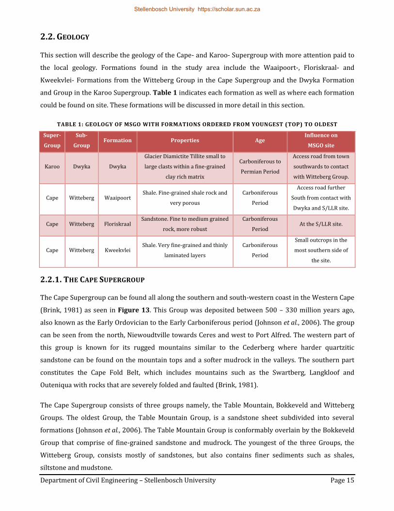
and Group in the Karoo Supergroup. Table 1 indicates each formation as well as where each formation
could be found on site. These formations will be discussed in more detail in this section.
TABLE 1: GEOLOGY OF MSGO WITH FORMATIONS ORDERED FROM YOUNGEST (TOP) TO OLDEST
Super-
Group
Sub-
Group Formation Properties Age
Influence on
MSGO site
Karoo Dwyka Dwyka
Glacier Diamictite Tillite small to
large clasts within a fine-grained
clay rich matrix
Carboniferous to
Permian Period
Access road from town
southwards to contact
with Witteberg Group.
Cape Witteberg Waaipoort Shale. Fine-grained shale rock and
very porous
Carboniferous
Period
Access road further
South from contact with
Dwyka and S/LLR site.
Cape Witteberg Floriskraal Sandstone. Fine to medium grained
rock, more robust
Carboniferous
Period At the S/LLR site.
Cape Witteberg Kweekvlei Shale. Very fine-grained and thinly
laminated layers
Carboniferous
Period
Small outcrops in the
most southern side of
the site.
2.2.1. THE CAPE SUPERGROUP
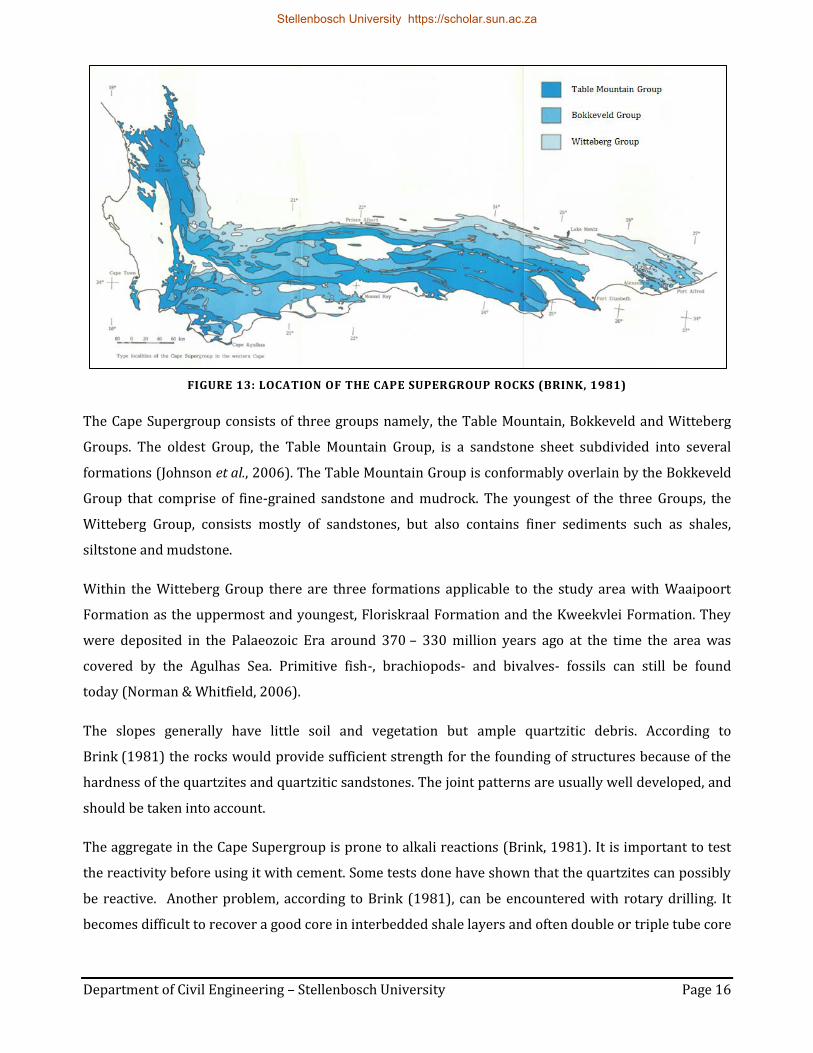
The Cape Supergroup can be found all along the southern and south-western coast in the Western Cape
(Brink, 1981) as seen in Figure 13. This Group was deposited between 500 – 330 million years ago,
also known as the Early Ordovician to the Early Carboniferous period (Johnson et al., 2006). The group
can be seen from the north, Niewoudtville towards Ceres and west to Port Alfred. The western part of
this group is known for its rugged mountains similar to the Cederberg where harder quartzitic
sandstone can be found on the mountain tops and a softer mudrock in the valleys. The southern part
constitutes the Cape Fold Belt, which includes mountains such as the Swartberg, Langkloof and
Outeniqua with rocks that are severely folded and faulted (Brink, 1981).
The Cape Supergroup consists of three groups namely, the Table Mountain, Bokkeveld and Witteberg
Groups. The oldest Group, the Table Mountain Group, is a sandstone sheet subdivided into several
formations (Johnson et al., 2006). The Table Mountain Group is conformably overlain by the Bokkeveld
Group that comprise of fine-grained sandstone and mudrock. The youngest of the three Groups, the
Witteberg Group, consists mostly of sandstones, but also contains finer sediments such as shales,
siltstone and mudstone.
Stellenbosch University https://scholar.sun.ac.za
Department of Civil Engineering – Stellenbosch University Page 16
FIGURE 13: LOCATION OF THE CAPE SUPERGROUP ROCKS (BRINK, 1981)
The Cape Supergroup consists of three groups namely, the Table Mountain, Bokkeveld and Witteberg
Groups. The oldest Group, the Table Mountain Group, is a sandstone sheet subdivided into several
formations (Johnson et al., 2006). The Table Mountain Group is conformably overlain by the Bokkeveld
Group that comprise of fine-grained sandstone and mudrock. The youngest of the three Groups, the
Witteberg Group, consists mostly of sandstones, but also contains finer sediments such as shales,
siltstone and mudstone.
Within the Witteberg Group there are three formations applicable to the study area with Waaipoort
Formation as the uppermost and youngest, Floriskraal Formation and the Kweekvlei Formation. They
were deposited in the Palaeozoic Era around 370 – 330 million years ago at the time the area was
covered by the Agulhas Sea. Primitive fish-, brachiopods- and bivalves- fossils can still be found
today (Norman & Whitfield, 2006).
The slopes generally have little soil and vegetation but ample quartzitic debris. According to
Brink (1981) the rocks would provide sufficient strength for the founding of structures because of the
hardness of the quartzites and quartzitic sandstones. The joint patterns are usually well developed, and
should be taken into account.
The aggregate in the Cape Supergroup is prone to alkali reactions (Brink, 1981). It is important to test
the reactivity before using it with cement. Some tests done have shown that the quartzites can possibly
be reactive. Another problem, according to Brink (1981), can be encountered with rotary drilling. It
becomes difficult to recover a good core in interbedded shale layers and often double or triple tube core
Stellenbosch University https://scholar.sun.ac.za

Department of Civil Engineering – Stellenbosch University Page 17
barrels are needed to ensure good recovery. The quartzites are quite difficult to drill through and thus
the drill rates are slow and time consuming.
2.2.2. THE KAROO SUPERGROUP
The Karoo Supergroup, the biggest basin in Southern Africa, as seen in Figure 14, was deposited
between 290 – 190 million years ago, also known as the late Carboniferous to the early Jurassic period
(Johnson et al., 2006). Radiometric dating showed that some parts of the basin continued to form up
until the separation of Africa and South America roughly 120 million years ago. This Supergroup
comprises of various rocks with a thickness of nearly 8 kilometres, including mudrock and sandstone,
tillite at the bottom, basalt as the top and coal about halfway up (Brink, 1983). The majority of the
strata are horizontal, but parts of the basin alongside the Cape Fold Belt have been folded under
pressure.
FIGURE 14: LOCATION AND DISTRIBUTION OF THE KAROO BASIN IN SOUTH AFRICA
(JOHNSON ET AL., 2006)
The basin consists of the Dwyka group, the Ecca Group, the Beaufort Group, the Drakensberg Group and
the Lebombo Group. These rocks include mudrock, sandstone, tillite, basalt, coal and dolerite
intrusions (Brink, 1983).
The oldest in the Karoo Supergroup and the youngest in the study area, the Dwyka Formation overlies
the Cape Supergroup unconformably in the South with various lithology types that have been
recognized (Johnson et al., 2006). The Dwyka Group is a diamicitite tillite formation, consisting of small
to large clasts within a fine-grained, clay rich matrix and in some areas, no clasts at all.
Stellenbosch University https://scholar.sun.ac.za

Department of Civil Engineering – Stellenbosch University Page 18
Sediment was fed by ice streams into the south-western part of the Karoo Basin. It was redistributed by
sediment gravity flows and turbidity currents. Together these deposits formed large subaqueous fans
that were controlled by the ice sheet dynamics (Visser et al., 2004).
2.2.3. SWELLING POTENTIAL OF A ROCK MASS
It is important to quantify the potential for swelling of a rock mass as it may have an adverse effect on
the stability of tunnels, slopes and foundations (Pettersen, 2014). To be able to determine the swelling
potential of a rock mass, a study of the clay minerals is needed. Most clay minerals have a basic
structural unit of a silicon-oxygen tetrahedron and an aluminium-hydroxyl octahedron (Craig, 2004).
These units combine to form different sheet structures as seen in Figure 15. Tetrahedral units combine
by the sharing of oxygen ions to form a silica sheet and the octahedral units combine by shared
hydroxyl ions to form a gibbsite sheet. The layers are formed by the bonding of a silica sheet with
either one or two gibbsite sheets. Stacks of these layers, with different bonding between them, make up
the clay minerals particles (Craig, 2004).
Clays, rich in montmorillonite (or smectite), may expand when it comes into contact with water, which
means that it has a swelling potential. The degree of expansion depends on the minerals present in the
clay. Clay minerals such as montmorillonite, vermiculite, illite or kaolinite can be expected and their
sensitivity to water varies. Montmorillonite is a highly expansive clay mineral, where vermiculite is
moderately expansive and illite or kaolinite non-expansive.
FIGURE 15: STRUCTURE OF CLAYS (LORY, [S.A.])
Stellenbosch University https://scholar.sun.ac.za

Department of Civil Engineering – Stellenbosch University Page 19
Two factors are needed to set this expansion into action, namely the internal factor, which is the ability
of the clay minerals to expand (chemical composition) and the external factor, the presence of water
(Pettersen, 2014). Exposed rock masses can be de- and resaturated which in turn result in swelling and
shrinkage and even fracturing (Zhang et al., 2010). Clay minerals present in the intact rock will not
result in expansion of the rock mass, but clay minerals present in the fractures and cracks may result in
expansion.
The chemical composition of clay minerals can be determined by the study of thin sections, also known
as petrographic analyses. This is the description and classification of rocks, but this optical
identification can be difficult when it is finely grained (Zhang et al., 2010). The better identification
method will be by means of x-ray examination.
There are two types of x-ray examination, X-Ray Diffraction (XRD) and X-Ray Fluorescence (XRF). XRD
can determine the presence and amounts of minerals species in a sample, as well as identify phases.
XRF will give details of the chemical composition of a sample but will not indicate what phases are
present in the sample. Table 2 shows the clay minerals and their corresponding elements and chemical
compounds.
TABLE 2: COMPOSITION OF THE CLAY MINERALS SHOWING BOTH ELEMENTS
AND CHEMICAL COMPOUNDS (PETTERSEN, 2014)
Montmorillonite:
Na0.2Ca0.1Al2Si4O10(OH)2(H2O)10
Vermiculite:
Mg1.8Fe2+0.9Al4.3SiO10(OH)2•4(H2O)
Element [%] Chemical
compound [%] Element [%]
Chemical compound
[%]
Sodium (Na) 0.84 Na2O 1.13 Magnesium (Mg) 8.68 MgO 14.39
Calcium (Ca) 0.73 CaO 1.02 Aluminium (Al) 23.01 Al2O3 43.48
Aluminium (Al) 9.83 Al2O3 18.57 Iron (Fe) 9.97 FeO 12.82
Silicon (Si) 20.46 SiO2 43.77 Silicon (Si) 5.57 SiO2 11.92
Hydrogen (H) 4.04 H2O 36.09 Hydrogen (H) 2 H2O 17.87
Oxygen (O) 64.11
Oxygen (O) 50.77
Illite:
K0.6(H3O)0.4Al1.3Mg0.3Fe2+0.1Si3.5O10(OH)2•(H2O)
Kaolinite:
Al2Si2O5(OH)4
Element [%] Chemical
compound [%] Element [%]
Chemical compound
[%]
Potassium (K) 6.03 K2O 7.26 Aluminium (Al) 20.9 Al2O3 39.5
Magnesium (Mg) 1.87 MgO 3.11 Silicon (Si) 21.76 SiO2 46.55
Aluminium (Al) 9.01 Al2O3 17.02 Hydrogen (H) 1.56 H2O 13.96
Iron (Fe) 1.43 FeO 1.85 Oxygen (O) 55.78
Silicon (Si) 25.25 SiO2 54.01
Hydrogen (H) 1.35 H2O 12.03
Oxygen (O) 55.06
Stellenbosch University https://scholar.sun.ac.za

Department of Civil Engineering – Stellenbosch University Page 20
2.3. PREVIOUS STUDIES DONE AT MSGO
There have been various studies done at Matjiesfontein. These studies include slope stability analyses,
preliminary designs for the low level water crossings, investigations and solutions for the eroded
surface of the access road, services to the site as well as rock mechanics for construction purposes. The
relevant topics discussed include foundation requirements for a LLR at MSGO, slope stability analyses, a
geotechnical site investigation and an EIA for the MSGO.
2.3.1. RESEARCH INTO THE FOUNDATION REQUIREMENTS FOR A LLR AT MATJIESFONTEIN.
This preliminary study focuses on the foundation requirements for the emplacement of the LLR. The
foundation will be responsible for the stable platform from where the LLR will operate (Croukamp
et al., 2011). The foundations should be built in such a way that it would cushion even minute
movement of the ground. It was suggested that the foundation of the LLR should be isolated from the
foundations of the auxiliary buildings as vibrations of footsteps is enough to induce detectable ground
movement.
The positions of the LLR need to be calibrated locally before any observations can be done. This will be
done by means of at least 4 beacons within about 300 m from the instrument. Each beacon will consist
of a circular column with a corner cube reflector on top. These beacons will be embedded into the
bedrock to minimize vertical and horizontal movement. Croukamp et al., (2011) found that the total
pressure which the foundation and the 7 ton LLR will exert on the rock mass is small compared to the
bearing capacity of the rock mass.
Since this study was conducted, the proposed site for the S/LLR has changed, resulting in new research
being required.
2.3.2. PALAEO-LANDSLIDES
Waters (2011) investigated palaeo-landslides at the MSGO. There was a need to determine whether the
site was safe for development as reactivation of the landslides can have a destabilizing effect on the
instruments on site.
The project included the surveying and mapping of two palaeo-landslides. The origin of the landslides
had to be determined to evaluate the possibility of reactivation of the slides, or new slides forming in
the region. The investigation included a joint survey, a slip-circle analysis, the potential for re-activation
of the landslides due to development and the possibility of rock toppling.
Various methods that were used in the assessment showed that slope-failure will not occur under the
investigated circumstances. All calculated safety factors were acceptable. Waters (2011), however,
Stellenbosch University https://scholar.sun.ac.za

Department of Civil Engineering – Stellenbosch University Page 21
suggested that the study could be improved by further testing and determining at what depth the
bedrock layer lies. He concluded that the development could continue as the slopes proved to be stable.
2.3.3. SLOPE STABILITY FOR EMPLACEMENT OF LUNAR LASER RANGER (LLR)
Visser (2012) investigated the slope stability of the area where the LLR was originally intended to be
placed. The study was done to determine whether the proposed site was suitable for this emplacement.
A new position for the S/LLR has since been identified, but data collected during the Visser study is still
valid.
Visser (2012) had done a GPS survey and created a 3D model. Various ways were identified in which
the slope was able to fail. On the southern side of the slope, planar failure and circular failure may occur
and on the northern side planar and wedge failure. It was concluded that the southern side of the slope
was stable, as the safety factors obtained were greater than 1.5. However, on the northern side of the
slope it was not stable or safe to cut more than 1 m, should an access road be constructed. Visser (2012)
concluded that, if no cuts are to be made on the northern side of the slope, the emplacement of the LLR
may continue.
2.3.4. GEOTECHNICAL SITE INVESTIGATION
A geotechnical site investigation was done at Matjiesfontein (Combrinck, et al., 2007), when it was
proposed for the new space geodetic observatory. The suitability of the location needed to be verified in
order to start with the project.
During the site investigation the following geophysical methods were used:
Magnetic Method;
Electromagnetic Method; and
Seismic Refraction Method.
Geotechnical investigation methods used included a walk-over site survey, digging of test pits and
description of the soil profile according to the MCCSSO system. After the investigation was completed,
the initial results showed that the site would be suitable for this project, but that further investigation
should be done around the foundations of each building. It was also recommended that the palaeo slope
failure, on the southern portion of the MSGO site and the northern slope of the Witteberg Mountains,
should not be disturbed.
Stellenbosch University https://scholar.sun.ac.za

Department of Civil Engineering – Stellenbosch University Page 22
2.3.5. EIA FOR PROPOSED MSGO
Ecosense Consulting Environmentalists cc was approached to do the screening report for the proposed
MSGO project. A basic assessment in terms of the National Environmental Management Act
Environmental Impact Assessment regulations would be required, because of the river crossings and
clearance of vegetation for access roads to the site. It was recommended by Ecosense (2010) that:
1. Alternative location for the emplacement of the instruments must be investigated.
2. An alternative to permanent river crossing structures (temporary structures) should be
investigated.
3. Current crossings should be repaired in such a way that it would avoid damming during flash
floods.
4. The EIA studies done for the road built by the municipality must be consulted for an operational
management plan.
2.4. SLOPE STABILITY
Failures are caused by the geometry of the slope and the type of materials combined with gravity, but is
frequently affected by water and water content of the materials. A general term used for all types of
failure is slope movement. Slope movement can be divided into five different types namely falls, topples,
slides, spreads and flows (Mathewson, 1981). Table 3 shows the classifications of the processes and
Figure 16 illustrates them.
TABLE 3: CLASSIFICATION OF SLOPE PROCESSES (MATHEWSON, 1981)
TYPE OF
MOVEMENT
TYPE OF MATERIAL
Rock Soil
Coarse Grain Fine Grain
Fall Rock Fall Debris Fall Earth Fall
Topple Rock Topple Debris Topple Earth Topple
Rotational Slide Rock Slump Debris Slump Earth Slump
Translational Rock Block Slide Debris Block Slide Earth Block Slide
Slide Rock Slide Debris Slide Earth Slide
Spread Rock Spread Debris Spread Earth Spread
Flow Rock Flow Debris Flow Earth Flow
Complex Combination of Any of the Above
Stellenbosch University https://scholar.sun.ac.za

Department of Civil Engineering – Stellenbosch University Page 23
FIGURE 16: CLASSIFICATION OF SLOPE PROCESSES (ANONYMOUS, 2013)
Stellenbosch University https://scholar.sun.ac.za

Department of Civil Engineering – Stellenbosch University Page 24
Mass wasting can be seen on both submarine and terrestrial slopes, and has been detected
on Earth, Mars, Venus, and Jupiter's moon, Io. Factors that change the potential of mass wasting
includes any change in slope angle, the weakening of material due to weathering, fluctuation in water
content, changes in vegetation cover, and overloading (Tarbuck, 1996).
There are many ways of analysing the safety factors relevant to the stability of the slope. Each type of
failure needs to be analysed in a different way to determine its respective factor of safety (FOS). The
first step in analysing a slope is to predict the form of failure that can possibly take place. A few key
factors also need to be taken into consideration before the analysis starts (Hunt, 2005).
These key factors are:
History of slope failure in the region and the factors that caused it;
The slope geometry;
Indications of instability at the surface (e.g. creep or tension cracks); and
Weather conditions (rainfall and temperatures).
A mathematical solution can only be formulated if the shape of the failure path can be defined in some
way, thus failures such as avalanches and flows cannot be solved mathematically. The four types of
failure that were investigated, as shown in Figure 17, are (a) circular slip, (b) planar failure, (c) wedge
slip and (d) toppling. These four types were investigated because they are the main failure types that
were expected to potentially occur at the site.
FIGURE 17: FOUR BASIC TYPES OF FAILURE (A) CIRCULAR SLIP, (B) PLANAR FAILURE, (C) WEDGE SLIP
AND (D) TOPPLING (HOEK & BRAY, 1981)
Stellenbosch University https://scholar.sun.ac.za

Department of Civil Engineering – Stellenbosch University Page 25
2.4.1. CIRCULAR SLIP
Circular slip, or curvilinear slip, is a term used to describe any failure where the slip surface is circular.
The type of material determines the shape of the slip circle. If it is isotropic material the surface tends to
be circular in section. If it is anisotropic material, the slip surface tends to be elongated in a direction
parallel to the structural feature, as illustrated in Figure 18.
FIGURE 18: SHAPE OF CIRCULAR SLIPS (GOOGLE IMAGES)
The most common way of solving the circular slip problem is by means of the method of slices. By using
Figure 19 (a) the analysis of the stability with this 2D method can be explained (Craig, 2004). The arc
ABC is the potential failure surface with centre O and radius r. The soil above this surface is divided into
vertical slices with a width of b. The width for each slice does not have to be the same and the base of
each slice is assumed to be a straight line (Das, 2002). The forces acting on each slice are obtained by
considering the mechanical equilibrium for the slices. Figure 19 (b) shows an example of an nth slice.
The moment about O of each slice is calculated separately and added to determine the destabilising
moment. The FOS is determined by the ratio of the stabilising moments to the destabilising moments
about point O.
As seen in Figure 19 (b), there are many unknown parameters, but only three equilibrium equations,
resulting in a statically indeterminate calculation. The three equilibrium equations are as follows:
∑ 𝐹𝑦 = 0 ; ∑ 𝐹𝑥 = 0 𝑎𝑛𝑑 ∑ 𝑀 = 0
To solve this problem, assumptions need to be made to reduce the number of unknowns. Bishop,
Fellenius and Morgenstern etc. all made their own assumptions to simplify the problem. Bishop’s
assumptions will be discussed as it is the most widely used solution for circular slip. A negative aspect
Stellenbosch University https://scholar.sun.ac.za

Department of Civil Engineering – Stellenbosch University Page 26
of Bishop’s method is that all equilibrium equations’ conditions are not taken into account (De Wet,
2013). Only the moment equilibrium condition is satisfied.
FIGURE 19: STABILITY ANALYSIS WITH THE METHOD OF SLICES (CRAIG, 2004)
Bishop assumed that the resultant forces acting on the sides of each slice are horizontal. Thus:
𝑋1 − 𝑋2 = 0
To maintain equilibrium, the shear force on the base of the slices is:
𝑇 =
1
𝐹(𝑐′𝑙 + 𝑁′𝑡𝑎𝑛∅′) (1)
By resolving the forces in the vertical direction:
𝑁′ = [𝑊 − (
𝑐′𝑙
𝐹) 𝑠𝑖𝑛 ∝ −𝑢𝑙𝑐𝑜𝑠 ∝]
[𝑐𝑜𝑠 ∝ +𝑡𝑎𝑛∅′𝑠𝑖𝑛∝
𝐹]
(2)
By manipulating the following equation from the method of slices:
𝐹 =
𝑐′ 𝐿𝑎 + 𝑡𝑎𝑛∅′ ∑ 𝑛′
∑ 𝑊 sin ∝ (3)
Stellenbosch University https://scholar.sun.ac.za

Department of Civil Engineering – Stellenbosch University Page 27
For convenience, substituting 𝑙 = 𝑏𝑠𝑒𝑐 ∝ , the equation Bishop use to determine the FOS is as follows:
𝐹 = 1
∑ 𝑊 sin ∝ ∑ [{𝑐′𝑏 + (𝑊 − 𝑢𝑏)𝑡𝑎𝑛∅′}
𝑠𝑒𝑐 ∝
1 + (𝑡𝑎𝑛∝𝑡𝑎𝑛∅′
𝐹)
] (4)
As the FOS appears on both sides of the equation, a process of approximation (Craig, 2004) must be
used to solve F. Due to the fact that this iteration needs to be done for a large number of trial surfaces,
solution by computer software is ideal. With software, more complex slope geometry can be solved.
2.4.2. PLANAR FAILURE
A planar slide is a mass that slides downward on top of another inclined plane. This failure surface is
usually a structural discontinuity, such as bedding planes, faults, and joints or the interface between
bedrock and an overlying layer of weathered rock (Hunt, 2005). Planar failure is rare compared to
other types of failures, because of the geometric conditions needed to make it kinematically feasible.
Figure 20 illustrates the feasibility.
There are a few things that need to be considered to determine the feasibility of such a failure, namely:
The dip of the slope must exceed the dip of the potential slip plane;
The potential slip plane must daylight on the slope plane;
The dip of the potential slip plane must be such that the strength of the plane is reached; and
The slip plane must strike within 20° to the slope plane.
FIGURE 20: KINEMATIC ANALYSIS OF PLANE SLIDING
In order to analyse planar failure, a few assumptions have to be made. These assumptions include:
The sliding mass translates as a rigid body;
The sliding mass does not undergo any rigid body rotation;
All forces acting on the body pass through its centroid; and
Distribution of stress along the sliding plane is constant.
Slip Plane
Stellenbosch University https://scholar.sun.ac.za

Department of Civil Engineering – Stellenbosch University Page 28
If all the above assumptions are combined, the analysis of planar failure is very close to the calculations
done for a block sliding down an inclined plane as indicated in Figure 21.
FIGURE 21: BLOCK SLIDING DOWN AN INCLINED PLANE (HUNT, 2005)
The factor of safety (FOS) for planar failure can be defined as follows:
𝐹𝑆 = 𝑇𝑜𝑡𝑎𝑙 𝑅𝑒𝑠𝑖𝑠𝑡𝑖𝑛𝑔 𝐹𝑜𝑟𝑐𝑒
𝑇𝑜𝑡𝑎𝑙 𝐷𝑟𝑖𝑣𝑖𝑛𝑔 𝐹𝑜𝑟𝑐𝑒
The resisting force comprises of the shear strength of the failure plane and other external forces to
stabilize the plane. The driving force consists of the component down slope due to gravity, external
(upper slope) forces and other forces generated by seismic activity or water pressures.
By assuming that this is a single planar failure with no water pressures present, the driving force,
F (weight component) can be defined as:
𝐹𝐷𝑟𝑖𝑣𝑖𝑛𝑔 = 𝑊 sin 𝑖
(5)
The resisting force, T is:
𝑇 = 𝑁 tan Ø
= (𝑊 cos 𝑖) tan Ø
(6)
Thus the FOS is:
𝐹𝑆 =
(𝑊 cos 𝑖) tan Ø
𝑊 sin 𝑖
(7)
Where icr = Ø
Stellenbosch University https://scholar.sun.ac.za

Department of Civil Engineering – Stellenbosch University Page 29
2.4.3. WEDGE FAILURE
Wedge failure can be seen as a special case of planar failure. It can be considered as sliding along two
planes simultaneously. There are 3 things to consider while determining the feasibility of such a failure:
The dip of the slope must exceed the dip of the line of intersection of the two wedge-forming
discontinuity planes;
The same line of intersection must daylight on the slope plane; and
The dip of the line of intersection must be such that the strength of two planes is reached.
To understand wedge failure, some geometrical terms need to be defined. The dip is the inclination of a
discontinuity plane to the horizontal. The dip direction is the direction measured clockwise from north,
of the horizontal trace of the line of dip. The strike can be defined as the trace of the intersection of an
obliquely inclined plane with a horizontal reference plane. It is always at a right angle to the dip
direction (Hoek & Bray, 1981). Figure 22 illustrates the difference between the strike, the dip direction
and the angle of dip.
According to Hoek & Bray (1981) the following assumptions are made when analysing wedge failures:
The wedge keeps contact with both discontinuities during the slide;
The wedge is not influenced by moments;
The shear strength is defined by a linear relationship; and
The sliding of the wedge is kinematically possible.
With wedge failure, the data needs to be presented by means of a stereonet, as seen in Figure 23 (a).
Equal area projection is used to represent spherical shapes of the earth on a flat surface. By adapting
this technique, it can be used to plot the traces of planes of discontinuity as in Figure 23 (b).
2.4.4. TOPPLING
Toppling, as seen in Figure 16 and Figure 17 (d), is another main type of failure. There are two types
of toppling that can occur, namely direct and flexural toppling. Direct toppling occurs when the centre
of gravity lies outside the outline of the block and topples over, due to a big overturning moment.
Flexural toppling occurs when a layered rock mass outcrop at a rock slope and the principle stresses
are parallel to the slope. This triggers a slip between the layers causing intact rock to fracture and
overturn.
Stellenbosch University https://scholar.sun.ac.za

Department of Civil Engineering – Stellenbosch University Page 30
The stability of toppling can be analysed by numerical and physical models. These analyses can be time
consuming and the facilities required to do such analysis may not be readily available (Duncan, 1980).
FIGURE 22: DEFINITION OF GEOMETRICAL TERMS (GOOGLE IMAGE)
FIGURE 23: GRAPHICAL PRESENTATION OF WEDGE FAILURE (HOEK & BRAY, 1981)
2.5. FOUNDATION TYPES
The purpose of foundations is to transfer the load of the structure to the surrounding ground
(Day, 2014). Different types of foundations are used for different conditions on site. There are two main
types of foundations, namely shallow foundations and deep foundations. Shallow foundations include
spread footings and raft footings, where-as deep foundations include piles and spread footings.
Figure 24 shows the different types of foundations.
Stellenbosch University https://scholar.sun.ac.za

Department of Civil Engineering – Stellenbosch University Page 31
FIGURE 24: DIFFERENT TYPES OF FOUNDATIONS (DAY, 2014)
2.5.1 SHALLOW FOUNDATIONS: SPREAD FOOTINGS
Spread footings consist of spot or pad footings, strip footings or a combination of the two. These are
typical isolated footings that are easy to construct and design, are reinforced and concentrically loaded.
Spot or pad footings are square, rectangular or circular and are used below a column or a point load
(Day, 2014). Even though they are easy to construct and design, they settle and rotate independently
from the other footings, which may cause damage to the structure. Strip footings have a length over
width ratio of more than 5 and are typically used below walls or other line loads. However, have a poor
capacity to resist transverse moments. Combined footings are suitable for paired and eccentric loads,
but have a limited lateral load and moment capacity.
2.5.2. SHALLOW FOUNDATIONS: RAFT FOOTINGS
Raft foundations can be divided into two categories: light raft foundations and heavy or stiffened raft
foundations. Both types of rafts can be used as a combined floor slab and foundation. Light raft
foundations or “slab-on-grade” foundations are normally used together with a soil raft to form a
foundation (Day, 2014). This is suitable for light line loads, typically found in smaller houses. It is easy
to construct but it has a low resistance to bending and is thus not suitable for unstable grounds.
Stiffened rafts have a high bending stiffness and therefore can be used on heaving clays or to span
dolomite sinkholes. It is suitable for light and heavy structures, but costs more than strip footings,
especially for large structures.
Shallow
Foundations
Z ≤ 2B
Spread
Spot or Pad
Strip
Combined
Raft
Light Raft
Heavy or
Stiffened Raft
Deep
Foudations
Z > 2B
Piles
Piled Raft
Spread
Spot or Pad
Strip
Combined
Stellenbosch University https://scholar.sun.ac.za

Department of Civil Engineering – Stellenbosch University Page 32
2.5.3. DEEP FOUNDATIONS: PILES
Piles are commonly used where the bedrock is very deep and where high axial stiffness and low
settlement are required. They are often used in groups, but there are many different types for different
conditions. There are three classifications of the construction of piles:
Displacement or replacement;
Driven or excavated; and
Cast in situ.
Displacement piles are put in place without removing the soil, for e.g. hammering a precast pile or
screwing a pile into the ground. Replacement piles are constructed by replacing the soil with a stronger
material such as concrete or steel (Day, 2014).
Piled raft foundations are a combination of shallow and deep footings. The piles are placed only to
increase the vertical stiffness of the ground; the piles stop short of the rocks. The raft provides the
stiffness and the piles reduce the settlement, but do not carry the full load and are typically used for
high-rise buildings and large tanks.
Stellenbosch University https://scholar.sun.ac.za

Department of Civil Engineering – Stellenbosch University Page 33
CHAPTER 3: DATA COLLECTION
Before evaluation can take place data needs to be collected and tests need to be done to determine the
characteristics of the materials on site. This section deals with all the activities associated with
collection of data on the site, including fieldwork and laboratory testing.
3.1. FIELD SURVEY AND TESTS
In this section, the methods of the field tests that were done will be discussed, which included
geometric data capturing, a joint survey, Dynamic Cone Penetrometer (DCP) tests and core drilling.
3.1.1. GEOMETRIC DATA CAPTURING
A survey of the area adjacent to the S/LLR’s location was done and a three dimensional (3D) model was
then created with coordinates accurate to 5 cm. The data was captured with a Trimble R4 GPS system
which consists of a GPS atop of a 2 m pole. The pole enables the device to maintain a constant height
above ground-level and the 2 m of height above ground-level is automatically corrected in the
calculations done by the GPS. The data points were taken on a grid of roughly every 5 m. Points were
taken closer to one another in areas where a sudden change in height occurred, to ensure the 3D model
would represent the area appropriately. Measurements were taken in post processing mode, which will
ensure that bad weather or cloud coverage will not affect the data. Once the survey was completed,
Trimble Business Center software was used to process the data. After processing the data, it was
exported to an Excel file, which can be opened or used by various software packages such as Surfer and
Arc Scene. This model was used to determine the slope stability, as well as to be an addition to the 3D
model of the whole MSGO site.
3.1.2. JOINT SURVEY
A joint survey was done to determine the dip and strike of the rocky outcrops, by means of the
application Rocklogger. This is a rock logging application by RockGecko, developed for geologists with
Android devices and it uses the device’s orientation, compass and GPS sensors to measure the dip &
strike, or dip & dip direction of rock outcrops. The BreitHaupt Kassel Compass was used to calibrate
and test whether the application gave accurate values.
The data from the joint survey was processed with Stereonet8. The stereonet obtained from this
software can be seen in Figure 25. The three main dip directions, as seen in Table 4, was identified
form the Rose diagram in the centre of Figure 25.
Stellenbosch University https://scholar.sun.ac.za

Department of Civil Engineering – Stellenbosch University Page 34
TABLE 4: MAIN DIP DIRECTIONS
Dip Strike
Direction 1 17 66
Direction 2 10 195
Direction 3 9 155
FIGURE 25: STEREONET FROM SOFTWARE
3.1.3. DYNAMIC CONE PENETROMETER TEST
The dynamic cone penetrometer (DCP) test is done to determine the stiffness and strength of the soil.
From these values one can determine the different layers and give an indication of excavatability. The
DCP has four parts, namely an 8 kg hammer, the upper rod, a ruler, a bottom rod and a 60° angle cone.
The hammer falls a distance of 575 mm and the cone, at the end or tip of the bottom rod, penetrates the
soil. Figure 26 shows an illustration of the components of the DCP. The penetration depth after 5 blows
(hammer falls) is captured and this continues until a maximum depth of 900 mm is reached, or if solid
rock is reached. It can be considered solid rock if after 15 blows the cone does not penetrate any
further.
Stellenbosch University https://scholar.sun.ac.za

Department of Civil Engineering – Stellenbosch University Page 35
FIGURE 26: COMPONENTS OF THE DCP
The DCP test was done to determine the approximate depth to bedrock. Six DCP tests were done in the
surroundings of the S/LLR’s location. The data collected from the DCP tests can be seen in Table 5. It
was important to keep the upper rod as straight as possible as penetration should be at a right angle to
the ground level.
Stellenbosch University https://scholar.sun.ac.za

Department of Civil Engineering – Stellenbosch University Page 36
TABLE 5: DATA FROM DCP TESTS
Blows Penetration Depth in [mm]
Test 1 Test 2 Test 3 Test 4 Test 5 Test 6
0 55 20 30 40 50 60
5 140 60 40 35 55 55
10 165 105 95 110 135 125
15 180 130 115 145 170 140
20 195 145 125 160 205 145
25 200 160 135 175 220 155
30 205 175 145 185 235 160
35 215 185 155 195 240 170
40 220 200 160 200 245 180
45 225 210 165 210 250 190
50 230 220 170 215 255 205
55 240 230 170 230 255 210
60 240 230 170 240 255 225
65 245 240
245
240
70
245
250
250
75
245
255
260
80
250
260
270
85
260
265
295
90
260
275
315
95
280
330
100
290
340
105
305
350
110
315
360
115
330
365
120
345
375
125
360
385
130
375
390
135
385
400
140
395
415
145
400
430
150
405
430
155
410
440
160
415
450
165
455
170
460
175
465
180
470
Stellenbosch University https://scholar.sun.ac.za

Department of Civil Engineering – Stellenbosch University Page 37
3.1.4. CORE DRILLING
Shallow core drilling was done to determine how deep the rock is weathered, to do the unconfined
compression strength (UCS) test and point load test to determine the strength. Petrographic studies
were also done to determine the mineralogy. The topsoil was removed before drilling, to allow the drill
to go deeper into the rock. The depth of soil removed was determined by the DCP test as discussed in
Section 3.1.3.
The three borehole locations were chosen in such a way that it would give a representation of the whole
area where the foundation would be. It was important to ensure, after each barrel of core was removed
from the borehole, that it was placed in the correct order into the core box. Figure 27 shows (a) the
core drilling machine, (b) a sample of core from borehole 1 and (c) the core samples in the core box.
Borehole 1 starts at the top right corner, borehole 2 in the middle and borehole 3 on the left. Once the
drilling was completed the core needed to be logged, as seen in Table 6, and this procedure was done
according to the Core Logging Committee of the South African Section of the Association of Engineering
Geologists (1976).
FIGURE 27: (A) CORE DRILLING MACHINE, (B) CORE SAMPLE AND (C) CORE SAMPLES IN CORE BOX
Stellenbosch University https://scholar.sun.ac.za

Department of Civil Engineering – Stellenbosch University Page 38
11
-Ju
n-2
01
5
Core
photo
gra
phed,
date
1Fin
e2
Mediu
m3
Coars
e1
Massiv
e2
Bedded
34
Cle
aved
5S
chis
tose
6G
neis
sose
7Lam
inate
d
DEPTH
(m)
MA
TER
.
REC
OV
Grain size
Fabric type
Fabric spacing
(mm)
Fabric inclin.
No of sets
Inclin.(S)
Spacing (mm)
Roughness
Fracture
frequency
0.4
5
13
545
⁰>50
45
⁰10
Very
Rough
>20
-30
⁰20
Very
Rough
>20
13
50
45
⁰4
45
⁰>50
Rough
3
-45
⁰>50
Rough
2
13
>10
45
⁰>5
45
⁰>50
Rough
4
-45
⁰>50
Rough
3
0.5
7
13
>10
45
⁰>50
45
⁰-
Very
Rough
>20
-80
⁰-
Very
Rough
>20
13
>2
90
⁰3
90
⁰-
Rough
1
-45
⁰50
Rough
2
70
⁰-
Rough
1
13
2-5
80
⁰2
0⁰
100
Rough
3
80
⁰-
Rough
1
0.5
13
>5
45
⁰2
45
⁰>50
Rough
10
80
⁰-
Very
Rough
2
13
>5
45
⁰>2
45
⁰>30
Rough
>20
60
⁰50
Rough
1
RE
CO
VE
RY
RO
CK
FA
BR
ICJO
INTS
GE
NE
RA
L D
ES
CR
IPTIO
N
Weath
eri
ng,
Join
t spacin
g,
Colo
ur,
Fabri
c,
Str
ength
, R
ock n
am
e,
Inte
rpre
tive r
em
ark
s
CO
RE
REC
OV
.
Fill type
Fill thickness
(mm)
R.Q
.D.
(0.1
0m
)
LO
GG
ED
BY
GR
AIN
SIZ
EFollia
ted
SC
HE
ME
SIT
EM
atj
iesfo
nte
in S
pa
ce
Ge
od
esy
Sit
e
BH
SH
EE
T
OF
RO
CK
FA
BR
IC T
YP
E
DA
TE L
OG
GED
Su
sa
n B
oth
ma 18
-Ju
n-2
01
5
0.7
8
1Filled
(290/3
70)
= 7
8%
Filled
1
Bo
reh
ole
1
Filled
Filled
Filled
Filled
1111
Hig
hly
weath
ere
d,
Clo
sely
join
ted,
Bla
ckis
h B
anded W
hite,
Fin
e g
rain
ed,
Soft
rock,
Phyllite
, Loose f
ragm
ents
.
Slig
htly w
eath
ere
d,
Mediu
m join
ted,
Gre
yis
h B
anded
White,
Fin
e g
rain
ed,
Mediu
m h
ard
rock,
Solid
pie
ce o
f
core
.
Slig
htly w
eath
ere
d,
Mediu
m join
ted,
Gre
yis
h B
anded
White,
Fin
e g
rain
ed,
Mediu
m h
ard
rock,
1 c
ore
and b
ig
fragm
ents
.
1.3
290%
0.7
260%
0%
0%
40%
(200/6
00)
= 3
3%
1.9
790%
95%
(330+190/
650)
=
80%
Bo
reh
ole
2
Hig
hly
weath
ere
d,
Clo
sely
join
ted,
Gre
yis
h B
anded W
hite
& R
ed,
Fin
e g
rain
ed,
Mediu
m h
ard
rock,
Phyllite
, Loose
fragm
ents
.
Slig
htly w
eath
ere
d,
Mediu
m join
ted,
Gre
yis
h B
anded
White &
Red,
Fin
e g
rain
ed,
Mediu
m h
ard
rock,
Solid
pie
ce
of
core
.
Slig
htly w
eath
ere
d,
Mediu
m join
ted,
Gre
yis
h B
anded
White &
Red,
Fin
e g
rain
ed,
Mediu
m h
ard
rock,
Loose
fragm
ents
.
100%
100%
1.4
5
1.0
8100%
100%
100%
0%
100%
60%
1
Filled
1
Filled
1
Bo
reh
ole
3
1Slig
htly w
eath
ere
d,
Clo
sely
join
ted,
Bro
wnis
h S
treaked
White &
Red,
Fin
e g
rain
ed,
Soft
rock,
Phyllite
, 1 c
ore
and
loose f
ragm
ents
.Filled
>1
1.4
880%
10%
(100/4
80)
= 2
1%
Filled
1M
ediu
m w
eath
ere
d,
Clo
sely
join
ted,
Bro
wnis
h S
treaked
White &
Red,
Fin
e g
rain
ed,
Soft
rock,
Phyllite
, w
eath
ere
d
with f
ragm
ents
of
5 -
8 c
m.
Filled
1
190%
50%
(200/5
00)
= 4
0%
Filled
Filled
1
Filled
1
Filled
1
Filled
1
Filled
TABLE 6: CORE LOGGING SHEET
Stellenbosch University https://scholar.sun.ac.za

Department of Civil Engineering – Stellenbosch University Page 39
3.2. LABORATORY TESTS
Three tests were done in the laboratory; these tests include the unconfined compression strength test
(UCS), the point load test, as well as petrographic analyses.
3.2.1. UNCONFINED COMPRESSION TEST
The unconfined compression strength test (UCS) was done in accordance with the American Society of
Testing and Materials (ASTM) code number D2938-02 [6] (2002) requirements. Samples from the core
drilling were chosen and handled as described below.
Preparation of the sample
The samples selected from the core needs to represent an average of the rock type and need to be
prepared as follows:
1. The specimen should be cut at right angles to the longitudinal axis.
2. The diameter and length should be determined to the nearest 0.1 mm and the weight to the
nearest 0.01 kg.
3. The length-to-diameter ratio should be between 2.0 and 2.5, with a diameter not less than
47 mm.
Test procedure
The specimens prepared as above should be tested as follows:
1. Wipe clean the upper and lower face of the bearing faces and the specimen.
2. Place the specimen on the lower bearing face and align properly. A small axial load of 100 N may
be applied if needed.
3. Apply the load continuously and without shock in such a way that failure will be reached within
2 to 15 minutes. The applied rate of the force should be the same for all the samples.
4. Record the maximum load that the specimen can bear.
Calculations
1. Cross-sectional area of the specimen, 𝐴, in [m2]:
𝐴 =
𝜋𝐷2
4 (8)
Where: 𝐷 = average specimen diameter in [m].
2. Volume of the specimen, 𝑉, in [m3]:
𝑉 = 𝐴 × 𝐿 (9)
Where: 𝐿 = average specimen length in [m] and
𝐴 = cross-sectional area of the specimen in [m2].
Stellenbosch University https://scholar.sun.ac.za

Department of Civil Engineering – Stellenbosch University Page 40
3. Density of the specimen, 𝜌, in [kg/m3]:
𝜌 =
𝑀
𝑉 (10)
Where: 𝑀 = average specimen mass in [kg] and
𝑉 = volume of the specimen in [m2].
4. Compressive strength of the specimen, 𝜎, in (Pa):
𝜎 =
𝑃
𝐴 (11)
Where: 𝑃 = maximum load in [N] and
𝐴 = cross-sectional area of the specimen in [m2].
Only samples from boreholes one and two met the minimum requirements, and no sample from
borehole three could be tested. Figure 28 (a) shows a sample in the UCS test machine and (b) the
sample after failure. The data obtained from the UCS test can be seen in Table 7. Appendix C shows
figures of all of the samples after testing.
TABLE 7: UCS TEST DATA
Sample
Diameter Area Length Volume Mass Density Maximum
Load Compressive
Strength
𝑫 𝑨 𝑳 𝑽 𝑴 𝝆 𝑷 𝝈
[m] [m2] [m] [m3] [kg] [kg/m3] [kN] [MPa]
1C 0.093 0.01 0.154 0.001046 2.64 2523.64 55.9 8.23
2C 0.093 0.01 0.129 0.000876 2.245 2561.95 112.5 16.56
2D 0.093 0.01 0.099 0.000672 1.656 2462.46 66.2 9.75
2E 0.093 0.01 0.161 0.001094 2.829 2586.73 70.8 10.42
FIGURE 28: (A) SAMPLE IN UCS TESTING MACHINE AND (B) SAMPLE AFTER FAILURE
(a) (b)
Stellenbosch University https://scholar.sun.ac.za

Department of Civil Engineering – Stellenbosch University Page 41
3.2.2. POINT LOAD TEST
The point load test was done in accordance with the ISRM suggested method for determining point load
strength (Ulusay and Hudson, 2006). Samples for this test were obtained from the core drilling.
Preparation of the sample
The point load test can be done on various sample types, either from a core, cut blocks, or irregular
lumps. Figure 29 illustrates (a) the diametral, (b) axial test, (c) the block test and (d) the irregular
lump test. The sample type explained in this section is the block test.
FIGURE 29: SPECIMEN SHAPE REQUIREMENTS FOR (A) THE DIAMETRAL TEST, (B) THE AXIAL TEST,
(C) THE BLOCK TEST, AND (D) THE IRREGULAR LUMP TEST (ULUSAY AND HUDSON, 2006)
The samples selected needs to represent an average of the rock type and need to be prepared in the
following manner:
1. Lumps of size 50 ± 35 mm and the shape in Figure 29 (c) are suitable for this test.
2. The depth (D) over width (W) ratio should be between 0.3 and 1.
3. The length (L) should be at least half of the width (W).
4. The sample may be trimmed into smaller specimens by saw cutting.
Test procedure
The specimens prepared as above, should be tested as follows:
1. The specimen is placed between the two platens and a small load should be applied to keep the
specimen in place.
Stellenbosch University https://scholar.sun.ac.za

Department of Civil Engineering – Stellenbosch University Page 42
2. Apply the load continuously and in such a way that failure will be reached within 10 to 60
seconds.
3. The test should be rejected if failure passes through only one loading point.
4. The failure load (P) should be recorded.
Calculations
1. Cross-sectional area of the specimen, 𝐴, in [m2]:
𝐴 = 𝑊 × 𝐷 (12)
Where: 𝑊 = width of specimen in [m] and
𝐷 = depth of specimen in [m].
2. Equivalent core diameter for rock lump, 𝐷𝑒2, in [m]:
𝐷𝑒
2 = 4𝐴
𝜋 (13)
Where: 𝐴 = cross-sectional area of the specimen in [m2].
3. Size Correlation Factor, 𝐹:
𝐹 = (
𝐷𝑒
0.050)
0.45
(14)
Where: 𝐷𝑒 = equivalent core diameter for rock lump in [m].
4. Corrected Point Load Strength Index, 𝐼𝑠50, in (Pa):
𝐼𝑠50 =
𝑃
𝐷𝑒2 × 𝐹 (15)
Where: 𝑃 = failure Load in [N];
𝐷𝑒2 = equivalent core diameter for rock lump in [m] and
𝐹 = size correlation Factor.
Samples from all boreholes met the standards and could be used for the test. As the diameter of the core
samples were 100 mm and the point load test machine could only test samples of a maximum of 75 mm,
the samples were cut into blocks. Thus the block test was performed. Figure 30 (a) shows the point
load test machine, (b) the sample in the point load machine and (c), (d) and (e) show the samples after
failure. The test on sample 2G (Figure 30 (e)) should be rejected as the failure passed through only one
loading point. Appendix D shows figures of all of the samples tested. The data obtained from the point
load test can be seen in Table 8.
Stellenbosch University https://scholar.sun.ac.za

Department of Civil Engineering – Stellenbosch University Page 43
TABLE 8: POINT LOAD TEST DATA
Sample
Width Depth Area Equivalent core
diameter
Size Correlation
Factor
Failure Load
Point load
index
𝑊 𝐷 𝐴 𝐷𝑒2 𝐷𝑒 𝐹 𝑃 𝐼𝑠50
[m] [m] [m2] [m2] [m]
[N] [MPa]
1D 0.07980 0.06125 0.00489 0.00622 0.07889 1.22777 3969 0.78303
1E 0.05921 0.07034 0.00416 0.00530 0.07282 1.18434 3402 0.75981
2G 0.07450 0.06027 0.00449 0.00572 0.07561 1.20455 5670 1.19465
2F 0.06141 0.05889 0.00362 0.00460 0.06786 1.14731 4536 1.13022
3C 0.06190 0.05453 0.00338 0.00430 0.06556 1.12964 1701 0.44711
3D 0.05767 0.05714 0.00330 0.00420 0.06477 1.12355 1701 0.45551
3E 0.05970 0.07641 0.00456 0.00581 0.07621 1.20885 2835 0.59005
3F 0.05828 0.05764 0.00336 0.00428 0.06540 1.12843 1701 0.44877
FIGURE 30: (A) POINT LOAD TEST MACHINE, (B) SAMPLE IN POINT LOAD TEST MACHINE AND (C), (D) AND
(E) SHOWS SAMPLES AFTER FAILURE
(a) (b)
(e) (d) (c)
Stellenbosch University https://scholar.sun.ac.za

Department of Civil Engineering – Stellenbosch University Page 44
3.2.3. PETROGRAPHIC ANALYSIS
Literature suggests that there are significant similarities between the Waaipoort and underlying
Floriskraal Formation mudrock facies. Samples were investigated petrographically to verify the
stratigtraphic position thereof.
Samples investigated showed very little variations and can be described as rhythmites, comprising
alternating coarser and finer grained material with different compositions and colours associated with
each layer (Figure 31). The petrographic study showed that the degree of sorting vary from poorly to
moderately sorted. Grains are typically sub-angular to sub-rounded, and this probably implies a short
transport distance of sediments from the source location. Mineral composition in sediments varies
considerably as a function of particle size. The quartz content of the studied rocks varies according to
grain size distribution from 10 to 70% approximately. Quartz is the dominant detrital grain constituent
and the highest quartz content is found in Sample No. 3A. Quartz grains typically present uniform to
undulose extinction under stage rotation, and commonly exhibit quartz overgrowths at the margins
(Figure 32). Undulose extinction is a result of strain or grain fracturing which can either be inherited
from the sediment source or resulting from mechanical compaction.
Other major detrital components are feldspar. Feldspathic alterations are very difficult to examine
under a petrographic microscope due to the fine-grained nature of the rocks. Also due to the very fine
grained nature of the rocks, it was not possible to distinguish known heavy minerals (zircon, rutile,
tourmaline, and apatite), usually found in varying proportions in this unit.
The matrix generally ranges from 5 to 80%, in some layers, and is dominated by detrital clay. Mica
(predominantly biotite) is a typical constituent and in some cases exhibit alteration to clay-rich mica or
clay minerals such as kaolinite and chlorite. Micas do not possess a predominant preferred orientation,
although some grains are aligned. These minerals occur as both subangular grains and aggregates.
Opaque minerals (Iron oxide) form a significant portion of the matrix. In Appendix E, the description of
each sample as well as photos can be seen.
Stellenbosch University https://scholar.sun.ac.za

Department of Civil Engineering – Stellenbosch University Page 45
FIGURE 31: PHOTOMICROGRAPHS OF A THIN SECTION SHOWING WELL DEVELOPED BEDDING AND
SORTING ON A MICROSCALE
FIGURE 32: PHOTOMICROGRAPHS OF A THIN SECTION SHOWING STRAINING IN A QUARTZ LENSE
Stellenbosch University https://scholar.sun.ac.za

Department of Civil Engineering – Stellenbosch University Page 46
CHAPTER 4: ANALYSIS OF DATA AND EVALUATION OF SITE
In this chapter the data is analysed and the parameters deduced for evaluating the site. The six aspects
that need evaluation are the bearing capacity, settlement, slope stability, excavatability of material,
wind loads on the shed as well as the management of risks. Table 9 shows what parameters are needed
for each investigation and the applicable method of analysis.
TABLE 9: ASPECTS CONSIDERED FOR EVALUATION
Aspect considered Parameters Required Method of Analysis
Bearing Capacity UCS / Point load Index & RQD &
Joint information → RMR → c & phi Terzaghi (1943)
Settlement E Modulus Elastic Stress Distribution
Steinbrenner (1934)
Slope Stability
GPS data
Joint survey
PGA
GeoSlope - SLOPE/W
Prokon - Geotechnical
Excavatability of Material
DCP
Point Load Strength
Joint Spacing
Franklin et al., (1971)
Wind Load on Shed Wind Speed
Steel Section Properties Prokon - Frame Analysis
Risk Management N/A Risk Assessment Matrix
In this chapter, seismic design, general soil/rock profile and excavatability of materials will not be
discussed, as there is no data that needs to be analysed to investigate that aspect.
4.1. BEARING CAPACITY
It is important to determine the bearing capacity of the rock to ensure that the rock will withstand the
forces induced by the S/LLR. To determine the ultimate bearing capacity of the rock, 𝑞𝑢𝑙𝑡 in [Pa],
Terzaghi’s equations are used:
𝑞𝑢𝑙𝑡 = 𝑐𝑁𝑐𝑆𝑐 + 𝛾𝐷𝑁𝑞 + 0.5𝛾𝐵𝑁𝛾𝑆𝛾 (16)
Where: 𝑐 = cohesion of the rock in [Pa];
𝛾 = unit weight of the rock in [N/m3];
𝐵 = width of foundation in [m];
Stellenbosch University https://scholar.sun.ac.za

Department of Civil Engineering – Stellenbosch University Page 47
𝐷 = depth of foundation in in [m];
𝑆𝑐 = 1.3 for square foundations; and
𝑆𝛾 = 0.8 for square foundations.
According to Stagg and Zienkiewicz (1968) the bearing-capacity factors for sound rock are
approximated by:
𝑁𝑐 = 5 𝑡𝑎𝑛4 (45° +
∅
2) (17)
𝑁𝑞 = 𝑡𝑎𝑛6 (45° +
∅
2) (18)
𝑁𝛾 = 𝑁𝑞 − 1 (19)
Where: ∅ = internal friction angle of the rock in [°, degrees].
The cohesion and internal friction angle of the rock can be determined by calculating the rock mass
rating (RMR). To calculate the RMR the strength of the rock, rock quality designation (RQD) and
information about the joints are required. The rock strength is the results from both the UCS and point
load test and the joint information from the core logging sheet. The RQD value can be calculated as
follows:
𝑅𝑄𝐷 = 𝐿𝑒𝑛𝑔𝑡ℎ 𝑜𝑓 𝑐𝑜𝑟𝑒 𝑝𝑖𝑒𝑐𝑒𝑠 > 100 𝑚𝑚 𝑖𝑛 𝑙𝑒𝑛𝑔𝑡ℎ
𝑇𝑜𝑡𝑎𝑙 𝑙𝑒𝑛𝑔𝑡ℎ 𝑜𝑓 𝑐𝑜𝑟𝑒 𝑟𝑢𝑛× 100
(20)
The obtained RQD % for the three cores is as follows:
𝑅𝑄𝐷1 = 300 + 290
330 + 300 + 370× 100 = 59.0 %
𝑅𝑄𝐷2 = 200 + 330 + 190
150 + 600 + 650× 100 = 51.4 %
𝑅𝑄𝐷3 = 200 + 100
500 + 480× 100 = 30.6 %
The Rock Mass Rating (RMR) was determined by a system proposed by Bieniawski (1989), seen in
Table 10, and the 𝑐 and ∅ values can be obtained from it. Table 11 shows the RMR values of each core
run with the corresponding lower bound, and thus conservative, 𝑐 and ∅ values. More detailed
calculations of the RMR for each sample can be found in Appendix F.
Stellenbosch University https://scholar.sun.ac.za

Department of Civil Engineering – Stellenbosch University Page 48
TABLE 10: ROCK MASS RATING SYSTEM (BIENIAWSKI, 1989)
>10 MPs 2-4 MPa
>250 MPa 50-100 MPa 5-25 MPa 1-5 Mpa <1 MPa
15 7 2 1 0
90% - 100% 50% - 75%
20 13
>2m 200–600mm
20 10
30 20
None 10-25
0 0.1-0.2
Completely dry Wet
15 7
Very favourable Fair
0 -5
0 -7
0 -25
100←81 60←41
I I I I
Very good rock Fair rock
I II I
20 years for 15m
span1 week for 5m span
>400 200-300
>45 25-35
<1m 3-10m
6 2
None 0.1-1.0mm
6 4
Very rough Sl ightly rough
6 3
None Hard fi l l ing >5mm
6 2
Unweathered Moderately weathered
6 3
Drive against dip-Dip 45-90° Drive against dip-Dip 20-45° Dip 0-20-Irrespective of s trike°
Fa ir Unfavourable Fair
Drive with dip-Dip 45-90° Drive with dip-Dip 20-45° Dip 45-90° Dip 20-45°
Very favourable Favourable Very favourable Fair
Rating 5 1 0
F. EFFECT OF DISCONTINUITY STRIKE AND DIP ORIENTATION IN TUNNELING **
Strike perpendicular to tunnel axis Strike para l lel to tunnel axis
Rating 4 2 0
Weathering Sl ightly weathered Highly weathered Decomposed
Rating 5 1 0
Infi l l ing (gouge) Hard fi l l ing <5mm Soft fi l l ing <5mm Soft fi l l ing >5mm
Rating 5 1 0
Roughness Rough Smooth Sl ickens ided
Rating 4 1 0
Separation (aperture) <0.1mm 1-5mm >5mm
Friction angle of rock mass (deg) 35-45 15-25 <15
E. GUIDELINES FOR CLASSIFICATION OF DISCONTINUITY conditions
Discontinuity length (pers is tence) 1-3m 10-20m >20m
Average s tand-up time 1 year for 10m span 10 hours for 2.5m span 30 min for 1m span
Cohes ion of rock mass (kPa) 300-400 100-200 <100
Description Good rock Poor rock Very poor rock
D. MEANING OF ROCK CLASSES
Class number II IV V
C. ROCK MASS CLASSES DETERMINED FROM TOTAL RATINGS
Rating 80←61 40←21 <21
Class number II IV V
Foundations -2 -15 -25
Slopes -5 -50
B. RATING ADJUSTMENT FOR DISCONTINUITY ORIENTATIONS (See F)
Strike and dip orientations Favourable Unfavourable Very Unfavourable
Ratings
Tunnels & mines -2 -10 -12
Genera l condition Damp Dripping Flowing
Rating 10 4 0
5 Ground water
Inflow per 10m tunnel
length (l /m)<10 25-125 >125
(Joint water press )/
(Major principa l (??) <0.1 0.2-0.5 >0.5
Rating 25 10
Soft gouge >5mm thick
Or
Separation >5mm
Continuous
Rating 15 8 5
4Condition of discontinuities (See E)
Very rough surfaces
Not continuous
No separation
Unweathered wal l
rock
Sl ightly rough surfaces
Separation <1mm
Sl ightly weathered
wal ls
Sl ightly rough surfaces
Separation <1mm
Highly weathered
wal ls
Sl icks ided surfaces
or
Gouge <5mm thick
or
Separation 1-5mm,
continuous
<25%
Rating 17 8 3
3Spacing of discontinuities 0.6–2m 60-200mm <60mm
100-250 MPa 25-50 MPa
Rating 12 4
2Dri ft cone Qual i ty RQD 75% - 90% 25% - 50%
A. CLASSIFICATION PARAMETERS AND THEIR RATINGS
Parameter Range of va lues
1
Strength of intact rock
materia l
Point-load s trength
index4-10 MPa 1-2 MPa
Fort his low range –uniaxia l
compress ive test i s preferred
Uniaxia l comp.
s trength
Stellenbosch University https://scholar.sun.ac.za

Department of Civil Engineering – Stellenbosch University Page 49
TABLE 11: RMR DATA
Sample Rating Rock Class Cohesion
𝒄
Friction Angle
∅
1 48 III – Fair Rock 200 kPa 25ᵒ
2 48 III – Fair Rock 200 kPa 25ᵒ
3 43 III – Fair Rock 200 kPa 25ᵒ
To determine the unit weight, the values from Table 7 are used and calculated as follow:
𝛾 =
2523.64 + 2561.95 + 2462.46 + 2586.73 [𝑘𝑔/𝑚3]
4∗ 9.81 = 24855.6 𝑁/𝑚3 = 24.86 𝑘𝑁/𝑚3
The bearing capacity factors were calculated as follow:
𝑁𝑐 = 5 𝑡𝑎𝑛4 (45° +25
2) = 30.35
𝑁𝑞 = 𝑡𝑎𝑛6 (45° +25
2) = 14.96
𝑁𝛾 = 14.96 − 1 = 13.96
Table 12 shows all the parameters needed to calculate 𝑞𝑢𝑙𝑡.
TABLE 12: BEARING CAPACITY CALCULATION PARAMETERS
𝒄 200 𝑘𝑃𝑎 𝑺𝒄 1.3
𝜸 24.86 𝑘𝑁/𝑚3 𝑺𝜸 0.8
∅ 20° 𝑵𝒄 30.35
𝑩 4.52 𝑚 𝑵𝒒 14.96
𝑫 0.60 𝑚 𝑵𝜸 13.96
𝑞𝑢𝑙𝑡 = 200 000 ∗ 30.35 ∗ 1.3 + 24 860 ∗ 0.60 ∗ 14.96 + 0.5 ∗ 24 860 ∗ 4.52 ∗ 13.96 ∗ 0.8
= 7 891 000 + 223 143.36 + 627 458.44
𝑞𝑢𝑙𝑡 = 8.74 𝑀𝑃𝑎
Stellenbosch University https://scholar.sun.ac.za

Department of Civil Engineering – Stellenbosch University Page 50
To determine if the ground will support the S/LLR, the load it exerts on the ground should be calculated
and compared to the ultimate bearing capacity. The total load comprises of the weight of the S/LLR as
well as the weight of the foundation. The total load applied, 𝑞𝑎𝑝𝑝 in [Pa], can be calculated as follows:
𝑞𝑎𝑝𝑝 =
𝐹𝑆/𝐿𝐿𝑅 + 𝐹𝐹
𝐴 (21)
Where: 𝐹𝑆/𝐿𝐿𝑅 = force of the S/LLR in [N];
𝐹𝐹 = force of the base in [N]; and
𝐴 = area of the foundation in [m2].
𝐹𝑆/𝐿𝐿𝑅 = 70 000 𝑁
According to SANS 10160-2:2011, density of concrete is 24 𝑘𝑁/𝑚3. 𝐹𝐹 can be calculated as follows:
𝐹𝐹 = 𝑉𝑜𝑙𝑢𝑚𝑒 𝑜𝑓 𝑏𝑎𝑠𝑒 × 𝑑𝑒𝑛𝑠𝑖𝑡𝑦 𝑜𝑓 𝑐𝑜𝑛𝑐𝑟𝑒𝑡𝑒
= (4.52 ∗ 5.97 ∗ 0.60) × 24 000
= 388 575 𝑁
Thus,
𝑞𝑎𝑝𝑝 =70 000 + 388 575
4.52 ∗ 5.97= 16 994 𝑃𝑎 = 17 𝑘𝑃𝑎
Comparing the capacity, 𝑞𝑢𝑙𝑡, to the applied pressure, 𝑞𝑎𝑝𝑝:
𝑞𝑢𝑙𝑡 > 𝑞𝑎𝑝𝑝
8740 𝑘𝑃𝑎 > 17 𝑘𝑃𝑎
It is clear from the above results that the bearing capacity of the rock is more than sufficient to
withstand the load of the structure.
Stellenbosch University https://scholar.sun.ac.za

Department of Civil Engineering – Stellenbosch University Page 51
4.2. SETTLEMENT
Settlement is more often of concern than the bearing capacity. It is important to calculate the settlement
to ensure that foundation would not crack, and would stay stable after construction is completed. The
total settlement, 𝑆𝑇𝐹 in [mm], can be calculated by Equation 22. This equation is based on elastic stress
distribution.
𝑆𝑇𝐹 = 𝐹𝑅𝐹𝐷 ∑
∆𝜎𝑧
𝐸
𝑧
𝑖=0
∆𝑧 (22)
Where: 𝐹𝑅 = rigidity correction as 0.8 for a rigid loaded area;
𝐹𝐷 = Fox’s depth correction factor according to Day (1987);
𝜎𝑧 = vertical stress in [kPa];
𝐸 = Young’s modulus in [MPa]; and
𝑧 = vertical depth in [m].
According to Steinbrenner (1934) the vertical stress can be calculated as follows:
𝜎𝑧 = 𝑘 × 𝑞𝑎𝑝𝑝 (23)
Where: 𝑞𝑎𝑝𝑝 = applied load in [N] and
𝑘 = influence factor.
The influence factor, 𝑘, can be calculated as follows:
𝑘 =
1
2𝜋[
𝑚 × 𝑛
√1 + 𝑚2 + 𝑛2×
1 + 𝑚2 + 2𝑛2
(1 + 𝑛2)(𝑚2 + 𝑛2)+ sin−1 (
𝑚
√𝑚2 + 𝑛2√1 + 𝑛2)] (24)
Where: 𝑚 = 𝐿
𝐵 ;
𝑛 = 𝑧
0.5𝐵 ;
and: 𝐿 = length of foundation in [m];
𝐵 = width of foundation in [m]; and
𝑧 = depth under foundation in [m].
Stellenbosch University https://scholar.sun.ac.za

Department of Civil Engineering – Stellenbosch University Page 52
A correlation of rock modulus can be used with the UCS value to determine the Young’s modulus, 𝐸
(Peck (1976) and Deere (1968)). The design line was used and the corresponding modulus obtained
was 600 MPa. As the value of 𝑛 change with depth, Excel was used to ease calculation. Table 13 shows
the parameters used in the calculation of the settlement.
TABLE 13: SETTLEMENT CALCULATION PARAMETERS
𝑩 4.52 𝑚 𝛾 24.86 𝑘𝑁/𝑚3
𝑳 5.97 𝑚 𝑬 600 𝑀𝑃𝑎
𝑫 0.60 𝑚 𝑭𝑹 0.8
𝒒𝒂𝒑𝒑 17 𝑘𝑃𝑎 𝑭𝑫 0.97
The full calculation of the settlement can be seen in Appendix G. The settlement was calculated as
0.1 mm. This value can be considered conservative as conservative values were used in the calculation,
and the weight of the soil removed was not subtracted from the applied pressure. These calculations
show that settlement would not be a factor affecting the operations of the S/LLR.
4.3. SLOPE STABILITY
The use of software for slope stability analysis ensures rapid results and more complex problems can be
solved. Software packages are readily available and it is easy to choose one that best suits the user’s
needs.
4.3.1. GEOSLOPE – SLOPE/W
GeoSlope is a software programme consisting of 8 subsections. The section that can be used to
determine slope stability of earth and rock slopes is the SLOPE/W section. This section has three
features, namely define, solve and contour. In the define section the cross-section of the problem is
defined, the solve section runs the analysis and the contour section displays the results of the solve
section.
SLOPE/W can use the following methods of analysis:
Ordinary Method of Slices; Morgenstern-Price;
Bishop’s Modified Method; Army Corps of Engineers; and
Janbu Simplified; Lowe and Karafiath.
Spencer;
Stellenbosch University https://scholar.sun.ac.za

Department of Civil Engineering – Stellenbosch University Page 53
SLOPE/W is a user friendly software programme. According to Chen and Liu (2010), the accuracy is
very good and the quality of the report and graphical output is excellent.
In order to use SLOPE/W to analyse the probability of a circular failure, the data obtained from the
survey had to be processed with Surfer9. A contour map was then drawn, from which a 3D model was
created. Figure 33 shows the 3D model with the contour map as an overlay. Surfer9 was used to create
a cross section from the model, and this data was then used in SLOPE/W to analyse the probability of
failure.
All of the sections’ properties were chosen in such a way that results would be comparable with
previous studies done as mentioned in Section 2.3. The soil properties in Table 14 were used in the
analysis of all sections in SLOPE/W. The bottom layer starts at a depth of 1 m below the lowest point of
the section and is 20 m thick. Below this layer, there is bedrock that is impenetrable.
FIGURE 33: 3D MODEL OF AREA ADJACENT TO S/LLR
TABLE 14: SOIL PROPERTIES (VISSER 2012)
Layer ɣ c ø
[kN/m3] [kN/m] [Degrees]
Top Layer 18 8 36
Bottom Layer 23 42 42
Two cross-sections were chosen and used to analyse the probability of circular failure. The geometry of
the hill is uniform, which is why it is assumed that these cross-sections represent the general slope.
Both cross-sections are situated on the southern side of the hill. A failure in any of the slopes can cause
a movement, which will affect the stability of the S/LLR.
MASL
Stellenbosch University https://scholar.sun.ac.za

Department of Civil Engineering – Stellenbosch University Page 54
With the use of SLOPE/W and the Bishop’s method, a Factor of Safety (FOS) was calculated for each
cross-section. The image generated by SLOPE/W for the critical slip surface can be seen in Figure 34
(a), (b) and (c). Referring back to Figure 34 (b), in this section there is a slight protrusion close to the
toe of the slope. The stability for the slope without this protrusion was calculated as well, to ensure
safety if this protrusion was to be removed by construction. More details on each analysis can be seen in
Appendix H. The FOS obtained from the analysis can be seen in Table 15. The critical FOS is given
along with the next four highest values.
TABLE 15: FACTORS OF SAFETY FOR CIRCULAR SLIP
Critical
FOS
Second Lowest
FOS
Third Lowest
FOS
Fourth Lowest
FOS
Fifth Lowest
FOS
Cross-section 1 2.335 2.349 2.352 2.357 2.374
Cross-section 2: With protrusion
1.894 1.960 2.056 2.133 2.201
Cross-section 2: Without protrusion
1.847 1.913 2.009 2.014 2.057
A FOS of 1.5 against circular failure is assumed to be safe for this type of construction. From the results,
it can be seen that the lowest FOS is 1.847, and thus the area is safe against circular failure.
Stellenbosch University https://scholar.sun.ac.za

Department of Civil Engineering – Stellenbosch University Page 55
FIGURE 34: IMAGES CREATED BY SLOPE/W WITH (A) CROSS-SECTION 1, (B) CROSS-SECTION 2
AND (C) CROSS-SECTION 2 WITHOUT PROTRUSION.
(a)
(b)
(c)
Stellenbosch University https://scholar.sun.ac.za

Department of Civil Engineering – Stellenbosch University Page 56
4.3.2. PROKON - GEOTECHNICAL
With the use of the program ROCKPF for planar failure in rock slopes and WEDGE for tetrahedral wedge
analysis, the FOS can be determined for each type of failure. A deterministic analysis can be used when
all parameters are known. A probabilistic analysis can be used when not all parameters are specifically
known, but a range of values are known. The program then iterates between the given values, and the
user can see the effect that these values have on the FOS.
The presence of pore water pressure can be included in the calculations. External loads and anchor
forces can also be taken into consideration, if necessary. Specification of the tension crack depth and/or
length allows the user to analyse with more detail. The conventions used in Prokon are defined in
Table 16.
TABLE 16: CONVENTIONS USED IN PROKON
Symbol Definition Unit
Hc Cutting height m
Hp Slip plane height m
Øc Cutting angle °
Øp Slip plane angle °
Øu Upper slope angle °
Z Tension crack depth m
Zw Water depth in crack m
T Anchor force kN/m
β Anchor dip from horizontal °
E External load kN/m
H1 Vertical height of slope M
T Cable force kN
4.3.2.1. Planar Failure Analysis
In order to use Prokon - ROCKPF to analyse the probability of a planar failure due to a cutting made on
the Northern side of the hill, the data obtained from the joint survey have been used. The appropriate
range of Øp was identified, where the highest value was chosen as 63°. In Prokon it is required that
Øp > Øu and as the slope of the hill (Øu) was determined to be 27°, the range of Øp is between 63° and
28°. Values in this range were chosen to determine the FOS. Water on the slip plane was not taken into
account. Both cutting depths (1 m and 2 m) at a cutting angle (Øc) of 75° were tested with all values of
Øp. The FOS obtained from this analysis is shown in Table 17. The complete set of results, obtained
from the Prokon analysis, can be found in Appendix I.
Stellenbosch University https://scholar.sun.ac.za

Department of Civil Engineering – Stellenbosch University Page 57
TABLE 17: FACTORS OF SAFETY FOR PLANAR FAILURE
Cutting Depth
Øp = 63° Øp = 46° Øp = 37° Øp = 28°
FOS FOS FOS FOS
1m 2.85 1.39 1.28 1.27
2m 1.41 0.79 0.79 0.85
From the results one can see that it is not safe to make a cutting on the Northern side of the slope. The
FOS is smaller than 1.5 for all of the cases, except at a cutting depth of 1 m and Øp = 63°.
4.3.2.2. Wedge Failure Analysis
When the joint survey values were used in Prokon, no wedge was kinematically feasible. This indicates
that the geometry of the slope is such that no wedge can form. A wedge failure is feasible if the three
main dip directions form a wedge (Croukamp, 2013). The main directions were determined from the
Rose Diagram, as seen in the middle of Figure 25. The main directions are presented in Table 4.
4.4. EXCAVATABILITY OF MATERIAL
The first step in excavating materials is to determine the depth of the excavation. The DCP test results
divide the soil into different layers. Layers with a high DN value have lower strength and layers with a
low DN value have higher strength. From Figure 35, a difference in strength can be seen where the top
layer thickness varies from 95 to 170 mm and a harder material can be found below. The calculations of
the DN-values can be seen in Appendix J.
FIGURE 35: DN VALUES VERSUS DEPTH
0
50
100
150
200
250
300
350
400
450
500
0 2 4 6 8 10 12 14 16 18
De
pth
[m
m]
DN Value [mm/blow]
Test 1
Test 2
Test 3
Test 4
Test 5
Test 6
Stellenbosch University https://scholar.sun.ac.za
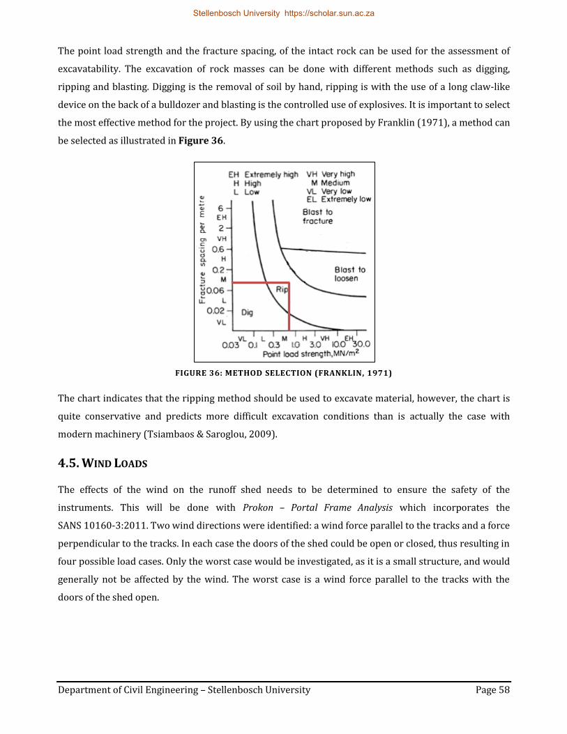
Department of Civil Engineering – Stellenbosch University Page 58
The point load strength and the fracture spacing, of the intact rock can be used for the assessment of
excavatability. The excavation of rock masses can be done with different methods such as digging,
ripping and blasting. Digging is the removal of soil by hand, ripping is with the use of a long claw-like
device on the back of a bulldozer and blasting is the controlled use of explosives. It is important to select
the most effective method for the project. By using the chart proposed by Franklin (1971), a method can
be selected as illustrated in Figure 36.
FIGURE 36: METHOD SELECTION (FRANKLIN, 1971)
The chart indicates that the ripping method should be used to excavate material, however, the chart is
quite conservative and predicts more difficult excavation conditions than is actually the case with
modern machinery (Tsiambaos & Saroglou, 2009).
4.5. WIND LOADS
The effects of the wind on the runoff shed needs to be determined to ensure the safety of the
instruments. This will be done with Prokon – Portal Frame Analysis which incorporates the
SANS 10160-3:2011. Two wind directions were identified: a wind force parallel to the tracks and a force
perpendicular to the tracks. In each case the doors of the shed could be open or closed, thus resulting in
four possible load cases. Only the worst case would be investigated, as it is a small structure, and would
generally not be affected by the wind. The worst case is a wind force parallel to the tracks with the
doors of the shed open.
Stellenbosch University https://scholar.sun.ac.za

Department of Civil Engineering – Stellenbosch University Page 59
TABLE 18: PARAMETERS USED IN PROKON CALCULATION
Peak wind speed 𝒗𝒑(𝒛) = 𝟒𝟎𝒎/𝒔
Terrain category B
Reference height 𝑧𝑒 = 5.454 𝑚
Peak wind speed pressure
𝑞𝑝 =1
2× 𝜌 × 𝑣𝑝
2(𝑧)
=1
2× 1.06 × 402
= 848 𝑘𝑔/𝑠2/𝑚
= 8318.88 𝑁/𝑠2/𝑚
Pitch of roof (Duel pitch roof) sin−1 (654
3114) = 12°
Parameters used to determine coefficients
External pressure coefficient
Internal pressure coefficient 𝐶𝑝𝑖 = 0.9 × 𝐶𝑝𝑒 (*NOTE 1)
External pressure 𝑤𝑖 = 𝑞𝑝 × 𝐶𝑝𝑒
Internal pressure 𝑤𝑒 = 𝑞𝑝 × 𝐶𝑝𝑖
NOTE 1: If the openings are located in zones with different values of external pressure, an area weighted average
value of 𝐶𝑝𝑒 shall be used.
With the use of the values in Table 18 and Prokon – Portal Frame Analysis, the wind pressure on the
shed was calculated for the worst case. Figure 37 illustrates these calculated pressures. The analysis
includes the self-weight of the structure as the section properties of the columns, rafters, purlins, side
rails and eaves beams have been specified. The maximum deflection obtained from the analysis was
2.2 mm. This indicates that the design of the runoff shed is sufficient to withstand wind forces at the
MSGO site.
Stellenbosch University https://scholar.sun.ac.za

Department of Civil Engineering – Stellenbosch University Page 60
FIGURE 37: WIND PRESSURE ON THE RUNOFF SHED
4.6. RISK MANAGEMENT
A risk is as an event or situation that can occur, which can either have a positive or negative impact on
the project, it can have more than one cause and more than one impact. Management of risks is a very
important aspect of the process, as it will determine the structural integrity and the life span of the
foundation. Risk management is an on-going process, which consists of identifying the risks, minimizing
them and monitoring those which cannot be excluded. It is important to consider a wide variety of
factors, including business and administrative aspects. Business aspects include procurement,
estimating and tendering, budget control and economic assessment; where administrative aspects
include organisation and financial management. Figure 38 shows how risks should be managed.
FIGURE 38: RISK MANAGEMENT
Risk Identification
Qualitative Risk Analysis
Quantitative Risk Analysis
Risk Response Planning
Risk Monitoring &
Control
Stellenbosch University https://scholar.sun.ac.za

Department of Civil Engineering – Stellenbosch University Page 61
Identified risks should be quantified. Table 19 shows a risk assessment matrix where the probability
and the consequences are taken into consideration. Each of the above mentioned factors gets a score
and the higher the total score, the more attention the risk needs. This table is used to score the
importance of the risks in the risk register as seen in Table 20. It is important to define an action to
mitigate each risk. Finding an economically viable solution to prevent the occurrence of risks is an
important aspect of risk management.
TABLE 19: RISK ASSESSMENT MATRIX
Likelihood
Consequences
Insignificant (1) (Minor problem
easily handled by normal day to day
processes)
Minor (2) (Some disruption
possible, e.g. damage equal to
R50 000)
Moderate (3) (Significant
time/resources required, e.g.
damage equal to R100 000)
Major (4) (Operations
severely damaged, e.g. damage equal
to R500 000)
Catastrophic (5) (Business survival is at risk, e.g. damage greater or equal to
R1 million)
Almost Certain (5) (e.g. >90%
chance)
High (6) High (7) Extreme (8) Extreme (9) Extreme (10)
Likely (4) (e.g. between 50% and 90%
chance)
Moderate (5) High (6) High (7) Extreme (8) Extreme (9)
Moderate (3) (e.g. between 10% and 50%
chance)
Low (4) Moderate (5) High (6) Extreme(7) Extreme (8)
Unlikely (2) (e.g. between 3% and 10%
chance)
Low (3) Low (4) Moderate (5) High (6) Extreme (7)
Rare (1) (e.g. <3% chance)
Low (2) Low (3) Moderate (4) High (5) High (6)
This risk register, in Table 20, only focuses on a few risks and there are many more risks that may
occur, thus the risks in this register should not be regarded as the only possible risks that may occur.
The importance of a competent, reliable and experienced geotechnical engineer is of utmost importance
(Wium, 2014), as engineering judgement plays a big role in the decisions made.
Stellenbosch University https://scholar.sun.ac.za

Department of Civil Engineering – Stellenbosch University Page 62
TABLE 20: RISK REGISTER
Risk Mitigating measures Importance according to
Table 18 (Likelihood + Consequence)
Incomplete geotechnical data:
Varying soil conditions: No information on rock
profile below 1,5m depth
Drilling of one geotechnical borehole on centre of base to
10 m depth.
(2+2) Low
Performance risks
Bearing capacity failure Found on competent rock. Negligible
Settlement Found on competent rock. Negligible
Settlements < 0,5 mm
Swell of shale Conduct free swell tests. (2+2) Low
Slope stability Selection of site on stable ground
with low relief. Negligible
Damage due to seismicity Follow code requirements. Negligible
Low PGA (Figure 4)
Construction risks
Increased volume of rock excavation
Make appropriate allowance in contract for rock excavation
volumes.
(3+2) Moderate
Soft material below designed founding level
Make allowance for excavation of soft material and replacement with mass concrete in contract
document.
(3+2) Moderate
Construction quality Registered geotechnical
engineer on site. (3+4)
Extreme
Availability of resources
Order and deliver materials before construction where
possible. Procure from reliable sources.
(2+3) Moderate
Equipment failure Procure from reliable sources, make allowance for delays in
project planning.
(2+3) Moderate
General risks
Site access difficulties
Complete construction/ rehabilitation of access road before construction of S/LLR
foundation commence.
Negligible
Productivity of labour, labour disputes or strikes
State expectations from labourers in contract before
work commences. Make allowance for delays in project
planning.
(4+2) High
Security of site Procure a reliable security
company to ensure safety during project.
(2+2) Low
Consequential losses The contract should define the indemnities for consequential
losses.
(1+4) High
Stellenbosch University https://scholar.sun.ac.za

Department of Civil Engineering – Stellenbosch University Page 63
CHAPTER 5: CONCLUSION AND RECOMMENDATIONS
From the results obtained in Chapter 4 the following conclusions and recommendations can be made.
5.1. BEARING CAPACITY
By using the UCS or point load index, the RQD and information about the joints, the rock can be rated by
the RMR system proposed by Bieniawski (1989). From this system a 𝑐 and ∅ value can be determined
and used in Terzhagi’s equation for bearing capacity, Equation 17. By using the bearing capacity
factors proposed by Stagg and Zienkiewicz (1968), a bearing capacity of 8.74 MPa was calculated for the
rock mass. The applied bearing pressure of 17 kPa is much smaller than the bearing capacity of the
rock and thus a safe assumption can be made that the rock mass is more than sufficient to withstand the
load of the structure.
5.2. SETTLEMENT
Settlement is more often of concern than the bearing capacity. The settlement can be calculated with
Equation 23, which is based on an elastic stress distribution. Steinbrenner’s (1934) method for
determining the vertical stress was used. The UCS results and chart proposed by Peck (1976) and Deere
(1968), were used to determine the Young’s modulus and with the use of Excel, the total settlement was
calculated as 0.1 mm. This is a conservative value as the weight of the soil removed was not subtracted
from the applied pressure.
From the result of this calculation it is clear that settlement would not be a factor influencing the
operation of the S/LLR. As the weight of the foundation itself is 84% of the applied pressure, little to no
settlement will occur after the concrete has hardened. It is thus recommended that the level of the
foundation should be calibrated after the hardening of the concrete and before the instrument is placed.
5.3. SLOPE STABILITY
The 3D model of the site showed a good representation of the actual terrain. The circular slip analysis,
on the southern side of the ridge, was completed with SLOPE/W, and a safety factor greater than 1.5
was obtained. This shows that the slope is stable and the probability for any circular failure is small.
The planar failure analysis, on the northern side of the ridge, was completed with Prokon and indicated
that the maximum cutting depth of the access road should be 1 m. The FOS for the cutting depth equal
to 2 m, is smaller than 1 and thus the slope is not stable. A solution to this problem could be the use of
Stellenbosch University https://scholar.sun.ac.za

Department of Civil Engineering – Stellenbosch University Page 64
anchor cables or a retaining wall, but it is an expensive option. Wedge failure along the road cutting is
not kinematically feasible and thus poses no threat to the stability of the slope.
It is recommended that an alternative route for access to the S/LLR should be investigated. However, if
it is chosen to be at the foot of the southern side of the hill, the toe can yield due to the reduced
stabilising moment caused by road excavation, which in turn will reduce the FOS for circular failure.
5.4. EXCAVATABILITY OF MATERIAL
Excavatability is the term used to describe the ease of excavating material. First the DCP values were
used to determine a DN value and give a corresponding strength of the soil layers. From this it can be
determined that the top 95 to 170 mm is a softer soil, which can be excavated by hand.
The point load strength and the fracture spacing of the intact rock mass, can be used for the assessment
of excavatability. This assessment was done with a chart proposed by Franklin et al., (1971). The chart
indicates that the ripping method should be used, thus a bulldozer would be needed. It is recommended
to excavate the top soil with the bulldozer as well, as it would save a lot of time and labour costs.
5.5. WIND LOADS To determine if the shed would withstand the forces of the wind at the MSGO site an analysis was done
with Prokon – Portal Frame Analysis which incorporates the SANS 10160-3:2011. The maximum
deflection obtained from the analysis was 2.2 mm. This indicates that the design of the runoff shed is
sufficient to withstand the forces induced by the wind.
5.6. FINAL REMARKS
The conclusion that can be drawn from this study is that the design of the foundations of the S/LLR at
MSGO will be the same as at HartRAO. This conclusion can be made as none of the factors that were
evaluated have shown a destabilising effect on the S/LLR. This option is beneficial to the project as no
consulting services would be required to design a new foundation, resulting in saving costs.
The shale at the MSGO site is impermeable to water, but water can still penetrate along bedding planes
causing the lumps to slake. It is recommended that when the excavation is made, a mass concrete layer
of at least 10 MPa should be keyed into the exposed founding rock mass. This will level the surface and
protect the exposed shale against slaking. Van Wyk (2013) determined that the shale at the MSGO site is
prone to slaking after five wet/dry cycles. It is thus important that the rock mass exposed after
excavation should immediately be covered to prevent slaking.
Stellenbosch University https://scholar.sun.ac.za

Department of Civil Engineering – Stellenbosch University Page 65
The petrographic studies have shown that clay minerals such as kaolinite and chlorite are present in the
samples. Since these are non-expansive minerals, it can be concluded that the rock mass is non-
expansive. As the effect of a swelling rock mass can have a destabilising effect on the foundation, it is
recommended that a free swell test should be done to determine quantitatively if this could be a
problem.
The depth of the influence sphere underneath a foundation is twice the width, being roughly 10 m in
this case. The final recommendation is to drill at least one core of 10 m deep at the centre of the
foundation. This will verify the strength of the founding material and that no discontinuities exist
underneath the foundation as there is no information on the rock profile deeper than 1.5 m.
Stellenbosch University https://scholar.sun.ac.za

Department of Civil Engineering – Stellenbosch University Page 66
BIBLIOGRAPHY
ALLEY, C.O., 1972. Story of the development of the Apollo 11 laser ranging retro-reflector experiment,
in Adventures in Experimental Physics, edited by B. Maglich, pp. 132-149, 1972.
American Society of Testing and Materials (ASTM)., 2002. Standard Test Method for Unconfined
Compressive Strength of Intact Rock Core Specimens, D2938-95(R02).
ANONYMOUS, 1993. History of Laser Ranging and MLRS. 1993. [Online]. Available:
http://www.csr.utexas.edu/mlrs/history.html [2014, June 6].
ANONYMOUS, 2010. Matjiesfontein info, [Online]. Available: http://www.matjiesfontien.com/ [ 2013,
October 12]
ANONYMOUS, 2013. How does BGS classify landslides? Online] Available:
http://www.bgs.ac.uk/science/landUseAndDevelopment/landslides/How_does_BGS_classify_l
andslides.html [September, 2013].
ANONYMOUS, 2014. Weatherbase, Sutherland, South Africa Travel Weather Averages. 2015. [ONLINE]
Available:
http://www.weatherbase.com/weather/weather.php3?s=687220&cityname=Sutherland-
South-Africa. [2014, October 18].
ANONYMOUS, 2015. Western Cape Tourist Map - Western Cape South Africa • mappery. 2015.
[ONLINE] Available at: http://www.mappery.com/Western-Cape-Tourist-Map. [Accessed 18
September 2015].
BIENIAWSKI, Z.T., 1989. Engineering Rock Mass Classifications. New York: Wiley.
BOTHA, R., 2015. Laser Pulse, E-mail to R. Botha [Online], 8 September. Available E-mail:
BRINK, A.B.A., 1981. Engineering Geology of South Africa. Volume 2. Pretoria: Building Publications.
BRINK, A.B.A., 1983. Engineering Geology of South Africa. Volume 3. Pretoria: Building Publications.
CHAPRONT, J., FRANCOU, G., 1973. Lunar Laser Ranging stations and reflectors [Online]. Available:
http://www.checktheevidence.com/pdf/Laser%20ranging%20-
%20Apollo%20Reflectors%20etc%20on%20The%20Moon.pdf [2014, March 16]
Stellenbosch University https://scholar.sun.ac.za

Department of Civil Engineering – Stellenbosch University Page 67
CHEN, K. AND LIU, J. 2010., PC Guided Design Method in Analysis for Rock Slope Stability in
Geotechnical Engineering. Paper presented at 2010 2nd International Conference on
Mechanical and Electronics Engineering, ICMEE 2010, August 1, 2010 - August 3. 2010.
COMBRINCK, L., FOURIE, C.J.S., CROUKAMP, L. and SAUNDERS, I., 2007. Report on preliminary
geotechnical and tropospheric site investigation for a proposed space geodetic observatory
near Matjiesfontein in the Great Karoo. South African Journal of Geology, 110(2), pp. 225-234.
COMBRINCK, L., 2015. Personal interview. 6 May. Hartebeesthoek Radio Astronomy Observatory.
Core Logging Committee of the South African Section of the Association of Engineering Geologists.,
1976. A guide to core logging for rock engineering, in Symposium for Rock Engineering.
Johannesburg: 71-86.
CRAIG, R.F., 2004. Craig's soil mechanics. 7 edn. New York: Taylor & Francis.
CROUKAMP, L., 2013. Personal interview. 7 August, Matjiesfontein.
CROUKAMP, L., ROSSOUW, J.J., FOURIE, C.J.S., COMBRINCK, L., 2011. Foundation requirements for a
lunar laser ranger facility at matjiesfontein, South Africa. South African Journal of Geology, 114
(3-4): 573–576.
DAY, P.W., 1987. Prediction of Settlement. Lecture Course Programme 1987 Geotechnical Division.
DAY, P.W., 2014. Foundation Types. Unpublished class notes (Foundation Design 811). Stellenbosch:
University of Stellenbosch.
DAS, B.M., 2002. Principles of Geotechnical Engineering. Bill Stenquist
DEERE, D.U., 1968, Geological Considerations, K.G. Stagg and O.C. Zienkiewicz, Rock Mechanics in
Engineering Practice, Wiley, New York.
DE WET, M., 2013. Personal interview. 1 October, Stellenbosch.
DICKEY, J.O., BENDER, P.L., FALLER, J.E., 1994. "Lunar Laser Ranging: A Continuing Legacy of the Apollo
Program", Science, Jul 22, pp.482-490.
DUNCAN, C., 1980. Toppling Rock Slope Failures Examples of Analysis and Stabilization. Unpublished
paper delivered at The 21st U.S. Symposium on Rock Mechanics May 27 - 30, 1980, Rolla.
ECOSENSE, 2010. Proposed Matjiesfontein geodesy station. Environmental screening report edn.
Stellenbosch: Ecosense Consulting Environmentalists.
Stellenbosch University https://scholar.sun.ac.za

Department of Civil Engineering – Stellenbosch University Page 68
ECOSENSE, 2015. Proposed Matjiesfontein geodesy station. Environmental screening report edn.
Stellenbosch: Ecosense Consulting Environmentalists.
FRANKLIN, JA., BROCH, E., WALTON, G., 1971 Logging the mechanical character of rock. Trans Inst Min
Metall 80:A1–A9
HOEK, E. and BRAY, J.W., 1981, Rock Slope Engineering: The Institute of Mining and Metallurgy, London,
England.
HUNT, R.E., 2005, Geotechnical Engineering Investigation Handbook 2nd edn. CRC Press
JOHNSON, M.R., Anhaeusser, C.R., Thomas, R.J., 2006. The Geology of South Africa: Geological Society of
South Africa, Johannesburg and the Council for Geoscience, Pretoria.
JONES, E.M., GLOVER, K., 2013. [Online]. Available: http://www.hq.nasa.gov/alsj/ [2015, March 30].
KIJKO, A., GRAHAM, G., BEJAICHUND, M., ROBLIN, D.L., BRANDT, M.B.C., 2003. Probabilistic Peak
Ground Acceleration and Spectral Seismic Hazard Maps for South Africa.
LORY, J., [S.a.]. Structures of clays [Online] Available: http://soils.missouri.edu/about.asp
[2015, Augustus 2].
MATHEWSON, C.C., 1981. Engineering geology. Merrill
MURPHY, T.W., 2013. Lunar laser ranging: the millimeter challenge. Reports on progress in physics.
Physical Society (Great Britain), 76(7), p.076901. Available at:
http://www.ncbi.nlm.nih.gov/pubmed/23764926.NASA. 1971. [Online]. Available:
http://spaceflight.nasa.gov/gallery/images/apollo/apollo14/html/as14-67-09386.html
[2015, Augustus 21].
NORMAN, N. & WHITFIELD, G., 2006. Geological Journeys. 1st ed. Cape Town: Struik Nature.
PECK, R.B., 1976, Rock Foundations for Structures, Rock Engineering for Foundations and Slopes. Proc.
ASCE, Vol. 2: 1-21.
PETTERSEN, C., 2014. Study on the Swelling Potential of some Selected Rocks Catrine Pettersen.,
Norwegian University of Science and Technology
SHORT, N.M., 2005. Remote Sensing Tutorial [Online] Available:
http://fas.org/irp/imint/docs/rst/Intro/Part2_1c.html [2014, July 15]
Stellenbosch University https://scholar.sun.ac.za

Department of Civil Engineering – Stellenbosch University Page 69
SILVERBERG, E.C., 1974, Operation and performance of a lunar laser ranging station, Appl. Opt., 13, 565-
574, 1974.
STAGG, K.G., ZIENKIEWICZ, O.C., 1968, Rock Mechanics in Engineering Practice, John Wiley & Sons, New
York.
STEINBRENNER, W., 1934. Tafeln zur setzungsberschnung. Die Strasse, 1: 121-124.
TARBUCK, E.J., LUTGENS, F.K., TASA, D., 1996. Earth. Prentice Hall
TERZAGHI, K., 1943, Theoretical Soil Mechanics, John Wiley & sons, New York, 5100pp.
TSIAMBAOS, G., SAROGLOU, H., 2009. Excavatability assessment of rock masses using the Geological
Strength Index (GSI), in Bulletin of Engineering Geology and the Environment (2010) 69:13–
27
ULUSAY, R., HUDSON, J.A., 2006, The Complete ISRM Suggested Methods for Rock Characterization,
Testing and Monitoring: 1974-2006. Turkey: pp 53-60
VAN WYK, P., 2013. Rock Mechanics for Construction of the Gravimeter Vault at the Matjiesfontein
Space Geodesy and Earth Observation Observatory. Unpublished Master’s Thesis.
Stellenbosch: University of Stellenbosch.
VEILLET, C., MANGIN, J.F., CHABAUBIE, J.E., DUMOLIN, C., FERAUDY, D. AND TORRE, J.M., 1993, Lunar
Laser Ranging at CERGA for the Ruby Period (1981-1986), in Contributions of Space Geodesy
to Geodynamics: Technology (eds D. E. Smith and D. L. Turcotte), American Geophysical Union,
Washington, D. C.. doi: 10.1029/GD025p0189
VISSER, D., 2012. GPS survey and slope analysis at the Matjiesfontein Space Geodesy site for the
emplacement of a Lunar Laser Ranger Unpublished BEng mini thesis. Stellenbosch:
Stellenbosch University.
VISSER, J.N., VAN NIEKERK, B.N. & VAN DER MERWE, S.W., 2004. Sediment transport of the late
Palaeozoic glacial Dwyka Group in the southwestern Karoo Basin. South African Journal of
Geology, 100(3), pp. 223-236.
WATERS, J., 2011. Geotechnical Investigation of Palaeo-landslides at the Matjiesfontein Geodesy
Observatory. Unpublished BEng mini thesis. Stellenbosch: Stellenbosch University.
WIUM, J., 2014. Personal interview. 31 July 2014, Stellenbosch.
Stellenbosch University https://scholar.sun.ac.za

Department of Civil Engineering – Stellenbosch University Page 70
ZHANG, C.L., WIECZOREK, K. AND XIE, M.L., 2010. Swelling experiments on mudstones., Journal of Rock
Mechanics and Geotechnical Engineering, 2 (1): 44–51.
Stellenbosch University https://scholar.sun.ac.za

Department of Civil Engineering – Stellenbosch University Page 71
APPENDIX A: AS-BUILT DRAWINGS
Stellenbosch University https://scholar.sun.ac.za

3297
CLE
AR
AN
CE
HE
IGH
T 4
800
654
5454
3075
540 997 1388 150 150 1837 998 540
3075
5000
± 25 mmNON-SHRINKABLE
GROUT
2x180 IPE - HORIZONTAL RAIL
100x50x20x2,0mm CFLC
150
2051
1497
IPE 180 BEAMIP
E 1
80 C
OLU
MN
IPE
180
CO
LUM
N
IPE
180
CO
LUM
N
45701075 1075
1419
1419
509
153 153
1419
1419
554
3144 3144
150
20035
0
SECTION A-ASCALE 1:20
60x60x6,0mm L HRAVERTICAL BRACING
6260
1020
150mm R/C SLAB WITH MESHREF 245 NOT LESS THAN
35mm FROM TOP OF SLAB
IPE 180
RIDGE CAP - FLASHING
DETAIL A
DETAIL B
DETAIL C
DETAIL D
100x50x20x2,0mmCFLC SIDE RAILS
KLIP-LOK 700 LIGHTINDUSTRIAL ROOF SHEETING
375 140 345 345 1401985 600 1985 215
150mm R/C SLAB WITH MESHREF 245 NOT LESS THAN35mm FROM TOP OF SLAB
2985 2985
60x150x6mm RECTANGULARSTEEL PLATE WELDED TO IPE180
@ MAXIMUM 1,0m c/c ANDBOLTED TO 100x50x20x2.0mm
CFLC WITH 2/M12 BOLTS
R600
8Y12 @ 325c/c (4Y12-T2, 4Y12-B2) 8Y12 @ 325c/c (4Y12-T2, 4Y12-B2)
F.G.L.150mm MIN TOPSOILSTRIPPED. REFERCONCRETE NOTES
400
400
357
50
18040
50
12° 12°
2x 100x50x20x2,0mmCFLC SIDE RAILSBACK TO BACK
81
10001000 7575
1000x1000x1200mmDEEP REINFORCED
CONCRETE BASE
1200x1200x1200mm DEEPEXCAVATION UNDER STRIPFOOTING, FINAL DEPTH TOBE DETERMINED ON SITEBY THE ENGINEER ANDBACKFILLED WITH A G6/G5IMPORTED MATERIAL ORSIMILAR APPROVED.
215
445 445
400x600mm DEEPREINFORCED
CONCRETE BEAM
923
250
600
1200
600
150
115175 75275
1559 562 1559
3680
18401840
75mm Ø CHS AT FLOOR LEVEL
300 300300 50mm SCREED ASSHOWN TO FALLS
5040
4
2056
1846
IPE 180 BEAM
3983
5970
180 IPE - HORIZONTAL RAIL
100x50x20x2,0mmCFLC SIDE RAILS
± 25 mmNON-SHRINKABLE GROUT
AB
C
1540
3297
4661
16956
106995926
803
100x50x20x2,0mm CFLC PURLIN
100x50x20x2,0mm CFLC SIDE RAIL60x60x6,0mm L RAFTERAND VERTICAL BRACING
16772 7052
23824
15°
180 IPE COLUMN
2x180 IPE RAIL
180 IPE COLUMN
SECTION B-BSCALE 1:50
4985500 441
150
745 413 445 17894
500
F.G.L.
1460
1458
1435
419
4654
24128
1000
BACKSTOP - 100x200x240x312x 10,0mmTHICK STEEL PLATE WELDED TO
250x100x10mm STEEL PLATE & BOLTEDWITH 6/M16 CHEMICAL ANCHOR BOLTS
GRADE 8.8 TO R/C FOOTING
675
2056
1846
350
2963 2963
143245
F.G.L.150mm MINIMUM TOPSOILSTRIPPED. REFER TOCONCRETE NOTES - NOTE 3
VENT
1000
81
83225007929100045381000
1000x1000x1200mmDEEP R/C/ BASE
600
600
600
1540
3680
923
600
1 3
D D
750
2360
500
2360
750
495 2218 2320 750 17644
24177
625
375
BASE & STRIPFOOTING LAYOUTSCALE 1:50A
A
4570
4538
C
C5000
5970
5000
1075
400x600mm DEEP REINFORCED CONCRETE BEAM
750x350mm THICK R/C STRIPFOOTING
500x350mm THICK R/C STRIPFOOTING
750x350mm THICK R/C STRIPFOOTING
DETAIL E
BACKSTOP - 100x200x240x312x 10,0mmTHICK STEEL PLATE WELDED TO
250x100x10mm STEEL PLATE & BOLTEDWITH 6/M16 CHEMICAL ANCHOR BOLTS
GRADE 8.8 TO R/C FOOTING
325
750
4783 750 8322 500 8322 500
500x
1000
mm
DE
EP
R/C
ST
RIP
FO
OT
ING
4570
750
5
500495
107
2963 2963
NOTE:REFER TO CONCRETE NOTES
BACKSTOP - 100x200x240x312x 10,0mmTHICK STEEL PLATE WELDED TO
250x100x10mm STEEL PLATE & BOLTEDWITH 6/M16 CHEMICAL ANCHOR BOLTS
GRADE 8.8 TO R/C FOOTING
750
750
750x500x1000mmDEEP FOOTING
500x
1000
mm
DE
EP
R/C
ST
RIP
FO
OT
ING
500x
1000
mm
DE
EP
R/C
ST
RIP
FO
OT
ING
500x
1000
mm
DE
EP
R/C
ST
RIP
FO
OT
ING
143500 500500 500
245
4720
625
375
700
3680
700
1000
75
1000 245 3941 143 1000
1000x1000x1200mmDEEP R/C BASE
485 441
1000x1000x1200mmDEEP R/C BASE
1000x1000x1200mmDEEP R/C BASE
1000x1000x1200mmDEEP R/C BASE
2808 2808
2792
2792 60
825999
400
287440
0
B B
89°
91°
271
445
445
413 3064
350mm R/C SLAB
350mm R/C SLAB
445
303
3680
260
202
BEAM
BEAM
BEAM
BEAM
BEAM
BEAM
327269
295 321
AB
C
1
2
3
B
269 327
307
1978
1978
307
500
500
SURFACE BED LAYOUTSCALE 1:50
A
A
200
C
C
3921
5970
5000 B
200
745
3957
NOTE:REFER TO CONCRETE NOTES
445 643 107
445
215
485
441
6431971 1971
150mm R/C SLABWITH MESH REF 245
NOT LESS THAN 35mmFROM TOP OF SLAB
150mm R/C SLABWITH MESH REF 245NOT LESS THAN 35mmFROM TOP OF SLAB
3680
445
700
375
36804137455
451
2500 2500
75mm Ø CHS ATFLOOR LEVEL
75mm Ø CHS ATFLOOR LEVEL
4550
4518
170mm HIGHBRICK WALL
± 25 mmNON-SHRINKABLE GROUT
DETAIL DSCALE 1:10
180 IPE - COLUMN
150mm CASTER WHEEL
1075
8Y12 @ 325c/c (4Y12-T2, 4Y12-B2)
10
F.G.L.150mm MIN TOPSOILSTRIPPED. REFER NOTE 3
IJ
350
R10 STIRRUPS@ 350 c/c
180 IPE - HORIZONTAL RAIL
6/ M16 BOLTS GRADE 8.8
REFER TO DETAIL K
T-SECTION CUT FROM 180IPE REFER TO DETAIL
180
96
23252523
5040
4050
96x186x8mmRECTANGULARSTEEL PLATE
IPE 180 BEAM
6/ M16 BOLTSGRADE 8.8
DETAIL KSCALE 1:5
BASE PLATE IPE180 COLUMN
60x60x6,0mm L HRA
SECTION D-DSCALE 1:50
350
1000
1200
600
400x600mm DEEPREINFORCEDCONCRETE BEAM
2x180 IPE RAIL
750x350mm DEEP R/C FOOTING
F.G.L.150mm MIN TOPSOILSTRIPPED. REFER NOTE 3
1200x1200x1200mm DEEP EXCAVATION UNDERSTRIP FOOTING, FINAL DEPTH TO BE DETERMINEDON SITE BY THE ENGINEER AND BACKFILLED WITH AG6/G5 IMPORTED MATERIAL OR SIMILAR APPROVED.
1000x1000x1200mm DEEP R/C BASE
DETAIL M
600 85
0
50mm SCREED TO FALL
1000
1200x1200x1200mm DEEP EXCAVATIONUNDER STRIP FOOTING, FINAL DEPTH TOBE DETERMINED ON SITE BY THE ENGINEERAND BACKFILLED WITH A G6/G5 IMPORTEDMATERIAL OR SIMILAR APPROVED.
400x600mm DEEPREINFORCED
CONCRETE BEAM
1000x1000x1200mm DEEP R/C BASE
R10 STIRRUPS@ 350 c/c
8Y12 @ 325c/c (4Y12-T2, 4Y12-B2)
F.G.L.150mm MIN TOPSOILSTRIPPED. REFER NOTE 3
DETAIL M: BASE & BEAMSCALE 1:10
Y25Y25Y25Y25
Y16 Y16
850
350
Y10 Y10Y10Y10Y10
Y10 Y10Y10Y10Y10
Y10 Y10Y10Y10Y10
Y10 Y10Y10Y10Y10
600
1200
493
409
100x50x20x2,0mmCFLC SIDE RAIL
211x493x410mm HAUNCH CUT FROM180 IPE, WELDED TO 215x96x8mmSTEEL PLATE & BOLTED WITH 6 M16GRADE 8.8 BOLTS TO IPE 180 COLUMN
211
5011
150
DETAIL BSCALE 1:10
100x50x20x2,0mm CFLC
50
60x150x6mm RECTANGULARSTEEL PLATE WELDED TOIPE180 @ MAX 1,0m c/c ANDBOLTED TO 100x50x20x2.0mmCFLC WITH 2/M12 BOLTS12°
R600
410
150
40 35
SECTION TYPICAL SAW JOINTSCALE 1:5
TITEL
KLIENT TEK. NO.
KONSULTANT TEK. NR.
SKAAL VERWYS.
1.0 3.0
2.0 4.0
KLIENT
PROJEK
Tel: +27 (15) 291-3363Fax: +27 (15) 291-3403
E-mail : [email protected]
CONSULTANT DWG. NO.
2.0
OCTOBER 2010
AS SHOWN
CLIENT DWG. NO.
4.0
3.0
DATE/DATUM
SCALE/SKAAL
SCALE REF.
TITLE
meter1.0
0
PROJECT
CLIENT
BASES, STRIPFOOTING,STEEL STRUCTURE,
DETAILS & SECTIONS -AS BUILT PLAN
OBSERVATORYTELESCOPE HOUSING
P2325/S1
SPACE GEODESYHartRAO
P.O. BOX 477FAUNA PARK0787
CHECKED/NAGESIEN
DRAWN/GETEKEN
DESIGNED/ONTWERP
CAD FILE NAME/CAD LÊER NAAM
APPROVED/GOEDGEKEUR
P DU PREEZ
DIENS
STRUCTURE
AMENDMENTS/WYSIGING
SERVICE
Her.Rev.
BeskrywingDescription
DatumDate
DeurBy
DJ ERASMUS
DRA WINGS M US T NOT BE S CALE D. F IG UREDDIMENSIONS ONLY MAY BE USED. DIMENSIONSS H O U L D B E V E R I F I E D I N F I E L D A N D A N YDISCREPANCIES REPORTED TO THE ENGINEERIMMEDIATLY. THIS DRAWING IS COPYRIGHT AND THEP RO P E RT Y OF E N DE CO N A ND M US T NO T B ERETAINED, COPIED OR USED WITHOUT AUTHORITY.
DJ ERASMUS
07
01 GENERAL UPDATE 27/01/2011 PDP
CONCRETE NOTES:
1. ALL CONCRETE WORK TO BE DONE IN ACCORDANCEWITH S.A.B.S. 1200, 28 DAY STRENGTH :-
1.1. REINFORCED CONCRETE = 25Mpa/19mm.1.2. REINFORCED CONCRETE GROUND FLOOR =
30Mpa/19mm.1.3. CONCRETE SURFACE BED = 20Mpa/19mm.1.4. BLINDING/STRIP FOOTINGS = 20Mpa/19mm.1.5. REINFORCED CONCRETE COLUMNS = 30Mpa/19mm.
2. MIN. CONCRETE COVER TO MAIN REINFORCEMENT:-2.1. BASES = 50mm TOP & 75mm BOTTOM.
3. NO CONCRETE MAY BE POURED BEFORE THE ENGINEERHAS APPROVED FOUNDATION CONDITIONS AND ALLREINFORCEMENT.
4. NO DIMENSIONS MUST BE SCALED ON THE DRAWING,CONTACT THE ENGINEER. ALL DIMENSIONS AND LEVELSTO BE CHECKED ON SITE BEFORE STARTING WORK.
5. CONCRETE WORK SHOULD BE TO DEGREE OFACCURACY 2 AS PER SABS 1200 G CLAUSE 6.
STEEL NOTES:1) ALL WELDS TO BE FULL STRENGTH FILLET WELDS ALLROUND WITH THICKNESS OF SMALLER CONNECTEDELEMENT2) ALL STEEL TO BE GRADE 350W3) ALL BOLTS TO BE GRADE 8.84) PAINT SPECIFICATION -
I. CORROSION PROTECTION TO SABS 1200 HC AND MUSTBE READ IN CONJUNCTION WITH SABS 0120 SECTION HCPART 3
II. PAINT SYSTEM ALKYD-013-016 IS USED 1st COAT: ZINCPHOSPHATE 30 MICRON (DFT) TO SABS 678 2nd COAT:GENERAL TYPE UNDERCOAT 30 MICRON (DFT) TO SABS 681. 3rd COAT: ALKYD ENAMEL 30 MICRON TOSABS 630, COLOUR ACC. TO ARCHITECT.5) CLEANING OF STEEL TO SABS 064 AND SIS 05 59 00 ST2.
NOTE:REFER TO STEEL NOTES
02 03/02/2011 PDPADDED 180 IPE'S FRONT & BACK,CHANGED DOORS
NOTE: PROVIDE CONSTRUCTION JOINTS
WHERE CASTING OF CONCRETE ISINTERUPTED AND CONTINUED AT ALATER STAGE.
SAWCUT JOINTS TO BE CUT WITHIN 24HOURS OF CASTING.
LEGEND:SJ - SAW CUT JOINTIJ - ISOLATION JOINTMJ - MOVEMENT JOINTCJ - CONSTRUCTION JOINT
NOTE:REFER TO DRAWING L2325/S2 FORMORE DETAILS AND SECTIONS
03 ADDED DETAILS, CFLC, ETC 04/02/2011 PDP
04 ADJUSTED STRIPFOOTINGS (1mx1mx1m) 30/03/2011 PDP
05 BEAMS ADDED, SURFACE BED CHANGED 6/04/2011 PDP
06 ADDED DIMENSION, UPDATED SECT B-B 20/05/2011 PDP
07 UPDATED AS BUILT CHANGES 01/08/2011 PDP
Stellenbosch University https://scholar.sun.ac.za
Stellenbosch University https://scholar.sun.ac.za

4800
654
100x50x20x2,0mm CFLC PURLIN
100x50x20x2,0mm CFLC SIDE RAIL60x60x6,0mm L RAFTERAND VERTICAL BRACING
15°
180 IPE COLUMN
2x180 IPE RAIL
60x60x6,0mm L HRA
T-SECTION CUT FROM 180IPE REFER TO DETAIL D
BACKSTOP - 100x200x240x312x 10,0mmTHICK STEEL PLATE WELDED TO
250x100x10mm STEEL PLATE & BOLTEDWITH 6/M16 CHEMICAL ANCHOR BOLTS
GRADE 8.8 TO R/C FOOTING
5539
3500
26122951
5563
4200
10795
180 IPE BEAMHAUNCH
180 IPE BEAM
5882
2941 2941
F.G.L.
170m
m
BR
ICK
WA
LL
3297
15°
F.G.L.
BACKSTOP - 100x200x240x312x 10,0mmTHICK STEEL PLATE WELDED TO
250x100x10mm STEEL PLATE & BOLTEDWITH 6/M16 CHEMICAL ANCHOR BOLTS
GRADE 8.8 TO R/C FOOTING
F.G.L.150mm MINIMUM TOPSOILSTRIPPED. REFER TOCONCRETE NOTES - NOTE 3
923
PLAN SHOWING VISUAL CLEARANCESCALE 1:50
5250
3250
750
2360
500
2360
750
PROPOSED SITE LAYOUTSCALE 1:50
NOTE:REFER TO CONCRETE NOTES
1500
2200
EXISTING SATELLITESTATION TRAILER
EXISTING STORAGEAND OFFICE TRAILER
NEW LASER TELESCOPE CONTAINER - CONTROL ROOM
NEW TELESCOPE HOUSING
2260
4260
1000
1000
400 12000 400
12800
PLATFORM
PLATFORM
PLATFORM
ROOF TOP 4200mm HIGH
ROOF TOP 3200mm HIGH
24133
23422
626317561
6720
6450
EXISTING SECONDARY FENCE(TO BE REMOVED)
EXISTING MAIN SECURITY FENCE
EXISTINGSWIMMING POOLFENCE
EXISTINGSWIMMING POOLFENCE
N
1900
1000
7000
530
7250
1900
40
7520
35-5
0
150
65
40
SECTION G-G:TYPICAL ISOLATION JOINTSCALE 1:5
REINF CONCRETE BASE/SLAB
100 100
6mm SAW JOINT
20 10
10mm ISOLATIONJOINT
G
G
PLAN DETAIL SHOWING INTERSECTIONOF SAW- AND ISOLATION JOINTSCALE 1:5
150mm SLAB WITH MESHREF 245 NOT LESS THAN35mm FROM TOP OF SLAB
SECTION K-KSCALE 1:5
184
50 34 34 5016
96
2325
2523
96x184x8mmRECTANGULARSTEEL PLATE
IPE 180 BEAM
4/M16 BOLTSGRADE 8.8
186
96
23252523
5043
4350
96x186x8mmRECTANGULARSTEEL PLATE
IPE 180 BEAM
6/ M16 BOLTSGRADE 8.8
SECTION E-ESCALE 1:5
60x150x6mm RECTANGULARSTEEL PLATE WELDED TOIPE180 @ MAX 1,0m c/c ANDBOLTED TO 100x50x20x2.0mmCFLC WITH 2/M12 BOLTS
151
25 50
SECTION F-FSCALE 1:5
100x250x8mm THICKRECTANGULAR
STEEL PLATE
6/ M16 CHEMICALANCHOR BOLTS
GRADE 8.8
100x200x240x312x10.0mmTHICK STEEL PLATE
100
250
2525 2525
5043
4350
88
DETAIL ASCALE 1:5
K K
EE
84 84
96x184x8mm RECTANGULARSTEEL PLATE WELDED TO IPE 180COLUMN AND BOLTED TOGETHERWITH 4/M16 BOLTS GRADE 8.8
100x50x20x2,0mmCFLC
2/96x186x8mm RECTANGULARSTEEL PLATES WELDED TO A IPE180 BEAM AND BOLTED TOGETHERWITH 6 M16 GRADE 8.8 BOLTS
12°
200
50 50 50 50
10
100
2525
2525 F
F
DETAIL ESCALE 1:5
100x250x8mm THICKRECTANGULAR
STEEL PLATE
6/ M16 CHEMICALANCHOR BOLTS
GRADE 8.8
100x200x240x312x10.0mmTHICK STEEL PLATE
B
A
A
ROOF LAYOUTSCALE 1:50
100x50x20x2,0mmCFLC SIDE RAIL
60x60x6,0mm LVERTICAL BRACINGBACK TO BACKWHERE CROSSING
60x60x6,0mmVERTICAL BRACING
180 IPE COLUMN
100x50x20x2,0mm CFLC PURLIN
100x50x20x2,0mm CFLC PURLIN
100x50x20x2,0mm CFLC PURLIN
100x50x20x2,0mm CFLC PURLIN
100x50x20x2,0mm CFLC PURLIN
100x50x20x2,0mm CFLC PURLIN
60x60x6,0mmL ROOF BRACING
B
C
C
5000485 441
5926
485
2500
2500
485
9090
KLIP-LOK 700LIGHT INDUSTRIALROOF SHEETING
2963 2963
2985
2985
540
998
1387
300
1388
997
540
6260
180 IPE BEAM
AB
C
1 32
100x50x20x2,0mm CFLC SIDE RAIL
180 IPE COLUMN
180 IPE - VERTICAL STRUT180 IPE -HORIZONTAL BEAM
849 8
868
200x849x868mm HAUNCH CUT FROM180 IPE, WELDED TO 200x96x8mmSTEEL PLATE & BOLTED WITH 6 M16GRADE 8.8 BOLTS TO IPE 180 COLUMN
100x50x20x2,0mm CFLC
189
4510
089
100
45
378
40 100 40
DETAIL CSCALE 1:10
C
CLE
AR
AN
CE
HE
IGH
T 4
800
654
5454
150
2136
2136
200
180 IPE - VERTICAL STRUT
ELEVATION C-CSCALE 1:50
INDUSTRIAL HINGESTO OPEN 270°
180 IPE - HORIZONTAL BEAM
90x90x8,0mm T-SECTION CUT FROM IPE 180 - DOOR FRAME
3230
1457
1768
1344
KLIP-LOK 700 LIGHTINDUSTRIAL ROOF SHEETING
FOR ROOF AND CLADDING
85
2985 2985
3075 3075
F.G.L.150mm MIN TOPSOILSTRIPPED. REFER NOTE 3
12° 12°
90x90x8,0mmT-SECTION CUT FROMIPE180 FOR DOORFRAME
75x50x20x2,0mmCFLC SIDE RAIL - DOOR
40x40x5,0mm LC VERTICAL BRACINGBACK TO BACK WHERE CROSSING
A
BSCREED TO FALLSCALE 1:20
SCREED TO FALL
50
SCREED TO FALL
600
TITEL
KLIENT TEK. NO.
KONSULTANT TEK. NR.
SKAAL VERWYS.
1.0 3.0
2.0 4.0
KLIENT
PROJEK
Tel: +27 (15) 291-3363Fax: +27 (15) 291-3403
E-mail : [email protected]
CONSULTANT DWG. NO.
2.0
FEBRUARY 2011
AS SHOWN
CLIENT DWG. NO.
4.0
3.0
DATE/DATUM
SCALE/SKAAL
SCALE REF.
TITLE
meter1.0
0
PROJECT
CLIENT
PROPOSED SITELAYOUT & ROOFAS-BUILT PLAN
OBSERVATORYTELESCOPE HOUSING
P2325/S2
SPACE GEODESYHartRAO
P.O. BOX 477FAUNA PARK0787
CHECKED/NAGESIEN
DRAWN/GETEKEN
DESIGNED/ONTWERP
CAD FILE NAME/CAD LÊER NAAM
APPROVED/GOEDGEKEUR
P DU PREEZ
DIENS
STRUCTURE
AMENDMENTS/WYSIGING
SERVICE
Her.Rev.
BeskrywingDescription
DatumDate
DeurBy
DJ ERASMUS
DRA WINGS M US T NOT BE S CALE D. F IG UREDDIMENSIONS ONLY MAY BE USED. DIMENSIONSS H O U L D B E V E R I F I E D I N F I E L D A N D A N YDISCREPANCIES REPORTED TO THE ENGINEERIMMEDIATLY. THIS DRAWING IS COPYRIGHT AND THEP RO P E RT Y OF E N DE CO N A ND M US T NO T B ERETAINED, COPIED OR USED WITHOUT AUTHORITY.
DJ ERASMUS
03
01 04/02/2011 PDP
CONCRETE NOTES:
1. ALL CONCRETE WORK TO BE DONE IN ACCORDANCEWITH S.A.B.S. 1200, 28 DAY STRENGTH :-
1.1. REINFORCED CONCRETE = 25Mpa/19mm.1.2. REINFORCED CONCRETE GROUND FLOOR =
30Mpa/19mm.1.3. CONCRETE SURFACE BED = 20Mpa/19mm.1.4. BLINDING/STRIP FOOTINGS = 20Mpa/19mm.1.5. REINFORCED CONCRETE COLUMNS = 30Mpa/19mm.
2. MIN. CONCRETE COVER TO MAIN REINFORCEMENT:-2.1. BASES = 50mm TOP & 75mm BOTTOM.
3. NO CONCRETE MAY BE POURED BEFORE THE ENGINEERHAS APPROVED FOUNDATION CONDITIONS AND ALLREINFORCEMENT.
4. NO DIMENSIONS MUST BE SCALED ON THE DRAWING,CONTACT THE ENGINEER. ALL DIMENSIONS AND LEVELSTO BE CHECKED ON SITE BEFORE STARTING WORK.
5. CONCRETE WORK SHOULD BE TO DEGREE OFACCURACY 2 AS PER SABS 1200 G CLAUSE 6.
STEEL NOTES:1) ALL WELDS TO BE FULL STRENGTH FILLET WELDS ALLROUND WITH THICKNESS OF SMALLER CONNECTEDELEMENT2) ALL STEEL TO BE GRADE 350W3) ALL BOLTS TO BE GRADE 8.84) PAINT SPECIFICATION -
I. CORROSION PROTECTION TO SABS 1200 HC AND MUSTBE READ IN CONJUNCTION WITH SABS 0120 SECTION HCPART 3
II. PAINT SYSTEM ALKYD-013-016 IS USED 1st COAT: ZINCPHOSPHATE 30 MICRON (DFT) TO SABS 678 2nd COAT:GENERAL TYPE UNDERCOAT 30 MICRON (DFT) TO SABS 681. 3rd COAT: ALKYD ENAMEL 30 MICRON TOSABS 630, COLOUR ACC. TO ARCHITECT.5) CLEANING OF STEEL TO SABS 064 AND SIS 05 59 00 ST2.
NOTE:REFER TO DWG L2325/S1 FOR MORE DETAILS AND SECTIONS
ADDED DETAIL H & MOVED DETAILSFROM L2325/S1 TO -/S2
02 15/02/2011 PDPCHANGED BUILDING POSITIONS03 06/04/2011 PDPUPDATED SHEET, DETAILS FROM S1
Stellenbosch University https://scholar.sun.ac.za
Stellenbosch University https://scholar.sun.ac.za

Department of Civil Engineering – Stellenbosch University Page 74
APPENDIX B: CONSTRUCTION SITE PHOTOS
FIGURE 39: CONSTRUCTION OF THE S/LLR FOUNDATION AT HARTRAO: TRACKS
FIGURE 40: CONSTRUCTION OF THE S/LLR FOUNDATION AT HARTRAO: BASE
Stellenbosch University https://scholar.sun.ac.za

Department of Civil Engineering – Stellenbosch University Page 75
FIGURE 41: CONSTRUCTION OF THE S/LLR FOUNDATION AT HARTRAO: COMPLETED
FIGURE 42: PLACING OF THE S/LLR ON THE BASE OF THE FOUNDATION
Stellenbosch University https://scholar.sun.ac.za

Department of Civil Engineering – Stellenbosch University Page 76
FIGURE 43: THE S/LLR AT HARTRAO, WITH RUN-OFF SHED IN BACKGROUND
Stellenbosch University https://scholar.sun.ac.za

Department of Civil Engineering – Stellenbosch University Page 77
APPENDIX C: UCS TEST SAMPLES
FIGURE 44: SAMPLES AFTER UCS TESTING. (A) SAMPLE 1C, (B) SAMPLE 2C,
(C) SAMPLE 2D AND (D) SAMPLE 2E.
(a) (b)
(c) (d)
Stellenbosch University https://scholar.sun.ac.za

Department of Civil Engineering – Stellenbosch University Page 78
APPENDIX D: POINT LOAD TEST SAMPLES
FIGURE 45: SAMPLES AFTER POINT LOAD TESTING. (A) SAMPLE 1D, (B) SAMPLE 1E,
(C) SAMPLE 2G AND (D) SAMPLE 2F.
(c)
(a) (b)
(d)
Stellenbosch University https://scholar.sun.ac.za

Department of Civil Engineering – Stellenbosch University Page 79
FIGURE 46: SAMPLES AFTER POINT LOAD TESTING. (A) SAMPLE 3C, (B) SAMPLE 3D,
(C) SAMPLE 3E AND (D) SAMPLE 3F.
(a) (b)
(c) (d)
Stellenbosch University https://scholar.sun.ac.za

Department of Civil Engineering – Stellenbosch University Page 80
APPENDIX E: PETROGRAPHIC ANALYSES
SAMPLE NO.: 1A - SANDY MUDSTONE MACROSCOPIC ROCK DESCRIPTION
Fine to very fine-grained, light brown to cream-coloured rock with alternating light and dark layers
(<1cm) and irregular parches of orange to dark brown colour occurring locally.
MICROSCOPIC ROCK DESCRIPTION
Composition: Quartz (70%), Clay minerals (15%), Mica (5%), Iron oxide (5%), Feldspar (5%)
Rock fragments (<1%), Carbon (<1%)
Grain size: Fine-grained (47µm to 130µm)
Sorting: Poorly
Rounding: Poorly rounded
Clast/matrix supported: Clast supported layers alternating with matrix supported layers
Other textures: Horisontal layers and discolourations
Description: The rock is a rhythmically layered sedimentary rock consisting of lighter and darker
interlayers and irregular patches of darker colour. Lighter coloured layers are composed of quartz and
feldspar (80%) set in a clay and mica-rich matrix (20%) (Figure 39). Quartz and feldspar in these layers
is poorly rounded and is poorly sorted. Some straining was observed with some quartz grains showing
overgrowths. Feldspar shows some alteration in the centres of some grains. Mica and clay minerals are
mainly randomly orientated with some elongated grains observed locally. Iron oxide occurs in the
matrix and enhances the horizontal layering. Darker coloured layers are finer-grained and dominated by
a matrix (90%) consisting of iron oxide, clay minerals and mica orientated parallel to bedding with
minor quartz (10%) (Figure 40).
Stellenbosch University https://scholar.sun.ac.za

Department of Civil Engineering – Stellenbosch University Page 81
FIGURE 47: PHOTOMICROGRAPHS OF A THIN SECTION SHOWING ANGULAR TO SUB-ANGULAR QUARTZ IN A
CLAY-MICA MATRIX
FIGURE 48: PHOTOMICROGRAPHS OF A THIN SECTION SHOWING ANGULAR TO SUB-ANGULAR QUARTZ IN A
CLAY-MICA MATRIX OF MATRIX SUPPORTED LAYERS
Stellenbosch University https://scholar.sun.ac.za

Department of Civil Engineering – Stellenbosch University Page 82
SAMPLE NO.: 1B_1 - SANDY MUDSTONE
MACROSCOPIC ROCK DESCRIPTION
Very fine-grained, light brown to cream-coloured rock with alternating light and dark layers.
MICROSCOPIC ROCK DESCRIPTION
Composition: Quartz (40%), Clay minerals (10%), Mica (10%), Iron oxide (40%), Feldspar (<1%)
Rock fragments (<1%)
Grain size: Fine-grained (40µm to 100µm)
Sorting: Moderately
Rounding: Angular to sub-angular (0.2 to 0.3)
Clast/matrix supported: Clast supported layers alternating with matrix supported layers
Other textures: Horisontal layers, Rhythmite
Description: The rock is a rhythmically layered sedimentary rock consisting of interlayers of lighter and
darker colour. Lighter coloured layers are composed of quartz (90%) set in a clay and mica-rich matrix
(<10%) (Figure 41). Quartz in these layers is angular to sub-angular and is moderately sorted. Some
straining was observed with some quartz grains showing overgrowths.
FIGURE 49: PHOTOMICROGRAPHS OF A THIN SECTION SHOWING ANGULAR TO SUB-ANGULAR QUARTZ IN A
CLAY-MICA MATRIX. NOTE SOME STRAINING IN QUARTZ
Stellenbosch University https://scholar.sun.ac.za

Department of Civil Engineering – Stellenbosch University Page 83
SAMPLE NO.: 1B_2 - SANDY MUDSTONE MACROSCOPIC ROCK DESCRIPTION
Very fine-grained, light brown to cream-coloured rock with alternating light and dark layers.
MICROSCOPIC ROCK DESCRIPTION
Composition: Quartz (30%), Clay minerals (40%), Mica (10%), Iron oxide (20%), Feldspar (<1%)
Rock fragments (<1%)
Grain size: Fine-grained (<66µm)
Sorting: Moderately to poorly
Rounding: Angular to unrounded
Clast/matrix supported: Clast supported layers alternating with matrix supported layers
Other textures: Horisontal layers, Rhythmite
Description: The rock is a rhythmically layered sedimentary rock consisting of interlayers of lighter and
darker colour. Lighter coloured layers are composed of quartz (75%) (± feldspar) set in a clay and mica-
rich matrix (15%). Quartz in these layers is angular to sub-angular and is moderately sorted. Some
quartz grains show overgrowths and straining was observed with some signs of recrystalisation. The
matrix consists of mica and clay (including smectite) mainly unoriented. Some elongated mica grains
were observed.
SAMPLE NO.: 2A - MUDSTONE MACROSCOPIC ROCK DESCRIPTION
Very fine-grained, brown coloured rock with alternating light and dark layers.
MICROSCOPIC ROCK DESCRIPTION
Composition: Quartz (%), Clay minerals (%), Mica (%), Iron oxide (%), Feldspar (%)
Rock fragments (<1%), Carbon (%) (extremely fine grained makes description extremely difficult)
Grain size: Very fine-grained (<40µmm)
Sorting: Moderately
Rounding: Angular to sub-angular
Clast/matrix supported: Clast supported layers alternating with matrix supported layers
Other textures: Horizontal layers, Rhythmite
Description: The rock is a rhythmically layered sedimentary rock consisting of lighter and darker
brown interlayers (Figure 42 and Figure 43). The rock is extremely fine grained which makes
description extremely difficult.
Stellenbosch University https://scholar.sun.ac.za

Department of Civil Engineering – Stellenbosch University Page 84
FIGURE 50: PHOTOMICROGRAPHS OF A THIN SECTION SHOWING ANGULAR TO SUB-ANGULAR QUARTZ IN A
CLAY-MICA MATRIX
FIGURE 51: PHOTOMICROGRAPHS OF A THIN SECTION SHOWING ANGULAR TO SUB-ANGULAR QUARTZ IN A
CLAY-MICA MATRIX
Stellenbosch University https://scholar.sun.ac.za

Department of Civil Engineering – Stellenbosch University Page 85
SAMPLE NO.: 2B - SANDY MUDSTONE MACROSCOPIC ROCK DESCRIPTION
Fine to very fine-grained, browncoloured rock with alternating light and dark brown layers (<1cm).
MICROSCOPIC ROCK DESCRIPTION
Composition: Quartz (30%), Clay minerals (10%), Mica (5%), Iron oxide (55%), Feldspar (<1%), Rock
fragments (<1%), Carbon (<1%)
Grain size: Fine-grained (18µm to 65µm)
Sorting: Poorly
Rounding: Angular to sub-angular
Clast/matrix supported: Matrix supported layers
Other textures: Horisontal layers, Rhythmite
Description: The rock is a rhythmically layered sedimentary rock consisting of lighter and darker
brown coloured interlayers (Figure 4a). Lighter coloured layers are composed of quartz (80%) set in a
clay and mica-rich matrix (20%) (Figure 44). Quartz in these layers is angular to sub-angular and is
poorly sorted. Some straining in the quartz grains occurs but no signs of recrystallisation were
observed. Some quartz grains show overgrowths. Mica and clay minerals are mainly randomly
orientated with some elongated grains observed locally. Iron oxide occurs in the matrix and enhances
the horizontal layering (Figure 45). Darker coloured layers are dominated by iron oxide, clay minerals
and mica orientated parallel to bedding with minor quartz (<10%).
Stellenbosch University https://scholar.sun.ac.za

Department of Civil Engineering – Stellenbosch University Page 86
FIGURE 52: PHOTOMICROGRAPHS OF A THIN SECTION SHOWING ANGULAR TO SUB-ANGULAR QUARTZ IN A
CLAY-MICA MATRIX. NOTE DARK AND LIGHT RITHMIC LAYERING
FIGURE 53: PHOTOMICROGRAPHS OF A THIN SECTION SHOWING ANGULAR TO SUB-ANGULAR QUARTZ IN A
CLAY-MICA MATRIX. CLOSE-UP VIEW OF STRAINING IN QUARTZ AND CLAY-MINERALS IN THE MATRIX
Stellenbosch University https://scholar.sun.ac.za

Department of Civil Engineering – Stellenbosch University Page 87
SAMPLE NO.: 3A - SANDY MUDSTONE MACROSCOPIC ROCK DESCRIPTION
Fine to very fine-grained, light brown to cream-coloured rock with alternating light and dark layers
(<1cm) and irregular parches of orange to dark brown colour occurring locally.
MICROSCOPIC ROCK DESCRIPTION
Composition: Quartz (70%), Clay minerals (15%), Mica (5%), Iron oxide (5%), Feldspar (5%)
Rock fragments (<1%), Carbon (<1%)
Grain size: Fine-grained (40µm to 100µm)
Sorting: Poorly
Rounding: Unrounded to angular
Clast/matrix supported: Matrix supported layers
Other textures: Horizontal layers and discolorations
Description: The rock is a rhythmically layered sedimentary rock consisting of lighter and darker
interlayers (<2cm). Lighter coloured layers are composed of quartz and feldspar (80%) set in a clay and
mica-rich matrix (20%). Quartz in these layers is unrounded to angular (Figure 46) and is poorly
sorted. Some straining was observed with some quartz grains showing overgrowths. Mica and clay
minerals are mainly randomly orientated with some elongated grains observed locally. Iron oxide
occurs in the matrix and enhances the horizontal layering. Darker coloured layers are finer-grained and
dominated by a matrix (90%) consisting of iron oxide, clay minerals and mica orientated parallel to
bedding with minor quartz (10%).
Stellenbosch University https://scholar.sun.ac.za

Department of Civil Engineering – Stellenbosch University Page 88
FIGURE 54: PHOTOMICROGRAPHS OF A THIN SECTION SHOWING UNROUNDED TO ANGULAR QUARTZ IN A
CLAY-MICA MATRIX
Stellenbosch University https://scholar.sun.ac.za

Department of Civil Engineering – Stellenbosch University Page 89
SAMPLE NO.: 3B - SANDY MUDSTONE MACROSCOPIC ROCK DESCRIPTION
Fine to very fine-grained, light brown to cream-coloured rock with alternating light and dark layers
(<1cm).
MICROSCOPIC ROCK DESCRIPTION
Composition: Quartz (20%), Clay minerals (30%), Mica (5%), Iron oxide (45%), Feldspar (<1%)
Rock fragments (<1%), Carbon (<1%)
Grain size: Fine-grained (30µm to 60µm)
Sorting: Moderately
Rounding: Sub-angular
Clast/matrix supported: Clast supported layers alternating with matrix supported layers
Other textures: Horizontal layers, Rhythmite
Description: The rock is a rhythmically layered sedimentary rock consisting of lighter and darker
interlayers (Figure 47). Lighter coloured layers are composed of quartz (80%) set in a clay and mica-
rich matrix (20%). Quartz in these layers is sub-angular and is moderately sorted (Figure 48). Some
straining was observed with some quartz grains showing recrystallisation (Figure 47 to Figure 50).
Mica and clay minerals are mainly randomly orientated with some elongated grains observed locally.
Iron oxide occurs in the matrix and enhances the horizontal layering (Figure 48 to Figure 50). Darker
coloured layers are dominated by a matrix (90%) consisting of iron oxide, clay minerals and mica
orientated parallel to bedding with minor quartz (10%).
Stellenbosch University https://scholar.sun.ac.za

Department of Civil Engineering – Stellenbosch University Page 90
FIGURE 55: PHOTOMICROGRAPHS OF A THIN SECTION SHOWING ANGULAR TO SUB-ANGULAR QUARTZ IN A
CLAY-MICA MATRIX
FIGURE 56: PHOTOMICROGRAPHS OF A THIN SECTION SHOWING ANGULAR TO SUB-ANGULAR QUARTZ IN A
CLAY-MICA MATRIX. CLOSE-UP VIEW OF QUARTZ-DOMINATED LAYER SHOWING STRAINING AND
RECRYSTALLISATIONIN QUARTZ, OVERGROWTHS AND CLAY-MICA MATRIX AS WELL AS IRON OXIDE
STAINING
Stellenbosch University https://scholar.sun.ac.za

Department of Civil Engineering – Stellenbosch University Page 91
FIGURE 57: PHOTOMICROGRAPHS OF A THIN SECTION SHOWING ANGULAR TO SUB-ANGULAR QUARTZ IN A
CLAY-MICA MATRIX. SHOWING STRAINING AND RECRYSTALLISATIONIN QUARTZ, OVERGROWTHS AND
CLAY-MICA MATRIX AS WELL AS IRON OXIDE STAINING
FIGURE 58: PHOTOMICROGRAPHS OF A THIN SECTION SHOWING ANGULAR TO SUB-ANGULAR QUARTZ IN A
CLAY-MICA MATRIX. NOTE SOME STRAINING IN QUARTZ
Stellenbosch University https://scholar.sun.ac.za

Department of Civil Engineering – Stellenbosch University Page 92
APPENDIX F: RMR CALCULATIONS
BOREHOLE 1
𝑅𝑎𝑡𝑖𝑛𝑔 = 2 + 13 + 5 + 20 + 15 − 7 = 48
>10 MPs 2-4 MPa
>250 MPa 50-100 MPa 5-25 MPa 1-5 Mpa <1 MPa
15 7 2 1 0
90% - 100% 50% - 75%
20 13
>2m 200–600mm
20 10
30 20
None 10-25
0 0.1-0.2
Completely dry Wet
15 7
Very favourable Fair
0 -5
0 -7
0 -25
100←81 60←41
I I I I
Very good rock Fair rock
I II I
20 years for 15m
span1 week for 5m span
>400 200-300
>45 25-35Friction angle of rock mass (deg) 35-45 15-25 <15
Average s tand-up time 1 year for 10m span 10 hours for 2.5m span 30 min for 1m span
Cohes ion of rock mass (kPa) 300-400 100-200 <100
Description Good rock Poor rock Very poor rock
D. MEANING OF ROCK CLASSES
Class number II IV V
C. ROCK MASS CLASSES DETERMINED FROM TOTAL RATINGS
Rating 80←61 40←21 <21
Class number II IV V
Foundations -2 -15 -25
Slopes -5 -50
B. RATING ADJUSTMENT FOR DISCONTINUITY ORIENTATIONS (See F)
Strike and dip orientations Favourable Unfavourable Very Unfavourable
Ratings
Tunnels & mines -2 -10 -12
Genera l condition Damp Dripping Flowing
Rating 10 4 0
5 Ground water
Inflow per 10m tunnel
length (l /m)<10 25-125 >125
(Joint water press )/
(Major principa l (??) <0.1 0.2-0.5 >0.5
Rating 25 10
Soft gouge >5mm thick
Or
Separation >5mm
Continuous
Rating 15 8 5
4Condition of discontinuities (See E)
Very rough surfaces
Not continuous
No separation
Unweathered wal l
rock
Sl ightly rough surfaces
Separation <1mm
Sl ightly weathered
wal ls
Sl ightly rough surfaces
Separation <1mm
Highly weathered
wal ls
Sl icks ided surfaces
or
Gouge <5mm thick
or
Separation 1-5mm,
continuous
<25%
Rating 17 8 3
3Spacing of discontinuities 0.6–2m 60-200mm <60mm
100-250 MPa 25-50 MPa
Rating 12 4
2Dri ft cone Qual i ty RQD 75% - 90% 25% - 50%
A. CLASSIFICATION PARAMETERS AND THEIR RATINGS
Parameter Range of va lues
1
Strength of intact rock
materia l
Point-load s trength
index4-10 MPa 1-2 MPa
Fort his low range –uniaxia l
compress ive test i s preferred
Uniaxia l comp.
s trength
Stellenbosch University https://scholar.sun.ac.za

Department of Civil Engineering – Stellenbosch University Page 93
BOREHOLE 2
𝑅𝑎𝑡𝑖𝑛𝑔 = 2 + 13 + 5 + 20 + 15 − 7 = 48
>10 MPs 2-4 MPa
>250 MPa 50-100 MPa 5-25 MPa 1-5 Mpa <1 MPa
15 7 2 1 0
90% - 100% 50% - 75%
20 13
>2m 200–600mm
20 10
30 20
None 10-25
0 0.1-0.2
Completely dry Wet
15 7
Very favourable Fair
0 -5
0 -7
0 -25
100←81 60←41
I I I I
Very good rock Fair rock
I II I
20 years for 15m
span1 week for 5m span
>400 200-300
>45 25-35Friction angle of rock mass (deg) 35-45 15-25 <15
Average s tand-up time 1 year for 10m span 10 hours for 2.5m span 30 min for 1m span
Cohes ion of rock mass (kPa) 300-400 100-200 <100
Description Good rock Poor rock Very poor rock
D. MEANING OF ROCK CLASSES
Class number II IV V
C. ROCK MASS CLASSES DETERMINED FROM TOTAL RATINGS
Rating 80←61 40←21 <21
Class number II IV V
Foundations -2 -15 -25
Slopes -5 -50
B. RATING ADJUSTMENT FOR DISCONTINUITY ORIENTATIONS (See F)
Strike and dip orientations Favourable Unfavourable Very Unfavourable
Ratings
Tunnels & mines -2 -10 -12
Genera l condition Damp Dripping Flowing
Rating 10 4 0
5 Ground water
Inflow per 10m tunnel
length (l /m)<10 25-125 >125
(Joint water press )/
(Major principa l (??) <0.1 0.2-0.5 >0.5
Rating 25 10
Soft gouge >5mm thick
Or
Separation >5mm
Continuous
Rating 15 8 5
4Condition of discontinuities (See E)
Very rough surfaces
Not continuous
No separation
Unweathered wal l
rock
Sl ightly rough surfaces
Separation <1mm
Sl ightly weathered
wal ls
Sl ightly rough surfaces
Separation <1mm
Highly weathered
wal ls
Sl icks ided surfaces
or
Gouge <5mm thick
or
Separation 1-5mm,
continuous
<25%
Rating 17 8 3
3Spacing of discontinuities 0.6–2m 60-200mm <60mm
100-250 MPa 25-50 MPa
Rating 12 4
2Dri ft cone Qual i ty RQD 75% - 90% 25% - 50%
A. CLASSIFICATION PARAMETERS AND THEIR RATINGS
Parameter Range of va lues
1
Strength of intact rock
materia l
Point-load s trength
index4-10 MPa 1-2 MPa
Fort his low range –uniaxia l
compress ive test i s preferred
Uniaxia l comp.
s trength
Stellenbosch University https://scholar.sun.ac.za

Department of Civil Engineering – Stellenbosch University Page 94
BOREHOLE 3
𝑅𝑎𝑡𝑖𝑛𝑔 = 2 + 8 + 5 + 20 + 15 − 7 = 43
>10 MPs 2-4 MPa
>250 MPa 50-100 MPa 5-25 MPa 1-5 Mpa <1 MPa
15 7 2 1 0
90% - 100% 50% - 75%
20 13
>2m 200–600mm
20 10
30 20
None 10-25
0 0.1-0.2
Completely dry Wet
15 7
Very favourable Fair
0 -5
0 -7
0 -25
100←81 60←41
I I I I
Very good rock Fair rock
I II I
20 years for 15m
span1 week for 5m span
>400 200-300
>45 25-35
Cohes ion of rock mass (kPa) 300-400 100-200 <100
Friction angle of rock mass (deg) 35-45 15-25 <15
D. MEANING OF ROCK CLASSES
Class number II IV V
Average s tand-up time 1 year for 10m span 10 hours for 2.5m span 30 min for 1m span
Class number II IV V
Description Good rock Poor rock Very poor rock
-5 -50
C. ROCK MASS CLASSES DETERMINED FROM TOTAL RATINGS
Rating 80←61 40←21 <21
Ratings
Tunnels & mines -2 -10 -12
Foundations -2 -15 -25
Slopes
Rating 10 4 0
B. RATING ADJUSTMENT FOR DISCONTINUITY ORIENTATIONS (See F)
Strike and dip orientations Favourable Unfavourable Very Unfavourable
>125
(Joint water press )/
(Major principa l (??) <0.1 0.2-0.5 >0.5
Genera l condition Damp Dripping Flowing
Soft gouge >5mm thick
Or
Separation >5mm
Continuous
Rating 25 10
5 Ground water
Inflow per 10m tunnel
length (l /m)<10 25-125
Rating 15 8 5
4Condition of discontinuities (See E)
Very rough surfaces
Not continuous
No separation
Unweathered wal l
rock
Sl ightly rough surfaces
Separation <1mm
Sl ightly weathered
wal ls
Sl ightly rough surfaces
Separation <1mm
Highly weathered
wal ls
Sl icks ided surfaces
or
Gouge <5mm thick
or
Separation 1-5mm,
continuous
<25%
Rating 17 8 3
3Spacing of discontinuities 0.6–2m 60-200mm <60mm
100-250 MPa 25-50 MPa
Rating 12 4
2Dri ft cone Qual i ty RQD 75% - 90% 25% - 50%
A. CLASSIFICATION PARAMETERS AND THEIR RATINGS
Parameter Range of va lues
1
Strength of intact rock
materia l
Point-load s trength
index4-10 MPa 1-2 MPa
Fort his low range –uniaxia l
compress ive test i s preferred
Uniaxia l comp.
s trength
Stellenbosch University https://scholar.sun.ac.za

Department of Civil Engineering – Stellenbosch University Page 95
APPENDIX G: SETTLEMENT CALCULATIONS
z (mid layer)
n (z/0.5B)
k ∆σ dS S
Foundation Data [m]
[kPa] [mm] [mm]
Width (B) 4.52 m 0.725 0.0553 0.250 17.0 0.006 0.1
Length (L) 5.97 m 0.975 0.1659 0.249 17.0 0.005 0.09
Depth 0.6 m 1.225 0.2765 0.247 16.8 0.01 0.09
Applied Pressure 17 kPa 1.475 0.3872 0.243 16.5 0.01 0.08
m (L/B) 1.321
1.725 0.4978 0.237 16.1 0.01 0.08
Soil Data 1.975 0.6084 0.229 15.5 0.01 0.07
Bulk Density 24.86 kN/m3 2.225 0.719 0.219 14.9 0 0.07
Young’s Modulus E 600 MPa 2.475 0.8296 0.207 14.1 0 0.06
Correction Factors 2.725 0.9403 0.196 13.3 0 0.06
Rigidity (Fr) 0.8
2.975 1.0509 0.184 12.5 0 0.05
Depth (Fox) (Fd) 0.971 3.225 1.1615 0.172 11.7 0 0.05
3.475 1.2721 0.160 10.9 0 0.05
dZ (depth increment) 0.25 m 3.725 1.3827 0.149 10.2 0 0.04
3.975 1.4934 0.139 9.5 0 0.04
Settlement 0.1 mm 4.225 1.604 0.129 8.8 0 0.04
4.475 1.7146 0.120 8.2 0 0.03
4.725 1.8252 0.112 7.6 0 0.03
4.975 1.9358 0.104 7.1 0 0.03
5.225 2.0465 0.097 6.6 0 0.03
5.475 2.1571 0.091 6.2 0 0.02
5.725 2.2677 0.085 5.8 0 0.02
5.975 2.3783 0.079 5.4 0 0.02
6.225 2.4889 0.074 5.1 0 0.02
6.475 2.5996 0.070 4.8 0 0.02
6.725 2.7102 0.065 4.5 0 0.01
6.975 2.8208 0.062 4.2 0 0.01
7.225 2.9314 0.058 3.9 0 0.01
7.475 3.042 0.055 3.7 0 0.01
7.725 3.1527 0.052 3.5 0 0.01
7.975 3.2633 0.049 3.3 0 0.01
8.225 3.3739 0.046 3.1 0 0.01
8.475 3.4845 0.044 3.0 0 0.01
8.725 3.5951 0.041 2.8 0 0
8.975 3.7058 0.039 2.7 0 0
9.225 3.8164 0.037 2.5 0 0
9.475 3.927 0.036 2.4 0 0
9.725 4.0376 0.034 2.3 0 0
9.975 4.1482 0.032 2.2 0 0
10.225 4.2588 0.031 2.1 0 0
Stellenbosch University https://scholar.sun.ac.za

Department of Civil Engineering – Stellenbosch University Page 96
APPENDIX H: CIRCULAR FAILURE
SECTION 1 ANALYSIS
(a) Section 1 as presented in report
(b) Section 1 with the 5 lowest FOS Slip Surfaces
FIGURE 59: SECTION 1 FOR CIRCULAR FAILURE ANALYSIS
Stellenbosch University https://scholar.sun.ac.za

Department of Civil Engineering – Stellenbosch University Page 97
SLOPE/W ANALYSIS REPORT
Report generated using GeoStudio 2012. Copyright © 1991-2013 GEO-SLOPE International Ltd.
PROJECT SETTINGS
Length (L) Units: Meters Time (t) Units: Seconds Force (F) Units: kN Pressure (p) Units: kPa Strength Units: kPa Unit Weight of Water: 9.807 kN/m³ View: 2D Element Thickness: 1
ANALYSIS SETTINGS
SLOPE/W Analysis
Kind: SLOPE/W Method: Bishop Settings
PWP Conditions Source: (none) Slip Surface
Direction of movement: Left to Right Use Passive Mode: No Slip Surface Option: Entry and Exit Critical slip surfaces saved: 1 Optimize Critical Slip Surface Location: No Tension Crack
Tension Crack Option: (none) F of S Distribution
F of S Calculation Option: Constant Advanced
Number of Slices: 30 F of S Tolerance: 0.001 Minimum Slip Surface Depth: 0.1 m Optimization Maximum Iterations: 2,000 Optimization Convergence Tolerance: 1e-007 Starting Optimization Points: 8 Ending Optimization Points: 16 Complete Passes per Insertion: 1 Driving Side Maximum Convex Angle: 5 ° Resisting Side Maximum Convex Angle: 1 °
MATERIALS
Top Layer
Model: Mohr-Coulomb
Unit Weight: 18 kN/m³
Cohesion': 8 kPa
Phi': 36 °
Phi-B: 0 °
Bottom Layer
Model: Mohr-Coulomb
Unit Weight: 23 kN/m³
Cohesion': 42 kPa
Phi': 42 °
Phi-B: 0 °
Bedrock
Model: Bedrock (Impenetrable)
SLIP SURFACE ENTRY AND EXIT
Left Projection: Range
Left-Zone Left Coordinate: (44.71883,
1,046.4464) m
Left-Zone Right Coordinate: (59.61153, 1,041) m
Left-Zone Increment: 4
Right Projection: Range
Right-Zone Left Coordinate: (61.16998,
1,040.1339) m
Right-Zone Right Coordinate: (73.99993,
1,035.7691) m
Right-Zone Increment: 4
Radius Increments: 4
SLIP SURFACE LIMITS
Left Coordinate: (0, 1,042.3095) m
Right Coordinate: (164.12266, 1,025.7356) m
Stellenbosch University https://scholar.sun.ac.za

Department of Civil Engineering – Stellenbosch University Page 98
CURRENT SLIP SURFACE
Slip Surface: 58
F of S: 2.335
Volume: 36.76358 m³
Weight: 661.74444 kN
Resisting Moment: 9,870.1319 kN-m
Activating Moment: 4,227.3294 kN-m
F of S Rank: 1
Exit: (66.281839, 1,037.8761) m
Entry: (49.6028, 1,045.7605) m
Radius: 16.024204 m
Centre: (63.542124, 1,053.6643) m
Stellenbosch University https://scholar.sun.ac.za

Department of Civil Engineering – Stellenbosch University Page 99
SECTION 2 ANALYSIS
(a) Section 2 as presented in report
(b) Section 2 with the 5 lowest FOS Slip Surfaces
FIGURE 60: SLOPE 2 WITH PROTRUSION FOR CIRCULAR FAILURE ANALYSIS
Stellenbosch University https://scholar.sun.ac.za

Department of Civil Engineering – Stellenbosch University Page 100
SLOPE/W ANALYSIS REPORT
Report generated using GeoStudio 2012. Copyright © 1991-2013 GEO-SLOPE International Ltd.
PROJECT SETTINGS
Length (L) Units: meters Time (t) Units: Seconds Force (F) Units: kN Pressure (p) Units: kPa Strength Units: kPa Unit Weight of Water: 9.807 kN/m³ View: 2D Element Thickness: 1
ANALYSIS SETTINGS
SLOPE/W Analysis
Kind: SLOPE/W Method: Bishop Settings
PWP Conditions Source: (none) Slip Surface
Direction of movement: Left to Right Use Passive Mode: No Slip Surface Option: Entry and Exit Critical slip surfaces saved: 1 Optimize Critical Slip Surface Location: No Tension Crack
Tension Crack Option: (none) F of S Distribution
F of S Calculation Option: Constant Advanced
Number of Slices: 30 F of S Tolerance: 0.001 Minimum Slip Surface Depth: 0.1 m Optimization Maximum Iterations: 2,000 Optimization Convergence Tolerance: 1e-007 Starting Optimization Points: 8 Ending Optimization Points: 16 Complete Passes per Insertion: 1 Driving Side Maximum Convex Angle: 5 ° Resisting Side Maximum Convex Angle: 1 °
MATERIALS
Top Layer
Model: Mohr-Coulomb
Unit Weight: 18 kN/m³
Cohesion': 8 kPa
Phi': 36 °
Phi-B: 0 °
Bottom Layer
Model: Mohr-Coulomb
Unit Weight: 23 kN/m³
Cohesion': 42 kPa
Phi': 42 °
Phi-B: 0 °
Bedrock
Model: Bedrock (Impenetrable)
SLIP SURFACE ENTRY AND EXIT
Left Projection: Range
Left-Zone Left Coordinate: (26.17951,
1,053.9402) m
Left-Zone Right Coordinate: (51.5143,
1,045.8807) m
Left-Zone Increment: 4
Right Projection: Range
Right-Zone Left Coordinate: (65.5138,
1,040.7223) m
Right-Zone Right Coordinate: (116.36028,
1,030.7152) m
Right-Zone Increment: 4
Radius Increments: 4
SLIP SURFACE LIMITS
Left Coordinate: (0, 1,049.7643) m
Right Coordinate: (133.7446, 1,029.4197) m
Stellenbosch University https://scholar.sun.ac.za

Department of Civil Engineering – Stellenbosch University Page 101
CURRENT SLIP SURFACE
Slip Surface: 58
F of S: 2.335
Volume: 36.76358 m³
Weight: 661.74444 kN
Resisting Moment: 9,870.1319 kN-m
Activating Moment: 4,227.3294 kN-m
F of S Rank: 1
Exit: (66.281839, 1,037.8761) m
Entry: (49.6028, 1,045.7605) m
Radius: 16.024204 m
Centre: (63.542124, 1,053.6643) m
Stellenbosch University https://scholar.sun.ac.za

Department of Civil Engineering – Stellenbosch University Page 102
SECTION 2 EXTRA ANALYSIS
(a) Section 2 without protrusion
(b) Section 2 (Extra) with the 5 lowest FOS Slip Surfaces
FIGURE 61: SECTION 2 WITHOUT PROTRUSION FOR CIRCULAR FAILURE ANALYSIS
Stellenbosch University https://scholar.sun.ac.za

Department of Civil Engineering – Stellenbosch University Page 103
SLOPE/W ANALYSIS REPORT
Report generated using GeoStudio 2012. Copyright © 1991-2013 GEO-SLOPE International Ltd.
PROJECT SETTINGS
Length (L) Units: meters
Time (t) Units: Seconds
Force (F) Units: kN
Pressure (p) Units: kPa
Strength Units: kPa
Unit Weight of Water: 9.807 kN/m³
View: 2D
Element Thickness: 1
ANALYSIS SETTINGS
SLOPE/W Analysis
Kind: SLOPE/W Method: Bishop Settings
PWP Conditions Source: (none) Slip Surface
Direction of movement: Left to Right Use Passive Mode: No Slip Surface Option: Entry and Exit Critical slip surfaces saved: 1 Optimize Critical Slip Surface Location: No Tension Crack
Tension Crack Option: (none) F of S Distribution
F of S Calculation Option: Constant Advanced
Number of Slices: 30 F of S Tolerance: 0.001 Minimum Slip Surface Depth: 0.1 m Optimization Maximum Iterations: 2,000 Optimization Convergence Tolerance: 1e-007 Starting Optimization Points: 8 Ending Optimization Points: 16 Complete Passes per Insertion: 1 Driving Side Maximum Convex Angle: 5 ° Resisting Side Maximum Convex Angle: 1 °
MATERIALS
Top Layer
Model: Mohr-Coulomb
Unit Weight: 18 kN/m³
Cohesion': 8 kPa
Phi': 36 °
Phi-B: 0 °
Bottom Layer
Model: Mohr-Coulomb
Unit Weight: 23 kN/m³
Cohesion': 42 kPa
Phi': 42 °
Phi-B: 0 °
Bedrock
Model: Bedrock (Impenetrable)
SLIP SURFACE ENTRY AND EXIT
Left Projection: Range
Left-Zone Left Coordinate: (30.3022, 1,055.5143)
m
Left-Zone Right Coordinate: (55.73553, 1,043) m
Left-Zone Increment: 4
Right Projection: Range
Right-Zone Left Coordinate: (60.99996,
1,041.5137) m
Right-Zone Right Coordinate: (98.4508,
1,034.0453) m
Right-Zone Increment: 4
Radius Increments: 4
SLIP SURFACE LIMITS
Left Coordinate: (0, 1,049.7643) m
Right Coordinate: (133.7446, 1,029.4197) m
Stellenbosch University https://scholar.sun.ac.za

Department of Civil Engineering – Stellenbosch University Page 104
CURRENT SLIP SURFACE
Slip Surface: 28
F of S: 1.847
Volume: 58.907404 m³
Weight: 1,060.3333 kN
Resisting Moment: 23,128.746 kN-m
Activating Moment: 12,523.865 kN-m
F of S Rank: 1
Exit: (60.999955, 1,041.5137) m
Entry: (37.327862, 1,054.4922) m
Radius: 24.792767 m
Centre: (59.161617, 1,066.2382) m
Stellenbosch University https://scholar.sun.ac.za

Department of Civil Engineering – Stellenbosch University Page 105
APPENDIX I: PLANAR FAILURE
Stellenbosch University https://scholar.sun.ac.za

Department of Civil Engineering – Stellenbosch University Page 106
Stellenbosch University https://scholar.sun.ac.za

Department of Civil Engineering – Stellenbosch University Page 107
Stellenbosch University https://scholar.sun.ac.za

Department of Civil Engineering – Stellenbosch University Page 108
Stellenbosch University https://scholar.sun.ac.za

Department of Civil Engineering – Stellenbosch University Page 109
Stellenbosch University https://scholar.sun.ac.za

Department of Civil Engineering – Stellenbosch University Page 110
Stellenbosch University https://scholar.sun.ac.za

Department of Civil Engineering – Stellenbosch University Page 111
Stellenbosch University https://scholar.sun.ac.za

Department of Civil Engineering – Stellenbosch University Page 112
Stellenbosch University https://scholar.sun.ac.za
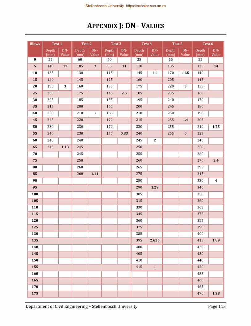
Department of Civil Engineering – Stellenbosch University Page 113
APPENDIX J: DN - VALUES
Blows Test 1 Test 2 Test 3 Test 4 Test 5 Test 6
Depth (mm)
DN- Value
Depth (mm)
DN- Value
Depth (mm)
DN- Value
Depth (mm)
DN- Value
Depth (mm)
DN- Value
Depth (mm)
DN- Value
0 55 60 40 35 55 55
5 140 17 105 9 95 11 110 135 125 14
10 165 130 115 145 11 170 11.5 140
15 180 145 125 160 205 145
20 195 3 160 135 175 220 3 155
25 200 175 145 2.5 185 235 160
30 205 185 155 195 240 170
35 215 200 160 200 245 180
40 220 210 3 165 210 250 190
45 225 220 170 215 255 1.4 205
50 230 230 170 230 255 210 1.75
55 240 230 170 0.83 240 255 0 225
60 240 240 245 2 240
65 245 1.13 245 250 250
70 245 255 260
75 250 260 270 2.4
80 260 265 295
85 260 1.11 275 315
90 280 330 4
95 290 1.29 340
100 305 350
105 315 360
110 330 365
115 345 375
120 360 385
125 375 390
130 385 400
135 395 2.625 415 1.89
140 400 430
145 405 430
150 410 440
155 415 1 450
160 455
165 460
170 465
175 470 1.38
Stellenbosch University https://scholar.sun.ac.za

Department of Civil Engineering – Stellenbosch University Page 114
Stellenbosch University https://scholar.sun.ac.za