german monetary history in the first half of the twentieth … · 2015-01-29 · german monetary...
TRANSCRIPT

German Monetary Historyin the First Half of theTwentieth Century
Robert L. Hetzel
At the end of 1998, the German Bundesbank turned over the adminis-tration of monetary policy to the European Central Bank (ECB). Inthe years between World War I and 1998, the Bundesbank had come
to embody the modern central bank. What history did Germany traverse tomake possible the creation of such an institution? And how does that historyhelp us define a modern central bank?
Today, a central bank chooses one of two objectives. It may target eitherthe exchange rate or domestic economic conditions, including the inflationrate. In either case, the central bank is the unique institution charged withcontrolling the chosen objective. Such control relies exclusively on the centralbank’s management of its own balance sheet. In particular, the central bankcontrols its liabilities (the monetary base) through its asset acquisition.1
Conversely, a country with a modern central bank does not rely on govern-ment intervention in specific markets to achieve either price-level or exchange-rate objectives. If the central bank targets the exchange rate, the country doesnot rely on exchange controls, multiple exchange rates, tariffs, quotas, or other
This history will be continued in a related article, to appear in a future issue of the EconomicQuarterly. It will consider how Germany came to define stability of the mark in terms of itsinternal value (price level) rather than external value (exchange rate). It will also explain thereasons for the creation of the European Monetary System and its successor, the EuropeanMonetary Union, and review the political process that led to the creation of the ECB. Theauthor gratefully acknowledges helpful comments from Michael Dotsey, Martin M. Fase, An-dreas Hornstein, Thomas Humphrey, Jeffrey Lacker, Joachim Scheide, and Alexander Wolman.The views expressed in this article are those of the author and should not be attributed tothe Federal Reserve Bank of Richmond or to the Federal Reserve System.
1 Central banks exercise this control indirectly through use of an overnight bank rate as apolicy variable. This rate is a market rate. The need to control money creation imposed by theneed to control inflation disciplines the central bank to respect the role the interest rate plays asa price in the price system.
Federal Reserve Bank of Richmond Economic Quarterly Volume 88/1 Winter 2002 1
2 Federal Reserve Bank of Richmond Economic Quarterly
administrative measures. If the central bank targets the inflation rate, the coun-try does not rely on wage and price controls, guideposts, antitrust actions, orspecial intervention into the wage and price-setting decisions of firms. A mod-ern central bank does not in general allocate credit either through subsidizedlending at the discount window or quotas on the credit that individual bankscan extend.
This article reviews German monetary history in the first half of the twenti-eth century, employing the theme that the evolution of the concept of a moderncentral bank required popular support for a free market.2 It summarizes threeepisodes: hyperinflation in the twenties, deflation in the early thirties, andthe currency reform of 1948. Inflation and deflation accompanied the eco-nomic instability of the first and second episodes, respectively. In each case,free enterprise lost public support. The third episode inaugurated a period ofeconomic and monetary stability, during which free enterprise again becameacceptable.
1. HYPERINFLATION IN THE WEIMAR REPUBLIC
In 1913, total currency in Germany amounted to just 6 billion marks. InNovember 1923 in Berlin, a loaf of bread cost 428 billion marks and a kilogramof butter almost 6,000 billion marks. From the end of World War I until 1924,the price level rose almost one trillionfold.3 The economic cause of thishyperinflation was the monetization of public and private debt by Germany’scentral bank, the Reichsbank.4 The political cause lay in the inability of afragile democracy to impose the taxes necessary to pay war reparations.5
Reparations and Budget Deficits
Germany entered World War I believing that the war would be like the Franco-Prussian War of 1870–1871 and that the government would be able to financea short war by issuing bonds, which a defeated France would redeem in gold(Marsh 1992, 77). In fact, the combatants devoted half of their economicoutput to the fighting. The central government in Germany, which did notimpose income taxes, financed the war almost completely by issuing debt.
2 An intellectually kindred exercise is Humphrey (1998). He traces the historical relationshipbetween proponents of the quantity theory and free markets on one hand and anti-quantity theoristsand mercantilists on the other. The quantity theory explains how governments can control the pricelevel or trade balance without direct intervention in markets.
3 The figures are from Webb (1989, 3) and Bresciani-Turroni (1937, 25).4 Among others, Bresciani-Turoni (1937), Keynes (1923), Cagan (1956), and Webb (1989)
present this quantity theory view.5 Among others, Holtfrerich (1986) and Webb (1989) present this view. The earliest criticism
of the punitive character of the Versailles treaty by an economist is Keynes (1919).

R. L. Hetzel: German Monetary History 3
With the deficits that followed the end of the war, the Reich’s debt amountedto half of national wealth. Interest on the debt amounted to four times theReich’s 1913 revenues.6
At Versailles, the victorious Allies imposed a punitive settlement on Ger-many. They stripped Germany of its colonies and Alsace-Lorraine. The Ver-sailles treaty required that Germany pay for the damages caused by the warwithout stipulating an upper limit. France in particular demanded heavy repa-rations, embittered by the appalling human cost of retaking Alsace-Lorraine.
In May 1921, in the London Ultimatum, theAllies set an aggregate amountfor reparations of 132 billion gold marks. However, the Ultimatum allowedthe Reparations Commission to demand interest on the unpaid amount when itjudged that German finances had recovered. Uncertainty about the total repa-rations payments and the disincentive to run fiscal surpluses that uncertaintycreated for Germany probably weighed even more heavily than the huge mag-nitude of the total. Foreign lenders then found it difficult to assess Germany’scredit worthiness (Holtfrerich 1986, 143, 145, 154).
Because of differing valuations placed on payments in kind, it is difficultto measure the reparations Germany actually paid. Holtfrerich (1986, 151)compares various estimates and concludes that for the years 1919 through1922, Germany paid 10 percent of its national income in reparations. Webb(1989, 106) arrives at a similar number, which amounted to 80 percent ofGermany’s exports. Holtfrerich (1986, 153) points out that, as a fraction ofnational income, reparations equalled the amount of government expenditureat all levels in the prewar period.
Holtfrerich (1986, 153) argues that Germany could not have raised throughdirect taxation the amounts necessary “to effect a foreign transfer regardedfrom the outset as beyond fulfillment, unjust and indeed morally reprehensibleby almost the entire population.” He explains the resort to an inflation tax byquoting Friedrich Bendixen, a Hamburg bank director:
Only in taxation do people discern the arbitrary incursions of the state;the movement of prices, on the other hand, seems to them sometimesthe outcome of traders’ sordid machinations, more often a dispensationwhich, like frost and hail, mankind must simply accept. The statesman’sopportunity lies in appreciating this mental disposition. (153)
Unable to cover its expenditures through explicit taxes, the German gov-ernment ran deficits exceeding 50 percent of its expenditures from 1919through 1923 (Holtfrerich 1986, 173). Reichsbank purchases of governmentdebt made the printing press the ultimate source for funding these deficits.7
6 These figures are from Holtfrerich (1986, 102, 109, 126).7 Keynes (1923, Chapter 2) explains inflation as a tax.

4 Federal Reserve Bank of Richmond Economic Quarterly
Holtfrerich (1986, 152) reproduces figures of Arnd Jessen showing that, asa proportion of government expenditures, the yield of the inflation tax alsoamounted to about 50 percent. In the years 1919, 1920, 1921, and 1922, rev-enue from the inflation tax respectively amounted to 62, 53, 43, and 43 percentof government revenue.
A Chronology of Inflation
Although money creation ultimately caused German inflation, expectationsabout the ability of the government to achieve ultimate fiscal balance de-termined inflation’s timing (Webb 1989). The foreign and domestic publicwillingly purchased new debt issues when it believed that the governmentcould run future surpluses to offset contemporaneous deficits. When it didnot, the debt presented to the Reichsbank rose. Foreign speculative capitalinflows ceased, the exchange rate depreciated, and inflation rose.
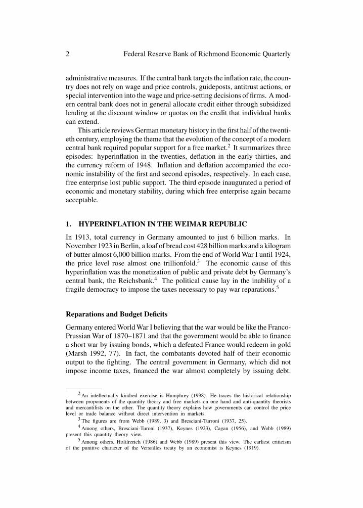
Inflation exacerbated the government deficit by reducing tax revenue. Be-cause the government levied taxes in nominal terms, the elapsed time betweenassessment and collection destroyed their real value (Bresciani-Turroni 1937,66; Sargent 1993, 69). Figure 1 reveals the pattern of an inflation driven byfiscal fears. It shows the wholesale price index with the periods demarcatedas by Webb (1989, 5).
At the end of the war, the fiscal situation was gloomy. In November 1918,a worker revolution overthrew the Kaisertum. Widespread, paralyzing strikesoccurred. The new government issued debt to obtain the food supplies andfunds for demobilization that were necessary to limit social unrest (Marsh1992, 79). The government subsidized food, coal, and employment in therailway and postal systems to prevent a second worker revolt.
The new government’s concern was valid, for it was indeed possible thatfiscal restraint would raise unemployment and set off a Bolshevik revolution(Ferguson and Granville 2000, 1063–65; James 1999, 18). The price level rosefrom the end of the war until early 1920. By February 1920, the wholesaleprice level had risen to 17 times its 1913 level. According to Webb (1989, 52),this rise reduced the real value of the nominal government debt outstandingin October 1919 (172 billion marks) to a value consistent with future budgetbalance. The political situation stabilized in March 1920 with the failure ofthe Kapp Putsch.
The price level steadied after March 1920.8 Minister of Finance MatthiasErzberger implemented tax reforms that brought Germany close to achievingfuture budget balance. Although the budget remained in deficit, tax revenues
8 Regarding this paragraph and the next, see Webb (1989, 54–60) and Holtfrerich (1986,301–11).
R. L. Hetzel: German Monetary History 5
Figure 1 Monetary Base and Wholesale Price Index
Notes: Data normalized with 1913 equal to 1. Observations are the natural logarithm.The figure uses the data in Diagram 4 in Holtfrerich (1986). The monetary base is cashin circulation plus commercial bank deposits at the Reichsbank.
were rising steadily. Given stable real expenditures, growth in the econ-omy would have increased revenues and balanced the budget. These calcu-lations depended upon maintenance of the current level of reparations, whichamounted to 2.24 billion marks in the 12-month period ending 21 June 1920.
However, in the London Schedule of May 1921, the Allies threatened tooccupy the Ruhr unless Germany transferred 4 billion marks annually andmade additional payments as its economy grew. The Reichstag refused to im-pose additional taxes, and inflation rose when the prospect of ultimate budgetbalance receded. As inflation rose, collection lags in the tax system reducedreal revenues. In October 1921, the Allies further weakened the politicalstanding of the German government by annexing Upper Silesia to Poland.
Only the United States was in a position to broker a compromise, for itcould have forgiven war debts owed it by France and Britain in return formoderation of their reparations demands. But the United States retreated intoisolationism. Contradictorily, Allied governments made it hard for Germanyto run the surplus on its external trade account that was necessary to pay repa-rations by imposing high duties on its exports. Many Germans adopted thefatalistic attitude that German economic ruin would be necessary to demon-strate the injustice of reparations. They contended that only when the Allies

6 Federal Reserve Bank of Richmond Economic Quarterly
scaled back demands for reparations could Germany bring order to its domesticfinances.
To support their case, they argued that the reparations caused inflation:The purchase of foreign exchange to make reparations payments depreciatedthe mark.9 In turn, the depreciation of the mark raised internal prices. An endto the monetization of government debt without a settlement of the reparationsissue would leave unchecked both the depreciation of the mark and domesticinflation. Because the government would still have to maintain subsidies, itwould become bankrupt. Rudolf von Havenstein, the head of the Reichsbank,said, “So long as the reparations burden remains, there is no other meansto procure the necessary means for the Reich than the discounting of ReichTreasury notes at the Reichsbank” (Feldman 1997, 445).10
Inflation became hyperinflation with the assassination of foreign ministerWalther Rathenau in July 1922 by right-wing reactionaries. Capital flightspurred mark depreciation, which exacerbated domestic price increases. Theresulting fall in the purchasing power of the mark created a liquidity crisis.To deal with this crisis, industrialists argued for the rediscounting of bills ofexchange at the Reichsbank. Georg Bernhard, an influential newspaper editorand member of the Reich Economic Council, argued that “There is only onesource of money in Germany left, the Reichsbank. . . . It is thus absolutelycorrect that we create commercial bills; then the Reichsbank can issue money”(Feldman 1927, 450). In the second half of 1922, the Reichsbank began todiscount significant numbers of private bills (Webb 1989, 28).
Karl Helfferich, finance minister during World War I, said that if theReichsbank ceased “the printing of notes. . . all national and economic lifewould be stopped.”11 Hjalmar Schacht (1927), later the Reichsbank presi-dent, wrote:
In 1923 there were engaged on the production of notes for the Reichs-bank. . . 1,783 machines. . . . [E]ven with assistance on so vast a scale the
9 See references in Bresciani-Turroni (1937, Chapter II), especially pages 77 to 82.10 The argument is a mixture of economic fallacy and political insight. As a matter of positive
economics, a depreciation of the mark on the foreign exchanges could not in and of itself producea significant rise in the domestic price level. A rise in the price level would have reduced the realmoney holdings of the German public. The attempt by the German public to restore its monetarypurchasing power through a reduction in expenditure would have reversed the rise in the domesticprice level (apart perhaps from an amount relecting a reduction in desired real money holdings asa consequence of feeling poorer due to the mark depreciation).
From a political perspective, however, without an end to the reparations, the problems ofachieving fiscal balance were, if not insupurable, at least extremely difficult. If the Reichsbank hadnot monetized debt, the outstanding debt would have grown more rapidly. The effective default onexisting debt that came through inflation might then have occurred sooner and explicitly throughan actual default. In this sense, the reparations forced the Reichsbank into a situation whereinflationary finance appeared to be the only politically feasible option.
11 Cited in Bresciani-Turroni (1937, 81).

R. L. Hetzel: German Monetary History 7
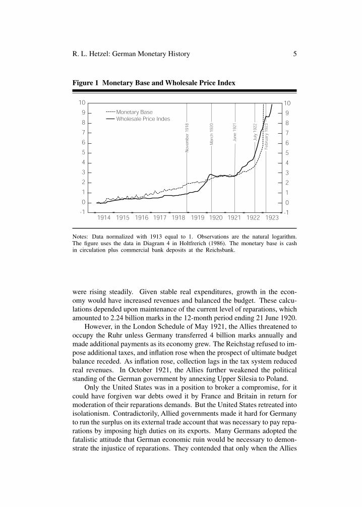
Figure 2 Industrial Production
Notes: Data normalized with 1928 equal to 100. Observations are the natural logarithm.The figure reproduces Diagram 4 in Holtfrerich (1986).
Bank was not in a position to supply the business world with a sufficiencyof notes. (105)
In fact, the high rate of inflation made holding money extraordinarilycostly. German moneyholders responded rationally by reducing the realamount of marks they held.12 The minimal real purchasing power of marksmade money appear scarce. That scarcity rationalized the demands of the in-dustrial class for the Reichsbank to continue discounting its commercial paperat a discount rate of 6 percent. In this way, industrialists obtained costlesslythe revenues from the taxing powers (seigniorage) that money creation grantedto a central bank.
France never confronted the inherent contradictions in its policy towardGermany. It wanted a weak German economy incapable of supporting remil-itarization, and it wanted the payment of reparations, which required a strongGerman economy. On 11 January 1923, France occupied the Ruhr when Ger-many failed to make in kind deliveries of coal. Germany responded with apolicy of passive resistance. With government support, workers in the Ruhrwent on strike to prevent France from obtaining the region’s coal and steel.
12 They achieved the reduction in the purchasing power of the mark by increasing the pricelevel in excess of the amount of paper marks issued.

8 Federal Reserve Bank of Richmond Economic Quarterly
Without coal, German railroads could not run, and without railroads theGerman economy could not run. Figure 2 shows the decline in output precip-itated by the Ruhr occupation. Germany had to import coal. The governmentalso had to pay striking workers, in part, it believed, to prevent them fromjoining the Communist movement and starting a Bolshevik revolution. As thegovernment deficit widened to 22 percent of net national product, the moneystock soared (Ferguson and Granville 2000, 1068).13 By year-end 1922, themark-dollar exchange rate had fallen from its prewar level of 4.2 to 1 to 1,500to 1. By the end of November 1923, it had fallen to 4,200,000,000,000 to 1.
End of the Hyperinflation
On 20 November 1923, Germany ended inflation by pegging the mark’s for-eign exchange value at its prevailing value of 4,200 billion marks to the dollar.14
What made monetary reform credible to the German public?As background, note a characteristic of twentieth-century monetary re-
forms that ended hyperinflations (for example, in Argentina in 1991).15 At thetime of a reform, the economy in question is using a stable currency as thestandard of value, often the dollar, rather than the domestic currency. In hy-perinflations, individuals set prices in dollars and then use the dollar exchangerate to convert prices to domestic currency equivalents. The domestic moneyserves only as a token currency for small transactions. One prerequisite fora successful monetary reform is to make credible the maintenance of a fixeddollar exchange rate, which will reestablish individuals’faith in the purchasingpower of domestic currency.
In 1923, “German society was moving massively to disown the papermark” (Feldman 1997, 691). The German economy largely indexed (“val-orized”) transactions to maintain their real value. One example was a bankproposed by Hans Luther and Rudolf Hilferding (Food and Finance Ministers,respectively) that would issue a “rye” mark, that is, a deposit redeemable inrye. The bank came into existence on 15 November 1923 as the Rentenbank,but with a rentenmark deposit convertible to gold at the prewar value. The
13 Webb (1989, Chapters 2 and 3) provides a careful account of the interaction between thefiscal system and inflation. Inflation reduced the revenue that government raised because it vitiatedthe real value of taxes, which the government set in nominal terms but collected with a delay.If Germany had had a period of price stability or if it had indexed its tax system, it could havebalanced its budget. (The wealthy opposed indexing because it would have prevented inflationfrom reducing the real value of their tax liability.) In the absence of inflation, the tax reformsthe government passed might have raised sufficient revenue to cover domestic expenditure andreparations payments. However, the government faced an incessant set of domestic and externalpressures (such as French demands to pay immediate cash reparations). As a result, it never had aninterval of time during which it could have stopped inflation by meeting its expenditures withoutprinting money (Webb 1989, 42–43).
14 For a brief account of the November 1923 monetary reform, see Humphrey (1980).15 For other examples, see Bruno et al. (1988).

R. L. Hetzel: German Monetary History 9
new bank had strict limits on the credit it could extend to the private sectorand to the government and met with “astounding success” (Holtfrerich 1986,316).
The actual breakdown of German economic life came about because ofinterventions by the German government to maintain the paper mark as themedium of exchange. Holtfrerich (1986, 313) writes of hyperinflation Ger-many, “The economy had already largely turned over to a foreign, hard-currency standard. . . . The crisis arose out of the reluctance of the Reich topermit business to employ foreign means of payment in domestic transactionsas desired; indeed the Reich could not permit the practice. . . as long as inflationremained as a ‘tax’ source.”
Although the government ignored the price setting of the large industrialcartels, it imposed price controls on professionals and the retail trades toprevent “profiteering.” Rent control destroyed the wealth of small propertyowners. Because farmers could not borrow using an indexed value of land ascollateral, they could not obtain fertilizer (Feldman 1997, 681–84). “Becausethe farmers were already refusing to accept the currency. . . Germany faced theimminent danger of hunger revolts” (Feldman 1997, 693).
Bresciani-Turroni offers two observations helpful for understanding theGerman reform. First, “At the beginning of the inflation. . . the public stilldid not understand the phenomenon of monetary depreciation” (Bresciani-Turroni 1937, 430). However, by the end, the public associated inflation withthe money issues of the Reichsbank. Everyone knew at that point that an end toinflation would require the Reichsbank to limit monetary emission to whateverwas needed to maintain the new mark-dollar exchange rate. Second, hyperin-flation threatened imminent economic and social collapse. Holtfrerich (1986,312), citing Schacht, writes “Plundering and riots were a daily occurrence,”and Bresciani-Turroni (1937, 336) cites Luther, “The effective starving of thetowns and the impossibility of continuing economic activities on the basis ofthe paper mark was so obvious in the days preceding November 16th that adissolution of the social order must have been expected almost from hour tohour.”
The 1923 reform worked because there was political consensus that it hadto work. The economic disruption produced by the combination of hyperinfla-tion and government attempts to force continued use of the mark had pushedGermany to the edge of social disintegration. Revolts, including Hitler’s beer-hall Putsch and attempted March on Berlin on 9 November 1923, challengedthe survival of the government. A social and political consensus emerged thatthe Reichsbank had to maintain the dollar-mark exchange rate. Faced withchaos, Germany took steps to restore order.
In this changed environment, the Reichsbank ceased monetizing govern-ment debt. The amount of treasury bills held by the Reichsbank went from

10 Federal Reserve Bank of Richmond Economic Quarterly
190,000,000 trillion marks in mid-November to zero by year-end (Marsh 1992,83). Finance minister Hans Luther balanced the budget through emergencytax decrees and budget cuts. Germany declared an end to the policy of pas-sive resistance opposing the Ruhr occupation and ceased payments to strikingworkers in the Ruhr. Negotiations between Germany and the Allies beganthat led to the 1924 Dawes Plan rescheduling of reparations (Ferguson andGranville 2000, 1078; Yeager 1981, 57).
The final test that established the credibility of the Reichsbank occurredin April 1924. When the dollar value of the mark weakened, the Reichsbankdrastically restricted credit. S. Parker Gilbert, Agent General for ReparationsPayments, later cabled George Harrison, governor of the Federal Reserve Bankof New York:16
[The Reichsbank’s] policy resulted in [a] check to [the] increase ofReichsbank credit and circulation, development of excess of exportsover imports, liquidation of heavy commodity stocks accumulated duringinflation, decline in commodity prices, and large failures of many firmsestablished during inflation. Rates for month[ly] money rose from 30 to80 percent but later declined rapidly.
Discrediting Capitalism
Ferguson and Granville (2000, 1084) write, “By discrediting free markets, therule of law, parliamentary institutions, and international economic openness,the Weimar inflation proved the perfect seedbed for national(ist) socialism.”The Weimar inflation produced arbitrary redistributions of income that dis-credited the market economy. As a class, the wealthy were the main losersbecause they held most of the mark-denominated financial wealth. Pension-ers, bondholders, and rentiers lost everything. Laws against indexation andprofiteering hurt merchants. Workers who were protected by labor unionspreserved their real wages.17
Keynes has described how inflation destroys the social foundation of amarket economy:
By a continuing process of inflation, governments can confiscate, secretlyand unobserved, an important part of the wealth of their citizens. Bythis method they not only confiscate, but they confiscate arbitrarily; and,
16 S. Parker Gilbert memo to George Harrison, “Reichsbank Credit Policy,” 22 July 1931,Harrison Papers. The Harrison Papers are at the Federal Reserve Bank of New York and ColumbiaUniversity. Gilbert refers to the description of the episode on page 162 of Schacht’s book, Stabi-lization of the Mark.
17 These generalizations come from Holtfrerich (1986, Chapter 8) and Webb (1989, Chapter5).

R. L. Hetzel: German Monetary History 11
while the process impoverishes many, it actually enriches some. . . . Thoseto whom the system brings windfalls. . . become profiteers. (1919, 148–49)
To convert the business man into a profiteer is to strike a blow atcapitalism, because it destroys the psychological equilibrium which permitsthe perpetuance of unequal rewards. (1923, 24)
Lenin was certainly right. There is no subtler, no surer means of over-turning the existing basis of society than to debauch the currency. Theprocess engages all the hidden forces of economic law on the side ofdestruction, and does it in a manner which not one man in a millionis able to diagnose. . . . By combining a popular hatred of the class ofentrepreneurs with the blow already given to social security by the violentand arbitrary disturbance of contract. . . governments are fast rendering im-possible a continuance of the social and economic order of the nineteenthcentury. (1919, 149–50)
Popular resentment concentrated on speculators. When Germans soldtheir family heirlooms to survive, they blamed the middlemen who organizedthe sales. A fictional character called Raffke, created by cabaret songwriterKart Tucholsky, embodied the culturally ignorant person made rich from profi-teering (Feldman 1997, 553). Bresciani-Turroni (1937, 328) would later writeof “the poverty of certain German classes during the inflation which contrastedwith the foolish extravagance and provocative ostentation of inflation profi-teers.”
Nationalist resentment targeted all foreigners but most especially the mi-nority within reach—Jews. Hitler railed against the “Jewification of the econ-omy” (Feldman 1997, 780, 575). On 5 November 1923, the government raisedthe price of bread to 140 billion marks, and in response, crowds plunderedstores and attacked Jews. In July 1922, the British Consul in Frankfurt wrote:
[T]he educated classes, deprived, in a great majority of cases, of the rightto live and bring up their families in decency, are becoming more andmore hostile to the Republic and open in their adhesion to the forces ofreaction. Coupled with this movement, a strong and virulent growth ofanti-Semitism is manifest. (Feldman 1997, 449)
Germans wanted a world where wealth resulted from hard work, not fi-nancial transactions. According to Feldman (1997), Germans desired a returnto a world where
the public good should take precedence over private gain. . . . It was not onlyHitler who appealed to these sentiments. . . . [I]nflation. . . caused the Repub-lic to be identified with. . . violations of law, equity and good faith. . . . Noless offensive. . . was the sense that there had been a misappropriation ofspiritual values. (657–58)

12 Federal Reserve Bank of Richmond Economic Quarterly
2. WORLD DEPRESSION
Germany ended hyperinflation and restored social order with its commitmentto the gold standard. The November 1923 stabilization program commit-ted Germany to exchange 1,392 reichsmarks for a pound of gold. However,German economic stability then became dependent upon the stability of theinternational gold standard. Starting in 1928, the deflationary monetary poli-cies of two of the largest adherents to the gold standard, France and the UnitedStates, forced deflation and economic depression on Germany. Short-run sal-vation led to longer-run doom. The following section explains the fragility ofthe reconstructed gold standard.
Reviving the International Gold Standard
In 1920, Britain legislated a return to the gold standard at the prewar parityto take effect at the end of a five-year period. Britain based its decision inpart on the assumption that gold flows to the United States would raise pricelevels there and limit the domestic deflation needed to reestablish the prewarparity (Rothbard 1996, 8). In fact, the United States sterilized gold inflowsto prevent a rise in domestic prices. In the 1920s, the Federal Reserve heldalmost twice the amount of gold required to back its note issue (Yeager 1976,333). Britain then had to deflate to return to gold at the prewar parity.18
After the war, France had counted unrealistically on German reparationsto balance its budget. When they did not materialize, it used inflation asa tax to finance expenditures. In 1926, France pulled back from the brinkof hyperinflation. Unlike Britain, in France inflation had put the old parityhopelessly out of reach. As a consequence, France returned to gold at a paritythat undervalued the franc. Scarred by its experience with inflation, Francesterilized gold inflows to prevent a rise in prices.
Allied war debts and reparations added to the inherent fragility of an inter-national gold standard programmed for deflation. They required the transferof resources from Germany to France and England and then from these coun-tries to the United States. To accomplish these transfers, Germany wouldhave had to run a trade surplus toward France and Britain. In turn, France andBritain would have had to run a trade surplus toward the United States. Inthe protectionist environment of the 1920s, that trade pattern was politicallyunacceptable. Only capital outflows from the United States made the systemwork (Yeager 1976, 333; Holtfrerich 1989, 151).19
18 The prewar dollar-pound exchange rate was 4.86. After the war, in November 1920, thevalue of the pound fell to a low of 3.44. The British price level then had to fall commensuratelyto validate the former gold standard exchange rate of 4.86.
19 Eichengreen (1995, 224) calculated that most of the $2 billion in reparations paid byGermany between 1924 and 1929 went to the United States for payment of Allied war debts.

R. L. Hetzel: German Monetary History 13
World Deflation
By the end of 1927, it appeared that Europe had successfully returned to thegold standard. However, in 1928, the Federal Reserve initiated a restrictivemonetary policy to stop stock market speculation. In 1920 and 1921, a float-ing exchange rate had insulated Germany from deflationary U.S. monetarypolicy. In those years, German industrial production rose 46 and 20 percent,respectively. In contrast, in Britain, whose commitment to return to the goldstandard at the prewar parity overvalued its exchange rate, industrial produc-tion fell 32 percent in 1920.20 At the end of the decade, a revived internationalgold standard transmitted U.S. deflation to Germany.
In the 1920s, capital had flowed into Germany. That is, Germany exportednot only goods, but also IOUs. When the Federal Reserve System beganraising interest rates in 1928, those capital inflows lessened. Germany thencould not use funds gained from capital inflows to pay its reparations, butinstead had to run a trade surplus to gain the needed funds. The price levelin Germany had to fall to make its exports more attractive to the rest of theworld. By the last half of 1929, foreign debt issued in New York was lessthan a third of its 1927 level (Chandler 1958, 456). “Net portfolio lendingby the United States declined from more than $1000 million in 1927 to lessthan $700 million in 1928 and turned negative in 1929” (Eichengreen 1995,226).21
As a result, in 1928 U.S. financial markets began attracting gold from Eu-rope.22 Foreign central banks had to raise their domestic interest rates to offsetgold losses. The Federal Reserve Bulletin (November 1930, 655) talked about“Money rates abroad, which had been kept up largely to protect the reserves offoreign countries against the attraction of speculative and high-money condi-tions in the United States.” George Harrison, governor of the Federal ReserveBank of New York, informed Secretary of the Treasury Andrew Mellon that“our high money rates. . . continue to act as a pressure upon all the Europeanbank reserves.”23 At the same time, France, with its undervalued franc, alsoabsorbed gold from the rest of the world. In 1928 and the first half of 1929,France absorbed 3 percent of global gold reserves (Eichengreen 1995, 216).
America then returned the funds to Germany through capital flows. Not until 1929 did reparationspayments exceed those capital flows.
20 The figures are from Holtfrerich (1986, Table 38).21 Eichengreen (1995, 226) also documents the corresponding decline in German bond flota-
tions in New York.22 From August through December 1928, the United States imported $44.5 million in gold;
in 1929, $120 million; in 1930, $278 million; and from January through September 1931, $336million (valued at $20.67 per fine ounce). Data are from Table 156, “Analysis of Changes inGold Stock of United States, Monthly, 1914–1941,” Board of Governors (1976). Also in 1929,Germany’s scheduled reparations payments rose.
23 Harrison memo, “Conversation over the telephone with Secretary Mellon,” 29 April 1929,Harrison Papers.
14 Federal Reserve Bank of Richmond Economic Quarterly
To reverse their gold outflows, other countries had to run a trade surpluswith the United States and France. Because the Fed and the Banque de Francesterilized gold inflows, those other countries had to achieve trade surplusesthrough deflation. That is, to make their goods cheaper on international mar-kets, their price levels had to fall. By creating obstacles to trade, protectionismexacerbated the extent of the required deflation.24 The gold standard becamean engine of worldwide deflation. The most visible signs of the stress of defla-tion were financial panic and widespread bank failures as depositors withdrewgold and currency from banks.
Both international and domestic considerations compelled Germany todeflate rather than abandon the gold standard. The Banking Act, createdin 1924 as part of the Dawes reparations plan, required Germany to backits currency with gold and foreign exchange reserves equal to 40 percent ofits currency. A foreign member of the General Council, set up to overseethe Reichsbank, could stop note issue if he believed gold convertibility wasthreatened (James 1999, 25).
The foreign loans from the Morgan syndicate required Germany to stayon gold. Those loans allowed Germany to finance its reparations payments.Germany also believed that adherence to the gold standard would provideit with a reputation for financial conservatism that would make credible itsefforts to renegotiate reparations obligations. Finally, and most important,seared by the memory of hyperinflation, German public opinion supportedthe gold standard. Germans associated abandonment of the gold standardwith inflation (Bresciani-Turroni 1937, 402; Eichengreen 1995, 270; James1999, 25). Politicians had difficulty supporting a possibly inflationary policywithout appearing to favor large industry and agriculture, which as debtorshad profited from the earlier inflation (Feldman 1997, 853).
The 1931 German Financial Panic
As noted above, the Reichsbank had to maintain at least a 40 percent gold cover,that is, a gold-reserves-to-note circulation ratio of 40 percent. In April 1929,with the near collapse of reparations negotiations in Paris, reserve outflowsthreatened the gold cover. In May 1929, the successful resumption of thenegotiations reestablished calm and led to the Young Plan, signed in June. InSeptember 1930, when elections gave Hitler’s party the second largest majorityin the Reichstag, gold outflows from the Reichsbank resumed; aid from aninternational consortium relieved the crisis. In May 1931, the gold cover hadrisen to a comfortable 60 percent.25
24 The U.S. Congress passed the Smoot-Hawley tariff on 13 June 1930.25 This paragraph summarizes Goedde (2000, 16–17).
R. L. Hetzel: German Monetary History 15
Any lasting restoration of investor confidence in the mark’s gold paritywould require settlement of the reparations issue.26 Investors worried whetherGermany could finance reparations payments in the absence of continued cap-ital inflows. They also worried about the political instability within Germanycaused by reparations. Right-wing parties demanded that Germany renouncereparations. The Bruening government had been unable to form a parliamen-tary majority since July 1930. Chancellor Bruening dismissed the Reichstagand governed without it.
At the beginning of June 1931, the Reichsbank again began to lose gold.27
This worsening in the German balance of payments ultimately occurred at thistime because the deflationary pressure of U.S. monetary policy intensified.The U.S. money stock M2 had declined only 2 percent in 1930. In 1931Q1and 1931Q2, it fell at an annualized rate of 6.3 and 6.7 percent, respectively.In 1931Q3, M2 declined at an annualized rate of 11.3 percent (Friedman andSchwartz 1963).28
Bank failures in Austria and Hungary were the immediate source of thefinancial panic in Germany. The first of these was the failure of the Aus-trian Credit-Anstalt bank in mid-May 1931, after which Austria suspendedgold convertibility and allowed its currency to depreciate. Because foreignersheld half of German bank deposits, financial stability required that foreigninvestors retain confidence in the maintenance by Germany of its gold parity(Eichengreen 1995, 272). Only American leadership could have achieved thatresult.
On 20 June 1931, President Hoover proposed a one-year moratoriumon reparations and Allied debt payments. Financial markets worldwide re-sponded positively (Eichengreen 1995, 277). However, French ill will towardGermany delayed the negotiations until a debt moratorium was too late to help.French reluctance to agree to the Hoover moratorium made investors nervous.That nervousness caused the financial panics in Austria and Hungary to jumpthe border to Germany.29
26 See Norman telephone conversation with Harrison, 18 June 1931, Harrison Papers. See alsoShepard Morgan, “Memorandum on German Short-Dated Debt Reduction,” 6 July 1931, HarrisonPapers.
27 Eichengreen (1995, Chapter 9) contains a chronological account of the 1931 financial crisis.28 An alternative view is that the 1931 financial crisis originated as a banking crisis. See
references in Balderston (1994). According to this view, depositors came to see German banksas insolvent. When they withdrew their funds, a foreign exchange crisis developed. On the basisof an examination of deposit withdrawals at German banks, Balderston (1994) disputes this view.(See also Goedde [2000, 22].) He argues that the banking crisis emerged from a foreign exchangecrisis. In his view, foreign depositors withdrew funds from German banks as political developmentsmade a negotiated settlement of reparations less likely. Pontzen (1999, 79) backs Balderston’s view.He points out that capital outflows abroad set in before withdrawals by domestic depositors. Healso points to foreign investor nervousness caused by a more aggressive stance toward reparationsby the German government.
29 Cablegram Dreyse to Harrison, 11 July 1931, Harrison Papers.

16 Federal Reserve Bank of Richmond Economic Quarterly
Figure 3 The Inverse of Velocity and the Interest Rate 1925–1939
Notes: The interest rate is “Day-to-day money” in “Table 172—Money Rates in SelectedForeign Countries” in Board of Governors Banking and Monetary Statistics (1943). Ve-locity is nominal GNP (the product of Real GNP and the GNP Deflator) divided bymoney. See Table 2.
The appendix, “The Federal Reserve Bank of New York and the Reichs-bank during the 1931 Crisis,” provides an account of these events recordedin memos by Governor Harrison of the New York Fed. Central banks hadcooperated to maintain the gold standard in the twenties. Walter Bagehot, aBritish economist, had expounded the lender-of-last-resort principle of lend-ing freely at a high interest rate in a financial crisis (Bagehot 1873). Theseprecedents suggested that the New York Fed, the Bank of England, and theBanque de France would lend to the Reichsbank. Had they done so, it ispossible that monetary contraction and the fall in the German price level nec-essary to improve Germany’s trade balance could have occurred in an orderlyfashion. However, as a condition for a loan, the New York Fed required thatthe Bundesbank cease lending to commercial banks. The Reichsbank’s com-pliance precipitated the collapse of its banking system, and the New York Fedthen failed to come through with a loan.
Between 1926 and 1932, the Reichsbank maintained short-term interestrates at around 6 percent (Figure 3).30 Figure 4 shows that significant deflation
30 The initial high value of 9 percent in 1925 is a carryover from the very high rates neededin 1924 (45 percent in April 1924) to maintain the new gold parity for the mark (James 1999,27).

R. L. Hetzel: German Monetary History 17
Figure 4 GNP Deflator
Notes: See Table 2.
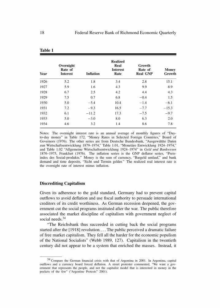
began in 1929 and continued through 1932. Despite this deflation, the Reichs-bank kept market interest rates high. Table 1 shows the realized real rate ofinterest—the market rate minus actual inflation. This series rose moderatelythrough 1929 and dramatically in the years 1930, 1931, and 1932.31
Monetary contraction allowed the Reichsbank to maintain high real ratesof interest. Given the stability of monetary velocity (Figure 3), monetarycontraction required a decline in nominal output (Figure 5).32 Real outputpeaked in 1928 and then fell 16 percent through 1932. Only in 1933 didoutput begin a modest recovery (Figure 6 and Table 2).33
31 The relevant series is the real rate of interest, which is the market rate of interest minusexpected inflation. For the United States, Hamilton (1992, 172) estimates that in the Great De-pression the public forecast about half of actual inflation. If the public in Germany forecast anysignificant fraction of the actual deflation, then real rates of interest were extraordinarily high inthe years 1930, 1931, and 1932.
32 Figures 3 and 5 show that after 1937 money rose with no corresponding rise in prices(velocity fell). This divergence is probably an artifact due to price controls. Official price indicesdid not measure the deterioration in the quality of goods (James 1999, 35).
33 For the view that the Great Depression resulted from nonmonetary rather than monetarycauses see Fisher and Hornstein (2001).
18 Federal Reserve Bank of Richmond Economic Quarterly
Table 1
RealizedOvernight Real Growth
Rate of Interest Rate of MoneyYear Interest Inflation Rate Real GNP Growth
1926 5.2 1.8 3.4 2.8 15.1
1927 5.9 1.6 4.3 9.9 8.9
1928 6.7 2.5 4.2 4.4 4.3
1929 7.5 0.7 6.8 −0.4 1.5
1930 5.0 −5.4 10.4 −1.4 −6.1
1931 7.2 −9.3 16.5 −7.7 −15.3
1932 6.1 −11.2 17.3 −7.5 −9.7
1933 5.0 −3.0 8.0 6.3 2.0
1934 4.6 3.2 1.4 8.6 7.8
Notes: The overnight interest rate is an annual average of monthly figures of “Day-to-day money” in Table 172, “Money Rates in Selected Foreign Countries,” Board ofGovernors (1976). The other series are from Deutsche Bundesbank, “Ausgewahlte Datenzun Wirtschaftsentwicklung 1879–1974,” Table 1.01, “Monetare Entwicklung 1924–1974,”and Table 1.02 “Allgemeine Wirtschaftsentwicklung 1924–1974” in Geld und Bankwesen1876–1975, Frankfurt (1976). The inflation series is the GNP deflator series, “Preis-index des Sozial-produkts.” Money is the sum of currency, “Bargeld umlauf,” and bankdemand and time deposits, “Sicht und Termin gelder.” The realized real interest rate isthe overnight rate of interest minus inflation.
Discrediting Capitalism
Given its adherence to the gold standard, Germany had to prevent capitaloutflows to avoid deflation and use fiscal authority to persuade internationalcreditors of its credit worthiness. As German recession deepened, the gov-ernment cut the social programs instituted after the war. The public thereforeassociated the market discipline of capitalism with government neglect ofsocial needs.34
“The Reichsbank thus succeeded in cutting back the social programsstarted after the [1918] revolution. . . . The public perceived a dramatic failureof free market capitalism. They fell all the harder for the economic populismof the National Socialists” (Webb 1989, 127). Capitalism in the twentiethcentury did not appear to be a system that enriched the masses. Instead, it
34 Compare the German financial crisis with that of Argentina in 2001. In Argentina, capitaloutflows and a currency board forced deflation. A street protester commented, “We want a gov-ernment that represents the people, and not the capitalist model that is interested in money in thepockets of the few” (“Argentine Protests” 2001).

R. L. Hetzel: German Monetary History 19
Table 2 German Historical Data
Year Money∗ Unemploy- Real GNP- WPI CPI Unemploy-ment GNP Deflator ment Rate
1924 978 137.3 130.8
1925 17106 636 59.7 117.9 141.8 141.8
1926 19683 2010 61.4 120.0 134.4 142.1
1927 21438 1327 67.5 121.9 137.6 147.9
1928 22369 1391 70.5 125.0 140.0 151.7 6.7
1929 22694 1899 70.2 125.9 137.2 154.0 9.0
1930 21304 3076 69.2 119.1 124.6 148.1 14.6
1931 18042 4520 63.9 108.0 110.9 136.1 22.3
1932 16288 5575 59.1 95.9 96.5 120.6 28.1
1933 16608 4804 62.8 93.0 93.3 118.0 24.4
1934 17897 2718 68.2 96.0 98.4 121.1 13.8
1935 20001 2151 74.6 98.0 101.8 123.0 10.7
1936 21609 1593 81.2 100.0 104.1 124.5 7.6
1937 23309 912 90.0 101.0 105.9 125.1 4.2
1938 28490 429 99.2 101.0 105.7 125.6 1.9
1939 37910 119 107.2 102.0 106.9 126.2 0.5
1940 48640 52 110.0 130.1 0.2
∗Equals the sum of currency and demand and time deposits.
Notes: Deutsche Bundesbank, ed. Geld und Bankwesen 1876–1975 (1976). The unem-ployment rate is from Bundesarbeitsblatt 7–8 (1997), Bundesanstalt fur Arbeit, Bundes-ministerium fur Arbeit und Sozialordnung.
appeared to be a system that allowed the strong to exploit the weak. Thedepression discredited capitalism.
Harold James (1986) writes:
It was the outbreak of the banking crisis in the summer of 1931 thatmade the German depression so severe. . . . [T]he collapse of the banksin central Europe had a major social, psychological and political impact.Capitalism appeared to have crashed with the banks, and this helped todiscredit existing political systems. (283–84)
The years following the 1923 stabilization had offered the promise of areturn to stability. The Young Plan for German reparations, adopted in prin-ciple at The Hague in August 1929, promised an end to reparations in 1988.Right-wing German parties rejected reparations and the “war guilt lie” theyrepresented (Nicholls 1968, 137). Nevertheless, in early 1930 these parties,including the Nazi party, were marginal. Their marginal status changed with

20 Federal Reserve Bank of Richmond Economic Quarterly
the spread of the depression. Under the stress of the deflation that began in1929, Germany could not keep together a political coalition capable of main-taining the democratic institutions of the Weimar Republic. Hitler was theclear beneficiary of the nationalist resentments revived by rising unemploy-ment.35 The unemployment rate averaged 28.1 percent in 1932 (Table 2).Hitler became chancellor of the government in January 1933.36
When Hitler came to power, the Reichsbank began to discount bills tofinance his public works and rearmament program. In 1936, Hitler imposeda price freeze to control inflation. He said, “Inflation is a lack of disci-pline. . . . I’ll see to it that prices remain stable. That’s what my storm troopersare for” (Feldman 1997, 855). And again, “The first cause of the stability of thecurrency is the concentration camp” (James 1999, 35). Schacht, who becameReichsbank president for the second time in March 1933, maintained the markprice of gold by imposing foreign exchange controls and barter arrangementsfor foreign trade. “Germans who settled foreign debts directly with their cred-itors were threatened with the death penalty” (Pringle 1998, 71). Germansrejected the arbitrary redistribution of wealth produced by hyperinflation andthe unemployment produced by deflation. With the discrediting of capitalism,they turned to monetary arrangements that required the detailed control ofindividual behavior by the state.
3. THE BIRTH OF THE D-MARK
Once capital controls effectively ended the gold standard, the Reichsbankwas able to finance Germany’s rearmament and war expenditures by printingmoney. Price controls created suppressed inflation. After the war ended, theAllied occupation forces maintained the price controls, and inflation continuedto be suppressed.
The currency reform of 1948 ended price controls and introduced thedeutsche mark (DM). The ensuing period of strong economic growth (theWirtschaftswunder) and the resulting monetary stability contrasted with the
35 Johnson (1998, 36) writes: “Thus Hitler and the Nazis were enabled in no small measureto seize power by demagogically exploiting popular—and populist—outrage at the banking sys-tem, the Depression, and capitalism in general. . . . Hitler’s Nazis never enjoyed significant electoralsupport—not even after hyperinflation—until the onset of the Great Depression in 1929.”
36 I am not saying that a deflationary U.S. monetary policy propagated to the world by thegold standard “caused” the rise of Hitler. An extraordinary number of factors had to fall into placeto make possible Hitler’s ascendancy. Today, nothing can undo the horrors of the first half of thetwentieth century. However, one can try to understand the near collapse of Western civilizationand the near triumph of totalitarianism. After World War I, central banks did not understandtheir responsibility for control of the price level in a fiat money regime. That ignorance allowedthe hyperinflations following World War I. Also, the newly created Federal Reserve System didnot understand how its deviation from the rules of the international gold standard could createworldwide deflation and depression. An understanding of how central banks contributed to theeconomic instability that characterized the first half of the twentieth century helps explain whatwent wrong.

R. L. Hetzel: German Monetary History 21
hyperinflation and subsequent deflation of the Weimar Republic. That contrastbred the presumption that economic and social stability required monetarystability, and this widespread presumption later created popular support forthe “stability” policy of the Bundesbank.
Price Controls and Suppressed Inflation
Despite the devastation of World War II, Germany was in a position to recovereconomically after the war. Buchheim (1999) writes:
The conditions for resuming production in western Germany were actuallyvery good. Despite the war dead, the influx of refugees and expelleessaw a sharp rise in the general population. . . . [M]any of the newcomershad been employed in industrial production occupations and had theappropriate skills. . . . [N]ew investments during the war had far exceededthe plant facilities destroyed. For this reason, West German industrialassets in 1945 were not only greater than before the war, but also moremodern. (57–58)37
However, in 1947, two years after the end of the war, industrial productionin Germany amounted to only 40 percent of its 1936 level. Price controls throt-tled German economic recovery. In other Western European countries, whichalso suffered war damage but did not have price controls, output exceeded theprewar level by 1947 (Yeager 1976, 388).
From 1936 through 1944, money (measured by currency in circulationplus total bank deposits) rose somewhat more than sixfold (Table 2). Despitethis rise in money, price controls restrained the rise in the official consumerprice index to only 14 percent from 1936 through 1944. Germany thereforeended the war with suppressed inflation. The Allies kept Hitler’s price freezein effect during the postwar occupation. Goods traded on the black marketor through barter because no one wanted to exchange goods for marks at theartificially low price level.38
Germans used nylon stockings, American cigarettes, and Parker pens forcurrency. For example, in 1945, ten cigarettes could be exchanged for 1,500grams of bread and two pairs of stockings for 1.5 pounds of butter (Hausder Geschichte).39 American soldiers could obtain those items from the PX.Germans resented the privileges that this commodity money gave Americans.General Clay, the American military governor, responded to this resentment
37 Streit (1999, 644) expresses the same view.38 Kaiserstrasse in Frankfurt was a center for the black market. Ironically, it is now the
home of the ECB, the new symbol of a valued currency.39 References to Haus der Geschichte are to the exhibits in the museum of modern German
history in Bonn.

22 Federal Reserve Bank of Richmond Economic Quarterly
by strictly enforcing the law against black market transactions (Smyser 1999,44).
Allied enforcement of price controls paralyzed the German economy. Forexample, farmers would not bring crops to market. Children died of malnour-ishment and food riots broke out (Smyser 1999, 31–32). Controls discouragedwork effort. With little effort, workers could earn enough marks to buy allthe rations allowed them by their ration cards. At the same time, the artifi-cially low wage rates did not permit workers to work long enough to buy thegoods that were available at black market prices (Buchheim 1999, 60; Hausder Geschichte).
Paradoxically, the depressing effect of the controls on economic activityseemed to assure their survival. Germans overwhelmingly saw the end of con-trols as relinquishing the certain for a frightening uncertainty. Most believedthat the disappearance of the ration cards and the minimum of sustenance thatthey assured would push the impoverished over the line into destitution (Barkand Gress 1989, 197).
Currency Reform
By early 1947, U.S. Secretary of State George Marshall understood fully thedesperate condition of Europe. He had come to believe that Stalin wouldnot accept a unified Germany except under Russian control. Marshall andErnest Bevin, the British foreign minister, concluded that the West had toreconstruct Germany without the Soviet Union (Smyser 1989, 55–56). On 5June 1947, Marshall proposed what later became known as the Marshall Plan.The United States wanted an economically viable Western Europe, whichrequired a prosperous Germany. Currency reform was a vital ingredient ofeconomic reconstruction. Germany needed a universally accepted currencyto be able to trade freely both within and across its borders.
The American economic advisers to General Clay prepared a plan forcurrency reform based on reforms in Russia and Czechoslovakia (Clay 1950,209). The reform preserved the relatively low level of controlled prices byconverting wage rates and pension payments one-for-one from reichsmarksto the new DMs. However, it eliminated the monetary overhang inheritedfrom the Third Reich by limiting the quantity of reichsmarks that could beexchanged for DMs. Under the terms of the reform, which came into effect20 June 1948, West Germans could turn in 60 reichsmarks on a one-to-onebasis. Further exchanges occurred at a ratio of ten to one. The monetaryauthority converted assets and savings deposits at a sharply reduced rate.40
40 This destruction of savings from inflation for a second time in 30 years seared into Ger-many’s collective memory an aversion to inflation that would later provide popular support for theindependence of the Bundesbank.

R. L. Hetzel: German Monetary History 23
Figure 5 Money and Nominal GNP Growth
Notes: See Table 2.
Clay (1950, 210) feared that the reform would favor the German “trendtoward socialism” by destroying the financial “savings of the little man” whilerewarding the “black market operators who had invested their huge gains inreal estate.” Therefore, the original plan included provisions for a capital levyto compensate the losers from the ten-to-one write-down of the reichsmark.However, Marshall insisted on limiting the reform to the currency exchange.
The German economic miracle began with the currency reform of June1948. When the currency reform was announced, Ludwig Erhard, economicdirector of the joint American-British Bizonal Economic Administration, de-creed the end of price controls. The day the price controls ended, goodsreturned to store shelves. With the end of controls, “euphoria engulfed mostGermans at the sight of goods and food items they could only dream aboutin the past. Bakeries miraculously produced and displayed delicious cakes;vegetables, butter and eggs appeared in abundance” (Bark and Gress 1989,201).
Industrial production in West Germany rose 25 percent within two monthsand 50 percent within six months (Buchheim 1993, 72; Marsh 1992, 173).With prices that made crops worth selling, West Germany again had enoughfood (Smyser 1999, 50). From 1948 through 1950, GDP growth in Germanyremained above 15 percent per year. In the 1950s, Germany grew at an averageannualized rate of 8 percent (Giersch et al. 1992, 2, Figure 1).

24 Federal Reserve Bank of Richmond Economic Quarterly
Figure 6 Real GNP
Notes: See Table 2.
Nevertheless, immediately after their introduction, the fate of the Erhardreforms remained in question. The currency reform carried the opprobriumof destroying the financial wealth of ordinary Germans while enhancing thetangible wealth of those holding productive capital. It thus restored the indus-trialists’ economic position, which had created envy in the Weimar Republicand Third Reich. Many Germans wanted a reintroduction of price controls,believing they would make basic goods and food affordable. In November1948, more than 9 million German workers engaged in a general strike (Merkl1963, 107).
Restoring the Appeal of Capitalism
The ultimate success of the Erhard reforms constitutes a striking example ofhow ideas can influence events. Erhard initiated the reforms in a social andintellectual environment uniformly predisposed toward central planning. Barkand Grass (1989) write:
Most Europeans in 1945 regarded socialism, or at least some form ofextensive state-controlled economy, as so obviously necessary as to bebeyond argument. (193)

R. L. Hetzel: German Monetary History 25
In 1947 many Germans still saw capitalism as largely responsible for thesoulless materialism of the modern age and for the alienation of manfrom his spiritual beliefs and from true religious values. This materialismand this alienation were, according to this view, the main reasons forthe success of National Socialism. . . . [B]oth the main parties of WestGermany in 1947–8 saw a free market system as an impossibility. (197)
The success of Erhard’s free market reforms dramatically altered the postwarintellectual and political consensus. Gottfried Haberler and Thomas Willett(1968) write:
Ludwig Erhard put Germany on the road to recovery through currency andeconomic reforms that swept away internal and external restrictions. . . . Theimpact of the German “economic miracle” through. . . the demonstrationof what can be achieved by liberal [free enterprise] economic policieseven under adverse conditions can hardly be exaggerated. (2)
Hitler boasted that the stability of the DM was a symbol of the disciplineprovided by the Nazi dictatorship (Marsh 1992, 23). However, he used pricecontrols and repression to enforce that stability. Suppressed inflation thenproduced shortages and economic disruption. A new, democratic Germanycombined price stability with free markets.
Through the vagaries of politics, in March 1948 Ludwig Erhard becamehead of the Economic Administration.41 The United States and Britain hadformed the joint American-British Bizonal Economic Administration in Jan-uary 1947 to allow German administration of economic matters. Initially,the Social Democratic Party (SPD) controlled its Executive Committee (Clay1950, 200). The SPD wanted a centrally planned, socialist economy.42 Therival party, the Christian Democratic Union (CDU), desired the nationalizationof basic industries and significant economic planning.
The Economic Administration had an advisory council of academic econ-omists composed of “ordoliberals.”43 The ordoliberals disagreed with theSPD’s belief that only socialism could assure the success of democracy (Barkand Grass 1989, 194). Instead, they argued that the gradual replacement ofa laissez-faire economy with a corporatist economy that started in the nine-teenth century had made Nazi totalitarianism possible through a concentrationof economic and political power. They concluded that for a free society to
41 The Allies had forced his predecessor to resign over an English translation of the wordHuhnerfutter as “chicken feed,” which was contained in a description of U.S. shipments of cornto Germany. (Germans fed corn primarily to chickens.) Although the translation was literal, theAmericans found it to have a perjorative meaning.
42 This paragraph and the paragraph following the next one draw on Giersch et al. (1992,30ff).
43 Walter Eucken, the economist from Freiburg University who coined the term, was a leadingordoliberal. He was one of the few German economists during the hyperinflation to argue that theinflation was a monetary phenomenon (Laidler and Stadler 1998, 823).

26 Federal Reserve Bank of Richmond Economic Quarterly
be maintained, the concentration of power must be prevented. Dispersal ofpower required the separation of powers in government and free markets inthe economy. Only a freely functioning price system could allocate resourcesin a complex, highly specialized economy.
Erhard accepted the free market ideas of the ordoliberals. However, theAmerican military administration hesitated to remove the price controls be-cause they feared that the destruction of financial wealth combined with anincrease in the price of basic commodities would create a backlash (Eisenberg1993, 446). Erhard seized the initiative by unilaterally ending price controls onthe day after the currency reform took effect. He also ended central planningby eliminating the use of rationing to allocate goods made necessary by theprice controls. However, only the Allied command possessed the necessaryauthority to take these actions. Smyser (1999) gives the following account:
Clay called in Erhard to lecture him. He told Erhard that U.S. experts hadwarned that his policies would fail. Erhard, puffing on his ever-presentcigar, replied laconically: “My experts tell me the same thing.” Clay,who had long since learned to distrust experts, thereupon backed Erhardto the hilt. (77)
The desperation produced by the postwar economic crisis made the eco-nomic reforms promoted by the left more appealing to German workers.Furthermore, the black market produced by the price controls had begun torecreate the politics of scapegoating. Impoverished Germans resented theblack marketers, whom they blamed for the disappearance of goods fromstores. One poster showed a young boy denouncing a black marketer dealingbehind a store with empty windows. Government posters denouncing prof-iteers carried a picture of a skull and the inscription “The black market isdeath.” Political parties appealed for votes on a platform of getting “goodsout of the black market and into the kitchens of the needy housewives” (Hausder Geschichte).
However, by the middle of 1949 the general availability of food and cloth-ing, aided by Marshall Plan deliveries, lessened criticism of Erhard’s freemarket policies (Buchheim 1993, 76). The U.S. military reported:
The currency reform has created a psychological as well as a materialrevolution in German life. Psychologically it has introduced the hope ofbetter times and improved conditions. Cheer and optimism are takingthe place of the skepticism and pessimism which previously prevailed.(OMGUS report cited in Bark and Gress, 202)
The restoration of free markets aligned individuals’ hopes for a better futurewith their own initiative. When individuals no longer saw their fate as de-termined by external, incomprehensible forces, they turned from collectivistsolutions (Bark and Gress, 203).
R. L. Hetzel: German Monetary History 27
The disappearance of the black market and the abolition of controls elim-inated the politics of scapegoating by realigning socially useful activity withlegal activity. And the association of Erhard’s free market reform with eco-nomic prosperity shifted the dominant intellectual consensus in favor of freemarkets. The end of price controls also produced a controlled experiment inthe efficacy of economic institutions. Although both the British-U.S. Bizoneand the French zone introduced the new currency, the French retained pricecontrols. Thereafter, output in the former began to grow but languished inthe latter (Giersch 1992, 41–42). On an even more monumental scale, WestGermany prospered while East Germany stagnated.
The Berlin Blockade
Currency reform and geopolitical events intertwined. In the immediate post–World War II period, East-West politics turned on whether to unify Germanyand, if so, under what conditions. Stalin wanted a united Germany recon-structed with a socialist social order and a sympathetic leftist government thatwould prevent future aggression toward the Soviet Union (Smyser 1999). InMarch 1948, the Six-Power London Conference recommended that the UnitedStates, Britain, and France authorize their occupied sectors to form a provi-sional government. The Soviets maintained that such a government wouldviolate the Potsdam Protocol that stipulated a united Germany.
A currency reform confined to the West signaled the partition of Germanyand frustrated Stalin’s goal of establishing a unified Germany under Sovietinfluence (Bark and Gress 1989, 211). The Western powers had been nego-tiating with the Soviets to introduce a single currency to be used throughoutoccupied Germany. However, against the backdrop of deterioratingAmerican-Soviet relations, Washington looked for an excuse to end Soviet involvementboth in currency reform and more generally in the reconstruction of Germany(Eisenberg 1996, 380–82).
General Vassily Sokolovsky was the Russian commander in charge of theSoviet occupation zone and the Russian representative in the Allied groupthat was set up to consider quadripartite currency reform. General Clay no-tified him that the Western powers were going to proceed with a currencyreform. Sokolovsky replied angrily that “by your unilateral illegal decisionyou. . . effect a separate currency reform inWestern Germany, whereby you liq-uidate the unity of money and complete the split of Germany.”44 The Sovietsthen had to introduce their own currency reform to avoid a flood of worthlessold reichsmarks into their zone. On 23 June, General Sokolovsky introducedthe ostmark—an old reichsmark to which a coupon was glued. Clay then
44 The quote and material in this paragraph are from Eisenberg (1993, 410).
28 Federal Reserve Bank of Richmond Economic Quarterly
openly provoked the Soviets by introducing the new DMs in Berlin. On 24June, the Soviets responded with a blockade of the Western sector of Berlin.
During the blockade, Berlin had two competing currencies, the DM andthe ostmark. West Berliners effectively voted for the DM by using it in transac-tions. Use of the DM also helped defeat the blockade. Its general acceptanceallowed West Berliners to attract market goods from the areas around WestBerlin. On 20 March 1949, when the DM became the sole legal tender in theWestern sector, the city became part of West Germany.
The Berlin blockade pushedWest Germans toward acceptance of theWest-ern ideals of free markets and democracy. That choice supported ChancellorAdenauer’s program of free market reforms, European integration, and mil-itary strength opposed to the Soviet Union (Merkl 1963, 108). In the firstelections to the federal parliament, the political parties that prevailed favoreda free market over a planned economy.
4. CONCLUDING COMMENT
The end of World War II had left Germany without national institutions. TheDM became the first national symbol of the new Germany. West Germanyhad the DM even before it had a flag. Capie and Wood (1999, 459) refer tothe DM as “at once a cause and a symbol of Germany’s recovery.” Germansprized the stability of the mark as a symbol of its social stability and economicprosperity. The DM symbolized everything that Germany did right after theWar.
APPENDIX: THE FEDERAL RESERVE BANK OFNEW YORK AND THE REICHSBANKDURING THE 1931 CRISIS
In June and July 1931, Governor Harrison, head of the Federal ReserveBank of New York, maintained an almost daily record of his responses tothe Reichsbank’s pleas for assistance. The detailed character of the mem-oranda that he preserved implies that he wanted the record to show that hemade all reasonable efforts to aid the Reichsbank so that no one could holdhim responsible for the collapse of Germany’s gold standard and bankingsystem. Ironically, the record creates the impression that Harrison never infact intended to aid the Reichsbank. Maintenance of investor confidence inthe ability of the Reichsbank to maintain the gold parity required the NewYork Fed to organize central bank and private bank support of the Reichsbank.

R. L. Hetzel: German Monetary History 29
The unwillingness of Harrison to exercise leadership doomed the internationalcooperation that could have maintained that confidence.
The record shows that Harrison had regular communication with Mon-tagu Norman, governor of the Bank of England. On 20 June 1931, Normaninformed Harrison that the Reichsbank had suffered a loss of 70 million reichs-marks and was near its legal limit on gold cover. The Reichsbank wanted aloan from the Bank of England and the New York Fed.45 On 23 June Normaninformed Harrison that “the situation was so critical and dangerous” that theBank of England and the New York Fed should lend the Reichsbank $100million. Harrison objected, arguing that if France did not participate, it wouldhave no incentive to go along with the Hoover debt moratorium; Normanargued that Harrison’s objection was irrelevant.46 However, the Banque deFrance did agree to participate and the Reichsbank received the loan, with theFed’s share limited to $35 million.
The international political situation continued to deteriorate and with itinvestor confidence as the French continued to attempt to use the proposedHoover debt moratorium to extract strategic concessions from Germany.47
Norman commented that “the French can afford to wait, but Berlin cannot,for it is being bled to death.”48 The French wanted Germany to abandonconstruction of a naval battleship and plans for a customs union withAustria.49
Such concessions would have brought down the German government.Shepard Morgan, a partner in J. P. Morgan, wrote a memorandum placed in
Harrison’s files arguing that the United States should prevent U.S. Banks fromwithdrawing their deposits in German banks. The only purpose of allowingsuch a runoff would be to initiate an economic collapse that would “oblige theFrench to step in, either for the purpose of saving Germany from Hitlerism orcommunism or to protect their reparations revenues.”50 Morgan wrote:
German unity dates only from 1871, and forces of disruption latent intradition and the German character have always to be reckoned with.If disintegration should occur, the main objective of the French foreignpolicy would be served, that is, the advance of national security. Germanyin a condition corresponding to that at the close of the Thirty Years’ Warwould not threaten French security for a generation or more.51
45 Harrison memo, subject “Germany,” 20 June 1931, Harrison Papers.46 Harrison memo, subject “Germany,” 24 June 1931, Harrison Papers.47 Memo to George Murnane, partner Lee, Higginson & Company, from Berlin, sent to Har-
rison, 6 July 1931, Harrison Papers; Cable from Berlin to Murnane, 6 July 1931, Harrison Papers.48 Norman telephone conversation with Harrison, 1 July 1931, Harrison Papers.49 Cablegram Moret to Harrison, 12 July 1931, Harrison Papers.50 Shepard Morgan, “Memorandum on German Short-Dated Debt Reduction,” 6 July 1931,
Harrison Papers.51 Ibid.
30 Federal Reserve Bank of Richmond Economic Quarterly
Morgan wanted Harrison to coordinate the responses of individual banksto the crisis to stop the first-out incentive. That is, each bank individuallyhad an incentive to be the first to withdraw its funds from Germany althoughcollectively banks would be better off if they maintained their deposits. Mor-gan advised Harrison that “the banks, for their part, should agree not to makefurther efforts to withdraw credits from Germany except after learning fromthe Federal Reserve Bank that such action will not threaten the position of theReichsbank.”52
On 8 July, Hans Luther, president of the Reichsbank, cabled Harrisonthat he could not “see another way out but the granting of long-termed largerediscount credit to the Reichsbank to prevent Germany from heavy distress.This idea is based on the expectation that such a credit will—because of its largeamount and period of time—finally stop the mistrust against Germany withoutit really being used.”53 On 9 July, Norman informed Harrison that Luther hadsaid without the credit “Germany will collapse” and that he agreed.54
Harrison replied that he “was very skeptical about the idea of a credit[and that] the chief difficulty was a flight from the reichsmark by Germannationals and that the Reichsbank should resort to much more domestic creditcontrol.” Norman responded that “he thought Luther was now rationingcredit very strictly.” Harrison “insisted that these credit restrictions shouldbe adopted. . . before we could fairly be asked for a sizable new credit.”55
Harrison demanded that the Reichsbank reduce its discount window lend-ing as a condition for a loan.56 Despite Luther’s concern expressed earlierfor “the great danger for German business and trade in their state of blood-lessness,” Luther acceded to New York’s demand that the Reichsbank ceasediscounting commercial paper.57 The Reichsbank then had to allow the re-serves and credit structure of its banking system to collapse as gold flowedout.58 On 30 May 1931, the Reichsbank held 2,577 million reichsmarks inreserves. On 31 July 1931, it held only 1,610 million reichsmarks—a decline
52 Ibid.53 Luther had replaced Schacht as president in March 1930.54 Telephone call Harrison to Norman, 9 July 1931, Harrison Papers.55 Ibid. Harrison repeated his demand to Governor Moret of the Banque de France and Mc-
Garrah, head of the Bank for International Settlements, which organized discussion among centralbank heads. Cablegrams Harrison to Moret and Harrison to McGarrah, 9 July 1931, HarrisonPapers.
56 Cablegram Harrison to Luther, 10 July 1931, Harrison Papers. See also telephone call Dr.Dreyse, Reichsbank vice president, to Harrison, 10 July 1931, Harrison Papers.
57 Cablegram Luther to Harrison, 4 July 1931, Harrison Papers.58 On the restriction of discount window lending, see cable from Berlin to Murnane, 6 July
1931, Harrison Papers.

R. L. Hetzel: German Monetary History 31
of 37.5 percent in two months.59 Closing its discount window to new dis-counts was the Reichsbank’s last desperate attempt to meet the ever-changingconditions that Harrison set for a loan to replace the gold outflows.
On Saturday, 11 July, Dreyse, the Reichsbank vice president, informedHarrison by cablegram that “the fear of complete cessation of credit expansionon the part of the Reichsbank” risked “the imminent collapse of essential partsof the economic structure.”60 He informed Harrison that credit restriction hadreduced reichsmark circulation from 6,300 million a year ago to 5,600 million.In a separate telephone conversation, Dreyse also advised that without prompthelp, “the Bruening government would fall.”61
Also on 11 July, Luther informed Harrison that “a breakdown on Monday,both political and financial, was probably inevitable unless some help wereforthcoming.”62 Harrison told Dr. Kiep, the German Consul General inNew York, that the New York Fed could participate in a credit only if theBank of England and the Banque de France participated. Harrison knewthat France was imposing political conditions, “the unqualified acceptance ofwhich would mean the immediate downfall of the present government.”63 On12 July, Harrison cabled Luther about the latter’s cable of 9 July mentioning“the urgent need of a large rediscount credit.”64 Incredibly, Harrison arguedthat New York could do nothing “in view of the fact that this bank had neverbeen asked directly or formally by the Reichsbank to grant a credit.”65
Dr. Kiep relayed a report from Germany informing Harrison that theReichsbank had lost 100 million marks on Friday and that a run on Ger-man banks “ha[d] set in with great force” and would resume Monday.66 OnMonday, 13 July, Harrison telephoned Norman in Basle, where Norman wasattending an emergency meeting of central bank governors at the Bank forInternational Settlements (BIS). Harrison later reported their conversation ina memo:
He [Norman] had come out of the meeting to answer my call. . . . Normanthen said that he was leaving in an hour to go back to London and thatthe board was going to adjourn. I said, if that is true, what is going tohappen? He said nothing is going to happen—absolutely nothing. I said
59 Table No. 167, “Reichsbank-Principal Assets and Liabilities, Monthly, 1924–1941,” inBoard of Governors (1976).
60 Cablegram Dreyse to Harrison, 11 July 1931, Harrison Papers.61 Harrison memo, “Germany. Credit to Reichsbank,” 11 July 1931, Harrison Papers.62 Harrison memo, “Reichsbank,” 12 July 1931, Harrison Papers.63 Telegraphic report from Berlin, Dr. O. C. Kiep, 11 July 1931, Harrison Papers.64 Cablegram Harrison to Luther, 12 July 1931, Harrison Papers.65 J. E. Crane memo, “The German Situation,” 14 July 1931, Harrison Papers.66 Dr. O. C. Kiep, “Telegraphic report from Berlin,” 11 July 1931, Harrison Papers.

32 Federal Reserve Bank of Richmond Economic Quarterly
I thought it was a great pity that they should adjourn before somethingwas done. He said: “Well, what have you to suggest?”67
Harrison replied irrelevantly that “the private banks in the various markets ofthe world” should make a credit. Harrison concluded his memo by saying thatNorman “seemed tired, disgruntled and discouraged.”
McGarrah, head of the BIS, told Harrison that “in his judgment it was a pityto let it smash.”68 On Monday, 13 July, the bank runs resumed and Germanydeclared a bank holiday. On 15 July, the gold reserve ratio fell below the legalminimum of 40 percent. On 15 and 18 July, Germany abandoned the goldstandard by imposing foreign exchange controls. George Murnane, head of theNewYork discount house Lee Higginson & Co., cabled Harrison that his officein Berlin expected “within [the] shortest time. . . grave disturbances. . . [froman] immediate enormous increase [in] unemployment.”69
On 11 July, the German government appealed to the U.S. government tourge the NewYork Fed to grant a loan and make a “reassuring statement to thepress about conditions in Germany.”70 On 13 July, Dreyse urged Harrison “toexercise at this very last hour your great far-reaching influence.”71 ShepardMorgan informed Harrison that “hope for a peaceful and orderly Germanycenters on the maintenance of this [Bruening] government. . . . [E]ither of theextreme parties coming into power would bring complete disorder.”72
REFERENCES
“Argentine Protests on Austerity Ebb, and Stocks Rise.” 2001. New YorkTimes (9 August): W1.
Bagehot, Walter. 1873. Lombard Street: A Description of the Money Market.London: H. S. King.
Balderston, Theo. 1994. “The Banks and the Gold Standard in the German
67 Harrison memo, “Credit to the Reichsbank,” 14 July 1931, Harrison Papers.68 Ibid.69 “Cable received by Mr. Murnane from Berlin,” 22 July 1931, relayed to Harrison by the
former’s secretary, Harrison Papers.The number of unemployed in Germany rose from 1.391 and 1.899 million, respectively, in
1928 and 1929 to 4.520 and 5.575 million, respectively, in 1931 and 1932. “Arbeitslose, All-gemeine Wirtschaftsentwicklung 1924–1974, Ausgewahlte Daten zur Wirtschaftsentwicklung 1876–1974,” Deutsches Geld und Bankwesen 1876–1975, Deutsche Bundesbank, Frankfurt 1976.
70 J. E. Crane memo, “The German Situation,” 14 July 1931, Harrison Papers.71 Cablegram Dreyse to Harrison, 13 July 31, Harrison Papers.72 Memo to Governor Harrison from W. Randolph Burgess, 13 July 1931, Harrison Papers.

R. L. Hetzel: German Monetary History 33
Financial Crisis of 1931.” Financial History Review 1 (April ): 43–68.
Bark, Dennis L., and David R. Gress. 1989. From Shadow to Substance:1945–1963. Cambridge, Mass.: Basil Blackwell.
Bernholz, Peter. 1999. “The Bundesbank and the Process of EuropeanMonetary Integration.” In Fifty Years of the Deutsche Mark, ed.Deutsche Bundesbank. Oxford: Oxford University Press.
Board of Governors of the Federal Reserve System. 1930. “Review of theMonth.” Federal Reserve Bulletin 16 (November): 655–58.
. 1976. Banking and Monetary Statistics 1914–1941.
Bresciani-Turroni, Constantino. 1937. The Economics of Inflation. A Study ofCurrency Depreciation in Post-War Germany. London: G. Allen &Unwin Ltd.
Bruno, Michael, Guido Di Tella, Rudiger Dornbusch, and Stanley Fischer.1988. Inflation Stabilization: The Experience of Israel, Argentina,Brazil, Bolivia, and Mexico. Cambridge, Mass.: MIT Press.
Buchheim, Christoph. 1993. “Marshall Plan and Currency Reform.” InAmerican Policy and the Reconstruction of West Germany, 1945–1955,ed. Jeffry M. Diefendorf, Axel Frohn, and Hermann-Josef Rupieper.Cambridge: Cambridge University Press: 69–83.
. 1999. “The Establishment of the Bank Deutscher Landerand the West German Currency Reform.” In Fifty Years of the DeutscheMark, ed. Deutsche Bundesbank. Oxford: Oxford University Press.
Cagan, Phillip. 1956. “The Monetary Dynamics of Hyperinflation.” InStudies in the Quantity Theory of Money, ed. Milton Friedman. Chicago:University of Chicago Press.
Capie, Forrest, and Geoffrey Wood. 2001. “The Birth, Life and Demise of aCurrency: 50 Years of the Deutsche Mark.” Economic Journal 111(June): 449–61.
Chandler, Lester. 1958. Benjamin Strong, Central Banker. Washington: TheBrookings Institution.
Clay, Lucius D. 1950. Decision in Germany. New York: Doubleday.
Eichengreen, Barry. 1992. Golden Fetters: The Gold Standard and the GreatDepression, 1919–1939. Oxford: Oxford University Press.
Eisenberg, Carolyn Woods. 1996. Drawing the Line: The American Decisionto Divide Germany, 1944–1949. Cambridge: Cambridge UniversityPress.
Feldman, Gerald D. 1997. The Great Disorder: Politics, Economics, andSociety in the German Inflation, 1914–1924. Oxford: Oxford UniversityPress.
34 Federal Reserve Bank of Richmond Economic Quarterly
Ferguson, Niall, and Brigitte Granville. 2000. “Weimar on the Volga: Causesand Consequences of Inflation in 1990s Russia Compared with 1920sGermany.” Journal of Economic History 60 (December): 1061–87.
Fisher, Jonas D. M., and Andreas Hornstein. 2001. “The Role of Real Wages,Productivity and Fiscal Policy in Germany’s Great Depression1928–37.” Manuscript, Federal Reserve Bank of Chicago and FederalReserve Bank of Richmond.
Friedman, Milton, and Anna J. Schwartz. 1963. A Monetary History of theUnited States, 1867–1960. Princeton: Princeton University Press.
Giersch, Herbert, Karl-Heinz Paqu, and Holger Schmieding. 1992. TheFading Miracle: Four Decades of Market Economy in Germany.Cambridge: Cambridge University Press.
Goedde, Isabel. 2000. “The German Twin Crisis of 1931.” Manuscript,Department of Economics, University of Mannheim.
Graham, Frank D. 1930. Exchange, Prices, and Production inHyper-Inflation Germany, 1920–1923. Princeton: Princeton UniversityPress.
Haberler, Gottfried, and Thomas D. Willett. 1968. U.S. Balance-of-PaymentsPolicies and International Reform: A Critical Analysis. Washington:American Enterprise Institute.
Hamilton, James D. 1992 “Was the Deflation during the Great DepressionAnticipated? Evidence from the Commodity Futures Market.” AmericanEconomic Review 82 (March): 157–78.
Harrison, George. Papers. Federal Reserve Bank of New York and ColumbiaUniversity.
Holtfrerich, Carl-Ludwig. 1986. The German Inflation 1914–1923: Causesand Effects in International Perspective. New York: Walter de Gruyter.
Humphrey, Thomas M. 1980. “Eliminating Runaway Inflation: Lessons fromthe German Hyperinflation.” Federal Reserve Bank of RichmondEconomic Review 66 (July/August): 3–7.
. 1998. “Mercantilists and Classicals: Insights fromDoctrinal History.” Federal Reserve Bank of Richmond 1998 AnnualReport.
James, Harold. 1986. The German Slump: Politics and Economics1924–1936. Oxford: Clarendon Press.
. 1999. “The Reichsbank 1876–1945.” In Fifty Years of theDeutsche Mark, ed. Deutsche Bundesbank. Oxford: Oxford UniversityPress: 3–53.

R. L. Hetzel: German Monetary History 35
Johnson, Peter A. 1998. The Government of Money: Monetarism in Germanyand the United States. Ithaca: Cornell University Press.
Keynes, John Maynard. [1919] 1971. “The Economic Consequences of thePeace.” In The Collected Writings of John Maynard Keynes, vol. 2.London: Macmillan.
. [1923] 1971. “A Tract on Monetary Reform.” In TheCollected Writings of John Maynard Keynes, vol. 4. London: Macmillan.
Laidler, David W., and George W. Stadler. 1998. “Monetary Explanations ofthe Weimar Republic’s Hyperinflation: Some Neglected Contributions inContemporary German Literature.” Journal of Money, Credit, andBanking 30 (November): 816–31.
Merkl, Peter H. 1963. The Origin of the West German Republic. New York:Oxford University Press.
Nicholls, A. J. 1968. Weimar and the Rise of Hitler. New York: St. Martin’sPress.
Pontzen, Martin. 1999. “The German Banking Crisis of 1931.” CentralBanking 9 (February): 76–80.
Pringle, Robert. 1998. “Hitler’s Central Banker.” Central Banking 9(August): 67–72.
Rothbard, Murray N. 1996. “The Gold Exchange Standard in the InterwarYears.” In Money and the Nation State. The Independent Institute, ed.Kevin Dowd, Richard H. Timberlake, Jr., and Merton Miller. Oakland,CA.
Sargent, Thomas. 1993. “The Ends of Four Big Inflations.” In RationalExpectations and Inflation, 2nd ed. New York: Harper Collins College:44-115.
Schacht, Hjalmar. 1927. The Stabilization of the Mark. New York: AdelphiCompany.
Smyser, W. R. 1999. From Yalta to Berlin: The Cold War Struggle overGermany. New York: St. Martin’s Press.
Webb, Steven B. 1989. Hyperinflation and Stabilization in Weimar Germany.Oxford: Oxford University Press.
Yeager, Leland B. 1976. International Monetary Relations: Theory, Historyand Policy. New York: Harper & Row.
. 1981. Experiences with Stopping Inflation. Washington:American Enterprise Institute.


Pitfalls in Interpreting Testsof Backward-LookingPricing in New KeynesianModels
Michael Dotsey
R ecently macroeconomists have shown renewed interest in economicmodels that contain some form of nominal rigidity. These modelsare referred to generically as New Keynesian models. A particularly
important feature of these models is sluggishness in price adjustment. How-ever, there is substantial debate over whether this sluggishness arises frombackward-looking adaptive behavior or from forward-looking behavior in thepresence of costs in adjusting prices. It is also possible that the economycomprises two types of firms, one type that adjusts the price of its productbased on some backward-looking policy and another type that sets its pricebased on current and anticipated market conditions. Because the nature ofprice setting is one of the key aspects of New Keynesian models, developingempirical tests that will inform theorists of the correct specification of pricingbehavior is essential.
Also, from a policy perspective, understanding how firms set prices is ofcrucial importance because it determines what the effects of monetary pol-icy will be. For example, as discussed in Ball (1994) and Roberts (1998),credible disinflations are relatively costless in New Keynesian models, but arequite costly from the perspective of traditional backward-looking Keynesianmodels.
In an attempt to shed empirical light on this question, economists havestarted investigating the behavior of inflation based on the null hypothesis that
I would like to thank Robert King and Mark Watson for many helpful discussions. I havealso benefited from the comments of Thomas Humphrey, Pierre Sarte, John Weinberg, andAlex Wolman. The views expressed herein are the author’s and do not necessarily representthose of the Federal Reserve Bank of Richmond or the Federal Reserve System.
Federal Reserve Bank of Richmond Economic Quarterly Volume 88/1 Winter 2002 37

38 Federal Reserve Bank of Richmond Economic Quarterly
firms are indeed forward looking. The goal of this work is to test if forward-looking price behavior is consistent with the actual behavior of prices andinflation. This strategy is attractive as a starting point because it is compatiblewith firms’optimizing behavior. If inhibitions to perfect price flexibility exist,such as adjustment costs or maintaining long-term customer relationships,then it is optimal for a firm to take account of how a chosen price will affectits future profit stream. That is, the firm’s pricing decision will be forwardlooking in much the same way that current investment decisions are based onexpectations of future economic conditions. Seminal work in this area hasbeen carried out by Gali and Gertler (1999) and Sbordone (1998).
Many tests used to assess whether forward-looking pricing behavior ade-quately captures the behavior of inflation also investigate whether the additionof some backward-looking variables appreciably helps explain inflation. Afinding that lags of inflation have marginal predictive content is interpreted tomean that a significant fraction of firms are backward looking. Further, thisfraction can be estimated. The empirical debate has largely centered on whatrelevant variables, such as output gaps or marginal cost, should be included inthe specification, how to properly measure the variables in question, and theestimation strategy itself. As of yet, there is no general consensus regardinghow important forward-looking behavior is in a firm’s pricing decisions.1
This article takes a different tack. To believe in forward-looking pricing isone thing; it is an entirely different matter to agree on what form that pricingbehavior takes. Is it time or state dependent? If time dependent, which of theleading models best describes pricing behavior? Can it be represented by aCalvo-style or quadratic adjustment-cost model? Or is it more amenable to astaggered contracting model in the spirit of Taylor (1980)? As Kiley (1998)and Wolman (1999) have shown, these various models with forward-lookingpricing have different implications for how shocks affect the economy andtherefore are likely to give rise to different empirical interpretations of pricingbehavior. As is also indicated in Guerrieri (2001), the models lead to verydifferent estimable equations. I show that if data are actually generated bya forward-looking model of the Taylor pricing variety, and one estimates apricing relationship based on Calvo-type behavior, then the conclusion thata significant fraction of firms are backward looking must follow. Thus, theinterpretation of various coefficients in existing tests is open to question. As-certaining the extent of backward-looking pricing behavior may be a moredifficult exercise than is currently acknowledged.
1 Important articles in this literature include Sbordone (1998, 2001), Gali and Gertler (1999),Gali, Gertler, and Lopez-Salido (2001), Rudd and Whelan (2001), Fuhrer (1997), and Roberts(2001).

M. Dotsey: Interpreting Tests of Backward-Looking Pricing 39
1. PRICING MODELS
I will begin by outlining two basic pricing models and their implied empiricaltests. The first model is the workhorse model of Calvo (1983), which servesas the basis for an important strand of the empirical literature.2 The secondmodel is a generalization of the more reasonable specification of staggeredpricing behavior as postulated by Taylor (1980). The generalization of thismodel assumes that a fraction of firms change their price in any given periodand that at some point every firm will change its price with probability one.The Taylor model can, therefore, be viewed as a truncated version of the Calvomodel. I will also exposit the hybrid model of Gali and Gertler (1999), wherea fraction of firms follow a backward-looking rule of thumb convention insetting their price.
Calvo-Style Price Setting
In the Calvo price-setting framework, each firm faces a constant probability,1 − θ, that it will be able to adjust its price in the current period and a cor-responding probability of θ that it must charge the same price it charged lastperiod. These features imply two equations governing the behavior of prices.One is a backward-looking price level (pt ) equation that is a weighted aver-age of the nominal prices set by firms in prior periods (p∗
t−j ). Its log-linearapproximation takes a particularly simple form,
pt = (1 − θ)
∞∑j=0
θjp∗t−j = θpt−1 + (1 − θ)p∗
t , (1)
where all variables are in logarithms. Equation (1) can also be expressed as apartial adjustment mechanism, pt − pt−1 = (1 − θ)[p∗
t − pt−1]. The partialadjustment interpretation indicates that the price level responds only graduallywhen p∗
t is raised above pt−1, with the extent of price level adjustment equalto the probability of price adjustment. Equation (2) (also a log-linear approx-imation) describes forward-looking price setting and reflects the notion thatfirms understand they may not be able to reset their price in future periods.They appropriately set their price to maximize a discounted expected streamof profits. Thus, current price setting depends on future nominal marginal
2 The quadratic cost-of-adjustment model developed by Rotemberg (1982) gives rise to asimilar pricing equation.

40 Federal Reserve Bank of Richmond Economic Quarterly
cost,
p∗t = (1 − βθ)
∞∑j=0
(βθ)jEt [(ψt+j /ψ)+ pt ]
= θβEtp∗t+1 + (1 − βθ)[(ψt/ψ)+ pt ], (2)
where ψt is the logarithm of real marginal cost and ψ is the logarithm of thesteady state value of real marginal cost and β is the rate at which future utilityis discounted. Et is the conditional expectations operator where expectationsare conditioned on all current and past information. Combining equations (1)and (2) yields an equation for inflation of the form
πt = λψt + βEtπt+1, (3)
where πt = pt − pt−1, and λ = (1 − θ)(1 − βθ)/θ.
Using the Calvo model of price adjustment is attractive because of itstractability and parsimony. It is largely because of these two characteristicsthat the Calvo model has taken center stage in empirical work regarding for-ward pricing behavior. The model, however, contains a number of unrealisticfeatures. For example, there exists a measurable fraction of firms that havenot changed their price for an arbitrarily long time, and these firms produce asignificant portion of total output. Accordingly, one would at least expect allfirms to change their price after some finite length of time. It is hard to believethat the costs of adjusting prices are so high that it is not beneficial to changeprices frequently. Thus, a useful extension of the model would be to set afinite time limit over which a firm’s price remains unchanged. Setting such atime limit makes the pricing formulas much more complex and would not beworthwhile if the implications of the added realism were innocuous. Wolman(1999) and Kiley (1998) indicate that this truncated version of the model yieldsvery different behavior than the original Calvo model. I therefore investigatethe pricing implications of the truncated model because it may provide a morerealistic version of firm behavior.
Generalized Taylor Staggered Price-Setting
In the Taylor framework, as in the Calvo model, a firm that has not changedits price for j periods faces a probability αj of changing its price, but at somefinite horizon J a firm changes its price with probability one. If αj = 0for all j < J, then the model is the basic staggered price-setting model ofTaylor (1980) with 1/J of firms changing prices each period. Wolman (1999)argues that a more realistic price-setting model would involve monotonicallyincreasing probabilities, 0 ≤ αj ≤ αj+1 < 1 for all j < J, and αJ = 1. Hisspecification implies that a firm that has not changed its price for a number ofperiods is more likely to change its price than a firm that recently reset its price.
M. Dotsey: Interpreting Tests of Backward-Looking Pricing 41
For ease of comparison with the basic Calvo model, I assume αj = α < 1 forall j < J, and for tractability take J = 3.As in the Calvo model, price-settingbehavior is characterized by two equations (see the appendix), a backward-looking equation describing the price level,
pt = ω0p∗t + ω1p
∗t−1 + ω2p
∗t−2, (4)
and a forward-looking equation depicting optimal price-setting,
p∗t = ρ0(ψt + pt)+ ρ1Et(ψt+1 + pt+1)+ ρ2Et(ψt+2 + pt+2). (5)
Both of these equations are linearizations around zero inflation of the nonlinearequations that exactly describe model behavior, and the variables in both areexpressed as logarithmic deviations from steady state.3 The parameters ωjrepresent the fraction of firms that have not changed their price for j periodsand are a function of α. The ρ’s arise from the linearization of the optimalprice-setting equation and involve the probability α and the time discountfactor β that agents use when discounting future utility.
Combining (4) and (5) yields the following difference equation in inflationand marginal cost:
{1 + c1L+ c2L2 + c3L
3}Et−2πt+2 =−{1 + a1L+ a2L
2 + a3L3 + a4L
4}Et−2ψt+2, (6)
whereEt−2 is the expectations operator conditional on information as of t−2and L is the lag operator.4 As mentioned, the Calvo and Taylor models of pricesetting result in very different nominal behavior, and these differences carryover to the empirical tests of forward-looking pricing. Equation (6) is theanalogue to (3) and contains a number of important differences. First, laggedinflation enters this expression, as does lagged marginal cost. Also, the leadstructure in (6) is more complicated, and expectations are conditioned on moredistant past information. The different conditioning set will have implicationsfor the admissibility of variables as instruments in the estimation carried outbelow.5
3 The price level equation is given by Pt =[∑2
j=0 ωjP∗(1−ε)t−j
] 11−ε
, where variables are in
levels and ε is the elasticity of demand for the firm’s product. The optimal price-setting equation is
p∗t = ε
ε−1
∑2j=0 β
jEt {(ωj /ω0)·(λt+j /λt )·ψt+j ·(Pt+j /Pt )ε ·yt+j }∑2j=0 β
jEt {(ωj /ω0)·(λt+j /λt )·(Pt+j /Pt )ε−1·yt+j }, where y is the firm’s level of output.
For more detail concerning the derivation in the text, see Dotsey, King, and Wolman (1999).4 In deriving (6), use was made of the fact that unity is one of the roots of the fourth order
polynomial describing the behavior of deviations in the price level around its steady state (see theappendix).
5 Similar observations are made by Guerrieri (2001).
42 Federal Reserve Bank of Richmond Economic Quarterly
Further, the different empirical implications generated by (6) apply tomore realistic pricing models such as the one used by Wolman (1999), whoassumes that the probability a firm will change its price is increasing in theelapsed time since its last price adjustment, and to state-dependent models ofthe type explored in Dotsey, King, and Wolman (1999). The essential charac-teristic of these types of models is that they generate higher order differenceequations in inflation. They do so as long as firms exist that have not adjustedtheir price for more than two quarters, a feature needed to match microdataon firm pricing, and as long as all firms adjust their price in some finite timeinterval.
A Hybrid Calvo Model
To investigate whether backward price-setting behavior is also needed to ex-plain the data, economists have postulated that only a fraction of firms basetheir price on optimizing behavior and that the remaining firms use a rule ofthumb based on past prices and inflation. Within the Calvo framework, Galiand Gertler (1999) describe one such rule that leads to a relatively tractablehybrid Phillips curve. Their pricing rule is depicted by
pbt = p∗t−1 + πt−1.
Backward-looking firms set their price, pbt , based on an index reflecting thebehavior of all firms who changed their price last period, p∗
t−1, and on acorrection term involving lagged inflation, πt−1.
In turn, the current price index reflecting the behavior of all price settersis given by
p∗t = (1 −�)p∗
t +�pbt ,
where� is the fraction of firms that are backward looking. As long as forward-looking price setters compose a significant fraction of firms, the price index ofnewly set prices will be dominated by forward-looking firms. In the presenceof low rates of inflation, the backward-looking price setter’s price will notdepart far from p∗
t−1. Taken in conjunction, these two assumptions imply thatprices set by backward-looking price setters will not depart very far from anoptimizing price.
The hybrid model just described implies an equation describing inflationof the form
πt = λψt + γ fEtπt+1 + γ bπt−1, (7)
where λ, γ f , and γ b are, respectively, nonlinear functions of the discount rate,the probability of price adjustment, and the fraction of firms that are forward
M. Dotsey: Interpreting Tests of Backward-Looking Pricing 43
looking. In estimation of equations of the form (7), a significant coefficient onlagged inflation is generally taken to imply some departure from rationalityon the part of agents (see Roberts [1998]). In the hybrid model, the departureis represented by a fraction of firms that are backward looking, and, as inGali and Gertler (1999), that fraction is readily ascertained by uncovering thefundamental parameters of the model.6 I show below that this interpretationis part of a joint hypothesis, an important component of which is the Calvomodel of pricing. If prices are indeed forward looking, but are generated frombehavior consistent with the generalized Taylor-style pricing model, then theinterpretation may not be correct.
2. INTERPRETING TESTS FOR BACKWARD-LOOKINGBEHAVIOR
In this section, data are generated from a generalized Taylor staggered pric-ing model and then used in tests based on Calvo-style pricing to investigatethe estimated presence of backward-looking price setting given the knowl-edge that all firms in the model are forward looking. Other than the pricingbehavior, which is depicted by equations (4), (5), and (6), the particular de-tails of the model are not overly important. What is important is that data onmarginal cost and inflation are being generated in a manner that is consistentwith the underlying state variables of the model. Such treatment is consis-tent with the empirical work in this area, where only the pricing behavior iscarefully exposited. The full model is that of Dotsey and King (2001) withoutintermediate inputs, and it is driven by shocks to money growth, technology,money demand, and government spending. Thus, the state variables are theaforementioned shocks, past relative prices, and the capital stock.7
Before I test the model, it is worth reiterating an important feature of thepricing equations, namely that real marginal cost is the appropriate variableto be included in the determination of inflation. This point has been stronglyemphasized by Gali and Gertler (1999) and Sbordone (1998). Many authors,however, have used the output gap, defined as the deviation of the level of out-put from its long-run or trend level, as the principal determinant of inflation.8
If we take the various New Keynesian sticky price models as the null to betested, we see that this alternative procedure is a mistake.
Output-gap measures produce serious problems of measurement error un-der the null of a New Keynesian model. Under suitable assumptions about
6 Another interpretation is that expectations only adapt gradually to their rational value.7 The shocks all have a standard deviation of 1 percent and the respective autoregressive
parameters are 0.8, 0.6, 0.7, and 0.4 for technology, money supply, money demand, and governmentspending. Thus, I have made no attempt to accurately calibrate the driving processes.
8 For example, see Fuhrer (1997) and Roberts (2001).

44 Federal Reserve Bank of Richmond Economic Quarterly
technology and factor markets, the relationship between marginal cost andpotential output, y∗
t (which is output that would occur if prices were counter-factually flexible), is ψt −ψ = κ(yt − y∗
t ), where ψ is steady state marginalcost. The right-hand-side term may be rewritten as the sum of two terms,(yt − ytrendt ) + (ytrendt − y∗
t ), where ytrend is some measure of trend output.The first term corresponds to the output gap and the last term embodies themeasurement error associated with using the output gap. The bias induced bythis measurement error will depend on the way trend output is measured andother features of the economy, notably the conduct of policy. For example,if policy kept the price level constant, then there would be no variation inmarginal cost in response to a technology shock. There would, however, bevariation in the output gap, causing its coefficient in a Phillips curve relation-ship to be biased downward. In response to other shocks and to other policyrules, the effects of the misspecification on the estimated coefficients couldbecome quite complicated.
Testing the Generalized Taylor Price-Setting Model
The test of forward-looking pricing behavior is implemented by using theequation describing inflation. In our example, this test would be based onequation (6) and could be carried out using the Generalized Method of Mo-ments (GMM). The correct orthogonality condition is
Et−2{[πt + (1/c2)(πt+2 + c1πt+1 + c3πt−1
+ψt+2 + a1ψt+1 + a2ψt + a3ψt−1 + a4ψt−2)]st−2} = 0, (8)
where in this example the instruments should be the twice-lagged states fromthe economic model, st−2. Thus, under the null of a generalized Taylor price-setting model, the equation describing inflation should be tested using a fairlycomplicated orthogonality condition that includes lags of marginal cost andinflation. Again, in performing the test one should use the actual states asinstruments. In practice, a Calvo-type model is tested with instruments thatare not the true states. The actual set of state variables is not used in the testbecause the econometrician does not have access to a time series on the pastprices set by adjusting firms or the various economic shocks. Thus, underthe null of generalized Taylor-style price setting, the tests commonly usedto determine whether forward-looking price setting explains the behavior ofinflation are misspecified. Relevant variables and restrictions are omitted, andthe instrument set is incorrectly specified.

M. Dotsey: Interpreting Tests of Backward-Looking Pricing 45
Testing the Calvo Model
To analyze the potential consequences of model misspecification, I investigatethe empirical results when tests that assume the underlying model is of theCalvo variety are conducted on data generated by a generalized Taylor price-setting model. I perform two sets of estimates, one based on a sample of25,000 observations, referred to as the population estimates, and the otherbased on 500 simulations involving samples of 200 observations, referred toas the finite sample estimates.
Based on equation (3), the orthogonality condition is
Et{(πt − λψt − βEtπt+1)zt} = 0,
where zt is an instrument vector containing three lags each of inflation, laborshare, and output, and, as described above, λ is a combination of the timepreference parameter β and the probability that a firm will not be able toreset its price, θ.9 The population estimates of these two parameters are 0.58and 0.35, whereas the average finite sample estimates are 0.56(0.24) and0.36(0.035), with standard errors in parenthesis. The estimate of β is wellbelow its true value of 0.99 and is also substantially less than that estimatedby Gali and Gertler (their estimate is 0.926).10 The estimate of θ implies amean lag in the Calvo model of roughly 1.5 quarters, which is smaller than thetrue mean lag of 2.4 quarters. Gali and Gertler’s estimate of θ implies a ratherlong mean lag of 8.6 quarters and indicates that three-period staggering isinsufficient for capturing the underlying price stickiness in the U.S. economy.Restricting the coefficient on β to one only slightly affects the estimate of θ.In population the estimate is 0.37 and in sample it is 0.38(0.038).
Estimating a Calvo model when the true model involves three-periodTaylor-type contracts implies both a misspecification and that the instrumentsare correlated with the error term. The correlation arises because the trueerror term includes two lags of marginal cost, as well as expectational errorsof future inflation and marginal cost that are based on information up to twoperiods ago. This correlation is confirmed by the rejection of the overidenti-fying restrictions. This rejection of the orthogonality of the instruments alsooccurs when actual data is used. Although Gali and Gertler indicate that theirinstruments pass the test for overidentification, that result appears to be dueto the choice of a number of poor instruments. When I perform the aboveestimation on their data, using a set of instruments similar to the one used in
9 The specification in terms of structural parameters is Et {(θπt − (1 − θ)(1 − βθ)ψt −θβEtπt+1)zt } and corresponds to specification 1 in Gali and Gertler (1999).
10 If I use Gali and Gertler’s method 2, the population estimates for β and θ are 0.72 and0.47, respectively.

46 Federal Reserve Bank of Richmond Economic Quarterly
testing model data, I replicate their point estimates almost exactly.11 However,the model fails the test for instrument orthogonality at 10 percent significancelevels.12 The analysis presented in this article indicates that the failure may bea result of underlying price behavior that conforms in fact more closely witha staggered price-setting model.
Testing the Hybrid Model
I will now test to see if lagged inflation is statistically significant when addedto the Calvo specification. From equation (6), which describes the behaviorof inflation in the true model, one would expect lagged inflation to be signif-icant in the estimation. However, because the coefficients c2 and c3 are bothnegative, one might expect the coefficient on lagged inflation to be negative.The orthogonality condition in the GMM estimation is
Et{(πt − λψt − γ fEtπt+1 − γ bπt−1)zt} = 0,
where λ = (1 − �)(1 − θ)(1 − βθ)/φ, γ f = βθ/φ, γ b = �/φ, andφ = θ +�(1 − θ(1 −β)). The population estimates of β, θ, and� are 0.60,0.36, and 0.10, respectively, and the finite sample estimates are 0.60(0.24),0.37(0.038), and 0.13(0.073). The latter estimates imply a value of λ =0.94, γ f = 0.47, and γ b = 0.25. The value of γ b is exactly the same as thatfound by Gali and Gertler on U.S. data.
The positive coefficient on the lagged inflation term occurs because theerror term in the regression includes not only expectational errors, but alsolagged marginal cost terms and a term involving two period leads of inflationand marginal cost. Further, when the instrument set is insufficiently lagged,the expectational errors will also be correlated with the instruments. Thus, thecoefficients in the regression will be biased. The bias involves complicatedterms arising from the relationships between the instruments and the explana-tory variables as well as from the correlations between the omitted variablesthat appear in the error term and the variables in the regression. Regarding thelatter, the correlation between lagged marginal cost and lagged inflation is 0.75and between twice-lagged marginal cost and lagged inflation is 0.55. If oneestimates the linear relationship implied by the above orthogonality condition,ignoring the relationship between (λ, γ b, γ f ) and (β, θ,�), then it turns outthat γ f is biased downward and the other two coefficients are biased upward.Thus, the misspecification inherent in the Calvo model implies a downward
11 Using method 2, my estimate of β is 0.965 compared to their estimate of 0.941, and myestimate of θ is 0.895 while theirs is 0.884.
12 My instrument set is three lags of inflation, labor share, and output growth.

M. Dotsey: Interpreting Tests of Backward-Looking Pricing 47
bias in the estimated importance of forward-looking behavior and an upwardbias in the importance of backward-looking behavior.13
Fundamental Inflation
I now compute what is termed fundamental inflation in order to analyze howwell inflation predicted by the estimated model matches inflation generatedby the theoretical model. Using the estimates from the regression with once-lagged instruments, I can calculate fundamental inflation (inflation that isgenerated entirely by the pricing equation of the model) as in Gali and Gertler(1999) by solving difference equation (7). One eigenvalue of this differenceequation, δ1, is less than one while the other, δ2, lies outside the unit circle.The solution for fundamental inflation is
πt = δ1πt−1 + λ
δ2γ f
∞∑k=0
(1
δ2
)kEtψt+k.
To calculate the summation term, I estimate a Vector Autoregression (VAR)describing inflation and marginal cost on a typical simulation of the model.The simulation in question produced estimates of β, θ, and � of 0.61, 0.36,and 0.095, respectively. The VAR included four lags of each variable, andthe forward-looking sum was derived from the estimated equations. Figure 1depicts the results. Fundamental inflation explains much of the actual move-ment in inflation, and there is no evidence of systematic bias. The correlationbetween fundamental and actual inflation is 0.71. In calculating fundamentalinflation, it is important to note that even if the coefficient on lagged inflationis small, backward-looking behavior may be important for the dynamics ofinflation. The importance arises because the dynamics are governed by theeigenvalues, which are in turn functions of all the underlying parameters.
3. CONCLUSION
This article critically examines the common interpretation of a finding thatlagged inflation helps explain the behavior of current inflation. The commoninterpretation is that some departure from optimality exists in the pricing be-havior of firms. A popular explanation of this departure involves the presenceof backward rule-of-thumb behavior by some fraction of firms, but irrationalforecasting of expected inflation is sometimes also invoked as an explanation.Here, I use a generalized Taylor pricing model as a data-generating mechanismand show that incorrectly basing tests on pricing behavior of the type described
13 This type of bias may also be present in Fuhrer (1997) because his model fails to accountfor sufficient lags of the output gap.
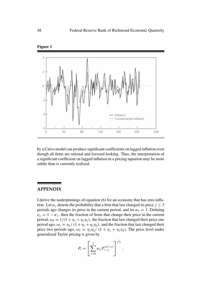
48 Federal Reserve Bank of Richmond Economic Quarterly
Figure 1
by a Calvo model can produce significant coefficients on lagged inflation eventhough all firms are rational and forward looking. Thus, the interpretation ofa significant coefficient on lagged inflation in a pricing equation may be moresubtle than is currently realized.
APPENDIX
I derive the underpinnings of equation (6) for an economy that has zero infla-tion. Let αj denote the probability that a firm that last changed its price j ≤ 3periods ago changes its price in the current period, and let α3 = 1. Definingηj = 1 − αj , then the fraction of firms that change their price in the currentperiod, ω0 = 1/(1 + η1 + η1η2), the fraction that last changed their price oneperiod ago, ω1 = η1/ (1 + η1 + η1η2), and the fraction that last changed theirprice two periods ago, ω2 = η1η2/ (1 + η1 + η1η2). The price level undergeneralized Taylor pricing is given by
Pt = 2∑j=0
ωjP∗(1−ε)t−j
11−ε
,
M. Dotsey: Interpreting Tests of Backward-Looking Pricing 49
where variables are in levels and ε is the elasticity of demand for the firm’sproduct. The optimal price-setting equation is
p∗t = ε
ε − 1
∑2j=0 β
jEt{(ωj/ω0) · (λt+j /λt ) · ψt+j · (Pt+j /Pt)ε · yt+j }∑2j=0 β
jEt{(ωj/ω0) · (λt+j /λt ) · (Pt+j /Pt)ε−1 · yt+j },
where y is the firm’s level of output and βjEt(λt+j /λt ) is the rate at whichprofits are discounted. For more detail concerning the derivation of these twoequations, see Dotsey, King, and Wolman (1999).
Log-linearizing the expression for the price level around zero steady stateinflation yields pt = ω0p
∗t + ω1p
∗t−1 + ω2p
∗t−2, which is (4) in the text. Log
linearizing the equation for the optimal price yields
p∗t = ρ0(ψt + pt)+ ρ1Et(ψt+1 + pt+1)+ ρ2Et(ψt+2 + pt+2),
which is (5), where ρ0 = 1/�, ρ1 = βη1/�, and ρ2 = β2η1η2/�, and� = 1 + βη1 + β2η1η2. The linearization turns out to be so compact becauseat zero inflation many of the terms cancel out (for a general derivation, againsee Dotsey, King, and Wolman [1999]).
Combining (4) and (5) for the prices p∗t , p
∗t−1, and p∗
t−2 yields the follow-ing difference equation:
{1 + a1L+ (a2 − 1/(ω0ρ2))L2 + a3L
3 + a4L4}Et−2pt+2 =
{1 + a1L+ a2L2 + a3L
3 + a4L4}Et−2ψt+2,
where a1 = (1 + βη1)/(βη2), a2 = (1 + βη21 + β2η2
1η22)/(β
2η1η2), a3 =(1 + βη1η2)/(β
2η2), and a4 = 1/β2. One of the roots of the polynomial onEt−2pt+2 is one, and factoring this root yields (6),
{1 + c1L+ c2L2 + c3L
3}Et−2πt+2 =−{1 + a1L+ a2L
2 + a3L3 + a4L
4}Et−2ψt+2,
where c1 = 1 + (1 + βη1η2)/(βη2), c2 = −(1 + η2 + βη1η2)/(β2η2), and
c3 = −1/β2.
REFERENCES
Ball, Lawrence J. 1994. “Credible Disinflation with StaggeredPrice-Setting.” American Economic Review 84 (March): 282–89.
Calvo, Guillermo A. 1983. “Staggered Prices in a Utility-MaximizingFramework.” Journal of Monetary Economics 12 (September): 383–98.
Dotsey, Michael, and Robert G. King. 2001. “Pricing Production andPersistence.” NBER Working Paper 8407 (August).

50 Federal Reserve Bank of Richmond Economic Quarterly
, and Alex L. Wolman. 1999. “State Dependent Pricing andthe General Equilibrium Dynamics of Money and Output.” QuarterlyJournal of Economics 114 (May): 655–90.
Fuhrer, Jeffrey C. 1997. “The (Un)Importance of Forward-Looking Behaviorin Price Specifications.” Journal of Money, Credit and Banking 29(August): 338–51.
Gali, Jordi, and Mark Gertler. 1999. “Inflation Dynamics: A StructuralEconometric Analysis.” Journal of Monetary Economics 44 (October):195–221.
Guerrieri, Luca. 2001. “Inflation Dynamics.” Manuscript, Board ofGovernors of the Federal Reserve System.
Kiley, Michael T. 1998. “Partial Adjustment and Staggered Price Setting,”Manuscript, Board of Governors of the Federal Reserve System.
Roberts, John M. 2001. “How Well Does the New Keynesian Sticky-PriceModel Fit the Data?” Manuscript, Board of Governors of the FederalReserve System.
Rotemberg, Julio J. 1982. “Sticky Prices in the United States.” Journal ofPolitical Economy 60 (December): 1187–281.
Rudd, Jeremy, and Karl Whalen. 2001. “New Tests of the New-KeynesianPhillips Curve.” Manuscript, Board of Governors of the Federal ReserveSystem.
Sbordone, Argia M. 1998. “Prices and Unit Labor Costs: A New Test ofPrice Stickiness.” Manuscript, Rutgers University.
. 2001. “An Optimizing Model of U.S. Wage and PriceDynamics.” Manuscript, Rutgers University.
Taylor, John B. 1980. “Aggregate Dynamics and Staggered Contracts.”Journal of Political Economy 88 (February): 1–24.
Wolman, Alexander M. 1999. “Sticky Prices, Marginal Cost, and theBehavior of Inflation.” Federal Reserve Bank of Richmond EconomicQuarterly 85 (Fall): 29–48.
Imperfect Competition andthe Pricing of InterbankPayment Services
John A. Weinberg
I n a modern economy, a large fraction of payments for goods and servicesinvolve the services of one or more banks. The provision of paymentservices is, in fact, one of the distinguishing characteristics of banks. A
bank-intermediated payment instrument, such as a check, typically commu-nicates instructions to the buyer’s bank to make payment to the seller or theseller’s bank. Often, then, we think of payment services as being bundledwith the deposit services provided by banks, although this is not always thecase. Credit cards, for instance, involve payments by the card-issuing bank,at which the cardholder need not hold deposits. Still, many payment servicesdo arise naturally as byproducts of holding deposits with a bank, and someauthors have recently begun to focus on this payments function in the theoryof banking (McAndrews and Roberds 1999; Prescott and Weinberg 2000).Checks and debit cards are prominent examples of such payment services, butATM service, which gives people remote access to cash from their depositaccounts, is also an example even though ATM transactions facilitate pur-chases with cash, not bank liabilities. Accordingly, the industrial organizationof the payment services industry, and even the characteristics of the paymentservices provided, will generally depend on the organization of the bankingindustry itself.
One area in which the structure of the banking industry matters for thenature of payment services is that of interbank payments—payments in which
This article derives from work completed while I was a visiting scholar at the Bank ofJapan’s Institute for Monetary and Economic Studies. I thank the Institute staff for theirhospitality and assistance and for their willingness to discuss these issues with me. I alsothank Mike Dotsey, Huberto Ennis, Ned Prescott, and Tom Humphrey for helpful comments.The views expressed herein are the author’s and do not necessarily represent the views of theFederal Reserve Bank of Richmond or the Federal Reserve System.
Federal Reserve Bank of Richmond Economic Quarterly Volume 88/1 Winter 2002 51

52 Federal Reserve Bank of Richmond Economic Quarterly
the services of more than one bank are required. In an economy where bankingis dominated by a very few institutions, there may be a relatively large numberof transactions in which the buyer and the seller have deposits with the samebank. In these cases, interbank payments are not necessary. On the otherhand, if there are many banks and people frequently engage in transactionswith customers of diverse institutions, then many payments will be interbankpayments, requiring the services of both the buyer’s and the seller’s banks. Inthese cases each bank provides services to both its own and the other bank’sdepositors. The interbank payment services that one bank provides to another’sdepositors resemble the interconnection services that allow customers of onecommunication network to connect with those of a second network.1
In an environment in which banks compete for depositors, the terms onwhich they make interbank services available can be powerful strategic tools.By making interconnection very costly, a bank could dissuade potential de-positors from placing deposits with competing banks. Such surcharges forinterbank services create inefficiency by exceeding the resource costs of pro-viding those services. Hence, there is potential tension between a bank’s needto compete for depositors and its need to cooperate in interconnection in orderto enhance the quality of its service. The implications of this tension dependon the market structure and the nature of competition in the banking industry.In a perfectly competitive, or perfectly “contestable” market, there is strongreason to expect efficient outcomes, even taking the network characteristicsof payment services into account (Weinberg 1997). Competition, however,may be limited by regulatory or other features of the economic environment.For instance, in the United States, banking was historically segmented alonggeographic lines by an array of branching restrictions. In Japan, such segmen-tation was perhaps even more extensive, with different classes of institutionshaving specified sets of services or classes of customers they could serve (Ito1992). In both of these countries, old barriers between market segments haveeroded, increasing the opportunities for direct competition among a widerarray of banks. Still, in many economies, limits to competition may remain.
In a segmented environment, the terms of interbank payment arrange-ments can have at most a limited effect on the competition among banks fordepositors. The main concern in such an environment, then, would be theprovision of the common resource represented by a comprehensive interbanknetwork. Any conflicts of interest among banks would be mainly related todifferences in the value that different banks placed on having access to such anetwork. For instance, in a banking system in which local clearing houses playan important role in payments within a region, a primary role of an interre-gional network is to connect the various clearing houses. Accordingly, banksthat serve limited geographic areas will be most interested in the services of an
1 Laffont and Tirole (1998a,b) study interconnection pricing among rival telecommunicationnetworks. McAndrews (1998) applies their model to an interbank setting.

J. A. Weinberg: Pricing of Interbank Payment Services 53
interregional interbank network. In Japan, where there have traditionally beenboth regional and nationwide banks, the value of participating in an interbank,interregional network is likely smaller for the latter than for the former. Alarge, nationwide bank could use its own internal branch network to makeconnections among the various clearing houses. A bank with geographicallylimited operations, however, could benefit from having access to a nationalnetwork. Indeed, in the 1940s, when the national clearing system was firstestablished, regional banks took the greatest interest in its development, ac-cording to Tsurumi (1999). By way of contrast, the United States had nonationwide banks at the time of the founding of the Federal Reserve System,and the banks that lobbied for the Fed to create a national network for clearinginterregional checks were primarily large banks in large cities (Lacker, Walker,and Weinberg 1999).
The pricing of interbank payment services typically falls into one of twobroad categories: cooperative or independent. Independent pricing simplymeans that each bank sets the price for its own interbank services. Fees forclearing and settling checks were set independently in the period prior to theFed’s dominance of the check-clearing system. A contemporary example isthe surcharge imposed by a bank for an ATM withdrawal by another bank’sdepositor. Cooperative price-setting usually takes the form of interbank pricesset by a group or consortium of banks. Interchange fees in a payment card orATM network are examples of this sort of cooperation.
It is generally accepted that cooperation among competing firms in thesetting of prices can enable sellers to achieve higher prices and profits thanthey could obtain with independent pricing. This increase in profits comes atthe expense of consumer welfare and economic efficiency. This principle is,of course, the basis for antitrust policy. On the other hand, when firms withsome market power sell complementary goods, then cooperation can resultin lower prices. When it bundles deposit and payment services, a bank isselling products that are both substitutes for and complements to the productsof its rivals. This combination complicates the evaluation of cooperative price-setting.
This article explores the differences between cooperative and independentsetting of interbank prices in alternative market environments. I focus specif-ically on the pricing of interbank payment services when deposit markets aresegmented, as compared to when banks compete directly for deposits. Animportant qualification of this discussion is that it takes the structure of thebanking market, given by the set of potential market participants, as fixed.That is, I do not consider the effects of free entry or potential competition.In essence, then, the article explores how changes in the degree of imperfectcompetition affect the comparison of cooperative and independent pricing.
I address the question of how interbank pricing might respond to a changein the competitive environment in which banks operate, first in fairly general

54 Federal Reserve Bank of Richmond Economic Quarterly
terms and then in the context of a simple model of bank competition and inter-connection. The main insight drawn from this discussion can be summarizedas follows. Cooperation in the setting of interbank prices typically leads tolower interbank prices and greater consumer welfare and profits when depositmarkets are segmented. On the other hand, when banks compete directly fordeposits, cooperation in setting interbank prices can have the effect of damp-ening competition in the deposit market, given a fixed set of competitors. Thiscould result in higher interbank prices and reduced consumer welfare.
1. THE ELEMENTS OF AN INTERBANK PRICING GAME
I begin by describing a model of price competition between two banks facingdemands for deposits and interbank payment services. The demand structurespecified below can be derived from a more detailed economic environmentinvolving the need for agents to engage sometimes in storage and consumptionactivities at physically distinct locations.2 The same general structure wouldarise in any economic environment in which a diverse set of buyers and sell-ers of goods and services acquire both deposit and transaction services frompotentially competing banks. While models adapted from the telecommuni-cations literature can fit into this framework, the general structure allows forsome additional important features. Specifically, and as will be shown by theexample in Section 2, this framework can accommodate differences betweencompeting banks. This is a useful feature since many discussions of compe-tition among banks focus on the relative competitive positions of large andsmall banks.
Demand Functions and Prices
Consider a market in which two banks raise deposits that can be used to makepayments in the purchase of goods. To be concrete, focus on the market forhousehold deposits and the payment services provided by banks to house-holds for making purchases from firms. Also, in the interest of simplicity,suppose that firms are exogenously assigned to banks, some with each bank.A consumer selects a bank at which to deposit; the consumer’s choice willaffect the set of firms to which it can costlessly make payments. If we assumethat consumers are randomly matched with firms for the purpose of makingpurchases, then each consumer faces some chance that he or she will need tomake a purchase from a firm that does not use his or her bank. Completionof such a transaction will require an interbank transaction, in which the firm’sbank credits the firm’s account and collects funds from the consumer’s bank.
2 See Weinberg (2000).

J. A. Weinberg: Pricing of Interbank Payment Services 55
In order to examine interbank pricing and competition, the descriptionof this market structure must specify demand functions for bank services.Labeling the banks 0 and 1, let zi represent the number of depositors attractedby bank i, and let xi represent the number of interbank transactions enteredinto by a customer of bank i.3 These quantities will respond to the prices setby the two banks. Assume that each bank sets two prices, one price for depositservices that also covers all same-bank payments and another price for eachinterbank transaction. Let bank i’s price for deposit services be denoted by piand let its price for an interbank transaction be given by qi . More precisely,bank i collects pi from each consumer who places deposits with it and collectsqi from the other bank’s depositors for each purchase they make from firmsthat use bank i.A more general pricing structure would allow a bank to chargetransaction fees to its own depositors as well as to its rival’s depositors. Thesimpler structure specified here is sufficient to capture the combination ofcomplementarity and substitutability that banks face when they make pricingdecisions.4
The actions of the banks and their customers proceed through three stages.First, banks announce their prices. Next, depositors choose with which bank toplace their funds. Finally, depositors make purchases. If a depositor wishes tomake a purchase from a seller that is associated with a different bank, then thedepositor needs the services of the seller’s bank to complete the purchase. Thedepositor values both the consumption of goods purchased and the depositsleft over after buying goods and paying bank fees.
In general, one can assume that both the number of depositors a bankattracts and the number of interbank transactions it services will be functionsof the full set of prices, (p0, p1, q0, q1). In choosing a bank, a depositor willweigh the value of depositing at bank 0 against the value of depositing at bank1 and against the value of not using banking services at all. The value to adepositor of placing deposits with bank i depends on (pi, qj ). The demandfor deposits at bank 1 (z1) is decreasing in p1 and q0 and either independentof or increasing in p0 and q1.5 An increase in q0 causes this demand to fallbecause q0 is the price paid by bank 1’s depositors when they must make apurchase from a customer of bank 0. The dependence of z1 on p0 and q1 isdetermined by the degree to which the two banks’ markets for deposits aresegmented. Segmentation of the markets could be the result of fundamentaldemand characteristics, such as the degree to which consumers find the depositservices of the two banks to be good substitutes. Market segmentation could
3 This specification treats zi as both the number of depositors and the value of depositsattracted. Hence, each consumer is assumed to have one unit of funds available for deposit.
4 The interaction between interbank pricing and the pricing of services to one’s own depositorsunder more general pricing structures is qualitatively similar to that presented in this article.
5 The treatment of the demand facing bank 0 is symmetric to that for bank 1.

56 Federal Reserve Bank of Richmond Economic Quarterly
also arise from artificial barriers to competition, such as legal rules that limitthe set of consumers a particular bank (or type of bank) may serve.
If there are no consumers who could reasonably choose to bank at eitherbank, then the markets are fully segmented and p0 and q1 will have no effecton z1. If, on the other hand, the two banks compete directly for at least somecustomers, then z1 is increasing in p0 and q1, which determine the cost ofdepositing with bank 0.
For a given depositor at bank 1, the demand for interbank transactionsdepends only on q0, the price charged for such transactions. This is due tothe assumed timing of the depositor’s decisions. When the depositor makes aconsumption decision (chooses x), deposits have already been placed with abank. Hence, the depositor’s only remaining decision is to weigh the marginalutility of consumption against its price. Here, the price of consumption is eitherzero (if the depositor is buying from a seller who uses the same bank as thedepositor) or qj for an interbank purchase (from a seller that uses the other bank[bank j ]). The total quantity of interbank transactions on which bank 0 collectsq0 is z1x1. The banks’ profits can be written as�1 = z1p1 + z0x0(q1 − c) and�0 = z0p0 + z1x1(q0 − c), where c is the cost to the bank of processing andcollecting on an interbank payment.6
Pricing Behavior
The banks set prices for payment and deposit services to maximize their profits,each taking the other’s prices as given. Consider, for instance, bank 1’s profitmaximization problem. Its first order conditions are7
∂�1
∂p1= z1 + ∂z1
∂p1p1 + ∂z0
∂p1x0(q1 − c) = 0; and
∂�1
∂q1= z0x0 + ∂z1
∂q1p1 + (
∂z0
∂q1x0 + ∂x0
∂q1z0)(q1 − c) = 0.
These two equations can be rewritten as
1 + η1p1
+ η0p1
z0x0(q1 − c)
p1z1= 0; and
1 + µ1(η0q1
+ ε0q1)+ η1
q1
z1p1
z0x0q1= 0,
where ηij is the elasticity of zi (demand for deposits at bank i) with respect toprice j ; εij is the elasticity xi (demand for interbank payment services from
6 The profit functions reflect the assumption (for simplicity) that variable costs of depositservices are zero.
7 Similar conditions hold for bank 0.
J. A. Weinberg: Pricing of Interbank Payment Services 57
bank i) with respect to price j ; and µi = qi−cqi
is the percent mark-up of bank
i’s interbank price over marginal cost.8
The conditions above capture the typical result that a profit-maximizingprice is inversely related to the relevant (own-price) demand elasticities. Thefirst condition indicates that, in addition to the price elasticity of its own depositdemand, a bank’s choice of a price for its deposit services also depends on thecross-price elasticity of the other bank’s deposit demand. This dependencearises because the bank earns profits by providing interbank payment servicesto its rival’s depositors. Since deposits at the two banks are substitute services,own-price and cross-price elasticities have opposite signs; raising bank 1’sown deposit price increases bank 0’s deposits, thereby increasing bank 1’sinterbank services. The effect is to amplify a bank’s desire to raise depositprices, other things being equal. The magnitude of this effect depends on therelative contributions that payment services and deposit services make to abank’s profits.
A similar interpretation can be given to the second condition above. Whensetting its price on payment services, a bank considers both the direct effect ofthe price on its own sale of payment services and the indirect effect on its saleof deposit services. The latter results because bank 1’s payment services arecomplementary to bank 0’s deposit services, which are substitutes for bank1’s own deposit services. Again, the strength of the indirect effect depends onthe relative contributions the two services make to a bank’s overall business.
Segmented Markets
The joint solution of the two banks’ problems and the nature of the interactionbetween prices of interbank payment services and prices of basic depositservices depend on the nature of competition between the banks. In part,the nature of interbank rivalry is determined by the structure of the banks’external environment. In particular, the degree of integration or segmentationof markets determines whether the banks come into face-to-face competitionwith each other. This characteristic of the markets is captured by the demandfunctions, and the degree of segmentation is represented by the values of theelasticities ηipj , for i �= j , and ηiqi . These elasticities reflect the responsivenessof a bank’s deposits to the other bank’s deposit price and to its own interbankpayment price. Recall that a bank’s interbank price is paid by the other bank’sdepositors. Hence, q1 will affect z1 only if banks 1 and 0 compete directlyfor customers. When the deposit markets are segmented, η0
p1= η1
p0= η0
q0=
η1q1
= 0.
8 It is common to express own-price elasticities as absolute values. Here, ηipi and εiqiare
defined as negative numbers. This seems convenient, as own-price elasticities are combined insome expressions with cross-price elasticities, which may be negative or positive.
58 Federal Reserve Bank of Richmond Economic Quarterly
When markets are segmented, then the first order conditions above reduceto
∂�1
∂p1= z1 + ∂z1
∂p1p1 = 0; and
∂�1
∂q1= z0x0 + (
∂z0
∂q1x0 + ∂x0
∂q1z0)(q1 − c) = 0.
Or, in terms of elasticities,
1 + η1p1
= 0; and
1 + µ1(η0q1
+ ε0q1) = 0.
Note that even when markets are segmented, one bank’s pricing is notentirely independent of the other bank’s prices. Each bank’s deposit demanddepends on its own deposit price and the other bank’s payment service (inter-connection) price. That is, z1 depends on p1 and q0. Still, under segmentedmarkets, a bank’s pricing of its own deposit services does not interact directlywith its pricing of interbank payment services.
In the case of segmented markets, one bank’s deposit services are com-plementary to the other bank’s interbank payment services. For instance, anincrease in q0, bank 0’s payment service price, reduces the value to potentialcustomers of placing deposits at bank 1. The price increase will generallyresult in lower demand for bank 1 deposits and lower profit-maximizing valueof p1, bank 1’s deposit price. At the same time, an increase in p0 reduces thetotal value of deposits bank 0 is able to attract and correspondingly reducesthe volume of interbank transactions on which bank 1 can extract a fee. Thisreduction in demand results in a lower optimal choice of q1.
When two sellers set the prices of complementary goods noncooperatively,the outcome is often characterized as a problem of “double-marginalization.”In effect, the two goods can be thought of as a single service with two distinctcomponents. If both components were sold by a single seller with marketpower, that seller would recognize the effect of each component’s price on thesale of both components. This interdependence limits the seller’s interest inraising prices. When the components are sold separately by different firms,each seller is interested in only its own profits and ignores the effects of its priceon the other seller’s sales. As a result, the distortion due to the deviation ofprice from marginal cost is compounded by the independent profit-maximizingbehavior of two sellers with market power. This compound distortion comesat the cost of both combined seller profits and consumer welfare. Hence, theindependent pricing of complementary goods resembles decisionmaking insettings with externalities. Each bank ignores the effect of its interbank priceon the sales of the other bank, and their noncooperation leads to a loss ofefficiency. Unlike losses occurring in the case of a true externality, however,

J. A. Weinberg: Pricing of Interbank Payment Services 59
this loss occurs here only because competition is imperfect and each bankexercises some market power. If for instance there were additional bankswhose deposit and payment services were perfect substitutes for those of bank0, then both p0 and q0 would be competed down to marginal cost. The samewould be true for bank 1 in the presence of additional competition.
If instead of setting all prices noncooperatively, banks set their prices forinterbank services through negotiation, they can raise their combined profitsby setting interbank prices (q0 and q1) lower than their noncooperative levels.This process is formalized by assuming that q0 and q1 are set to maximizejoint profits, conditional on the noncooperative determination of p0 and p1.The process represents a mixed form of interaction between sellers in whichthey collude on interbank prices while they compete in the pricing of depositservices. For many specifications of the demand structure, the optimal nego-tiated choice for interbank prices is to set them equal to marginal cost. Thischoice eliminates the double marginalization problem, allowing banks to earntheir rents from the markup on deposit services. When deposit markets aresegmented, cooperation in setting the interbank prices is equivalent to full co-operation in setting all prices, for banks are local monopolists in their depositmarket segments.
To see the effects of cooperating in interbank price-setting in segmentedmarkets, consider the first order condition for choosing q1 to maximize jointprofits (�0 +�1). In terms of elasticities,
1 + η0q1
p0
(q1 − c)x0+ µ1(η
0q1
+ ε0q1) = 0.
This cooperative condition has one more term than the correspondingnoncooperative condition: η0
q1
p0(q1−c)x0
. The extra term reflects the effect ofbank 1’s choice of interbank price q1 on bank 0’s earnings from depositspriced at p0. The effect of the added term is to reduce the choice of q1, otherthings being equal.
In segmented markets, the mechanism for jointly determining interbankprices is not a matter of great importance. Suppose the jointly optimal inter-bank prices are q0 = q1 = q. A relatively simple mechanism that will achievethis result is to delegate the choice of a common interbank price to one of thebanks. That is, impose symmetry in interbank prices and let the price level bechosen by either of the banks. Suppose this authority is granted to bank 0. Itschoice of q0 does not affect its own profits, but q1 does. If the demands facingthe two banks are symmetric, then bank 0’s optimal choice is to set q0 = q.Bank 1 would make the same choice if it were given the authority to set the q’s.Hence, with segmented markets and symmetric demands, delegated setting ofreciprocal interbank prices achieves the same interbank price as would be setunder joint profit maximization, subject to noncooperative choices of depositprices. This mechanism, then, results in lower interbank prices than would be
60 Federal Reserve Bank of Richmond Economic Quarterly
chosen independently by the two banks. There are some cases in which thismechanism results in interbank prices that are equal to marginal cost.
When markets are not segmented, the interaction between deposit pricesand payment service prices is more complicated. In this case, the interbankprices (q0, q1) are a strategic tool in competition for market share. In additionto raising revenue for bank 0, q0 imposes a cost on bank 1’s depositors that,other things being equal, may induce some consumers to deposit at bank 0instead. To the extent that bank 0 is able to extract price-cost margins fromdeposit customers that are large relative to markups on payment services, thebank may find it profitable to use a high interbank price to help attract de-posits. It is also not the case that cooperation in setting interbank prices willnecessarily improve consumer welfare. That cooperation has ambiguous con-sequences is one of the messages of the literature on interconnection pricing intelecommunications networks. The interbank price could facilitate collusionin deposit pricing by making depositors less likely to switch banks.
It may be reasonable to think of an increase in competition (or more pre-cisely in the potential competitiveness of the market environment) as beingcaptured by a move from segmented markets to a single integrated market.Such a shift could have many causes. Changes in the regulatory or legalenvironment could bring banks that had previously enjoyed protected mar-ket segments into direct competition. Improvements in technology can makeit possible for banks to serve expanding sets of customers. For instance,consumer banking may traditionally have been a local business, with peoplechoosing banks based on their proximity to home or place of business. Tech-nological advances allow consumers to make banking choices that are lessdependent on location.
If we think of increasing competition as a shift from segmented to in-tegrated markets, then it becomes clear that the role of interbank prices canchange in a more competitive environment. With less competition (segmentedmarkets) the interbank price serves mainly as a potential source for doublemarginalization. Accordingly, cooperation in setting the interbank price islargely beneficial from the point of view of consumer welfare. As marketsbecome more competitive (integrated), the interbank price plays a more com-plicated strategic role.
Of course, the degree of competition between two banks also depends inpart on the behavior of the banks themselves. Is their pricing competitive, inthe sense that price determination can be modeled as the Nash equilibrium ofa noncooperative game? Or is there some amount of cooperation between thebanks in their price-setting behavior? This aspect of the degree of competitionis more difficult to tie directly to the demand and cost fundamentals of themarket. Rather, the ability of banks to collude depends on such factors asthe legal environment. In a setting with strict antitrust enforcement, it will bedifficult for sellers of a product or service to engage in explicit or open price

J. A. Weinberg: Pricing of Interbank Payment Services 61
collusion. Even so, tacit collusion may be possible, in the form of cooperationsupported by implicit threats to engage in a price war should any seller cheaton the collusive agreement.9 The feasibility of such collusion depends onfactors like sellers’ ability to monitor each other’s behavior.
The foregoing discussion has assumed that banks behave as Nash price-setters. Under that assumption, the degree of competition is determined bythe demand characteristics, as discussed above.
Suppose that banks do collude in the setting of all prices. In that case,prices are set to maximize joint profits, �0 +�1. In this case, the first orderconditions for (for instance) (p1, q1) are
∂(�0 +�1)
∂p1= z1 + ∂z1
∂p1[p1 + x1(q0 − c)] + ∂z0
∂p1[p0 + x0(q1 − c)] = 0;
and
∂(�0 +�1)
∂q1= ∂z1
∂q1[p1 + x1(q0 − c)] + ∂z0
∂q1[p0 + x0(q1 − c)]
+z0[∂x0
∂q1(q1 − c)+ x0]
= 0.
As with other conditions stated above, these last two can be expressed interms of demand elasticities as
1 + η1p1
[1 + x1(q0 − c)
p1] + η0
p1
p0z0 + z0x0(q1 − c)
p1z1= 0; and
1 + µ1(η0q1
+ ε0q1)+ η0
q1
p0
x0q1+ η1
q1
z1p1 + z1x1(q0 − c)
z0x0q1= 0.
For any given configuration of demand, cooperative price-setting tends toresult in higher deposit prices (p’s) and lower payment services prices (q’s)than does noncooperative pricing. Payment services provide interconnectionbetween banks, allowing one bank’s customers to use another bank’s facilities.The prices charged for these services, then, are prices charged to anotherbank’s depositors. When prices are set noncooperatively, a bank ignores theeffect that raising the payment services price has on its rival’s demand andprofits. Taking this effect into account initiates cooperation, which results ina moderation of the desire to raise this price. Hence, when banks colludein the setting of deposit prices, either explicitly or implicitly, the role of theinterbank price resembles its role in segmented markets.
9 Green and Porter (1984).

62 Federal Reserve Bank of Richmond Economic Quarterly
One additional issue regarding tacit (or implicit) collusion involves therole that interbank prices might play in coordinating collusive pricing. Banksmust monitor implicit agreements not to engage in aggressive competition indeposit prices, and the monitoring of a rival bank’s deposit arrangements withits customers may be difficult compared to monitoring prices of interbankpayment services. If, for instance, bank 1 charges a fee to bank 0’s depositor,that fee is typically collected through bank 0 (that is, through the interbankclearing and settlement system). Hence, bank 0 will directly observe thefees its customers face from bank 1. The ease of monitoring interbank pricescould give them a role to play in the enforcement of broader agreements amongbanks.
2. AN EXAMPLE
The strategic interaction among banks (or firms in general ) in setting inter-connection prices can be illustrated by an example in which consumers areassumed to have “home” locations on the “Hotelling” line (Hotelling 1929).That is, each consumer’s location is given by a point in the unit interval,z ∈ [0, 1]. There are two banks, located at either end point of the interval.The cost to a consumer located at z of depositing funds at bank 0 is τz, and thecost of depositing at bank 1 is τ(1 − z). A consumer receives utility W fromdeposit services and U from payment services. One could interpret W as thebalances deposited with the bank. If the consumer is able to use his or herdeposit balances to make a purchase of goods from a store, then U will repre-sent the net benefit that the consumer receives from such a transaction. Hence,a “payment service” here might be a transfer of funds from the consumer’saccount to the store’s account. Alternatively, a payment service might be thewithdrawal of cash at a cash dispensing terminal close to the place where theconsumer will make a purchase. In either case, the net value received by theconsumer will be W + U minus fees paid to banks. A consumer also hasthe option of not depositing funds in a bank. For simplicity, assume that bynot using bank services the consumer limits his or her ability to make certainpurchases. Specifying the value to the consumer of not depositing funds witha bank as W captures this assumption.
Consumers face uncertainty about where they will want to consume finalgoods. This uncertainty translates into uncertainty regarding the bank fromwhich the consumer will need deposit services. With probabilityφ, a consumerneeds the services of bank 0. This might be interpreted as a consumer’s desireto transfer funds to a merchant who banks with bank 0 or as a consumer’sneed to withdraw funds from a machine owned by bank 0. With probability(1 − φ), the consumer needs the payment services of bank 1.
Bank i bundles deposit services and payment services to its own deposi-tors under a single price pi and charges qi for payment services provided to

J. A. Weinberg: Pricing of Interbank Payment Services 63
the other bank’s depositors. The net benefits that a consumer derives fromdepositing with either bank are given by
V0 = W + U − p0 − (1 − φ)q1 − τz; and
V1 = W + U − p1 − φq0 − τ(1 − z).
If, for a given z, the greater of V0 and V1 is greater than W , then theconsumer deposits with whichever offers the greater value. Let zi denotethe consumer for whom Vi = W . Then, the case of segmented markets, asdiscussed above, is the case in which z0 < z1. In this case, there is a setof consumers (those between z0 and z1) who do not use banking services.Consumers between 0 and z0 deposit at bank 0, while those between z1 and 1deposit at bank 1. Given this specification of demand, banks’ profit functions(when markets are segmented) can be written as10
�0 = z0p0 + φ(1 − z1)q0; and
�1 = (1 − z1)p1 + (1 − φ)z0q1.
This specification of segmented markets involves a “gap” in the marketfor banking services that represents consumers who choose not to deposittheir funds in the banking system. While there are, in fact, such “unbanked”consumers in many economies (close to 10 percent of all households in theUnited States), one need not take this specification literally. The choice ofinterbank prices would be similar in any setting in which a bank’s choice of qhad no effect on its own deposits. This would be true, for instance, if depositmarket segmentation were established by legal or regulatory rules.
Noncooperative price-setting by banks in this example leads to the fol-lowing Nash equilibrium prices: p0 = p1 = U
3 ; q0 = min[ U3φ , U ]; q1 =min[ U
3(1−φ) , U ]. The reason interbank prices must be less than U is that con-sumers can always choose not to use interbank services, forgoing the utilityU.With these prices, the market division is given by z0 = (1 − z1) = U
3τ , sothat the two banks have equal market shares.11
When the noncooperative equilibrium has this segmented markets char-acteristic, cooperation in the setting of interconnection prices is equivalent tofull cooperation in all prices. This is true because with segmented markets,each bank is a local monopolist in its segment of the deposit services market.Still, cooperation results in a preferred outcome for both banks and consumers.
10 For simplicity, this example assumes that the marginal costs of both deposit and paymentservices are zero. Assuming positive marginal costs would not alter the nature of the strategicinteraction among banks. However, assuming a higher marginal cost for interbank payment servicesthan for same bank services would add an important dimension to the efficiency properties ofequilibrium allocations.
11 This characterization of the equilibrium assumes that τ > 23U .

64 Federal Reserve Bank of Richmond Economic Quarterly
Under this pricing scenario, interbank prices (q0, q1) are set equal to marginalcost (q0 = q1 = 0), and deposit prices are p0 = p1 = U
2 . Hence, depositprices go up while interbank charges go down. The net effect on consumerwelfare is positive, as is demonstrated by the fact that more consumers chooseto use bank services under this pricing scenario than under noncooperativepricing. With the cooperative prices, market shares are z0 = z1 = U
2τ .Whether the equilibrium features segmented or integrated markets de-
pends, of course, on the parameters of the model. In particular, U givesthe value of having access to payment services, and τ gives the consumer’smarginal cost of using bank services. As τ gets smaller or U gets bigger,more consumers will seek to use bank services, and eventually the marginalconsumer’s decision will be between banks rather than whether to deposit atall. When the market becomes integrated in this way, banks’ shares of themarket are determined by the point (z), at which a consumer is indifferentbetween the two banks (V0 = V1 > W ). Denoting this point by z, we have
z = 1
2+ 1
τ[(p1 + φq0)− (p0 + (1 − φ)q1)],
and banks’ profit functions are
�0 = zp0 + φ(1 − z)q0,
�1 = (1 − z)p1 + (1 − φ)zq0.
Under these conditions, banks have a heightened incentive to raise theinterconnection price compared to the case of segmented markets. With seg-mented markets, q0 has no effect on bank 0’s sale of deposit services to itsown customers. Here, raising q0 raises the cost to consumers of depositingwith bank 1. When the market is integrated, any loss of depositors by bank 1is matched by a gain at bank 0. Indeed, in this example the profit-maximizingchoice for q0 and q1 is q0 = q1 = U . Deposit prices are then p0 = 2τ + φU
and p0 = 2τ + (1 − φ)U .With an integrated market, it is no longer true that banks can raise their
combined profits by agreeing to lower interconnection prices. In particular,each bank’s profits are lower if interconnection prices are set at marginalcost. That is, cooperation on interbank prices alone does not tend to drivethose prices down to marginal cost. On the other hand, if banks collude onboth interbank and deposit prices, then joint profits are maximized by settinginterbank prices equal to zero.12
12 Actually, in this example, where consumers end up using either zero or one unit of inter-bank services, the joint profit maximizing solution determines only the sums p0 + (1 − φ)q1 andp1 + φq0. In an extended example, with downward sloping demand for interbank services, jointmaximization would drive the interbank prices to marginal cost.

J. A. Weinberg: Pricing of Interbank Payment Services 65
3. CONCLUSION
In many economies, the business of banking is undergoing profound changes.Boundaries between markets, both geographically and in terms of productlines, are being removed by regulatory changes and technological advances.These changes present challenges to traditional ways of handling interbankclearing and settlement arrangements. If the terms for interbank transactionsare established by industry-based, collaborative organizations, how will sucharrangements respond to the entry of new market participants? This articlehas suggested that increasing (though still imperfect) competition creates acomplicated set of incentives for banks with regard to the terms for inter-bank payment services. Neither competition nor cooperation in setting theseprices is guaranteed to always yield desirable results from the point of viewof consumer welfare. This does not necessarily imply the need for a regula-tory mechanism in determining interbank prices. The development of sucha mechanism, managed by a governmental authority, is subject to its owndrawbacks—including, for instance, the difficulty faced by a regulator in ob-taining the information necessary to set optimal interconnection prices. Ratherthan direct regulation, however, there may be call to carefully monitor of in-dustry practices in interconnection pricing. Such monitoring was perhaps lessimportant in an environment with less direct competition among banks. Itis somewhat ironic, then, that increasing competition may actually increaseconcerns for the competitive impact of interbank payment services pricing.
REFERENCES
Green, Edward J., and Robert H. Porter. 1984. “Noncooperative Collusionunder Imperfect Price Information.” Econometrica 52: 87–100.
Hotelling, Harold. 1929. “Stability in Competition.” The Economic Journal39 (March): 41–57.
Ito, Takatoshi. 1992. The Japanese Economy. Cambridge, Mass.: The MITPress.
Lacker, Jeffrey M., Jeffrey Walker, and John A. Weinberg. 1999. “The Fed’sEntry into Check Clearing Reconsidered.” Federal Reserve Bank ofRichmond Economic Quarterly 85 (Spring): 1–31.
Laffont, Jean J., Patrick Rey, and Jean Tirole. 1998a. “Network CompetitionI: Overview and Nondiscriminatory Pricing.” Rand Journal ofEconomics 29 (Spring): 1–37.
66 Federal Reserve Bank of Richmond Economic Quarterly
. 1998b. “Network Competition II: Price Discrimination.”Rand Journal of Economics 29 (Spring): 38-56.
McAndrews, James. 1998. “Direct Presentment Regulation in Payments.”Federal Reserve Bank of Chicago Conference on Bank Structure andPerformance, Proceedings.
, and William Roberds. 1999. “Payment Intermediation andthe Origins of Banking.” Federal Reserve Bank of Atlanta WorkingPaper 99-11.
Prescott, Edward S., and John A. Weinberg. 2000. “Incentives,Communication and Payment Instruments.” Federal Reserve Bank ofRichmond Working Paper 00-11.
Sidak, J. Gregory, and Daniel F. Spulber. 1997. Deregulatory Takings andthe Regulatory Contract. Cambridge: Cambridge University Press.
Tsurumi, Masayoshi. 1999. “The History of the Payment System in Japan.”Manuscript, Faculty of Economics, Hosei University, Tokyo, Japan.
Weinberg, John A. 1997. “The Organization of Private Payment Networks.”Federal Reserve Bank of Richmond Economic Quarterly 82 (Spring):25-43.
. 2000. “Interconnection and Rivalry Between Banks.”Wharton Financial Institutions Center Working Paper 00-15.
Recent Developments inMonetary Policy Analysis:The Roles of Theory andEvidence
Bennett T. McCallum
1. INTRODUCTION
Academic thinking about monetary economics—as well as macroeconomicsmore generally—has altered drastically since 1971–1973 and so has the prac-tice of monetary policy. The former has passed through the rational expecta-tions and real-business-cycle revolutions into today’s “new neoclassical syn-thesis” whereas policymaking has rebounded, after a bad decade followingthe breakdown of the Bretton Woods system, into an era of low inflationthat emphasizes the concepts of central bank independence, transparency, andaccountability while exhibiting substantial interest in the consideration of al-ternative rules for the conduct of monetary policy.1
My assignment in this paper is to consider the roles of economic theory andempirical evidence in bringing about these changes—in particular, changes inpolicy formulation. Have they been driven primarily by theoretical reasoning
H. J. Heinz Professor of Economics, Carnegie Mellon University, and Visiting Scholar, FederalReserve Bank of Richmond. This article previously appeared in the Journal of EconomicMethodology 6:2, 1999: 171–98 (http://www.tandf.co.uk), and in Macroeconomics and the RealWorld, vol. 1 (Oxford University Press 2000) and is reprinted here with permission. It wasprepared for the conference “Theory and Evidence in Macroeconomics,” held 15–17 October1998, in Bergamo, Italy. For helpful suggestions and criticism, I am indebted to MarvinGoodfriend, Jim Hartley, Bob Hetzel, Bob King, Mary Morgan, Edward Nelson, and HaraldUhlig. The views expressed in this article do not necessarily reflect those of the FederalReserve Bank of Richmond or the Federal Reserve System.
1 A different (but not incompatible) account of post-Bretton Woods developments in mone-tary analysis is provided by Goodfriend and King (1997), who coined the term “new neoclassicalsynthesis.”
Federal Reserve Bank of Richmond Economic Quarterly Volume 88/1 Winter 2002 67

68 Federal Reserve Bank of Richmond Economic Quarterly
or by accumulated evidence? As a related matter, has the evolution reflectedhealth or sickness in the macro-monetary branch of economic science?
In discussing actual monetary policymaking, there is a difficulty stem-ming from the possibility that in practice policy choices are dominated byresponses to current political pressures, with economic reasoning of any formplaying a strictly subordinate role in the thought processes of voting mem-bers of policymaking bodies such as the United States Federal Open MarketCommittee. There is reason to believe, however, that economic analysis hasbeen playing an increasing role in monetary policy considerations and, in anyevent, there would be little for economists to discuss if we were to concludethat actual policy is independent of such analysis. Consequently, most of thediscussion below will take writings of central bank economists, together withofficial publications such as inflation reports, as providing some indication ofactual monetary policy practices.
Also, it should be admitted at the outset that evaluation of the relativecontributions of theory and evidence is extremely difficult. In fact, a properquantitative evaluation is probably impossible, since economic science evolvesby way of a complicated back-and-forth interaction of theoretical and empiri-cal considerations. Moreover, these considerations are often combined in thework of a single analyst; for example, most of the researchers listed below inTable 1 rely on such a combination in their own work. Consequently, someof this back-and-forth takes place within the minds of individual researchersand thus may not show up at all in the exposition of papers written to reportresults. Under such circumstances, it is clear that measurement of the relativecontributions of theory and evidence must be highly problematic, at best. Ac-cordingly, what is presented in this paper might be regarded more as a numberof observations relevant to the issue, rather than as an actual evaluation. Myhope is that these observations will shed some light on the evolution of mon-etary analysis while establishing that both theory and evidence have playedimportant roles.
The outline of the paper is as follows. In Section 2, general analytic trendsin macroeconomics will be briefly outlined as a background. Then Section3 takes up the evolution of monetary policymaking in practice and Section 4does the same for the formal analysis of monetary policy. Section 5 treats aspecial topic and Section 6 concludes.
2. TRENDS IN MACROECONOMICS, 1973–1998
The years 1971–1973 make a good starting point for our discussion becausethey mark sharp breaks in both macroeconomic thinking and in institutionalarrangements relevant to the conduct of monetary policy. In terms of institu-tions, of course I have in mind the breakdown of the Bretton Woods exchange-rate system, which was catalyzed by the United States’s decision of August

B. T. McCallum: Developments in Monetary Policy Analysis 69
1971 not to supply gold to other nations’ central banks at $35 per ounce.This abandonment of the system’s nominal anchor naturally led other nationsto be unwilling to continue to peg their currency values to the (overvalued)U.S. dollar, so the par value exchange-rate agreements disintegrated. Newpar values were painfully established in the December 1971 meeting at theSmithsonian Institution, but after a new crisis in February 1973 the par-valuesystem crumbled in March 1973 and has not been reassembled as of 1998.2
In terms of macroeconomics, the years 1971–1973 featured the publica-tion of six papers that initiated the rational expectations revolution. The mostcelebrated of these, certainly, is Lucas’s (1972a) “Expectations and the Neu-trality of Money,” but his (1972b) and (1973) were also extremely influentialas were Sargent’s (1971) and (1973). Curiously, however, the first publicationto use rational expectations in a macro-monetary analysis was none of thesebut rather Walters (1971), which has apparently had almost no influence.3
At first there was much resistance to the hypothesis of rational expec-tations, partly because in macroeconomics it was initially associated ratherstrongly with the policy-ineffectiveness proposition.4 There were also severalother misconceptions, one of which continues today in the argument that itis implausible that all of an economy’s agents would believe in the particularmodel of the economy being used by the analyst.5 Actually, that is not theassumption required for rational expectations. The latter presumes insteadthat agents form expectations so as to avoid systematic expectational errors inactuality, which implies that they behave as if they knew the structure of theactual economy. Then expectations will agree with the analyst’s model of theeconomy, but the reason is that this model is by construction the analyst’s bestattempt to depict the true structure of the economy (otherwise, he/she woulduse a different model).
Be that as it may, the hypothesis of rational expectations (RE) graduallyswept the field in both macroeconomics and microeconomics, a major reasonbeing that it is almost certainly unwise for policy to be conducted under thepresumption that any particular pattern of expectational errors will prevail inthe future—and ruling out all such patterns implies that expectational errorsare orthogonal to information sets (i.e., implies rational expectations). Duringthe late 1970s there was much interest in alternative specifications of price
2 A very brief analysis of the source of the collapse is given below in Section 3.3 One reason, perhaps, is that Walters used a different term, namely, “consistent expectations.”
His paper’s first footnote states in part: “What I call consistent expectations is formally similar toRichard Muth’s rational expectations.” Actually, of course, Richard F. Muth—at the time a leadingscholar in the field of housing economics—is the brother of John F. Muth.
4 On the latter, see McCallum (1980).5 A variant is the claim that it is implausible that all agents would believe in the same model
of the economy. But, first, this is an objection to macroeconomics, not rational expectations, andsecond, there are some rational expectations models in which agents’ expectations are not all alike.
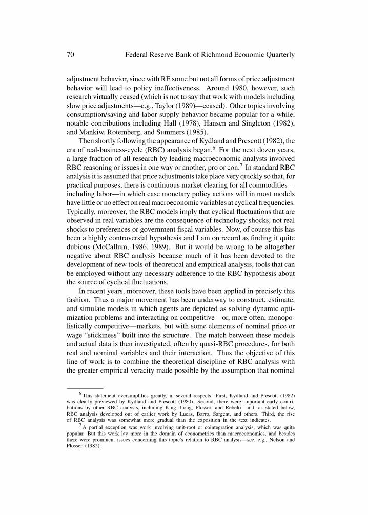
70 Federal Reserve Bank of Richmond Economic Quarterly
adjustment behavior, since with RE some but not all forms of price adjustmentbehavior will lead to policy ineffectiveness. Around 1980, however, suchresearch virtually ceased (which is not to say that work with models includingslow price adjustments—e.g., Taylor (1989)—ceased). Other topics involvingconsumption/saving and labor supply behavior became popular for a while,notable contributions including Hall (1978), Hansen and Singleton (1982),and Mankiw, Rotemberg, and Summers (1985).
Then shortly following the appearance of Kydland and Prescott (1982), theera of real-business-cycle (RBC) analysis began.6 For the next dozen years,a large fraction of all research by leading macroeconomic analysts involvedRBC reasoning or issues in one way or another, pro or con.7 In standard RBCanalysis it is assumed that price adjustments take place very quickly so that, forpractical purposes, there is continuous market clearing for all commodities—including labor—in which case monetary policy actions will in most modelshave little or no effect on real macroeconomic variables at cyclical frequencies.Typically, moreover, the RBC models imply that cyclical fluctuations that areobserved in real variables are the consequence of technology shocks, not realshocks to preferences or government fiscal variables. Now, of course this hasbeen a highly controversial hypothesis and I am on record as finding it quitedubious (McCallum, 1986, 1989). But it would be wrong to be altogethernegative about RBC analysis because much of it has been devoted to thedevelopment of new tools of theoretical and empirical analysis, tools that canbe employed without any necessary adherence to the RBC hypothesis aboutthe source of cyclical fluctuations.
In recent years, moreover, these tools have been applied in precisely thisfashion. Thus a major movement has been underway to construct, estimate,and simulate models in which agents are depicted as solving dynamic opti-mization problems and interacting on competitive—or, more often, monopo-listically competitive—markets, but with some elements of nominal price orwage “stickiness” built into the structure. The match between these modelsand actual data is then investigated, often by quasi-RBC procedures, for bothreal and nominal variables and their interaction. Thus the objective of thisline of work is to combine the theoretical discipline of RBC analysis withthe greater empirical veracity made possible by the assumption that nominal
6 This statement oversimplifies greatly, in several respects. First, Kydland and Prescott (1982)was clearly previewed by Kydland and Prescott (1980). Second, there were important early contri-butions by other RBC analysts, including King, Long, Plosser, and Rebelo—and, as stated below,RBC analysis developed out of earlier work by Lucas, Barro, Sargent, and others. Third, the riseof RBC analysis was somewhat more gradual than the exposition in the text indicates.
7 A partial exception was work involving unit-root or cointegration analysis, which was quitepopular. But this work lay more in the domain of econometrics than macroeconomics, and besidesthere were prominent issues concerning this topic’s relation to RBC analysis—see, e.g., Nelson andPlosser (1982).

B. T. McCallum: Developments in Monetary Policy Analysis 71
prices do not adjust instantaneously.8 Basically, the attempt is to developa model that is truly structural, and therefore immune to the Lucas (1976)critique of econometric policy analysis.
The mere description of these developments in macroeconomics makes itapparent that they have been driven by a combination of theoretical and empir-ical impulses. The rational expectations onslaught was primarily theoreticalin origin, building upon recognition of the fact that all other expectational hy-potheses permit systematic (hence correctable) expectational errors. But thelogical basis for the upsurge of the RBC movement can be viewed as princi-pally empirical.9 Here the point is that RBC models are in essence equilibriumbusiness cycle models of the type promoted by Lucas (1972a, 1975) but withthe monetary shocks eliminated and technology shocks emphasized. And thischange in emphasis came about, it can be argued, largely because empiricalanalysis of various types suggested that the cyclical real effects of monetarypolicy shocks were in fact very small in relation to the overall variability ofoutput and employment. Some crucial studies providing such evidence wereSims (1980), Litterman and Weiss (1989), Eichenbaum and Singleton (1986),and Nelson and Plosser (1982).10
Then there came the more recent movement to incorporate gradual priceadjustment—“sticky prices”— into optimizing macro models. By its verynature, the impetus for this movement must have been mainly empirical. Forthere is no body of theory that tells us that price behavior is sticky; to thecontrary it is rather difficult to incorporate sticky prices in a model that stressesoptimizing general equilibrium theory.11
Thus it has to be the force of evidence that has brought about this importantchange. Moreover, I think it is only fair to recognize that the RBC movementhas itself been strongly concerned with empirical veracity, even though in thatregard its preferred measures have been quite different from those used inorthodox time series econometrics.
8 The first of these papers of which I am aware is King (1990). Other notable efforts withpublication dates prior to 1997 include Benassy (1995), Cho (1993), Cho and Cooley (1995),Cooley and Hansen (1995), Hairault and Portier (1993), Kimball (1995), King and Watson (1996),Rotemberg (1996), Ohanian, Stockman, and Kilian (1995), and Yun (1996). For references and auseful review, see Nelson (1998). Some more recent studies will be mentioned below.
9 This statement has been disputed by several readers, and I must confess that the followingargument is not entirely straightforward. But I continue to believe that the leaders of the RBCmovement were not Keynesians who were won over by arguments for theoretical purity, but insteadwere adherents of the Lucas-Barro equilibrium approach who discovered that it was very difficultempirically to assign much importance to monetary shocks.
10 This is not to imply that these studies are immune to criticism; in fact I have quarreledwith some of them myself. But the point is that, rightly or wrongly, they were influential.
11 One reader has suggested that it is illogical for me to cite “evidence” as providing stimulusfor the rise and also the decline of RBC analysis. But I contend that this is not illogical, fordifferent types of evidence were predominant during the two phases of intellectual development.
72 Federal Reserve Bank of Richmond Economic Quarterly
With respect to these measures a few brief words may be appropriatebefore we move on. The “standard” set of RBC measures was establishedin the famous Kydland-Prescott (1982) paper, which focused on three setsof second moments for variables that had been “detrended.” These were:(i) variances of important real variables including output, labor input, averagelabor productivity, consumption, investment, and capital; (ii) correlations withoutput of the other variables listed in (i); and (iii) autocorrelations and, to alesser extent, lead and lag correlations with output.12 Thus the RBC empiricalverification program has been to assess the conformity of these measures asgenerated by RBC models with actual values pertaining to quarterly data forthe U.S. and other economies.
It has been argued by many analysts that these measures provide an inade-quate basis for judging the veracity of a macroeconomic model. One problemis that a model may match the data nicely according to the second-momentmeasurers (i), (ii), and (iii) and yet fail dramatically to fit the data in otherrespects, as illustrated by Altug (1989) and Watson (1993). In this regardthere now exists a sizeable literature on the topic of “calibration vs. estima-tion.”13 A different type of concern is that the production function residuals(e.g., Prescott 1986), on which the RBC analysis relies, may not be measuresof technology shocks at all, but may instead reflect primarily phenomena ofan entirely different origin. Some evidence pointing rather strongly in thatdirection has been presented by Evans (1992), Basu (1996), and Gali (1997).Also, Cogley and Nason (1995) and others have shown that the dynamic prop-erties of typical RBC models come almost entirely from the properties of thestochastic process assumed to generate the technology shocks, rather thanfrom the modeled behavior of agents.
3. DEVELOPMENTS IN MONETARY POLICY
The 1971–1973 collapse of the Bretton Woods system created, for the firsttime in history, a situation in which the world’s leading central banks wereresponsible for conducting monetary policy without an externally-imposedmonetary standard (often termed a “nominal anchor”). Previously, centralbanks had normally operated under the constraint of some metallic standard(e.g., a gold or silver standard), with wartime departures being understoodto be temporary, i.e., of limited duration. Some readers might not think ofthe Bretton Woods system as one incorporating a metallic standard, but by
12 Actually, the lead and lag correlations appeared somewhat later, in Kydland and Prescott(1986).
13 See, for example, Hoover (1995) and the symposium, with articles by Kydland andPrescott, Hansen and Heckman, and Sims, in the Winter 1996 issue of the Journal of EconomicPerspectives.

B. T. McCallum: Developments in Monetary Policy Analysis 73
design it certainly was, since the values of all other currencies were peggedto the U.S. dollar and the latter was pegged to gold at $35 per ounce.14 Inpractice, United States officials—Treasury and Federal Reserve—did not treatthe $35/oz standard as if it were a constraint. This was possible initially be-cause the large devaluation of the dollar relative to gold in 1933–1934 had leftthe dollar undervalued, so several years of postwar inflation could thereforetake place before the dollar became overvalued relative to gold—i.e., until thefree market dollar price of gold began to significantly exceed $35/oz. Butthe effects of these years of mild inflation did gradually accumulate and by1961 the market price of gold had risen (the value of the dollar had fallen) toabout $35/oz. Various patch-up attempts were made to permit the U.S. to con-tinue to conduct policy without conforming to the requirements of the officialstandard, but another 10 years of slow but steady U.S. inflation generated anunsustainable position—so the system collapsed.
Faced with the responsibility of establishing a monetary standard of theirown design, the world’s central banks did not perform well at first and inflationreached levels that were unprecedented for a sustained period without anywidespread war. Germany and Japan began to get inflation under control bythe middle 1970s but it remained high in the other G-7 nations. In the U.S.and the U.K. there was a tendency for central banks to deny that their ownbehavior was an essential ingredient to the inflation process15 and considerableimportance was attached by central banks to employment, output, and otherreal macroeconomic objectives. The exact nature of central bank thinkingduring these years is a matter of dispute,16 but I am myself inclined to sharethe judgment of Taylor (1996), who depicts central bankers as acting underthe influence of 1960s academic ideas that posited the existence of a long-runand exploitable Phillips-type tradeoff between inflation and unemploymentrates.17
During the 1970s, there was considerable discussion of policy regimes fea-turing money growth targets. In Germany, the Bundesbank adopted a monetarytargeting strategy that has, with some modifications, been officially employedever since. The other large-nation central bank that was most successful inavoiding inflation in the late 1970s and 1980s, the Bank of Japan, also appar-ently gave some emphasis to monetary targets (although in this case the extent
14 The other nations at Bretton Woods would never have agreed to a system based on apaper dollar standard.
15 An interesting document in this regard is Burns (1979), a speech given in 1975.16 One account that is more detailed but basically consistent with the one given here is
Goodfriend (1997).17 In my opinion it is entirely clear that the above-optimal inflation of the 1970s cannot
plausibly be attributed to the time-inconsistency motivation depicted in the famous analysis ofBarro and Gordon (1983); for this model requires that central bankers believe that the publicforms its expectations rationally. In fact, central bank policymakers and economists both exhibitedconsiderable hostility to the hypothesis of rational expectations until the middle 1980s.

74 Federal Reserve Bank of Richmond Economic Quarterly
of dedication to this strategy was apparently smaller). In the United States,monetary growth targets were given official status by the Humphrey-HawkinsAct of 1975, but evidently played a rather small role in actual policymaking un-til October 1979.18 Then on October 6 the Fed began its so-called “monetaristexperiment,” i.e., the period (ending in July 1982) during which M1 targetswere actively pursued by means of a new operating procedure that featureda nonborrowed reserves instrument. Interest rates quickly rose dramatically,but the effort foundered during 1980 as a result of the selective credit controlsthat were imposed and then quickly removed. Finally, a period of genuinemonetary stringency was begun at the end of 1980 and maintained until themiddle of 1982. In response, inflation fell quite rapidly—as did output andemployment.19
From 1983 until 1990, U.S. inflation fluctuated gently around a midpoint ofabout 4 or 4.5 percent per year. A monetary tightening during 1989 interactedwith the Persian Gulf oil crisis of 1990 to begin another recession that wasmild but lengthy. By late 1992, U.S. inflation had declined further to the 2–3 percent range that has persisted since. Whether the Fed was deliberatelyseeking a reduction in the trend inflation rate during 1989–1990 is a matter ofsome dispute.
In terms of operating procedures, the Fed gradually reverted after August1982 to a scheme that centers on the Federal funds rate as its instrument (or“operating target”). In addition, interest rates have come to receive moreattention—via the term structure but also long-term rates in an unaugmentedstate—as indicators of monetary conditions. Thus monetary aggregate growthrates have been downgraded in policymaking significance to the point that thebiannual congressional hearings, because they legislatively require referenceto these figures, always include a few minutes of distinct awkwardness in theFed’s testimony.
Outside the U.S., a major development has been the emergence of the Eu-ropean Monetary Union. Partly because of the so-called convergence criterianeeded to qualify for participation in the single-currency Euro scheme, to beguided by the ECB (European Central Bank), inflation rates across Europehave fallen remarkably, averaging close to 1.0 percent for the most recentyears (1996–1998).
Also highly noteworthy has been the arrival of inflation targeting as a newframework for the conduct of monetary policy. Actually, most central banks,among those that are not constrained by formal exchange rate commitments, donot adhere to any clear-cut and announced procedures in conducting monetary
18 Targets were announced for several money stock measures, which often gave conflictingsignals, and target misses were treated as irrelevant bygones during the 1970s.
19 For additional discussion of the 1979–1982 period, including a tabulation of the adjustedM1 growth rates that the FOMC was using at the time (which reveal the tightening during 1981more clearly than unadjusted values), see Broaddus and Goodfriend (1984).

B. T. McCallum: Developments in Monetary Policy Analysis 75
policy. But of those that have adopted explicit policy frameworks, virtually allhave opted for targets expressed in terms of inflation rates, not money stock ornominal income growth rates.20 Most notable, probably, is the arrangementin New Zealand, which came first and which stipulates that the central bankgovernor can be removed if the agreed-upon 0–2% inflation target band is notmet.21
Overall, the most fundamental change since the 1970s has been the as-sumption of responsibility by central banks for performance in terms of infla-tion rates. In 1998, it would be extremely surprising to run across a centralbank statement that discussed medium-term inflation prospects in a mannersuggesting that these are unaffected by monetary policy behavior. So, eventhough we are here discussing practice and not analysis, one could ask whethertheory or evidence has been more responsible for the change in opinion. Inthis regard there is a “multicollinearity problem” because, as it happens, boththeory and evidence have pointed strongly in the same direction, i.e., towardthe proposition that there is no permanent stimulus to real variables frommonetary leniency so that sustained easy conditions will produce just infla-tion, without any lasting boost to output or employment. There is of coursesome formal econometric evidence in this regard,22 but even more influen-tial to policymakers, probably, was the informal perception of the 1970s as adecade of experience with high inflation accompanied by no enhancement interms of output and employment. Thus we have theory, formal evidence, andinformal “experimental” evidence all pointing in the same direction—towardthe idea that from a long-term perspective monetary policy’s main influenceis on growth of the price level with little or no lasting effect on real output’slevel or growth rate. From this conception it is a natural step to view inflationprevention as the main macroeconomic duty of a modern central bank, witha secondary objective of dampening cyclical fluctuations, and today’s generalpolicy climate falls into place.
4. MONETARY POLICY ANALYSIS
We now turn to the topic of central concern in this paper, analysis of monetarypolicy arrangements by economists—i.e., by monetary economics specialistsin universities, central banks, and other analytical organizations.23 In thatregard it is quite gratifying to report that in recent years there has been a largeamount of interaction between central bank and academic analysts, so that
20 Among the reviews of inflation targeting are Haldane (1995), Leiderman and Svensson(1995), and Bernanke and Mishkin (1997).
21 Since the election of 1996, the target band has been widened to 0–3 percent.22 See, for example, King and Watson (1994).23 Such as the IMF or the economic policy institutes of (e.g.) Germany.

76 Federal Reserve Bank of Richmond Economic Quarterly
today (August 1998) one would be hard-pressed to tell, for many researchpapers, whether a particular one had been written by members of one groupor the other.24 To illustrate that point, as well as others to be made below,it will be useful to refer to two major conferences held in the first half of1998. The first of these is an NBER conference on “Monetary Policy Rules”held January 15–17 in Islamorada, Florida, and the second is a Riksbank-IIES conference “Monetary Policy Rules” held June 12–13 in Stockholm.Since the conference titles are the same, they will be referred to below asthe NBER and Riksbank conferences. The former was organized by John B.Taylor (Stanford University), the latter by Claes Berg (Sveriges Riksbank) andLars E.O. Svensson (Institute for International Economic Studies, StockholmUniversity).
Paper authors, discussants, and panelists at these two conferences arelisted in Table 1. It will be noted that there is some overlap in the lists. Moreimportantly, it will be noted that there is substantial participation by bothacademic and central bank economists in both conferences, especially theRiksbank’s.25 To verify the similarity in concerns and techniques exhibited bycentral bank and academic authors, the reader is invited to sample the papersthemselves. They are forthcoming in an NBER conference volume and anissue of the Journal of Monetary Economics; as of August 1998 virtually allthe papers could be downloaded from NBER or IIES home pages on the worldwide web.
The situation just described is vastly different from that obtaining as re-cently as the middle 1980s, when academic and central bank economists hadmuch less interaction and much less similarity of viewpoint.26 If one intro-spects about reasons for the change, one can easily think of several contenders,among which are some that involve adjustments on the part of both groups.One fact is that several (regional) Federal Reserve Banks have, since the late1970s, employed academic economists as consultants, a practice that makeseach group more familiar with research assumptions held to be essential bythe other—e.g., academics have become more knowledgeable about realisticoperating procedures while central bank economists have become more com-fortable with analysis utilizing rational expectations. Conferences held byFederal Reserve Banks and some by academics (e.g., NBER and Carnegie-Rochester conferences) have brought central bank and academic researcherstogether more often. Ph.D. graduates of leading universities have taken posi-tions at the Federal Reserve Board and regional Feds and have played crucial
24 This is a slight exaggeration, since reference to simulation results obtained with Fed modelswill signal a Federal Reserve author, etc. But the methods and the general characteristics of themodels used are extremely similar.
25 It might also be noted that Alan Blinder and Frederic Mishkin are listed as professors butwould recently have been categorized as central bank officials.
26 In this case one bit of evidence is provided by the interchange between Brunner andMeltzer (1983) and Axilrod (1983).
B. T. McCallum: Developments in Monetary Policy Analysis 77
Table 1 Programs for NBER and Riksbank-IIES Conferences
A NBER Conference, 15–17 January 1998
1 Bennett McCallum and Edward Nelson, Carnegie Mellon Univ., “Performanceof Operational Policy Rules in an Estimated Semi-Classical Structural Model.”Discussant: Mark Gertler, New York Univ.
2 Julio Rotemberg, Harvard University, and Michael Woodford, Princeton Univ.,“Interest Rate Rules in an Estimated Sticky-Price Model.”Discussant: Martin Feldstein, Harvard Univ.
3 Laurence Ball, Johns Hopkins Univ., “Policy Rules for Open Economies.”Discussant: Thomas Sargent, Stanford Univ.
4 Andrew Haldane and Nicoletta Batini, Bank of England,“Forward LookingRules for Monetary Policy.”Discussant: Donald Kohn, Federal Reserve Board
5 Glenn Rudebusch, FRB of San Francisco, and Lars Svensson, Institute forInternational Economic Studies, “Policy Rules for Inflation Targeting.”Discussant: James Stock, Harvard Univ.
6 Andrew Levin, Volcker Wieland, and John Williams, Federal Reserve Board,“Are Simple Monetary Rules Robust to Model Uncertainty?”Discussant: Lawrence Christiano, Northwestern Univ.
7 John Taylor, Stanford Univ., “An Historical Analysis of Monetary Policy Rules,”Discussant: Richard Clarida, Columbia Univ.
8 Robert King, University of Virginia, and Alexander Wolman, FRB ofRichmond, “What Should Monetary Policy Do When Prices are Sticky?”Discussant: Benjamin Friedman, Harvard Univ.
9 Arturo Estrella, FRB of New York, and Frederic Mishkin, Columbia Univ.,“The Role of NAIRU in Monetary Policy: Implications of Uncertaintyand Model Selection.”Discussant: Robert Hall, Stanford Univ.
B Riksbank-IIES Conference, 12–13 June 1998
1 Frederic Mishkin, Columbia Univ., “International Experiences with DifferentMonetary Policy Regimes.”Discussant: Charles Goodhart, London School of Economics and Bank of England
2 John Taylor, Stanford Univ., “The Robustness and Efficiency of Monetary PolicyRules as Guidelines for Interest Rate Setting by the European Central Bank.”Discussant: Leonardo Leiderman, Bank of Israel
3 Jurgen von Hagen, Mannheim Univ., “Money Growth Targeting.”Discussant: Stephen Cecchetti, FRB of New York
4 Bennett McCallum and Edward Nelson, Carnegie Mellon Univ.,“Nominal Income Targeting in an Open-Economy Optimizing Model.”Discussant: Glenn Rudebusch, FRB of San Francisco
5 Dale Henderson with Christopher Erceg and Andrew Levin, FederalReserve Board,“Output-Gap and Price Inflation Volatilities: ReaffirmingTradeoffs in an Optimizing Model.”Discussant: Stefan Gerlach, Bank for International Settlements
6 Lars Svensson, IIES, “Inflation Targeting as a Monetary Policy Rule.”Discussant: Alan Blinder, Princeton Univ.
7 Claes Berg, Sveriges Riksbank, and Lars Jonung, Stockholm School of Economics,“Pioneering Price Level Targeting: the Swedish Experience 1931–37.”Discussant: Mervyn King, Bank of England
8 Panel Discussion: Alan Blinder, Princeton Univ.; Donald Brash, ReserveBank of New Zealand; Otmar Issing, European Central Bank; Mervyn King,Bank of England; and Guido Tabellini, Bocconi Univ.

78 Federal Reserve Bank of Richmond Economic Quarterly
roles in the development of Fed models and procedures.27 The “EconomicReview” publications of Federal Reserve Banks have become more open toarticles of a nearly academic style, which has fostered increased understand-ing in both directions, and more Federal Reserve Banks have encouraged theirresearch staff members to publish in academic publications. And there arestill more channels of communication, not as open or as regularly used duringthe 1960s and 1970s, that could in principle be listed. Also, Taylor’s paper(1993) succeeded brilliantly in interesting central bankers in the considerationof rule-guided policymaking.
The typical method for conducting monetary policy analysis in the NBERand Riksbank conferences can be summarized as follows. An analyticalmacroeconomic model is developed that includes three major components:(i) a monetary policy rule that specifies quarterly settings for an interest rateinstrument, (ii) an IS-type relation or set of relations that specifies how interestrate changes affect aggregate demand and output, and (iii) a price-adjustmentequation or set of equations that specifies how inflation behaves in response tooutput (measured relative to capacity) and expectations regarding the future.Typically, these models feature rational expectations. They may be estimatedby various strategies including the estimation procedure termed “calibration”but, whatever the strategy, an attempt is made by the researcher to developa quantitative model in which parameter values (including disturbance termvariances, covariances, and autocovariances) are consistent with actual timeseries data. Frequently, some effort is taken to make the policy rule oper-ational, i.e., one that is based on a feasible specification of the instrumentvariable and plausibly available information. Furthermore, in many (but notall) cases the model utilized is obtained by consideration of optimal choicesby individual agents in a dynamic and stochastic environment. Then stochas-tic simulations are conducted using the specified model and alternative policyrules, with summary statistics calculated to represent performance in termsof average values28 of various macroeconomic measures such as the mean orvariability of inflation, the output gap,29 interest rates, etc.30 Some models areconstructed so that each simulation implies a related utility level for a repre-sentative individual agent; in such cases, utility-based performance measurescan be calculated.
27 Special mention might be made of former students of John Taylor, including JosephGagnon, Andrew Levin, Volker Wieland, and John Williams.
28 Averaged over numerous replications for each model plus rule specification.29 By the output gap I mean the percentage (or fractional) difference between output and its
market-clearing, natural-rate, or capacity value. These concepts are subtly but significantly differentfrom model to model.
30 The King-Wolman and Henderson-Erceg-Levin papers have models compact enough thatanalytical solutions are used rather than stochastic simulations.

B. T. McCallum: Developments in Monetary Policy Analysis 79
Having outlined the dominant manner in which monetary policy analysisis currently being conducted, our task now is to discuss changes from the re-search style or styles prevalent in 1971–1973 and then to attempt to attributethese changes to the influence of theory or evidence. Perhaps the most funda-mental difference between the procedure outlined above and standard practiceas of 1971–1973 is the incorporation of rational expectations. Expectationsare important in any dynamic analysis, of course, but if these are rationalrather than conforming to some fixed distributed-lag structure then they mustbe treated quite differently in the study of policy rules, as was emphasized inLucas’s famous critique paper (1976).31 In particular, the model’s equationsmust not muddle together lagged values from forecasting (expectational) re-lations and lags in variables due to other causes, such as adjustment costs.This distinction is necessary since, with rational expectations, the coefficientsin the forecasting rules will be different with different policy rules—and socannot be held fixed in comparisons of alternative policy rules. The same isnot true of adjustment-cost parameters.
Now clearly the switch from the fixed-lag to the rational expectationshypothesis was the consequence primarily of theoretical, rather than empirical,analysis. At the time it seemed a rather drastic step, but after the fact it hascome to be recognized as an entirely natural extension of the usual approachof neoclassical economic analysis to an area of economic activity (expectationformation) that had previously been treated in a non-standard manner. Today,many economists trained after 1980 appear, empirically, to have difficulty ineven contemplating any other expectational hypothesis. Also, it should beremembered that Lucas’s critique itself was not new, but merely a (brilliantlypersuasive) application of Marschak’s (1953) fundamental insight that policyanalysis requires a structural (as opposed to reduced-form) model.
There have recently been a few attempts to argue that, whatever the the-oretical attractions of rational expectations, evidence suggests that the Lucascritique is of little or no consequence empirically. The most extensive andprominent such argument is perhaps that of Hendry and Ericsson (1991) andEricsson and Irons (1995), who document that an estimated model of moneydemand shows no symptoms of parameter change (due to coefficient changesin forecasting equations) across periods with different monetary policy rules ineffect. A detailed analysis of these studies is beyond the scope of the presentpaper, but a basic objection to the Hendry-Ericsson-Irons argument can bepresented very briefly. It is simply that money demand relations provide aninappropriate laboratory for the study of Lucas-critique effects. The reason isthat standard theoretical analysis of money demand behavior, as representedby, e.g., McCallum and Goodfriend (1987), Lucas (1988), Woodford (1995),
31 The point had been made earlier—e.g., in Lucas (1972a) and Sargent (1971)—but wasbrought out forcefully and at length in Lucas (1976).

80 Federal Reserve Bank of Richmond Economic Quarterly
Walsh (1998, Ch. 3), and many others, indicates that forecasting (i.e., expecta-tional) relations are not involved in the optimality conditions (Euler equations)that are typically termed “money demand functions.”32 In other words, theserelations are ones that are not predicted to shift with policy changes, under Lu-cas critique reasoning. Thus a failure to shift with policy changes is irrelevantto the issue. A much better laboratory for consideration of this issue would bePhillips-curve relationships, in which expectational variables are prominent.33
A related but somewhat different empirical criticism of rational expecta-tions analysis has recently been put forth by Fuhrer (1997). In an analysisbased upon a price adjustment (Phillips curve) relation that is formulated soas to nest expectational (forward looking), inertial (backward looking), andmixed specifications, Fuhrer finds that the expectational terms provide sta-tistically insignificant explanatory power: “I find that expectations of futureprices are empirically unimportant in explaining price and inflation behavior”(Fuhrer 1997, 349). This would appear to strike a significant blow to thehypothesis of rational expectations, suggesting that expectations are insteadformed as fixed-weight distributed lags of past values. My own response tothis argument may not be widely accepted, but it has been held for manyyears (see McCallum 1980, 718).34 It is that the incorporation of the rationalexpectations hypothesis is much more important for policy evaluation thanat the estimation stage of the research project. It is fairly plausible that sys-tematic expectational errors can be found in data for past years, distant orrecent. But it would be unwise—as mentioned above—to expect any givenpattern of expectational errors to prevail in the future, especially if policy isdesigned to exploit this error pattern. But to conduct policy analysis withoutassuming rational expectations is to design policy in a manner that attemptsto do precisely that, i.e., to exploit a particular pattern. Thus it is desirable todesign policy under the assumption of rational expectations even if one hasutilized some other expectational hypothesis in estimating the model utilized.Interestingly, Fuhrer himself often uses rational expectations models in hisown policy-analysis studies (e.g., Fuhrer 1995).
Another apparent change in monetary policy analysis since 1971–1973is that such analysis is now typically conducted in terms of a choice amongalternative policy rules, as contrasted with the choice of policy actions to
32 More precisely, these conditions that relate real money balances to a transaction quantityvariable and an opportunity cost variable are obtained by combining first-order optimality conditionswith respect to current consumption and money holdings. There is another construct that couldmore properly be termed a money demand function, but it would include an infinite sequenceof expected future values of all variables taken parametrically by the household, so has a verydifferent specification. On all this, see McCallum and Goodfriend (1987).
33 Using the Phillips curve as its laboratory, Alogoskoufis and Smith (1991) find dramaticconfirmation of Lucas critique effects.
34 Another response is that model mispecifications are likely to yield results spuriously sug-gesting the importance of lagged variables.

B. T. McCallum: Developments in Monetary Policy Analysis 81
be taken in a particular episode. But this change is basically a necessaryconcomitant of the rational expectations assumption and therefore needs noseparate discussion.
Rational expectations does not itself imply the absence of a long-run trade-off between inflation and unemployment. But analysts, like the policymakersmentioned above, moved during the 1970s to near-unanimous acceptance ofthe Friedman-Phelps-Lucas view that there is no exploitable long-run tradeoffbetween inflation and output or employment (measured relative to capacity).Undoubtedly, this move was influenced by the same brute experiences as thoseseen by policymakers, but for analysts there was also some formal economet-ric work that probably played a role. Thus it was the case that Solow (1969),Tobin (1969), Gordon (1970), and others began quickly to conduct standardtests based on time series regression estimates very promptly after receivingthe challenge of Friedman (1966, 1968) and Phelps (1967). These first studiessuggested, as veterans of the period will recall, that long-run tradeoffs, didexist—that the long-run Phillips curve was not vertical. But after Sargent(1971) and Lucas (1972b) pointed out the logical flaw that invalidates thesestudies if expectations are rational, other tests conducted in more appropriateways by Sargent (1973), McCallum (1976), and Barro (1977) indicated thatlong-run tradeoffs were not present—a position subscribed to in subsequentstudies by Gordon (1975). Thus empirical evidence (of various types) wasprobably dominant in bringing about a crucial change in analytical views.
The foregoing should not be taken to imply that there are no remainingdisagreements concerning long-run relationships between real and monetaryvariables. Indeed, there are major differences implied by various types of priceadjustment models that are currently in use. For example, the type of price ad-justment scheme most frequently discussed in practical policymaking circlesis that of NAIRU models, where the name is an acronym for non-accelerating-inflation rate of unemployment. In nontechnical publications—even includinga symposium in Economic Perspectives (Winter 1997)—models of the NAIRUtype are often discussed as if they reflected the property known as the natu-ral rate hypothesis (NRH). But the latter, as formulated by Lucas (1972b),asserts that there is no time path of the price level (or the money stock) thatwould (if maintained) keep output permanently away from its market-clearingnatural-rate path. Thus if yt denotes the log of output and yt is its market-clearing or natural-rate value, the NRH asserts that the unconditional expec-tation E(yt − yt ) will be unaffected by the selection among monetary policyregimes. Not only will a high inflation rate fail to keepE(yt − yt ) above zero,but so will an increasing (often termed “accelerating”) inflation rate or onewith an increasing second (or nth!) difference in pt, the log of the price level.By contrast, models of the NAIRU type typically possess the implication thata maintained increase in the inflation rate, such as �pt = �pt−1 + δ for δ >0, will keep E(yt − yt ) > 0. Indeed, the very name NAIRU suggests this
82 Federal Reserve Bank of Richmond Economic Quarterly
property, for it suggests a stable relationship between the increase in inflationand yt − yt . But that implies that a properly chosen �pt pattern can keepyt − yt above zero permanently, in contradiction to the NRH.35
Another prominent class of price adjustment model is the staggered con-tracts class typified by Calvo (1983), Rotemberg (1982), and Taylor (1980).These also fail to possess the NRH property, but in the opposite direction:they imply that an ever-increasing inflation rate will tend to keep output per-manently low! While I personally consider this violation to be a mark againstthese models, one that suggests the presence of some dynamic misspecifica-tion, the implications are not nearly so dangerous from a policy perspectiveas those of the NAIRU class. One price adjustment model that does satisfythe NRH is the “P-bar model” used by McCallum and Nelson (1998). Itsmain weakness is that it fails to produce strong positive serial correlation ininflation rates—i.e., sticky inflation—which seems to be a feature of quarterlydata in the U.S. and elsewhere. However, the only compact model known tome that does tend to generate inflation persistence is that of Fuhrer and Moore(1995), which fails to satisfy the NRH (although it fails by less than the othersmentioned above).
A striking feature of the typical models in the NBER and Riksbank con-ferences is that they include no money demand equations or sectors. Thatnone is necessary can be understood by reference to the following simplethree-equation system.
yt = α0 + α1Etyt+1 + α2(Rt − Et�pt+1)+ α3(gt − Etgt+1)+ vt (1)
�pt = Etpt+1 + α4(yt − yt )+ ut (2)
Rt = µ0 + µ1(�pt −�p∗)+ µ2(yt − yt )+ et (3)
Here equations (1)–(3) represent an expectational IS equation, a price-adjustment relationship, and a Taylor-style monetary policy rule, respectively.The basic variables are yt = log of output, pt = log of price level, and Rt =nominal one-period interest rate, so �pt represents inflation, Rt − Et�pt+1
is the real interest rate, and yt − yt ≡ yt is the fractional output gap (outputrelative to its capacity or natural rate value, whose log is yt ). Also, gt representsthe log of government purchases, which for present purposes we take to beexogenous. In this system, Et denotes the expectations operator conditionalon information available at time t, so Et�pt+1 is the rational expectationformed at t of �pt+1, the inflation rate one period in the future.
35 It should be mentioned, perhaps, that a failure to satisfy the NRH is not the same thingas the absence of monetary superneutrality.
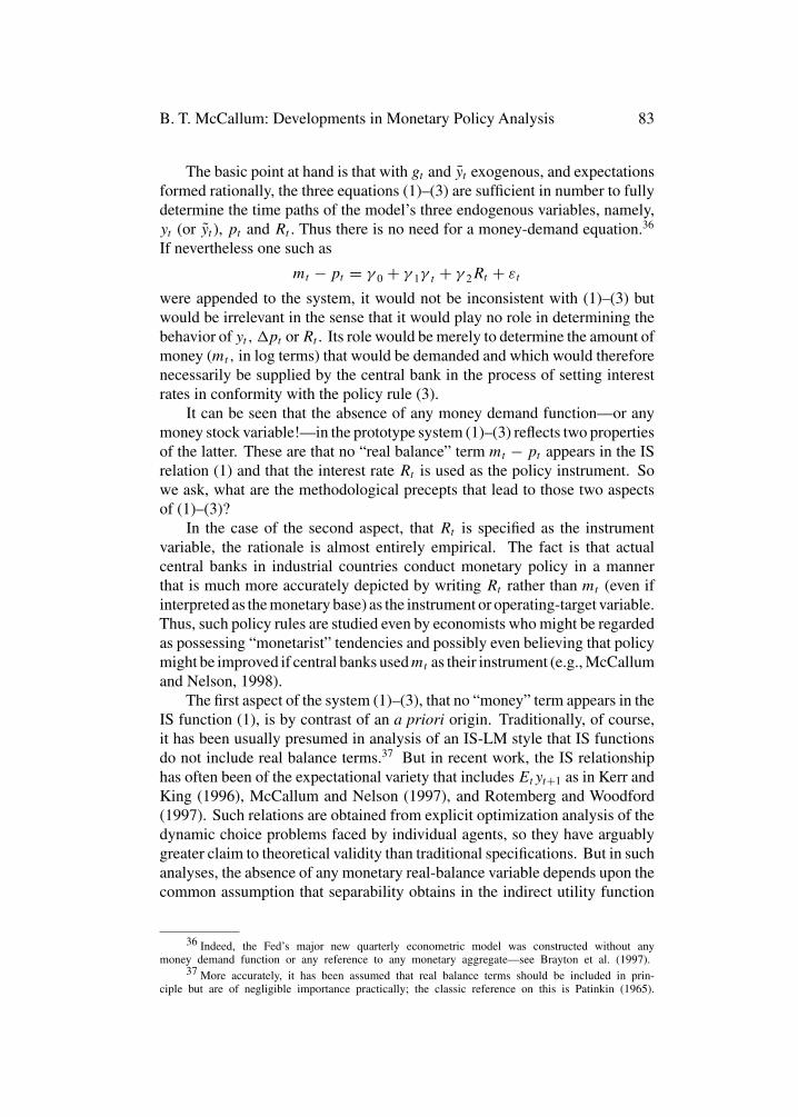
B. T. McCallum: Developments in Monetary Policy Analysis 83
The basic point at hand is that with gt and yt exogenous, and expectationsformed rationally, the three equations (1)–(3) are sufficient in number to fullydetermine the time paths of the model’s three endogenous variables, namely,yt (or yt ), pt and Rt. Thus there is no need for a money-demand equation.36
If nevertheless one such as
mt − pt = γ 0 + γ 1γ t + γ 2Rt + εt
were appended to the system, it would not be inconsistent with (1)–(3) butwould be irrelevant in the sense that it would play no role in determining thebehavior of yt , �pt orRt . Its role would be merely to determine the amount ofmoney (mt, in log terms) that would be demanded and which would thereforenecessarily be supplied by the central bank in the process of setting interestrates in conformity with the policy rule (3).
It can be seen that the absence of any money demand function—or anymoney stock variable!—in the prototype system (1)–(3) reflects two propertiesof the latter. These are that no “real balance” term mt − pt appears in the ISrelation (1) and that the interest rate Rt is used as the policy instrument. Sowe ask, what are the methodological precepts that lead to those two aspectsof (1)–(3)?
In the case of the second aspect, that Rt is specified as the instrumentvariable, the rationale is almost entirely empirical. The fact is that actualcentral banks in industrial countries conduct monetary policy in a mannerthat is much more accurately depicted by writing Rt rather than mt (even ifinterpreted as the monetary base) as the instrument or operating-target variable.Thus, such policy rules are studied even by economists who might be regardedas possessing “monetarist” tendencies and possibly even believing that policymight be improved if central banks usedmt as their instrument (e.g., McCallumand Nelson, 1998).
The first aspect of the system (1)–(3), that no “money” term appears in theIS function (1), is by contrast of an a priori origin. Traditionally, of course,it has been usually presumed in analysis of an IS-LM style that IS functionsdo not include real balance terms.37 But in recent work, the IS relationshiphas often been of the expectational variety that includes Etyt+1 as in Kerr andKing (1996), McCallum and Nelson (1997), and Rotemberg and Woodford(1997). Such relations are obtained from explicit optimization analysis of thedynamic choice problems faced by individual agents, so they have arguablygreater claim to theoretical validity than traditional specifications. But in suchanalyses, the absence of any monetary real-balance variable depends upon thecommon assumption that separability obtains in the indirect utility function
36 Indeed, the Fed’s major new quarterly econometric model was constructed without anymoney demand function or any reference to any monetary aggregate—see Brayton et al. (1997).
37 More accurately, it has been assumed that real balance terms should be included in prin-ciple but are of negligible importance practically; the classic reference on this is Patinkin (1965).

84 Federal Reserve Bank of Richmond Economic Quarterly
that reflects the transaction-facilitating properties of the medium of exchange(i.e., money). There is, however, no compelling theoretical basis for thatassumption, which is presumably made for analytical convenience. Indeed,it could be argued that separability is not very plausible. Accordingly, theabsence of any real balance term in (1), and the omission of monetary variablesfrom model (1)–(3), hinges on the presumption that nonseparabilities of therelevant type are quantitatively unimportant—i.e., that the marginal utility ofconsumption is (for a given rate of consumption) virtually independent of thelevel of real money balances. The justification for that presumption has notbeen explicitly discussed in the studies cited.
It has been mentioned that the NBER and Riksbank conferences featuredconsiderable agreement among participants concerning research strategy. Fur-thermore, Taylor (1998, 4–5) argues that there exists a fair amount of substan-tive agreement; specifically that model simulations at the NBER conference“show that simple policy rules work remarkably well in a variety of situations;they seem to be surprisingly good approximations to fully optimal policies”and “simple policy rules are more robust than complex rules across a varietyof models.” Also, “introducing information lags as long as a quarter does notaffect the performance of the policy rules by very much.” In addition, Tay-lor mentions other issues about which these studies do not reflect agreement,including: the value of interest-rate “smoothing” terms in the rules; whetherresponses should be geared to expected feature values rather than currently-observed values; and about measurement of potential or natural-rate output.
One area of disagreement among researchers concerns the distinction be-tween “optimal control” and “robustness” approaches for the design of mon-etary policy rules. For some analysts, the task of policy rule design is todevelop an appropriate macroeconomic model of the economy and then con-duct an optimal control exercise to determine what the best policy rule wouldbe for the economy in question. Neither step is trivial, but both representrather straightforward scientific problems. There would remain the task ofconvincing actual policy makers to implement this rule, of course, but that isa matter of persuasion rather than scientific investigation. Notable examplesof this approach are Feldstein and Stock (1994) and Svensson (1997). Toother economists, by contrast, a crucial feature of the policymaking processis the lack of professional agreement concerning the appropriate specifica-tion of a model suitable for monetary policy issues. Various members of thisgroup would emphasize different portions of a macro model,38 but to all in
38 My own candidate for the weakest component in a macroeconomic model is the price-adjustment (Phillips curve) sector. In McCallum (1999, fn. 14) the argument is stated as follows.“It is not just that the economics profession does not have a well-tested quantitative model of thequarter-to-quarter dynamics, the situation is much worse than that: we do not even have any basicagreement about the qualitative nature of the mechanism. This point can be made by mentioningsome of the leading theoretical categories, which include: real business cycle models; monetary
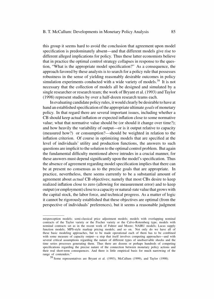
B. T. McCallum: Developments in Monetary Policy Analysis 85
this group it seems hard to avoid the conclusion that agreement upon modelspecification is predominately absent—and that different models give rise todifferent alleged implications for policy. Thus these latter economists believethat in practice the optimal control strategy collapses in response to the ques-tion, “What is the appropriate model specification?” As a consequence, theapproach favored by these analysts is to search for a policy rule that possessesrobustness in the sense of yielding reasonably desirable outcomes in policysimulation experiments conducted with a wide variety of models.39 It is notnecessary that the collection of models all be designed and simulated by asingle researcher or research team; the work of Bryant et al. (1993) and Taylor(1998) represent studies by over a half-dozen research teams each.
In evaluating candidate policy rules, it would clearly be desirable to have athand an established specification of the appropriate ultimate goals of monetarypolicy. In that regard there are several important issues, including whether aCB should keep actual inflation or expected inflation close to some normativevalue; what that normative value should be (or should it change over time?);and how heavily the variability of output—or is it output relative to capacity(measured how?) or consumption?—should be weighted in relation to theinflation criterion. Of course in optimizing models that are specified at thelevel of individuals’ utility and production functions, the answers to suchquestions are implicit to the solution to the optimal control problem. But againthe fundamental difficulty mentioned above intrudes in a crucial manner, forthese answers must depend significantly upon the model’s specification. Thusthe absence of agreement regarding model specification implies that there canbe at present no consensus as to the precise goals that are appropriate. Inpractice, nevertheless, there seems currently to be a substantial amount ofagreement about actual CB objectives; namely that most CBs desire to keeprealized inflation close to zero (allowing for measurement error) and to keepoutput (or employment) close to a capacity or natural-rate value that grows withthe capital stock, the labor force, and technical progress. As a matter of logicit cannot be rigorously established that these objectives are optimal (from theperspective of individuals’ preferences), but it seems a reasonable judgment
misperception models; semi-classical price adjustment models; models with overlapping nominalcontracts of the Taylor variety or the Fischer variety or the Calvo-Rotemberg type; models withnominal contracts set as in the recent work of Fuhrer and Moore; NAIRU models; Lucas supplyfunction models; MPS-style markup pricing models; and so on. Not only do we have all ofthese basic modeling approaches, but to be made operational each of them has to be combinedwith some measure of capacity output—a step that itself involves competing approaches—and withseveral critical assumptions regarding the nature of different types of unobservable shocks and thetime series processes generating them. Thus there are dozens or perhaps hundreds of competingspecifications regarding the precise nature of the connection between monetary policy actions andtheir real short-term consequences. And there is little empirical basis for much narrowing of therange of contenders.”
39 Some representatives are Bryant et al. (1993), McCallum (1999), and Taylor (1998).

86 Federal Reserve Bank of Richmond Economic Quarterly
that they probably provide an appropriate specification of CB macroeconomicgoals.
A related research-design issue that has attracted some attention involvesthe distinction between “instrument rules” and “target rules,” in the languageof Svensson (1997). Rules of the former type, exemplified by Taylor (1993)and presumed in my foregoing comments, specify period-by-period settingsof a controllable instrument variable as in equation (3) above. The second typeof rules, by contrast, specify target values for some variable or combination ofvariables that the CB can influence but not directly control, with these valuesobtained (at least in the work of Svensson) by optimal control exercises onthe basis of a designated model and objective function. Thus the specificationof a target rule amounts logically to the selection by the analyst of a modeland an objective function, whereas an instrument rule reflects the analyst’shypothesis that the CB would (whatever its model and objectives) achievesatisfactory results if it were to implement the rule.40
It has been emphasized that models represented by the system (1)–(3)specify slowly adjusting price levels. Thus central-bank policy actions, rep-resented by changes in Rt , typically have effects on real output, yt . It is ofsome importance to ask, then, what is the scientific justification for modelsof this type in preference to ones (including RBC models) in which monetarypolicy actions have no systematic effects on real variables. Is it theory orempirical evidence that indicates that prices are sticky and monetary policyable to influence output?41
Here the argument is much the same as that of Section 2 above—the answermust be empirical evidence since neoclassical theory certainly does not entailprice stickiness. But then the question becomes, what type of evidence hasindicated strongly and clearly that sticky prices and monetary effects on realvariables are a feature of actual economies? For it is unclear how to lookfor the former, empirically, and there is no shortage of empirical studies thatfail to find major effects of the latter type (e.g., Eichenbaum and Singleton1986). Regarding sticky prices per se there is some survey evidence providedby Blinder (1994) and studies of particular commodities by others but it ismy impression that most analysts have judged these to be non-compelling.More influential, I believe, has been the perception that sharp major changesin monetary policy conditions (e.g., in the United States during 1981) have infact had major real effects in the same direction, together with the belief thatprice stickiness provides the most satisfactory means of rationalizing that fact.
40 There is also a major controversy as to whether a CB can implement a rule of the“committed” or “non-discertionary” type. Since my own affirmative position on this issue (e.g.,McCallum 1999) is somewhat unorthodox, I propose not to discuss it in the present paper.
41 There is small but significant school of thought that attributes real effects of policy tofinancing constraints in flexible-price models, e.g., Christiano and Eichenbaum (1995). Discussionof this position is beyond the scope of the present paper.

B. T. McCallum: Developments in Monetary Policy Analysis 87
Ironically, the empirical study that has probably attracted the most support forthis viewpoint is Romer and Romer (1989), a study that, like Hoover and Perez(1994), I find rather unsatisfactory.42
One source of difficulty in formal empirical studies of monetary policyeffects on real variables has been the common practice of focusing attentionon real responses to policy innovations—i.e., unexpected components —invector autoregression (VAR) studies. Although Christiano, Eichenbaum, andEvans (1998) have reported effects of this type in an extensive study, theyare not quantitatively large in many VAR studies. But the VAR approachseems inherently to miss the major effects, because the measured innovationcomponent of policy-variable fluctuations is extremely small relative to thesystematic component in terms of variability. Thus, for example, the system-atic component’s variability is about 16 times as large as for the innovationcomponent in an estimated interest rate policy rule for the U.S., 1955–1996(quarterly data). One way of making the relevant point is by consideration ofan extreme case. Suppose that a central bank’s policy rule is activist but en-tirely systematic, i.e., is devoid of random components. Then a well-designedVAR study would attribute no importance to monetary policy in affectingoutput—or inflation!—although it could be that the systematic component ofpolicy was in fact very important.
A related point concerns the way in which empirical evidence works inpersuading specialists in monetary economics (and, probably, other areas). Inthat regard it is almost never the case that an analyst’s view on some importanthypothesis is crucially dependent upon the results of a formal econometricstudy—no single study is decisive. This is in part because conclusions aboutcrucial properties of macroeconomic systems almost always require identifica-tion of structural parameters in a well-specified model, yet both identificationand “correct specification” are exceedingly difficult to achieve in the macroe-conomic context, for there is usually some highly dubious feature of anymanageable model. Instead, it is the cumulative effect of several econometricstudies and/or various bits of evidence obtained in more informal ways, alltaken together, that is usually persuasive to an analyst.
This section has argued that monetary policy analysis, like macroeco-nomics more generally and the practice of monetary policy, has been signif-icantly influenced over the last 25 years by both theoretical and empiricaldevelopments. That such is the case is certainly desirable, I would think.
42 It is obvious that the Romer and Romer (R&R) dummy variable is not exogenous, for itreflects actions taken in response to recently-prevailing macroeconomic conditions. Thus my ownsummary statement (McCallum 1994, 334) is that their study differs from previous attempts tomeasure monetary policy effects primarily as follows: “the R&R dummy reflects changes in onlyone direction, does not reflect the intensity of policy actions, and is based on statements ratherthan actions. Thus one is led to wonder how use of this dummy, instead of a traditional measure,constitutes an improvement over prior practice.”
88 Federal Reserve Bank of Richmond Economic Quarterly
Indeed, there is an important sense in which significant scientific progress in-evitably requires both theoretical and empirical inputs. Evidence is necessary,obviously, because theories with content may by construction be untrue, i.e.,grossly inconsistent with relevant facts. But theory too is necessary, for onecan only make sense of facts and measurements within the disciplining contextof a theoretical structure that gives these facts some coherence and delineateswhat is and is not relevant, etc.
5. COINTEGRATION AND MONETARY ANALYSIS
In this section, I would like to take up an issue that is highly pertinent tothis paper’s theme although it failed to find a place in the above evolutionarydiscussion. This issue concerns a claim, which appears occasionally in theliterature, to the effect that a failure of real money balances, real income, andnominal interest rates to be cointegrated implies the absence of any long-run relationship of the type that is necessary for the validity of traditionalmonetary economics. Cuthbertson and Taylor (1990, 295), for example, haveexpressed the claim as follows: “If the concept of a stable, long-run moneydemand function is to have any empirical content whatsoever, thenmt [i.e., logmoney]. . . must be cointegrated with log prices, log income, and interest rates.”Engle and Granger (1987) presented evidence contrary to the cointegrationhypothesis; several other researchers have reached the opposite conclusionbut only after accepting the presumption that cointegration is necessary forstandard monetary analysis.
My objective here is to argue that this presumption is basically mistaken.Of course there is a technical sense in which it is correct: ifmt −pt, yt andRtare all integrated (difference-stationary) of order one43 but not cointegrated,then the disturbance entering any linear relation among them must by definitionbe nonstationary, somt −pt and any linear combination of yt and Rt can driftapart as time passes. But it is highly misleading to conclude that in anypractical sense a long-run relationship is therefore nonexistent. The followingargument is entirely interpretive; it includes no suggestion of technical errorin the literature discussed. But that does not diminish its importance.
To develop the argument, let us consider again the example of a tradi-tional money demand function of the form (4). Suppose that mt − pt, yt andRt are all I(1) variables and that each has been processed by the removal ofa deterministic trend. Then the cointegration status of relationship (4) depends
43 A time-series variable is integrated of order one, written I(1), if it must be differencedonce to obtain a variable that is covariance stationary. This will be the case for an ARMA variableif its autoregressive parameter has a unit root.
B. T. McCallum: Developments in Monetary Policy Analysis 89
upon the properties of the disturbance term εt : if its process is of the difference-stationary type that includes a unit AR root, then the variables in (4) will notbe cointegrated.
But the traditional view of money demand theory, as represented by thestudies cited above, provides no reason for believing that εt would instead betrend stationary (i.e., would possess no AR unit root component). Indeed, itwould seem almost to suggest the opposite—for the theoretical rationale for (4)is built upon the transaction-facilitating function of money, but the technologyfor effecting transactions is constantly evolving. And since technical progresscannot be directly measured by available variables, the effects of technicalchange (not captured by a deterministic trend) show up in the disturbance term,εt . But the nature of technological progress is such that changes (shocks) aretypically not reversed. Thus one would expect a priori there to be an importantpermanent component to the εt process, making it one of the integrated type—and thereby making mt − pt not cointegrated with yt and Rt .
In such a case, however, the “long-run” messages of traditional monetaryanalysis could easily continue to apply. Provided that the magnitude of thevariance of the innovation in εt is not large in relation to potential magnitudesof�mt values, it will still be true that inflation rates will be principally deter-mined, over long periods of time, by money growth rates. And even withoutthat proviso, long-run monetary neutrality may still prevail, superneutralitymay be approximately but not precisely valid, etc. That the disturbance εtis of the difference-stationary class is simply not a source of embarrassmentor special concern for supporters of the traditional theory of money demand,some of whom have estimated money demand relations like (4) after assumingthat εt is a pure random walk!44
6. CONCLUSION
The picture painted in the preceding discussion is one that attributes majorchanges in the analysis and practice of monetary policy over the years 1973–1998 to a combination of theoretical and empirical influences. This is not avery dramatic conclusion; indeed, one might say that it is almost empty. Itwould be possible to add a bit of debatable content, by asserting that the mixtureof influences has been reasonably appropriate—about the right amount oftheory and empirics—but I would not feel comfortable in doing so. Partly thatis because I would have preferred that models with complete price flexibility
44 More generally, I would a priori expect cointegration among basic variables—ones thatenter utility or production functions, not their differences—to be quite rare. for behavioral rela-tions typically include disturbance terms that represent unobservable (and thus omitted) variables,which include shocks to preferences and technology. But these shocks would seem likely to in-clude significant random-walk components, as argued above. Thus disturbance terms in behavioralrelations should, according to this argument, typically possess unit-root components.
90 Federal Reserve Bank of Richmond Economic Quarterly
had not been quite so dominant during the years (say) 1982–1992, although thesurge of work with sticky price models in recent years may have largely madeup for their previous neglect. But an equally important reason stems from thequestion: what type of evidence could be presented in support of a “reasonablyappropriate” contention? Unfortunately, I know of no satisfactory way ofmaking such a determination, especially since most influential studies involvea blend of theory and evidence. For example, the rather abstract theoreticalanalysis of Lucas (1972a) was not actually devoid of empirical content in thesense that its theorizing was specifically designed to rationalize a set of broadfacts that were (and are) of genuine, fundamental importance. Consequently,I am left with the rather limp conclusion with which this paragraph began.
In conclusion, then, it may be appropriate to add the opinion that thecurrent state of monetary economics is not as highly unsatisfactory as hasbeen claimed over the past decade or so by various commentators at confer-ences and seminars. The type of claim that I have in mind does not oftenmake it into print, so I cannot provide citations, but I am confident that manyreaders can supply examples from their own experiences. In any event, thestate of monetary economics seems to me to be about as healthy as that ofeconomic analysis in general. The contrary opinion is rather widely heldfor three reasons, I would suggest, none of which is sound. First, much ofthe negative opinion has been put forth by economists who are themselvesproponents of an entirely unsatisfactory theory of money demand, one in-volving overlapping generations models in which the asset termed “money”plays no role as a (transaction-facilitating) medium of exchange. Since thisrole provides the defining characteristic of money, as distinct from other as-sets, it is not surprising that proponents of such a theory would find it un-satisfactory. Second, rather inconsequential differences among proponentsof the transaction-facilitating approach to money demand theory—e.g., cash-in-advance, money-in-utility function, shopping time, or transaction-cost-in-budget constraint models—have tended to obscure the fundamental similarityof principles and implications among the variants of this approach. Third, theprofession’s poor level of understanding of the precise nature of the dynamicconnection between monetary and real variables—i.e., of price adjustmentrelations—has tended to reflect discredit upon monetary economics, althoughthis relation belongs to the realm of macroeconomics more broadly. In thatregard, moreover, it is an illusion to believe that macroeconomics is itself inpoor condition in relation to microeconomics, an illusion generated by thefact that applied macro features a much more ambitious agenda than appliedmicro—the understanding of quarter-to-quarter dynamic movements in vari-ables rather than just steady-state values. Correcting for that difference, theextent of disagreement seems about the same in the two sub-disciplines.

B. T. McCallum: Developments in Monetary Policy Analysis 91
REFERENCES
Alogoskoufis, G. L., and Smith, R. (1991) “The Phillips curve, thepersistence of inflation, and the Lucas critique,” American EconomicReview 81: 1254–75.
Altug, S. (1989) “Time-to-build and aggregate fluctuations,” InternationalEconomic Review 30: 889–920.
Axilrod, S. H. (1983) “A comment on Brunner and Meltzer,” Carnegie-Rochester Conference Series 18: 105–12.
Barro, R. J. (1977) “Unanticipated money growth and unemployment in theUnited States,” American Economic Review 67: 101–15.
Barro, R. J., and Gordon, D. B. (1983) “A positive theory of monetary policyin a natural rate model,” Journal of Political Economy 91: 589–610.
Basu, S. (1996) “Procyclical productivity: increasing returns or cyclicalutilization,” Quarterly Journal of Economics 111: 719–51.
Bernanke, B. S., and Mishkin, F. S. (1997) “Inflation targeting: A newframework for monetary policy?” Journal of Economic Perspectives 11:97–116.
Blinder, A. S. (1994) “On sticky prices: academic theories meet the realworld,” Monetary Policy, ed. N.G. Mankiw. Chicago: University ofChicago Press.
Brayton, F., Levin, A., Tryon, R., and Williams, J. C. (1997) “The evolutionof macro models at the Federal Reserve Board,” Carnegie-RochesterConference Series on Public Policy 47: 43–81.
Broaddus, A., and Goodfriend, M. (1984) “Base drift and the longer-rungrowth of M1: Experience from a decade of monetary targeting,” FederalReserve Bank of Richmond Economic Review 70 (Nov./Dec.): 3–14.
Brunner, K., and Meltzer, A. H. (1983) “Strategies and tactics for monetarycontrol,” Carnegie-Rochester Conference Series 18: 59–104.
Bryant, R. C., Hooper, P., and Mann, C. L. (1993) Evaluating PolicyRegimes: New Research in Empirical Macroeconomics. Washington:Brookings Institution.
Burns, A. (1979) “The real issues of inflation and unemployment,” FederalReserve Readings on Inflation. Federal Reserve Bank of New York.
Calvo, G. A. (1983) “Staggered prices in a utility prices in a utilitymaximizing framework,” Journal of Monetary Economics 12: 383–98.

92 Federal Reserve Bank of Richmond Economic Quarterly
Christiano, L. J., and Eichenbaum, M. (1995) “Liquidity effects, monetarypolicy, and the business cycle,” Journal of Money, Credit, and Banking27: 1113–36.
Christiano, L. J., Eichenbaum, M., and Evans, C. L. (1998) “Monetarypolicy shocks: What have we learned and to what end?” NBER Workingpaper 6400. Forthcoming in Handbook of Macroeconomics, ed. J. B.Taylor and M. Woodford. Amsterdam: North Holland.
Cogley, T., and Nason, J. M. (1995) “Output dynamics in real-business cyclemodels,” American Economic Review 85: 492–511.
Cuthbertson, K., and Taylor, M. P. (1990) “Money demand, expectations, andthe forward-looking model,” Journal of Policy Modeling 12: 289–315.
Eichenbaum, M., and Singleton, K. J. (1986) “Do equilibrium real businesscycle theories explain postwar U.S. business cycles?” NBERMacroeconomic Annual 1986. Cambridge, MA: MIT Press.
Engle, R. F., and Granger, C. W. J. (1987) “Co-integration and errorcorrection: Representation, estimation, and testing,” Econometrica 55:251–76.
Ericsson, N., and Irons, J. (1995) “The Lucas critique in practice: Theorywithout measurement,” in Macroeconometrics: Developments, Tensions,and Prospects, ed. by K. D. Hoover. Boston: Kluwer Academic Press,263–312.
Evans, C. L. (1992) “Productivity shocks and real business cycles,” Journalof Monetary Economics 29: 191–208.
Feldstein, M., and Stock, J. H. (1994) “The use of a monetary aggregate totarget nominal GDP,” in Monetary Policy, ed. N. G. Mankiw. Chicago:University of Chicago Press.
Friedman, M. (1966) “Comments,” in Guidelines, Informal Controls, and theMarketplace, ed. G. P. Schultz and R. Z. Aliber. Chicago: University ofChicago Press.
. (1968) “The role of monetary policy,” American EconomicReview 58: 1–17.
Fuhrer, J. C. (1997) “The (un)importance of forward-looking behavior inprice specifications,” Journal of Money, Credit, and Banking 29: 338–50.
. (1995) “The persistence of inflation and the cost ofdisinflation,” New England Economic Review Jan/Feb: 3–16.
, and Moore, G. R. (1995) “Inflation persistence,” QuarterlyJournal of Economics 109: 127–59.

B. T. McCallum: Developments in Monetary Policy Analysis 93
Gali, J. (1997) “Technology, employment, and the business cycle: Dotechnology shocks explain aggregate fluctuations?” NBER WorkingPaper 5721.
Goodfriend, M. (1997) “Monetary policy comes of age: A 20th centuryodyssey,” Federal Reserve Bank of Richmond Economic Quarterly 83(Winter): 1–22.
Goodfriend, M., and King, R. E. (1997) “The new neoclassical synthesis andthe role of monetary policy,” NBER Macroeconomics Annual 1997:231–82.
Gordon, R. J. (1970) “The recent acceleration of inflation and its lessons forthe future,” Brookings Papers on Economic Activity, No. 1: 8–41.
. (1975) “The impact of aggregate demand on prices,”Brookings Papers on Economic Activity, No. 3: 613–62.
Haldane, A. G., ed. (1995) Targeting Inflation. Bank of England.
Hall, R. E. (1978) “Stochastic implications of the life-cycle-permanentincome hypothesis: theory and evidence,” Journal of Political Economy86: 971–87.
Hansen, L. P., and Singleton, K. J. (1982) “Generalized instrumentalvariables estimation of nonlinear rational expectations models,”Econometrica 50: 1269–86.
Hendry, D. F. and Ericsson, N. R. (1991) “Modeling the demand for narrowmoney in the United Kingdom and the United States,” EuropeanEconomic Review 35: 833–86.
Hoover, K. D. (1995) “Facts and artifacts: calibration and the empiricalassessment of real business cycle models,” Oxford Economic Papers 47:24–44.
Hoover, K. D., and Perez, S. J. (1994) “Money may matter, but how couldyou know?” Journal of Monetary Economics 34: 89–100.
Kerr, W. and King, R. G. (1996) “Limits on interest rate rules in the IS-LMmodel,” Federal Reserve Bank of Richmond Economic Quarterly 82(Spring): 47–75.
King, R. E. (1990) “Money and business cycles,” Working Paper.Forthcoming in Journal of Monetary Economics.
King, R. E., and Watson, M. W. (1994) “The post-war U.S. Phillips curve: arevisionist econometric history,” Carnegie-Rochester Conference Series41: 157–219.
Kydland, F. E., and Prescott, E. C. (1980) “A competitive theory offluctuations and the feasibility of stabilization policy,” in Rational

94 Federal Reserve Bank of Richmond Economic Quarterly
Expectations and Economic Policy, ed. S. Fischer. Chicago: Universityof Chicago Press.
. (1982) “Time to build and aggregate fluctuations,”Econometrica 50: 1345–70.
. “The workweek of capital and its cyclical implications,”Working paper.
Leiderman, L., and Svensson, L. E. O., eds. (1995) Inflation Targets.London: Centre for Economic Policy Research.
Litterman, R. B., and Weiss, L. (1989) “Money, real interest rates, and output:a reinterpretation of postwar U.S. data,” Econometrica 53: 129–56.
Lucas, R. E., Jr. (1972a) “Expectations and the neutrality of money,” Journalof Economic Theory 4: 103–24.
. (1972b) “Econometric testing of the natural-ratehypothesis,” in The Econometrics of Price Determination, ed.O. Eckstein. Washington, D.C.: Board of Governors of the FederalReserve System.
. (1973) “Some international evidence on output-inflationtradeoffs,” American Economic Review 63: 326–34.
. (1975) “An equilibrium model of the business cycle,”Journal of Political Economy 83: 1113–44.
. (1976) “Econometric policy evaluation: a critique,”Carnegie-Rochester Conference Series 1: 19–46.
. (1988) “Money demand in the United States: a quantitativereview,” Carnegie-Rochester Conference Series 29: 137–67.
Mankiw, N. G., Rotemberg, J. J., and Summers, L. (1985) “Intertemporalsubstitution in macroeconomics,” Quarterly Journal of Economics 100:225–51.
Marschak, J. (1953) “Economic measurements for policy and prediction,” inStudies in Econometric Method, ed. W. C. Hood and T. J. Koopmans.New York: John Wiley.
McCallum, B. T. (1976) “Rational expectations and the natural ratehypothesis: some consistent estimates,” Econometrica 44: 43–52.
. (1980) “Rational expectations and macroeconomicstabilization policy,” Journal of Money, Credit, and Banking 12: 716–46.
. (1986) “On ‘real’ and ‘sticky-price’ theories of thebusiness cycle,” Journal of Money, Credit, and Banking 18: 397–414.
B. T. McCallum: Developments in Monetary Policy Analysis 95
. (1989) “Real business cycle models,” in Modern BusinessCycle Theory, ed. R. J. Barro. Cambridge, MA: Harvard UniversityPress.
. (1994) “Comment on ‘Federal Reserve Policy: Cause andEffect’ by M. D. Shapiro,” in Monetary Policy, ed. N. G. Mankiw.Chicago: University of Chicago Press for NBER.
. (1999) “Issues in the design of monetary policy rules,” inHandbook of Macroeconomics, ed. J. B. Taylor and M. Woodford.Amsterdam: North-Holland Pub. Co.
McCallum, B. T., and Goodfriend, M. S. (1987) “Demand for money:theoretical studies,” in The New Palgrave, ed. J. Eatwell, M. Milgate,and P. Newman. New York: Stockton Press.
McCallum, B. T., and Nelson, E. (1997) “An optimizing IS-LM specificationfor monetary policy and business cycle analysis,” NBER Working paper5875. Forthcoming in Journal of Money, Credit, and Banking 31.
. (1998) “Nominal income targeting in an open-economymaximizing model,” NBER Working paper 6675.
Nelson, C. R., and Plosser, C. I. (1982) “Trends and random walks inmacroeconomic time series,” Journal of Monetary Economics 10:139–62.
Nelson, E. (1998) “Sluggish inflation and optimizing models of the businesscycle,” Journal of Monetary Economics 42: 303–22.
Patinkin, D. (1965) Money, Interest, and Prices, second ed. New York:Harper & Row.
Phelps, E. S. (1967) “Phillips curves, expectations of inflation, and optimalunemployment overtime,” Economica 34: 254–81.
Prescott, E. S. (1986) “Theory ahead of business cycle measurement,”Carnegie-Rochester Conference Series 25: 11–44.
Romer, C. D., and Romer, D. (1989) “Does monetary policy matter? A newtest in the spirit of Friedman and Schwartz,” NBER MacroeconomicsAnnual 1989: 121–70.
Rotemberg, J. J. (1982) “Monopolistic price adjustment and aggregateoutput,” Review of Economic Studies 44: 517–31.
Rotemberg, J. J., and Woodford, M. (1997) “An optimization basedeconometric framework for the evaluation of monetary policy,” NBERMacroeconomics Annual 1997: 297–345.
Sargent, T. J. (1971) “A note on the accelerationist controversy,” Journal ofMoney, Credit, and Banking 3: 50–60.

96 Federal Reserve Bank of Richmond Economic Quarterly
. (1973) “Rational expectations, the real rate of interest, andthe natural rate of unemployment,” Brookings Papers on EconomicActivity, No. 2: 429–72.
Sargent, T. J., and Wallace, N. (1975) “’Rational’ expectations, the optimalmonetary instrument, and the optimal money supply role,” Journal ofPolitical Economy 83: 241–54.
Sims, C. A. (1980) “A comparison of interwar and postwar business cycles:monetarism reconsidered,” American Economic Review Papers andProceedings 70: 250–57.
Solow, R. M. (1969) Price Expectations and the Behavior of the Price Level.Manchester: Manchester University Press.
Svensson, L. E. O. (1997) “Inflation forecast targeting: implementing andmonitoring inflation targets,” European Economic Review 41: 1111–46.
Taylor, J. B. (1980) “Aggregate dynamics and staggered contracts,” Journalof Political Economy 88: 1–23.
. (1989) “Monetary policy and the stability ofmacroeconomic relationships,” Journal of Applied Econometrics 4:S161–78.
. (1993) “Discretion versus policy rules in practice,”Carnegie-Rochester Conference Series 39, 195–214.
. (1996) “How should monetary policy respond to shockswhile maintaining long-run price stability—conceptual issues,” inAchieving Price Stability, Federal Reserve Bank of Kansas City.
. (1998) “The robustness and efficiency of monetary policyrules as guidelines for interest rate setting by the European CentralBank,” Working paper.
Tobin, J. (1969) “Discussion,” Inflation: Its Causes, Consequences, andControl, ed. S. W. Rousseas. New York: New York University.
Walsh, C. E. (1998) Monetary Theory and Policy. Cambridge, MA: MITPress.
Walters, A. A. (1971) “Consistent expectations, distributed lags, and thequantity theory,” Economic Journal 81: 273–81.
Watson, M. W. (1993) “Measures of fit for calibrated models,” Journal ofPolitical Economy 101: 1011–41.
Woodford, M. (1995) “Price-level determinacy without control of amonetary aggregate,” Carnegie-Rochester Conference Series 43: 1–46.