german tourism demand for the czech ... - wur e-depot home
TRANSCRIPT

German tourism demand for the Czech Republic:
A cointegration analysis
Author: Jiri Lukes
Registration number: 870609533040
Supervisor: dr.ir. Monique Mourits
Examiner: prof.dr.ir. Henk Hogeveen
Chair group: Business Economics
Course code: BEC-80433
Date: 14th July 2016


i
Abstract
Germans create the largest group of tourists visiting the Czech Republic. As indicated by literature,
income, relative prices, transportation costs and exchange rates are the most used explanatory
variables for estimating the tourism demand. The aim of this thesis is to define the influence of these
exogenous factors on German tourism demand for the Czech Republic using a cointegration analysis
and to evaluate the possible impacts of these exogenous variables on the number of German tourists
in the future. Having such a forecast on tourism demand as accurate as possible is essential for
efficient planning of tourism-related businesses
The study used data on prices of oil, German GDP, the consumer price index between the Czech
Republic and German (CPI) and the exchange rate in the form of quarterly time series for the period
1999 – 2014. The Augmented Dickey Fuller test was used to test the stationarity of all time series and
the order of integration among the selected variables. It proved that all data had a non-stationary
character and that the time series became stationary after their first differences. Then Johansen´s
procedure was carried out to indicate the presence of any cointegrative relationship among the
explaining, which was confirmed by the Trace Test. The Vector Error Correction model was
subsequently used to examine long-run causality and short-term relationship between the German
tourism demand and the explanatory variables.
Results show that on the short run a change in CPI or oil price has a significant effect (P<0.05) on the
arrival of German tourists. The error correction term was estimated as -0.29, indicating that a
deviation of German tourists in the Czech Republic from a long-run equilibrium will be corrected by
29% in the next quarter. On the long run all evaluated variables , except of GDP, are significantly
influencing demand (P<0.1). An Impulse Response analysis indicated that the impact of the shocks of
the individual variables on tourism demand within the coming 2,5 years is not expected to be strong
from which it can be concluded that the German tourism demand during that period for the Czech
Republic is rather robust.
Key words: tourism demand, GDP, exchange rate, oil, consumer price index, cointegration analysis,
error correction model

ii
Acknowledgements
I would like to thank to my supervisor dr.ir. Monique Mourits for the continual help that she
provided to me. Thank you very much for all the meetings and discussions that we had. Certainly
without your help I would not be able to finish this paper.
Second I would like to thank to my girlfriend, Leona, for helping me during this long period of my
studying, for giving me motivations to pass that and for being tolerant during hard times.
The last but not least I would like to express gratitude to my parents who gave me a chance to study
at university and supported me the whole time without any hesitations.
iii
Table of Contents Abstract ................................................................................................................................................ i
Acknowledgements ..............................................................................................................................ii
List of figures and tables...................................................................................................................... iv
1 Introduction ..................................................................................................................................... 1
2 Descriptive analysis; tourism in the Czech Republic ....................................................................... 3
2.1 The changes in the Czech Republic after 1989 ........................................................................ 3
2.2 Changes in tourism demand .................................................................................................... 4
2.3 The structure of tourism demand in the Czech Republic ........................................................ 6
3 Materials and Methods ................................................................................................................... 9
3.1 Theoretical framework ............................................................................................................ 9
3.2 Definition tourism demand ................................................................................................... 10
3.3 Data ....................................................................................................................................... 13
3.4 Methods ................................................................................................................................ 15
4 Results ........................................................................................................................................... 21
4.1 Cointegration analysis ........................................................................................................... 21
4.2 Impulse Response and Forecast error variance decomposition ........................................... 25
4.3 Forecast error variance decomposition ................................................................................ 27
5 Discussion and Conclusion ............................................................................................................ 29
6 References ..................................................................................................................................... 33
7 Appendices .................................................................................................................................... 37
7.1 Appendix A ............................................................................................................................ 37
7.2 Appendix B Forecast .............................................................................................................. 49
7.3 Appendix C ............................................................................................................................. 53
........................................................................................................................................................... 53
iv
List of figures and tables
Figure 1 Number of tourists in thousands visiting Czech Republic through time (CSO, 2016) ............... 5
Figure 2 Development of German GDP and oil prices between 1999 and 2014 (Source: Eurostat,
Statista).................................................................................................................................................. 13
Figure 3 Development of explanatory variables between 1999 and 2014.(Source: CSO,Eurostat) ..... 14
Figure 4 Response of LN_ARRIVALS to LN_OIL...................................................................................... 25
Figure 5 Response of LN_ARRIVALS to LN_GDP .................................................................................... 26
Figure 6 Response of LN_ARRIVALS to LN_CPI_CZK_GER ..................................................................... 26
Figure 7 Response of LN_ARRIVALS to LN_CZK_EUR ............................................................................ 26
Figure 8 Variance Decomposition of LN_ARRIVALS .............................................................................. 28
Table 1 The structure of tourism demand in the Czech Republic in the years 2000 and 2013 (CSO,
2016) ........................................................................................................................................................ 7
Table 2 Basic descriptions on quarterly number of arrivals and the quarterly values on GDP, tourism
prices, exchange rate and travelling costs during the period 1999-2014 ............................................. 14
Table 3 Testing non-stationary time series ............................................... Error! Bookmark not defined.
Table 4 Testing stationary time-series .................................................................................................. 21
Table 5 Unrestricted Cointegration Rank Test (Trace) Johansen cointegration test ............................ 22
Table 6 Long-term Vector Error Correction Model ............................................................................... 23
Table 7 Estimated Short-run Error Correction Model ........................................................................... 24
Table 8 Wald Test statistics ................................................................................................................... 24
Table 9 Variance Decomposition of LN_ARRIVALS ................................................................................ 27
1
1 Introduction
Nowadays tourism is one of the fastest growing industries in the world. According to the statistics of
the World Tourism organization UNWTO about 392 million of visitors travelled to Europe in 2000,
after which during the following 9 years the amount of tourists increased by 17% to 459 million
(UNWTO, 2010) to 582 million in 2014(UNWTO, 2014). Due to this increasing number of tourists and
the amount of money they spend in the selected countries, tourism has become one of the major
contributors to the recovery of European economic crisis and it creates a fundamental part of
countries’ budgets (UNWTO, 2014).
The increase of tourists is not only visible in Western Europe but it was relatively even higher in
Eastern Europe. From 2010 to 2013 the increase in the amount of tourists visiting Eastern Europe
was almost 29%, from 98.4 million to 127 million (UNWTO, 2013).
The Czech Republic belongs among those post-communist countries of Eastern Europe which
popularity in tourism has been growing fast after the collapse of the Eastern Bloc in 1989. Currently
the number of incoming tourists (people arriving to the country) prevails to the outgoing ones.
Tourism provides economic, social and environmental contributions to the state. From the economic
point of view tourism contributes to the governmental budget in the form of revenues, foreign
exchange earnings, job opportunities and many other business chances. The importance of the
incoming tourism in the Czech Republic grows every year. The share of tourism on the GDP has been
constantly growing since 1989 with the exception of the economic crisis that hit the European
economy from 2009 to 2012. In 2014 this share created about 6.8% of GDP (CSÚ, 2015). Tourism
positively effects the employment rate as well and in 2014 it even made 4.6% share on the total
employment rate generating 248 500 jobs (CSÚ, 2015).
In the Czech Republic the most fundamental group of tourists is represented by Germans. There are
a few reasons for that, firstly the travel distance between the two countries and secondly the price
differences that makes the Czech Republic more affordable. In 2000 the number of Germans
travelling to the Czech Republic represented more than 42% of all incoming tourists (CSÚ, 2000).
Insight in the tourism demand is crucial for all tourism related businesses such as airlines, tour
operators, all types of accommodation, transportation companies and of course shop owners selling
goods related to tourism. These establishments are highly interested in the demand for their goods
2
and services and in the estimation of future tourism demand as this is fundamental for their strategic
planning of their businesses.
Tourism demand analysis is also significant for understanding the importance of different economic
determinants of demand, information which is relevant for tourism policy makers such as Czech
Tourism - National Tourism Board or Czech Ministry of Regional Development. Measuring the
tourism demand is useful for evaluating the share of tourism industry on the whole national
economy and to provide necessary information for the optimal use and efficient resource allocation.
What is more, the strategic tourism planning requires full-understanding of factors that have impact
on the tourists´ choice of destination, different journeys and trips and of course understanding the
short and long-term forecasting (Loannides and Debbage, 1998).
According to Song and Li (2008) the most explanatory data with respect to tourism demand are
related to arrivals´ income, tourism prices adapted by exchange rates and travelling costs.
The main purpose of this thesis is to define the influence of these exogenous factors on German
tourism demand for the Czech Republic using a cointegration analysis and to evaluate the possible
impacts of these exogenous variables on the number of German tourists in the future. Having such a
forecast on tourism demand as accurate as possible is essential for efficient planning of tourism-
related businesses as mentioned above.
In order to accomplish this objective, the following research questions have been explored
What has been the development of tourism in the Czech Republic after becoming a
parliamentary republic in 1989?
To what extent is the German tourism demand in the Czech Republic affected by the factors -
income, tourism prices, exchange rate and travelling costs?
How will the German tourism demand for the Czech Republic be influenced by these selected
variables in the nearby future?

3
2 Descriptive analysis; tourism in the Czech Republic
2.1 The changes in the Czech Republic after 1989
The period between the end of the 80´s and the early 90´s was accompanied by revolutionary waves
in Central and Eastern Europe that suffered under the Communist regime. These revolutions resulted
in the end of the communist government and meant a new phase in history. The Czech Republic was
not an exception and the year 1989 when the so called Velvet Revolution occurred, meant a huge
progress in political structures of the state. This revolution ended 41 years of communist rule in the
Czech Republic and meant a transition of the state power to a parliamentary republic.
After 1989 the Czech Republic recorded a huge development in many sectors of national economy
thanks to crucial changes – especially the opening of the boarders and the change from a central
planned economy system to a market oriented economy (Vanek and Mucke, 2015). During the first
years of the existence of the Czech Republic as a democratic country, many structural changes
occurred, like price deregulations, privatization and liberalization of international trade and currency
exchange that caused a decline of economic growth and an increase of inflation. This negative side of
the transformation caused a reduction of purchasing power of the Czechs. On the other hand the
privatization process helped to change the ownerships of tourism establishments and the way how
people use their leisure time (Tittelbachova, 2011).
After the conversion to a parliamentary republic in 1989 the organization of tourism in the Czech
Republic was fundamentally changed into a modern and democratic system on central, regional or
local level. New tools and subjects of tourism were created - state and territory politics, their
concepts and programs of tourism development including allocation of limited financial tools,
organization and activities in touristic regions and areas, re-foundation of touristic clubs, new roles of
cities and towns related to supporting tourism, modern education of tourism in high schools and
universities (especially management and marketing) and finally significant support of tourism
development from different funds of EU. In 1990 the new Ministry of trade and tourism in the Czech
Republic was founded. Main tasks of this Ministry consist of coordination, national promotion abroad
and of distributing subsidies from European Union and National funds related to tourism.
The most important changes related to the private sector were initiated by the Small privatization
law in 1991, which helped to return nationalized establishments, especially the basic tourism
4
enterprises, to the hands of business subjects – mainly to private small and middle entrepreneurs.
These enterprises were mostly related to small accommodations although many of them were in
desolated conditions. This first step – the whole process of small privatization - took more than 15
years till 2006. As a result a huge number of business units – overnight accommodations, eating
enterprises and travel agencies - were created. Subsequently, a second step - the large privatization
which was another law accepted by the government - took part from 1993 to 2000 which resulted in
a crucial change in property relationships of large and significant establishments like hotels, spas,
travel agencies, etc. (Tittelbachova, 2011).
After 1989 increased development in tourism was especially seen in the boom of travel agencies –
partly caused by small privatization. Before 1989 in the former Czechoslovakia only 11 state owned
travel agencies existed and after 1995 this number increased to almost 1100. (VYSTOUPIL, 2010).
Nowadays according to the Czech Statistical Office (CSO) there are more than 700 privatized
agencies. A similar rising development occurred in the foundation and activities of tourism
information centers (TIC) that are situated in the most significant spots of tourism.
2.2 Changes in tourism demand
The collapse of the communist regime in the whole Eastern Europe caused changes in the amount of
visitors and in the structure of the streams of tourists in Europe as well as in the world. During the
first years after the political changes, there was a decline of domestic tourism and a stagnation of
incoming tourism (Palatkova, 2014). In the mid-eighties almost 20 million Czechoslovakian travelers
visited former socialist countries of Eastern Europe for leisure and about 600 thousand did a business
trip to the western European countries but nowadays the trend is completely the opposite
(Palatkova, 2014).
Opening the boarders meant a transformation of geopolitical orientation of incoming tourism as well
as outgoing one. In the nineties there was a huge change in annual growth of the number of tourists
visiting the Czech Republic. The reason of that was firstly that Slovakia became a neighbor country so
this optically increased the number of visitors (Slovakians were among the foreign visitors) and
secondly in 1993 the Czech National Tourism Board was founded as a national marketing agency of
support of incoming tourism to the Czech Republic (Palatkova, 2011). The motivation for visitors was
a desire of exploring a socialist part of Europe together with economic reasons related to the weak
devaluated Czech crown, low inflation and large difference between the salaries of tourists and the
5
salaries of locals. Thus even low-income families of Western Europe could enjoy such a range of
services, which they could not afford in their own country or other.
While the demand for incoming tourism in the Czech Republic was influenced mainly by internal
factors (political changes, new infrastructure, low prices, etc.), the outgoing tourism was related to
external ones (exploring new countries). Especially there was a large change between the structures
of tourists coming to the country; till 1989 tourists from countries of Eastern Europe were
dominating but after this year this trend shifted to tourists from countries of Western Europe and
the USA. For instance in 2007, the Czech Statistical Office (CSO) kept a record of more than 7 million
of travels from the western countries and only 700 thousands of them from the Eastern European
countries (Czso.cz, 2014).
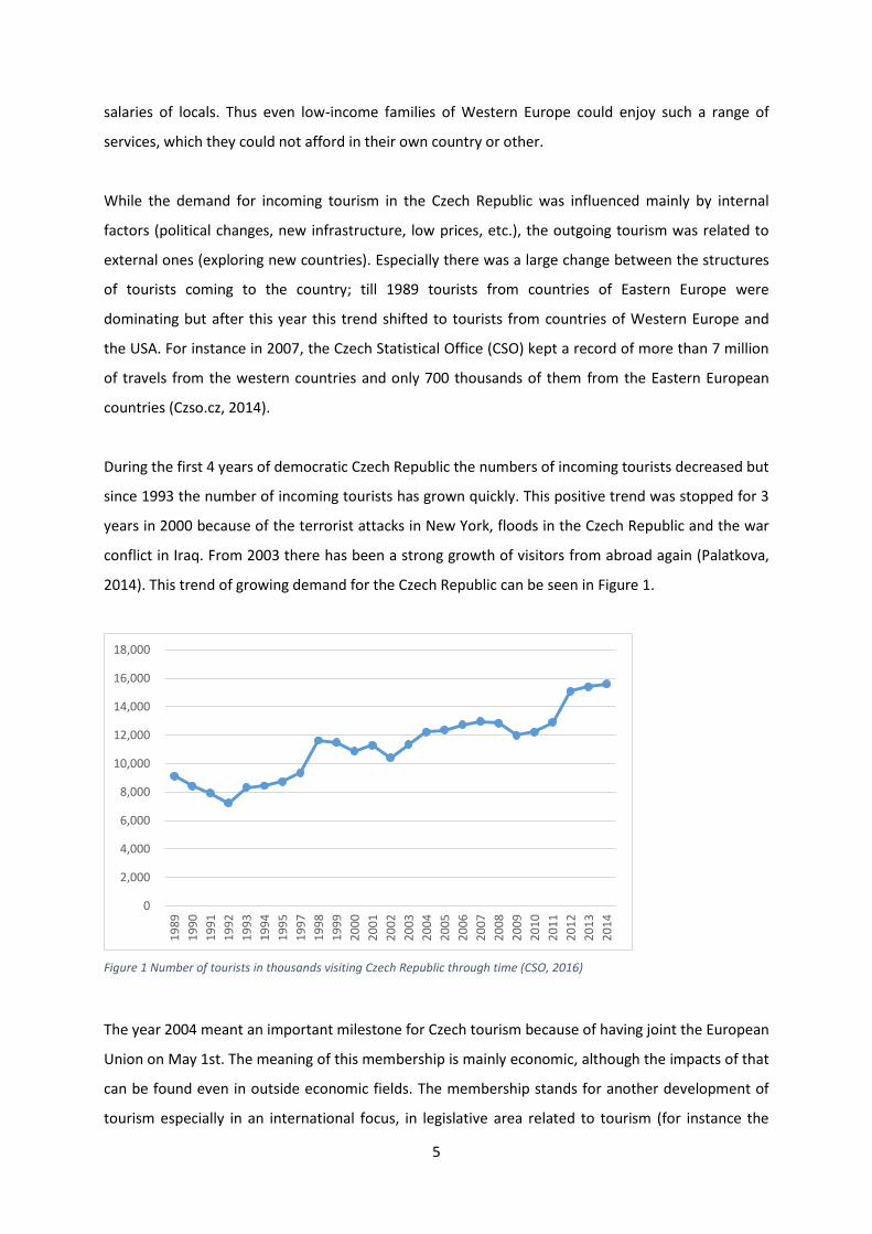
During the first 4 years of democratic Czech Republic the numbers of incoming tourists decreased but
since 1993 the number of incoming tourists has grown quickly. This positive trend was stopped for 3
years in 2000 because of the terrorist attacks in New York, floods in the Czech Republic and the war
conflict in Iraq. From 2003 there has been a strong growth of visitors from abroad again (Palatkova,
2014). This trend of growing demand for the Czech Republic can be seen in Figure 1.
Figure 1 Number of tourists in thousands visiting Czech Republic through time (CSO, 2016)
The year 2004 meant an important milestone for Czech tourism because of having joint the European
Union on May 1st. The meaning of this membership is mainly economic, although the impacts of that
can be found even in outside economic fields. The membership stands for another development of
tourism especially in an international focus, in legislative area related to tourism (for instance the
0
2,000
4,000
6,000
8,000
10,000
12,000
14,000
16,000
18,000
19
89
19
90
19
91
19
92
19
93
19
94
19
95
19
97
19
98
19
99
20
00
20
01
20
02
20
03
20
04
20
05
20
06
20
07
20
08
20
09
20
10
20
11
20
12
20
13
20
14
6
protection of consumers) and of course in the chance to gain financial support for tourism domestic
development. Another milestone connected to the membership of the European Union is that the
Czech Republic became a part of Schengen area on 21 December, 2007, which meant the
cancellation of border controls with the neighbor countries, that made travelling more simple.
The growing trend lasted till 2009 when the world financial crises resulted into a decrease of tourism
demand for the Czech Republic. This negative trend took place for only one year because already in
2010 there was a recovery of economy as well as in the growing number of visitors.
2.3 The structure of tourism demand in the Czech Republic
The tourism demand in the Czech Republic has been followed by statistics of the Czech Statistical
Office on arrivals that are accommodated in individual establishments (Czso.cz)).The number of
visitors and the amount of money they spend grows almost every year except from 2009 when
Europe was facing the financial crises (Ryglova, Burian, 2011).
Tourists from neighbor countries generate the largest share in the total amount of tourists. The
purposes of their visits are mostly the traditional forms of tourism (vacation or recreation - 65%), but
partially this number is influenced by people coming for shopping or business – 15 %. The second
largest group are Czechs that travel within the country but only 25% look for an accommodation and
the rest sleep in private establishments or at their relatives´ homes. That is the fundamental
difference between Czech visitors and the international visitors that are accommodated for 75% in
official establishments (CSO, 2016).
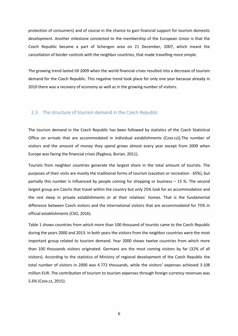
Table 1 shows countries from which more than 100 thousand of tourists came to the Czech Republic
during the years 2000 and 2013. In both years the visitors from the neighbor countries were the most
important group related to tourism demand. Year 2000 shows twelve countries from which more
than 100 thousands visitors originated. Germans are the most coming visitors by far (32% of all
visitors). According to the statistics of Ministry of regional development of the Czech Republic the
total number of visitors in 2000 was 4 772 thousands, while the visitors’ expenses achieved 3 108
million EUR. The contribution of tourism to tourism expenses through foreign currency revenues was
5.6% (Czso.cz, 2015).
7
Table 1 The structure of tourism demand in the Czech Republic in the years 2000 and 2013 (CSO, 2016)
Ranking In 2000 Total % In 2013 Total %
1. Germany 1 508 068 32% Germany 1 385 398 19%
2. Poland 332 933 7% Russia 759 138 10%
3. Netherlands 314 153 7% Slovak Republic 395 352 5%
4. United Kingdom 236 517 5% Poland 386 739 5%
5. Italy 233 179 5% USA 386 591 5%
6. USA 215 832 5% United Kingdom 353 973 5%
7. Israel 185 300 4% Italy 333 828 5%
8. France 161 782 3% France 270 798 4%
9. Slovak Republic 145 100 3% Austria 212 198 3%
10. Austria 137 743 3% Netherlands 185 464 3%
11. Spain 132 007 3% Spain 176 875 2%
12. Russia 103 077 2% China 163 857 2%
13. Republic of Korea 149 804 2%
14. Japan 130 740 2%
Year 2013 shows three additional countries – Republic of Korea, Japan and China– from which more
than 100 thousands of visitors originated. The reason is that the Czech Republic has become an
attractive destination for Asian countries. Total number of visitors was 7 309 thousands which means
53% growth of tourists during 12 years. The income from tourism to the Czech economy increased as
well by 61% to 5 010 million EUR (CSO, 2016). The relative proportion of German visitors reduced to
19% although in absolute figures this group still reflected the largest group of foreign visitors.
In 2014 about 17% of all accommodated tourists were Germans and the average number of days
they stayed was 4.1. The average expenses of average German tourists were about 1608 CZK a day
(60 EUR). 56% of the expenses were due to shopping, 29% for the fuel and 5% for food.
The characteristics of typical German tourists visiting the Czech Republic are obtained by statistics of
the Czech tourism (CSO, 2014). According to them Germans belong to a group called “Pleasure
Seekers”. It means that most of them present middle or higher aged tourists who seek for luxury
services related to passive relaxation. The Germans priorities are non - problematic travel, safety,
knowing foreign languages, large scale of spas and wellness, high quality of gastronomy etc. The trip
should be arranged and organized by travel agencies as a package of services. Travelers from this
segment of tourists are keen on travelling especially during weekends. Reasons of visiting the Czech
Republic are mainly related to long history and traditions, beautiful and diverse countryside, cultural
events and sights and by traffic availability and keenly priced goods and services (Czechtourism.cz,
2016).

8
9
3 Materials and Methods
3.1 Theoretical framework
Most of the models for tourism demand are based on the theory of consumer behavior that the
consumption depends on consumer´s income, the price of goods, the prices of related goods and
other factors. According to Matias and Nijkamp (2009) and Crouch (1994) income, relative prices,
transportation costs and exchange rates are the most used explanatory variables for estimating the
tourism demand.
Tourism demand analyses before 1990s were based on a regression approach. These regression
models used to have limited diagnostic tests and had a static form. Although they showed high R2
and a relationship between endogenous and exogenous variables, the standard regression analysis
failed when dealing with non-stationary variables, leading to spurious regressions that suggested
relationships even when there are none (Chen, 2011).
In the mid-1990s new approaches as Autoregressive Distributed Lag Model (ADLM) and Error
Correction model (ECM) were introduced. These methods were helpful mainly because they helped
to deal with the spurious regression problem.
For solving this spurious problem Engle and Granger (1987) and Johansen (1988) procedures have
been proved as a useful method for testing the cointegration. The cointegration analysis is connected
with a Granger representation theorem which states that if a set of variables is integrated, then there
exists a valid error correction representation of the data (Engle and Granger, 1987). In this paper
Johansen´s multiple cointegration analysis has been used because unlike the Engle and Granger
methodology, this procedure enables to indicate the number of cointegrating vectors among the
evaluated variables. This methodology includes two steps to test the presence of non-stationary data
series followed by a test on cointegration among the variables. Given the presence of co-inegration
among the variables, an Error Correction model has been defined to capture the rate of adjustment
among variables to restore long-run equilibrium in response to short-term disturbances in the
demand for tourism.
Given the determined rate of adjustments two methods were subsequently applied to forecast the
development in the next ten quarters of German demand, focusing on impacts of each variable
separately. The first method is the Impulse Response function which shows the effects on the
tourism demand of shocks of each exogenous variable in the form of one standard deviation. As the
second forecast method a Forecast Error Variance Decomposition FEVD is selected. FEVD helps to
10
estimate how each variable contributes to other variables in the VAR or VECM model. The results
indicate how much of the forecast error variance is determined by shocks to the other variables.
3.2 Definition tourism demand
Tourism demand is defined in different ways: first as the quantity of the tourism products (the
amount of tourism goods and services) that the arrivals are willing to buy during a certain period of
time (Asemota and Bala, 2012) or second directly by the number of tourists visiting the selected
country per time unit (Song and Witt, 2000).
Although Song and Li (2008) indicate that most of the tourism demand analyses use annual data, in
our case we will consider quarterly tourist arrivals from Germany as the tourism product (tourism
demand) as registered in the statistics of Ministry of Regional development in the Czech Republic and
Czech statistical office. In many times annual data do not meet the requirements of tourism related
businesses and their decision and policy makers because they are more interested in shorter terms –
hence the preference for the use of quarterly data (Song and Witt, 2000).
Information on the quarterly tourist arrivals is derived from the number of registered people in
collective accommodation establishments as recorded by the Ministry. This information was
recorded on a monthly base but as information on explanatory variables (see below) were recorded
in quarterly data, the original monthly data is aggregated to quarterly data. Germans visiting the
Czech Republic only for one day are as such not included.
Generally, significant variables that influence tourism demand include: income of the consumers,
tourism prices in the destination, tourism prices in substitute destinations, expenditure on
advertising, tastes of the consumers in origin country and factors from social and geographical fields
(changes in weather or climate, socio-cultural relations between countries) to the political factors
(political relationships between countries, government regulation on supply and tourists, visas,
currency, prohibitions) (Song and Witt, 2000). Matias and Nijkamp (2009) and Crouch (1994)
indicated that among these variables tourist income, relative price differences, transportation costs
and exchange rates are the most used explanatory variables for estimating the tourism demand.
Due to a limitation in available data on tourism in Czech Republic, the model in this study will
account only for the main explanatory variables related to arrivals´ income, tourism prices adapted
by exchange rates and travelling costs.
11
Arrivals´ income
One of the most important explanatory variables is the arrivals´ income and it is usually expressed in
per capita form. If it is considered that the main reason for visiting the selected country is to meet
the relatives or friends then the personal disposable income or private consumption should be
included in the function. According to Song and Witt (2000) when it is assumed that people come to
the Czech Republic because of business reasons as well it is necessary to use more appropriate
general data as a variable of arrivals´ income – GDP per capita.
We will use quarterly GDP per capita as an arrivals´ income in tourism demand (Song and Witt, 2000).
Because the quarterly data GDP per capita were missing in the statistics, the time series was
calculated as German quarter GDP divided by the German population in the individual years. The
GDP per capita is expressed in millions of euros.
Tourism prices
In our case we will consider consumer price index as an appropriate measure of tourism prices in the
destined country. The issue with the Consumer Price Index - CPI is that the basket of goods bought by
tourists in the destined country is not always the same as the basket of locals and the biggest
difference can be found especially in poor countries. The tourists always recalculate the cost of good
in the foreign currency to their local currency so receiving the most exact and appropriate results the
basket of goods should be adjusted by the exchange rate (Song, Witt and Li, 2009). In our case CPI is
used as the cost of tourism in the Czech Republic relative to the cost of living in Germany.
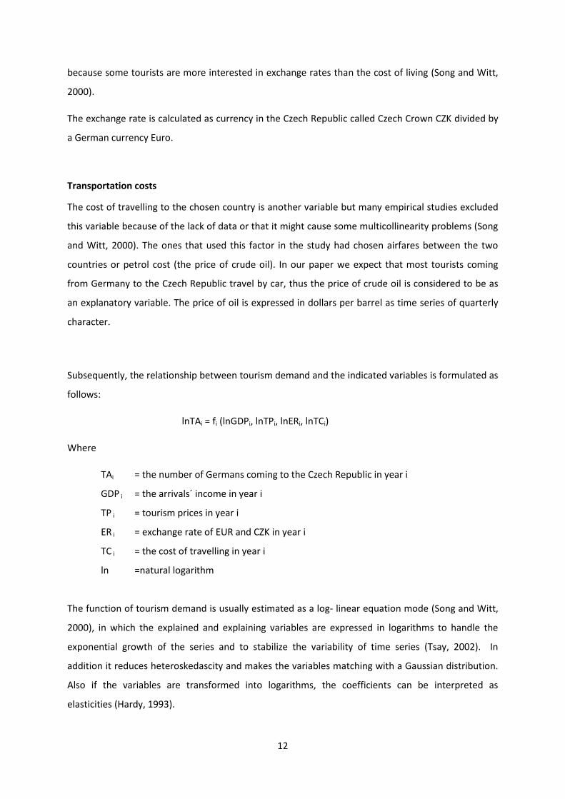
The own price time series are estimated by the following formula:
𝑇𝑃 =𝐶𝑃𝐼𝑐𝑧𝑒 𝑖
𝐶𝑃𝐼𝑔𝑒𝑟 𝑖
Where
TP = tourism prices
CPIczeI = consumer price index in the Czech Republic in year i
CPIGeri = consumer price index in the Germany in year i
The exchange rate
In many researches exchange rate is often used as another exogenous variable. In some of them it is
added to the consumer price index but in our research exchange rate stands as an individual variable
12
because some tourists are more interested in exchange rates than the cost of living (Song and Witt,
2000).
The exchange rate is calculated as currency in the Czech Republic called Czech Crown CZK divided by
a German currency Euro.
Transportation costs
The cost of travelling to the chosen country is another variable but many empirical studies excluded
this variable because of the lack of data or that it might cause some multicollinearity problems (Song
and Witt, 2000). The ones that used this factor in the study had chosen airfares between the two
countries or petrol cost (the price of crude oil). In our paper we expect that most tourists coming
from Germany to the Czech Republic travel by car, thus the price of crude oil is considered to be as
an explanatory variable. The price of oil is expressed in dollars per barrel as time series of quarterly
character.
Subsequently, the relationship between tourism demand and the indicated variables is formulated as
follows:
lnTAi = fi (lnGDPi, lnTPi, lnERi, lnTCi)
Where
TAi = the number of Germans coming to the Czech Republic in year i
GDP i = the arrivals´ income in year i
TP i = tourism prices in year i
ER i = exchange rate of EUR and CZK in year i
TC i = the cost of travelling in year i
ln =natural logarithm
The function of tourism demand is usually estimated as a log- linear equation mode (Song and Witt,
2000), in which the explained and explaining variables are expressed in logarithms to handle the
exponential growth of the series and to stabilize the variability of time series (Tsay, 2002). In
addition it reduces heteroskedascity and makes the variables matching with a Gaussian distribution.
Also if the variables are transformed into logarithms, the coefficients can be interpreted as
elasticities (Hardy, 1993).
13
3.3 Data
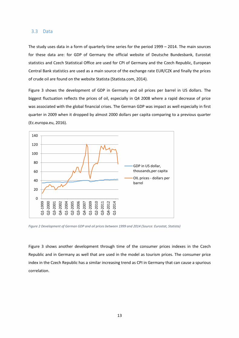
The study uses data in a form of quarterly time series for the period 1999 – 2014. The main sources
for these data are: for GDP of Germany the official website of Deutsche Bundesbank, Eurostat
statistics and Czech Statistical Office are used for CPI of Germany and the Czech Republic, European
Central Bank statistics are used as a main source of the exchange rate EUR/CZK and finally the prices
of crude oil are found on the website Statista (Statista.com, 2014).
Figure 3 shows the development of GDP in Germany and oil prices per barrel in US dollars. The
biggest fluctuation reflects the prices of oil, especially in Q4 2008 where a rapid decrease of price
was associated with the global financial crises. The German GDP was impact as well especially in first
quarter in 2009 when it dropped by almost 2000 dollars per capita comparing to a previous quarter
(Ec.europa.eu, 2016).
Figure 2 Development of German GDP and oil prices between 1999 and 2014 (Source: Eurostat, Statista)
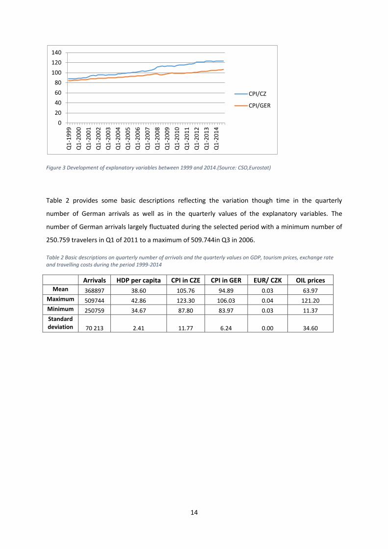
Figure 3 shows another development through time of the consumer prices indexes in the Czech
Republic and in Germany as well that are used in the model as tourism prices. The consumer price
index in the Czech Republic has a similar increasing trend as CPI in Germany that can cause a spurious
correlation.
0
20
40
60
80
100
120
140
Q1
-19
99
Q2
-20
00
Q3
-20
01
Q4
-20
02
Q1
-20
04
Q2
-20
05
Q3
-20
06
Q4
-20
07
Q1
-20
09
Q2
-20
10
Q3
-20
11
Q4
-20
12
Q1
-20
14
GDP in US dollar,thousands,per capita
OIL prices - dollars perbarrel
14
Figure 3 Development of explanatory variables between 1999 and 2014.(Source: CSO,Eurostat)
Table 2 provides some basic descriptions reflecting the variation though time in the quarterly
number of German arrivals as well as in the quarterly values of the explanatory variables. The
number of German arrivals largely fluctuated during the selected period with a minimum number of
250.759 travelers in Q1 of 2011 to a maximum of 509.744in Q3 in 2006.
Table 2 Basic descriptions on quarterly number of arrivals and the quarterly values on GDP, tourism prices, exchange rate and travelling costs during the period 1999-2014
Arrivals HDP per capita CPI in CZE CPI in GER EUR/ CZK OIL prices
Mean 368897 38.60 105.76 94.89 0.03 63.97
Maximum 509744 42.86 123.30 106.03 0.04 121.20
Minimum 250759 34.67 87.80 83.97 0.03 11.37
Standard deviation 70 213 2.41 11.77 6.24 0.00 34.60
0
20
40
60
80
100
120
140
Q1
-19
99
Q1
-20
00
Q1
-20
01
Q1
-20
02
Q1
-20
03
Q1
-20
04
Q1
-20
05
Q1
-20
06
Q1
-20
07
Q1
-20
08
Q1
-20
09
Q1
-20
10
Q1
-20
11
Q1
-20
12
Q1
-20
13
Q1
-20
14
CPI/CZ
CPI/GER
15
3.4 Methods
Performed Cointegration analysis
- Augmented Dickey Fuller test to test the order of integration
Data are often non-stationary having means, variances and covariances that change over time. A
non-stationary time series is known as a series that has unit roots. The number of unit roots is equal
to the number of times the series must be differenced in order to gain stationary series. If the time
series becomes stationary after first difference, then yt has one unit root I(1) or so called is integrated
in one order.
Assume that we have a time series {𝑦𝑡} 𝑇𝑡=1
that is generated by simple AR(1) process:
Yt = a1 𝑦𝑡−1 + 𝜀𝑡
Where 𝜀𝑡 are independent normal disturbances with zero mean and variance σ2. This simple case is
stationary if |𝑎1|<1 and it contains a unit root if |𝑎1|=1. But in economic time series it happens only
rarely that a1 would be negative (Kocenda et al., 2015).
One of the test that can be used for testing unit root is Augmented Dickey-Fuller (ADF). The ADF test
is done by this model:
∆𝑦𝑡 = γ𝑦𝑡−1 + ∑ 𝛽𝑖∆𝑦𝑡−𝑖+1
𝑝
𝑖=1
+ 𝜀𝑡
Where ∆𝑦𝑡 expresses the lagged first difference
p are the lags of ∆𝑦𝑡,
𝛽, γ are the parameters to be estimated,
γ = ∑ a𝑝𝑖=1 i-1 and βi =− ∑ a
𝑝𝑗=1 j
This augmented specification is tested for the following hypothesis in the above regression
(Middleton, 1995).
H0: γ = 0 of a unit root time series
Against the alternative
Ha: γ< 0 of a stationary time series
If the coefficient γ=0, then ∑ a𝑝𝑖=1 I =1. Similarly if γ <0, then ∑ a
𝑝𝑖=1 i<1.
16
To test the null hypothesis which says that the data is non stationary we calculate DF t statistics. By
including lagged differences in the estimated equation, the model is corrected for possible
autocorrelation in the residuals, thus it is necessary to choose an appropriate lag length for the
dependent variable. The reason for it is that the power of the test decreases with more lags used to
correct the autocorrelation of residuals (Kocenda et al., 2015). The lag length can be chosen by many
criterias: R2, the Akaike information criterion (AIC) or Schwarz info criterion (SIC) (Song and Witt,
2000). It is recommended to use the initial lag length four because we use quarterly data in the
model (Brooks, 2002). These four lags are tested and where the fourth lag is insignificant, the
number of lags is reduced until it reaches a significance. If no lagged first differences are used, the
ADF test is reduced to standard Dickey-fuller test (Dritsakis, 2004). In this study the ADF test is used
for each time series variable in the model.
- The Johansen procedure
When the hypothesis of a unit root is not rejected - meaning data are non-stationary - then it is
possible to run a cointegration test. Although the time series variables are non-stationary, in their
levels they can be integrated (of order one) which means that their first differences are stationary. If
there is cointegration among the variables, then there is a stable long run or equilibrium linear
relationship among them. Johansen (1988) proposed a methodology that investigates the
cointegration with a larger complexity than Engle-Granger methodology. It enables to test the
number of cointegrating vectors among N variables. Johansen´s approach is derived from the error
correction model that is described underneath:
∆Yt = µ+ Π Yt-1 + ∑ Π𝑖∆𝑝𝑖=1 Yt-i +𝜀𝑡
Where yt=(y1t,y2t,…yNt) is N x 1 vector of the N cointegrated variables
𝜀𝑡=(𝜀1, 𝜀2…𝜀𝑁𝑡) is N x 1 vector of N possible correlated white noise disturbances
µ=( µ1, µ2,… µN) is N x 1 vector of intercepts
Πi are N x N matrixes of autoregressive coefficients
Π = 𝛼𝛽′ is N x N matrix that is by construction r ≤ N-1, thus the rank of the matrix is equal to the
cointegrating rank r
β = (β1, β2,…, βr) is the N x r cointegrating matrix consisting of the r cointegrating vectors
𝛼 is N x r matrix of the r adjustment coefficients for each of the N variables (Kocenda et al., 2015)
17
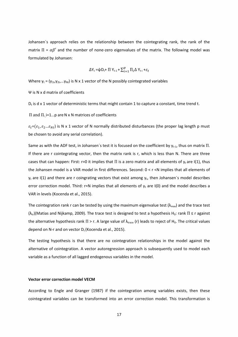
Johansen´s approach relies on the relationship between the cointegrating rank, the rank of the
matrix Π = 𝛼𝛽′ and the number of none-zero eigenvalues of the matrix. The following model was
formulated by Johansen:
∆Yt =ψDt+ Π Yt-1 + ∑ Π𝑖∆𝑝𝑖=1 Yt-i +𝜀𝑡
Where yt = (y1t,y2t,…yNt) is N x 1 vector of the N possibly cointegrated variables
Ψ is N x d matrix of coefficients
Dt is d x 1 vector of deterministic terms that might contain 1 to capture a constant, time trend t.
Π and Πi ,i=1…p are N x N matrices of coefficients
𝜀𝑡=(𝜀1, 𝜀2…𝜀𝑁𝑡) is N x 1 vector of N normally distributed disturbances (the proper lag length p must
be chosen to avoid any serial correlation).
Same as with the ADF test, in Johansen´s test it is focused on the coefficient by yt-1, thus on matrix Π.
If there are r cointegrating vector, then the matrix rank is r, which is less than N. There are three
cases that can happen: First: r=0 it implies that Π is a zero matrix and all elements of yt are I(1), thus
the Johansen model is a VAR model in first differences. Second: 0 < r <N implies that all elements of
yt are I(1) and there are r coingrating vectors that exist among yt, then Johansen´s model describes
error correction model. Third: r=N implies that all elements of yt are I(0) and the model describes a
VAR in levels (Kocenda et al., 2015).
The cointegration rank r can be tested by using the maximum eigenvalue test (λmax) and the trace test
(λtr)(Matias and Nijkamp, 2009). The trace test is designed to test a hypothesis H0: rank Π ≤ r against
the alternative hypothesis rank Π > r. A large value of λtrace (r) leads to reject of H0. The critical values
depend on N-r and on vector Dt (Kocenda et al., 2015).
The testing hypothesis is that there are no cointegration relationships in the model against the
alternative of cointegration. A vector autoregression approach is subsequently used to model each
variable as a function of all lagged endogenous variables in the model.
Vector error correction model VECM
According to Engle and Granger (1987) if the cointegration among variables exists, then these
cointegrated variables can be transformed into an error correction model. This transformation is
18
known as Granger Representation Theorem which indicates that there is some process that prevents
the selected variables to move away from their long-run equilibrium. The method of cointegration
and error correction model helps to estimate the short-run and long-run equilibrium and it will
examine if the variables have a positive or negative relationship to the tourism demand yt.
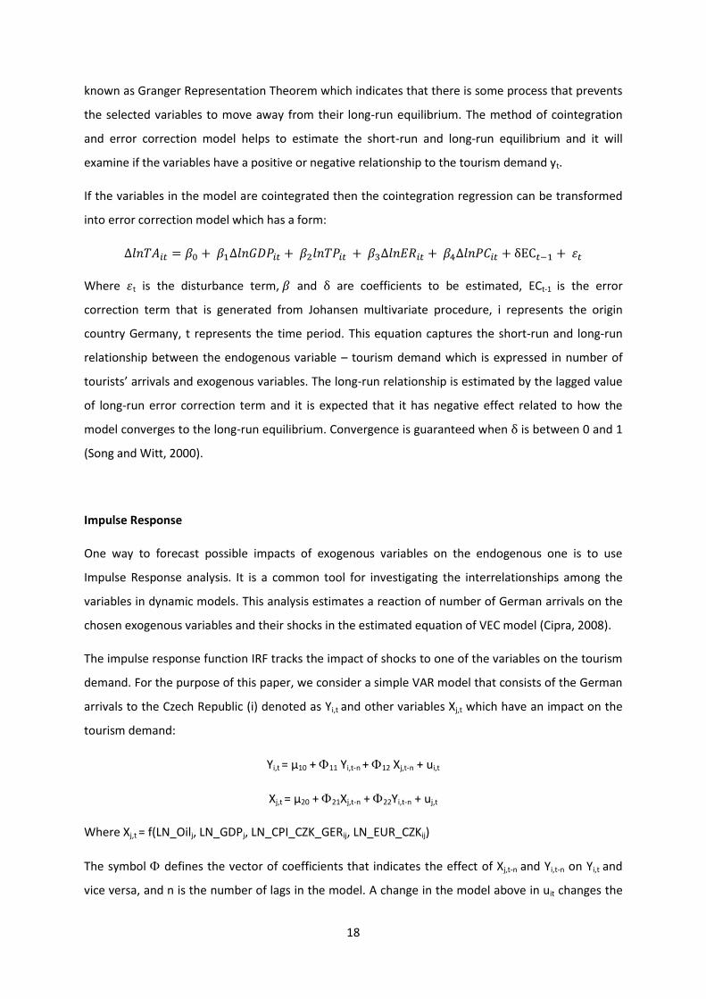
If the variables in the model are cointegrated then the cointegration regression can be transformed
into error correction model which has a form:
∆𝑙𝑛𝑇𝐴𝑖𝑡 = 𝛽0 + 𝛽1∆𝑙𝑛𝐺𝐷𝑃𝑖𝑡 + 𝛽2𝑙𝑛𝑇𝑃𝑖𝑡 + 𝛽3∆𝑙𝑛𝐸𝑅𝑖𝑡 + 𝛽4∆𝑙𝑛𝑃𝐶𝑖𝑡 + δEC𝑡−1 + 𝜀𝑡
Where 𝜀t is the disturbance term, 𝛽 and δ are coefficients to be estimated, ECt-1 is the error
correction term that is generated from Johansen multivariate procedure, i represents the origin
country Germany, t represents the time period. This equation captures the short-run and long-run
relationship between the endogenous variable – tourism demand which is expressed in number of
tourists’ arrivals and exogenous variables. The long-run relationship is estimated by the lagged value
of long-run error correction term and it is expected that it has negative effect related to how the
model converges to the long-run equilibrium. Convergence is guaranteed when δ is between 0 and 1
(Song and Witt, 2000).
Impulse Response
One way to forecast possible impacts of exogenous variables on the endogenous one is to use
Impulse Response analysis. It is a common tool for investigating the interrelationships among the
variables in dynamic models. This analysis estimates a reaction of number of German arrivals on the
chosen exogenous variables and their shocks in the estimated equation of VEC model (Cipra, 2008).
The impulse response function IRF tracks the impact of shocks to one of the variables on the tourism
demand. For the purpose of this paper, we consider a simple VAR model that consists of the German
arrivals to the Czech Republic (i) denoted as Yi,t and other variables Xj,t which have an impact on the
tourism demand:
Yi,t = μ10 + 11 Yi,t-n + 12 Xj,t-n + ui,t
Xj,t = μ20 + 21Xj,t-n + 22Yi,t-n + uj,t
Where Xj,t = f(LN_Oilj, LN_GDPj, LN_CPI_CZK_GERij, LN_EUR_CZKij)
The symbol defines the vector of coefficients that indicates the effect of Xj,t-n and Yi,t-n on Yi,t and
vice versa, and n is the number of lags in the model. A change in the model above in uit changes the

19
future values of Y and X because lagged Y is in both equations. If it is assumed that uit and ujt are not
correlated, then IRF reflects that the innovation of uit has an impact on Y and uij effects X
(Gaunoploulos et al, 2012).
Because the changes of uit and ujt are most of the time correlated, it means that they contain a
common part that cannot be equated with a specific variable. To deal with such an issue it is
common to impute the whole impact of any common component to the variable that comes to the
system as the first. In our equations the common part of uit and ujt is uit meaning that the changes of
uit come before ujt. Thus uit innovates Y and X, that are transformed to remove the common
component. Using the Cholesky decomposition the innovations are transformed by orthogonalising
the errors. The vector of orthogonal innovations is defined as et
E ( ei,t, ej,t) = 0 where I ≠ j
A (N x N) lower matrix defined as V is used to transform error terms and the et are obtained from
following (Gaunoploulos et al, 2012):
e= uV-1
Where ut means a covariance matrix
EeeT =
And
VVT =
Then the model can be estimated as
Yt = ∑ 𝐵∞𝑛=0 net-n
Where Bn=AnV.
Bn at the formula above represents the effects of impulse response of the tourism demand in the
future to one positive standard deviation shock in time t (Gaunoploulos et al, 2012).
Forecast Error Variance Decomposition
While Impulse Response catches the influence of impulse of independent variables on the selected
dependent variable, Variance Decomposition provides information of relative influence of
innovations from the individual equations on the selected variable (Cipra, 2008).
20
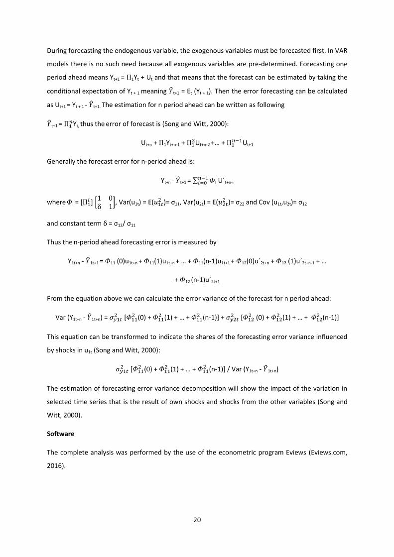
During forecasting the endogenous variable, the exogenous variables must be forecasted first. In VAR
models there is no such need because all exogenous variables are pre-determined. Forecasting one
period ahead means Yt+1 = Π1Yt + Ut and that means that the forecast can be estimated by taking the
conditional expectation of Yt + 1 meaning ��t+1 = Et (Yt + 1). Then the error forecasting can be calculated
as Ut+1 = Yt + 1 - ��t+1. The estimation for n period ahead can be written as following
��t+1 = Π1𝑛Yt, thus the error of forecast is (Song and Witt, 2000):
Ut+n + Π1Yt+n-1 + Π12Ut+n-2 +… + Π1
𝑛−1Ut+1
Generally the forecast error for n-period ahead is:
Yt+n - ��t+1 = ∑ 𝛷𝑛−1𝑖=0 I U´t+n-i
where 𝛷i = [Π1𝑖 ] [
1 0δ 1
], Var(u1t) = E(𝑢1𝑡2 )= σ11, Var(u2t) = E(𝑢2𝑡
2 )= σ22 and Cov (u1t,u2t)= σ12
and constant term δ = σ12/ σ11
Thus the n-period ahead forecasting error is measured by
Y1t+n - ��1t+1 = 𝛷11 (0)u1t+n + 𝛷11(1)u1t+n + … + 𝛷11(n-1)u1t+1 + 𝛷12(0)u´2t+n + 𝛷12 (1)u´2t+n-1 + …
+ 𝛷12 (n-1)u´2t+1
From the equation above we can calculate the error variance of the forecast for n period ahead:
Var (Y1t+n - ��1t+n) = 𝜎𝑦1𝑡2 [𝛷11
2 (0) + 𝛷112 (1) + … + 𝛷11
2 (n-1)] + 𝜎𝑦2𝑡2 [𝛷12
2 (0) + 𝛷122 (1) + … + 𝛷12
2 (n-1)]
This equation can be transformed to indicate the shares of the forecasting error variance influenced
by shocks in u1t (Song and Witt, 2000):
𝜎𝑦1𝑡2 [𝛷11
2 (0) + 𝛷112 (1) + … + 𝛷11
2 (n-1)] / Var (Y1t+n - ��1t+n)
The estimation of forecasting error variance decomposition will show the impact of the variation in
selected time series that is the result of own shocks and shocks from the other variables (Song and
Witt, 2000).
Software
The complete analysis was performed by the use of the econometric program Eviews (Eviews.com,
2016).
21
4 Results
4.1 Cointegration analysis
Augmented Dickey Fuller test
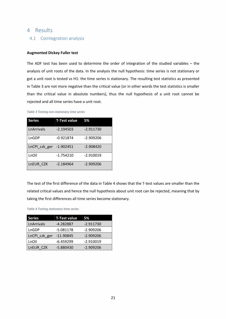
The ADF test has been used to determine the order of integration of the studied variables – the
analysis of unit roots of the data. In the analysis the null hypothesis: time series is not stationary or
got a unit root is tested vs H1: the time series is stationary. The resulting test statistics as presented
in Table 3 are not more negative than the critical value (or in other words the test statistics is smaller
than the critical value in absolute numbers), thus the null hypothesis of a unit root cannot be
rejected and all time series have a unit root.
Table 3 Testing non-stationary time series
Series T-Test value 5%
LnArrivals -2.194503 -2.911730
LnGDP -0.921874 -2.909206
LnCPI_czk_ger -1.902451 -2.908420
LnOil -1.754210 -2.910019
LnEUR_CZK -2.184964 -2.909206
The test of the first difference of the data in Table 4 shows that the T-test values are smaller than the
related critical values and hence the null hypothesis about unit root can be rejected, meaning that by
taking the first differences all time series become stationary.
Table 4 Testing stationary time-series
Series T-Test value 5%
LnArrivals -4.282887 -2.911730
LnGDP -5.081178 -2.909206
LnCPI_czk_ger -11.90845 -2.909206
LnOil -6.459299 -2.910019
LnEUR_CZK -5.880430 -2.909206
22
Cointegration analysis:
As all time series have a unit root, in other words they are non-stationary I (1), the following step is
to test the time series for cointegrative relationships between the variables LnArrivals, LnGDP,
LnCPI_czk_ger , Ln_EUR_CZK and LnOil by the Johansen approach.
The first hypothesis that is tested is: there is no cointegration between variables.
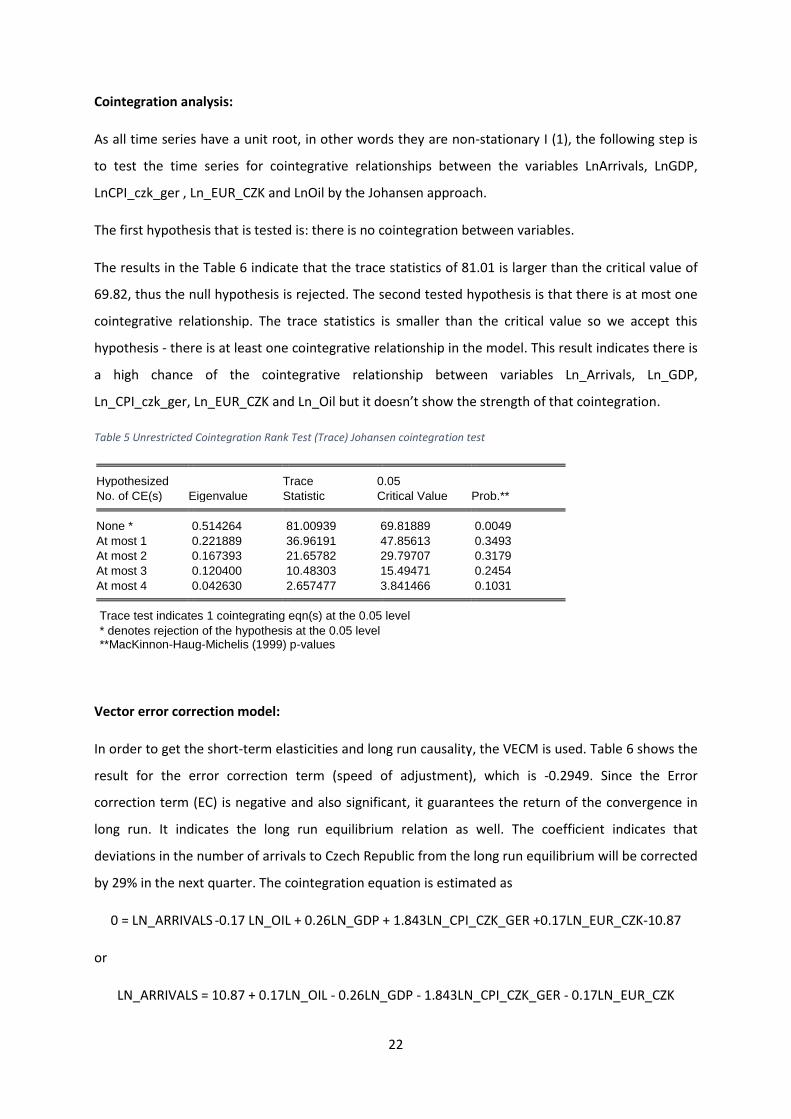
The results in the Table 6 indicate that the trace statistics of 81.01 is larger than the critical value of
69.82, thus the null hypothesis is rejected. The second tested hypothesis is that there is at most one
cointegrative relationship. The trace statistics is smaller than the critical value so we accept this
hypothesis - there is at least one cointegrative relationship in the model. This result indicates there is
a high chance of the cointegrative relationship between variables Ln_Arrivals, Ln_GDP,
Ln_CPI_czk_ger, Ln_EUR_CZK and Ln_Oil but it doesn’t show the strength of that cointegration.
Table 5 Unrestricted Cointegration Rank Test (Trace) Johansen cointegration test
Hypothesized Trace 0.05
No. of CE(s) Eigenvalue Statistic Critical Value Prob.** None * 0.514264 81.00939 69.81889 0.0049
At most 1 0.221889 36.96191 47.85613 0.3493
At most 2 0.167393 21.65782 29.79707 0.3179
At most 3 0.120400 10.48303 15.49471 0.2454
At most 4 0.042630 2.657477 3.841466 0.1031 Trace test indicates 1 cointegrating eqn(s) at the 0.05 level
* denotes rejection of the hypothesis at the 0.05 level **MacKinnon-Haug-Michelis (1999) p-values
Vector error correction model:
In order to get the short-term elasticities and long run causality, the VECM is used. Table 6 shows the
result for the error correction term (speed of adjustment), which is -0.2949. Since the Error
correction term (EC) is negative and also significant, it guarantees the return of the convergence in
long run. It indicates the long run equilibrium relation as well. The coefficient indicates that
deviations in the number of arrivals to Czech Republic from the long run equilibrium will be corrected
by 29% in the next quarter. The cointegration equation is estimated as
0 = LN_ARRIVALS -0.17 LN_OIL + 0.26LN_GDP + 1.843LN_CPI_CZK_GER +0.17LN_EUR_CZK-10.87
or
LN_ARRIVALS = 10.87 + 0.17LN_OIL - 0.26LN_GDP - 1.843LN_CPI_CZK_GER - 0.17LN_EUR_CZK
23
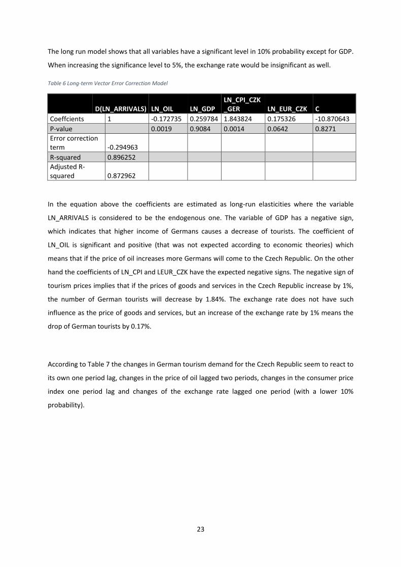
The long run model shows that all variables have a significant level in 10% probability except for GDP.
When increasing the significance level to 5%, the exchange rate would be insignificant as well.
Table 6 Long-term Vector Error Correction Model
D(LN_ARRIVALS) LN_OIL LN_GDP
LN_CPI_CZK_GER LN_EUR_CZK C
Coeffcients 1 -0.172735 0.259784 1.843824 0.175326 -10.870643
P-value 0.0019 0.9084 0.0014 0.0642 0.8271
Error correction term -0.294963
R-squared 0.896252
Adjusted R-squared 0.872962
In the equation above the coefficients are estimated as long-run elasticities where the variable
LN_ARRIVALS is considered to be the endogenous one. The variable of GDP has a negative sign,
which indicates that higher income of Germans causes a decrease of tourists. The coefficient of
LN_OIL is significant and positive (that was not expected according to economic theories) which
means that if the price of oil increases more Germans will come to the Czech Republic. On the other
hand the coefficients of LN_CPI and LEUR_CZK have the expected negative signs. The negative sign of
tourism prices implies that if the prices of goods and services in the Czech Republic increase by 1%,
the number of German tourists will decrease by 1.84%. The exchange rate does not have such
influence as the price of goods and services, but an increase of the exchange rate by 1% means the
drop of German tourists by 0.17%.
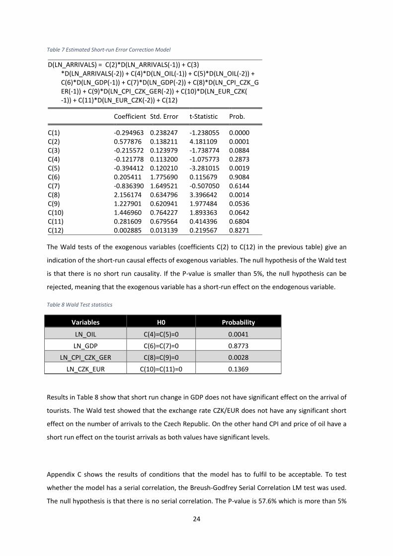
According to Table 7 the changes in German tourism demand for the Czech Republic seem to react to
its own one period lag, changes in the price of oil lagged two periods, changes in the consumer price
index one period lag and changes of the exchange rate lagged one period (with a lower 10%
probability).
24
Table 7 Estimated Short-run Error Correction Model
D(LN_ARRIVALS) = C(2)*D(LN_ARRIVALS(-1)) + C(3) *D(LN_ARRIVALS(-2)) + C(4)*D(LN_OIL(-1)) + C(5)*D(LN_OIL(-2)) + C(6)*D(LN_GDP(-1)) + C(7)*D(LN_GDP(-2)) + C(8)*D(LN_CPI_CZK_G ER(-1)) + C(9)*D(LN_CPI_CZK_GER(-2)) + C(10)*D(LN_EUR_CZK( -1)) + C(11)*D(LN_EUR_CZK(-2)) + C(12) Coefficient Std. Error t-Statistic Prob. C(1) -0.294963 0.238247 -1.238055 0.0000 C(2) 0.577876 0.138211 4.181109 0.0001 C(3) -0.215572 0.123979 -1.738774 0.0884 C(4) -0.121778 0.113200 -1.075773 0.2873 C(5) -0.394412 0.120210 -3.281015 0.0019 C(6) 0.205411 1.775690 0.115679 0.9084 C(7) -0.836390 1.649521 -0.507050 0.6144 C(8) 2.156174 0.634796 3.396642 0.0014 C(9) 1.227901 0.620941 1.977484 0.0536 C(10) 1.446960 0.764227 1.893363 0.0642 C(11) 0.281609 0.679564 0.414396 0.6804 C(12) 0.002885 0.013139 0.219567 0.8271
The Wald tests of the exogenous variables (coefficients C(2) to C(12) in the previous table) give an
indication of the short-run causal effects of exogenous variables. The null hypothesis of the Wald test
is that there is no short run causality. If the P-value is smaller than 5%, the null hypothesis can be
rejected, meaning that the exogenous variable has a short-run effect on the endogenous variable.
Table 8 Wald Test statistics
Variables H0 Probability
LN_OIL C(4)=C(5)=0 0.0041
LN_GDP C(6)=C(7)=0 0.8773
LN_CPI_CZK_GER C(8)=C(9)=0 0.0028
LN_CZK_EUR C(10)=C(11)=0 0.1369
Results in Table 8 show that short run change in GDP does not have significant effect on the arrival of
tourists. The Wald test showed that the exchange rate CZK/EUR does not have any significant short
effect on the number of arrivals to the Czech Republic. On the other hand CPI and price of oil have a
short run effect on the tourist arrivals as both values have significant levels.
Appendix C shows the results of conditions that the model has to fulfil to be acceptable. To test
whether the model has a serial correlation, the Breush-Godfrey Serial Correlation LM test was used.
The null hypothesis is that there is no serial correlation. The P-value is 57.6% which is more than 5%
25
meaning that we accept the null hypothesis, thus the data are non-correlated. To test
heteroscedasticity we used the Breusch-Pagan-Godfrey test where null hypothesis means that model
is homoscedastic. The null hypothesis is accepted when the P-value is larger than 5%. Our model
showed P-value as 43.27%, thus the model is homoscedastic. To test normality the Jargue-Bera
statistic and its P-value was used. The null hypothesis is that the residuals are normally distributed.
The P-value is 77.5% which means that we cannot reject the null hypothesis and residuals are
normally distributed. This model has carried out all the requirements and conditions, R squared is
89% that indicates that our model has a large explanatory value.
4.2 Impulse Response and Forecast error variance decomposition
IMPULSE RESPONSE FUNCTIONS
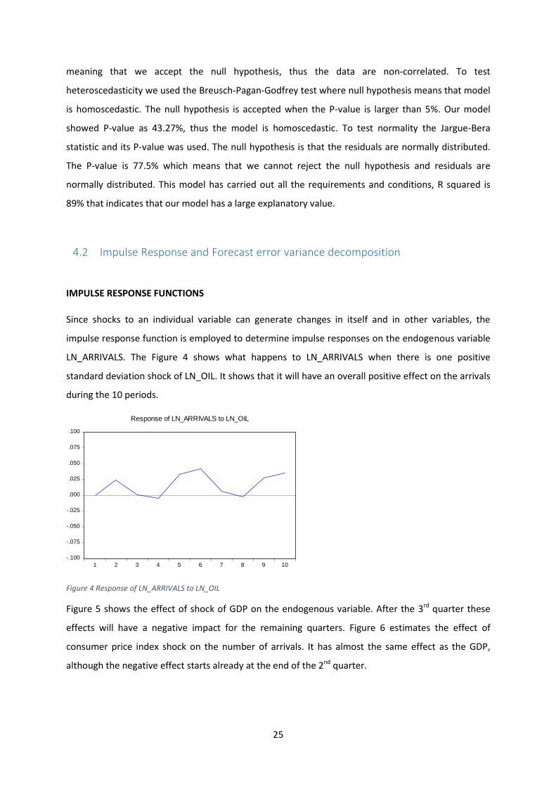
Since shocks to an individual variable can generate changes in itself and in other variables, the
impulse response function is employed to determine impulse responses on the endogenous variable
LN_ARRIVALS. The Figure 4 shows what happens to LN_ARRIVALS when there is one positive
standard deviation shock of LN_OIL. It shows that it will have an overall positive effect on the arrivals
during the 10 periods.
Figure 4 Response of LN_ARRIVALS to LN_OIL
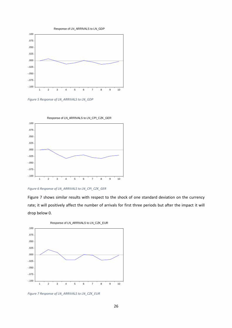
Figure 5 shows the effect of shock of GDP on the endogenous variable. After the 3rd quarter these
effects will have a negative impact for the remaining quarters. Figure 6 estimates the effect of
consumer price index shock on the number of arrivals. It has almost the same effect as the GDP,
although the negative effect starts already at the end of the 2nd quarter.
-.100
-.075
-.050
-.025
.000
.025
.050
.075
.100
1 2 3 4 5 6 7 8 9 10
Response of LN_ARRIVALS to LN_OIL
26
Figure 5 Response of LN_ARRIVALS to LN_GDP
Figure 6 Response of LN_ARRIVALS to LN_CPI_CZK_GER
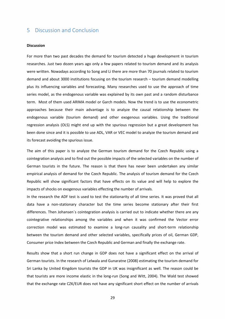
Figure 7 shows similar results with respect to the shock of one standard deviation on the currency
rate; it will positively affect the number of arrivals for first three periods but after the impact it will
drop below 0.
Figure 7 Response of LN_ARRIVALS to LN_CZK_EUR
-.100
-.075
-.050
-.025
.000
.025
.050
.075
.100
1 2 3 4 5 6 7 8 9 10
Response of LN_ARRIVALS to LN_GDP
-.100
-.075
-.050
-.025
.000
.025
.050
.075
.100
1 2 3 4 5 6 7 8 9 10
Response of LN_ARRIVALS to LN_CPI_CZK_GER
-.100
-.075
-.050
-.025
.000
.025
.050
.075
.100
1 2 3 4 5 6 7 8 9 10
Response of LN_ARRIVALS to LN_CZK_EUR
27
4.3 Forecast error variance decomposition
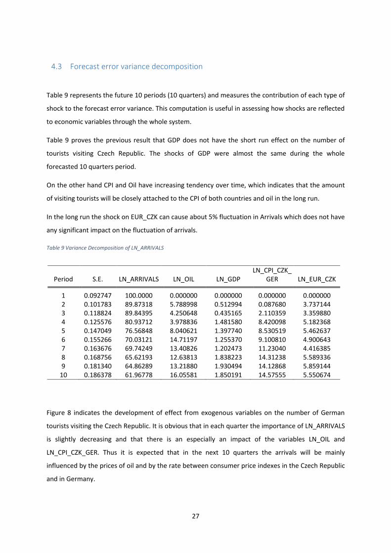
Table 9 represents the future 10 periods (10 quarters) and measures the contribution of each type of
shock to the forecast error variance. This computation is useful in assessing how shocks are reflected
to economic variables through the whole system.
Table 9 proves the previous result that GDP does not have the short run effect on the number of
tourists visiting Czech Republic. The shocks of GDP were almost the same during the whole
forecasted 10 quarters period.
On the other hand CPI and Oil have increasing tendency over time, which indicates that the amount
of visiting tourists will be closely attached to the CPI of both countries and oil in the long run.
In the long run the shock on EUR_CZK can cause about 5% fluctuation in Arrivals which does not have
any significant impact on the fluctuation of arrivals.
Table 9 Variance Decomposition of LN_ARRIVALS
Period S.E. LN_ARRIVALS LN_OIL LN_GDP LN_CPI_CZK_
GER LN_EUR_CZK 1 0.092747 100.0000 0.000000 0.000000 0.000000 0.000000
2 0.101783 89.87318 5.788998 0.512994 0.087680 3.737144 3 0.118824 89.84395 4.250648 0.435165 2.110359 3.359880 4 0.125576 80.93712 3.978836 1.481580 8.420098 5.182368 5 0.147049 76.56848 8.040621 1.397740 8.530519 5.462637 6 0.155266 70.03121 14.71197 1.255370 9.100810 4.900643 7 0.163676 69.74249 13.40826 1.202473 11.23040 4.416385 8 0.168756 65.62193 12.63813 1.838223 14.31238 5.589336 9 0.181340 64.86289 13.21880 1.930494 14.12868 5.859144
10 0.186378 61.96778 16.05581 1.850191 14.57555 5.550674
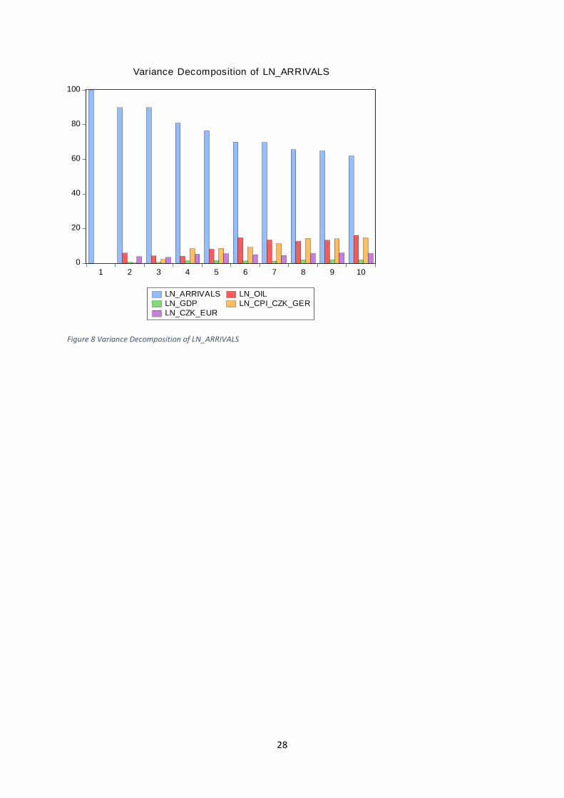
Figure 8 indicates the development of effect from exogenous variables on the number of German
tourists visiting the Czech Republic. It is obvious that in each quarter the importance of LN_ARRIVALS
is slightly decreasing and that there is an especially an impact of the variables LN_OIL and
LN_CPI_CZK_GER. Thus it is expected that in the next 10 quarters the arrivals will be mainly
influenced by the prices of oil and by the rate between consumer price indexes in the Czech Republic
and in Germany.
28
Figure 8 Variance Decomposition of LN_ARRIVALS
0
20
40
60
80
100
1 2 3 4 5 6 7 8 9 10
LN_ARRIVALS LN_OIL
LN_GDP LN_CPI_CZK_GER
LN_CZK_EUR
Variance Decomposition of LN_ARRIVALS
29
5 Discussion and Conclusion
Discussion
For more than two past decades the demand for tourism detected a huge development in tourism
researches. Just two dozen years ago only a few papers related to tourism demand and its analysis
were written. Nowadays according to Song and Li there are more than 70 journals related to tourism
demand and about 3000 institutions focusing on the tourism research – tourism demand modelling
plus its influencing variables and forecasting. Many researches used to use the approach of time
series model, as the endogenous variable was explained by its own past and a random disturbance
term. Most of them used ARIMA model or Garch models. Now the trend is to use the econometric
approaches because their main advantage is to analyze the causal relationship between the
endogenous variable (tourism demand) and other exogenous variables. Using the traditional
regression analysis (OLS) might end up with the spurious regression but a great development has
been done since and it is possible to use ADL, VAR or VEC model to analyze the tourism demand and
its forecast avoiding the spurious issue.
The aim of this paper is to analyze the German tourism demand for the Czech Republic using a
cointegration analysis and to find out the possible impacts of the selected variables on the number of
German tourists in the future. The reason is that there has never been undertaken any similar
empirical analysis of demand for the Czech Republic. The analysis of tourism demand for the Czech
Republic will show significant factors that have effects on its value and will help to explore the
impacts of shocks on exogenous variables effecting the number of arrivals.
In the research the ADF test is used to test the stationarity of all time series. It was proved that all
data have a non-stationary character but the time series become stationary after their first
differences. Then Johansen´s cointegration analysis is carried out to indicate whether there are any
cointegrative relationships among the variables and when it was confirmed the Vector error
correction model was estimated to examine a long-run causality and short-term relationship
between the tourism demand and other selected variables, specifically prices of oil, German GDP,
Consumer price Index between the Czech Republic and German and finally the exchange rate.
Results show that a short run change in GDP does not have a significant effect on the arrival of
German tourists. In the research of Lelwala and Gunaratne (2008) estimating the tourism demand for
Sri Lanka by United Kingdom tourists the GDP in UK was insignificant as well. The reason could be
that tourists are more income elastic in the long-run (Song and Witt, 2004). The Wald test showed
that the exchange rate CZK/EUR does not have any significant short effect on the number of arrivals

30
to the Czech Republic. On the other hand CPI and price of oil have a short run effect on the tourist
arrival as both values have significant levels. According to Nathakumar and Ibrahim (2007) Consumer
Price Index has the most dominant influence on the tourism demand which indicates the low
domestic price level in the Czech Republic and which was proved in our VEC model as well. As shown
in the error correction model the error correction term was estimated as -0.29. This speed of
adjustment is negative and significant. This coefficient guarantees the convergence of the time series
in long-run, thus a deviation of German tourists in the Czech Republic from a long-run equilibrium
will be corrected by 29% in the next quarter. The results of long run showed that variables are
significant in 10% probability except of GDP. Only price of oil has a positive sign which was not
expected according to the economic theory. Therefore the increase of price for oil means an increase
of tourist arrivals. In the research of Dritsakis (2004) it was proved that price of transportation cost
have a significant negative influence on the USA tourism demand for Greece but it might be
connected to the distance between these two countries. Our result showed the opposite. One of the
explanation might be that an increase of oil means more expensive flight tickets so people would
prefer going to neighbor countries by car instead of flying to further distances. That is visible from
the Impulse Response function as well for next ten quarters. That function shows the increase of
tourists visiting the Czech Republic as an impact of the increase of oil price. The negative signs of
Consumer Price Index between CZE and Germany and exchange rate indicate a negative influence on
the tourism demand, prices of goods and services in the Czech Republic are more expensive
comparing to Germany and exchange rate is not so favourable.
The results will help tourism policy makers and planners in the Czech Republic to adjust their
processes and plans to be more efficient in order to gain a competitive advantage. In our case the
tourists are sensitive to tourism prices, policy makers and suppliers should closely focus on all
tourism services and their prices to ensure that the prices remain affordable. Impulse Response
analysis estimated that the shocks on the individual variables and their impacts on the tourism
demand is not strong so it will not fluctuate a lot in the 10 quarters future. Thus it could be said that
the Germand tourism demand for the Czech Republic will be quite robust and the Czech tourism
sector can invest to German tourists safely. The second method of forecasting showed that during
next 10 quarters there will be some influence of the price of oil and the tourist prices on the number
of incoming German tourists.
There are various methods by which tourism demand can be analyzed. In this study focus was on the
coinegration analysis and VEC model. If the cointegration had not been confirmed, then the VAR
model would have been used. Our model chose five main variables – tourist arrivals as the main one
31
and other four explaining variables. But in many researches instead of tourism arrivals they used a
tourism expenditure as the endogenous variable. Although our model indicates a high R2 and all
diagnostic tests were significant and desirable, including some other variables might bring even
better results (the model showed that the GDP variable was not significant). On the other hand there
are no statistic records because some variables do not have a quantitative character. An example of
these could be political structures, countries preferences, different tastes or expectations, weather
and habit persistence. Furthermore it was used a quarter time series data but having monthly data
might bring better and more detailed analysis.
The choice for analyzing German tourism demand was made because so far Germans create the
largest group of incoming tourists to the Czech Republic, although recently there was a huge increase
of tourists coming from Asian countries. This Asian group is not so significant in the number of
tourists but they belong to a group of tourists who spend most money. Further analysis of tourism
demand should focus on that sector because it will have more importance in next years for Czech
tourism and it can be challenging to analyze less stable demand from Asian countries. These analysis
should consider that the tourists’ expenditure would be a main variable and not the number of
visitors.
Conclusion
Based on the analysis we can conclude that almost all selected variables had a significant long-term
effect on the German tourism demand for the Czech Republic, except of German GDP. From the
economic point of view the signs of variables are correct at the rate of Consumer prices indexes and
the exchange rate. On the other hand the oil indicates the contrary but it can be explained at some
point as well. The results from the first used forecast method show that the number of arrivals will
not fluctuate a lot during next quarter, meaning that the German tourism demand will be quite
stable. From the second method it was estimated that the demand would be more and more
influenced by the price of oil and tourism prices.

32
33
6 References
Brooks, C. (2002). Introductory econometrics for finance. Cambridge: Cambridge University Press.
"Česká Republika Od Roku 1989 V Číslech". Český Statistický Úřad. N.p., 2016. Web. 7 Feb. 2016.
Český Statistický Úřad,. Návštěvnost V Hromadných Ubytovacích Zařízeních V ČR. Cestovní Ruch –
Časové Řady. 2015. Web. 17 Feb. 2016.
Cipra, T. (2008). Financní ekonometrie. Praha: Ekopress.
Crouch, G. I. "The Study Of International Tourism Demand: A Review Of Findings". Journal of Travel
Research 33.1 (1994): 12-23. Web.
Czech Statistical Office,. Number Of Guests In Collective Accommodation Establishments By Country
In The Czech Republic And Regions. 2016. Print. Tourism - Time Series.
Dritsakis, Nikolaos. "Cointegration Analysis Of German And British Tourism Demand For
Greece". Tourism Management 25.1 (2004): 111-119. Web.
Engle, Robert F. and C. W. J. Granger. "Co-Integration And Error Correction: Representation,
Estimation, And Testing". Econometrica 55.2 (1987): 251. Web.
Gounoploulos, D., Petmezas, D. and Santamaria, D. (2012) Forecasting tourist arrivals in Greece and
the impact of macroeconomic shocks from the countries of tourists' origin. Annals of Tourism
Research, 39 (2). pp. 641-666. ISSN 0160-7383.
Ioannides, Dimitri, and Keith G Debbage. The Economic Geography Of The Tourist Industry. London:
Routledge, 1998. Print.
Johansen, Søren and Katarina Juselius. "MAXIMUM LIKELIHOOD ESTIMATION AND INFERENCE ON
COINTEGRATION - WITH APPLICATIONS TO THE DEMAND FOR MONEY". Oxford Bulletin of Economics
and Statistics 52.2 (2009): 169-210. Web.
Johansen, S. Statistical analysis of cointegration vectors. Journal of Economic Dynamics and Control,
12, (1988), 231–254.
Hardy, Melissa A. Regression With Dummy Variables. Newbury Park, Calif.: Sage Publications, 1993.
Print.
"Kapacita Hromadných Ubytovacích Zařízení". Český Statistický Úřad. N.p., 2016. Web. 8 Feb. 2016.
Kocenda, E., Černý, A., Kodera, J., Vosvrda, M. and Havlícek, J. (n.d.). Elements of time series
econometrics. Prague: Karolinum Press, 2015.
Lim, Christine and Michael McAleer. "A Seasonal Analysis Of Asian Tourist Arrivals To
Australia". Applied Economics 32.4 (2000): 499-509. Web.
Lelwala, E.I. and L.H.P. Gunaratne. "Modelling Tourism Demand Using Cointegration Analysis: A Case
Study For Tourists Arriving From United Kingdom To Sri Lanka". Tropical Agricultural Research 20
(2008): 50-59. Print.
Matias, Alvaro, Peter Nijkamp, and Manuela Sarmento. Advances In Tourism Economics. Heidelberg:
Physica-Verlag, 2009. Print.
34
Middleton, Michael R. Data Analysis Using Microsoft Excel. Belmont, CA: Duxbury Press, 1997. Print.
Morley, Clive L. "A Microeconomic Theory Of International Tourism Demand". Annals of Tourism
Research 19.2 (1992): 250-267. Web.
Nathakumar, L. and Y. Ibrahim. "Tourism Development Policy, Strategic Alliances And Impact Of
Consumer Price Index On Tourist Arrivals: The Case Of Malaysia". MPRA (2007): n. pag. Print.
Palatková, Monika. Marketingový Management Destinací. Praha: Grada, 2011. Print.
Palatková, Monika. Mezinárodní Turismus. Praha: Grada, 2014. Print.
Palatková, Monika and Táňa Valská. Marketingové Strategie (Country Reporty Za Rok 2014). Praha:
Czech Tourism, 2014. Print.
Song, H. and Li, G. (2008). Tourism demand modelling and forecasting—A review of recent
research. Tourism Management, 29(2), pp.203-220.
Song, H. and Witt, S. (2000). Tourism demand modelling and forecasting. Amsterdam: Pergamon.
Tittelbachová, Sárka. Turismus A Veřejná Správa. Praha: Grada, 2011. Print.
Tsay, Ruey S. Analysis Of Financial Time Series. New York: Wiley, 2002. Print.
Vanek, Miroslav, and PavelMucke. Velvet Revolutions. An Oral History Of Czech Society. Corby:
Oxford University Press, 2015. Print.
VYSTOUPIL, Jiří. Vývoj cestovního ruchu v ČR a jeho prostorové organizace v letech 1990 - 2009.
Urbanismus a územní rozvoj. Brno, Ústav územního rozvoje, 2010, vol. 13, no. 5. Print.
Witt, S. and C.A. Marin. "Tourism Demand Forecasting Models: Choice Of Appropriate Variable To
Represent Tourists' Cost Of Living". Tourism Management 8 (2016): 233-246. Print.
Online references:
"Introduction To Cointegration And Pairs Trading". Blog.echen.me. N.p., 2016. Web. 17 Apr. 2016.
Czso.cz,. "Cestovní Ruch – Časové Řady | ČSÚ". N.p., 2015. Web. 22 Dec. 2015.
Czechtourism.cz. (2016). Monitoring zahranicních turistů v návaznosti na geografické clenění -
Zámoří. [online] Available at: http://www.czechtourism.cz/getmedia/91063396-29b1-4061-bf0f-
e75ef2addf4d/03_09_14_zamori_zaverecna_zprava.pdf.aspx [Accessed 23 Apr. 2016].
Ec.europa.eu. (2016). Národní úcty a HDP – Statistics Explained. [online] Available at:
http://ec.europa.eu/eurostat/statistics-explained/index.php/National_accounts_and_GDP/cs
[Accessed 23 Mar. 2016].
Eviews.com. (2016). EViews.com. [online] Available at: http://www.eviews.com/home.html
[Accessed 6 Apr. 2016].
Www2.unwto.org. (2016). UNWTO Annual Report 2013 | World Tourism Organization UNWTO.
[online] Available at: http://www2.unwto.org/publication/unwto-annual-report-2013 [Accessed 14
Apr. 2016].
35
Www2.unwto.org. (2016). UNWTO Annual Report 2010 | World Tourism Organization UNWTO.
[online] Available at: http://www2.unwto.org/publication/unwto-annual-report-2010 [Accessed 14
Apr. 2016].
Www2.unwto.org. (2016). UNWTO Annual Report 2014 | World Tourism Organization UNWTO.
[online] Available at: http://www2.unwto.org/publication/unwto-annual-report-2014 [Accessed 14
Apr. 2016].

36
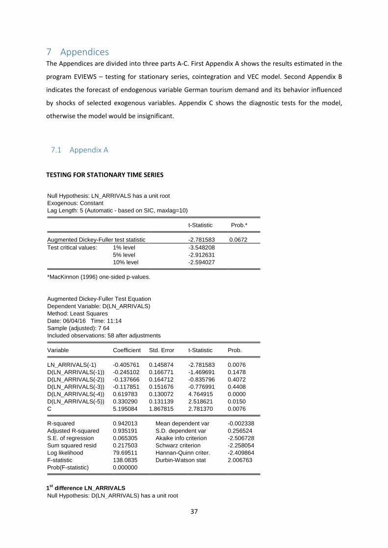
37
7 Appendices The Appendices are divided into three parts A-C. First Appendix A shows the results estimated in the
program EVIEWS – testing for stationary series, cointegration and VEC model. Second Appendix B
indicates the forecast of endogenous variable German tourism demand and its behavior influenced
by shocks of selected exogenous variables. Appendix C shows the diagnostic tests for the model,
otherwise the model would be insignificant.
7.1 Appendix A
TESTING FOR STATIONARY TIME SERIES
Null Hypothesis: LN_ARRIVALS has a unit root
Exogenous: Constant
Lag Length: 5 (Automatic - based on SIC, maxlag=10) t-Statistic Prob.* Augmented Dickey-Fuller test statistic -2.781583 0.0672
Test critical values: 1% level -3.548208
5% level -2.912631
10% level -2.594027 *MacKinnon (1996) one-sided p-values.
Augmented Dickey-Fuller Test Equation
Dependent Variable: D(LN_ARRIVALS)
Method: Least Squares
Date: 06/04/16 Time: 11:14
Sample (adjusted): 7 64
Included observations: 58 after adjustments Variable Coefficient Std. Error t-Statistic Prob. LN_ARRIVALS(-1) -0.405761 0.145874 -2.781583 0.0076
D(LN_ARRIVALS(-1)) -0.245102 0.166771 -1.469691 0.1478
D(LN_ARRIVALS(-2)) -0.137666 0.164712 -0.835796 0.4072
D(LN_ARRIVALS(-3)) -0.117851 0.151676 -0.776991 0.4408
D(LN_ARRIVALS(-4)) 0.619783 0.130072 4.764915 0.0000
D(LN_ARRIVALS(-5)) 0.330290 0.131139 2.518621 0.0150
C 5.195084 1.867815 2.781370 0.0076 R-squared 0.942013 Mean dependent var -0.002338
Adjusted R-squared 0.935191 S.D. dependent var 0.256524
S.E. of regression 0.065305 Akaike info criterion -2.506728
Sum squared resid 0.217503 Schwarz criterion -2.258054
Log likelihood 79.69511 Hannan-Quinn criter. -2.409864
F-statistic 138.0835 Durbin-Watson stat 2.006763
Prob(F-statistic) 0.000000 1
st difference LN_ARRIVALS
Null Hypothesis: D(LN_ARRIVALS) has a unit root
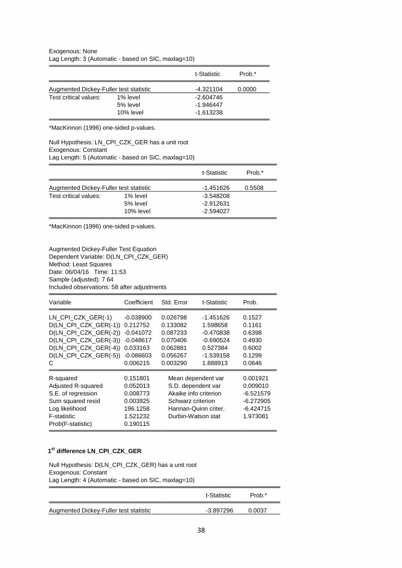
38
Exogenous: None
Lag Length: 3 (Automatic - based on SIC, maxlag=10) t-Statistic Prob.* Augmented Dickey-Fuller test statistic -4.321104 0.0000
Test critical values: 1% level -2.604746
5% level -1.946447
10% level -1.613238 *MacKinnon (1996) one-sided p-values.
Null Hypothesis: LN_CPI_CZK_GER has a unit root
Exogenous: Constant
Lag Length: 5 (Automatic - based on SIC, maxlag=10) t-Statistic Prob.* Augmented Dickey-Fuller test statistic -1.451626 0.5508
Test critical values: 1% level -3.548208
5% level -2.912631
10% level -2.594027 *MacKinnon (1996) one-sided p-values.
Augmented Dickey-Fuller Test Equation
Dependent Variable: D(LN_CPI_CZK_GER)
Method: Least Squares
Date: 06/04/16 Time: 11:53
Sample (adjusted): 7 64
Included observations: 58 after adjustments Variable Coefficient Std. Error t-Statistic Prob. LN_CPI_CZK_GER(-1) -0.038900 0.026798 -1.451626 0.1527
D(LN_CPI_CZK_GER(-1)) 0.212752 0.133082 1.598658 0.1161
D(LN_CPI_CZK_GER(-2)) -0.041072 0.087233 -0.470838 0.6398
D(LN_CPI_CZK_GER(-3)) -0.048617 0.070406 -0.690524 0.4930
D(LN_CPI_CZK_GER(-4)) 0.033163 0.062881 0.527384 0.6002
D(LN_CPI_CZK_GER(-5)) -0.086603 0.056267 -1.539158 0.1299
C 0.006215 0.003290 1.888913 0.0646 R-squared 0.151801 Mean dependent var 0.001921
Adjusted R-squared 0.052013 S.D. dependent var 0.009010
S.E. of regression 0.008773 Akaike info criterion -6.521579
Sum squared resid 0.003925 Schwarz criterion -6.272905
Log likelihood 196.1258 Hannan-Quinn criter. -6.424715
F-statistic 1.521232 Durbin-Watson stat 1.973081
Prob(F-statistic) 0.190115
1st
difference LN_CPI_CZK_GER
Null Hypothesis: D(LN_CPI_CZK_GER) has a unit root
Exogenous: Constant
Lag Length: 4 (Automatic - based on SIC, maxlag=10) t-Statistic Prob.* Augmented Dickey-Fuller test statistic -3.897296 0.0037
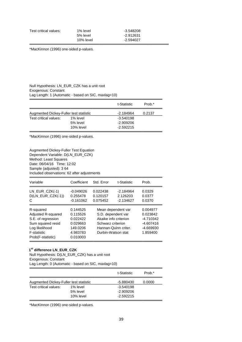
39
Test critical values: 1% level -3.548208
5% level -2.912631
10% level -2.594027 *MacKinnon (1996) one-sided p-values.
Null Hypothesis: LN_EUR_CZK has a unit root
Exogenous: Constant
Lag Length: 1 (Automatic - based on SIC, maxlag=10) t-Statistic Prob.* Augmented Dickey-Fuller test statistic -2.184964 0.2137
Test critical values: 1% level -3.540198
5% level -2.909206
10% level -2.592215 *MacKinnon (1996) one-sided p-values.
Augmented Dickey-Fuller Test Equation
Dependent Variable: D(LN_EUR_CZK)
Method: Least Squares
Date: 06/04/16 Time: 12:02
Sample (adjusted): 3 64
Included observations: 62 after adjustments Variable Coefficient Std. Error t-Statistic Prob. LN_EUR_CZK(-1) -0.049026 0.022438 -2.184964 0.0329
D(LN_EUR_CZK(-1)) 0.255478 0.120157 2.126203 0.0377
C -0.161062 0.075452 -2.134627 0.0370 R-squared 0.144525 Mean dependent var 0.004977
Adjusted R-squared 0.115526 S.D. dependent var 0.023842
S.E. of regression 0.022422 Akaike info criterion -4.710342
Sum squared resid 0.029663 Schwarz criterion -4.607416
Log likelihood 149.0206 Hannan-Quinn criter. -4.669930
F-statistic 4.983783 Durbin-Watson stat 1.859400
Prob(F-statistic) 0.010003 1
st difference LN_EUR_CZK
Null Hypothesis: D(LN_EUR_CZK) has a unit root
Exogenous: Constant
Lag Length: 0 (Automatic - based on SIC, maxlag=10) t-Statistic Prob.* Augmented Dickey-Fuller test statistic -5.880430 0.0000
Test critical values: 1% level -3.540198
5% level -2.909206
10% level -2.592215 *MacKinnon (1996) one-sided p-values.
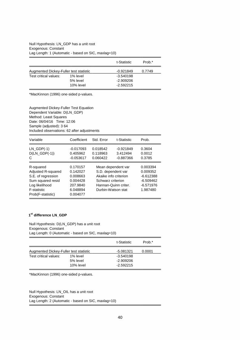
40
Null Hypothesis: LN_GDP has a unit root
Exogenous: Constant
Lag Length: 1 (Automatic - based on SIC, maxlag=10) t-Statistic Prob.* Augmented Dickey-Fuller test statistic -0.921849 0.7749
Test critical values: 1% level -3.540198
5% level -2.909206
10% level -2.592215 *MacKinnon (1996) one-sided p-values.
Augmented Dickey-Fuller Test Equation
Dependent Variable: D(LN_GDP)
Method: Least Squares
Date: 06/04/16 Time: 12:06
Sample (adjusted): 3 64
Included observations: 62 after adjustments Variable Coefficient Std. Error t-Statistic Prob. LN_GDP(-1) -0.017093 0.018542 -0.921849 0.3604
D(LN_GDP(-1)) 0.405962 0.118963 3.412494 0.0012
C -0.053617 0.060422 -0.887366 0.3785 R-squared 0.170157 Mean dependent var 0.003394
Adjusted R-squared 0.142027 S.D. dependent var 0.009352
S.E. of regression 0.008663 Akaike info criterion -6.612388
Sum squared resid 0.004428 Schwarz criterion -6.509462
Log likelihood 207.9840 Hannan-Quinn criter. -6.571976
F-statistic 6.048894 Durbin-Watson stat 1.987480
Prob(F-statistic) 0.004077
1st
difference LN_GDP
Null Hypothesis: D(LN_GDP) has a unit root
Exogenous: Constant
Lag Length: 0 (Automatic - based on SIC, maxlag=10) t-Statistic Prob.* Augmented Dickey-Fuller test statistic -5.081321 0.0001
Test critical values: 1% level -3.540198
5% level -2.909206
10% level -2.592215 *MacKinnon (1996) one-sided p-values.
Null Hypothesis: LN_OIL has a unit root
Exogenous: Constant
Lag Length: 2 (Automatic - based on SIC, maxlag=10)
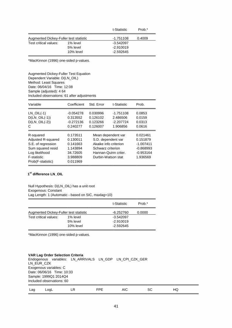
41
t-Statistic Prob.* Augmented Dickey-Fuller test statistic -1.751108 0.4009
Test critical values: 1% level -3.542097
5% level -2.910019
10% level -2.592645 *MacKinnon (1996) one-sided p-values.
Augmented Dickey-Fuller Test Equation
Dependent Variable: D(LN_OIL)
Method: Least Squares
Date: 06/04/16 Time: 12:08
Sample (adjusted): 4 64
Included observations: 61 after adjustments Variable Coefficient Std. Error t-Statistic Prob. LN_OIL(-1) -0.054278 0.030996 -1.751108 0.0853
D(LN_OIL(-1)) 0.313552 0.126102 2.486506 0.0159
D(LN_OIL(-2)) -0.272136 0.123266 -2.207724 0.0313
C 0.240277 0.126007 1.906856 0.0616 R-squared 0.173511 Mean dependent var 0.021461
Adjusted R-squared 0.130011 S.D. dependent var 0.151879
S.E. of regression 0.141663 Akaike info criterion -1.007411
Sum squared resid 1.143894 Schwarz criterion -0.868993
Log likelihood 34.72605 Hannan-Quinn criter. -0.953164
F-statistic 3.988809 Durbin-Watson stat 1.936569
Prob(F-statistic) 0.011969
1st
difference LN_OIL
Null Hypothesis: D(LN_OIL) has a unit root
Exogenous: Constant
Lag Length: 1 (Automatic - based on SIC, maxlag=10) t-Statistic Prob.* Augmented Dickey-Fuller test statistic -6.252760 0.0000
Test critical values: 1% level -3.542097
5% level -2.910019
10% level -2.592645 *MacKinnon (1996) one-sided p-values.
VAR Lag Order Selection Criteria Endogenous variables: LN_ARRIVALS LN_GDP LN_CPI_CZK_GER LN_EUR_CZK
Exogenous variables: C
Date: 06/06/16 Time: 10:33
Sample: 1999Q1 2014Q4
Included observations: 60 Lag LogL LR FPE AIC SC HQ
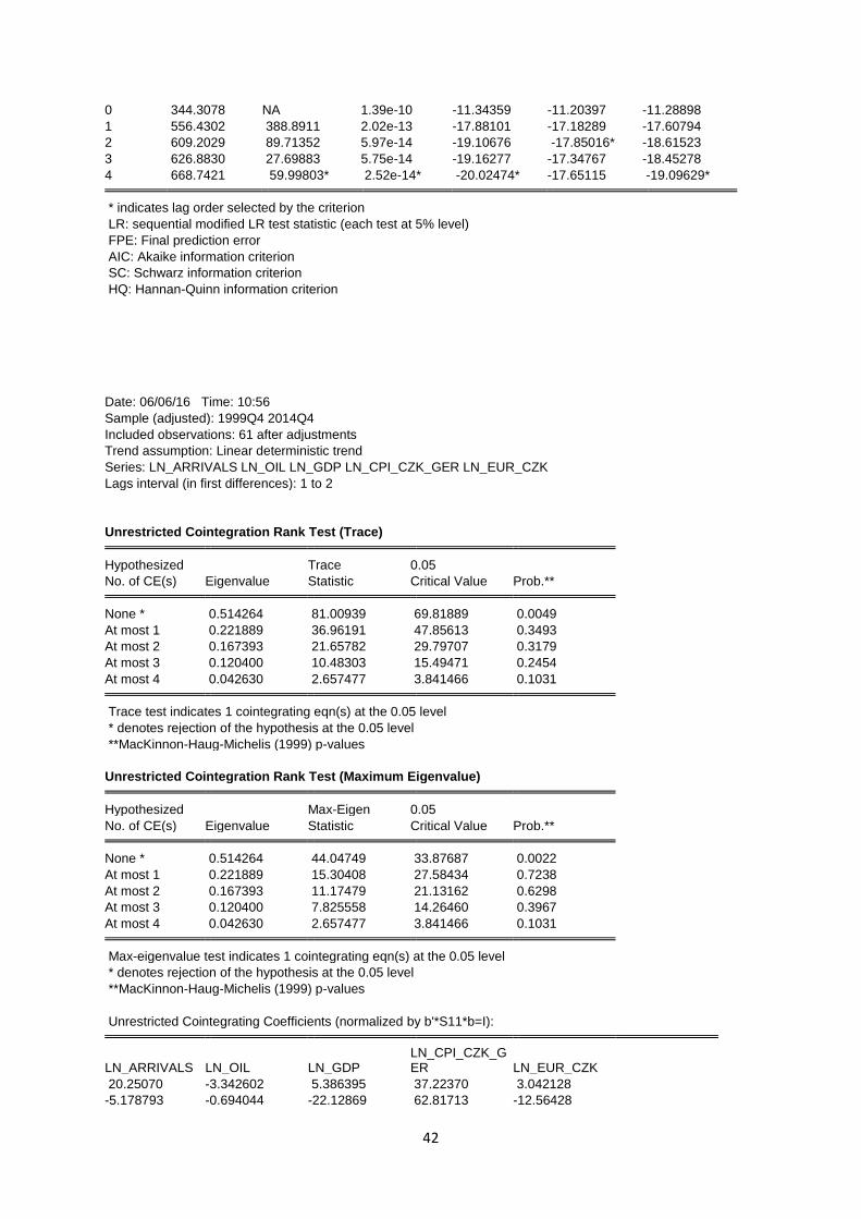
42
0 344.3078 NA 1.39e-10 -11.34359 -11.20397 -11.28898
1 556.4302 388.8911 2.02e-13 -17.88101 -17.18289 -17.60794
2 609.2029 89.71352 5.97e-14 -19.10676 -17.85016* -18.61523
3 626.8830 27.69883 5.75e-14 -19.16277 -17.34767 -18.45278
4 668.7421 59.99803* 2.52e-14* -20.02474* -17.65115 -19.09629* * indicates lag order selected by the criterion
LR: sequential modified LR test statistic (each test at 5% level)
FPE: Final prediction error
AIC: Akaike information criterion
SC: Schwarz information criterion
HQ: Hannan-Quinn information criterion
Date: 06/06/16 Time: 10:56
Sample (adjusted): 1999Q4 2014Q4
Included observations: 61 after adjustments
Trend assumption: Linear deterministic trend
Series: LN_ARRIVALS LN_OIL LN_GDP LN_CPI_CZK_GER LN_EUR_CZK
Lags interval (in first differences): 1 to 2
Unrestricted Cointegration Rank Test (Trace) Hypothesized Trace 0.05
No. of CE(s) Eigenvalue Statistic Critical Value Prob.** None * 0.514264 81.00939 69.81889 0.0049
At most 1 0.221889 36.96191 47.85613 0.3493
At most 2 0.167393 21.65782 29.79707 0.3179
At most 3 0.120400 10.48303 15.49471 0.2454
At most 4 0.042630 2.657477 3.841466 0.1031 Trace test indicates 1 cointegrating eqn(s) at the 0.05 level
* denotes rejection of the hypothesis at the 0.05 level
**MacKinnon-Haug-Michelis (1999) p-values
Unrestricted Cointegration Rank Test (Maximum Eigenvalue) Hypothesized Max-Eigen 0.05
No. of CE(s) Eigenvalue Statistic Critical Value Prob.** None * 0.514264 44.04749 33.87687 0.0022
At most 1 0.221889 15.30408 27.58434 0.7238
At most 2 0.167393 11.17479 21.13162 0.6298
At most 3 0.120400 7.825558 14.26460 0.3967
At most 4 0.042630 2.657477 3.841466 0.1031 Max-eigenvalue test indicates 1 cointegrating eqn(s) at the 0.05 level
* denotes rejection of the hypothesis at the 0.05 level
**MacKinnon-Haug-Michelis (1999) p-values
Unrestricted Cointegrating Coefficients (normalized by b'*S11*b=I):
LN_ARRIVALS LN_OIL LN_GDP LN_CPI_CZK_GER LN_EUR_CZK
20.25070 -3.342602 5.386395 37.22370 3.042128
-5.178793 -0.694044 -22.12869 62.81713 -12.56428
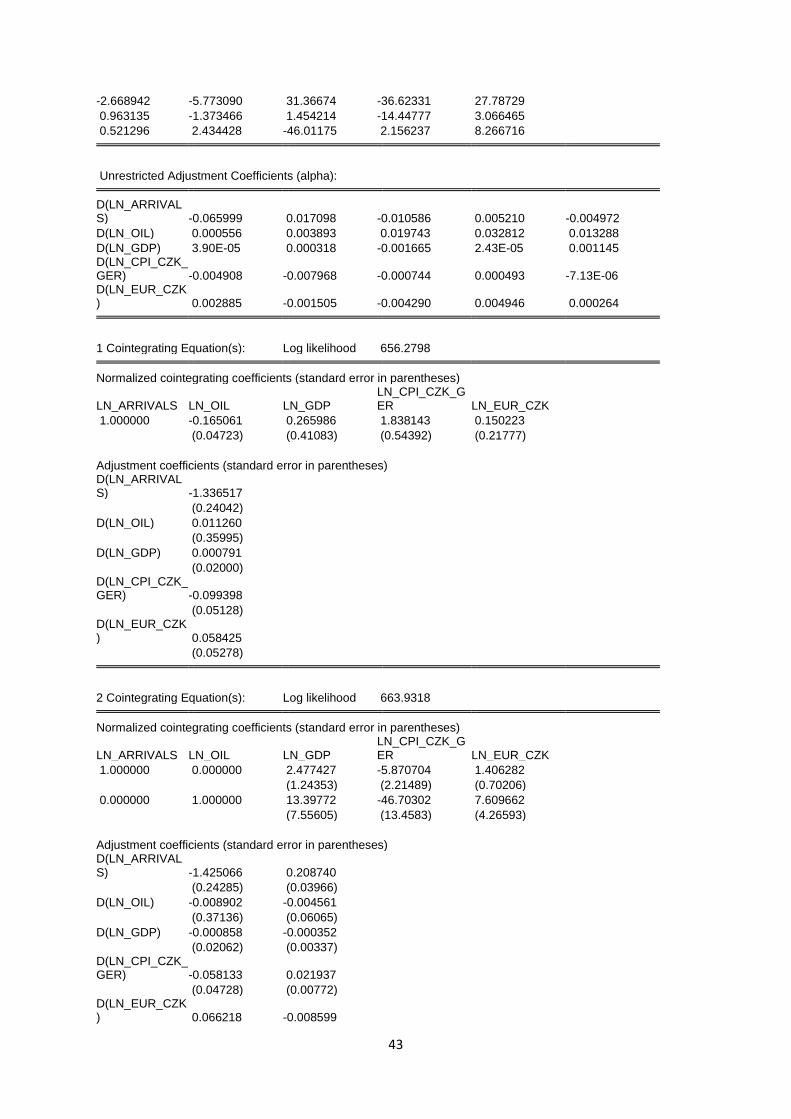
43
-2.668942 -5.773090 31.36674 -36.62331 27.78729
0.963135 -1.373466 1.454214 -14.44777 3.066465
0.521296 2.434428 -46.01175 2.156237 8.266716
Unrestricted Adjustment Coefficients (alpha): D(LN_ARRIVALS) -0.065999 0.017098 -0.010586 0.005210 -0.004972
D(LN_OIL) 0.000556 0.003893 0.019743 0.032812 0.013288
D(LN_GDP) 3.90E-05 0.000318 -0.001665 2.43E-05 0.001145 D(LN_CPI_CZK_GER) -0.004908 -0.007968 -0.000744 0.000493 -7.13E-06 D(LN_EUR_CZK) 0.002885 -0.001505 -0.004290 0.004946 0.000264
1 Cointegrating Equation(s): Log likelihood 656.2798 Normalized cointegrating coefficients (standard error in parentheses)
LN_ARRIVALS LN_OIL LN_GDP LN_CPI_CZK_GER LN_EUR_CZK
1.000000 -0.165061 0.265986 1.838143 0.150223
(0.04723) (0.41083) (0.54392) (0.21777)
Adjustment coefficients (standard error in parentheses) D(LN_ARRIVALS) -1.336517
(0.24042)
D(LN_OIL) 0.011260
(0.35995)
D(LN_GDP) 0.000791
(0.02000) D(LN_CPI_CZK_GER) -0.099398
(0.05128) D(LN_EUR_CZK) 0.058425
(0.05278)
2 Cointegrating Equation(s): Log likelihood 663.9318 Normalized cointegrating coefficients (standard error in parentheses)
LN_ARRIVALS LN_OIL LN_GDP LN_CPI_CZK_GER LN_EUR_CZK
1.000000 0.000000 2.477427 -5.870704 1.406282
(1.24353) (2.21489) (0.70206)
0.000000 1.000000 13.39772 -46.70302 7.609662
(7.55605) (13.4583) (4.26593)
Adjustment coefficients (standard error in parentheses) D(LN_ARRIVALS) -1.425066 0.208740
(0.24285) (0.03966)
D(LN_OIL) -0.008902 -0.004561
(0.37136) (0.06065)
D(LN_GDP) -0.000858 -0.000352
(0.02062) (0.00337) D(LN_CPI_CZK_GER) -0.058133 0.021937
(0.04728) (0.00772) D(LN_EUR_CZK) 0.066218 -0.008599
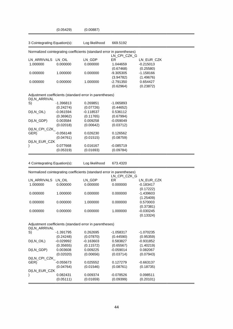
44
(0.05429) (0.00887)
3 Cointegrating Equation(s): Log likelihood 669.5192 Normalized cointegrating coefficients (standard error in parentheses)
LN_ARRIVALS LN_OIL LN_GDP LN_CPI_CZK_GER LN_EUR_CZK
1.000000 0.000000 0.000000 1.044659 -0.215013
(0.67468) (0.25580)
0.000000 1.000000 0.000000 -9.305305 -1.158166
(3.94782) (1.49676)
0.000000 0.000000 1.000000 -2.791350 0.654427
(0.62964) (0.23872)
Adjustment coefficients (standard error in parentheses) D(LN_ARRIVALS) -1.396813 0.269851 -1.065893
(0.24274) (0.07726) (0.44652)
D(LN_OIL) -0.061594 -0.118537 0.536112
(0.36962) (0.11765) (0.67994)
D(LN_GDP) 0.003584 0.009258 -0.059049
(0.02018) (0.00642) (0.03712) D(LN_CPI_CZK_GER) -0.056148 0.026230 0.126562
(0.04761) (0.01515) (0.08759) D(LN_EUR_CZK) 0.077668 0.016167 -0.085719
(0.05319) (0.01693) (0.09784)
4 Cointegrating Equation(s): Log likelihood 673.4320 Normalized cointegrating coefficients (standard error in parentheses)
LN_ARRIVALS LN_OIL LN_GDP LN_CPI_CZK_GER LN_EUR_CZK
1.000000 0.000000 0.000000 0.000000 -0.183417
(0.17222)
0.000000 1.000000 0.000000 0.000000 -1.439603
(1.25409)
0.000000 0.000000 1.000000 0.000000 0.570003
(0.37381)
0.000000 0.000000 0.000000 1.000000 -0.030245
(0.13324)
Adjustment coefficients (standard error in parentheses) D(LN_ARRIVALS) -1.391795 0.262695 -1.058317 -1.070235
(0.24248) (0.07870) (0.44590) (0.95359)
D(LN_OIL) -0.029992 -0.163603 0.583827 -0.931852
(0.35655) (0.11572) (0.65567) (1.40219)
D(LN_GDP) 0.003608 0.009225 -0.059014 0.082067
(0.02020) (0.00656) (0.03714) (0.07943) D(LN_CPI_CZK_GER) -0.055673 0.025552 0.127279 -0.663137
(0.04764) (0.01546) (0.08761) (0.18735) D(LN_EUR_CZK) 0.082431 0.009374 -0.078526 0.098511
(0.05111) (0.01659) (0.09399) (0.20101)
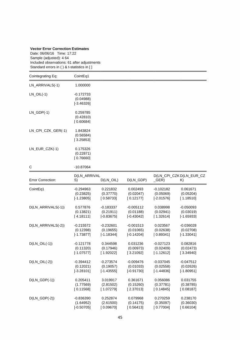
45
Vector Error Correction Estimates
Date: 06/06/16 Time: 17:22
Sample (adjusted): 4 64
Included observations: 61 after adjustments
Standard errors in ( ) & t-statistics in [ ] Cointegrating Eq: CointEq1 LN_ARRIVALS(-1) 1.000000
LN_OIL(-1) -0.172733
(0.04988)
[-3.46326]
LN_GDP(-1) 0.259785
(0.42810)
[ 0.60684]
LN_CPI_CZK_GER(-1) 1.843824
(0.56584)
[ 3.25853]
LN_EUR_CZK(-1) 0.175326
(0.22871)
[ 0.76660]
C -10.87064
Error Correction: D(LN_ARRIVALS) D(LN_OIL) D(LN_GDP)
D(LN_CPI_CZK_GER)
D(LN_EUR_CZK)
CointEq1 -0.294963 0.221832 0.002493 -0.102182 0.061671
(0.23825) (0.37770) (0.02047) (0.05069) (0.05204)
[-1.23805] [ 0.58733] [ 0.12177] [-2.01576] [ 1.18510]
D(LN_ARRIVALS(-1)) 0.577876 -0.183337 -0.005112 0.038998 -0.050093
(0.13821) (0.21911) (0.01188) (0.02941) (0.03019)
[ 4.18111] [-0.83675] [-0.43042] [ 1.32614] [-1.65933]
D(LN_ARRIVALS(-2)) -0.215572 -0.232601 -0.001513 0.023567 -0.036028
(0.12398) (0.19655) (0.01065) (0.02638) (0.02708)
[-1.73877] [-1.18344] [-0.14204] [ 0.89341] [-1.33041]
D(LN_OIL(-1)) -0.121778 0.344598 0.031236 -0.027123 0.082816
(0.11320) (0.17946) (0.00973) (0.02409) (0.02473)
[-1.07577] [ 1.92022] [ 3.21092] [-1.12612] [ 3.34940]
D(LN_OIL(-2)) -0.394412 -0.273574 -0.009476 -0.037045 -0.047512
(0.12021) (0.19057) (0.01033) (0.02558) (0.02626)
[-3.28101] [-1.43555] [-0.91730] [-1.44836] [-1.80951]
D(LN_GDP(-1)) 0.205411 3.019917 0.361671 0.056086 0.031755
(1.77569) (2.81502) (0.15260) (0.37781) (0.38785)
[ 0.11568] [ 1.07279] [ 2.37013] [ 0.14845] [ 0.08187]
D(LN_GDP(-2)) -0.836390 0.252874 0.079968 0.270259 0.238170
(1.64952) (2.61500) (0.14175) (0.35097) (0.36030)
[-0.50705] [ 0.09670] [ 0.56413] [ 0.77004] [ 0.66104]
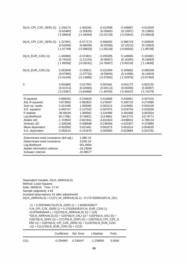
46
D(LN_CPI_CZK_GER(-1)) 2.156174 -1.402281 -0.012938 -0.436857 -0.012505
(0.63480) (1.00635) (0.05455) (0.13507) (0.13865)
[ 3.39664] [-1.39344] [-0.23716] [-3.23441] [-0.09018]
D(LN_CPI_CZK_GER(-2)) 1.227901 -0.577173 -0.056092 -0.086724 0.269505
(0.62094) (0.98438) (0.05336) (0.13212) (0.13563)
[ 1.97748] [-0.58633] [-1.05118] [-0.65642] [ 1.98708]
D(LN_EUR_CZK(-1)) 1.446960 -0.474811 -0.050285 0.146696 0.191691
(0.76423) (1.21154) (0.06567) (0.16260) (0.16693)
[ 1.89336] [-0.39191] [-0.76567] [ 0.90216] [ 1.14836]
D(LN_EUR_CZK(-2)) 0.281609 0.150611 -0.021959 0.336865 -0.085338
(0.67956) (1.07732) (0.05840) (0.14459) (0.14843)
[ 0.41440] [ 0.13980] [-0.37602] [ 2.32978] [-0.57492]
C 0.002885 0.017052 0.001691 0.001273 0.002132
(0.01314) (0.02083) (0.00113) (0.00280) (0.00287)
[ 0.21957] [ 0.81869] [ 1.49763] [ 0.45537] [ 0.74279] R-squared 0.896252 0.234628 0.410699 0.433001 0.407410
Adj. R-squared 0.872962 0.062810 0.278407 0.305715 0.274380
Sum sq. resids 0.421495 1.059305 0.003113 0.019081 0.020109
S.E. equation 0.092747 0.147032 0.007970 0.019734 0.020258
F-statistic 38.48169 1.365562 3.104489 3.401808 3.062534
Log likelihood 65.17681 37.06921 214.8802 159.5770 157.9771
Akaike AIC -1.743502 -0.821941 -6.651810 -4.838591 -4.786134
Schwarz SC -1.328248 -0.406688 -6.236556 -4.423337 -4.370880
Mean dependent -0.003065 0.021461 0.003275 0.001814 0.004535
S.D. dependent 0.260214 0.151879 0.009383 0.023683 0.023782 Determinant resid covariance (dof adj.) 1.08E-15
Determinant resid covariance 3.62E-16
Log likelihood 651.6694
Akaike information criterion -19.23506
Schwarz criterion -16.98577
Dependent Variable: D(LN_ARRIVALS)
Method: Least Squares
Date: 06/06/16 Time: 17:47
Sample (adjusted): 4 64
Included observations: 61 after adjustments
D(LN_ARRIVALS) = C(1)*( LN_ARRIVALS(-1) - 0.172732584169*LN_OIL(
-1) + 0.259784817513*LN_GDP(-1) + 1.84382436977
*LN_CPI_CZK_GER(-1) + 0.17532643515*LN_EUR_CZK(-1) -
10.8706435444 ) + C(2)*D(LN_ARRIVALS(-1)) + C(3)
*D(LN_ARRIVALS(-2)) + C(4)*D(LN_OIL(-1)) + C(5)*D(LN_OIL(-2)) +
C(6)*D(LN_GDP(-1)) + C(7)*D(LN_GDP(-2)) + C(8)*D(LN_CPI_CZK_G
ER(-1)) + C(9)*D(LN_CPI_CZK_GER(-2)) + C(10)*D(LN_EUR_CZK(
-1)) + C(11)*D(LN_EUR_CZK(-2)) + C(12) Coefficient Std. Error t-Statistic Prob. C(1) -0.294963 0.238247 -1.238055 0.0000
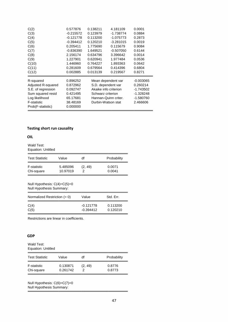
47
C(2) 0.577876 0.138211 4.181109 0.0001
C(3) -0.215572 0.123979 -1.738774 0.0884
C(4) -0.121778 0.113200 -1.075773 0.2873
C(5) -0.394412 0.120210 -3.281015 0.0019
C(6) 0.205411 1.775690 0.115679 0.9084
C(7) -0.836390 1.649521 -0.507050 0.6144
C(8) 2.156174 0.634796 3.396642 0.0014
C(9) 1.227901 0.620941 1.977484 0.0536
C(10) 1.446960 0.764227 1.893363 0.0642
C(11) 0.281609 0.679564 0.414396 0.6804
C(12) 0.002885 0.013139 0.219567 0.8271 R-squared 0.896252 Mean dependent var -0.003065
Adjusted R-squared 0.872962 S.D. dependent var 0.260214
S.E. of regression 0.092747 Akaike info criterion -1.743502
Sum squared resid 0.421495 Schwarz criterion -1.328248
Log likelihood 65.17681 Hannan-Quinn criter. -1.580760
F-statistic 38.48169 Durbin-Watson stat 2.466606
Prob(F-statistic) 0.000000
Testing short run causality
OIL
Wald Test:
Equation: Untitled Test Statistic Value df Probability F-statistic 5.485096 (2, 49) 0.0071
Chi-square 10.97019 2 0.0041
Null Hypothesis: C(4)=C(5)=0
Null Hypothesis Summary: Normalized Restriction (= 0) Value Std. Err. C(4) -0.121778 0.113200
C(5) -0.394412 0.120210 Restrictions are linear in coefficients.
GDP
Wald Test:
Equation: Untitled Test Statistic Value df Probability F-statistic 0.130871 (2, 49) 0.8776
Chi-square 0.261742 2 0.8773
Null Hypothesis: C(6)=C(7)=0
Null Hypothesis Summary:
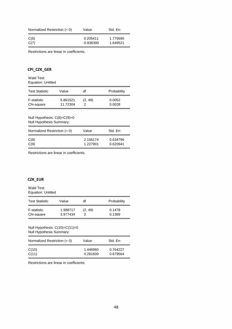
48
Normalized Restriction (= 0) Value Std. Err. C(6) 0.205411 1.775690
C(7) -0.836390 1.649521 Restrictions are linear in coefficients.
CPI_CZK_GER
Wald Test:
Equation: Untitled Test Statistic Value df Probability F-statistic 5.861521 (2, 49) 0.0052
Chi-square 11.72304 2 0.0028
Null Hypothesis: C(8)=C(9)=0
Null Hypothesis Summary: Normalized Restriction (= 0) Value Std. Err. C(8) 2.156174 0.634796
C(9) 1.227901 0.620941 Restrictions are linear in coefficients.
CZK_EUR
Wald Test:
Equation: Untitled Test Statistic Value df Probability F-statistic 1.988717 (2, 49) 0.1478
Chi-square 3.977434 2 0.1369
Null Hypothesis: C(10)=C(11)=0
Null Hypothesis Summary: Normalized Restriction (= 0) Value Std. Err. C(10) 1.446960 0.764227
C(11) 0.281609 0.679564 Restrictions are linear in coefficients.
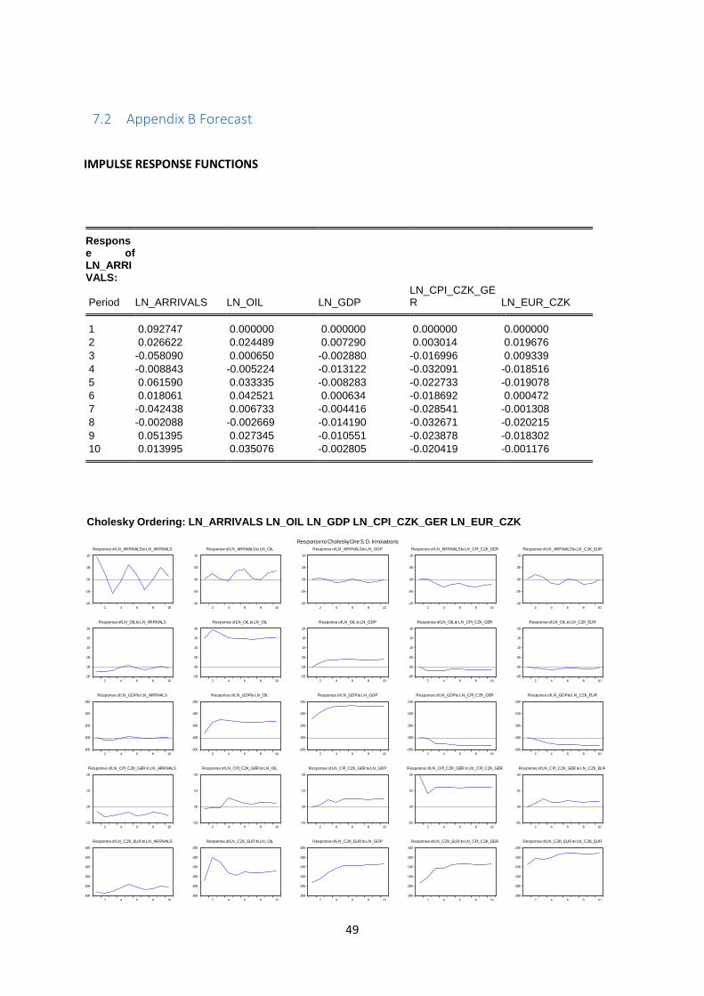
49
7.2 Appendix B Forecast
IMPULSE RESPONSE FUNCTIONS
Response of LN_ARRIVALS:
Period LN_ARRIVALS LN_OIL LN_GDP LN_CPI_CZK_GER LN_EUR_CZK
1 0.092747 0.000000 0.000000 0.000000 0.000000
2 0.026622 0.024489 0.007290 0.003014 0.019676
3 -0.058090 0.000650 -0.002880 -0.016996 0.009339
4 -0.008843 -0.005224 -0.013122 -0.032091 -0.018516
5 0.061590 0.033335 -0.008283 -0.022733 -0.019078
6 0.018061 0.042521 0.000634 -0.018692 0.000472
7 -0.042438 0.006733 -0.004416 -0.028541 -0.001308
8 -0.002088 -0.002669 -0.014190 -0.032671 -0.020215
9 0.051395 0.027345 -0.010551 -0.023878 -0.018302
10 0.013995 0.035076 -0.002805 -0.020419 -0.001176
Cholesky Ordering: LN_ARRIVALS LN_OIL LN_GDP LN_CPI_CZK_GER LN_EUR_CZK
-.10
-.05
.00
.05
.10
2 4 6 8 10
Response of LN_ARRIVALS to LN_ARRIVALS
-.10
-.05
.00
.05
.10
2 4 6 8 10
Response of LN_ARRIVALS to LN_OIL
-.10
-.05
.00
.05
.10
2 4 6 8 10
Response of LN_ARRIVALS to LN_GDP
-.10
-.05
.00
.05
.10
2 4 6 8 10
Response of LN_ARRIVALS to LN_CPI_CZK_GER
-.10
-.05
.00
.05
.10
2 4 6 8 10
Response of LN_ARRIVALS to LN_CZK_EUR
-.05
.00
.05
.10
.15
.20
2 4 6 8 10
Response of LN_OIL to LN_ARRIVALS
-.05
.00
.05
.10
.15
.20
2 4 6 8 10
Response of LN_OIL to LN_OIL
-.05
.00
.05
.10
.15
.20
2 4 6 8 10
Response of LN_OIL to LN_GDP
-.05
.00
.05
.10
.15
.20
2 4 6 8 10
Response of LN_OIL to LN_CPI_CZK_GER
-.05
.00
.05
.10
.15
.20
2 4 6 8 10
Response of LN_OIL to LN_CZK_EUR
-.005
.000
.005
.010
.015
2 4 6 8 10
Response of LN_GDP to LN_ARRIVALS
-.005
.000
.005
.010
.015
2 4 6 8 10
Response of LN_GDP to LN_OIL
-.005
.000
.005
.010
.015
2 4 6 8 10
Response of LN_GDP to LN_GDP
-.005
.000
.005
.010
.015
2 4 6 8 10
Response of LN_GDP to LN_CPI_CZK_GER
-.005
.000
.005
.010
.015
2 4 6 8 10
Response of LN_GDP to LN_CZK_EUR
-.01
.00
.01
.02
2 4 6 8 10
Response of LN_CPI_CZK_GER to LN_ARRIVALS
-.01
.00
.01
.02
2 4 6 8 10
Response of LN_CPI_CZK_GER to LN_OIL
-.01
.00
.01
.02
2 4 6 8 10
Response of LN_CPI_CZK_GER to LN_GDP
-.01
.00
.01
.02
2 4 6 8 10
Response of LN_CPI_CZK_GER to LN_CPI_CZK_GER
-.01
.00
.01
.02
2 4 6 8 10
Response of LN_CPI_CZK_GER to LN_CZK_EUR
.000
.005
.010
.015
.020
.025
2 4 6 8 10
Response of LN_CZK_EUR to LN_ARRIVALS
.000
.005
.010
.015
.020
.025
2 4 6 8 10
Response of LN_CZK_EUR to LN_OIL
.000
.005
.010
.015
.020
.025
2 4 6 8 10
Response of LN_CZK_EUR to LN_GDP
.000
.005
.010
.015
.020
.025
2 4 6 8 10
Response of LN_CZK_EUR to LN_CPI_CZK_GER
.000
.005
.010
.015
.020
.025
2 4 6 8 10
Response of LN_CZK_EUR to LN_CZK_EUR
Response to Cholesky One S.D. Innovations
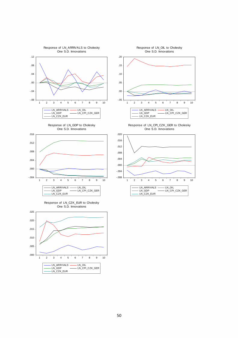
50
-.08
-.04
.00
.04
.08
.12
1 2 3 4 5 6 7 8 9 10
LN_ARRIVALS LN_OIL
LN_GDP LN_CPI_CZK_GER
LN_CZK_EUR
Response of LN_ARRIVALS to Cholesky
One S.D. Innovations
-.05
.00
.05
.10
.15
.20
1 2 3 4 5 6 7 8 9 10
LN_ARRIVALS LN_OIL
LN_GDP LN_CPI_CZK_GER
LN_CZK_EUR
Response of LN_OIL to Cholesky
One S.D. Innovations
-.004
.000
.004
.008
.012
.016
1 2 3 4 5 6 7 8 9 10
LN_ARRIVALS LN_OIL
LN_GDP LN_CPI_CZK_GER
LN_CZK_EUR
Response of LN_GDP to Cholesky
One S.D. Innovations
-.008
-.004
.000
.004
.008
.012
.016
.020
1 2 3 4 5 6 7 8 9 10
LN_ARRIVALS LN_OIL
LN_GDP LN_CPI_CZK_GER
LN_CZK_EUR
Response of LN_CPI_CZK_GER to Cholesky
One S.D. Innovations
.000
.005
.010
.015
.020
.025
1 2 3 4 5 6 7 8 9 10
LN_ARRIVALS LN_OIL
LN_GDP LN_CPI_CZK_GER
LN_CZK_EUR
Response of LN_CZK_EUR to Cholesky
One S.D. Innovations
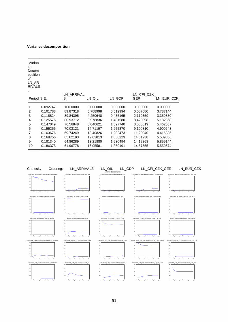
51
Variance decomposition
Variance Decomposition of LN_ARRIVALS:
Period S.E. LN_ARRIVALS LN_OIL LN_GDP
LN_CPI_CZK_GER LN_EUR_CZK
1 0.092747 100.0000 0.000000 0.000000 0.000000 0.000000
2 0.101783 89.87318 5.788998 0.512994 0.087680 3.737144
3 0.118824 89.84395 4.250648 0.435165 2.110359 3.359880
4 0.125576 80.93712 3.978836 1.481580 8.420098 5.182368
5 0.147049 76.56848 8.040621 1.397740 8.530519 5.462637
6 0.155266 70.03121 14.71197 1.255370 9.100810 4.900643
7 0.163676 69.74249 13.40826 1.202473 11.23040 4.416385
8 0.168756 65.62193 12.63813 1.838223 14.31238 5.589336
9 0.181340 64.86289 13.21880 1.930494 14.12868 5.859144
10 0.186378 61.96778 16.05581 1.850191 14.57555 5.550674
Cholesky Ordering: LN_ARRIVALS LN_OIL LN_GDP LN_CPI_CZK_GER LN_EUR_CZK
0
20
40
60
80
100
2 4 6 8 10
Percent LN_ARRIVALS variance due to LN_ARRIVALS
0
20
40
60
80
100
2 4 6 8 10
Percent LN_ARRIVALS variance due to LN_OIL
0
20
40
60
80
100
2 4 6 8 10
Percent LN_ARRIVALS variance due to LN_GDP
0
20
40
60
80
100
2 4 6 8 10
Percent LN_ARRIVALS variance due to LN_CPI_CZK_GER
0
20
40
60
80
100
2 4 6 8 10
Percent LN_ARRIVALS variance due to LN_CZK_EUR
0
20
40
60
80
100
2 4 6 8 10
Percent LN_OIL variance due to LN_ARRIVALS
0
20
40
60
80
100
2 4 6 8 10
Percent LN_OIL variance due to LN_OIL
0
20
40
60
80
100
2 4 6 8 10
Percent LN_OIL variance due to LN_GDP
0
20
40
60
80
100
2 4 6 8 10
Percent LN_OIL variance due to LN_CPI_CZK_GER
0
20
40
60
80
100
2 4 6 8 10
Percent LN_OIL variance due to LN_CZK_EUR
0
20
40
60
80
100
2 4 6 8 10
Percent LN_GDP variance due to LN_ARRIVALS
0
20
40
60
80
100
2 4 6 8 10
Percent LN_GDP variance due to LN_OIL
0
20
40
60
80
100
2 4 6 8 10
Percent LN_GDP variance due to LN_GDP
0
20
40
60
80
100
2 4 6 8 10
Percent LN_GDP variance due to LN_CPI_CZK_GER
0
20
40
60
80
100
2 4 6 8 10
Percent LN_GDP variance due to LN_CZK_EUR
0
20
40
60
80
100
2 4 6 8 10
Percent LN_CPI_CZK_GER variance due to LN_ARRIVALS
0
20
40
60
80
100
2 4 6 8 10
Percent LN_CPI_CZK_GER variance due to LN_OIL
0
20
40
60
80
100
2 4 6 8 10
Percent LN_CPI_CZK_GER variance due to LN_GDP
0
20
40
60
80
100
2 4 6 8 10
Percent LN_CPI_CZK_GER variance due to LN_CPI_CZK_GER
0
20
40
60
80
100
2 4 6 8 10
Percent LN_CPI_CZK_GER variance due to LN_CZK_EUR
0
20
40
60
80
2 4 6 8 10
Percent LN_CZK_EUR variance due to LN_ARRIVALS
0
20
40
60
80
2 4 6 8 10
Percent LN_CZK_EUR variance due to LN_OIL
0
20
40
60
80
2 4 6 8 10
Percent LN_CZK_EUR variance due to LN_GDP
0
20
40
60
80
2 4 6 8 10
Percent LN_CZK_EUR variance due to LN_CPI_CZK_GER
0
20
40
60
80
2 4 6 8 10
Percent LN_CZK_EUR variance due to LN_CZK_EUR
Variance Decomposition
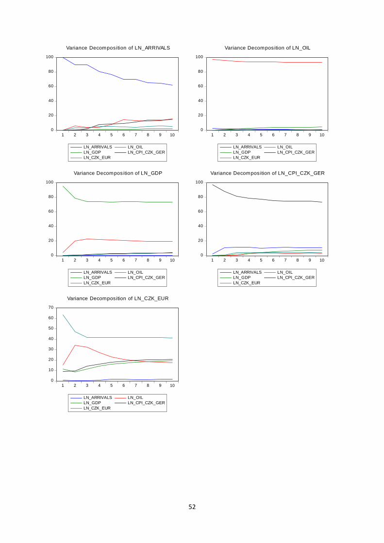
52
0
20
40
60
80
100
1 2 3 4 5 6 7 8 9 10
LN_ARRIVALS LN_OIL
LN_GDP LN_CPI_CZK_GER
LN_CZK_EUR
Variance Decomposition of LN_ARRIVALS
0
20
40
60
80
100
1 2 3 4 5 6 7 8 9 10
LN_ARRIVALS LN_OIL
LN_GDP LN_CPI_CZK_GER
LN_CZK_EUR
Variance Decomposition of LN_OIL
0
20
40
60
80
100
1 2 3 4 5 6 7 8 9 10
LN_ARRIVALS LN_OIL
LN_GDP LN_CPI_CZK_GER
LN_CZK_EUR
Variance Decomposition of LN_GDP
0
20
40
60
80
100
1 2 3 4 5 6 7 8 9 10
LN_ARRIVALS LN_OIL
LN_GDP LN_CPI_CZK_GER
LN_CZK_EUR
Variance Decomposition of LN_CPI_CZK_GER
0
10
20
30
40
50
60
70
1 2 3 4 5 6 7 8 9 10
LN_ARRIVALS LN_OIL
LN_GDP LN_CPI_CZK_GER
LN_CZK_EUR
Variance Decomposition of LN_CZK_EUR
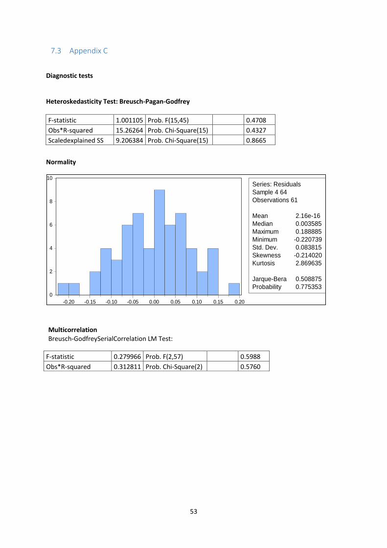
53
7.3 Appendix C
Diagnostic tests
Heteroskedasticity Test: Breusch-Pagan-Godfrey
F-statistic 1.001105 Prob. F(15,45) 0.4708
Obs*R-squared 15.26264 Prob. Chi-Square(15) 0.4327
Scaledexplained SS 9.206384 Prob. Chi-Square(15) 0.8665
Normality
Multicorrelation Breusch-GodfreySerialCorrelation LM Test:
F-statistic 0.279966 Prob. F(2,57) 0.5988
Obs*R-squared 0.312811 Prob. Chi-Square(2) 0.5760
0
2
4
6
8
10
-0.20 -0.15 -0.10 -0.05 0.00 0.05 0.10 0.15 0.20
Series: Residuals
Sample 4 64
Observations 61
Mean 2.16e-16
Median 0.003585
Maximum 0.188885
Minimum -0.220739
Std. Dev. 0.083815
Skewness -0.214020
Kurtosis 2.869635
Jarque-Bera 0.508875
Probability 0.775353