Tecnologias virtuais

Gestão da Água

J. Gomes Ferreira

http://fojo.org/

Universidade Nova de Lisboa

http://gesaq.org/

Lecture outline

• Definitions

• Databases

• Geographic information systems

• Remote sensing

Databases

and GIS

Remote

sensing

Dynamic

models

The Holy Grail

Information

Data

Knowledge

Wisdom

Expensive to acquire

Time

Days Years Decades Centuries

Expensive to process

Soci

etal

inve

stm

ent

Mo

reLe

ssN

on

e

Consolidated experience

Rare and misunderstood

Somewhere between information and knowledge, things start to get useful.

From data to information

• Water quality samples

• Bathymetry

• Remote Sensing

• LiteratureGeoreferenced

Databases

Ecological models

Raw data

GISData-oriented

Processing

Model-orientedProcessing

Management models

Time (years)

Dch

loro

ph

yll

%)

0

2

4

6

8

10

12

14

9 9.1 9.2 9.3 9.4 9.5 9.6 9.7 9.8 9.9 10

Box 23Box 25Box 27Box 30Box 33Box 41

What is virtual technology?

Virtual Technology is defined as any artificial representation of

ecosystems, whether directly (in situ) or indirectly (remote sensing).

Such representations are designed to

help measure, understand, and

predict the underlying variables and

processes.

Simulation of wild species distribution, Loch Creran,

Scotland. (Aquaculture, 274, 313-328)

Distinguish between:

• Tools which allow measurements to be made and translate data

into information (Information and Communication Technology);

• Modelling tools (the way in which information is used for a given

purpose) and the link to data collection technology.

Types of virtual technologyObjective and issues Technology Scale

1 Knowledge

gathering

Database (monitoring, expert

knowledge, literature)

Micro(local) to macroscale

(national, transboundary)

2 Map resources and

environment

GIS, remote sensing Mesoscale (coastal to

national boundaries)

3 Assess system

changes

System approach,

Mathematical models

Meso- (regional) to

macroscale

4 Optimise production Mathematical models Microscale to mesoscale

5 Control production Information technology, sensors Microscale (e.g. aquafarms)

6 Risk assessment Handbooks, models, expert

knowledge, literature, monitoring

Micro to macroscale

(transboundary)

7 Build indicators of

sustainability

Stakeholder forums, enquiries,

indicator databases, LCA

Mesoscale (economic

sector)

8 Communication and

learning

Web technologies, e-learning,

forums, technical networks,

demonstration tools

Meso- (regional) to

macroscale (national,

transboundary)

Data and information

Issue Key variables

Morphology and climate Geometry, bathymetry, rainfall distribution, air

temperature, wind speed, relative humidity

Water availability,

inputs, and exchange

Volume, seasonal and annual hydrographs, tidal

range and prism, current velocities, residence time

Water quality Temperature, salinity, suspended matter, nutrients,

organic detritus, oxygen, chlorophyll, submerged

aquatic vegetation, xenobiotics, microbiology

Environmental

interactions

Fouling, pathogens, extent of submerged aquatic

vegetation, benthos

Thematic data collection for use of virtual tools, applied on scales ranging

from local to watershed.

DatabasesData collection and analysis

Data storage

• Types and volume of data

• Typical storage approaches

• Where do the problems begin?

• How do we move from data to information?

Databases

• What makes a good database?

• Advantages and requirements

• Case studies

Desks do not self-tidy. Data do not self-organize.

DatabasesData types

Raw data

Station name

Station coordinates

(...)

Sample date

Sample time

Sample depth

(...)

Parameter name

Parameter units

(...)

Measured value (result)

(...)

Metadata

Institutions

Teams

Projects

Systems

Campaigns

Products

Formats

Availability

Cost

Data types exhibit wide variation.

DatabasesData volumes

From kilobytes to terabytes

• A typical one-year data collection cycle historically included seasonal

to monthly sampling, a maximum of dozens of stations, some

vertical resolution and a maximum of hundreds of parameters,

particularly if species identification was included

• This typically resulted in 50,000 – 500,000 data items. Tagus (UNDP,

1980s: 68,000 items; Sanggou Bay (INCO, late 1990s): 52,000

items.

• Automated acquisition including moorings and remote sensing have

increased this (already substantial) load by orders of magnitude

• Storage of images and video quickly takes storage to the petabyte

range

The more data there are, the more challenging the storage and retrieval

problem becomes.

Typical storage approaches

• Organized in time: data grouped by date – one set has multiple sampling stations

• Organized spatially: data grouped by location (station) – one set has multiple dates

Data storage in spreadsheets

Station Date Time Depth Secchi Dissolved oxygen Ammonia Chlorophyll

(m) (m) (mg L-1) (umol L-1) (ug L-1)

17 2014.11.11 0900 0.5 1.8 7.3 6.5 2.1

17 2014.11.11 0910 6 - 5.8 8.1 -

17 2014.11.11 0920 11 - 5 8.1 1

56 2014.11.11 1105 0.5 0.7 6.1 15.6 5.6

56 2014.11.11 1115 3 - 5.8 16 5.4

56 2014.11.11 1125 6.5 - 5.8 16.4 5.1

17 2014.11.18 0900 0.5 2.3 - 4.7 2.3

17 2014.11.18 0910 6 - - 4.9 2.1

17 2014.11.18 0920 11 - - 5.6 1.8

56 2014.11.18 1105 0.5 0.9 - 13.4 8.7

56 2014.11.18 1115 3 - - - -

56 2014.11.18 1125 6.5 - - 15.1 8.1

Flatfiles encourage redundancy and empty records—this wastes memory,

lengthens search times, and makes filters difficult.

Database models

• Hierarchical

• Distributed

• Relational

http://www.extropia.com/tutorials/sql/

The relational database model

Data are organized into tables: rows &

columns

Each row represents an instance of an

entity

Each column represents an

attribute of an entity

Metadatadescribe each table column

Relationships between entities are represented by

values stored in the columns of the corresponding tables

(keys)

Accessible through

Standard QueryLanguage (SQL)

•Describes the propertiesor characteristics of otherdata•Does not include sample data•Allows database designers and users to understand the meaning of the data•Takes time to setup

This is one of the most enduring computational models. The internet is

full of examples, and you use them every single day.

RDBMS Advantages

• Controlling redundancy is one of most important feature in DBMS

• Improved data consistency & quality

– Access control

– Transaction control

• Improved accessibility & data sharing

• Increased productivity of application development• Manipulation of the database:

– Retrieval: Querying, generating reports– Modification: Insertions, deletions and updates to its content– Accessing the database through Web applications

• Sharing a database allows multiple users and programs to access thedatabase simultaneously

From Amazon to Expedia, the web has brought RDBS to the masses.

Web databases

• Data are accessible directly through theinternet with integrated DBMS

• Water quality - USGS

• Example of biological databases– WoRMS (http://www.marinespecies.org/)

– Fishbase.org

– http://geo.snirh.pt/snirlit/site/#

• Scientific papers– Web of Knowledge

Water quality of San Francisco Bay, U.S.A.

http://ian.umces.edu/neea/

Agricultural and urban nutrient loading in northern California

Suisun

San Pablo

South Bay

USGS water quality database - San Francisco Bay

Interface is not sexy (pretty much like a decade ago), but the system works.

USGS water quality database - San Francisco Bay

Dataset has no save option, but at least you can copy-paste into Excel.

Web Of Knowledge

RDBMS – Relational Database Management System

Facebook-style RDBMS for storing friends.

Structured Query Language (SQL)

SQL script for generating the Person and Friend tables.

Relational DatabasesEnvironmental management

BarcaWin is an example of a relational database focused on water quality.

The BarcaWin water quality databasewizard for extracting results

Data retrieval usually follows a series of screens or is partly map-based.

Dataset

1. Salinity at different stations and sampling dates

2. River flows, estuary volume3. Tide gauge data

1. Suspended particulate matter2. Primary production rate3. Concentration of N and P4. Nutrient loading5. Bathymetry, tidal prism

Information

1. Estuarine stratification2. Tidal prediction3. Water residence time4. Estuary number

1. Estimated total productivity2.Limiting nutrient for primary production (why is this important?)3. Nutrient removal from system

Data and informationExample for an estuary

Your imagination is the limit in converting data to information—but use

your common sense.

Geographic information systems

GIS is the standard spatial support for water quality analysis.

FOYLE

Bathymetric raster data at25m spatial resolution

Bathymetric data from soundings, coastlineand other contours

Information on:• Sampling stations• Aquaculture sites

BELFAST

CARLINGFORD

STRANGFORD

LARNE

Lough Foyle model box divisionsShellfish density

GIS is used to examine and cross a range of criteria.

CEFAS 2006 survey:Low density of cockles and clams:< 1 ind/m2Very low when compared with cultivated species

Cockles and clams unlikely to pose a serious competition to cultivated species

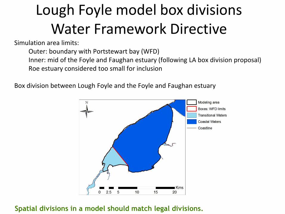
Lough Foyle model box divisionsWater Framework Directive

Spatial divisions in a model should match legal divisions.

Simulation area limits:Outer: boundary with Portstewart bay (WFD)Inner: mid of the Foyle and Faughan estuary (following LA box division proposal)Roe estuary considered too small for inclusion

Box division between Lough Foyle and the Foyle and Faughan estuary

Lough Foyle model box divisionsWater quality criteria

Spatial divisions in a model must take water quality into account.

Respect patterns of nutrient and chlorophyll concentrations

One new division of Lough Foyle: total of 12 boxesDifferentiate between Chl at the NW and NE part of the FoyleNutrients: no new boundaries need to be added

Detail of the Lough Foyle LF11 station from GISShellfish model trial setup at LF11

LF11 was chosen as a trial site for experimental WinShell runs.

Tagus Estuary – Potential locations for oyster culture

Estações

Ostras

3,56 > 0,87 (intertidal)

0,87 > 0 (rarely emersed)

0 > -2 (never emersed)

-2 > -5 -10 > -50

-5 > -10 -50 > -150

Depth (m)

Coordinates

UTM 29 WGS 84

M = 500 000 m

P = 0

¯

Tagus estuary – reclassification based on legislation

Reclassification

F. Vazquez

Unsuitable zones

Suitable zones

(mg L-1

0.9

Zonas Não Adequadas

Chl-a)

T(º C)

10.5

MC

E c

ob

inati

on

5.0

Sal(psu)

Zonas Não Adequadas (Chl-a < 1)

Zonas Adequadas (55 > Chl-a >1)

Re

cla

ssific

ação

Sal(psu)

0.3 31

25

-3.4

1600

305

-2.0

Batimetria(m)

Batimetria(m)

ZonasZNoãonAadsequAaddaes quadas (0,8 < B < 4)

Zonas Adequadas (0.8 < B < 5)

Adequa

+da (30 > T > 10)

T(º C)

14.5 21

18

+

Não Adequado (Sal < 10)

Adequado (40 > Sal > 10)

Reclassificação

Final water quality map

Unsuitable zones

Suitable zones

Tagus estuary - combination of water quality criteria

EcoWin.NET model – TEASMILE

Sample locations, Decorana groupings and sediment types

Benthic species were associated with habitat types, which were used for adding

detailed filtration per box and habitat in EcoWin.

EcoWin.NET model

Shellfish aquaculture management and benthic biodiversity

This approach combines GIS and ecological modelling to assess ecological carrying

capacity.

Sanggou Bay

Xiangshan Gang

Percentage of the system filtered

Wildspecies distribution

Wildspecies filtration

Wildspecies food removalEcosystem food availability

考虑自然条件下的底生多样性的贝类养殖管理

野生种分布

野生种滤食

生态系统可利用的生物量

Review of data available in SMILEBarcaWin search

BarcaWin quickly retrieves thousands of records and saves them to Excel.

• Lough Foyle project database (SMILE) was searched to

extract shellfish growth drivers: temperature, salinity,

chlorophyll, POM, TPM;

• The BarcaWin option ‘show only if all exist’ was used to

obtain a homogeneous dataset;

• The search yielded 289 records, no synoptic ones. Stations

such as LF11 had 4 (incomplete) records;

• The procedure was repeated for the Foyle historical

database (SMILE);

• The search yielded 1280 synoptic records. Station LF11 was

chosen for a trial WinShell model run.

Hunting for shellfish growth drivers

Reworked data for environmental driversShellfish model trial setup at LF11

Data from 1997 (Foyle Historical DB) for WinShell drivers.

Day Temperature Salinity Chlorophyll a POM SPM

ºC psu ug l-1 mg l-1 mg l-1

21 6.3 29.84 0.68 4.5 42.4

70 7.5 30.53 0.47 5.7 21.6

100 9.3 33.54 3 6.65 7.9

107 11.2 31.46 0.54 3.71 20.4

114 9.8 33.9 4.89 7.2 31.04

120 11.1 30 5.76 7.2 28.65

134 10.7 25.6 18.96 9.52 30.48

149 13.8 32.9 2.74 6 29

170 16.3 28.75 1.38 6 25.6

191 16.5 31.53 2.57 6 23.14

205 17 32.13 0.72 8.3 34.8

219 18.7 28.77 0.72 4.8 17.6

233 17.7 33.06 6.4 6 30.8

265 14.2 30.62 3.46 7.2 24

274 13.9 30 2.76 11 38.5

303 9.6 25.41 9.84 10 51

338 6.6 25.68 0.66 4.4 22

WinShell layout for Pacific oyster AquaShell oyster model for Lough Foyle (uncalibrated)

Culture practice data from SMILE.

WinShell mass balance for Pacific oyster AquaShell oyster model for the Foyle

A mass balance analysis helps understand the internal model dynamics.

Remote sensing in coastal zones•Active (provide own energy source) or passive (use available energy)•Data acquisition about an object without touching it (e.g. camera, scanner, radar)•Processing of data•Interpretation of data

Different types of sensors provide data on aquatic systems – freshwater and

estuarine systems are a challenge e.g. due to resolution and interference.

Solar energyReflected (visible) or re-emitted (IR)

Sensor energye.g. Fluorosensor, synthetic aperture radar (SAR)

CZCS derived sea-surface pigments

Mediterranean Sea

Since the construction of the Aswan dam, the eastern Mediterranean has

become increasingly oligotrophic.

5oW 0o 5oE 10oE 15oE 20oE 25oE 30oE 35oE

45oN

40oN

35oN

30oN5oW 0o 5oE 10oE 15oE 20oE 25oE 30oE 35oE

45oN

40oN

35oN

30oN

0.01 0.03 0.05 0.10 0.20 0.30 0.50 1.00 3.00

http://www.obs-vlfr.fr/

Preliminary resource mapping of the Cargados Carajos (St Brandon) Archipelago and Rodrigues byremote sensing using Landsat 7 ETM +, SPOT 4 HRVIR and Aerial photography (E. hardman &O.Tyack. www.bangor.ac.uk)

Classification with ground truthing and habitat mapping in Mauritius

St. Brandon St. Brandon

Rodrigues

Mangrove Degradedmangrove Dwarfmangrove

Bo

er2

00

2.

Wet

lan

ds

Eco

logy

and

M

anag

emen

t,Vo

l.1

0

Pau

la,J

.et

al,1

99

8.

J.P

lan

k.R

es.V

ol2

0

Rem

ote

sen

sin

g cl

assi

fica

tio

n

Rem

ote

sen

sin

gcl

assi

fica

tio

n

Detail for Inhaca Island

Maputo Bay: mangrove habitat classification

1. Dammed fresh water lake.

2. Dammed fresh water lake.

3. Several shrimp ponds.

5. Some pond culture.

6. Bare wetland.

10. Some pond cultures.

11. Fish cages.

12. Reservoir.

13. Some oyster cultures.

Note: Limit inner edge of main culture to -5m isobath.

Sanggou Bay, ChinaRemote sensing for aquaculture

Supervised classification of satellite images

Aquaculture zonation in Sanggou Bay

Landsat image

Kelp structures

Sanggou Bay, ChinaAquatic resources location

AkvaVis – Aquaculture Decision Support

• Applied for mussel and finfish farming

•Three modules share the same

databases but apply information for

different purposes

• Siting module identifies potential farm

sites, simulates carrying capacity

•Management module compiles

information needed by the authorities for

aquaculture management

• Application module promotes efficient

application and ensures that all relevantinformation is provided

WATER - General concept and framework

Thresholds for cultivated species

Thresholds for infrastructure

Environmental datasets

Flight plan

METAMaritime and Environmental

Thresholds

Like any endeavour, ninety percent perspiration, ten percent inspiration.

NETCDFEnvironmental parameter files

META online application

WATER online application

SCI p

ub

sO

nlin

e Exce

l

Des

ign

Imp

ort

RDBMS

Sources

Test

Des

ign

Bu

ild

Web

Test

Analysis and exploitation

META – List thresholds

Online database search to retrieve all thresholds for a species.

WATER – Gilthead in the Greek EEZ

Gilthead suitability shows the best areas are fairly close inshore – the coastal

zone is a complex multi-user seascape.

FARM modelApplication to Integrated Multi-Trophic Aquaculture (IMTA)

Ferreira et al., 2012. Cultivation of gilthead bream in monoculture and integrated multi-trophic aquaculture. Analysis of

production and environmental effects by means of the FARM model. Aquaculture 358-359, p. 23-34.

FARM model for finfish, shellfish, seaweed, and deposit feeders.

Gulf of Guinea – potential for offshore shellfish culture

Cultivation structures are suspended from longlines moored to the bottom.

Gulf of Guinea – Current velocity profiles

Current speed conditions the food supply to bivalves and the dispersal of

finfish waste products.

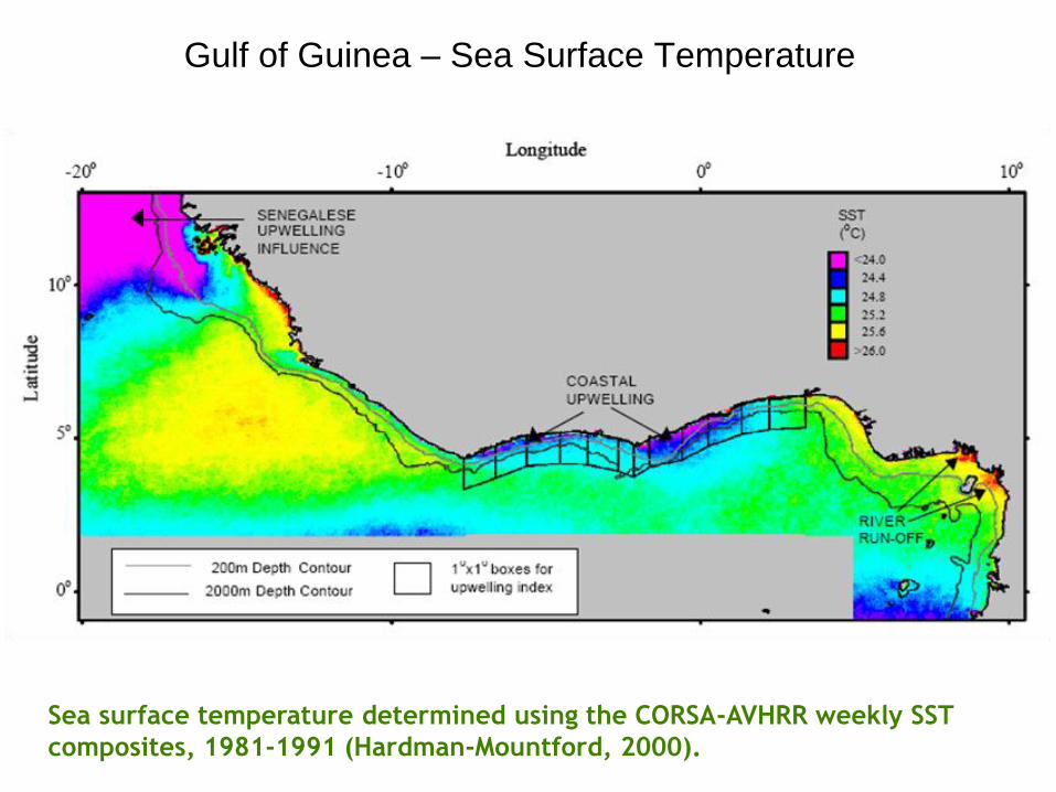
Gulf of Guinea – Sea Surface Temperature

Sea surface temperature determined using the CORSA-AVHRR weekly SST

composites, 1981-1991 (Hardman-Mountford, 2000).

Gulf of Guinea – Remote sensing data for median chlorophyll

An adequate supply of algae is essential for shellfish aquaculture.

Gulf of Guinea – FARM model mass balance for Mediterranean

mussel longline culture (Mytilus galloprovincialis)

About one million dollars annualized revenue, half in products and half in services.

Allochtonous supply of organic material to benthic deposit-feeders below a fish cage

The simplest model with no advection or dispersion considers Ad = Af

Background organics

Sb Sw Sf Sb: Background loading (g d-1)

Sw: Waste feed loading (g d-1)

Sf: Faecal loading (g d-1)

Finfish cage

Sea cucumber pens

Af

Ad

z

Af: Area of polar cage (m2)Ad: Area of benthic footprint (m2)z: Water column depth (m)Zf: fish cage depth

zf

Allochtonous supply of organic material to deposit-feeders under a fish cage

Advection shifts the dispersion footprint as a function of the residual current.

Longitudinal (main) current axis

Polar cage

z

Ad

Mass balance for an Atlantic salmon growth cycle

Matched FCR and end-point weight.

Feed Conversion Ratio (FCR) and mass apportionment Example for 1kg of fish, FCR = 1.12

FCR is the result of input/output. Input-Output = Total Loss

FW to DW conversionConsider a moisture content of 73.65% for Salmo salar muscle (Atanasoff et al., 2013): 1.00 kg wet weight = 0.2635 kg DW.

Feed1120 g DW

Fish intake1033 g DW

Fish mass263.5 g DW

Fish production1000 g WW

Fish faeces177 g DW

Assimilation83%

MetabolismEquiv. 592.5 g DW+ +

Total loss87 g DW

=

FCR1.12

Feed used1033 g DW

• ORGANIX predicts the benthic loading footprint. Many other models (Gowen, Silvert, Cromey, Corner, and respective co-workers) do this;

• Dispersion in 2 dimensions is based on Gaussian distribution functions;

• Advection is based on residual circulation;

• Model algorithm determines time to settle based on fall velocity. Probability distribution (dispersion) and advective shift is determined at each timestep until the plume reaches the bottom;

• Loading from culture structures is distributed over the modelled surface;

• Calibration for Atlantic Salmon, experimental data from DFO and literature. feed pellets fall faster than faeces;

• ORGANIX does not account for physiological variation.

Organic Sedimentation Model - ORGANIX

Calculation of bottom loading and spatial distribution under different culture

and environmental conditions is essential for deposit feeder model.

ORGANIX – ORGANIC Sedimentation model

Multiple deposition plumes of waste feed and faeces for 14 salmon cages

Simulation of sea cucumber growth in integrated culture under salmon farms

0

100

200

300

400

500

600

700

800

900

0 200 400 600 800 1000 1200 1400

Live

Wei

ght

(g)

Days

23 gPOM m-2 d-1

9 gPOM m-2 d-1

5.5 gPOM m-2 d-1

Mass balance for a four year sea cucumber growth cycle

Parastichopus californicus weight data - large animals:100-565 g WW (Hannah et al, 2013),

793-1483 g WW (Hannah et al., 2012).

FARM model – IMTA layout

FARM simulates changes to individual weight, harvest, environment, and income.

200 m

20

0 m 50 m

KelpSalmonOysters

Water flow

Water flow

Fallow

Farm(full view)

Farm

(zo

om

ed v

iew

)

Deposit feeders cover the whole bottom (40,000 m2 per section)

Synthesis of FARM outputs for deposit feedersScenario Mono IMTA 1

5 fish m-2

IMTA 220 fish m-2

IMTA 3Oysters

IMTA 4IMTA 2 + IMTA 3

IMTA 5IMTA4 + seaweeds

Individual weight (g)

112.2 299.8 308.9 128.7 309.1 309.1

Length (cm) 13.5 19.0 19.2 14.2 19.2 19.2

Harvest (t cycle-1)

101.9 581.7 602.6 143.6 603.0 603.0

APP 8.5 48.5 50.2 12.0 50.3 50.3

Profit (k€) as EBITDA

2182 13179 13658 3139 13669 13669

POM removal( gC m-2 y-1)

1043 2437 2518 1191 2520 2520

Net POM loading(g C m-2 y-1)

4 409 5724 5 5874 5874

Population-equivalents (y-1)

5737 13484 13930 7243 14658 18500

Scenarios for monoculture (20 ind. m-2), different finfish densities in IMTA,

shellfish longline culture (100 ind. m-2), shellfish + finfish, and seaweeds (50

ind. m-2). IMTA6 (not shown) increases deposit feeders to 80 ind. m-2.

• Kelp monoculture: final individual weight of 134 g

• Increases to 175 g in IMTA5

• 22% increase in total physical product (TPP) for plants of harvestable size from 153 to 214 t cycle-1

• No significant effect on DIN concentration (P90 decreases by 0.4 mM)

Two key questions

Shellfish suspended culture is not enhanced by salmon culture; seaweeds do

not reduce DIN significantly. This is basin-scale IMTA.

Role of seaweed (winged kelp Alaria esculenta) culture

• Oyster individual weight increases from 60.02 g to 61.65 g

• TPP from 241.9 to 243.9 t cycle-1

• Increase of ratio of suspended particles to 80% makes little difference (end points are 65.7 g and 246.9 t)

Role of suspended shellfish (Pacific oyster C. gigas) culture

Synthesis

• Data per se is of little value

• Models without data are also of little use

• One of the secrets to information is combination

• Social perception themes such as viewsheds from

windparks are now modelled in GIS

• GIS benefits from links to dynamic modelling platforms

• Remote sensing is very useful, and cost-effective, but there

are limitations

• Water quality assessment and management is going

through a technological revolution—and you are part of it

http://gesaq.org/All slides