The INL is a U.S. Department of Energy National Laboratory operated by Battelle Energy Alliance

INL/EXT-16-38751

Revision 0

GETEM User Manual

Gregory L. Mines

July 2016

DISCLAIMER This information was prepared as an account of work sponsored by an

agency of the U.S. Government. Neither the U.S. Government nor any agency thereof, nor any of their employees, makes any warranty, expressed or implied, or assumes any legal liability or responsibility for the accuracy, completeness, or usefulness, of any information, apparatus, product, or process disclosed, or represents that its use would not infringe privately owned rights. References herein to any specific commercial product, process, or service by trade name, trade mark, manufacturer, or otherwise, does not necessarily constitute or imply its endorsement, recommendation, or favoring by the U.S. Government or any agency thereof. The views and opinions of authors expressed herein do not necessarily state or reflect those of the U.S. Government or any agency thereof.

INL/EXT-16-38751

Revision 0

GETEM User Manual

Gregory L. Mines

July 2016

Idaho National Laboratory

Idaho Falls, Idaho 83415

Prepared for the

U.S. Department of Energy

Office of Assistant Secretary for Energy

Efficiency and Renewable Energy (EERE)

Under DOE Idaho Operations Office

Contract DE-AC07-05ID14517

vi

SUMMARY This report provides information for using and understanding the Geothermal Electricity Technology

Evaluation Model (GETEM). GETEM estimates the representative costs associated with generating electrical power from geothermal energy. These projected costs are based upon a number of factors specific to each scenario evaluated; most of these factors are defined by inputs provided. The projected costs and annual power sales can be used to interpret a levelized cost of electricity (LCOE).

The purpose behind GETEM’s development is to allow the U.S. Department of Energy’s Geothermal Technologies Office (GTO) to comply with the Government Performance and Results Act of 1993 (GPRA). GETEM allows GTO to annually assess, quantify, and report the impact of improvements that have occurred with geothermal power generation. In addition, identifying the different contributors to the cost of electricity generated from geothermal energy contributes to GTO understanding of how technology improvements affect generation costs. This assists GTO in developing a research portfolio that provides an optimal return on the investment of taxpayer dollars in its research program. With these goals in mind, INL developed the GETEM model as a series of iterations from 2004 through 2013.

The GETEM User Manual provides a comprehensive overview of this Excel-based model, how to use it, its limitations, and how to interpret the results. It designates the factors that can be inputted manually, as well as those that are automated or fixed. The manual lists and describes available worksheets, their purposes, and how to use them. With the information given, a user can define each facet of a scenario for geothermal energy production, produce useful information for estimating costs, and correctly interpret the results.

Appendices A1–A15 provide more detailed information on aspects of determining power generation costs. These appendices define parameters for scheduling, well count, drilling, and other relevant considerations. They provide sources for pertinent information, such as the U.S. Bureau of Labor Statistics Producer Price Index. They also lay out the mathematical formulas used in the model. Appendix A-14 lists possible errors and warnings that can appear when problematic input is provided, along with helpful explanations of how to resolve them. Appendix A-15 provides information on how to activate the Excel add-ins that are needed to run the program.

Appendices B1 and B2 address resource productivity. They provide valuable information that helps the user understand production issues inherent to geothermal energy production, as well as how they apply to creating estimations in GETEM.

If the instructions in this manual and understood and followed, GETEM can be a highly useful tool for planning and analyzing geothermal energy plants.

vii

ACKNOWLEDGMENT In developing GETEM, multiple individuals from the geothermal industry have provided invaluable input for all phases of the development of a geothermal project. Hopefully the model, as currently configured, adequately depicts that input.

The individuals who have directly contributed to developing the model include: Dan Entingh, Princeton Energy Resources International Gerry Nix and Chad Augustine, National Renewable Energy Laboratory Chip Mansure and John Finger, Sandia National Laboratory Susan Petty, Altarock/Black Mountain Technology Marty Plum, Idaho National Laboratory Mark Paster, Consultant Ella Thodal and Steven Hanson, SRA International Erin Camp, Sentech, Inc. Christopher Richard, BCS, Inc. Ma Seungwook, DOE-EERE Strategic Analysis Group Jay Nathwani, DOE-GTO

In addition, the following Idaho National Laboratory interns have worked to utilize the data reported to the NV DoM to improve GETEM’s characterization of reservoir performance.

Hillary Hanson, University of Idaho Rachel Wood, Washington State University Hannah Wright, Colorado State University Dylan Glenn, Century High School, Pocatello ID

This work was supported by the U.S. Department of Energy, Assistant Secretary for Energy Efficiency and Renewable Energy (EERE), under DOE-NE Idaho Operations Office Contract DE AC07 05ID14517.

viii

CONTENTS

1. Department of Energy’s Geothermal Electricity Technology Evaluation Model (GETEM) ............. 1 1.1 Background .............................................................................................................................. 1 1.2 Model Description .................................................................................................................... 3

1.2.1 Geothermal Project Depiction ..................................................................................... 4 1.2.2 Approach ..................................................................................................................... 5 1.2.3 Model Layout ............................................................................................................ 12 1.2.4 Defining a Scenario for Evaluation ........................................................................... 14

1.3 Model Limitations .................................................................................................................. 34

A1: NET CAPACITY FACTOR ................................................................................................................ 39 Maintenance ..................................................................................................................................... 39

Activities Not Requiring Facility Shutdown .......................................................................... 39 Availability Factor ................................................................................................................. 40 Net Capacity Factor ............................................................................................................... 41

A2: SCHEDULE ......................................................................................................................................... 43

A3: GETEM LCOE CALCULATION ....................................................................................................... 46 Capital Costs ..................................................................................................................................... 46 Depreciation ..................................................................................................................................... 48 Operating and Maintenance (O&M) ................................................................................................. 49 Power Generation ............................................................................................................................. 49 Royalties ........................................................................................................................................... 52 LCOE Determination ........................................................................................................................ 53 Other LCOE Methods ....................................................................................................................... 54

Discounted Cash Flow ........................................................................................................... 54 Fixed Charge Rate .................................................................................................................. 54

A4: LEASING ............................................................................................................................................ 56

A5: WELL COUNT .................................................................................................................................... 58 Hydrothermal Resources .................................................................................................................. 58

Exploration Phase .................................................................................................................. 58 Drilling Phase ......................................................................................................................... 58

EGS Resources ................................................................................................................................. 61 Exploration Phase .................................................................................................................. 61 Drilling Phase ......................................................................................................................... 62

Drilling Before/After PPA ................................................................................................................ 64

A6: DRILLING ........................................................................................................................................... 65 Exploration Drilling: Full-Size Wells............................................................................................... 65 Drilling Phase ................................................................................................................................... 66

Success Rate ........................................................................................................................... 66 Drilling Cost ........................................................................................................................... 67

ix

A7: SURFACE EQUIPMENT.................................................................................................................... 71

A8: GEOTHERMAL PUMPING ............................................................................................................... 73 Approach .......................................................................................................................................... 74

Hydrostatic Pressure .............................................................................................................. 75 Production Well ..................................................................................................................... 76 Injection Well ......................................................................................................................... 79 Reservoir Performance ........................................................................................................... 83 Well Configuration ................................................................................................................ 84 Temperature Loss in Well Bore ............................................................................................. 85

A9: RESERVOIR ....................................................................................................................................... 87 Production Well Flow ....................................................................................................................... 87 Hydraulic Performance ..................................................................................................................... 88 Resource Productivity ...................................................................................................................... 89

Temperature Decline .............................................................................................................. 90 Available Energy .................................................................................................................... 90 Second Law Efficiency .......................................................................................................... 91 Power Output ......................................................................................................................... 93 Makeup Drilling ..................................................................................................................... 94 Application of Approach ........................................................................................................ 95

Makeup Water .................................................................................................................................. 98 Flow in Production and Injection Intervals ...................................................................................... 99

A10: OPERATION AND MAINTENANCE COSTS .............................................................................. 100 Labor 100 Maintenance ................................................................................................................................... 101

Power Plant .......................................................................................................................... 101 Well Field and Gathering System ........................................................................................ 102 Production Pumps ................................................................................................................ 102 Makeup Water ...................................................................................................................... 103 Taxes and Insurance ............................................................................................................. 104 Royalties............................................................................................................................... 104

A11: POWER PLANT .............................................................................................................................. 105 Flash Steam Plants .......................................................................................................................... 105

Flash Conditions .................................................................................................................. 105 Steam Flow .......................................................................................................................... 107 Non-Condensable Gas Removal .......................................................................................... 108 Steam Turbine ...................................................................................................................... 110 Heat Rejection ...................................................................................................................... 111

Plant Size ........................................................................................................................................ 114 Plant Cost ............................................................................................................................. 115

Air-Cooled Binary Plants ............................................................................................................... 121 Binary Plant Component Costs ............................................................................................ 124 Determination of Binary Plant Cost and Performance ......................................................... 131

Transmission Line .......................................................................................................................... 133

x

A12: GEOTHERMAL FLUID PROPERTIES ......................................................................................... 134 General Equations for Saturated Liquid Water .............................................................................. 134 Corrections for Subcooled Water ................................................................................................... 134 Flash Steam Plants .......................................................................................................................... 135 Impact of GETEM Properties on LCOE ........................................................................................ 137 Silica Temperature Limit ................................................................................................................ 137

A13: PRODUCER PRICE INDEXES ...................................................................................................... 140

A14: ERROR AND WARNINGS ............................................................................................................ 142

A15: EXCEL ADD-INS ........................................................................................................................... 146

B1: WELL PRODUCTIVITY .................................................................................................................. 153 Production Well Flow ..................................................................................................................... 153

Flash Plants .......................................................................................................................... 153 Injection Well Flow ............................................................................................................. 156 Supplemental Use of Failed Wells ....................................................................................... 159 Productivity/Injectivity Index .............................................................................................. 161

B2: RESERVOIR PRODUCTIVITY DECLINE: .................................................................................... 163 Binary Plants ........................................................................................................................ 165 Flash Plants .......................................................................................................................... 169

REFERENCES ......................................................................................................................................... 176

FIGURES

Figure 1. GETEM’s characterization of a geothermal project’s development. ............................................ 5

Figure 2. The approach for sizing a project based on level of power sales. ................................................. 6

Figure 3. Capital costs included in GETEM’s determination of an LCOE. .................................................. 8

Figure 4. Down-select process option used by GTO to evaluate impact of exploration R&D on LCOE. ........................................................................................................................................... 9

Figure 5. The approach for estimating capital costs for a binary plant. ...................................................... 10

Figure 6. Screenshot of the Start Here worksheet. ..................................................................................... 15

Figure 7. Screenshot of the Drilling Activities sheet................................................................................... 16

Figure 8. Screenshot of Scenario Definition with two revisions of the default inputs. .............................. 16

Figure 9. Screenshot of the Start Here worksheet after revisions made to the default values. ................... 17

Figure 10. Screenshot of worksheet showing errors and warnings. ............................................................ 18

Figure 11. The Done - Resource Definition button, which is the last step after providing all revisions to GETEM default values (on the Start Here worksheet). .......................................... 18

xi

Figure 12. Screenshot of Start Here worksheet with updated LCOE (after revising default inputs). ........ 19

Figure 13. Estimated power sales for three to five wells with a flow of 90 kg/s (left) and 70 kg/s (right). ......................................................................................................................................... 20

Figure A-1. Snapshot of GETEM’s project activity schedule using default for hydrothermal resource using a binary power plant. .......................................................................................... 44

Figure A-2. Snapshot of GETEM’s project activity schedule with revised input. ...................................... 44

Figure A-3. The effect of temperature decline on power. ........................................................................... 50

Figure A-4. Rate of annual temperature decline that would trigger well field replacement. ...................... 51

Figure A-5. BLM lease sales from June 2007 to September 2014. ............................................................ 56

Figure A-6. The effect of lower drilling rates on well cost based on the SNL models. .............................. 65

Figure A-7. The effect of exploration drilling success rate (50% on left and 60% on right) on GETEM’s effective overall drilling success rate. ....................................................................... 67

Figure A-8. Casing designs for different well depths. ................................................................................ 68

Figure A-9. Summary of drilling costs collected from literature and geothermal industry interviews.................................................................................................................................... 69

Figure A-10. Time variation of the producer price index for drilling oil and gas wells. ............................ 70

Figure A-11. Surface equipment piping system cost estimates. ................................................................. 71

Figure A-12. The impact of production pumping on power sales. ............................................................. 73

Figure A-13. Key parameters used in determining the setting depth for the production pump and the injection pump head. ............................................................................................................. 74

Figure A-14. Effect of binary plant conversion efficiency on calculated geothermal outlet temperatures for both multiple resource temperatures (left) and a 175°C resource (right). ......................................................................................................................................... 82

Figure A-15. Well configurations, with three, four, and five intervals, respectively. ................................ 84

Figure A-16. Estimated temperature loss in the production well. ............................................................... 86

Figure A-17. The effect of a well bore temperature loss on the idea power at 150 and 250°C. ................. 87

Figure A-18. Production well flow rate as it affects plant size and well field size. .................................... 87

Figure A-19. Impact of flow on plant size, well count, and LCOE determined for GTO Hydrothermal C scenario (see Table 1). ..................................................................................... 88

Figure A-20. Effect of hydraulic performance and flow rate on LCOE for the “Hydrothermal C”. .......... 89

Figure A-21. The effect of the decline rate on the produced temperature over time. ................................. 90

Figure A-22. The effect of temperature decline on conversion energy. ..................................................... 93

xii

Figure A-23. The effect of temperature decline rate on both potential to produce power and power. ......................................................................................................................................... 93

Figure A-24. Comparison of estimated and reported power generation at a Nevada binary plant. ............ 96

Figure A-25. Comparison of reported and estimated power generation when including effect of ambient temperatures. ................................................................................................................. 96

Figure A-26. The estimate output versus the reported output at second Nevada binary plant. .................. 97

Figure A-27. Estimated and reported output for Nevada flash plant. ......................................................... 98

Figure A-28. Effect of flashing on amorphous silica solubility temperature. ........................................... 106

Figure A-29. Flash plant process state-points. .......................................................................................... 110

Figure A-30. The relationship between first and second law efficiencies and power produced for a 150°C resource. ........................................................................................................................ 122

Figure A-31. Estimated equipment costs for a 10 MW plant as a function of thermal efficiency (left) and second law efficiency (right). ................................................................................... 122

Figure A-32. Equipment cost estimates for a 100°C (left) and a 200°C resource (right). ........................ 123

Figure A-33. Cost data down select for a 150°C resource. ....................................................................... 124

Figure A-34. GETEM’s minimum equipment cost estimates as functions of second law efficiency for a 150°C resource (a), a 100°C resource (b), and a 200°C resource (c). .............................. 128

Figure A-35. Example of binary plant efficiency producing capital cost minimum for a scenario with fixed power sales (30 MW). ............................................................................................. 131

Figure A-36. Example of binary plant efficiency producing capital cost minimum for a fixed number of production wells (four). ........................................................................................... 132

Figure A-37. Capital cost minimum for a 30 MW air-cooled binary plant (left) and for a similar plant with four wells (right). ..................................................................................................... 132

Figure A-38. Amorphous silica solubility temperatures used in early versions of GETEM. ................... 138

Figure A-39. Current and prior GETEM estimates of amorphous silica solubility temperatures............. 139

Figure A-40. The File tab (top left arrow), Options button (bottom left arrow) and Add-Ins button (right arrow) in Microsoft Excel. .............................................................................................. 146

Figure A-41. The add-ins list in Microsoft Excel. Check this list to see if Solver is active. .................... 147

Figure A-42. The menu for add-ins available in Excel. ............................................................................ 147

Figure A-43. The Developer tab (right arrow) and Visual Basic button (left arrow) in Microsoft Excel. ........................................................................................................................................ 148

Figure A-44. The Tools tab (left arrow) and References option in the Visual Basic menu. ..................... 149

Figure A-45. Box next to Solver option. This should be checked. ........................................................... 149

xiii

Figure B-1. Number of wells and the average flow for each well at Nevada flash plants. ....................... 153

Figure B-2. Distribution of reported flow of Nevada flash plants by decade. .......................................... 154

Figure B-3. Number of production wells and the average flow at Nevada binary plants. ........................ 155

Figure B-4. Distribution of reported flow of Nevada binary plants by decade. ........................................ 156

Figure B-5. The total number of Nevada binary wells with ratio of injection to production wells. ......... 157

Figure B-6. The total number of Nevada flash wells with ratio of injection to production wells. ............ 158

Figure B-7. Reported production and injection flows for Nevada flash wells. ......................................... 159

Figure B-8. Injectivity index and productivity index for Oguni, Sumikawa, Takigami, and Kirishima boreholes with liquid feed zones (Garg 2000). ........................................................ 161

Figure B-9. Injectivity and productivity indices observed during testing of wells in New Zealand. ........ 162

Figure B-10. Effect of declining resource temperature on annual generation for sale. ............................ 164

Figure B-11. Decline of geothermal temperature at Nevada binary plants over a 30-year period............ 165

Figure B-12. Reported wellhead temperature decline over time at Nevada binary facilities. .................. 166

Figure B-13. Temperature decline of the Steamboat Complex over 30 years (left) and as a function of total cumulative production flow (right). ............................................................... 167

Figure B-14. Temperature decline of Nevada binary plants (exclusive of those at the Steamboat Complex) over 30 years. ........................................................................................................... 167

Figure B-15 Temperature decline for newer binary facilities in Nevada. ................................................. 168

Figure B-16. Monthly fluid production and conversion factor between 1986 and 2013 at Beowawe. ................................................................................................................................. 170

Figure B-17. Monthly fluid production and conversion factor between 1988 and 2013 at Dixie Valley........................................................................................................................................ 171

Figure B-18. Estimated geothermal fluid temperature for Dixie Valley based on reported power generation. ................................................................................................................................ 172

Figure B-19. Estimated geothermal fluid temperature for Dixie Valley based on reported power generation when wet bulb temperature exceeded 40°F. ........................................................... 173

Figure B-20. Estimated geothermal fluid temperature at Beowawe based on reported power generation (left) and the same excluding web bulb temperatures of less than 40°F (right). ....................................................................................................................................... 174

TABLES

Table 1. Resource scenarios for assessing impact of technology on generation costs. ................................. 2

xiv

Table 2. GETEM worksheets and their purposes........................................................................................ 13

Table 3. Defaults of the Power Sales input parameter. ............................................................................... 19

Table 4. Defaults of the Economic input parameter. ................................................................................... 21

Table 5. Values for 5-year MACRS depreciation schedule. ....................................................................... 23

Table 6. Defaults of the Permitting input parameter. .................................................................................. 23

Table 7. Defaults of the exploration input parameter. ................................................................................ 24

Table 8. Defaults of the Drilling Activities input parameter. ...................................................................... 26

Table 9. Defaults of the Field Gathering System & Pumping input parameter. ......................................... 29

Table 10. Defaults of the Reservoir Performance input parameter. ........................................................... 30

Table 11. Defaults of the Operations & Maintenance input parameter. ..................................................... 31

Table 12. Defaults of the Power Plant input parameter.............................................................................. 32

Table A-1. Maintenance activities (and related details) that can be done without shutting down a plant. ........................................................................................................................................... 39

Table A-2. Estimated output lost during maintenance activities using the described approach. ................ 40

Table A-3. Results for a 15 MW plant operating with different resource temperatures. ............................ 41

Table A-4. Five-year MACRS depreciation schedule. .............................................................................. 48

Table A-5. Defaults used by GETEM to define well configuration. .......................................................... 85

Table A-6. Hourly rates used to determine labor costs. ............................................................................ 101

Table A-7. Evaporative loss from different geothermal facilities. ............................................................ 112

Table A-8. Constants used in the expressions for different geothermal fluid property estimates. ........... 135

Table A-9. The impact of using GETEM’s correlations for water properties on important project metrics. ..................................................................................................................................... 137

Table A-10. Producer Price Index categories with reference year and description of application to default costs. ............................................................................................................................. 140

Table A-11. Producer Price Indexes by GETEM category, with BLS series ID and description. ............ 141

Table B-1. Summary of flows for Nevada binary and flash plants. .......................................................... 160

Table B-2. Injectivity index values estimated for facilities listed. ............................................................ 162

Table B-3. Decline rates for Dixie Valley and Beowawe. ........................................................................ 174

xv

ACRONYMS BLM Bureau of Land Management

COE cost of electricity

DCF discounted cash flow

DOE Department of Energy

DSR drilling success rate

EERE Office of Energy Efficiency and Renewable Energy

EIA NEMS Energy Information Administration National Energy Modeling System

EPRI Electric Power Research Institute

ESMAP Energy Sector Management Assistance Program (World Bank)

FCR fixed charge rate

GETEM Geothermal Electricity Technology Evaluation Model

GPRA Government Progress and Results Act

GRC Geothermal Resources Council

GTO U.S. Department of Energy’s Geothermal Technologies Office

II Injectivity Index

IPE Icarus Process Evaluator

LCOE levelized cost of electricity

LMTD log mean temperature difference

MACRS modified accelerated cost recovery

MCCA major component cost adjustment

NCF net capacity factor

NCG non-condensable gas

NIST National Institute of Standards of Technology

NV DoM Nevada Division of Minerals

NOAA National Oceanic and Atmospheric Administration

O&G oil and gas

O&M operations and maintenance

PI Productivity Index

PPA power purchase agreement

PPI Producer Price Indexes

ROP rate of penetration (during drilling)

SNL Sandia National Laboratory

SSR stimulation success rate

xvi

WF working fluid

WFPSF working fluid pumps scaling factor

xvii

1

GETEM User Manual 1. Department of Energy’s Geothermal Electricity Technology

Evaluation Model (GETEM) 1.1 Background

The Geothermal Electricity Technology Evaluation Model (GETEM) estimates the representative costs of generating electrical power from geothermal energy. The estimated costs are dependent upon a number of factors specific to the scenario being evaluated, with most of these factors defined by inputs provided. Based on the scenario characterization, cost estimates are developed for all aspects of a project needed to provide the specified or calculated power sales. These costs and annual power sales are the basis for determining a levelized cost of electricity (LCOE).

The driver for GETEM’s development was to allow the U.S. Department of Energy’s Geothermal Technologies Office (GTO) to comply with the Government Performance and Results Act of 1993 (GPRA). GETEM allows GTO to annually assess, quantify, and report the impact of improvements that have occurred with geothermal power generation. In addition, identifying the different contributors to the cost of electricity generated from geothermal energy contributes to GTO understanding of how technology improvements affect generation costs. This assists GTO in developing a research portfolio that provides an optimal return on the investment of taxpayer dollars in its research program.

GETEM was originally developed from 2004 through 2006. A team led by Dan Entingh from Princeton Energy Resources International developed the original model. This team included individuals from industry and the national laboratories who had experience and expertise in different aspects of geothermal project development. At that time, the focus was on developing representative power generation from hydrothermal resources using either flash steam or air-cooled binary conversion systems (plants). For lower-temperature resources, GTO has placed focus on the development of the air-cooled binary technology. Largely because of this emphasis, the binary cycles depicted in GETEM were and continue to be air-cooled.

Initial development efforts ended in 2006, but resumed in 2008 with an emphasis on characterizing generation costs from EGS resources. With resumption of work, all aspects of the model’s development of cost and performance estimates were reviewed and revised where necessary. During this period, the approach for determining generation costs for air-cooled binary plants was modified. The cost and performance of a binary plant is a tradeoff between increasing the amount of power that can be produced from a given geothermal flow rate, and the additional capital costs associated with the more efficient designs. This tradeoff is incorporated into GETEM, in which the impact of performance on both plant costs (which vary directly with performance) and well field costs (which vary indirectly) are considered in establishing the level of performance that minimized the LCOE.

In 2011, GTO revisited the model development in response to industry concerns that its estimates did not adequately reflect the costs to discover a commercially viable hydrothermal resource. From 2011 to 2013, a LCOE analysis team led by Jay Nathwani from GTO conducted a series of interviews with industry subject-area experts to validate both the approaches used in GETEM and the reasonableness of costs that were estimated for the different aspects of project development. Resulting additions and revisions included the following:

• Methods for estimating well costs were revised to reflect the recent well costs provided to the team by Sandia National Laboratory.

• A down-select process was added in which multiple prospects are considered and drilled in order to develop a commercial project.

2

• Power generation costs are now estimated using a discounted cash flow approach developed by the Department of Energy (DOE) for its Office of Energy Efficiency and Renewable Energy (EERE) programs.

The latter two changes allowed GTO to assess the impact of risk of failure in discovering a commercially viable resource. Including the costs incurred at failed prospects increases the costs associated with the exploration phase, while the discounted cash flow methodology allows higher discount rates to be applied to the costs occurring during the early project activities when risk is the greatest. Their effect is to increase the present value of the costs associated with exploration and the contribution of those costs to the project’s LCOE

Prior to this work, GTO did not have specific scenarios defined for assessing the impact of technology on generation costs. As part of the interviews with industry, information was solicited to validate or revise, as necessary, model inputs to account for the variability in resource quality (temperature and productivity) and resource depth. From this information, GTO developed specific EGS and hydrothermal resource scenarios that are the basis for evaluating the impact of recent (for GPRA reporting) and future technology advances on generation costs. The resource scenarios defined are shown in Table 1 below.

Table 1. Resource scenarios for assessing impact of technology on generation costs.

Scenario

Project Life (yr)

Temperature (°C)

Depth (km)

Flow Rate (kg/s)

Production/ Injection

Ratio Plant Type

Power Sales (MW)

EGS A 20 100 2 40 2 to 1 binary 10 EGS B 20 150 2.5 40 2 to 1 binary 15 EGS C 20 175 3 40 2 to 1 binary 20 EGS D 20 250 3.5 40 2 to 1 flash 25 EGS E 20 325 4 40 2 to 1 flash 30 Hydro A 30 140 1.5 100 4 to 3 binary 15 Hydro B 30 175 1.5 80 4 to 3 flash 30 Hydro C 30 175 1.5 100 4 to 3 binary 30 Hydro D 30 225 2.5 80 4 to 3 flash 40 Hydro E 30 140 2.5 100 4 to 3 binary 15

For each resource scenario, the LCOE analysis team developed a unique set of inputs for GETEM.

Subsequent to this work, added emphasis was placed on validating both the model estimates and inputs.

One issue with the earliest versions of the model was the use of fixed values in the calculations that could not be changed and were not always apparent to users. When development work resumed in 2008, these fixed values became model inputs. This practice continued through the work done by the LCOE analysis team. When work by this analysis team was completed, there were ~240 inputs to the model, making GETEM intimidating to use if one lacked sufficient experience and expertise to provide representative inputs for all elements of the geothermal project development.

To facilitate the broader use, default inputs were developed based on the work done by the LCOE analysis team and subsequent validation efforts. At present, GETEM defaults to a specific set of inputs that are based on the specified resource type, temperature, and depth. Of these defaults, 113 can be revised by the user. These inputs were selected for possible revision based on sensitivity analyses done for both EGS and hydrothermal scenarios to identify those inputs having the greatest impact on the LCOE.

3

In 2015, the model’s depiction of project development was aligned with the Geothermal Handbook: Planning and Financing Power Generation, (ESMAP 2012). The modifications did not significantly alter the characterization of the different project activities, but rather changed the timing of the activities (and when their costs are incurred). Obtaining a power purchase agreement (PPA) is now the focal point for depicting the project development and establishing when project costs are incurred.

GETEM is made available to the public with the expectation that any issues with the model’s depiction of a project, or the reasonableness of its estimates, will be conveyed to GTO. While GETEM can be amenable to evaluating a specific project, a user should recognize that the model’s estimates are a representative depiction of a project for the scenario defined. If more than a representative estimate is required for a specific site, those estimates should be made based on the characteristics of that specific site by entities whose business is to perform such evaluations. The values that are provided by GETEM should not be considered or represented as an official DOE estimate of either cost or performance for a specific project.

1.2 Model Description GETEM is an Excel-based tool that estimates the LCOE for a defined geothermal scenario. Only the

generation of electrical power is considered, where the sole source of heat to the power cycle is the geothermal resource. An evaluation is made for either a hydrothermal or an EGS resource, and for either a flash steam or air-cooled binary power plant. GETEM does not evaluate generation costs for water-cooled binary plants or air-cooled flash plants.

With a resource type, temperature, and depth specified, a set of default inputs are established. These inputs, and any revisions made to them, are the basis for the characterization of performance and costs for the different aspects of project development. Two estimates are made: one based on the default inputs (default scenario), and the second based on any revisions made to the default inputs (revised scenario). The only instance when the default scenario changes is if the conversion system is changed from the model default. Costs and performance for both the default and revised scenarios are based on the same resource and conversion system.

Though input can be provided in combinations of SI and Imperial units, calculations are made in Imperial units. Results are provided in Imperial units, though several are given in both sets of units.

All costs are in U.S. dollars. The inputted and calculated costs used to determine the LCOE are “overnight” values; inflation is not incorporated into any of GETEM’s estimates. A discounted cash flow (DCF) methodology is used to determine the LCOE. The present value of costs and revenues are determined at startup using specified discount rates for each phase of the project and a schedule of project activities. Though GETEM retains the fixed charge rate (FCR) methodology initially used to determine generation costs, the LCOE reported by the model is based on the DCF approach.

Each default cost is based upon a specific year, and is adjusted to the year for which the project is being evaluated using a Producer Price Index (PPI) obtained from the Bureau of Labor Statistics (United States Department of Labor). If a default costs is revised, the revision needs to be in the year selected for the scenario evaluation (i.e., PPIs are not applied to revised costs). The PPIs allow projects to be evaluated in prior years (back to 1995) to facilitate evaluation of existing facilities. Though GTO periodically updates the PPIs in GETEM, this may not continue in the future. The specific PPIs from the Bureau of Labor Statistics used are listed in the model (in the Tables worksheet) to facilitate a user’s maintaining the most current values.

The estimates of the LCOE for power generation do not consider incentives that may be available for renewable power generation.

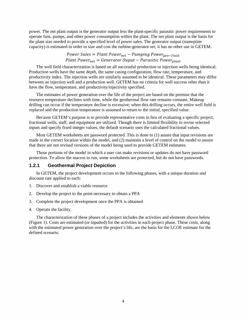
Three levels of power output are used. Power sales are the amount of electricity delivered to the power grid for sale. The magnitude of the power sales is the net plant output less the geothermal pumping

4

power. The net plant output is the generator output less the plant-specific parasitic power requirements to operate fans, pumps, and other power consumption within the plant. The net plant output is the basis for the plant size needed to provide a specified level of power sales. The generator output (nameplate capacity) is estimated in order to size and cost the turbine-generator set; it has no other use in GETEM.

𝑃𝑃𝑃𝑃𝑃𝑃𝑃𝑃𝑃𝑃 𝑆𝑆𝑆𝑆𝑆𝑆𝑃𝑃𝑆𝑆 = 𝑃𝑃𝑆𝑆𝑆𝑆𝑃𝑃𝑃𝑃 𝑃𝑃𝑃𝑃𝑃𝑃𝑃𝑃𝑃𝑃𝑛𝑛𝑛𝑛𝑛𝑛 − 𝑃𝑃𝑃𝑃𝑃𝑃𝑃𝑃𝑃𝑃𝑃𝑃𝑃𝑃 𝑃𝑃𝑃𝑃𝑃𝑃𝑃𝑃𝑃𝑃𝑔𝑔𝑛𝑛𝑔𝑔−𝑓𝑓𝑓𝑓𝑓𝑓𝑓𝑓𝑓𝑓 𝑃𝑃𝑆𝑆𝑆𝑆𝑃𝑃𝑃𝑃 𝑃𝑃𝑃𝑃𝑃𝑃𝑃𝑃𝑃𝑃𝑛𝑛𝑛𝑛𝑛𝑛 = 𝐺𝐺𝑃𝑃𝑃𝑃𝑃𝑃𝑃𝑃𝑆𝑆𝑃𝑃𝑃𝑃𝑃𝑃 𝑂𝑂𝑃𝑃𝑃𝑃𝑃𝑃𝑃𝑃 − 𝑃𝑃𝑆𝑆𝑃𝑃𝑆𝑆𝑆𝑆𝑃𝑃𝑃𝑃𝑃𝑃𝑃𝑃 𝑃𝑃𝑃𝑃𝑃𝑃𝑃𝑃𝑃𝑃𝑝𝑝𝑓𝑓𝑝𝑝𝑛𝑛𝑛𝑛

The well field characterization is based on all successful production or injection wells being identical. Production wells have the same depth, the same casing configuration, flow rate, temperature, and productivity index. The injection wells are similarly assumed to be identical. These parameters may differ between an injection well and a production well. GETEM has no criteria for well success other than it have the flow, temperature, and productivity/injectivity specified.

The estimates of power generation over the life of the project are based on the premise that the resource temperature declines with time, while the geothermal flow rate remains constant. Makeup drilling can occur if the temperature decline is excessive; when this drilling occurs, the entire well field is replaced and the production temperature is assumed to return to the initial, specified value.

Because GETEM’s purpose is to provide representative costs in lieu of evaluating a specific project, fractional wells, staff, and equipment are utilized. Though there is limited flexibility to revise selected inputs and specify fixed integer values, the default scenario uses the calculated fractional values.

Most GETEM worksheets are password protected. This is done to (1) assure that input revisions are made in the correct location within the model, and (2) maintain a level of control on the model to assure that there are not revised versions of the model being used to provide GETEM estimates.

Those portions of the model in which a user can make revisions or updates do not have password protection. To allow the macros to run, some worksheets are protected, but do not have passwords.

1.2.1 Geothermal Project Depiction In GETEM, the project development occurs in the following phases, with a unique duration and

discount rate applied to each:

1. Discover and establish a viable resource

2. Develop the project to the point necessary to obtain a PPA

3. Complete the project development once the PPA is obtained

4. Operate the facility.

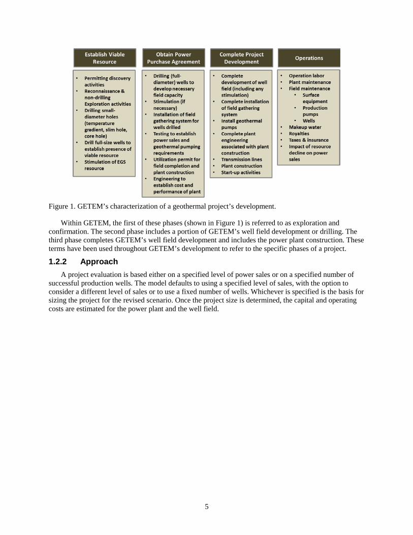
The characterization of these phases of a project includes the activities and elements shown below (Figure 1). Costs are estimated (or inputted) for the activities in each project phase. These costs, along with the estimated power generation over the project’s life, are the basis for the LCOE estimate for the defined scenario.

5

Figure 1. GETEM’s characterization of a geothermal project’s development.

Within GETEM, the first of these phases (shown in Figure 1) is referred to as exploration and confirmation. The second phase includes a portion of GETEM’s well field development or drilling. The third phase completes GETEM’s well field development and includes the power plant construction. These terms have been used throughout GETEM’s development to refer to the specific phases of a project.

1.2.2 Approach A project evaluation is based either on a specified level of power sales or on a specified number of

successful production wells. The model defaults to using a specified level of sales, with the option to consider a different level of sales or to use a fixed number of wells. Whichever is specified is the basis for sizing the project for the revised scenario. Once the project size is determined, the capital and operating costs are estimated for the power plant and the well field.

6

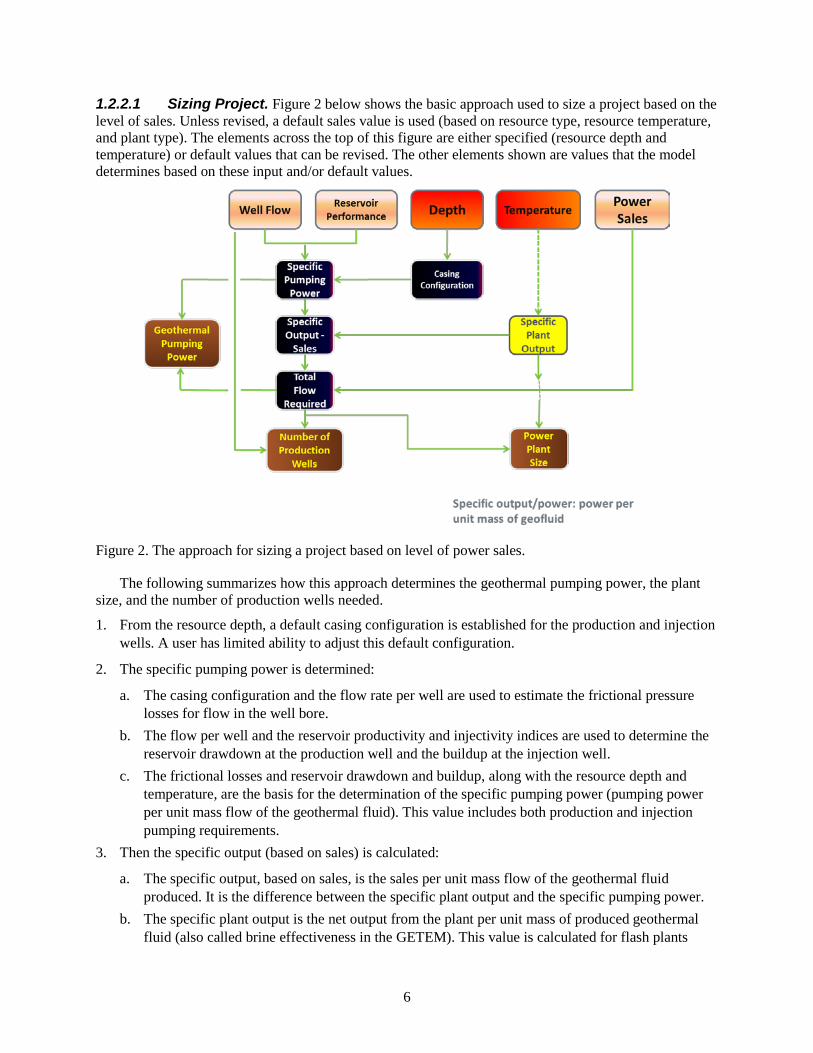
1.2.2.1 Sizing Project. Figure 2 below shows the basic approach used to size a project based on the level of sales. Unless revised, a default sales value is used (based on resource type, resource temperature, and plant type). The elements across the top of this figure are either specified (resource depth and temperature) or default values that can be revised. The other elements shown are values that the model determines based on these input and/or default values.

Figure 2. The approach for sizing a project based on level of power sales.

The following summarizes how this approach determines the geothermal pumping power, the plant size, and the number of production wells needed.

1. From the resource depth, a default casing configuration is established for the production and injection wells. A user has limited ability to adjust this default configuration.

2. The specific pumping power is determined:

a. The casing configuration and the flow rate per well are used to estimate the frictional pressure losses for flow in the well bore.

b. The flow per well and the reservoir productivity and injectivity indices are used to determine the reservoir drawdown at the production well and the buildup at the injection well.

c. The frictional losses and reservoir drawdown and buildup, along with the resource depth and temperature, are the basis for the determination of the specific pumping power (pumping power per unit mass flow of the geothermal fluid). This value includes both production and injection pumping requirements.

3. Then the specific output (based on sales) is calculated:

a. The specific output, based on sales, is the sales per unit mass flow of the geothermal fluid produced. It is the difference between the specific plant output and the specific pumping power.

b. The specific plant output is the net output from the plant per unit mass of produced geothermal fluid (also called brine effectiveness in the GETEM). This value is calculated for flash plants

7

based on flash pressures (established by the resource temperature) and model inputs (default or revised). The specific plant output is the performance metric for the binary plant that is either inputted or determined by GETEM.

c. The specific pumping power is the geothermal pumping power per unit mass of produced flow. It is calculated from the total pumping power determined for a single production and injection well and the flow from an individual production well.

4. The total geothermal flow required is determined from the power sales and the specific output based on sales.

5. The number of successful production wells required is determined from the total geothermal flow rate required and the flow rate per production well.

6. The total geothermal pumping power is determined from the total geothermal flow rate required and the specific pumping power.

7. The power plant size is determined from the total flow rate and the specific plant output.

When the evaluation is based on a fixed number of wells, the total flow is known. That total flow and the specific pumping power are used to determine the total geothermal pumping power. The total flow and the specific plant output establish the power plant output (size). The difference between the plant output and the total geothermal pumping power is the sales that result from the number of production wells specified.

1.2.2.2 Capital Costs. GETEM estimates the capital costs for the following phases of the project development: • Exploration

• Drilling to complete well field

• Field gathering systems for the geofluid

• Power plant construction.

The capital costs that are included in GETEM’s determination of an LCOE are summarized in Figure 3. All costs used to determine the LCOE can be revised by a user, regardless of whether they are default values or calculated by GETEM. A user cannot, however, alter how GETEM estimates costs.

8

Figure 3. Capital costs included in GETEM’s determination of an LCOE.

With the exception of the costs for drilling full-size wells, a contingency is applied to all capital costs in the LCOE determination. The level of contingency applied to the non-drilling costs is an input that can be revised. The correlations used to estimate well costs include a contingency term (which cannot be revised). If a user adjusts the estimates of well costs, the revised value should also include any expected contingency needed for drilling the wells.

Exploration (Discovery):

GETEM assumes that all projects evaluated are Greenfield projects. When a potential resource is discovered, it is not known whether the resource is commercial, and if so, what level of power production can be sustained. As such, the costs determined for this portion of project development are not dependent upon the size of the project.

To find a commercial resource, it may be necessary to evaluate and drill multiple prospects. In order to assess how exploration activities and GTO R&D efforts could impact a project’s LCOE, a down-select process was incorporated into GETEM. This process is depicted below in Figure 4. In order to develop a successful project, multiple sites are initially evaluated, with some of those sites having drilling activities.

9

Figure 4. Down-select process option used by GTO to evaluate impact of exploration R&D on LCOE.

GETEM’s current characterization of the exploration phase includes the upper three activity levels shown in this figure. When this down-select process is used, the capital costs for exploration include those incurred at the unsuccessful sites that are evaluated and drilled, but not developed. If there are multiple unsuccessful sites with drilling, the impact of including their costs on the LCOE can be dramatic. Though the exploration costs for Greenfield resources are not considered a function of the size of the project that is developed, these early project costs will determine the size of a project that is needed in order for the project to be commercially viable.

While the impact of this down-select process on the LCOE can be evaluated, the current default is based only on those costs incurred at the successful site. Costs at this site include those for initial exploration activities, permitting and leasing, drilling of small diameter wells (e.g., slim holes, core holes, and temperature gradient wells), and the drilling and testing of a limited number of full-sized wells to establish that the resource is commercially viable. The LCOE estimate does not include those sites considered but not developed unless the user opts to include the costs incurred at those sites in the revised scenario.

Though it is not the default, GETEM allows for the evaluation of in-field expansion projects as well. If these projects are evaluated, the user will specify those exploration activities to be included in the evaluation.

The costs for the exploration activities are primarily specified inputs; the only calculated cost is that for full-size wells, which is based on the specified resource depth. All default costs can be revised, including the cost of the full-sized wells.

Power Plant and Well Field:

Once the project size is established, capital costs are estimated using the approach depicted below in Figure 5 (for a binary plant). The elements shown on the left side of the figure are the basis for determining the plant and well field capital costs. These values are either inputs or determined when sizing the project.

10

Figure 5. The approach for estimating capital costs for a binary plant.

The binary power plant capital cost is a function of the plant size, the specific plant output, and the resource temperature. Equipment costs are determined as functions of the plant’s second law efficiency, which is determined from the specific plant output and the resource temperature. The equipment costs for the binary plant vary directly with this second law efficiency (i.e., a more efficient power plant is more expensive). The total geothermal flow rate required for the sales varies inversely with the specific plant output (and the second law efficiency). Hence, a more efficient plant may have higher plant equipment costs, but will need less flow, fewer wells, less geothermal pumping power, and a smaller plant size to produce a specified level of sales. A macro in GETEM performs this tradeoff for the binary plants with the specific plant output varied until the LCOE for the specified scenario is minimized.

For the specific output, GETEM determines the cost of the major equipment items and an installation multiplier. This installation multiplier includes both the direct construction costs and the indirect costs, including engineering, home office, and startup. This installation multiplier is applied to the equipment cost estimates to determine the installed cost of the plant needed to provide the sales specified.

With flash plants, costs and performance estimates are based on flash pressures that are either determined by the model or inputted by a user. These pressures, along with estimates of heat rejection and parasitic power requirements, are used to determine the equipment costs. An installation multiplier is applied to the equipment costs to obtain the installed flash plant cost.

This approach for determining installed plant costs by estimating equipment costs and applying an installation multiplier was adopted from Electric Power Research Institute’s Next Generation Geothermal Power Plants study (EPRI 1996). The installation multipliers used are specific to the type of power plant, and are determined using the resource temperature and plant size. This multiplier can be revised.

11

Once the specific power plant output is established, the number of production wells required is determined (see the previous section on sizing a project). The ratio of the production to injection well flow rates, a production well flow rate, and the total flow injected are used to determine the number of injection wells required. From the depth of the well, a well cost is estimated. If the production and injection wells have different depths or casing configurations, their costs will differ. GETEM assumes that all production wells drilled have the same individual cost, regardless of whether or not they are successful. The same assumption applies to all injection wells.

A drilling success rate is used to determine how many wells must be drilled to provide the required number of wells. Unsuccessful wells drilled for a hydrothermal resource can be used to supplement injection. If this option is used, the number of successful injection wells required is decreased, though the number of wells used for injection will increase. This is not an option for EGS resources.

Once the total number of production and injection wells drilled is determined, the individual well cost is multiplied by the total of each type to determine the total production and injection well costs. Their sum is the total drilling cost for the well field. The total well field cost will also include permitting, testing and indirect costs (e.g., engineering, management, and home office).

Note that in the simplified depiction shown in Figure 5, there is no indication of when drilling costs are incurred. GETEM assumes that during the exploration phase for a Greenfield project, one or more full-sized wells that will support power plant operation are drilled. It is also assumed that some portion of the total field capacity must be developed to obtain a PPA; this fraction of capacity needed to obtain the PPA is an input.

Geofluid Field Gathering System:

Costs for the geothermal gathering system are based upon the number of wells being used to support the plant operation. Each well utilized has an associated cost for the surface equipment. This surface equipment cost is determined using an inputted average distance between the plant and well, and an estimated piping size for the specified production well flow rate. This cost per well is multiplied by the number of wells used to determine the total surface equipment cost.

When a binary plant is used, it is assumed that a downhole pump is used with each production well; flash wells default to not using production pumps. The pump setting depth is based on the casing configuration, well flow rate, well depth, fluid temperature, and the productivity index used. This setting depth, well flow rate, and pump efficiency establish the size in horsepower (hp) of the production pump; this size is the basis for the estimated pump cost. The estimated cost does not differentiate between line-shaft and electric submersible pumps. The total cost for production pumps is the product of the estimated pump cost and the number of production wells in service.

An individual injection well is similarly evaluated using the well flow rate, casing configuration, fluid temperature, well depth, and injectivity index to determine the injection well-head pressure needed. This pressure, the total injection flow, and a pump efficiency are used to determine the injection pumping power. Injection pumping is assumed to be provided at a single location using one or more pumps (the model assumes a maximum pump size of 2,000 hp, with more than one pump used if the total power required exceeds this limit). The size (in hp) determined for an individual pump is used to determine the cost of a single pump; the total injection pump cost is the product of the cost of a single pump and the number of injection pumps required.

The cost for the geothermal gathering system is the sum of the surface equipment costs (for both production and injection wells), the total production pump cost, and the total injection pump cost. If spare wells are specified, it is assumed that they will be production wells, and the costs for any production pump and surface piping will be included for each spare well specified. In addition, the total field gathering system includes an indirect cost that is a specified percentage of the total cost.

12

Indirect Costs:

The different phases and activities in project development will have costs that are difficult to categorize and assign a specific value. These costs include planning and management activities, limited testing of exploratory wells, engineering, and other similar expenditures; they also include those costs, exclusive of permitting, associated with obtaining a PPA. Indirect costs are estimated as a percentage of the total cost for the activity or phase. These percentages are specified inputs for each project phase.

1.2.2.3 Operating Costs. The operating costs used in estimating the LCOE include: • Operating labor costs: staffing for plant and well.

• Maintenance costs: a specified fraction of the capital costs for

− the power plant,

− the well field

− the field gathering system.

• Production pump maintenance: the operating life of a production pump, based upon the type of pump specified. Line-shaft pumps are assumed to have a longer operating life, though this pump type also has a cost for the oil (water-soluble) used to lubricate the shaft bearings.

• Makeup water costs: the unit cost for water, which is a function of the resource type and the type of power conversion system utilized, as is the amount of water that must be made up.

• Property taxes and insurance: based upon the total capital cost for the power plant, surface equipment, geothermal pumps, and wells that support the operation of the facility. Exploration costs, aside from the costs of full-size wells supporting plant operation, are not included. Neither are the costs for failed wells not used to operate plant. Any stimulation costs for wells supporting the plant operation are included.

• Royalties: based on the Bureau of Land Management (BLM) royalty schedule.

The inputs used to determine the operations and maintenance (O&M) costs can be revised, or a total O&M LCOE contribution ($ per kW · h) can be specified.

There is further discussion on GETEM’s determination of both capital and operating costs in the Appendices.

1.2.3 Model Layout GETEM contains multiple worksheets in which information is inputted, calculations are made, and

results are presented. The worksheets in the model are described below in Table 2:

13

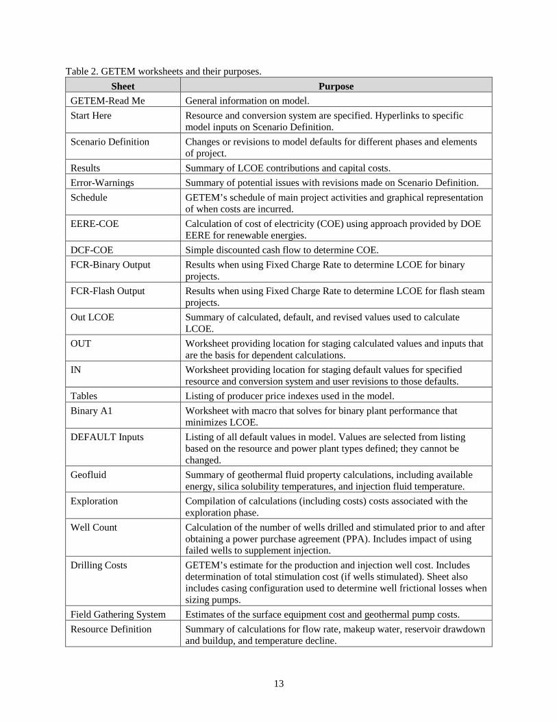
Table 2. GETEM worksheets and their purposes. Sheet Purpose

GETEM-Read Me General information on model. Start Here Resource and conversion system are specified. Hyperlinks to specific

model inputs on Scenario Definition. Scenario Definition Changes or revisions to model defaults for different phases and elements

of project. Results Summary of LCOE contributions and capital costs. Error-Warnings Summary of potential issues with revisions made on Scenario Definition. Schedule GETEM’s schedule of main project activities and graphical representation

of when costs are incurred. EERE-COE Calculation of cost of electricity (COE) using approach provided by DOE

EERE for renewable energies. DCF-COE Simple discounted cash flow to determine COE. FCR-Binary Output Results when using Fixed Charge Rate to determine LCOE for binary

projects. FCR-Flash Output Results when using Fixed Charge Rate to determine LCOE for flash steam

projects. Out LCOE Summary of calculated, default, and revised values used to calculate

LCOE. OUT Worksheet providing location for staging calculated values and inputs that

are the basis for dependent calculations. IN Worksheet providing location for staging default values for specified

resource and conversion system and user revisions to those defaults. Tables Listing of producer price indexes used in the model. Binary A1 Worksheet with macro that solves for binary plant performance that

minimizes LCOE. DEFAULT Inputs Listing of all default values in model. Values are selected from listing

based on the resource and power plant types defined; they cannot be changed.

Geofluid Summary of geothermal fluid property calculations, including available energy, silica solubility temperatures, and injection fluid temperature.

Exploration Compilation of calculations (including costs) costs associated with the exploration phase.

Well Count Calculation of the number of wells drilled and stimulated prior to and after obtaining a power purchase agreement (PPA). Includes impact of using failed wells to supplement injection.

Drilling Costs GETEM’s estimate for the production and injection well cost. Includes determination of total stimulation cost (if wells stimulated). Sheet also includes casing configuration used to determine well frictional losses when sizing pumps.

Field Gathering System Estimates of the surface equipment cost and geothermal pump costs. Resource Definition Summary of calculations for flow rate, makeup water, reservoir drawdown

and buildup, and temperature decline.

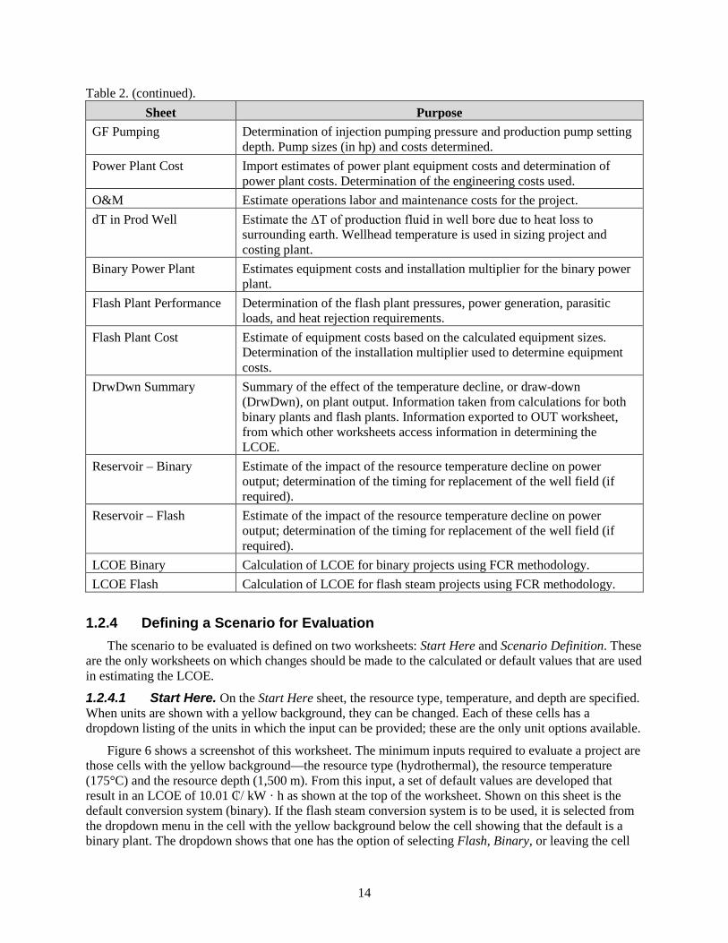
Table 2. (continued).

14

Sheet Purpose GF Pumping Determination of injection pumping pressure and production pump setting

depth. Pump sizes (in hp) and costs determined. Power Plant Cost Import estimates of power plant equipment costs and determination of

power plant costs. Determination of the engineering costs used. O&M Estimate operations labor and maintenance costs for the project. dT in Prod Well Estimate the ΔT of production fluid in well bore due to heat loss to

surrounding earth. Wellhead temperature is used in sizing project and costing plant.

Binary Power Plant Estimates equipment costs and installation multiplier for the binary power plant.

Flash Plant Performance Determination of the flash plant pressures, power generation, parasitic loads, and heat rejection requirements.

Flash Plant Cost Estimate of equipment costs based on the calculated equipment sizes. Determination of the installation multiplier used to determine equipment costs.

DrwDwn Summary Summary of the effect of the temperature decline, or draw-down (DrwDwn), on plant output. Information taken from calculations for both binary plants and flash plants. Information exported to OUT worksheet, from which other worksheets access information in determining the LCOE.

Reservoir – Binary Estimate of the impact of the resource temperature decline on power output; determination of the timing for replacement of the well field (if required).

Reservoir – Flash Estimate of the impact of the resource temperature decline on power output; determination of the timing for replacement of the well field (if required).

LCOE Binary Calculation of LCOE for binary projects using FCR methodology. LCOE Flash Calculation of LCOE for flash steam projects using FCR methodology.

1.2.4 Defining a Scenario for Evaluation The scenario to be evaluated is defined on two worksheets: Start Here and Scenario Definition. These

are the only worksheets on which changes should be made to the calculated or default values that are used in estimating the LCOE.

1.2.4.1 Start Here. On the Start Here sheet, the resource type, temperature, and depth are specified. When units are shown with a yellow background, they can be changed. Each of these cells has a dropdown listing of the units in which the input can be provided; these are the only unit options available.

Figure 6 shows a screenshot of this worksheet. The minimum inputs required to evaluate a project are those cells with the yellow background—the resource type (hydrothermal), the resource temperature (175°C) and the resource depth (1,500 m). From this input, a set of default values are developed that result in an LCOE of 10.01 ₵/ kW · h as shown at the top of the worksheet. Shown on this sheet is the default conversion system (binary). If the flash steam conversion system is to be used, it is selected from the dropdown menu in the cell with the yellow background below the cell showing that the default is a binary plant. The dropdown shows that one has the option of selecting Flash, Binary, or leaving the cell

15

blank. If left blank, the default is used. This default is based on the resource type and the resource temperature. For EGS resources with temperatures of 200°C and lower, a binary plant is the default. If the resource is hydrothermal and the temperature is 200°C or higher, the default is a flash plant. There is an expectation that, with EGS resources, the air-cooled binary plant will be used with higher temperature resources because of the necessity of making up surface water losses. At present, the 200°C limit is approximately the upper limit for production pump technology. This is also the upper resource temperature used in developing the binary plant cost correlations.

Figure 6. Screenshot of the Start Here worksheet.

Just below the LCOE at the top of the page are the power sales for the revised and default scenarios. For this example, the power sales are at the default value of 30 MW. Information and comments are provided in the green font on to the right of the cells where inputs are provided or revised; comments are provided in a similar manner throughout the model. The different project elements shown in red font near the bottom of this screenshot are hyperlinks to the default inputs on the Scenario Definition worksheet. To the right of these links are model results for an important cost or performance value determined using the current input for that portion of the input associated with the hyperlink.

As an example, the input that is being used to develop the indicated cost for drilling can be reviewed by clicking on the Drilling link, which takes one to the inputs for the Drilling Activities, shown below in Figure 7.

16

Figure 7. Screenshot of the Drilling Activities sheet.

Again, comments regarding specific inputs are on the right in the green font. Any revisions to the default values are made in the cells with the yellow background immediately to the left of the defaults. To illustrate how changes are made, consider a scenario in which smaller diameter production wells are used and the flow rate in each successful injection well is twice that of a production well. The input for the production to injection flow ratio is revised to 0.5 and smaller diameter wells are used, as shown below in Figure 8.

Figure 8. Screenshot of Scenario Definition with two revisions of the default inputs.

17

With the change to the production well size, the production well cost is reduced from $2.93M to $2.14M. With the change in the flow to the injection wells, the injection well count is reduced; however, both of these changes increase the amount of geothermal pumping required, resulting in a larger, more expensive plant and increased total brine flow in order to provide the specified power sales. For this scenario, the plant size increased by ~3.8 MW and the number of production wells required increased from 5.77 to 6.40. The higher injection well flow rate decreased the number of injection wells from 3.56 to 2.47. The combined effect was a more expensive project with a higher LCOE.

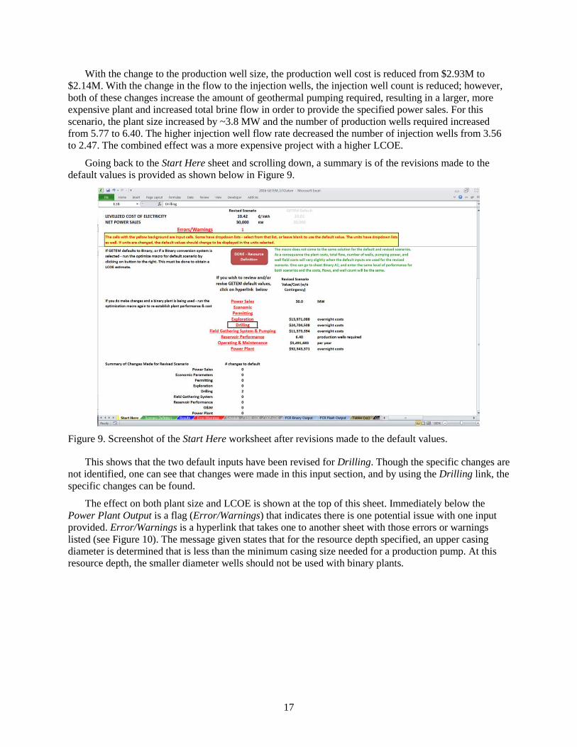
Going back to the Start Here sheet and scrolling down, a summary is of the revisions made to the default values is provided as shown below in Figure 9.

Figure 9. Screenshot of the Start Here worksheet after revisions made to the default values.

This shows that the two default inputs have been revised for Drilling. Though the specific changes are not identified, one can see that changes were made in this input section, and by using the Drilling link, the specific changes can be found.

The effect on both plant size and LCOE is shown at the top of this sheet. Immediately below the Power Plant Output is a flag (Error/Warnings) that indicates there is one potential issue with one input provided. Error/Warnings is a hyperlink that takes one to another sheet with those errors or warnings listed (see Figure 10). The message given states that for the resource depth specified, an upper casing diameter is determined that is less than the minimum casing size needed for a production pump. At this resource depth, the smaller diameter wells should not be used with binary plants.

18

Figure 10. Screenshot of worksheet showing errors and warnings.

To correct any issues or potential issues identified with the inputs provided, hyperlinks are provided to the left of each message. To correct this issue, the link to the Drilling input on the Scenario Definition sheet is selected and the change to the production well size is removed. Returning to the Start Here sheet, the Error/Warning messages have cleared.

When a binary power conversion system is being used, once all changes to the inputs are made, return to the Start Here sheet and click on the Done - Resource Definition button, illustrated in Figure 11. This runs the macro that identifies the level of plant performance that minimizes the LCOE for both the default and revised scenarios.

Figure 11. The Done - Resource Definition button, which is the last step after providing all revisions to GETEM default values (on the Start Here worksheet).

The Start Here sheet after running the macros is shown below in Figure 12

. This shows that, despite the injection wells taking more flow (and presumably decreasing the number of injection wells), the LCOE has increased.

19

Figure 12. Screenshot of Start Here worksheet with updated LCOE (after revising default inputs).

The reasons why the LCOE increased can be found on the summary of the results for both scenarios provided on the Results sheet. The results indicate that with the higher injection well flow rates, the geothermal pumping power increased by ~2MW. To provide the specified 30 MW of sales, a larger power plant is needed, along with more geothermal flow and more required production wells (5.77 to 6.03). As postulated, the number of required injection wells decreased (3.56 to 2.33); however, the combined effect is a higher capital cost and a higher LCOE.

1.2.4.2 Scenario Definition. The default values that can be revised are listed on the Scenario Definition worksheet. They are grouped by the different project elements that are given on the Start Here worksheet. The following discussion reviews default values that can be revised. Power Sales

There are three inputs under Power Sales (shown in Table 3), though only two will be visible to a user at a time.

Table 3. Defaults of the Power Sales input parameter.

Power Sales Input Parameter Hydrothermal

Default EGS Default Comment Is project evaluation based on power sales or production well count? Power Sales Power Sales

Well count refers to number of successful production wells

Power sales binary

T<140°C 140°C<T<175°C T>175°C

10 MW 15 MW 30 MW

10 MW 15 MW 25 MW

flash steam T<250°C T>250°C

30 MW 40 MW

25 MW 30MW

Number of production wells (successful) NA NA Not default

20

Though the temperature ranges and levels of sales are somewhat arbitrary, they are representative of

what one might expect from a resource with three to five producing wells postulated for a Greenfield project. Figure 13 below shows the estimated sales for this number of wells. These estimates are based on the level of performance and flow rate per well taken from the EPRI’s report (EPRI 1996).

Figure 13. Estimated power sales for three to five wells with a flow of 90 kg/s (left) and 70 kg/s (right).

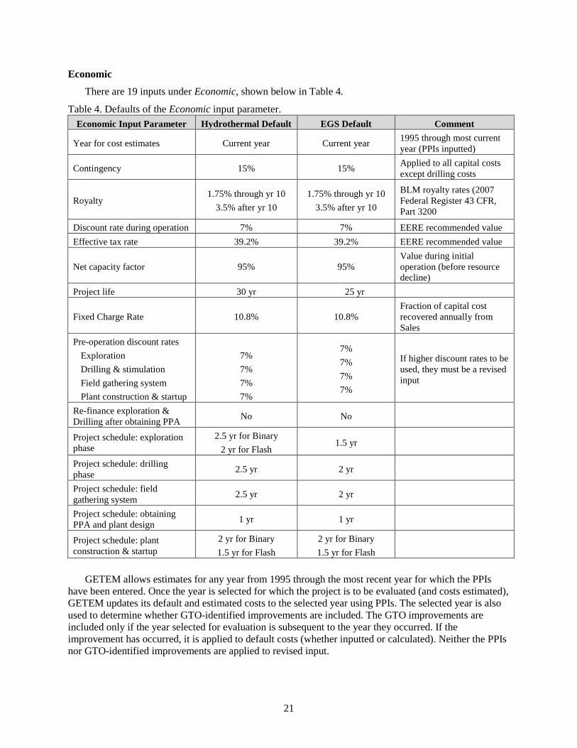
21

Economic

There are 19 inputs under Economic, shown below in Table 4.

Table 4. Defaults of the Economic input parameter. Economic Input Parameter Hydrothermal Default EGS Default Comment

Year for cost estimates Current year Current year 1995 through most current year (PPIs inputted)

Contingency 15% 15% Applied to all capital costs except drilling costs

Royalty 1.75% through yr 10

3.5% after yr 10 1.75% through yr 10

3.5% after yr 10

BLM royalty rates (2007 Federal Register 43 CFR, Part 3200

Discount rate during operation 7% 7% EERE recommended value Effective tax rate 39.2% 39.2% EERE recommended value

Net capacity factor 95% 95% Value during initial operation (before resource decline)

Project life 30 yr 25 yr

Fixed Charge Rate 10.8% 10.8% Fraction of capital cost recovered annually from Sales

Pre-operation discount rates Exploration Drilling & stimulation Field gathering system Plant construction & startup

7% 7% 7% 7%

7% 7% 7% 7%

If higher discount rates to be used, they must be a revised input

Re-finance exploration & Drilling after obtaining PPA No No

Project schedule: exploration phase

2.5 yr for Binary 2 yr for Flash

1.5 yr

Project schedule: drilling phase 2.5 yr 2 yr

Project schedule: field gathering system 2.5 yr 2 yr

Project schedule: obtaining PPA and plant design 1 yr 1 yr

Project schedule: plant construction & startup

2 yr for Binary 1.5 yr for Flash

2 yr for Binary 1.5 yr for Flash

GETEM allows estimates for any year from 1995 through the most recent year for which the PPIs

have been entered. Once the year is selected for which the project is to be evaluated (and costs estimated), GETEM updates its default and estimated costs to the selected year using PPIs. The selected year is also used to determine whether GTO-identified improvements are included. The GTO improvements are included only if the year selected for evaluation is subsequent to the year they occurred. If the improvement has occurred, it is applied to default costs (whether inputted or calculated). Neither the PPIs nor GTO-identified improvements are applied to revised input.

22

Contingency is applied to all capital costs, exclusive of the costs to drill full-sized wells. The level of contingency is not varied between project phases. Any revised costs, excluding wells costs, should be provided without contingency. The default contingency used can be modified. Contingency is not applied to well costs because the correlations used to determine well costs are based on estimates provided by Sandia National Laboratory (SNL) that included contingency. Revisions to these well costs should include contingency.

The default values for both the discount rate during operation and the effective tax rate were provided by the DOE EERE when incorporating the EERE-recommended methodology for estimating LCOE.

The net capacity factor is the ratio of the estimated annual net power generation from the plant relative to the annual generation if the plant had operated continuously at its design net output for the year. The input value used reflects the impact of varying ambient conditions on output, and the lost generation to both maintenance activities and plant outages. It does not include the effect of declining resource productivity—the effect is accounted for elsewhere in GETEM’s calculations. There is further discussion on this metric and the basis for the default value in Appendix A1.

For hydrothermal resources, the project life is based on expected operating life of geothermal plant. There are operating plants in the U.S. with operating lives approaching 30 yrs. The default project life is shorter for EGS resources because of uncertainty in expected reservoir life.

The FCR was used to calculate the LCOE in the original versions of GETEM. Though this method is not used to determine GETEM’s reported generation costs, it has been retained in the model and can be used. The FCR is the fraction of the project capital costs that represents the annual cost for capitalized equipment and services. It includes the rate of return on equity and interest on debt, income taxes, property taxes, and insurance. The default value of 10.8% was the rate that was being used when the FCR methodology was last used by GTO to produce GETEM’s LCOE estimate (in 2012). Inherent to the FCR methodology for LCOE is a fixed project operating life of 30 years.

The LCOE reported in GETEM is determined using a simplified discounted cash flow methodology recommended by the EERE for analysis of renewable energies. This approach allows one to vary the project operating life, and to assign varying discount rates to each of the different phases of project development. For those phases of a project having higher perceived risk, one can apply a higher discount rate to capital costs incurred during that phase. GETEM uses a single default value of 7% for all project phases. This value is consistent with that used in the EERE’s evaluation of other renewables. If these values are revised for the early phases of a project having higher potential risk, there is an option to refinance the costs already incurred, once the PPA is obtained. If this option is selected, the present value of these early costs at the time the PPA is obtained are discounted from that point through startup using the power plant construction discount rate.

The input provided for the duration of the different project phases is used to develop the project schedule. This schedule of project activities and the pre-operation discount rates for the different project phases are used to determine the present value of the pre-operational costs incurred at the start of plant operations. This present value is the basis for the LCOE estimate. There is further discussion as to how this schedule is developed using the input provided (or the default values) in Appendix A2.

The calculation of the LCOE using the discounted cash flow methodology includes a 5-year MACRS (modified accelerated cost recovery) depreciation schedule (Internal Revenue Service 2015). The values used are given below in Table 5.

23

Table 5. Values for 5-year MACRS depreciation schedule. Year Rate

1 205% 2 32% 3 19.25 4 11.52% 5 11.52% 6 5.76%

This deprecation schedule is inherent to the LCOE calculation and cannot be revised. Appendix A3

provides additional discussion as to how GETEM calculates the LCOE.

Permitting

There are five inputs under Permitting, which are given below in Table 6.

Table 6. Defaults of the Permitting input parameter.

Permitting Input Parameter Hydrothermal

Default EGS Default Comment Permitting duration for exploration & early drilling

1 yr prior to 2013 0.5 yr after 2012

1 yr prior to 2013 0.5 yr after 2012

GTO identified improvement in 2013.

Cost to permit pre-drilling exploration activities

$60K prior to 2013

$50K after 2012

$60K prior to 2013

$50K after 2012

Default costs are in 2012 dollars. GTO identified improvement in 2013.

Cost to permit exploration drilling $125K $250K Default costs are in 2012 dollars. Permitting duration for plant and completing well field (utilization permit)

1 yr prior to 2013 0.75 yr after 2012

1 yr prior to 2013 0.75 yr after 2012

GTO identified improvement in 2013.

Cost for utilization permit $1000K $1000K prior

to 2013 $500K after 2012

Default costs are in 2012 dollars. GTO identified improvement in 2013.

The default permitting costs and durations are based on the LCOE analysis team discussions with

industry, which is why default costs are referenced to 2012. GTO has identified improvements that have occurred since 2012—reductions in both the time to permit and the cost to obtain a permit. Those improvements are incorporated into GETEM’s defaults. They are the default values used in the years after GTO identified the improvements; in previous years, the values defined in 2012 are used. Default costs are adjusted to the year evaluated using the PPI for Legal Services.

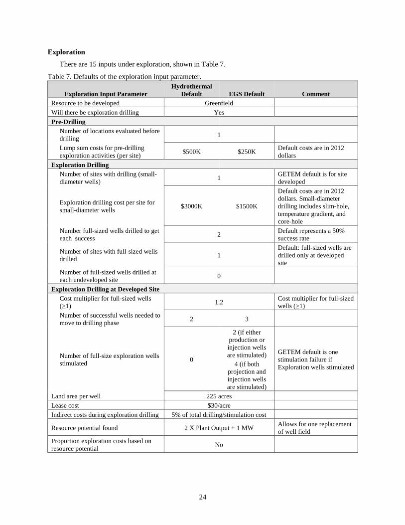
24

Exploration

There are 15 inputs under exploration, shown in Table 7.

Table 7. Defaults of the exploration input parameter.

Exploration Input Parameter Hydrothermal

Default EGS Default Comment Resource to be developed Greenfield Will there be exploration drilling Yes Pre-Drilling

Number of locations evaluated before drilling 1

Lump sum costs for pre-drilling exploration activities (per site) $500K $250K Default costs are in 2012

dollars Exploration Drilling

Number of sites with drilling (small-diameter wells) 1 GETEM default is for site

developed

Exploration drilling cost per site for small-diameter wells $3000K $1500K

Default costs are in 2012 dollars. Small-diameter drilling includes slim-hole, temperature gradient, and core-hole

Number full-sized wells drilled to get each success 2 Default represents a 50%

success rate

Number of sites with full-sized wells drilled 1

Default: full-sized wells are drilled only at developed site

Number of full-sized wells drilled at each undeveloped site 0

Exploration Drilling at Developed Site Cost multiplier for full-sized wells (>1) 1.2 Cost multiplier for full-sized

wells (>1) Number of successful wells needed to move to drilling phase 2 3

Number of full-size exploration wells stimulated 0

2 (if either production or injection wells are stimulated)

4 (if both projection and injection wells are stimulated)

GETEM default is one stimulation failure if Exploration wells stimulated

Land area per well 225 acres Lease cost $30/acre Indirect costs during exploration drilling 5% of total drilling/stimulation cost

Resource potential found 2 X Plant Output + 1 MW Allows for one replacement of well field

Proportion exploration costs based on resource potential No

25

The exploration input has been changed from previous versions of GETEM which allowed a user to provide more detail on the non-drilling activities, as well as the drilling of smaller-diameter wells. This characterization of exploration was modified as part of the updates made by the LCOE analysis team. During the team’s discussions with industry, it was apparent that there was considerable variation in the activities that would occur and what types of wells would be drilled during exploration. Because of this ambiguity, GETEM was revised to characterize both the non-drilling activities and the drilling of small-diameter wells as single lump sum inputs. The default values used for these activities are based on those industry discussions, and are in 2012 dollars (which are adjusted to the year being evaluated using PPIs for Drilling, as well as oil and gas [O&G] support activities).

Though GETEM allows for evaluation using a down-select process, with multiple sites having exploration activities prior to discovery of the site eventually developed, the default considers only those exploration costs incurred at the developed site. When multiple sites with exploration activities are evaluated, the costs incurred at all sites are included in the LCOE determination. Well testing costs for undeveloped sites where full-sized wells are drilled are included; these costs are based on the well test cost specified in the input for drilling phase. Full-sized wells drilled at the undeveloped sites are assumed to have the same cost as the full-sized exploration wells drilled at the developed site.

In aligning GETEM with the Geothermal Handbook (ESMAP 2012), the exploration and confirmation phases in previous versions were combined into a single phase (exploration). With this change, full-size wells are drilled (and for EGS, stimulated) during the exploration phase. The phase now encompasses the discovery of a commercially viable resource. For hydrothermal resources, successful full-size wells drilled during exploration support production for the power plant once operations begin. With EGS resources, the successful wells drilled during exploration include both production and injection wells (default). If two or more wells are successful in this phase, the well type that is stimulated will have one success. If both production and injection wells are stimulated, there will be an equal number of each that are successful.

GETEM does not have an explicit drilling success rate for the exploration phase. Rather, the input asks how many full-sized wells are required to obtain a successful well during this phase. A drilling success rate is the inverse of this value. GETEM’s default is that every other well drilled during exploration is a success (producing a 50% success rate). This default is representative of the early success rates reported in Sanyal’s (2012) summary of worldwide survey of drilling success rates, though it should be noted that there is considerable variation in success rate, especially during the early project drilling.

Further discussion of how GETEM determines the count of full-sized wells in the different project phases is provided in Appendix A5; Appendix A6 provides discussion on drilling success rates.

The default for full-sized wells drilled during the exploration phase is a higher cost than wells drilled when completing the well field. This is consistent with Sanyal’s (2012) paper, which indicated the drilling rate (m/hr) increased as more wells were drilled. The information in this paper was used to estimate the impact of the drilling rate changes on exploration drilling costs. GETEM’s default of a 20% higher drilling cost for full-size wells during exploration are consistent with the estimates made at these lower drilling rates. This evaluation is summarized in Appendix A6.

GETEM estimates the leasing costs based on the inputted cost per acre and estimated acres needed to develop the successful size. It is assumed that the same acreage is required at all sites with drilling activities. The determination of the total leasing costs is summarized in Appendix A4.

The input for resource potential has two uses in GETEM. It determines whether makeup drilling can occur if the resource decline is excessive, and, if so, how many times the well field could be replaced (the GETEM default allows for one replacement). It can also be used in prorating the exploration cost for a project proportionately to the amount of potential used. If this option is used (it is not a default), makeup drilling will not occur to offset the effect of resource decline.

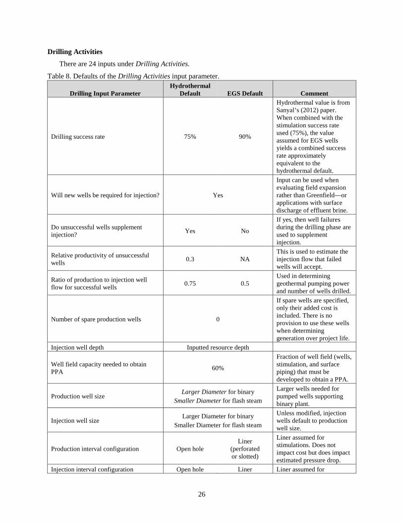
26

Drilling Activities

There are 24 inputs under Drilling Activities.

Table 8. Defaults of the Drilling Activities input parameter.

Drilling Input Parameter Hydrothermal

Default EGS Default Comment

Drilling success rate 75% 90%

Hydrothermal value is from Sanyal’s (2012) paper. When combined with the stimulation success rate used (75%), the value assumed for EGS wells yields a combined success rate approximately equivalent to the hydrothermal default.

Will new wells be required for injection? Yes

Input can be used when evaluating field expansion rather than Greenfield—or applications with surface discharge of effluent brine.

Do unsuccessful wells supplement injection? Yes No

If yes, then well failures during the drilling phase are used to supplement injection.

Relative productivity of unsuccessful wells 0.3 NA

This is used to estimate the injection flow that failed wells will accept.

Ratio of production to injection well flow for successful wells 0.75 0.5

Used in determining geothermal pumping power and number of wells drilled.

Number of spare production wells 0

If spare wells are specified, only their added cost is included. There is no provision to use these wells when determining generation over project life.

Injection well depth Inputted resource depth

Well field capacity needed to obtain PPA 60%

Fraction of well field (wells, stimulation, and surface piping) that must be developed to obtain a PPA.

Production well size Larger Diameter for binary

Smaller Diameter for flash steam

Larger wells needed for pumped wells supporting binary plant.

Injection well size Larger Diameter for binary

Smaller Diameter for flash steam

Unless modified, injection wells default to production well size.

Production interval configuration Open hole Liner

(perforated or slotted)

Liner assumed for stimulations. Does not impact cost but does impact estimated pressure drop.

Injection interval configuration Open hole Liner Liner assumed for

Table 8. (continued).

27

Drilling Input Parameter Hydrothermal

Default EGS Default Comment (perforated or slotted)

stimulations. Does not impact cost but does impact estimated pressure drop.

Production well cost Cost curves (revised for 2015 and later to reflect increased ROP)

If prior to 2015, cost curves based on SNL’s 2010 estimates are used.

Injection well cost Cost curves (revised for 2015 and later to reflect increased ROP)

If prior to 2015, cost curves based on SNL’s 2010 estimates are used.

Are wells stimulated? No Yes

Failed hydrothermal wells can be stimulated. Those wells that fail stimulation cannot be used to supplement production/injection.

Which wells are stimulated? NA Injection wells Option to stimulate injection, production, or both.

Well stimulation cost $2,500K (2012 dollars)

Cost adjusted using PPI for drilling services.

Stimulation success rate 75%

Combined with EGS drilling success rate to produce effective EGS well success approximately equivalent to that used for hydrothermal.

Well testing $150K

(2012 dollars) $500K

(2012 dollars) Postulate longer test for EGS reservoirs.

How are indirect costs determined? % of total costs % of drilling costs 5% Lump sum No

With Greenfield developments, one or more successful full-sized wells are drilled during the

exploration phase. These successful exploration wells contribute to the required production and injection capacity needed for the facility. The remaining well field capacity is developed in the subsequent drilling phase. The input in this section is the basis for determining how many wells must be drilled in this phase and the associated cost.

The drilling success rate represents the fraction of the wells that are drilled that are successful; there is no specified criteria for success other than successful production wells that provide the specified flow, temperature, and productivity; similarly, all successful injection wells will accept the specified flow and have the same injectivity.

The depiction of hydrothermal scenarios has been revised to allow those wells that are not successful to be used to supplement injection. When utilizing failed wells (now a GETEM default), all failed production and injection wells are used. It is assumed that failed wells lack the necessary productivity or injectivity to be successful; the specified relative productivity of the failed well is used to determine injection flow in that well.

28

The flow rate for a successful injection well is based on the specified ratio of flow relative to a successful production well. In prior versions of GETEM, the ratio of injection to production wells was specified. This change accommodates the option to use failed wells to supplement injection.

The current version of GETEM also has an option to not drill new injection capacity. This is for use in field expansion developments for which existing injection capacity is sufficient to support the new expansion. It can also be used to evaluate projects where brine leaving the plant discharges to the surface (no cost is assigned to this type of brine disposal).

The project schedule is now based on when the PPA is obtained, with the premise that to get a PPA, some percentage of the well field capacity must be developed and confirmed. Well testing and associated costs are incurred prior to the PPA. The fraction of the capacity needed for the PPA is used to establish how many successful wells are required (both production and injection). This count of successful wells required establishes how many are drilled (and for EGS, stimulated) prior to the PPA. These total wells drilled establish costs incurred in the Drilling phase prior to and after obtaining the PPA.

A detailed discussion of how GETEM determines the number of wells required and drilled is provided in Appendix A5.

In determining well costs, GETEM utilizes one of two cost correlations depending upon whether the well size is Larger Diameter or Smaller Diameter. The default is to use the larger-diameter well with binary plants that are assumed to require downhole pumps; these pumps provide the necessary flow rates and maintain the geothermal fluid in the liquid phase. The larger-diameter well configuration assures that the upper casing interval in the well will accommodate the pump. Though EGS resources may have lower flow rates, GETEM still defaults to the larger well size with binary plants in order to accommodate the use of production pumps. The current default is to use the smaller-diameter well size for flash plants, with the expectation that they will not use production pumps. The injection well defaults to the default size for the production well.

GETEM also has input for the configuration of the production and injection intervals (i.e., whether they are open hole or used a perforated or slotted liner). This input does not impact the well cost. It is used to estimate the frictional losses in that portion of the well bore; these losses are used in determining both production and injection pumping power.

Appendix A6 provides information on the basis for the well cost estimates.

EGS resources default wells that are stimulated; this cannot be revised. It is probable that there will be a relationship between the stimulation cost and the performance (thermal, hydraulic, and flow) of the EGS reservoir created. At this time, there is insufficient information to characterize this relationship. A fixed value is used for stimulation on the premise that it will be sufficient to provide the reservoir and well performance specified. The current default used resulted from the LCOE analysis team discussions with industry with respect to a potential stimulation cost.

Similarly, there is insufficient information available to establish values for the success in developing a successful EGS well. The approach assumes a successful EGS well requires both successful drilling and successful stimulation. Current defaults assume that the success rate in drilling an EGS well will be high, with a lower rate for successful stimulation. The combined success rate is approximately equivalent to the default for a successful hydrothermal well, with the expectation that as the technology and expertise develop, the success rate for stimulation will increase.

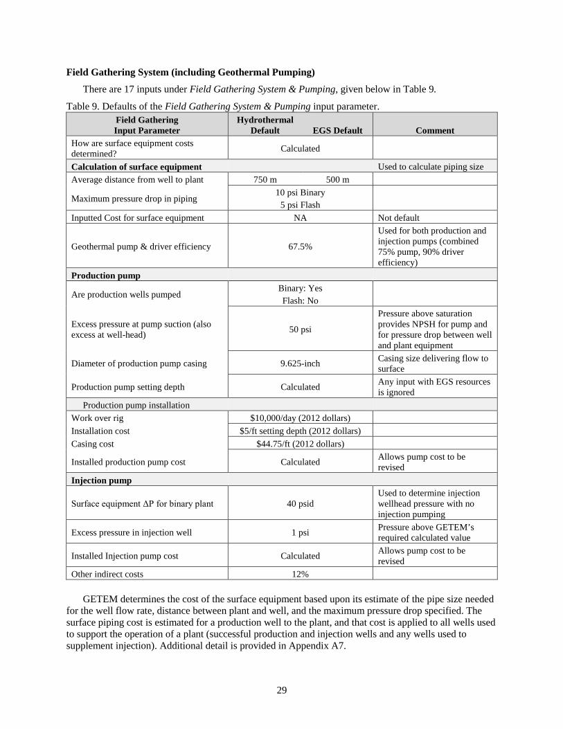
29

Field Gathering System (including Geothermal Pumping)

There are 17 inputs under Field Gathering System & Pumping, given below in Table 9.

Table 9. Defaults of the Field Gathering System & Pumping input parameter. Field Gathering Input Parameter

Hydrothermal Default EGS Default Comment

How are surface equipment costs determined? Calculated

Calculation of surface equipment Used to calculate piping size Average distance from well to plant 750 m 500 m

Maximum pressure drop in piping 10 psi Binary

5 psi Flash

Inputted Cost for surface equipment NA Not default

Geothermal pump & driver efficiency 67.5%

Used for both production and injection pumps (combined 75% pump, 90% driver efficiency)

Production pump

Are production wells pumped Binary: Yes Flash: No

Excess pressure at pump suction (also excess at well-head) 50 psi

Pressure above saturation provides NPSH for pump and for pressure drop between well and plant equipment

Diameter of production pump casing 9.625-inch Casing size delivering flow to surface

Production pump setting depth Calculated Any input with EGS resources is ignored

Production pump installation Work over rig $10,000/day (2012 dollars) Installation cost $5/ft setting depth (2012 dollars) Casing cost $44.75/ft (2012 dollars)

Installed production pump cost Calculated Allows pump cost to be revised

Injection pump

Surface equipment ΔP for binary plant 40 psid Used to determine injection wellhead pressure with no injection pumping

Excess pressure in injection well 1 psi Pressure above GETEM’s required calculated value

Installed Injection pump cost Calculated Allows pump cost to be revised

Other indirect costs 12%

GETEM determines the cost of the surface equipment based upon its estimate of the pipe size needed for the well flow rate, distance between plant and well, and the maximum pressure drop specified. The surface piping cost is estimated for a production well to the plant, and that cost is applied to all wells used to support the operation of a plant (successful production and injection wells and any wells used to supplement injection). Additional detail is provided in Appendix A7.

30

Estimates of the geothermal pumping power required are based upon the well depth, the well casing configuration, and the reservoir parameters defined (flow and either productivity or injectivity index.) Pump costs are based upon the horsepower requirements determined. The methodology used in determining the required pumping power; the cost for that pumping is provided in Appendix A8.

Reservoir Performance

There are nine inputs under Reservoir Performance, which are listed below in Table 10.

Table 10. Defaults of the Reservoir Performance input parameter. Reservoir Performance Input

Parameter Hydrothermal

Default EGS Default Comment

Production well flow rate Binary: 110 kg/s

Flash: 80 kg/s

Binary and Flash: 40 kg/s

Lower flow for EGS represents current performance of EGS reservoirs (data very limited).

Hydraulic Performance of Reservoir

Productivity index Binary 2,500 lb/hr per psi Flash 2,500 lb/hr per psi

Value used in EPRI’s Next Generation Geothermal Power Plants study (EPRI 1996). Same values used for both hydrothermal and EGS.

Injectivity index Same as Productivity Index default Thermal Drawdown

Annual temperature decline rate Binary 0.5% Flash 0.6%

Binary 0.5% Flash 0.5%

Value impacts the amount of power produced over the life of the plant.

Maximum temperature decline allowed Value calculated; corresponds to ~

10% decline in the Carnot efficiency

Triggers the replacement of the well field (if there is sufficient resource potential).

Makeup Water

Makeup water losses from flash steam plant No Yes

Assume that all water losses must be replaced when using an EGS resource.

EGS subsurface water losses NA 5% of injected flow

Assume that some portion of the injected fluid is not produced with EGS resources.

Makeup water cost $300/acre-ft

Binary $300/acre-ft

Flash $2,000/acre-ft

EGS flash has a higher cost because it is assumed that a higher quality of water will be needed. If quality of water used to replace steam condensate lost is low, the salinity of the produced fluid will increase over time.

Flow into/out of multiple zones in production/injection interval No Yes

This calculates the frictional losses in the production and injection intervals assuming that the flow enters or exits along the entire length of the interval.

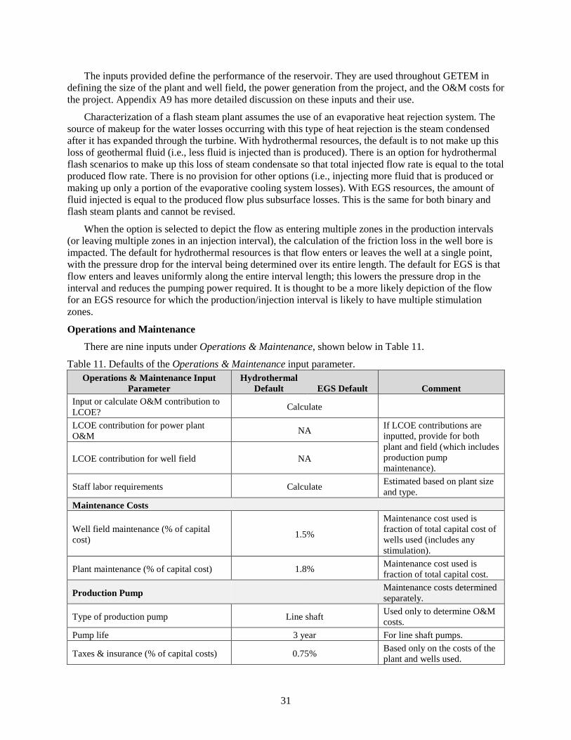
31

The inputs provided define the performance of the reservoir. They are used throughout GETEM in defining the size of the plant and well field, the power generation from the project, and the O&M costs for the project. Appendix A9 has more detailed discussion on these inputs and their use.

Characterization of a flash steam plant assumes the use of an evaporative heat rejection system. The source of makeup for the water losses occurring with this type of heat rejection is the steam condensed after it has expanded through the turbine. With hydrothermal resources, the default is to not make up this loss of geothermal fluid (i.e., less fluid is injected than is produced). There is an option for hydrothermal flash scenarios to make up this loss of steam condensate so that total injected flow rate is equal to the total produced flow rate. There is no provision for other options (i.e., injecting more fluid that is produced or making up only a portion of the evaporative cooling system losses). With EGS resources, the amount of fluid injected is equal to the produced flow plus subsurface losses. This is the same for both binary and flash steam plants and cannot be revised.

When the option is selected to depict the flow as entering multiple zones in the production intervals (or leaving multiple zones in an injection interval), the calculation of the friction loss in the well bore is impacted. The default for hydrothermal resources is that flow enters or leaves the well at a single point, with the pressure drop for the interval being determined over its entire length. The default for EGS is that flow enters and leaves uniformly along the entire interval length; this lowers the pressure drop in the interval and reduces the pumping power required. It is thought to be a more likely depiction of the flow for an EGS resource for which the production/injection interval is likely to have multiple stimulation zones.

Operations and Maintenance

There are nine inputs under Operations & Maintenance, shown below in Table 11.

Table 11. Defaults of the Operations & Maintenance input parameter. Operations & Maintenance Input

Parameter Hydrothermal

Default EGS Default Comment Input or calculate O&M contribution to LCOE? Calculate

LCOE contribution for power plant O&M NA If LCOE contributions are

inputted, provide for both plant and field (which includes production pump maintenance).

LCOE contribution for well field NA

Staff labor requirements Calculate Estimated based on plant size and type.

Maintenance Costs

Well field maintenance (% of capital cost) 1.5%

Maintenance cost used is fraction of total capital cost of wells used (includes any stimulation).

Plant maintenance (% of capital cost) 1.8% Maintenance cost used is fraction of total capital cost.

Production Pump Maintenance costs determined separately.

Type of production pump Line shaft Used only to determine O&M costs.

Pump life 3 year For line shaft pumps.

Taxes & insurance (% of capital costs) 0.75% Based only on the costs of the plant and wells used.

32

GETEM has an option to use inputted values for the O&M contribution to the LCOE. When this

option is used, a contribution is provided for both the power plant and the well field. Both inputs are to include any chemical costs associated with the plant and field operation. The inputted field cost contribution is to include the cost for maintenance of the production pumps as well as taxes and insurance. If there are royalties (an input), they are determined separately and added to the inputted value in defining the total O&M contribution for the project.

The labor staff for the project includes staff for the operation of both the plant and well field. The default value used is determined from the plant type and size. When modular units are used, the default uses additional staff.

Annual maintenance costs for the field and plant are determined as a fraction of the initial capital cost. The field maintenance is based on the capital cost of those wells used to support operation of the plant. If the wells were stimulated, those costs are included in the field capital cost used. The field gathering system costs, exclusive of the production pumps, are also included in the field capital costs used to determine the annual maintenance costs for the well field.

The annual maintenance cost contribution for production pumps is determined separately. The type of production pump specified is used to determine the associated maintenance and pump life; the pump type is not used in estimating the capital costs of these pumps.

Annual taxes and insurance are based on the capital costs of all equipment and wells that support the operation of the plant. These are property taxes, not taxes on sales revenues (see Appendix A3 for discussion on the inclusion of tax on sales revenues in the determination of the LCOE).

Specifics on the determination of the O&M costs are provided in Appendix A10.

Power Plant

There are 17 inputs under Power Plant, shown below in Table 12.

Table 12. Defaults of the Power Plant input parameter.

Power Plant Input Parameter Hydrothermal

Default EGS Default Comment Transmission Line Cost

Are transmission line costs included? No GTO does not include transmission costs when assessing LCOE.

Length of transmission line 0 No transmission line costs are included.

Transmission line cost $0 No transmission line costs are included.

Plant

Indirect plant construction costs 12% of direct construction costs For engineering, home office, and startup.

Binary Number of binary modular units used to provide specified sales 1

Performance metric brine effectiveness Calculated Calculated value minimizes LCOE.

Direct construction multiplier Calculated Applied to major component costs to determine the direct construction cost.

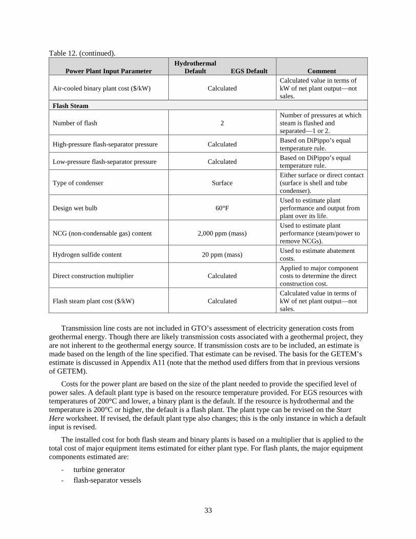
Table 12. (continued).

33

Power Plant Input Parameter Hydrothermal

Default EGS Default Comment

Air-cooled binary plant cost ($/kW) Calculated Calculated value in terms of kW of net plant output—not sales.

Flash Steam

Number of flash 2 Number of pressures at which steam is flashed and separated—1 or 2.

High-pressure flash-separator pressure Calculated Based on DiPippo’s equal temperature rule.

Low-pressure flash-separator pressure Calculated Based on DiPippo’s equal temperature rule.

Type of condenser Surface Either surface or direct contact (surface is shell and tube condenser).

Design wet bulb 60°F Used to estimate plant performance and output from plant over its life.

NCG (non-condensable gas) content 2,000 ppm (mass) Used to estimate plant performance (steam/power to remove NCGs).

Hydrogen sulfide content 20 ppm (mass) Used to estimate abatement costs.

Direct construction multiplier Calculated Applied to major component costs to determine the direct construction cost.

Flash steam plant cost ($/kW) Calculated Calculated value in terms of kW of net plant output—not sales.

Transmission line costs are not included in GTO’s assessment of electricity generation costs from

geothermal energy. Though there are likely transmission costs associated with a geothermal project, they are not inherent to the geothermal energy source. If transmission costs are to be included, an estimate is made based on the length of the line specified. That estimate can be revised. The basis for the GETEM’s estimate is discussed in Appendix A11 (note that the method used differs from that in previous versions of GETEM).

Costs for the power plant are based on the size of the plant needed to provide the specified level of power sales. A default plant type is based on the resource temperature provided. For EGS resources with temperatures of 200°C and lower, a binary plant is the default. If the resource is hydrothermal and the temperature is 200°C or higher, the default is a flash plant. The plant type can be revised on the Start Here worksheet. If revised, the default plant type also changes; this is the only instance in which a default input is revised.

The installed cost for both flash steam and binary plants is based on a multiplier that is applied to the total cost of major equipment items estimated for either plant type. For flash plants, the major equipment components estimated are:

- turbine generator - flash-separator vessels

34

- cooling tower - condenser - pumps - non-condensable gas removal system - hydrogen sulfide abatement system

For binary plants, the major equipment components estimated are

- turbine generator - air-cooled condenser - geothermal heat exchangers - working fluid pump The direct construction multiplier for each plant type includes all materials and remaining equipment,

labor and supervision, taxes, and freight. A second multiplier is also applied for the indirect costs associated with the plant installation. These indirect costs include home office, engineering, and plant startup costs. The approach used is analogous to that used in EPRI’s report (EPRI 1996).

Flash steam plant performance and cost are determined using the specified inputs.

The binary plant performance metric is the brine effectiveness, or net plant output, per unit mass flow of geothermal fluid. Along with the resource temperature and plant size, this metric is used to determine the binary plant cost. Because this metric affects the amount of geothermal fluid required, it also impacts the number of wells required, the field gathering system cost, and the geothermal pumping power. GETEM includes a macro that varies the brine effectiveness until a LCOE minimum is obtained. If a value is specified for this metric, the macro does not affect the revised scenario LCOE. The macro can be run from the Start Here or Binary A1 worksheets.

The reported costs are in $/kWnet, with the net power being the net output from the plant—not power sales. If calculated values for plant cost are revised, the input should also be provided in terms of net plant output.

There is further discussion on GETEM’s calculations of both performance and cost for both the flash steam and binary plants provided in Appendix A12.

1.2.4.3 Default Inputs. The default inputs used in GETEM cannot be revised by a public user. The values used for defaults are provided on the Default Inputs worksheet. Only GTO can revise these default values on this sheet. Selected defaults can be revised on the Scenario Definition worksheet. Those values that can be revised were found to have the larger impacts on the LCOE when considering a probable range of values for the input parameter.

1.3 Model Limitations GETEM is intended to provide representative generation costs from geothermal energy. While it is

amenable to examining costs at specific sites, its estimates are indicative of what costs and performance could be. If costs and performance are needed beyond a preliminary assessment, those estimates should be provided by an industry professional.

Estimates are indicative of what could be done with current technology. If one desires to know the impact of a new technology on LCOE, it is necessary that the impact be quantified in terms of how it will impact cost and performance. If GETEM’s inputs do not reflect either cost or performance metrics determined, the technology impact cannot be evaluated.

PPIs from the Bureau of Labor Statistics are used to bring model estimates from the year for which they are based to the specified year for evaluation. The PPIs allow the LCOE to be evaluated at any year

35

from 1995 to the most recent year for which the PPIs have been updated. The update of the PPIs is not done automatically.

GETEM has been revised to minimize the input that is required. As a consequence, there are default values that can be changed only by GTO.

When FCR is used to determine an LCOE, it is inherent to the approach that the plant/project life be 30 years. The default method of determining the LCOE (used by the EERE discounted cash flow) allows for a plant life of up to 40 years.

Plants’ designs and estimated cost and performance are based on the specified resource temperature and take into account the estimated temperature loss in the production well. There is no provision to consider plants designed for other geothermal temperatures.

Binary plants are air-cooled; flash plants have evaporative heat rejection systems. There is no provision to evaluate water-cooled binary plants or air-cooled flash plants. The cost and performance of these air-cooled binary plants are based on a mean annual air temperature of 10°C (50°F). This air temperature is inherent to the model and cannot be revised for binary plants.

The well costs are based on two common well configurations. The casing designs for these well configurations are inherent to the cost estimates and cannot be revised.

The methods used to determine plant cost and performance are based on specific ranges of resource temperatures and power plant sizes. Though the model will estimate for specified inputs that are outside of those ranges, those estimates should be considered suspect.

Binary plants: 75°−200°C, sizes > 3 MWe Flash steam plants: 150°−300°C; sizes > 10 MWe

The cost and performance correlations derived for binary plants are based on designs having single

vaporizer pressures (i.e., dual boiling cycles were not included). The binary plant designs considered did not include the use of mixed working fluids, but did include designs with vaporization at supercritical pressures.

Plant performance and cost estimates are based on a temperature constraint being imposed on the geothermal fluid leaving the plant. This constraint is based on the solubility of amorphous silica.

It is assumed that the primary material of construction is carbon steel. With the exception of the flash plant condensers, it is assumed that all other components, piping, and casing are fabricated using carbon steel. The estimated costs for surface condensers in flash plants are based on using stainless steel tubes.

The geothermal fluid properties used are derived from curve fits of National Institute of Standards of Technology (NIST) properties for saturated water. The effect of geothermal fluid salinity on properties is not considered. These curve fits provide reasonable approximations of the NIST properties up to ~300°C.

When the resource temperature declines to the maximum value specified, the entire well field is replaced and the costs associated with doing so are incurred at that time. The model does not allow for drilling single wells to offset the temperature decline either by increasing temperature or flow produced to the power plant.

The effect of a declining resource temperature on power production will be dependent upon the power plant design. The method used in GETEM is indicative of how the plant’s conversion efficiency and output could be impacted. While this efficiency is likely to be impacted differently with each plant design, the depiction of how resource temperature affects performance is representative of what will occur with the constraint that the geothermal flow remains constant.

36

Validation of model inputs is not completed. This is an ongoing effort and is likely to continue to be so.

37

Appendix A

GETEM Approach/Calculations

38

39

Appendix A

GETEM Approach/Calculations A1: NET CAPACITY FACTOR

The following provides a brief description of the net capacity factor (NCF) and the basis for the default value used in GETEM for this metric. The NCF in GETEM is

𝑃𝑃𝑃𝑃𝑃𝑃 𝑃𝑃𝑆𝑆𝑃𝑃𝑆𝑆𝑃𝑃𝑃𝑃𝑃𝑃𝑐𝑐 𝑓𝑓𝑆𝑆𝑃𝑃𝑃𝑃𝑃𝑃𝑃𝑃 = 𝑆𝑆𝑃𝑃𝑃𝑃𝑃𝑃𝑆𝑆𝑆𝑆 𝑃𝑃𝑃𝑃𝑃𝑃 𝑆𝑆𝑃𝑃𝑃𝑃𝑃𝑃𝑆𝑆𝑆𝑆 𝑃𝑃𝑃𝑃𝑃𝑃𝑃𝑃𝑃𝑃𝑆𝑆𝑃𝑃𝑃𝑃𝑃𝑃𝑃𝑃

𝑆𝑆𝑃𝑃𝑃𝑃𝑃𝑃𝑆𝑆𝑆𝑆 𝑃𝑃𝑃𝑃𝑃𝑃 𝑃𝑃𝑃𝑃𝑃𝑃𝑃𝑃𝑃𝑃𝑆𝑆𝑃𝑃𝑃𝑃𝑃𝑃𝑃𝑃 𝑃𝑃𝑓𝑓 𝑃𝑃𝑃𝑃𝑃𝑃𝑃𝑃𝑆𝑆𝑃𝑃𝑃𝑃𝑃𝑃𝑃𝑃 𝑆𝑆𝑃𝑃 𝑑𝑑𝑃𝑃𝑆𝑆𝑃𝑃𝑃𝑃𝑃𝑃 𝑃𝑃𝑃𝑃𝑃𝑃 𝑃𝑃𝑃𝑃𝑃𝑃𝑃𝑃𝑃𝑃𝑃𝑃 𝑃𝑃𝑃𝑃𝑃𝑃𝑃𝑃𝑃𝑃𝑃𝑃𝑃𝑃𝑃𝑃𝑃𝑃𝑆𝑆𝑆𝑆𝑐𝑐

In this determination of the NCF, the net generation is not power sales, nor is it the nameplate generator capacity. It is the generator (nameplate) output less the parasitic load in the plant. Sales equal this net output less the geothermal pumping power. This net output is the basis for the power plant cost in GETEM.

The default value is based on the following assessment of an air-cooled binary plant, with the assumptions that:

• The plant produces 15 MW of power (net)

• The plant has three turbines and three working fluid (WF) pumps

• The condenser has 120 fans

• Five production wells with downhole pumps supply fluid to the plant

• The plant is designed with flexibility similar to the Holt designs for the Mammoth and Steamboat facilities.

The assumptions are used to estimate the effects that maintenance, outages, and the varying ambient conditions have on annual generation (the numerator in the NCF definition).

Maintenance The effect of production lost to maintenance includes both output lost when maintenance is done

without shutting the plant down, as well as when the plant is shut down for maintenance.

Activities Not Requiring Facility Shutdown The following maintenance in Table A-1 is assumed to be done without a plant shutdown.

Table A-1. Maintenance activities (and related details) that can be done without shutting down a plant. Activity Frequency Duration Lost Output

Production pump replacement 1.67/yr 2 days 20% Turbine repair 0.75/yr 3 days 33% WF pump repair 0.75/yr 2 days 33% Heat exchanger cleaning/tube plugging 1/yr 1 day 10% Fan belt replacement Daily 1 hr 1% Other Daily 1 hr 3%

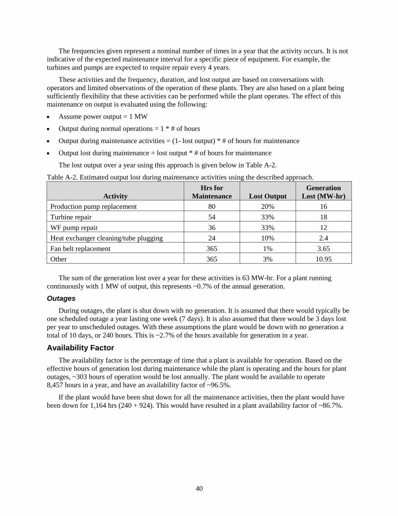
40

The frequencies given represent a nominal number of times in a year that the activity occurs. It is not indicative of the expected maintenance interval for a specific piece of equipment. For example, the turbines and pumps are expected to require repair every 4 years.

These activities and the frequency, duration, and lost output are based on conversations with operators and limited observations of the operation of these plants. They are also based on a plant being sufficiently flexibility that these activities can be performed while the plant operates. The effect of this maintenance on output is evaluated using the following:

• Assume power output = 1 MW

• Output during normal operations = 1 * # of hours

• Output during maintenance activities = (1- lost output) * # of hours for maintenance

• Output lost during maintenance = lost output * # of hours for maintenance

The lost output over a year using this approach is given below in Table A-2.

Table A-2. Estimated output lost during maintenance activities using the described approach.

Activity Hrs for

Maintenance Lost Output Generation

Lost (MW-hr) Production pump replacement 80 20% 16 Turbine repair 54 33% 18 WF pump repair 36 33% 12 Heat exchanger cleaning/tube plugging 24 10% 2.4 Fan belt replacement 365 1% 3.65 Other 365 3% 10.95

The sum of the generation lost over a year for these activities is 63 MW-hr. For a plant running

continuously with 1 MW of output, this represents ~0.7% of the annual generation.

Outages During outages, the plant is shut down with no generation. It is assumed that there would typically be

one scheduled outage a year lasting one week (7 days). It is also assumed that there would be 3 days lost per year to unscheduled outages. With these assumptions the plant would be down with no generation a total of 10 days, or 240 hours. This is ~2.7% of the hours available for generation in a year.

Availability Factor The availability factor is the percentage of time that a plant is available for operation. Based on the

effective hours of generation lost during maintenance while the plant is operating and the hours for plant outages, ~303 hours of operation would be lost annually. The plant would be available to operate 8,457 hours in a year, and have an availability factor of ~96.5%.

If the plant would have been shut down for all the maintenance activities, then the plant would have been down for 1,164 hrs (240 + 924). This would have resulted in a plant availability factor of ~86.7%.

41

Net Capacity Factor Over the life of the project, a plant’s NCF would be based on the plant availability and the impact of

the changes to both the ambient temperature and the resource productivity. In GETEM, the effects of changes in the resource productivity are considered separately (see Appendix A9). GETEM’s specified NCF includes the effect of plant availability and the ambient temperature on power generation. Because it excludes the effect of a declining resource’s productivity, the specified value is effectively what one would expect during the initial operation of the plant.

To estimate the effect of the ambient temperature and plant availability on generation, the annual output from a plant was estimated using the hourly temperature profile at Reno, Nevada over a year. The design output for the plant was based on the mean temperature for the annual profile used for Reno. On an hourly basis, the available energy (exergy) of the geothermal fluid was calculated using the fixed geothermal temperature and the varying ambient temperature. A correlation relating the impact of the ambient temperature on the second law efficiency was used to determine the plant performance for each hour (generally as the ambient temperature deviates from the design temperature, the second law efficiency decreases). Power output at a given hour during the year was the product of the available energy and the conversion efficiency (which are functions of the ambient temperature), an assumed geothermal flow rate, and the plant availability (96.5%). The analysis assumed that there was an operating limit placed on the generator output during the periods with a low ambient temperature (120% of nameplate); if the calculated output exceeded 20% of design, 120% of design was used for that hourly output.

The hourly plant output was totaled for the entire year, and that value was compared to the output that would have occurred if the plant had operated at its design output for 8,760 hours (24 hours per day*365 days). The ratio of the two values is the NCF.

Table A-3 below shows the results for a 15 MW plant operating with different resource temperatures. (Note that geothermal flow rate and conversion efficiency differ for each resource temperature).

Table A-3. Results for a 15 MW plant operating with different resource temperatures. Resource

Temperature Annual Calculated Output (MW · h)

Annual Output at Design (MW · h) Net Capacity Factor

100°C 123,776 131,400 94.2% 125°C 124,882 131,400 95% 150°C 125,380 131,400 95.4% 175°C 125,544 131,400 95.5% 100°C 125,556 131,400 95.6%

This evaluation is the basis for the default value of 95% that is used in GETEM for the net capacity

factor. Though a similar evaluation has not been made for flash plants, there is an expectation that the value would be similar. Flash plants would not experience the same sensitivity to the ambient temperature because they utilize evaporative heat rejection systems and typically utilize higher temperature resources. Because of the flashing, they could have more generation lost to issues associated with scaling. The assumption is that these two effects negate each other, and the same default is used for both plant types.

42

The net capacity factor of an operating plant will reflect the effect of a decline in resource productivity. GETEM accounts for this by estimating the effect of a decline in the geothermal fluid temperature on the power generation. This estimate is made for 12 intervals annually for the operating life of the project and incorporated into the LCOE calculation. For a binary plant that experiences a decline of 0.5% annually in the geothermal temperature (from an initial value of 175°C), the power output decreases by ~43% over 30 years. In the EERE methodology, the decrease in output over time is depicted as a declining net capacity factor used in calculating the present value of the power generated over the life of the project. In this scenario, the capacity factor would have effectively decreased from 95% to 54% at the end of 30 years.

43

A2: SCHEDULE Based on the input (default or revised) provided, GETEM develops a project schedule that is utilized

in determining the present value of a project’s pre-operational costs at the start of plant operation. This present value is used in the LCOE calculation that is reported.

The input used:

• Duration of the permitting activity for exploration and early drilling activities

• Duration of exploration phase

• Duration of drilling phase (including stimulation)

• Duration of installing the field gathering system

• Duration of period to establish plant design and finalize the PPA

• Duration of permitting for plant and well field (utilization permit)

• Duration to construct and startup power plant.

Using this input, a project schedule is developed using the following values that are built in to the approach used and cannot be revised.

• Exploration drilling begins 0.5 year after the start of the exploration phase.

• The duration of the drilling activity that occurs after the PPA is obtained is based on the remaining well field capacity that has to be developed to obtain the PPA and the duration of the plant construction; a minimum of 1 month of drilling activity occurs after the PPA is obtained.

𝐷𝐷𝑃𝑃𝑃𝑃𝑆𝑆𝑆𝑆𝑃𝑃𝑃𝑃𝑃𝑃 𝑆𝑆𝑓𝑓𝑃𝑃𝑃𝑃𝑃𝑃 𝑃𝑃𝑃𝑃𝑃𝑃 = (1 − 𝑃𝑃𝑃𝑃𝑆𝑆𝑆𝑆 𝑓𝑓𝑃𝑃𝑃𝑃𝑆𝑆𝑑𝑑 𝑃𝑃𝑆𝑆𝑃𝑃𝑆𝑆𝑃𝑃𝑃𝑃𝑃𝑃𝑐𝑐 𝑏𝑏𝑃𝑃𝑓𝑓𝑃𝑃𝑃𝑃𝑃𝑃 𝑃𝑃𝑃𝑃𝑃𝑃) ∗ 𝑃𝑃𝑆𝑆𝑆𝑆𝑃𝑃𝑃𝑃 𝑃𝑃𝑃𝑃𝑃𝑃𝑆𝑆𝑃𝑃𝑃𝑃𝑃𝑃𝑃𝑃𝑃𝑃𝑃𝑃𝑃𝑃𝑃𝑃

If no well field capacity has to be developed to get the PPA, the completion of the well field drilling will occur concurrently with the plant construction.

• The duration of the drilling activity that occurs before the PPA is the difference between the total time for the drilling phase and the duration of the drilling activity after the PPA is obtained.

• The durations of the well field stimulation and the installation of the field gathering system both before and after the PPA is obtained are determined in the same manner as determining the time for the drilling activities for these periods.

• It is assumed that the costs for engineering the plant design and construction are equally divided before and after the PPA is obtained. Those engineering costs after the PPA is obtained are incurred during the initial half of the period identified for the plant construction and startup.

• The geothermal pump installation is concurrent with the plant construction.

• The installation of transmission lines is concurrent with the plant construction.

• Plant construction and startup activity begins immediately after the PPA is obtained.

Though obtaining the PPA is the focal point in the project schedule, GETEM develops the schedule by working backward from the start of operations through the initial permitting activities for exploration.

44

With the assumption that plant construction and startup begins immediately after the PPA, this duration establishes when the PPA is obtained relative to the start of operation. The level of field capacity that must be developed prior to obtaining the PPA establishes when the drilling phase begins, which also represents the end of the exploration activities. Immediately prior to the start of the exploration work, the permitting is done for exploration. Some activities are assumed to occur concurrently (e.g., the drilling and installation of the field gathering system needed to obtain the PPA, as well as permitting and completing the well field and installing and operating the power plant).

Figure A-1 below shows this schedule using the model defaults for activity duration for a scenario with a hydrothermal resource and a binary power plant.

Figure A-1. Snapshot of GETEM’s project activity schedule using default for hydrothermal resource using a binary power plant.

If the duration of the drilling activity is increased from 2.5 to 3 years with 100% of the well field capacity being developed, the updated schedule in Figure A-2 below reflects the revised input.

Figure A-2. Snapshot of GETEM’s project activity schedule with revised input.

Note that the inputs used to determine this schedule are not all in the economics input section on the Scenario Definition worksheet. The inputs for the time needed for permitting is in the Permitting input section of this sheet. The definition of the amount of well field capacity to get a PPA is in the Drilling Activities section.

45

The schedule of pre-operation activities is used to determine the present value of the costs for these project activities at the start of plant operation. This point in time is time zero (0) in GETEM for determining the present value of all project costs and revenues that are used in determining the LCOE, as well as the contributions of different activities to this generation cost. For example, using GETEM’s defaults, the overnight exploration costs for the scenario shown above is $607/kW of sales. Using the default schedule and discount rates, the present value of exploration at the beginning of plant operations would be $797/kW. With the increase in the project duration for the revised scenario indicated, the present value increases to $882/kW. This increased the model’s LCOE estimate by ~3%.

GETEM also allows one to depict the potential impact of risk on a project, using higher discount rates for those activities with the greatest perceived risk. If the discount rate for the exploration activities was increased from 7% to 20% and all other inputs were kept at the default value, the present value in the previous example would increase from $797/kW to $1,271/kW, resulting in ~6% increase in the estimated LCOE. If the revised schedule discussed above were used with the higher discount rate, the present value would increase to $1,666/kW and result in a ~13% increase in the LCOE.

GETEM does allow for these early project costs to be discounted at a lower rate (the same as that used by the power plant) once the PPA is obtained. With this option, the present value of the exploration costs would be $1,324/kW, which produces a LCOE that is ~9% more than the default estimate.

When GETEM uses the project schedule and discount rates to determine the present value of cost, it assumes that the costs are spread evenly over the activity duration. In addition, the present value of the costs is calculated assuming that they are incurred at the end of a year. For instance, costs that are incurred 6 to 7 years prior to startup are discounted over a 6 year period; those incurred in the year prior to the start of operation are not discounted.

46

A3: GETEM LCOE CALCULATION GETEM’s calculation of the LCOE for the defined project replicates a discounted cash flow method

that is provided by the EERE to GTO as a recommended approach for determining the generation cost for renewables. In this calculation,

𝐿𝐿𝐿𝐿𝑂𝑂𝐿𝐿 = 𝐿𝐿𝐿𝐿𝐿𝐿𝑃𝑃𝑃𝑃(𝑄𝑄)

,

where

LCC is total lifecycle cost

PV(Q) is present value of annual energy production (Q).

𝐿𝐿𝐿𝐿𝐿𝐿 = 𝑃𝑃𝑃𝑃(𝐼𝐼𝐿𝐿𝐿𝐿)∙�1−𝜏𝜏∙𝑃𝑃𝑃𝑃(𝐷𝐷)�+(1−𝜏𝜏)∙𝑃𝑃𝑃𝑃(𝑂𝑂&𝑀𝑀)(1−𝜏𝜏)

where

PV(ICC) is present value of installed capital cost (ICC)

PV(D) is present value of depreciation (D)

PV(O&M) is present value of operation and maintenance cost (O&M)

𝜏𝜏 is the effective tax rate (%).

The present values of both costs and power are determined at the start of power generation and sales. This point represents time = “0.” Note that this relationship for LCC does not include the royalty payments that are included in GETEM’s LCOE estimate.

Capital Costs The installed capital costs that are included in the LCOE determination are both those occurring prior

to the start of operations and those incurred once operation begins. In GETEM, the only capital costs that are incurred after operation are those associated with replacement of the well field that may occur if the decline in resource productivity reaches a maximum threshold.

Those costs that are included in the determination of the pre-operational capital costs include:

- Leasing and permitting for exploration and early drilling activities - Exploration activities (not associated with drilling) - Exploration drilling (both small diameter and full-sized wells and any well stimulation) - Drilling phase prior to obtaining PPA (both drilling and well stimulation) - Drilling phase after obtaining PPA (both drilling and well stimulation) - Permitting power plant and completion of well field - Engineering prior to PPA - Field gathering system activities prior to PPA - Field gathering system activities prior to PPA - Geothermal pump installation - Plant construction and startup GETEM assumes that the costs for these activities are spread evenly over the duration identified for

each. In calculating the present value of the activity cost, GETEM considers when the costs occur within the project schedule. For example, if the permitting for the plant and well field occurred over a 1-year period from year −3.5 to year −2.5, GETEM would assign half the cost to year −3 and half to year −2.

47

For each pre-operation activity having assigned costs and schedule, the present value at startup is determined using the following relationship:

PV(OCC𝑝𝑝𝑎𝑎𝑛𝑛𝑓𝑓𝑎𝑎𝑓𝑓𝑛𝑛𝑎𝑎) = ��𝑂𝑂𝐿𝐿𝐿𝐿𝑝𝑝𝑎𝑎𝑛𝑛𝑓𝑓𝑎𝑎𝑓𝑓𝑛𝑛𝑎𝑎�𝑛𝑛

(1 + 𝑑𝑑)𝑛𝑛

𝑛𝑛

𝑛𝑛=0

where

OCCactivity is the overnight capital cost for the activity,

t is the time when the activity begins in the project schedule, and

d is the discount rate.

GETEM allows for evaluation in which all costs incurred before the PPA are subsequently discounted at a lower rate once the PPA is obtained. With this option, the determination of the present value for the activities is adjusted as shown below.

PV(OCC𝑝𝑝𝑎𝑎𝑛𝑛𝑓𝑓𝑎𝑎𝑓𝑓𝑛𝑛𝑎𝑎)𝑃𝑃𝑃𝑃𝑃𝑃 = ��𝑂𝑂𝐿𝐿𝐿𝐿𝑝𝑝𝑎𝑎𝑛𝑛𝑓𝑓𝑎𝑎𝑓𝑓𝑛𝑛𝑎𝑎�𝑛𝑛

(1 + 𝑑𝑑𝑓𝑓)𝑛𝑛

𝑛𝑛−𝑛𝑛𝑃𝑃𝑃𝑃𝑃𝑃

𝑛𝑛=0

where

PV(OCCactivity)PPA is the present value of the activity cost at the point in the project schedule when the PPA is obtained,

tPPA is the time in the project schedule when the PPA is obtained, and

di is the initial discount rate.

This defines the present value of the project activity at the point in time when the PPA is obtained, at which time these costs are assumed to be re-financed. From this point forward to startup, a lower discount rate is applied (same as power plant) to the PV at this point to determine the activity’s present value at startup.

PV(OCC𝑝𝑝𝑎𝑎𝑛𝑛𝑓𝑓𝑎𝑎𝑓𝑓𝑛𝑛𝑎𝑎) = �PV(OCC𝑝𝑝𝑎𝑎𝑛𝑛𝑓𝑓𝑎𝑎𝑓𝑓𝑛𝑛𝑎𝑎)𝑃𝑃𝑃𝑃𝑃𝑃 + �𝑂𝑂𝐿𝐿𝐿𝐿𝑝𝑝𝑎𝑎𝑛𝑛𝑓𝑓𝑎𝑎𝑓𝑓𝑛𝑛𝑎𝑎�𝑛𝑛

(1 + 𝑑𝑑2)𝑛𝑛

𝑛𝑛𝑃𝑃𝑃𝑃𝑃𝑃

𝑛𝑛=0

In this relationship d2 is the discount rate applied once the PPA is obtained.

The present value of the project at startup (time = 0) is the sum of the present values determined for each of the activities.

𝑃𝑃𝑃𝑃(𝑂𝑂𝐿𝐿𝐿𝐿) = �𝑃𝑃𝑃𝑃(𝑂𝑂𝐿𝐿𝐿𝐿)𝑝𝑝𝑎𝑎𝑛𝑛𝑓𝑓𝑎𝑎𝑓𝑓𝑛𝑛𝑎𝑎

GETEM also uses the PVs for the individual activities to determine the relative contributions of different project phases/activities to the total LCOE determined for the project. This allows GTO to identify which project elements are the major drivers for the LCOE.

The present value of the installed capital cost is the sum of the present values of both overnight capital costs and the replacement capital costs (RCC) incurred over the project life.

PV(ICC) = 𝑃𝑃𝑃𝑃(𝑂𝑂𝐿𝐿𝐿𝐿) + �(𝑅𝑅𝐿𝐿𝐿𝐿)𝑛𝑛

(1 + 𝑑𝑑)𝑛𝑛

𝑝𝑝𝑝𝑝𝑔𝑔𝑝𝑝𝑛𝑛𝑎𝑎𝑛𝑛 𝑓𝑓𝑓𝑓𝑓𝑓𝑛𝑛

𝑛𝑛=1

In this relationship the discount rate (d) is the specified discount rate for the project once operation begins. It determines present value of the replacement costs, deprecation, O&M costs, and power generation at the start of operation. In GETEM, the only replacement costs considered are those associated with the replacement of the well field. GETEM does not include inflation in its estimates, so

48

the costs used for well field replacement are the overnight costs for the full-size well drilling and field gathering system activities, exclusive of any “failed” wells that are drilled prior to the startup of the facility.

The periodic replacement of the geothermal production pumps during operation of the facility are not considered a replacement capital cost, though they are included in the pre-operational capital costs for the field gathering system. In GETEM, this pump replacement is included as an O&M cost for the facility.

Depreciation GETEM utilizes a 5-year MACRS depreciation schedule (Internal Revenue Service 2015). The values

used are given below in Table A-4.

Table A-4. Five-year MACRS depreciation schedule. Year Rate

1 20% 2 32% 3 19.25 4 11.52% 5 11.52% 6 5.76%

GETEM applies this schedule to the present value of the overnight capital costs once operation begins

(year 1 as indicated in the table). In the determination of the LCC, the present value of depreciation (PV[D]) is applied to the PV(ICC); the PV(D) used is the present value of the rates in the above schedule for the period shown in the table:

𝑃𝑃𝑃𝑃(𝐷𝐷) = �(𝑑𝑑𝑃𝑃𝑃𝑃𝑃𝑃𝑃𝑃𝑃𝑃𝑃𝑃𝑆𝑆𝑃𝑃𝑃𝑃𝑃𝑃𝑃𝑃 𝑃𝑃𝑆𝑆𝑃𝑃𝑃𝑃)𝑛𝑛

(1 + 𝑑𝑑)𝑛𝑛

6

𝑛𝑛=1

49

Operating and Maintenance (O&M) In the determination of the LCOE, GETEM assumes that O&M are an annual fixed cost that include:

• Labor

• Plant maintenance

• Well maintenance

• Gathering system maintenance

• Makeup water

• Pump replacement/repair

• Taxes and insurance.

Royalties could also be considered an O&M expense, but GETEM determines that contribution separately when determining the LCOE:

PV(O&M) = �(𝑆𝑆𝑃𝑃𝑃𝑃𝑃𝑃𝑆𝑆𝑆𝑆 𝑂𝑂&𝑀𝑀 𝑃𝑃𝑃𝑃𝑆𝑆𝑃𝑃)𝑛𝑛

(1 + 𝑑𝑑)𝑛𝑛

𝑝𝑝𝑝𝑝𝑔𝑔𝑝𝑝𝑛𝑛𝑎𝑎𝑛𝑛 𝑓𝑓𝑓𝑓𝑓𝑓𝑛𝑛

𝑛𝑛=1

Power Generation GETEM’s LCOE calculation is based on the present value of the power sales over the life of the

project, or the sum of the sales discounted at a specified discount rate over the project life.

PV(Q) = �(𝑃𝑃𝑃𝑃𝑃𝑃𝑃𝑃𝑃𝑃 𝑆𝑆𝑆𝑆𝑆𝑆𝑃𝑃𝑆𝑆)𝑛𝑛

(1 + 𝑑𝑑)𝑛𝑛

𝑝𝑝𝑝𝑝𝑔𝑔𝑝𝑝𝑛𝑛𝑎𝑎𝑛𝑛 𝑓𝑓𝑓𝑓𝑓𝑓𝑛𝑛

𝑛𝑛=1

If power sales were constant over the entire life of the project, the determination of their present value would be straightforward. This could occur if the geothermal resource operated with no change in resource productivity over the life of the project. This is unlikely to occur as nearly all geothermal resources experience some productivity decline that is manifested as a decreasing fluid temperature or flow rate. A review of production data from binary plants indicates that the geothermal temperatures have decreased since the beginning of operation. Most of these plants also experience some change in flow rate over their life, with flow generally increasing as operators attempt to maintain power sales. The relative magnitude of these increases in flow varies from facility to facility, as well as with time at a given facility.

GETEM estimates the impact of declining productivity on sales based on a temperature decline with time, with the flow assumed constant. The approach used is not amenable to considering both flow and temperature, and because decreasing temperature is more likely to occur, it is used to characterize the effect of declining resource productivity on power sales.

The impact of a declining resource temperature on power sales is estimated over the life of the project. Plant output is determined for 12 equal increments for each year of the project life; this calculation is based on the geothermal temperature at a point in time, an assumed ambient temperature (10°C or 50°F for binary plants), and the initial performance of the plant. The two temperatures (source and sink) determine the available energy (specific exergy), which is the ideal work that could be done by a conversion system using reversible processes. No actual conversion system can achieve this ideal performance. The fraction of this ideal work that is converted to useful work (power) is the second law efficiency of the conversion system or power plant.

50

The second law efficiency is also impacted by the resource temperature decline. This efficiency will be at its maximum when operating near the design geothermal and ambient conditions. As the resource temperature declines, so will this conversion efficiency. GETEM’s estimates of net output from the power plant include this effect on efficiency.

Power sales is the difference between the plant output and the geothermal pumping power. In GETEM it is assumed that the geothermal pumping power does not change from what is determined at startup (i.e., the geothermal flow remains constant, the hydraulic performance of the reservoir does not change, and the effect of temperature decline on density heads in both the production and injection well negate each other). The effect of temperature decline on power is illustrated in Figure A-3 below. Note that this is an example based on a postulated initial plant performance and geothermal pumping power.

Figure A-3. The effect of temperature decline on power.

The decline in the available energy shown in this figure is indicative of the level of decline that will be experienced under ideal conditions with no geothermal pumping. Because it is improbable that one could increase the conversion efficiency as the temperature declines, sustaining power generation would require an increased flow rate. (Note that increasing flow would likely further lower the second law conversion efficiency.)

Again, GETEM’s methodology does not allow for increasing flow rate. To represent an operator’s use of new wells to supplement production or replace wells to mitigate the effect on sales, GETEM assumes that there is a maximum allowable temperature decline, after which the entire well field is replaced, and the production temperature and plant output return to their initial design values.

For the 175°C resource temperature in the above figure, GETEM’s default for the maximum allowable temperature decline is slightly less than 25°C. The maximum decline is based on a curve fit of the end of project life temperature taken from the EPRI’s report (EPRI 1996). This decline corresponds to a ~10% decrease in the Carnot efficiency for all resource temperatures. Using the GETEM default, the well field depicted in this figure would be replaced once the temperature had declined to ~150°C; at this point power sales would have decreased by ~44%.

51

GETEM uses an annual decline rate to characterize the temperature decline of the geothermal resource. Figure A-4 depicts the decline rate that would trigger a well field replacement. These decline rates preclude the replacement of the well field during the last 5 years of the project life—this exclusion is built into GETEM and effectively allows for a higher decline rate before triggering the replacement of the well field.

Figure A-4. Rate of annual temperature decline that would trigger well field replacement.

For GETEM’s default of a 30-year project life, if a 200°C resource temperature declined at a rate higher than 0.65%, the well field would be replaced before the plant reached 25 years of operation. This decline rate produces a 1.3°C (2.3°F) temperature decline the first year, with slightly less in the subsequent years. With no replacement, by the end of the project (30 years), the 200°C resource would have declined in temperature to ~165°C with the 0.65% annual decline rate.

Though GETEM calculates the effect of temperature decline on power output on a monthly basis, the present value calculation of the power generated uses the power output at the end of a year to determine the annual generation for that year. For a representative temperature decline rate, the annual generation based on the plant’s year-end power output is 0.5 to 1.2% lower than when determined on a monthly basis, with the difference increasing each year throughout the life of the project. The total generation over a typical 30-year project will be ~1% higher if generation is established on a monthly rather than a year-end basis; the impact on LCOE would be similar. Though conservative, the use of year-end power to determine annual generation is consistent with the EERE methodology provided.

The EERE methodology for determining LCOE depicts the impact of a declining resource temperature as a decline in the capacity factor with time. A capacity factor is the ratio of the actual generation over a year to what would have been produced if the unit operated continuously throughout the year at a “design” value. NCF is a GETEM input. The basis of the power in this value is the net output from the plant (sales plus geothermal pumping power). The value includes the effects of maintenance, outages, and the ambient temperature on annual generation. For the depiction of the effect of temperature decline on power sales, it is assumed that the capacity factor based on power sales and that based on net plant output will behave similarly. With this assumption, GETEM’s NCF input is used in the EERE methodology as the initial (design) capacity factor based on power sales.

52

The degradation in the capacity factor is determined using the following relationship: 𝛿𝛿𝐿𝐿𝐶𝐶 = 1 − 𝑃𝑃𝑎𝑎 , where

𝑃𝑃 =ln �

𝑆𝑆𝑆𝑆𝑆𝑆𝑃𝑃𝑆𝑆@ 𝑛𝑛𝑟𝑟𝑆𝑆𝑆𝑆𝑆𝑆𝑃𝑃𝑆𝑆𝑓𝑓𝑛𝑛𝑑𝑑𝑓𝑓𝑔𝑔𝑛𝑛

�

𝑃𝑃𝑝𝑝

and δCF is the annual decline rate for the capacity factor (CF)

salest is the power sales at time t

salesdesign is the design power sales.

tr is either the project life, or the time at which the 1st well field replacement occurs.

The power sales at any point in time (n) is 𝑃𝑃𝑃𝑃𝑃𝑃𝑃𝑃𝑃𝑃 𝑆𝑆𝑆𝑆𝑆𝑆𝑃𝑃𝑆𝑆𝑛𝑛 = 𝑃𝑃𝑃𝑃𝑃𝑃𝑃𝑃𝑃𝑃 𝑆𝑆𝑆𝑆𝑆𝑆𝑃𝑃𝑆𝑆𝑓𝑓𝑛𝑛𝑑𝑑𝑓𝑓𝑔𝑔𝑛𝑛 ∗ 𝐿𝐿𝐶𝐶𝑓𝑓𝑛𝑛𝑑𝑑𝑓𝑓𝑔𝑔𝑛𝑛 ∗ (1 − 𝛿𝛿𝐿𝐿𝐶𝐶)𝑛𝑛

The present value of the power sales for the project is (with no well field replacement)

PV(Q) = 𝑃𝑃𝑃𝑃𝑃𝑃𝑃𝑃𝑃𝑃 𝑆𝑆𝑆𝑆𝑆𝑆𝑃𝑃𝑆𝑆𝑓𝑓𝑛𝑛𝑑𝑑𝑓𝑓𝑔𝑔𝑛𝑛 ∗ 𝐿𝐿𝐶𝐶𝑓𝑓𝑛𝑛𝑑𝑑𝑓𝑓𝑔𝑔𝑛𝑛 �(1 − 𝛿𝛿𝐿𝐿𝐶𝐶)𝑛𝑛

(1 + 𝑑𝑑)𝑛𝑛

𝑝𝑝𝑝𝑝𝑔𝑔𝑝𝑝𝑛𝑛𝑎𝑎𝑛𝑛 𝑓𝑓𝑓𝑓𝑓𝑓𝑛𝑛

𝑛𝑛=1

With well field replacement, the present value of the sales is

𝑃𝑃𝑃𝑃(𝑄𝑄) = 𝑃𝑃𝑃𝑃𝑃𝑃𝑃𝑃𝑃𝑃 𝑆𝑆𝑆𝑆𝑆𝑆𝑃𝑃𝑆𝑆𝑓𝑓𝑛𝑛𝑑𝑑𝑓𝑓𝑔𝑔𝑛𝑛 ∗ 𝐿𝐿𝐶𝐶𝑓𝑓𝑛𝑛𝑑𝑑𝑓𝑓𝑔𝑔𝑛𝑛∑ �1 − 𝛿𝛿𝑎𝑎𝑓𝑓�

𝑛𝑛 + ∑ �1 − 𝛿𝛿𝑎𝑎𝑓𝑓�𝑛𝑛−𝑛𝑛𝑟𝑟2∗𝑛𝑛𝑟𝑟

𝑛𝑛=1+𝑛𝑛𝑟𝑟 + ∑ (1 − 𝛿𝛿𝐶𝐶𝐷𝐷)𝑛𝑛−2∗𝑛𝑛𝑟𝑟3∗𝑛𝑛𝑟𝑟𝑛𝑛=1+2∗𝑛𝑛𝑟𝑟

𝑛𝑛𝑟𝑟𝑛𝑛=1 + ⋯

∑ (1 + 𝑑𝑑𝑝𝑝)𝑛𝑛𝑝𝑝𝑝𝑝𝑔𝑔𝑝𝑝𝑛𝑛𝑎𝑎𝑛𝑛 𝑓𝑓𝑓𝑓𝑓𝑓𝑛𝑛𝑛𝑛=1

In this relationship, tr is the time when well field replacement first occurs, and dr is the discount rate used for costs and revenues once operation begins. In GETEM, the well field will continue to be replaced, provided sufficient resource potential was found during exploration to allow for re-drilling the well field one or more times, and the replacement does not occur in the last 5 years of the project life.

With a high rate of temperature decline and insufficient resource potential for well field makeup, at some point the power output will go to zero. At this point an Error/Warnings message will be received that power output is zero before the end of project life. Depending upon the scenario being evaluated, the model may or may not continue to estimate the present value of subsequent power generation (which will be negative). If it does, it will continue to do so through the end of the inputted project life. Similarly, it will continue to include in the present value of O&M costs through the end of the project. This leads to an overestimate of both the costs and power generation (and an underestimate of royalties) used to determine the LCOE. As a consequence, once this error occurs, the estimates produced by GETEM are not valid.

These issues do not occur when using the DCF on the DCF-COE worksheet. However, when using the DCF, the model cannot solve for the level of plant performance that minimizes the LCOE. If one uses the DCF to determine the LCOE, one should first optimize binary performance to minimize the LCOE determined using the EERE methodology based on declining capacity factor and then determine the LCOE with the DCF. This will define a plant performance metric (brine effectiveness) that can be manually adjusted until the LCOE is a minimum.

The issues associated with the power going to zero before the end of the project life are also relevant to the FCR method. This methodology correctly accounts for the sales and revenues going to zero, but a 30-year project life is inherent to the fixed charge rate method in GETEM.

Royalties The default for the annual royalty payments on LCOE is based on the BLM schedule for royalties, in

which 1.75% of the annual revenues are paid through the first 10 years of operation, and 3.5% of annual revenues are paid after 10 years.

53

In determining the contribution of royalty payments to the LCOE, GETEM first determines the present value of the power generation in the initial period. The method used is the same as discussed in the previous section for determining the present value of power generation for the project life. Once that value is determined, it is used with the present value of all power generation to determine the levelized value of the royalties, which is representative of the present value of the royalties relative to the present value of the total revenues.

𝑆𝑆𝑃𝑃𝑙𝑙𝑃𝑃𝑆𝑆𝑃𝑃𝑙𝑙𝑃𝑃𝑑𝑑 𝑃𝑃𝑃𝑃𝑐𝑐𝑆𝑆𝑆𝑆𝑃𝑃𝑃𝑃𝑃𝑃𝑆𝑆 =�𝑅𝑅𝑅𝑅𝑓𝑓𝑛𝑛𝑓𝑓𝑛𝑛𝑓𝑓𝑝𝑝𝑓𝑓 × 𝑃𝑃𝑃𝑃 𝑃𝑃𝑃𝑃𝑃𝑃𝑃𝑃𝑃𝑃𝑓𝑓𝑛𝑛𝑓𝑓𝑛𝑛𝑓𝑓𝑝𝑝𝑓𝑓 + 𝑅𝑅𝑅𝑅𝑓𝑓𝑓𝑓𝑛𝑛𝑝𝑝𝑓𝑓 × �𝑃𝑃𝑃𝑃 𝑃𝑃𝑃𝑃𝑃𝑃𝑃𝑃𝑃𝑃𝑓𝑓𝑓𝑓𝑓𝑓𝑛𝑛 − 𝑃𝑃𝑃𝑃 𝑃𝑃𝑃𝑃𝑃𝑃𝑃𝑃𝑃𝑃𝑓𝑓𝑛𝑛𝑓𝑓𝑛𝑛𝑓𝑓𝑝𝑝𝑓𝑓��

𝑃𝑃𝑃𝑃 𝑃𝑃𝑃𝑃𝑃𝑃𝑃𝑃𝑃𝑃𝑓𝑓𝑓𝑓𝑓𝑓𝑛𝑛

where

RRinitial is the royalty rate (1.75%) for the initial period (10 years)

PV Powerinitial is the present value of the power generated during the initial period RRfinal is the royalty rate (3.5%) after the initial period

PV Powerlife is the present value of the power generated during the initial period (PV[Q], the value discussed in the previous section)

Royalties are based on the final LCOE and the annual power production. The next section describes how this final determination of LCOE is accomplished.

LCOE Determination In the calculation of the LCOE, GETEM uses the levelized royalties, levelized capital costs and

levelized O&M costs as depicted here:

𝐿𝐿𝐿𝐿𝑂𝑂𝐿𝐿 =(𝑆𝑆𝑃𝑃𝑙𝑙𝑃𝑃𝑆𝑆𝑃𝑃𝑙𝑙𝑃𝑃𝑑𝑑 𝑃𝑃𝑆𝑆𝑃𝑃𝑃𝑃𝑃𝑃𝑆𝑆𝑆𝑆 𝑃𝑃𝑃𝑃𝑆𝑆𝑃𝑃 + 𝑆𝑆𝑃𝑃𝑙𝑙𝑃𝑃𝑆𝑆𝑃𝑃𝑙𝑙𝑃𝑃𝑑𝑑 𝑂𝑂&𝑀𝑀 𝑃𝑃𝑃𝑃𝑆𝑆𝑃𝑃)

(1 − 𝑆𝑆𝑃𝑃𝑙𝑙𝑃𝑃𝑆𝑆𝑃𝑃𝑙𝑙𝑃𝑃𝑑𝑑 𝑃𝑃𝑃𝑃𝑐𝑐𝑆𝑆𝑆𝑆𝑃𝑃𝑃𝑃𝑃𝑃𝑆𝑆)

The determination of the levelized royalties is discussed in the previous section. The levelized capital costs include the initial project capital costs and any subsequent replacement capital costs (PV[ICC] in the previous discussion).

𝑆𝑆𝑃𝑃𝑙𝑙𝑃𝑃𝑆𝑆𝑃𝑃𝑙𝑙𝑃𝑃𝑑𝑑 𝑃𝑃𝑆𝑆𝑃𝑃𝑃𝑃𝑃𝑃𝑆𝑆𝑆𝑆 𝑃𝑃𝑃𝑃𝑆𝑆𝑃𝑃𝑆𝑆 =𝑃𝑃𝑃𝑃(𝐼𝐼𝐿𝐿𝐿𝐿) × (1 − 𝜏𝜏 × 𝑃𝑃𝑃𝑃(𝑑𝑑𝑃𝑃𝑃𝑃𝑃𝑃𝑃𝑃𝑃𝑃𝑃𝑃𝑆𝑆𝑃𝑃𝑃𝑃𝑃𝑃𝑃𝑃))

(1 − 𝜏𝜏)𝑃𝑃𝑃𝑃(𝑄𝑄)

The levelized O&M cost is determined using the following relationship:

𝑆𝑆𝑃𝑃𝑙𝑙𝑃𝑃𝑆𝑆𝑃𝑃𝑙𝑙𝑃𝑃𝑑𝑑 𝑂𝑂&𝑀𝑀 𝑃𝑃𝑃𝑃𝑆𝑆𝑃𝑃𝑆𝑆 =𝑃𝑃𝑃𝑃(𝑂𝑂&𝑀𝑀) × ((1 + 𝑑𝑑)𝑝𝑝𝑝𝑝𝑔𝑔𝑝𝑝𝑛𝑛𝑎𝑎𝑛𝑛 𝑓𝑓𝑓𝑓𝑓𝑓𝑛𝑛 − 1)

(𝑑𝑑 × (1 + 𝑑𝑑)𝑝𝑝𝑝𝑝𝑔𝑔𝑝𝑝𝑛𝑛𝑎𝑎𝑛𝑛 𝑓𝑓𝑓𝑓𝑓𝑓𝑛𝑛)𝑃𝑃𝑃𝑃(𝑄𝑄)

GETEM determines LCOE contributions from the following:

Capital costs:

- Exploration - Drilling - Field gathering system - Stimulation - Power plant - Permitting - Makeup drilling.

Operating costs:

54

- O&M labor - Maintenance for plant - Maintenance for well field and reservoir - Maintenance for gathering system - Water makeup - Production pump maintenance - Taxes and insurance - Royalties. The contribution from each of the capital cost contributors is:

𝐿𝐿𝐿𝐿𝑂𝑂𝐿𝐿𝑎𝑎𝑝𝑝𝑝𝑝𝑓𝑓𝑛𝑛𝑝𝑝𝑓𝑓 𝑎𝑎𝑔𝑔𝑑𝑑𝑛𝑛 =𝑃𝑃𝑃𝑃(𝑃𝑃𝑆𝑆𝑃𝑃𝑃𝑃𝑃𝑃𝑆𝑆𝑆𝑆 𝑃𝑃𝑃𝑃𝑆𝑆𝑃𝑃 𝑃𝑃𝑃𝑃𝑃𝑃𝑃𝑃𝑃𝑃𝑃𝑃𝑏𝑏𝑃𝑃𝑃𝑃𝑃𝑃𝑃𝑃𝑃𝑃) × (1 − 𝜏𝜏 × 𝑃𝑃𝑃𝑃(𝑑𝑑𝑃𝑃𝑃𝑃𝑃𝑃𝑃𝑃𝑃𝑃𝑃𝑃𝑆𝑆𝑃𝑃𝑃𝑃𝑃𝑃𝑃𝑃))

(1 − 𝜏𝜏)𝑃𝑃𝑃𝑃(𝑄𝑄)

The contribution of each of the operating costs (excluding royalties) is:

𝐿𝐿𝐿𝐿𝑂𝑂𝐿𝐿𝑂𝑂&𝑀𝑀 =𝑃𝑃𝑃𝑃(𝑆𝑆𝑃𝑃𝑃𝑃𝑃𝑃𝑆𝑆𝑆𝑆 𝑂𝑂&𝑀𝑀 𝑃𝑃𝑃𝑃𝑃𝑃𝑃𝑃𝑃𝑃𝑃𝑃𝑏𝑏𝑃𝑃𝑃𝑃𝑃𝑃𝑃𝑃𝑃𝑃) × ((1 + 𝑑𝑑)𝑝𝑝𝑝𝑝𝑔𝑔𝑝𝑝𝑛𝑛𝑎𝑎𝑛𝑛 𝑓𝑓𝑓𝑓𝑓𝑓𝑛𝑛 − 1)

(𝑑𝑑 × (1 + 𝑑𝑑)𝑝𝑝𝑝𝑝𝑔𝑔𝑝𝑝𝑛𝑛𝑎𝑎𝑛𝑛 𝑓𝑓𝑓𝑓𝑓𝑓𝑛𝑛)𝑃𝑃𝑃𝑃(𝑄𝑄)

The royalty contribution is:

𝐿𝐿𝐿𝐿𝑂𝑂𝐿𝐿𝑝𝑝𝑔𝑔𝑎𝑎𝑝𝑝𝑓𝑓𝑛𝑛𝑎𝑎 = 𝐿𝐿𝐿𝐿𝑂𝑂𝐿𝐿𝑛𝑛𝑔𝑔𝑛𝑛𝑝𝑝𝑓𝑓 × �𝑅𝑅𝑅𝑅𝑓𝑓𝑛𝑛𝑓𝑓𝑛𝑛𝑓𝑓𝑝𝑝𝑓𝑓 × 𝑃𝑃𝑃𝑃 𝑃𝑃𝑃𝑃𝑃𝑃𝑃𝑃𝑃𝑃𝑓𝑓𝑛𝑛𝑓𝑓𝑛𝑛𝑓𝑓𝑝𝑝𝑓𝑓 + 𝑅𝑅𝑅𝑅𝑓𝑓𝑓𝑓𝑛𝑛𝑝𝑝𝑓𝑓 × �𝑃𝑃𝑃𝑃 𝑃𝑃𝑃𝑃𝑃𝑃𝑃𝑃𝑃𝑃𝑓𝑓𝑓𝑓𝑓𝑓𝑛𝑛 − 𝑃𝑃𝑃𝑃 𝑃𝑃𝑃𝑃𝑃𝑃𝑃𝑃𝑃𝑃𝑓𝑓𝑛𝑛𝑓𝑓𝑛𝑛𝑓𝑓𝑝𝑝𝑓𝑓��

𝑃𝑃𝑃𝑃 𝑃𝑃𝑃𝑃𝑃𝑃𝑃𝑃𝑃𝑃𝑓𝑓𝑓𝑓𝑓𝑓𝑛𝑛

Other LCOE Methods The reported LCOE is determined using the EERE methodology described. There are two alternative

calculations of LCOE within GETEM that have been alluded to. One is a simple discounted cash flow method and the second is based on a fixed charge rate.

Discounted Cash Flow This calculation is on the DCF-COE worksheet. The capital costs and operating costs used in this

calculation are the same as those utilized in the EERE methodology. The calculation differs from that used in the EERE methodology in how power sales are determined. This approach uses the calculated year-end power output, while the EERE methodology bases power sales on the effect of a declining capacity factor. This worksheet has two macros: one each for the default and revised scenarios. Each macro varies the cost of electricity until the present values of all costs are equivalent to the present value of all revenues (a “0” cash flow). If there is no resource temperature decline, the cost of electricity determined should be equivalent to that determined using the EERE method.

If this method is used with binary plants, it is recommended that the default values be used for the revised scenario to establish a representative level for the plant performance. Revisions can be made to the inputs, and the macros run on this sheet to determine a cost of electricity. The optimal plant performance/minimum LCOE can iteratively be found by adjusting the brine effectiveness for the binary plant (Scenario Definition—Power Plant) and running the macros on the DCF-COE worksheet until the LCOE for the revised scenario is minimized.

Fixed Charge Rate The calculation of the LCOE using the FCR was used in the original versions of GETEM. Though

this calculation is also not reported, it has been retained in the model and can be used. The FCR is the fraction of the project capital costs that represents the annual cost for capitalized equipment and services. It includes the rate of return on equity and interest on debt, income taxes, property taxes, and insurance.

55

The default value of 10.8% was the rate last used when the FCR methodology was the basis for GETEM’s LCOE estimate in 2012. This was the value used in the EIA NEMS runs for the Annual Energy Outlook report (EIA 2015). A fixed project operating life of 30 years is inherent to GETEM’s FCR methodology for LCOE.

The LCOE for either the default or revised scenario is determined using the methodology described below.

𝑆𝑆𝑃𝑃𝑃𝑃𝑃𝑃𝑙𝑙𝑃𝑃𝑃𝑃𝑐𝑐 𝑃𝑃𝑙𝑙𝑃𝑃𝑃𝑃𝑃𝑃𝑃𝑃𝑃𝑃ℎ𝑃𝑃 𝑃𝑃𝑆𝑆𝑃𝑃𝑃𝑃𝑃𝑃𝑆𝑆𝑆𝑆 𝑃𝑃𝑃𝑃𝑆𝑆𝑃𝑃𝑝𝑝𝑛𝑛𝑝𝑝 𝑘𝑘𝑘𝑘 =𝑃𝑃𝑙𝑙𝑃𝑃𝑃𝑃𝑃𝑃𝑃𝑃𝑃𝑃ℎ𝑃𝑃 𝑃𝑃𝑆𝑆𝑃𝑃𝑃𝑃𝑃𝑃𝑆𝑆𝑆𝑆 𝑃𝑃𝑃𝑃𝑆𝑆𝑃𝑃𝑝𝑝𝑎𝑎𝑛𝑛𝑓𝑓𝑎𝑎𝑓𝑓𝑛𝑛𝑎𝑎

𝑑𝑑𝑃𝑃𝑆𝑆𝑃𝑃𝑃𝑃𝑃𝑃 𝑆𝑆𝑆𝑆𝑆𝑆𝑃𝑃𝑆𝑆𝑘𝑘𝑘𝑘

𝑆𝑆𝑃𝑃𝑃𝑃𝑃𝑃𝑙𝑙𝑃𝑃𝑃𝑃𝑐𝑐 𝑆𝑆𝑃𝑃𝑃𝑃𝑃𝑃𝑆𝑆𝑆𝑆 𝑃𝑃𝑃𝑃𝑆𝑆𝑃𝑃𝑝𝑝𝑛𝑛𝑝𝑝 𝑘𝑘𝑘𝑘 = 𝑆𝑆𝑃𝑃𝑃𝑃𝑃𝑃𝑙𝑙𝑃𝑃𝑃𝑃𝑐𝑐 𝑃𝑃𝑙𝑙𝑃𝑃𝑃𝑃𝑃𝑃𝑃𝑃𝑃𝑃ℎ𝑃𝑃 𝑃𝑃𝑆𝑆𝑃𝑃𝑃𝑃𝑃𝑃𝑆𝑆𝑆𝑆 𝑃𝑃𝑃𝑃𝑆𝑆𝑃𝑃𝑝𝑝𝑛𝑛𝑝𝑝 𝑘𝑘𝑘𝑘 × 𝐶𝐶𝐿𝐿𝑅𝑅

𝑃𝑃𝑆𝑆𝑃𝑃𝑃𝑃𝑃𝑃𝑆𝑆𝑆𝑆 𝐿𝐿𝐿𝐿𝑂𝑂𝐿𝐿 𝑃𝑃𝑃𝑃𝑃𝑃𝑃𝑃𝑃𝑃𝑃𝑃𝑏𝑏𝑃𝑃𝑃𝑃𝑃𝑃𝑃𝑃𝑃𝑃𝑝𝑝𝑎𝑎𝑛𝑛𝑓𝑓𝑎𝑎𝑓𝑓𝑛𝑛𝑎𝑎 =𝑆𝑆𝑃𝑃𝑃𝑃𝑃𝑃𝑙𝑙𝑃𝑃𝑃𝑃𝑐𝑐 𝑆𝑆𝑃𝑃𝑃𝑃𝑃𝑃𝑆𝑆𝑆𝑆 𝑃𝑃𝑃𝑃𝑆𝑆𝑃𝑃𝑝𝑝𝑛𝑛𝑝𝑝 𝑘𝑘𝑘𝑘

𝑃𝑃𝑓𝑓𝑓𝑓𝑃𝑃𝑃𝑃𝑃𝑃𝑃𝑃𝑙𝑙𝑃𝑃 𝑃𝑃𝑆𝑆𝑃𝑃𝑆𝑆𝑃𝑃𝑃𝑃𝑃𝑃𝑐𝑐 𝑓𝑓𝑆𝑆𝑃𝑃𝑃𝑃𝑃𝑃𝑃𝑃 × 8,760 ℎ𝑃𝑃/𝑐𝑐𝑃𝑃

𝑃𝑃𝑓𝑓𝑓𝑓𝑃𝑃𝑃𝑃𝑃𝑃𝑃𝑃𝑙𝑙𝑃𝑃 𝑃𝑃𝑆𝑆𝑃𝑃𝑆𝑆𝑃𝑃𝑃𝑃𝑃𝑃𝑐𝑐 𝑓𝑓𝑆𝑆𝑃𝑃𝑃𝑃𝑃𝑃𝑃𝑃 = 𝑃𝑃𝑆𝑆𝑃𝑃𝑆𝑆𝑃𝑃𝑃𝑃𝑃𝑃𝑐𝑐 𝑓𝑓𝑆𝑆𝑃𝑃𝑃𝑃𝑃𝑃𝑃𝑃𝑓𝑓𝑛𝑛𝑑𝑑𝑓𝑓𝑔𝑔𝑛𝑛 × 𝑃𝑃𝑃𝑃𝑆𝑆𝑆𝑆𝑃𝑃𝑃𝑃𝑙𝑙𝑃𝑃 𝑃𝑃𝑃𝑃𝑃𝑃𝑃𝑃𝑃𝑃𝑆𝑆𝑃𝑃𝑃𝑃𝑃𝑃𝑃𝑃

𝑃𝑃𝑃𝑃𝑆𝑆𝑆𝑆𝑃𝑃𝑃𝑃𝑙𝑙𝑃𝑃 𝑃𝑃𝑃𝑃𝑃𝑃𝑃𝑃𝑃𝑃𝑆𝑆𝑃𝑃𝑃𝑃𝑃𝑃𝑃𝑃 =∑ 𝑆𝑆𝑃𝑃𝑃𝑃𝑃𝑃𝑆𝑆𝑆𝑆 𝑆𝑆𝑆𝑆𝑆𝑆𝑃𝑃𝑆𝑆

(1 + 𝑑𝑑𝑃𝑃𝑆𝑆𝑃𝑃𝑃𝑃𝑃𝑃𝑃𝑃𝑃𝑃 𝑃𝑃𝑆𝑆𝑃𝑃𝑃𝑃)𝑛𝑛

∑ 𝑑𝑑𝑃𝑃𝑆𝑆𝑃𝑃𝑃𝑃𝑃𝑃 𝑆𝑆𝑆𝑆𝑆𝑆𝑃𝑃𝑆𝑆(1 + 𝑑𝑑𝑃𝑃𝑆𝑆𝑃𝑃𝑃𝑃𝑃𝑃𝑃𝑃𝑃𝑃 𝑃𝑃𝑆𝑆𝑃𝑃𝑃𝑃)𝑛𝑛

In this relationship, the annual sales are based on the estimated monthly outputs that take into account any resource temperature decline. The design sales is the specified or calculated initial sales. Both of these sales values are determined and summed monthly over the project life (n). The capacity factordesign is the inputted net capacity factor.

The effective annual power generation is based on this effective capacity factor. This annual generation is used with the estimated O&M costs to determine the O&M contribution for each activity to the total LCOE. 𝑃𝑃𝑓𝑓𝑓𝑓𝑃𝑃𝑃𝑃𝑃𝑃𝑃𝑃𝑙𝑙𝑃𝑃 𝑆𝑆𝑃𝑃𝑃𝑃𝑃𝑃𝑆𝑆𝑆𝑆 𝑃𝑃𝑃𝑃𝑃𝑃𝑃𝑃𝑃𝑃 𝑃𝑃𝑃𝑃𝑃𝑃𝑃𝑃𝑃𝑃𝑆𝑆𝑃𝑃𝑃𝑃𝑃𝑃𝑃𝑃 = 𝑃𝑃𝑓𝑓𝑓𝑓𝑃𝑃𝑃𝑃𝑃𝑃𝑙𝑙𝑃𝑃 𝑃𝑃𝑃𝑃𝑃𝑃 𝑃𝑃𝑆𝑆𝑃𝑃𝑆𝑆𝑃𝑃𝑃𝑃𝑃𝑃𝑐𝑐 𝑓𝑓𝑆𝑆𝑃𝑃𝑃𝑃𝑃𝑃𝑃𝑃 × 𝑑𝑑𝑃𝑃𝑆𝑆𝑃𝑃𝑃𝑃𝑃𝑃 𝑆𝑆𝑆𝑆𝑆𝑆𝑃𝑃𝑆𝑆𝑘𝑘𝑘𝑘 × 8,760 ℎ𝑃𝑃/𝑐𝑐𝑃𝑃

𝑂𝑂&𝑀𝑀 𝐿𝐿𝐿𝐿𝑂𝑂𝐿𝐿 𝑃𝑃𝑃𝑃𝑃𝑃𝑃𝑃𝑃𝑃𝑃𝑃𝑏𝑏𝑃𝑃𝑃𝑃𝑃𝑃𝑃𝑃𝑃𝑃𝑝𝑝𝑎𝑎𝑛𝑛𝑓𝑓𝑎𝑎𝑓𝑓𝑛𝑛𝑎𝑎 =𝑆𝑆𝑃𝑃𝑃𝑃𝑃𝑃𝑆𝑆𝑆𝑆 𝑂𝑂&𝑀𝑀 𝑃𝑃𝑃𝑃𝑆𝑆𝑃𝑃𝑝𝑝𝑎𝑎𝑛𝑛𝑓𝑓𝑎𝑎𝑓𝑓𝑛𝑛𝑎𝑎

𝑃𝑃𝑓𝑓𝑓𝑓𝑃𝑃𝑃𝑃𝑃𝑃𝑃𝑃𝑙𝑙𝑃𝑃 𝑆𝑆𝑃𝑃𝑃𝑃𝑃𝑃𝑆𝑆𝑆𝑆 𝑃𝑃𝑃𝑃𝑃𝑃𝑃𝑃𝑃𝑃 𝑃𝑃𝑃𝑃𝑃𝑃𝑃𝑃𝑃𝑃𝑆𝑆𝑃𝑃𝑃𝑃𝑃𝑃𝑃𝑃

𝐿𝐿𝐿𝐿𝑂𝑂𝐿𝐿 𝑃𝑃𝑃𝑃𝑃𝑃𝑃𝑃𝑃𝑃𝑃𝑃𝑏𝑏𝑃𝑃𝑃𝑃𝑃𝑃𝑃𝑃𝑃𝑃𝑎𝑎𝑝𝑝𝑝𝑝𝑓𝑓𝑛𝑛𝑝𝑝𝑓𝑓 𝑝𝑝𝑛𝑛𝑓𝑓 𝑂𝑂&𝑀𝑀 = �𝑃𝑃𝑆𝑆𝑃𝑃𝑃𝑃𝑃𝑃𝑆𝑆𝑆𝑆 𝐿𝐿𝐿𝐿𝑂𝑂𝐿𝐿 𝑃𝑃𝑃𝑃𝑃𝑃𝑃𝑃𝑃𝑃𝑃𝑃𝑏𝑏𝑃𝑃𝑃𝑃𝑃𝑃𝑃𝑃𝑃𝑃𝑝𝑝𝑎𝑎𝑛𝑛𝑓𝑓𝑎𝑎𝑓𝑓𝑛𝑛𝑎𝑎 + �𝑂𝑂&𝑀𝑀 𝐿𝐿𝐿𝐿𝑂𝑂𝐿𝐿 𝑃𝑃𝑃𝑃𝑃𝑃𝑃𝑃𝑃𝑃𝑃𝑃𝑏𝑏𝑃𝑃𝑃𝑃𝑃𝑃𝑃𝑃𝑃𝑃𝑝𝑝𝑎𝑎𝑛𝑛𝑓𝑓𝑎𝑎𝑓𝑓𝑛𝑛𝑎𝑎

Royalties are based on sales revenues. To determine royalties, an effective royalty rate is determined.

𝑃𝑃𝑓𝑓𝑓𝑓𝑃𝑃𝑃𝑃𝑃𝑃𝑃𝑃𝑙𝑙𝑃𝑃 𝑃𝑃𝑃𝑃𝑐𝑐𝑆𝑆𝑆𝑆𝑃𝑃𝑐𝑐 =�𝑃𝑃𝑃𝑃𝑐𝑐𝑆𝑆𝑆𝑆𝑃𝑃𝑐𝑐𝑛𝑛ℎ𝑝𝑝𝑔𝑔𝑓𝑓𝑔𝑔ℎ 10 𝑎𝑎𝑝𝑝 × 10 + 𝑃𝑃𝑃𝑃𝑐𝑐𝑆𝑆𝑆𝑆𝑃𝑃𝑐𝑐𝑝𝑝𝑓𝑓𝑛𝑛𝑛𝑛𝑝𝑝 10 × {𝑃𝑃𝑃𝑃𝑃𝑃𝑝𝑝𝑃𝑃𝑃𝑃𝑃𝑃 𝑆𝑆𝑃𝑃𝑓𝑓𝑃𝑃 − 10}�

𝑃𝑃𝑃𝑃𝑃𝑃𝑝𝑝𝑃𝑃𝑃𝑃𝑃𝑃 𝑆𝑆𝑃𝑃𝑓𝑓𝑃𝑃× 𝑃𝑃𝑃𝑃𝑆𝑆𝑆𝑆𝑃𝑃𝑃𝑃𝑙𝑙𝑃𝑃 𝑃𝑃𝑃𝑃𝑃𝑃𝑃𝑃𝑃𝑃𝑆𝑆𝑃𝑃𝑃𝑃𝑃𝑃𝑃𝑃

𝑃𝑃𝑃𝑃𝑐𝑐𝑆𝑆𝑆𝑆𝑃𝑃𝑃𝑃𝑃𝑃𝑆𝑆 = 𝐿𝐿𝐿𝐿𝑂𝑂𝐿𝐿 𝑃𝑃𝑃𝑃𝑃𝑃𝑃𝑃𝑃𝑃𝑃𝑃𝑏𝑏𝑃𝑃𝑃𝑃𝑃𝑃𝑃𝑃𝑃𝑃𝑎𝑎𝑝𝑝𝑝𝑝𝑓𝑓𝑛𝑛𝑝𝑝𝑓𝑓 𝑝𝑝𝑛𝑛𝑓𝑓 𝑂𝑂&𝑀𝑀 ×𝑃𝑃𝑓𝑓𝑓𝑓𝑃𝑃𝑃𝑃𝑃𝑃𝑃𝑃𝑙𝑙𝑃𝑃 𝑃𝑃𝑃𝑃𝑐𝑐𝑆𝑆𝑆𝑆𝑃𝑃𝑐𝑐

(1 − 𝑃𝑃𝑓𝑓𝑓𝑓𝑃𝑃𝑃𝑃𝑃𝑃𝑃𝑃𝑙𝑙𝑃𝑃 𝑃𝑃𝑃𝑃𝑐𝑐𝑆𝑆𝑆𝑆𝑃𝑃𝑐𝑐)

𝐿𝐿𝐿𝐿𝑂𝑂𝐿𝐿𝐶𝐶𝐿𝐿𝐹𝐹 = 𝐿𝐿𝐿𝐿𝑂𝑂𝐿𝐿 𝑃𝑃𝑃𝑃𝑃𝑃𝑃𝑃𝑃𝑃𝑃𝑃𝑏𝑏𝑃𝑃𝑃𝑃𝑃𝑃𝑃𝑃𝑃𝑃𝑎𝑎𝑝𝑝𝑝𝑝𝑓𝑓𝑛𝑛𝑝𝑝𝑓𝑓 𝑝𝑝𝑛𝑛𝑓𝑓 𝑂𝑂&𝑀𝑀 + 𝑃𝑃𝑃𝑃𝑐𝑐𝑆𝑆𝑆𝑆𝑃𝑃𝑃𝑃𝑃𝑃𝑆𝑆

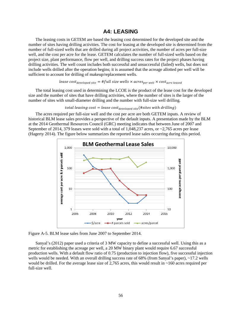
56

A4: LEASING The leasing costs in GETEM are based the leasing cost determined for the developed site and the

number of sites having drilling activities. The cost for leasing at the developed site is determined from the number of full-sized wells that are drilled during all project activities, the number of acres per full-size well, and the cost per acre for the lease. GETEM calculates the number of full-sized wells based on the project size, plant performance, flow per well, and drilling success rates for the project phases having drilling activities. The well count includes both successful and unsuccessful (failed) wells, but does not include wells drilled after the operation begins; it is assumed that the acreage allotted per well will be sufficient to account for drilling of makeup/replacement wells.

𝑆𝑆𝑃𝑃𝑆𝑆𝑆𝑆𝑃𝑃 𝑃𝑃𝑃𝑃𝑆𝑆𝑃𝑃𝑓𝑓𝑛𝑛𝑎𝑎𝑛𝑛𝑓𝑓𝑔𝑔𝑝𝑝𝑛𝑛𝑓𝑓 𝑑𝑑𝑓𝑓𝑛𝑛𝑛𝑛 = #𝑓𝑓𝑃𝑃𝑆𝑆𝑆𝑆 𝑆𝑆𝑃𝑃𝑙𝑙𝑃𝑃 𝑃𝑃𝑃𝑃𝑆𝑆𝑆𝑆𝑆𝑆 × 𝑆𝑆𝑃𝑃𝑃𝑃𝑃𝑃𝑆𝑆𝑝𝑝𝑛𝑛𝑝𝑝 𝑤𝑤𝑛𝑛𝑓𝑓𝑓𝑓 × 𝑃𝑃𝑃𝑃𝑆𝑆𝑃𝑃𝑝𝑝𝑎𝑎𝑝𝑝𝑛𝑛 𝑓𝑓𝑛𝑛𝑝𝑝𝑑𝑑𝑛𝑛𝑓𝑓

The total leasing cost used in determining the LCOE is the product of the lease cost for the developed size and the number of sites that have drilling activities, where the number of sites is the larger of the number of sites with small-diameter drilling and the number with full-size well drilling.

𝑃𝑃𝑃𝑃𝑃𝑃𝑆𝑆𝑆𝑆 𝑆𝑆𝑃𝑃𝑆𝑆𝑆𝑆𝑃𝑃𝑃𝑃𝑃𝑃 𝑃𝑃𝑃𝑃𝑆𝑆𝑃𝑃 = 𝑆𝑆𝑃𝑃𝑆𝑆𝑆𝑆𝑃𝑃 𝑃𝑃𝑃𝑃𝑆𝑆𝑃𝑃𝑓𝑓𝑛𝑛𝑎𝑎𝑛𝑛𝑓𝑓𝑔𝑔𝑝𝑝𝑛𝑛𝑓𝑓 𝑑𝑑𝑓𝑓𝑛𝑛𝑛𝑛(#𝑆𝑆𝑃𝑃𝑃𝑃𝑃𝑃𝑆𝑆 𝑃𝑃𝑃𝑃𝑃𝑃ℎ 𝑑𝑑𝑃𝑃𝑃𝑃𝑆𝑆𝑆𝑆𝑃𝑃𝑃𝑃𝑃𝑃)

The acres required per full-size well and the cost per acre are both GETEM inputs. A review of historical BLM lease sales provides a perspective of the default inputs. A presentation made by the BLM at the 2014 Geothermal Resources Council (GRC) meeting indicates that between June of 2007 and September of 2014, 379 leases were sold with a total of 1,048,237 acres, or ~2,765 acres per lease (Hagerty 2014). The figure below summarizes the reported lease sales occurring during this period.

Figure A-5. BLM lease sales from June 2007 to September 2014.

Sanyal’s (2012) paper used a criteria of 3 MW capacity to define a successful well. Using this as a metric for establishing the acreage per well, a 20 MW binary plant would require 6.67 successful production wells. With a default flow ratio of 0.75 (production to injection flow), five successful injection wells would be needed. With an overall drilling success rate of 68% (from Sanyal’s paper), ~17.2 wells would be drilled. For the average lease size of 2,765 acres, this would result in ~160 acres required per full-size well.

57

GETEM typically calculates a plant performance that results in a well capacity greater than 3 MW per well; for binary plants, the value is typically in the range of 4 to 5 MW capacity per well. Using a value of 4 MW capacity per well, the well count would be ~12.9 wells, or ~215 acres per full-size well for the average parcel size leased.

GETEM defaults to an average spacing of 0.75 km between well and plant. Assuming the wells were laid out with a similar spacing between wells, there would be ~110 acres per well. With this spacing, GETEM’s default value of 225 acres per well allows the well field to be replaced with this idealized well configuration.

The default lease cost of $30 per acre was established by the LCOE analysis team review of GETEM inputs in 2012, and was based on successful bids for the 2009 lease sale in Nevada. Though recent successful bids are lower, the default is considered representative of a cost during a period when geothermal energy production is expanding.

58

A5: WELL COUNT Hydrothermal Resources

Exploration Phase • There is no specific well count for slim holes, core holes, and/or temperature gradient holes. The costs

for those wells/holes are included in the lump sum value inputted.

• The default scenario assumes full-sized wells are drilled only at the site developed, but it can be revised to include drilling of full-sized wells at more than one site. If this is done, the user must identify how many wells are drilled at each unsuccessful site. (The default is 0 because the default only considers costs for the successful site.) Though costs for full-sized wells that are drilled at sites not developed may be included in the total exploration phase costs, these wells do not support the subsequent operation of a power plant.

• The model assumes that two successful full-sized wells are drilled during the exploration phase (at the final site developed). The model also assumes that to get a successful well, two wells must be drilled (based on a success rate of 50%). The default is that 2 × 2 or four full-sized wells are drilled during the exploration phase at the final site. Successful full-size exploration wells support plant operation.

Drilling Phase • The model assumes that drilling occurs only at the final site.

• Successful wells from the exploration phase are assumed to be production wells.

• If the user defines the project based on the number of production wells used, the number of successful production wells drilled during this phase is that defined number less the number of successful exploration wells.

• If the user defines the project based on power sales, the number of production wells required or needed is determined with the following relationships:

𝑃𝑃𝑃𝑃𝑃𝑃𝑆𝑆𝑆𝑆 𝐺𝐺𝐶𝐶 𝑓𝑓𝑆𝑆𝑃𝑃𝑃𝑃𝑝𝑝𝑛𝑛𝑟𝑟 =𝑃𝑃𝑃𝑃𝑃𝑃𝑃𝑃𝑃𝑃 𝑆𝑆𝑆𝑆𝑆𝑆𝑃𝑃𝑆𝑆

[𝑏𝑏𝑃𝑃𝑃𝑃𝑃𝑃𝑃𝑃 𝑃𝑃𝑓𝑓𝑓𝑓𝑃𝑃𝑃𝑃𝑃𝑃𝑃𝑃𝑙𝑙𝑃𝑃𝑃𝑃𝑃𝑃𝑆𝑆𝑆𝑆 − 𝐺𝐺𝐶𝐶 𝑃𝑃𝑃𝑃𝑃𝑃𝑃𝑃𝑃𝑃𝑃𝑃𝑃𝑃]

In this relationship, the brine effectiveness and GF pumping are in units of power per unit mass flow. The brine effectiveness is the numerator in the second law efficiency, and is the parameter that GETEM varies when determining the minimum LCOE. The GF pumping is based on the production and injection well flow rates, well depth, well injectivity or productivity, and the default casing design for each well type.

𝑃𝑃𝑃𝑃𝑃𝑃𝑑𝑑𝑃𝑃𝑃𝑃𝑃𝑃𝑃𝑃𝑃𝑃𝑃𝑃 𝑃𝑃𝑃𝑃𝑆𝑆𝑆𝑆𝑆𝑆𝑝𝑝𝑛𝑛𝑟𝑟 =𝑃𝑃𝑃𝑃𝑃𝑃𝑆𝑆𝑆𝑆 𝐺𝐺𝐶𝐶 𝑓𝑓𝑆𝑆𝑃𝑃𝑃𝑃𝑝𝑝𝑛𝑛𝑟𝑟𝑓𝑓𝑆𝑆𝑃𝑃𝑃𝑃𝑝𝑝𝑝𝑝𝑔𝑔𝑓𝑓 𝑤𝑤𝑛𝑛𝑓𝑓𝑓𝑓

The flow per production well is a model input that can be revised.

The number of production wells required is determined in this manner regardless of the type of resource or conversion system. Note that the number of wells required is based on the assumption that all wells have the same performance—temperature, flow rate, and productivity index.

• The number of injection wells required is also based on the total GF flow. A model variable is the ratio of the production well flow relative to the injection well flow.

𝑓𝑓𝑆𝑆𝑃𝑃𝑃𝑃𝑓𝑓𝑛𝑛𝑝𝑝𝑛𝑛𝑎𝑎𝑛𝑛 𝑤𝑤𝑛𝑛𝑓𝑓𝑓𝑓 =𝑓𝑓𝑆𝑆𝑃𝑃𝑃𝑃𝑝𝑝𝑝𝑝𝑔𝑔𝑓𝑓 𝑤𝑤𝑛𝑛𝑓𝑓𝑓𝑓

𝑃𝑃𝑆𝑆𝑃𝑃𝑃𝑃𝑃𝑃 𝑃𝑃𝑓𝑓 𝑃𝑃𝑃𝑃𝑃𝑃𝑑𝑑𝑃𝑃𝑃𝑃𝑃𝑃𝑃𝑃𝑃𝑃𝑃𝑃 𝑃𝑃𝑃𝑃 𝑃𝑃𝑃𝑃𝑝𝑝𝑃𝑃𝑃𝑃𝑃𝑃𝑃𝑃𝑃𝑃𝑃𝑃 𝑃𝑃𝑃𝑃𝑆𝑆𝑆𝑆 𝑓𝑓𝑆𝑆𝑃𝑃𝑃𝑃

𝑃𝑃𝑃𝑃𝑝𝑝𝑃𝑃𝑃𝑃𝑃𝑃𝑃𝑃𝑃𝑃𝑃𝑃 𝑃𝑃𝑃𝑃𝑆𝑆𝑆𝑆𝑆𝑆𝑝𝑝𝑛𝑛𝑟𝑟 =𝑃𝑃𝑃𝑃𝑃𝑃𝑆𝑆𝑆𝑆 𝐺𝐺𝐶𝐶 𝑓𝑓𝑆𝑆𝑃𝑃𝑃𝑃𝑓𝑓𝑛𝑛𝑝𝑝𝑛𝑛𝑎𝑎𝑛𝑛𝑛𝑛𝑓𝑓

𝑓𝑓𝑆𝑆𝑃𝑃𝑃𝑃𝑓𝑓𝑛𝑛𝑝𝑝𝑛𝑛𝑎𝑎𝑛𝑛 𝑤𝑤𝑛𝑛𝑓𝑓𝑓𝑓

59

With flash power plants, the total flow injected will be less than the total flow produced, unless the water loss in the evaporative cooling towers is made up. Making up this loss is an option for hydrothermal resources, for which sufficient makeup is provided that injected flow and produced flow are equivalent.

These relationships are the basis for determining the number of injection wells required when failed wells are not used to supplement injection flow. Whether or not to use failed wells is a model variable for hydrothermal resources. This model variable is not used for EGS or hydrothermal resources for which wells are stimulated. If failed wells are used, then all failed production and injection wells are used. The method for determining the number of “successful” injection wells is described below.

• Use of Failed Wells:

- Failed wells are assumed to have a productivity relative to successful wells (a value less than 1). This is a model input that can be revised. The injectivity index of a failed well (𝐼𝐼𝐼𝐼𝑓𝑓𝑝𝑝𝑓𝑓𝑓𝑓_𝑤𝑤𝑛𝑛𝑓𝑓𝑓𝑓) is

𝐼𝐼𝐼𝐼𝑓𝑓𝑝𝑝𝑓𝑓𝑓𝑓_𝑤𝑤𝑛𝑛𝑓𝑓𝑓𝑓 = 𝑃𝑃𝑃𝑃𝑃𝑃𝑑𝑑𝑃𝑃𝑃𝑃𝑃𝑃𝑃𝑃𝑙𝑙𝑃𝑃𝑃𝑃𝑐𝑐 𝐼𝐼𝑃𝑃𝑑𝑑𝑃𝑃𝐼𝐼𝑑𝑑𝑓𝑓𝑎𝑎𝑎𝑎𝑛𝑛𝑑𝑑𝑑𝑑𝑓𝑓𝑓𝑓𝑓𝑓_𝑤𝑤𝑛𝑛𝑓𝑓𝑓𝑓 × 𝑃𝑃𝑃𝑃𝑆𝑆𝑆𝑆𝑃𝑃𝑃𝑃𝑙𝑙𝑃𝑃 𝑃𝑃𝑃𝑃𝑃𝑃𝑑𝑑𝑃𝑃𝑃𝑃𝑃𝑃𝑃𝑃𝑙𝑙𝑃𝑃𝑃𝑃𝑐𝑐 - The injection flow taken by a failed production well is estimated as:

𝑓𝑓𝑆𝑆𝑃𝑃𝑃𝑃𝑓𝑓𝑝𝑝𝑓𝑓𝑓𝑓_𝑃𝑃𝑘𝑘 = �𝑃𝑃𝑤𝑤𝑛𝑛𝑓𝑓𝑓𝑓−ℎ𝑛𝑛𝑝𝑝𝑓𝑓 + ∆𝑃𝑃𝑓𝑓𝑛𝑛𝑝𝑝_𝑝𝑝𝑓𝑓𝑝𝑝𝑝𝑝 + 𝜌𝜌𝑓𝑓𝑛𝑛𝑝𝑝(𝑑𝑑𝑃𝑃𝑃𝑃𝑃𝑃ℎ𝑃𝑃𝑘𝑘) − ∆𝑃𝑃𝑓𝑓𝑝𝑝𝑓𝑓𝑎𝑎𝑛𝑛𝑓𝑓𝑔𝑔𝑛𝑛 − 𝑃𝑃ℎ𝑎𝑎𝑓𝑓𝑝𝑝𝑔𝑔𝑑𝑑𝑛𝑛𝑝𝑝𝑛𝑛𝑓𝑓𝑎𝑎� × 𝐼𝐼𝐼𝐼𝑓𝑓𝑝𝑝𝑓𝑓𝑓𝑓_𝑤𝑤𝑛𝑛𝑓𝑓𝑓𝑓 This calculation is based upon the injection pump head determined for the flow in a successful

injection well. In this relationship, GETEM estimates the friction loss (ΔPfriction) based on that determined for a successful well, with the assumption that the flow will be proportional to the relative productivity specified.

- A similar approach is used to determine the flow in the failed injection wells that are used to supplement total injection. The primary difference is that instead of the production well depth, the injection well depth is used to determine flow rate in those wells.

- The number of injection wells that are drilled is based on the total flow to the injection wells: 𝑃𝑃𝑃𝑃𝑃𝑃𝑆𝑆𝑆𝑆 𝑓𝑓𝑆𝑆𝑃𝑃𝑃𝑃𝐼𝐼𝑘𝑘 = 𝑃𝑃𝑃𝑃𝑃𝑃𝑆𝑆𝑆𝑆 𝐺𝐺𝐶𝐶 𝑓𝑓𝑆𝑆𝑃𝑃𝑃𝑃 − #𝑃𝑃𝑃𝑃𝑓𝑓𝑝𝑝𝑓𝑓𝑓𝑓�𝑓𝑓𝑆𝑆𝑃𝑃𝑃𝑃𝑓𝑓𝑝𝑝𝑓𝑓𝑓𝑓_𝑃𝑃𝑃𝑃�

𝑃𝑃𝑃𝑃𝑃𝑃𝑆𝑆𝑆𝑆 𝑓𝑓𝑆𝑆𝑃𝑃𝑃𝑃𝐼𝐼𝑘𝑘 = #𝐼𝐼𝑃𝑃𝑑𝑑𝑓𝑓𝑎𝑎�𝑓𝑓𝑆𝑆𝑃𝑃𝑃𝑃𝑑𝑑𝑓𝑓𝑎𝑎𝑎𝑎𝑛𝑛𝑑𝑑𝑑𝑑𝑓𝑓𝑓𝑓𝑓𝑓_𝐼𝐼𝑘𝑘� + #𝐼𝐼𝑃𝑃𝑓𝑓𝑝𝑝𝑓𝑓𝑓𝑓�𝑓𝑓𝑆𝑆𝑃𝑃𝑃𝑃𝑓𝑓𝑝𝑝𝑓𝑓𝑓𝑓_𝑖𝑖𝑃𝑃� - These relationships can be used to determine the number of successful injection wells that must

be drilled based on the inputted drilling success rate (DSR): #𝐼𝐼𝑃𝑃𝑑𝑑𝑓𝑓𝑎𝑎 = #𝐼𝐼𝑃𝑃𝑓𝑓𝑝𝑝𝑓𝑓𝑓𝑓𝑓𝑓𝑛𝑛𝑓𝑓(𝐷𝐷𝑆𝑆𝑅𝑅)

#𝐼𝐼𝑃𝑃𝑓𝑓𝑝𝑝𝑓𝑓𝑓𝑓 = #𝐼𝐼𝑃𝑃𝑓𝑓𝑝𝑝𝑓𝑓𝑓𝑓𝑓𝑓𝑛𝑛𝑓𝑓(1 − 𝐷𝐷𝑆𝑆𝑅𝑅)

#𝐼𝐼𝑃𝑃𝑓𝑓𝑝𝑝𝑓𝑓𝑓𝑓 = #𝐼𝐼𝑃𝑃𝑑𝑑𝑓𝑓𝑎𝑎 �1

𝐷𝐷𝑆𝑆𝑅𝑅− 1�

#𝑃𝑃𝑃𝑃𝑓𝑓𝑝𝑝𝑓𝑓𝑓𝑓 = #𝑃𝑃𝑃𝑃𝑑𝑑𝑓𝑓𝑎𝑎 �1

𝐷𝐷𝑆𝑆𝑅𝑅− 1�

𝑃𝑃𝑃𝑃𝑃𝑃𝑆𝑆𝑆𝑆 𝑓𝑓𝑆𝑆𝑃𝑃𝑃𝑃𝐼𝐼𝑘𝑘 = #𝐼𝐼𝑃𝑃𝑑𝑑𝑓𝑓𝑎𝑎 �𝑓𝑓𝑆𝑆𝑃𝑃𝑃𝑃𝑑𝑑𝑓𝑓𝑎𝑎_𝐼𝐼𝑘𝑘 + 𝑓𝑓𝑆𝑆𝑃𝑃𝑃𝑃𝑓𝑓𝑝𝑝𝑓𝑓𝑓𝑓_𝐼𝐼𝑘𝑘 �1

𝐷𝐷𝑆𝑆𝑅𝑅− 1��

#𝐼𝐼𝑃𝑃𝑑𝑑𝑓𝑓𝑎𝑎 =𝑃𝑃𝑃𝑃𝑃𝑃𝑆𝑆𝑆𝑆 𝑓𝑓𝑆𝑆𝑃𝑃𝑃𝑃𝐼𝐼𝑘𝑘

�𝑓𝑓𝑆𝑆𝑃𝑃𝑃𝑃𝑑𝑑𝑓𝑓𝑎𝑎_𝐼𝐼𝑘𝑘 + 𝑓𝑓𝑆𝑆𝑃𝑃𝑃𝑃𝑓𝑓𝑝𝑝𝑓𝑓𝑓𝑓_𝐼𝐼𝑘𝑘 � 1𝐷𝐷𝑆𝑆𝑅𝑅 − 1��

#𝐼𝐼𝑃𝑃𝑑𝑑𝑓𝑓𝑎𝑎 =�𝑃𝑃𝑃𝑃𝑃𝑃𝑆𝑆𝑆𝑆 𝐺𝐺𝐶𝐶 𝑓𝑓𝑆𝑆𝑃𝑃𝑃𝑃 − #𝑃𝑃𝑃𝑃𝑓𝑓𝑝𝑝𝑓𝑓𝑓𝑓�𝑓𝑓𝑆𝑆𝑃𝑃𝑃𝑃𝑓𝑓𝑝𝑝𝑓𝑓𝑓𝑓_𝑃𝑃𝑃𝑃��

�𝑓𝑓𝑆𝑆𝑃𝑃𝑃𝑃𝑑𝑑𝑓𝑓𝑎𝑎_𝐼𝐼𝑘𝑘 + 𝑓𝑓𝑆𝑆𝑃𝑃𝑃𝑃𝑓𝑓𝑝𝑝𝑓𝑓𝑓𝑓_𝐼𝐼𝑘𝑘 � 1𝐷𝐷𝑆𝑆𝑅𝑅 − 1��

In this relationship, the number of failed production wells is based on the number of production wells needed or required (#𝑃𝑃𝑃𝑃𝑑𝑑𝑓𝑓𝑎𝑎).

• Total Wells Drilled During Drilling Phase—Hydrothermal Resources

- The total number of production wells drilled is calculated as follows:

𝑃𝑃𝑃𝑃𝑃𝑃𝑑𝑑𝑃𝑃𝑃𝑃𝑃𝑃𝑃𝑃𝑃𝑃𝑃𝑃 𝑃𝑃𝑃𝑃𝑆𝑆𝑆𝑆𝑆𝑆𝑓𝑓𝑝𝑝𝑓𝑓𝑓𝑓𝑓𝑓𝑛𝑛𝑓𝑓 =�𝑃𝑃𝑃𝑃𝑃𝑃𝑑𝑑𝑃𝑃𝑃𝑃𝑃𝑃𝑃𝑃𝑃𝑃𝑃𝑃 𝑃𝑃𝑃𝑃𝑆𝑆𝑆𝑆𝑆𝑆𝑝𝑝𝑛𝑛𝑟𝑟 − # 𝑓𝑓𝑃𝑃𝑆𝑆𝑆𝑆 𝑆𝑆𝑃𝑃𝑙𝑙𝑃𝑃 𝑃𝑃𝐼𝐼𝑃𝑃𝑆𝑆 𝑃𝑃𝑃𝑃𝑆𝑆𝑆𝑆𝑑𝑑𝑓𝑓𝑎𝑎�

𝐷𝐷𝑆𝑆𝑅𝑅

60

𝑃𝑃𝑃𝑃𝑝𝑝𝑃𝑃𝑃𝑃𝑃𝑃𝑃𝑃𝑃𝑃𝑃𝑃 𝑃𝑃𝑃𝑃𝑆𝑆𝑆𝑆𝑆𝑆𝑓𝑓𝑝𝑝𝑓𝑓𝑓𝑓𝑓𝑓𝑛𝑛𝑓𝑓 =�𝑃𝑃𝑃𝑃𝑝𝑝𝑃𝑃𝑃𝑃𝑃𝑃𝑃𝑃𝑃𝑃𝑃𝑃 𝑃𝑃𝑃𝑃𝑆𝑆𝑆𝑆𝑆𝑆𝑝𝑝𝑛𝑛𝑟𝑟�

𝐷𝐷𝑆𝑆𝑅𝑅

where

𝑃𝑃𝑃𝑃𝑃𝑃𝑑𝑑𝑃𝑃𝑃𝑃𝑃𝑃𝑃𝑃𝑃𝑃𝑃𝑃 𝑃𝑃𝑃𝑃𝑆𝑆𝑆𝑆𝑆𝑆𝑝𝑝𝑛𝑛𝑟𝑟 =𝑃𝑃𝑃𝑃𝑃𝑃𝑆𝑆𝑆𝑆 𝐺𝐺𝐶𝐶 𝑓𝑓𝑆𝑆𝑃𝑃𝑃𝑃𝑝𝑝𝑛𝑛𝑟𝑟𝑓𝑓𝑆𝑆𝑃𝑃𝑃𝑃𝑝𝑝𝑝𝑝𝑔𝑔𝑓𝑓 𝑤𝑤𝑛𝑛𝑓𝑓𝑓𝑓

If failed wells are not used to supplement injection, the number of injection wells required is

𝑃𝑃𝑃𝑃𝑝𝑝𝑃𝑃𝑃𝑃𝑃𝑃𝑃𝑃𝑃𝑃𝑃𝑃 𝑃𝑃𝑃𝑃𝑆𝑆𝑆𝑆𝑆𝑆𝑝𝑝𝑛𝑛𝑟𝑟 =𝑃𝑃𝑃𝑃𝑃𝑃𝑆𝑆𝑆𝑆 𝐺𝐺𝐶𝐶 𝑓𝑓𝑆𝑆𝑃𝑃𝑃𝑃𝑝𝑝𝑛𝑛𝑟𝑟𝑓𝑓𝑆𝑆𝑃𝑃𝑃𝑃𝑓𝑓𝑛𝑛𝑝𝑝𝑛𝑛𝑎𝑎𝑛𝑛 𝑤𝑤𝑛𝑛𝑓𝑓𝑓𝑓

or when failed wells are used, the number of successful injection wells needed is

#𝐼𝐼𝑃𝑃𝑑𝑑𝑓𝑓𝑎𝑎 =�𝑃𝑃𝑃𝑃𝑃𝑃𝑆𝑆𝑆𝑆 𝐺𝐺𝐶𝐶 𝑓𝑓𝑆𝑆𝑃𝑃𝑃𝑃 − #𝑃𝑃𝑃𝑃𝑓𝑓𝑝𝑝𝑓𝑓𝑓𝑓�𝑓𝑓𝑆𝑆𝑃𝑃𝑃𝑃𝑓𝑓𝑝𝑝𝑓𝑓𝑓𝑓_𝑃𝑃𝑃𝑃��

�𝑓𝑓𝑆𝑆𝑃𝑃𝑃𝑃𝑑𝑑𝑓𝑓𝑎𝑎_𝐼𝐼𝑘𝑘 + 𝑓𝑓𝑆𝑆𝑃𝑃𝑃𝑃𝑓𝑓𝑝𝑝𝑓𝑓𝑓𝑓_𝐼𝐼𝑘𝑘 � 1𝐷𝐷𝑆𝑆𝑅𝑅 − 1��

where #𝐼𝐼𝑃𝑃𝑑𝑑𝑓𝑓𝑎𝑎 = 𝑃𝑃𝑃𝑃𝑝𝑝𝑃𝑃𝑃𝑃𝑃𝑃𝑃𝑃𝑃𝑃𝑃𝑃 𝑃𝑃𝑃𝑃𝑆𝑆𝑆𝑆𝑆𝑆𝑝𝑝𝑛𝑛𝑟𝑟

The use of all failed wells to support the operation of the power plant is the current GETEM default for hydrothermal resources. This version of GETEM differs from previous versions in that the user defines the ratio of production to injection flow rate for successful wells. Previously, a user inputted the ratio of injection to production wells, and that ratio was used to determine the number of injection wells drilled. If one opts not to use failed wells to supplement injection, the model’s calculations will reflect the previous approach used—unless the hydrothermal wells are stimulated.

The current version of GETEM has modified the use of stimulation for hydrothermal resources. If wells are stimulated with hydrothermal resources, then only failed wells in the Drilling phase are stimulated. If stimulation is specified, it can be applied to failed production, failed injection, or both well types. A stimulation success rate (SSR) is applied to reflect that not all stimulations are successful. A successfully stimulated well will perform equivalent to a successfully drilled well. When wells are stimulated, the option to used failed wells to supplement injection is not used, regardless of the input provided. This occurs even for those failed wells that are not stimulated (if one opts to only stimulate either production or injection wells). It also applies to wells that are unsuccessfully stimulated.

• Hydrothermal Well Stimulation

- If production wells are stimulated, the number of production wells drilled during the Drilling phase can be determined using the following. (Note in these equations that SSR is the stimulation success rate.)

#𝑃𝑃𝑃𝑃𝑑𝑑𝑓𝑓𝑎𝑎 = 𝑃𝑃𝑃𝑃𝑃𝑃𝑑𝑑𝑃𝑃𝑃𝑃𝑃𝑃𝑃𝑃𝑃𝑃𝑃𝑃 𝑃𝑃𝑃𝑃𝑆𝑆𝑆𝑆𝑝𝑝𝑛𝑛𝑟𝑟 − #𝑓𝑓𝑃𝑃𝑆𝑆𝑆𝑆 𝑆𝑆𝑃𝑃𝑙𝑙𝑃𝑃 𝐿𝐿𝐼𝐼𝑃𝑃𝑆𝑆 𝑃𝑃𝑃𝑃𝑆𝑆𝑆𝑆𝑑𝑑𝑓𝑓𝑎𝑎 #𝑃𝑃𝑃𝑃𝑑𝑑𝑓𝑓𝑎𝑎 = #𝑃𝑃𝑃𝑃𝑓𝑓𝑝𝑝𝑓𝑓𝑓𝑓𝑓𝑓𝑛𝑛𝑓𝑓 − #𝑃𝑃𝑃𝑃𝑓𝑓𝑝𝑝𝑓𝑓𝑓𝑓_𝑓𝑓𝑝𝑝𝑓𝑓𝑓𝑓𝑓𝑓&𝑆𝑆𝑛𝑛𝑓𝑓𝑝𝑝 #𝑃𝑃𝑃𝑃𝑓𝑓𝑝𝑝𝑓𝑓𝑓𝑓𝑓𝑓𝑛𝑛𝑓𝑓 = #𝑃𝑃𝑃𝑃𝑑𝑑𝑓𝑓𝑎𝑎_𝑓𝑓𝑝𝑝𝑓𝑓𝑓𝑓𝑓𝑓 + #𝑃𝑃𝑃𝑃𝑓𝑓𝑝𝑝𝑓𝑓𝑓𝑓_𝑓𝑓𝑝𝑝𝑓𝑓𝑓𝑓𝑓𝑓

#𝑃𝑃𝑃𝑃𝑑𝑑𝑓𝑓𝑎𝑎_𝑓𝑓𝑝𝑝𝑓𝑓𝑓𝑓𝑓𝑓 = #𝑃𝑃𝑃𝑃𝑓𝑓𝑝𝑝𝑓𝑓𝑓𝑓𝑓𝑓𝑛𝑛𝑓𝑓 × 𝐷𝐷𝑆𝑆𝑅𝑅 #𝑃𝑃𝑃𝑃𝑓𝑓𝑝𝑝𝑓𝑓𝑓𝑓_𝑓𝑓𝑝𝑝𝑓𝑓𝑓𝑓𝑓𝑓 = #𝑃𝑃𝑃𝑃𝑓𝑓𝑝𝑝𝑓𝑓𝑓𝑓𝑓𝑓𝑛𝑛𝑓𝑓 × (1 − 𝐷𝐷𝑆𝑆𝑅𝑅)

#𝑃𝑃𝑃𝑃𝑓𝑓𝑝𝑝𝑓𝑓𝑓𝑓_𝑓𝑓𝑝𝑝𝑓𝑓𝑓𝑓𝑓𝑓&𝑆𝑆𝑛𝑛𝑓𝑓𝑝𝑝 = (1 − 𝑆𝑆𝑆𝑆𝑅𝑅)#𝑃𝑃𝑃𝑃𝑓𝑓𝑝𝑝𝑓𝑓𝑓𝑓_𝑓𝑓𝑝𝑝𝑓𝑓𝑓𝑓𝑓𝑓 #𝑃𝑃𝑃𝑃𝑑𝑑𝑓𝑓𝑎𝑎 = #𝑃𝑃𝑃𝑃𝑑𝑑𝑓𝑓𝑎𝑎_𝑓𝑓𝑝𝑝𝑓𝑓𝑓𝑓𝑓𝑓 + #𝑃𝑃𝑃𝑃𝑓𝑓𝑝𝑝𝑓𝑓𝑓𝑓_𝑓𝑓𝑝𝑝𝑓𝑓𝑓𝑓𝑓𝑓 − #𝑃𝑃𝑃𝑃𝑓𝑓𝑝𝑝𝑓𝑓𝑓𝑓 _𝑓𝑓𝑝𝑝𝑓𝑓𝑓𝑓𝑓𝑓&𝑑𝑑𝑛𝑛𝑓𝑓𝑝𝑝

#𝑃𝑃𝑃𝑃𝑑𝑑𝑓𝑓𝑎𝑎 = #𝑃𝑃𝑃𝑃𝑓𝑓𝑝𝑝𝑓𝑓𝑓𝑓𝑓𝑓𝑛𝑛𝑓𝑓 × 𝐷𝐷𝑆𝑆𝑅𝑅 + #𝑃𝑃𝑃𝑃𝑓𝑓𝑝𝑝𝑓𝑓𝑓𝑓𝑓𝑓𝑛𝑛𝑓𝑓(1 − 𝐷𝐷𝑆𝑆𝑅𝑅) − #𝑃𝑃𝑃𝑃𝑓𝑓𝑝𝑝𝑓𝑓𝑓𝑓𝑓𝑓𝑛𝑛𝑓𝑓(1 − 𝑆𝑆𝑆𝑆𝑅𝑅)(1 − 𝐷𝐷𝑆𝑆𝑅𝑅) #𝑃𝑃𝑃𝑃𝑑𝑑𝑓𝑓𝑎𝑎 = #𝑃𝑃𝑃𝑃𝑓𝑓𝑝𝑝𝑓𝑓𝑓𝑓𝑓𝑓𝑛𝑛𝑓𝑓[𝐷𝐷𝑆𝑆𝑅𝑅 + (1 − 𝐷𝐷𝑆𝑆𝑅𝑅) − (1 − 𝑆𝑆𝑆𝑆𝑅𝑅)(1 − 𝐷𝐷𝑆𝑆𝑅𝑅)]

#𝑃𝑃𝑃𝑃𝑑𝑑𝑓𝑓𝑎𝑎 = #𝑃𝑃𝑃𝑃𝑓𝑓𝑝𝑝𝑓𝑓𝑓𝑓𝑓𝑓𝑛𝑛𝑓𝑓[1 − (1 − 𝑆𝑆𝑆𝑆𝑅𝑅)(1 − 𝐷𝐷𝑆𝑆𝑅𝑅)]

#𝑃𝑃𝑃𝑃𝑓𝑓𝑝𝑝𝑓𝑓𝑓𝑓𝑓𝑓𝑛𝑛𝑓𝑓 =#𝑃𝑃𝑃𝑃𝑑𝑑𝑓𝑓𝑎𝑎

[1 − (1 − 𝑆𝑆𝑆𝑆𝑅𝑅)(1 − 𝐷𝐷𝑆𝑆𝑅𝑅)]

#𝑃𝑃𝑃𝑃𝑓𝑓𝑝𝑝𝑓𝑓𝑓𝑓𝑓𝑓𝑛𝑛𝑓𝑓 =�𝑃𝑃𝑃𝑃𝑃𝑃𝑑𝑑𝑃𝑃𝑃𝑃𝑃𝑃𝑃𝑃𝑃𝑃𝑃𝑃 𝑃𝑃𝑃𝑃𝑆𝑆𝑆𝑆𝑝𝑝𝑛𝑛𝑟𝑟 − #𝑓𝑓𝑃𝑃𝑆𝑆𝑆𝑆 𝑆𝑆𝑃𝑃𝑙𝑙𝑃𝑃 𝐿𝐿𝐼𝐼𝑃𝑃𝑆𝑆 𝑃𝑃𝑃𝑃𝑆𝑆𝑆𝑆𝑑𝑑𝑓𝑓𝑎𝑎�

[1 − (1 − 𝑆𝑆𝑆𝑆𝑅𝑅)(1 − 𝐷𝐷𝑆𝑆𝑅𝑅)]

61

- A similar approach is used to determine the number of injection wells drilled when they are stimulated. In this case, the number of successful wells used for injection is 0. The number of injection wells required is:

𝑃𝑃𝑃𝑃𝑝𝑝𝑃𝑃𝑃𝑃𝑃𝑃𝑃𝑃𝑃𝑃𝑃𝑃 𝑃𝑃𝑃𝑃𝑆𝑆𝑆𝑆𝑆𝑆𝑝𝑝𝑛𝑛𝑟𝑟 =𝑃𝑃𝑃𝑃𝑃𝑃𝑆𝑆𝑆𝑆 𝐺𝐺𝐶𝐶 𝑓𝑓𝑆𝑆𝑃𝑃𝑃𝑃𝑝𝑝𝑛𝑛𝑟𝑟𝑓𝑓𝑆𝑆𝑃𝑃𝑃𝑃𝑓𝑓𝑛𝑛𝑝𝑝𝑛𝑛𝑎𝑎𝑛𝑛 𝑤𝑤𝑛𝑛𝑓𝑓𝑓𝑓

#𝐼𝐼𝑃𝑃𝑓𝑓𝑝𝑝𝑓𝑓𝑓𝑓𝑓𝑓𝑛𝑛𝑓𝑓 =� 𝑃𝑃𝑃𝑃𝑝𝑝𝑃𝑃𝑃𝑃𝑃𝑃𝑃𝑃𝑃𝑃𝑃𝑃 𝑃𝑃𝑃𝑃𝑆𝑆𝑆𝑆𝑝𝑝𝑛𝑛𝑟𝑟�

[1 − (1 − 𝑆𝑆𝑆𝑆𝑅𝑅)(1 − 𝐷𝐷𝑆𝑆𝑅𝑅)]

• The model default for the drilling success rate is 75% during the Drilling phase. Some of the values the model uses as defaults are best estimates. For hydrothermal resources these values include:

- Productivity of unsuccessful wells relative to successful wells: 0.30 - SSR: 75% - Stimulation costs: $2,500,000 (This value is from the work done in 2012. It is brought forward in

time using the Bureau of Labor Statistics PPI for drilling services.)

EGS Resources Exploration Phase

An approach similar to that used for hydrothermal resources is used to determine the exploration well count with EGS resources. The number of wells drilled to get a successful well is still an input used to determine the total number of wells drilled. For an EGS resource, it is assumed that one of the wells drilled is also successfully stimulated; this assumption is inherent to the model and cannot be revised. GETEM has input for the number of wells to be stimulated during the exploration phase; the stimulation success rate during exploration is effectively this inverse of this input.

GETEM’s default is that three wells from the exploration phase will be considered successful and utilized to support the operation of the power plant; one of these wells will be successfully stimulated. GETEM’s EGS defaults are that there will be one stimulation failure, that two wells are drilled to get a successful well, and that injection wells will be stimulated.

Using these defaults to achieve three successful wells, six full-sized well are drilled. One of the three unsuccessful wells will be stimulated, as well as one of the successful wells. Of the three successful wells, one will be an injection well (stimulated) and the other two will be production wells.

As with hydrothermal resources, the costs to drill both the unsuccessful and successful full-sized wells are included in the exploration costs. With EGS resources, exploration costs also include the stimulation costs for the number of wells specified as being stimulated. If one opts to stimulate only production wells, then one of the three successful wells will be a production well (successfully stimulated), and the remainder will be injection wells. If both wells are stimulated, then all successful wells from the exploration phase will be successfully stimulated, with the total evenly split between production and injection. In this case, though multiple wells may be successfully stimulated, the default assumption remains that one stimulation is a failure.

If the stimulated wells are injection wells, and if the number of successful exploration wells is two or more, then

- # exploration wells used for injection = 1 - # exploration wells used for production = # successful exploration wells – 1 If 1 < # successful exploration wells < 2, then

- # exploration wells used for injection = 1 - # exploration wells used for production = # successful exploration wells – 1 If # successful exploration wells < 1, then

62

- # exploration wells used for injection = # successful exploration wells - # exploration wells used for production = 0 If the stimulated wells are production wells, and if the number of successful exploration wells is two

or more, then

- # exploration wells used for injection = # successful exploration wells – 1 - # exploration wells used for production = 1 If 1 < # successful exploration wells < 2, then

- # exploration wells used for injection = # successful exploration wells – 1 - # exploration wells used for production = 1 If # successful exploration wells < 1, then

- # exploration wells used for injection = 0 - # exploration wells used for production = # successful exploration wells If both production and injection wells are stimulated, then

- ½ of the successful # exploration wells are used for injection - ½ of the successful # exploration wells are used for production

Drilling Phase The determination of the number of successful production and injection wells required is the same as

that used for the hydrothermal resource:

𝑃𝑃𝑃𝑃𝑃𝑃𝑑𝑑𝑃𝑃𝑃𝑃𝑃𝑃𝑃𝑃𝑃𝑃𝑃𝑃 𝑃𝑃𝑃𝑃𝑆𝑆𝑆𝑆𝑆𝑆𝑝𝑝𝑛𝑛𝑟𝑟 =𝑃𝑃𝑃𝑃𝑃𝑃𝑆𝑆𝑆𝑆 𝐺𝐺𝐶𝐶 𝑓𝑓𝑆𝑆𝑃𝑃𝑃𝑃𝑝𝑝𝑛𝑛𝑟𝑟𝑓𝑓𝑆𝑆𝑃𝑃𝑃𝑃𝑝𝑝𝑝𝑝𝑔𝑔𝑓𝑓 𝑤𝑤𝑛𝑛𝑓𝑓𝑓𝑓

𝑃𝑃𝑃𝑃𝑝𝑝𝑃𝑃𝑃𝑃𝑃𝑃𝑃𝑃𝑃𝑃𝑃𝑃 𝑃𝑃𝑃𝑃𝑆𝑆𝑆𝑆𝑆𝑆𝑝𝑝𝑛𝑛𝑟𝑟 =𝑃𝑃𝑃𝑃𝑃𝑃𝑆𝑆𝑆𝑆 𝐺𝐺𝐶𝐶 𝑓𝑓𝑆𝑆𝑃𝑃𝑃𝑃𝑓𝑓𝑛𝑛𝑝𝑝𝑛𝑛𝑎𝑎𝑛𝑛𝑛𝑛𝑓𝑓

𝑓𝑓𝑆𝑆𝑃𝑃𝑃𝑃𝑓𝑓𝑛𝑛𝑝𝑝𝑛𝑛𝑎𝑎𝑛𝑛 𝑤𝑤𝑛𝑛𝑓𝑓𝑓𝑓

With EGS resources, the amount of fluid injected is equal to the total flow produced plus makeup for any specified subsurface losses. It is assumed that failed EGS wells will not be used to supplement injection, and it is assumed that if a well stimulation fails, the well will not be used.

GETEM allows for the injection wells only to be stimulated (model default), the production wells only to be stimulated, or for both injection and production wells to be stimulated. In determining how many wells are drilled and stimulated in this phase, it is necessary to account for those successful wells that are drilled in the exploration phase.

• Injection Well Only Stimulated:

- The number of production wells drilled in this phase is based on the drilling success rate (DSR), the number of successful exploration wells that are considered to be production wells, and the number of production wells required.

𝑃𝑃𝑃𝑃𝑃𝑃𝑑𝑑𝑃𝑃𝑃𝑃𝑃𝑃𝑃𝑃𝑃𝑃𝑃𝑃 𝑃𝑃𝑃𝑃𝑆𝑆𝑆𝑆𝑆𝑆𝑓𝑓𝑝𝑝𝑓𝑓𝑓𝑓𝑓𝑓𝑛𝑛𝑓𝑓 =�𝑃𝑃𝑃𝑃𝑃𝑃𝑑𝑑𝑃𝑃𝑃𝑃𝑃𝑃𝑃𝑃𝑃𝑃𝑃𝑃 𝑃𝑃𝑃𝑃𝑆𝑆𝑆𝑆𝑆𝑆𝑝𝑝𝑛𝑛𝑟𝑟 − #𝐿𝐿𝐼𝐼𝑃𝑃 𝑃𝑃𝑃𝑃𝑆𝑆𝑆𝑆𝑆𝑆𝑑𝑑𝑓𝑓𝑎𝑎_𝑝𝑝𝑝𝑝𝑔𝑔𝑓𝑓 𝑤𝑤𝑛𝑛𝑓𝑓𝑓𝑓�

𝐷𝐷𝑆𝑆𝑅𝑅

- The number of injection wells drilled is based on the DSR, the SSR, the number of successful exploration wells considered to be injection wells, and the number of injection wells required.

𝑃𝑃𝑃𝑃𝑝𝑝𝑃𝑃𝑃𝑃𝑃𝑃𝑃𝑃𝑃𝑃𝑃𝑃 𝑃𝑃𝑃𝑃𝑆𝑆𝑆𝑆𝑆𝑆𝑓𝑓𝑝𝑝𝑓𝑓𝑓𝑓𝑓𝑓𝑛𝑛𝑓𝑓 =�𝑃𝑃𝑃𝑃𝑝𝑝𝑃𝑃𝑃𝑃𝑃𝑃𝑃𝑃𝑃𝑃𝑃𝑃 𝑃𝑃𝑃𝑃𝑆𝑆𝑆𝑆𝑆𝑆𝑝𝑝𝑛𝑛𝑟𝑟 − #𝐿𝐿𝐼𝐼𝑃𝑃 𝑃𝑃𝑃𝑃𝑆𝑆𝑆𝑆𝑆𝑆𝑑𝑑𝑓𝑓𝑎𝑎_𝑓𝑓𝑛𝑛𝑝𝑝𝑛𝑛𝑎𝑎𝑛𝑛 𝑤𝑤𝑛𝑛𝑓𝑓𝑓𝑓�

[𝐷𝐷𝑆𝑆𝑅𝑅 × 𝑆𝑆𝑆𝑆𝑅𝑅]

- The number of injection wells stimulated is based on the following: 𝑃𝑃𝑃𝑃𝑝𝑝𝑃𝑃𝑃𝑃𝑃𝑃𝑃𝑃𝑃𝑃𝑃𝑃 𝑃𝑃𝑃𝑃𝑆𝑆𝑆𝑆𝑆𝑆𝑑𝑑𝑛𝑛𝑓𝑓𝑝𝑝 = 𝑃𝑃𝑃𝑃𝑝𝑝𝑃𝑃𝑃𝑃𝑃𝑃𝑃𝑃𝑃𝑃𝑃𝑃 𝑃𝑃𝑃𝑃𝑆𝑆𝑆𝑆𝑆𝑆𝑓𝑓𝑝𝑝𝑓𝑓𝑓𝑓𝑓𝑓𝑛𝑛𝑓𝑓 × 𝐷𝐷𝑆𝑆𝑅𝑅

𝑃𝑃𝑃𝑃𝑝𝑝𝑃𝑃𝑃𝑃𝑃𝑃𝑃𝑃𝑃𝑃𝑃𝑃 𝑃𝑃𝑃𝑃𝑆𝑆𝑆𝑆𝑆𝑆𝑑𝑑𝑓𝑓𝑎𝑎_𝑑𝑑𝑛𝑛𝑓𝑓𝑝𝑝 = 𝑃𝑃𝑃𝑃𝑝𝑝𝑃𝑃𝑃𝑃𝑃𝑃𝑃𝑃𝑃𝑃𝑃𝑃 𝑃𝑃𝑃𝑃𝑆𝑆𝑆𝑆𝑆𝑆𝑑𝑑𝑛𝑛𝑓𝑓𝑝𝑝 × 𝑆𝑆𝑆𝑆𝑅𝑅 = �𝑃𝑃𝑃𝑃𝑝𝑝𝑃𝑃𝑃𝑃𝑃𝑃𝑃𝑃𝑃𝑃𝑃𝑃 𝑃𝑃𝑃𝑃𝑆𝑆𝑆𝑆𝑆𝑆𝑝𝑝𝑛𝑛𝑟𝑟 − #𝐿𝐿𝐼𝐼𝑃𝑃 𝑃𝑃𝑃𝑃𝑆𝑆𝑆𝑆𝑆𝑆𝑑𝑑𝑓𝑓𝑎𝑎_𝑓𝑓𝑛𝑛𝑝𝑝𝑛𝑛𝑎𝑎𝑛𝑛 𝑤𝑤𝑛𝑛𝑓𝑓𝑓𝑓�

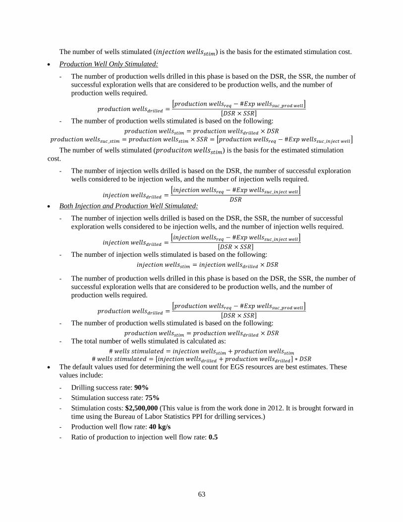
63

The number of wells stimulated (𝑃𝑃𝑃𝑃𝑝𝑝𝑃𝑃𝑃𝑃𝑃𝑃𝑃𝑃𝑃𝑃𝑃𝑃 𝑃𝑃𝑃𝑃𝑆𝑆𝑆𝑆𝑆𝑆𝑑𝑑𝑛𝑛𝑓𝑓𝑝𝑝) is the basis for the estimated stimulation cost.

• Production Well Only Stimulated:

- The number of production wells drilled in this phase is based on the DSR, the SSR, the number of successful exploration wells that are considered to be production wells, and the number of production wells required.

𝑃𝑃𝑃𝑃𝑃𝑃𝑑𝑑𝑃𝑃𝑃𝑃𝑃𝑃𝑃𝑃𝑃𝑃𝑃𝑃 𝑃𝑃𝑃𝑃𝑆𝑆𝑆𝑆𝑆𝑆𝑓𝑓𝑝𝑝𝑓𝑓𝑓𝑓𝑓𝑓𝑛𝑛𝑓𝑓 =�𝑃𝑃𝑃𝑃𝑃𝑃𝑑𝑑𝑃𝑃𝑃𝑃𝑃𝑃𝑃𝑃𝑃𝑃𝑃𝑃 𝑃𝑃𝑃𝑃𝑆𝑆𝑆𝑆𝑆𝑆𝑝𝑝𝑛𝑛𝑟𝑟 − #𝐿𝐿𝐼𝐼𝑃𝑃 𝑃𝑃𝑃𝑃𝑆𝑆𝑆𝑆𝑆𝑆𝑑𝑑𝑓𝑓𝑎𝑎_𝑝𝑝𝑝𝑝𝑔𝑔𝑓𝑓 𝑤𝑤𝑛𝑛𝑓𝑓𝑓𝑓�

[𝐷𝐷𝑆𝑆𝑅𝑅 × 𝑆𝑆𝑆𝑆𝑅𝑅]

- The number of production wells stimulated is based on the following: 𝑃𝑃𝑃𝑃𝑃𝑃𝑑𝑑𝑃𝑃𝑃𝑃𝑃𝑃𝑃𝑃𝑃𝑃𝑃𝑃 𝑃𝑃𝑃𝑃𝑆𝑆𝑆𝑆𝑆𝑆𝑑𝑑𝑛𝑛𝑓𝑓𝑝𝑝 = 𝑃𝑃𝑃𝑃𝑃𝑃𝑑𝑑𝑃𝑃𝑃𝑃𝑃𝑃𝑃𝑃𝑃𝑃𝑃𝑃 𝑃𝑃𝑃𝑃𝑆𝑆𝑆𝑆𝑆𝑆𝑓𝑓𝑝𝑝𝑓𝑓𝑓𝑓𝑓𝑓𝑛𝑛𝑓𝑓 × 𝐷𝐷𝑆𝑆𝑅𝑅

𝑃𝑃𝑃𝑃𝑃𝑃𝑑𝑑𝑃𝑃𝑃𝑃𝑃𝑃𝑃𝑃𝑃𝑃𝑃𝑃 𝑃𝑃𝑃𝑃𝑆𝑆𝑆𝑆𝑆𝑆𝑑𝑑𝑓𝑓𝑎𝑎_𝑑𝑑𝑛𝑛𝑓𝑓𝑝𝑝 = 𝑃𝑃𝑃𝑃𝑃𝑃𝑑𝑑𝑃𝑃𝑃𝑃𝑃𝑃𝑃𝑃𝑃𝑃𝑃𝑃 𝑃𝑃𝑃𝑃𝑆𝑆𝑆𝑆𝑆𝑆𝑑𝑑𝑛𝑛𝑓𝑓𝑝𝑝 × 𝑆𝑆𝑆𝑆𝑅𝑅 = �𝑃𝑃𝑃𝑃𝑃𝑃𝑑𝑑𝑃𝑃𝑃𝑃𝑃𝑃𝑃𝑃𝑃𝑃𝑃𝑃 𝑃𝑃𝑃𝑃𝑆𝑆𝑆𝑆𝑆𝑆𝑝𝑝𝑛𝑛𝑟𝑟 − #𝐿𝐿𝐼𝐼𝑃𝑃 𝑃𝑃𝑃𝑃𝑆𝑆𝑆𝑆𝑆𝑆𝑑𝑑𝑓𝑓𝑎𝑎_𝑓𝑓𝑛𝑛𝑝𝑝𝑛𝑛𝑎𝑎𝑛𝑛 𝑤𝑤𝑛𝑛𝑓𝑓𝑓𝑓�

The number of wells stimulated (𝑃𝑃𝑃𝑃𝑃𝑃𝑑𝑑𝑃𝑃𝑃𝑃𝑃𝑃𝑃𝑃𝑃𝑃𝑃𝑃 𝑃𝑃𝑃𝑃𝑆𝑆𝑆𝑆𝑆𝑆𝑑𝑑𝑛𝑛𝑓𝑓𝑝𝑝) is the basis for the estimated stimulation cost.

- The number of injection wells drilled is based on the DSR, the number of successful exploration wells considered to be injection wells, and the number of injection wells required.

𝑃𝑃𝑃𝑃𝑝𝑝𝑃𝑃𝑃𝑃𝑃𝑃𝑃𝑃𝑃𝑃𝑃𝑃 𝑃𝑃𝑃𝑃𝑆𝑆𝑆𝑆𝑆𝑆𝑓𝑓𝑝𝑝𝑓𝑓𝑓𝑓𝑓𝑓𝑛𝑛𝑓𝑓 =�𝑃𝑃𝑃𝑃𝑝𝑝𝑃𝑃𝑃𝑃𝑃𝑃𝑃𝑃𝑃𝑃𝑃𝑃 𝑃𝑃𝑃𝑃𝑆𝑆𝑆𝑆𝑆𝑆𝑝𝑝𝑛𝑛𝑟𝑟 − #𝐿𝐿𝐼𝐼𝑃𝑃 𝑃𝑃𝑃𝑃𝑆𝑆𝑆𝑆𝑆𝑆𝑑𝑑𝑓𝑓𝑎𝑎_𝑓𝑓𝑛𝑛𝑝𝑝𝑛𝑛𝑎𝑎𝑛𝑛 𝑤𝑤𝑛𝑛𝑓𝑓𝑓𝑓�

𝐷𝐷𝑆𝑆𝑅𝑅

• Both Injection and Production Well Stimulated:

- The number of injection wells drilled is based on the DSR, the SSR, the number of successful exploration wells considered to be injection wells, and the number of injection wells required.

𝑃𝑃𝑃𝑃𝑝𝑝𝑃𝑃𝑃𝑃𝑃𝑃𝑃𝑃𝑃𝑃𝑃𝑃 𝑃𝑃𝑃𝑃𝑆𝑆𝑆𝑆𝑆𝑆𝑓𝑓𝑝𝑝𝑓𝑓𝑓𝑓𝑓𝑓𝑛𝑛𝑓𝑓 =�𝑃𝑃𝑃𝑃𝑝𝑝𝑃𝑃𝑃𝑃𝑃𝑃𝑃𝑃𝑃𝑃𝑃𝑃 𝑃𝑃𝑃𝑃𝑆𝑆𝑆𝑆𝑆𝑆𝑝𝑝𝑛𝑛𝑟𝑟 − #𝐿𝐿𝐼𝐼𝑃𝑃 𝑃𝑃𝑃𝑃𝑆𝑆𝑆𝑆𝑆𝑆𝑑𝑑𝑓𝑓𝑎𝑎_𝑓𝑓𝑛𝑛𝑝𝑝𝑛𝑛𝑎𝑎𝑛𝑛 𝑤𝑤𝑛𝑛𝑓𝑓𝑓𝑓�

[𝐷𝐷𝑆𝑆𝑅𝑅 × 𝑆𝑆𝑆𝑆𝑅𝑅]

- The number of injection wells stimulated is based on the following: 𝑃𝑃𝑃𝑃𝑝𝑝𝑃𝑃𝑃𝑃𝑃𝑃𝑃𝑃𝑃𝑃𝑃𝑃 𝑃𝑃𝑃𝑃𝑆𝑆𝑆𝑆𝑆𝑆𝑑𝑑𝑛𝑛𝑓𝑓𝑝𝑝 = 𝑃𝑃𝑃𝑃𝑝𝑝𝑃𝑃𝑃𝑃𝑃𝑃𝑃𝑃𝑃𝑃𝑃𝑃 𝑃𝑃𝑃𝑃𝑆𝑆𝑆𝑆𝑆𝑆𝑓𝑓𝑝𝑝𝑓𝑓𝑓𝑓𝑓𝑓𝑛𝑛𝑓𝑓 × 𝐷𝐷𝑆𝑆𝑅𝑅

- The number of production wells drilled in this phase is based on the DSR, the SSR, the number of successful exploration wells that are considered to be production wells, and the number of production wells required.

𝑃𝑃𝑃𝑃𝑃𝑃𝑑𝑑𝑃𝑃𝑃𝑃𝑃𝑃𝑃𝑃𝑃𝑃𝑃𝑃 𝑃𝑃𝑃𝑃𝑆𝑆𝑆𝑆𝑆𝑆𝑓𝑓𝑝𝑝𝑓𝑓𝑓𝑓𝑓𝑓𝑛𝑛𝑓𝑓 =�𝑃𝑃𝑃𝑃𝑃𝑃𝑑𝑑𝑃𝑃𝑃𝑃𝑃𝑃𝑃𝑃𝑃𝑃𝑃𝑃 𝑃𝑃𝑃𝑃𝑆𝑆𝑆𝑆𝑆𝑆𝑝𝑝𝑛𝑛𝑟𝑟 − #𝐿𝐿𝐼𝐼𝑃𝑃 𝑃𝑃𝑃𝑃𝑆𝑆𝑆𝑆𝑆𝑆𝑑𝑑𝑓𝑓𝑎𝑎_𝑝𝑝𝑝𝑝𝑔𝑔𝑓𝑓 𝑤𝑤𝑛𝑛𝑓𝑓𝑓𝑓�

[𝐷𝐷𝑆𝑆𝑅𝑅 × 𝑆𝑆𝑆𝑆𝑅𝑅]

- The number of production wells stimulated is based on the following: 𝑃𝑃𝑃𝑃𝑃𝑃𝑑𝑑𝑃𝑃𝑃𝑃𝑃𝑃𝑃𝑃𝑃𝑃𝑃𝑃 𝑃𝑃𝑃𝑃𝑆𝑆𝑆𝑆𝑆𝑆𝑑𝑑𝑛𝑛𝑓𝑓𝑝𝑝 = 𝑃𝑃𝑃𝑃𝑃𝑃𝑑𝑑𝑃𝑃𝑃𝑃𝑃𝑃𝑃𝑃𝑃𝑃𝑃𝑃 𝑃𝑃𝑃𝑃𝑆𝑆𝑆𝑆𝑆𝑆𝑓𝑓𝑝𝑝𝑓𝑓𝑓𝑓𝑓𝑓𝑛𝑛𝑓𝑓 × 𝐷𝐷𝑆𝑆𝑅𝑅

- The total number of wells stimulated is calculated as: # 𝑃𝑃𝑃𝑃𝑆𝑆𝑆𝑆𝑆𝑆 𝑆𝑆𝑃𝑃𝑃𝑃𝑃𝑃𝑃𝑃𝑆𝑆𝑆𝑆𝑃𝑃𝑃𝑃𝑑𝑑 = 𝑃𝑃𝑃𝑃𝑝𝑝𝑃𝑃𝑃𝑃𝑃𝑃𝑃𝑃𝑃𝑃𝑃𝑃 𝑃𝑃𝑃𝑃𝑆𝑆𝑆𝑆𝑆𝑆𝑑𝑑𝑛𝑛𝑓𝑓𝑝𝑝 + 𝑃𝑃𝑃𝑃𝑃𝑃𝑑𝑑𝑃𝑃𝑃𝑃𝑃𝑃𝑃𝑃𝑃𝑃𝑃𝑃 𝑃𝑃𝑃𝑃𝑆𝑆𝑆𝑆𝑆𝑆𝑑𝑑𝑛𝑛𝑓𝑓𝑝𝑝

# 𝑃𝑃𝑃𝑃𝑆𝑆𝑆𝑆𝑆𝑆 𝑆𝑆𝑃𝑃𝑃𝑃𝑃𝑃𝑃𝑃𝑆𝑆𝑆𝑆𝑃𝑃𝑃𝑃𝑑𝑑 = [𝑃𝑃𝑃𝑃𝑝𝑝𝑃𝑃𝑃𝑃𝑃𝑃𝑃𝑃𝑃𝑃𝑃𝑃 𝑃𝑃𝑃𝑃𝑆𝑆𝑆𝑆𝑆𝑆𝑓𝑓𝑝𝑝𝑓𝑓𝑓𝑓𝑓𝑓𝑛𝑛𝑓𝑓 + 𝑃𝑃𝑃𝑃𝑃𝑃𝑑𝑑𝑃𝑃𝑃𝑃𝑃𝑃𝑃𝑃𝑃𝑃𝑃𝑃 𝑃𝑃𝑃𝑃𝑆𝑆𝑆𝑆𝑆𝑆𝑓𝑓𝑝𝑝𝑓𝑓𝑓𝑓𝑓𝑓𝑛𝑛𝑓𝑓] ∗ 𝐷𝐷𝑆𝑆𝑅𝑅 • The default values used for determining the well count for EGS resources are best estimates. These

values include:

- Drilling success rate: 90% - Stimulation success rate: 75% - Stimulation costs: $2,500,000 (This value is from the work done in 2012. It is brought forward in

time using the Bureau of Labor Statistics PPI for drilling services.) - Production well flow rate: 40 kg/s - Ratio of production to injection well flow rate: 0.5

64

Drilling Before/After PPA The number of wells that must be drilled before the PPA is obtained is determined based on the

number of wells required and the specified well field capacity that needs to be demonstrated in order to obtain the PPA. The well field capacity is the fraction of the required injection and production wells needed for the facility to operate. For example, if 60% of the well field capacity is required to obtain a PPA, and 10 successful production and five successful injection wells will be needed to operate at full capacity, then six successful production wells and three successful injection wells must be developed prior to obtaining the PPA. This would include any stimulation needed for a well to be considered successful.

Determining how many wells are drilled and stimulated prior to obtaining the PPA uses the same approach as is used in determining how many are drilled and stimulated for the entire project. The number of wells drilled and stimulated during the exploration phase remains the same. The number required for the Drilling phase is changed from that needed to support the project to that needed to get the PPA. Once the number drilled and stimulated are determined, the drilling and stimulation after the PPA is the difference between the values determined for the entire project and those required to obtain the PPA.

65

A6: DRILLING While the power plant may represent a larger monetary investment in the development of a

geothermal project, the uncertainty in drilling successful wells can put an entire project at risk. To acknowledge the potential for drilling failure, GETEM utilizes a drilling success rate to establish how many of the wells drilled will support the operation of the power plant, and includes the costs of unsuccessful wells when determining the power generation cost. If the down-select process is utilized (it is not the GETEM default) for the project evaluation, the generation cost will be included on all drilling costs, including those at sites drilled but not developed.

Exploration Drilling: Full-Size Wells The GETEM default during the Exploration phase is that every other full-size well drilled is

successful, or a 50% success rate. This drilling activity is effectively the confirmation phase in prior versions of GETEM. The prior default used for confirmation drilling success rate was 60% at the developed site, suggesting that the current default may be conservative. Figure 17 from Sanyal’s (2012) paper indicates there is considerable variation in this success rate. This figure provides drilling success curves for 12 well fields where 24 or more wells were drilled.

GETEM’s current default is that there are four to six full- size wells drilled during the exploration phase. Interpreting the success rate from Figure 17 in Sanyal’s (2012) paper is difficult for this number of wells because of the overlap of curves. An initial assessment of this data indicated a median after drilling both four and six wells to be ~50%, with the average being higher (~55% after four wells, and ~60% after six wells).

This paper indicates there is a learning curve in terms of the drilling rate (m/hr) as more wells are drilled. In the example given, the drilling rate increased from ~46 to 90% from the exploration phase to later in the field development (see Figure 19 of Sanyal’s [2012] paper), or, conversely, the rates given indicate they were 32 to 47% lower during the early drilling activities. Well costs were estimated using these lower drilling rates, or rates of penetration (ROP), using the SNL cost models. The well costs during exploration were higher as indicted in Figure A-6 below.

Figure A-6. The effect of lower drilling rates on well cost based on the SNL models.

66

The GETEM default for the effect of this learning curve on well costs is 1.2, which represents the impact of the 32% lower ROP. Using this data to establish a relative cost is speculative because total well counts determined for the scenarios considered in GETEM are generally lower than those in Sanyal’s (2012) paper; however, this work does indicate that there is a learning curve and that as more wells are drilled, the drilling rate (m/hr) increases. Wells initially drilled should be expected to cost more, and though the amount of data is limited, the GETEM default of 20% higher is not improbable.

Drilling Phase Success Rate

Sanyal’s (2012) paper indicates that in the survey of drilling success rates, the average value of a project was ~68%. As apparent in Figure 17 of Sanyal’s paper, there is considerable variation in this success rate (33 to 100%), with the prevalent range between 60 and 80%.

There are questions that arise when reviewing this paper and integrating the information presented into GETEM:

• The criteria for success is a minimum of 3 MW capacity, which implies this is the success for a production well. The success criteria for injection wells is not specified, and as such, it is not known if injection wells are included in the assessment.

• Presumably there is drilling of makeup wells included in the data presented. It is not clear if the wells are considered successful if they are taken out of service and replaced with a makeup well.

• Most of the well fields that are included in the survey have more wells drilled than would typically be drilled in a scenario evaluated by GTO.

• It is unclear whether some of these projects received any government support. Unless the wells are inexpensive to drill and/or extremely productive, it would be difficult for a geothermal project in the U.S. to be economically competitive with success rates of 50% or less for the entire well field.

Though there are questions, the information in the paper provides a basis for establishing default inputs for GETEM. To do so, the following assumptions are made:

• The drilling success rates presented are for both production and injection wells.

• Wells that are used to support plant operation are successful even if they are eventually replaced with makeup wells.

• The differences in project size are ignored, as is the potential that some may have received government support.

One difference between GETEM’s depiction of drilling success and that described in Sanyal’s (2012) paper is that GETEM uses two drilling success rates—one for the early project activities and one for the final drilling phase to complete the well field. The average value reported by Sanyal is based on all drilling activities. Figure A-7 below illustrates GETEM’s effective success rate for the entire project that is analogous to the average for the well field. On the left is the effective rate with the current GETEM default of 50% during exploration; on the right is for a 60% success rate during exploration. The blue shaded box is the range of likely values from Sanyal’s paper. The number of wells required is typical of the scenarios being evaluated in GETEM by GTO.

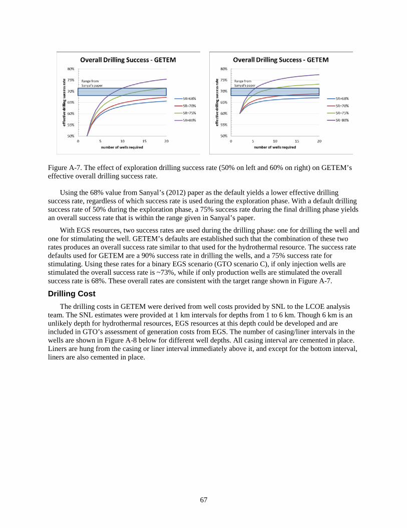
67

Figure A-7. The effect of exploration drilling success rate (50% on left and 60% on right) on GETEM’s effective overall drilling success rate.

Using the 68% value from Sanyal’s (2012) paper as the default yields a lower effective drilling success rate, regardless of which success rate is used during the exploration phase. With a default drilling success rate of 50% during the exploration phase, a 75% success rate during the final drilling phase yields an overall success rate that is within the range given in Sanyal’s paper.

With EGS resources, two success rates are used during the drilling phase: one for drilling the well and one for stimulating the well. GETEM’s defaults are established such that the combination of these two rates produces an overall success rate similar to that used for the hydrothermal resource. The success rate defaults used for GETEM are a 90% success rate in drilling the wells, and a 75% success rate for stimulating. Using these rates for a binary EGS scenario (GTO scenario C), if only injection wells are stimulated the overall success rate is ~73%, while if only production wells are stimulated the overall success rate is 68%. These overall rates are consistent with the target range shown in Figure A-7.

Drilling Cost The drilling costs in GETEM were derived from well costs provided by SNL to the LCOE analysis

team. The SNL estimates were provided at 1 km intervals for depths from 1 to 6 km. Though 6 km is an unlikely depth for hydrothermal resources, EGS resources at this depth could be developed and are included in GTO’s assessment of generation costs from EGS. The number of casing/liner intervals in the wells are shown in Figure A-8 below for different well depths. All casing interval are cemented in place. Liners are hung from the casing or liner interval immediately above it, and except for the bottom interval, liners are also cemented in place.

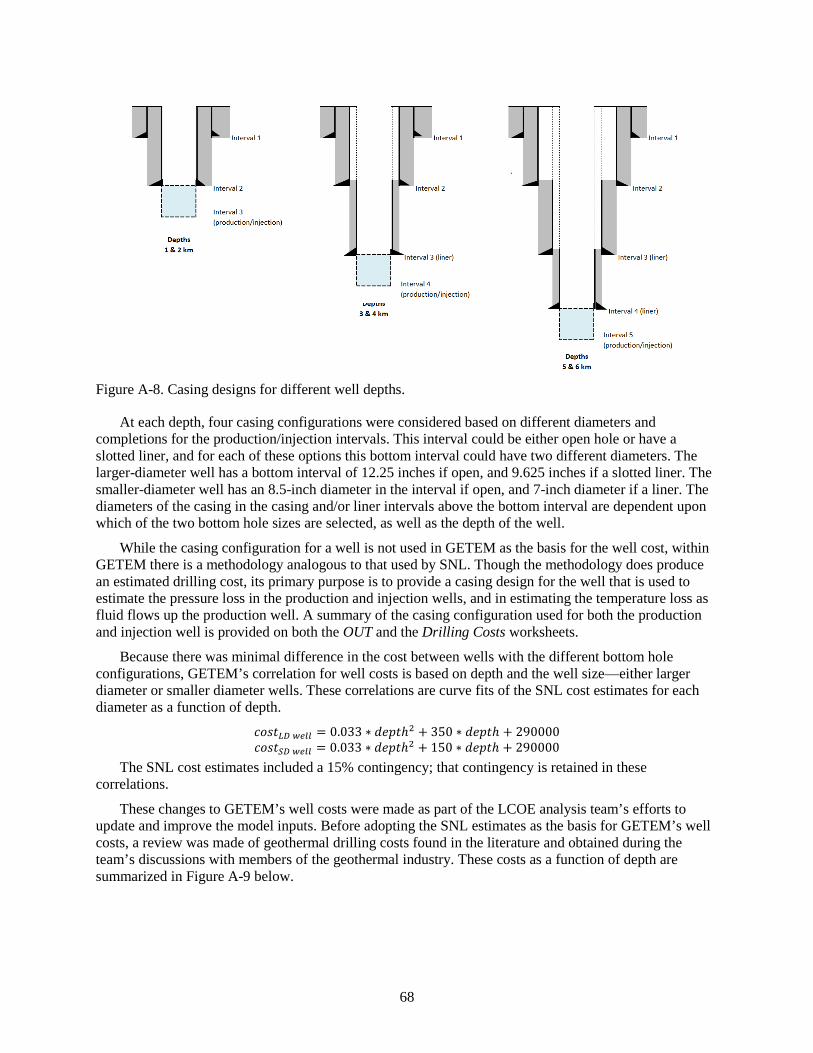
68

Figure A-8. Casing designs for different well depths.

At each depth, four casing configurations were considered based on different diameters and completions for the production/injection intervals. This interval could be either open hole or have a slotted liner, and for each of these options this bottom interval could have two different diameters. The larger-diameter well has a bottom interval of 12.25 inches if open, and 9.625 inches if a slotted liner. The smaller-diameter well has an 8.5-inch diameter in the interval if open, and 7-inch diameter if a liner. The diameters of the casing in the casing and/or liner intervals above the bottom interval are dependent upon which of the two bottom hole sizes are selected, as well as the depth of the well.

While the casing configuration for a well is not used in GETEM as the basis for the well cost, within GETEM there is a methodology analogous to that used by SNL. Though the methodology does produce an estimated drilling cost, its primary purpose is to provide a casing design for the well that is used to estimate the pressure loss in the production and injection wells, and in estimating the temperature loss as fluid flows up the production well. A summary of the casing configuration used for both the production and injection well is provided on both the OUT and the Drilling Costs worksheets.

Because there was minimal difference in the cost between wells with the different bottom hole configurations, GETEM’s correlation for well costs is based on depth and the well size—either larger diameter or smaller diameter wells. These correlations are curve fits of the SNL cost estimates for each diameter as a function of depth.

𝑃𝑃𝑃𝑃𝑆𝑆𝑃𝑃𝐿𝐿𝐷𝐷 𝑤𝑤𝑛𝑛𝑓𝑓𝑓𝑓 = 0.033 ∗ 𝑑𝑑𝑃𝑃𝑃𝑃𝑃𝑃ℎ2 + 350 ∗ 𝑑𝑑𝑃𝑃𝑃𝑃𝑃𝑃ℎ + 290000 𝑃𝑃𝑃𝑃𝑆𝑆𝑃𝑃𝑆𝑆𝐷𝐷 𝑤𝑤𝑛𝑛𝑓𝑓𝑓𝑓 = 0.033 ∗ 𝑑𝑑𝑃𝑃𝑃𝑃𝑃𝑃ℎ2 + 150 ∗ 𝑑𝑑𝑃𝑃𝑃𝑃𝑃𝑃ℎ + 290000

The SNL cost estimates included a 15% contingency; that contingency is retained in these correlations.

These changes to GETEM’s well costs were made as part of the LCOE analysis team’s efforts to update and improve the model inputs. Before adopting the SNL estimates as the basis for GETEM’s well costs, a review was made of geothermal drilling costs found in the literature and obtained during the team’s discussions with members of the geothermal industry. These costs as a function of depth are summarized in Figure A-9 below.

69

Figure A-9. Summary of drilling costs collected from literature and geothermal industry interviews.

For the costs from the different sources to be comparable to the GETEM correlations it was necessary to bring those costs to an equivalent point in time. That point was 2010, which is the basis of the costs provided by SNL and the basis for the GETEM correlations. This was accomplished using the PPI for drilling oil and gas wells, obtained from the U.S. Bureau of Labor Statistics. With this adjustment to the costs from the different sources, the cost correlations based on the SNL estimates (also shown in this figure) were deemed representative of geothermal drilling costs and the correlations incorporated into GETEM.

Since GETEM was originally developed in 2004–2006, there has been considerable variation in drilling costs. That volatility is captured in GETEM using the PPI for oil and gas well drilling. When a year is selected for analysis, this PPI is applied to the year 2010 costs determined using one of the two cost correlations. With the PPI applied, the drilling cost is representative of costs in the year for which the analysis is being made. Figure A-10 shows how the PPI used has varied with time. It illustrates how drilling costs have varied over relatively short periods of time, and serves to emphasize the importance of updating GETEM’s PPIs before estimating current costs.

70

Figure A-10. Time variation of the producer price index for drilling oil and gas wells.

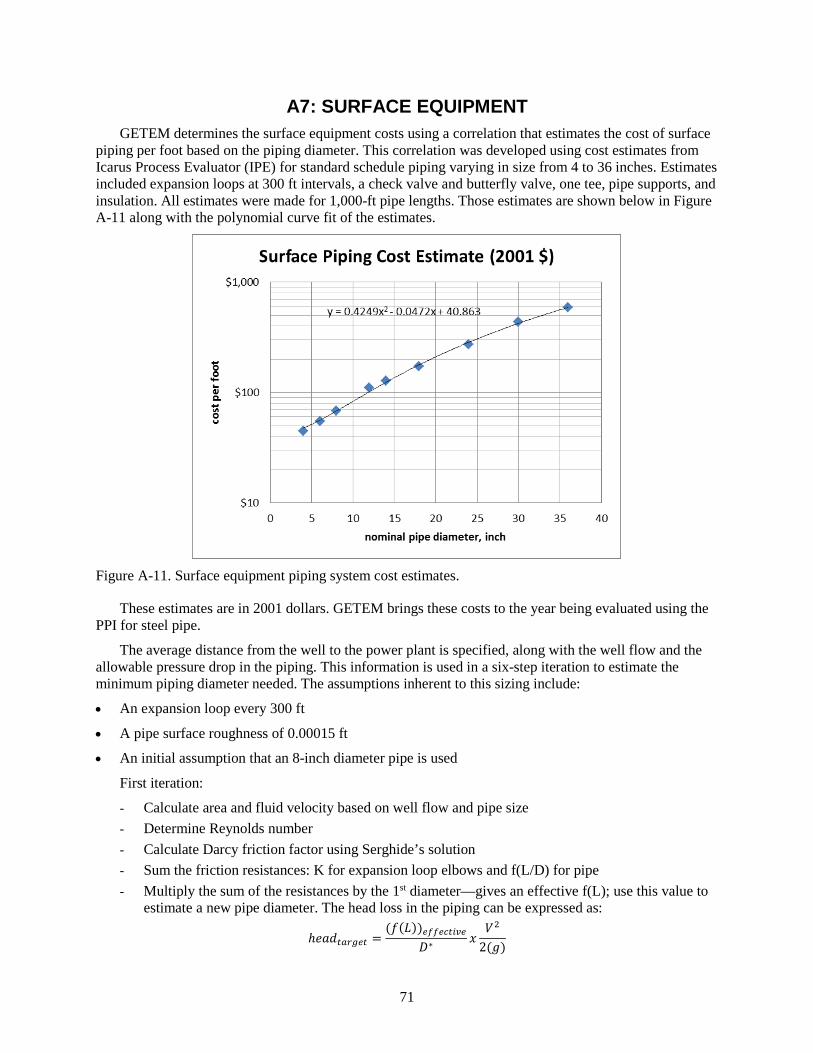
71

A7: SURFACE EQUIPMENT GETEM determines the surface equipment costs using a correlation that estimates the cost of surface

piping per foot based on the piping diameter. This correlation was developed using cost estimates from Icarus Process Evaluator (IPE) for standard schedule piping varying in size from 4 to 36 inches. Estimates included expansion loops at 300 ft intervals, a check valve and butterfly valve, one tee, pipe supports, and insulation. All estimates were made for 1,000-ft pipe lengths. Those estimates are shown below in Figure A-11 along with the polynomial curve fit of the estimates.

Figure A-11. Surface equipment piping system cost estimates.

These estimates are in 2001 dollars. GETEM brings these costs to the year being evaluated using the PPI for steel pipe.

The average distance from the well to the power plant is specified, along with the well flow and the allowable pressure drop in the piping. This information is used in a six-step iteration to estimate the minimum piping diameter needed. The assumptions inherent to this sizing include:

• An expansion loop every 300 ft

• A pipe surface roughness of 0.00015 ft

• An initial assumption that an 8-inch diameter pipe is used

First iteration:

- Calculate area and fluid velocity based on well flow and pipe size - Determine Reynolds number - Calculate Darcy friction factor using Serghide’s solution - Sum the friction resistances: K for expansion loop elbows and f(L/D) for pipe - Multiply the sum of the resistances by the 1st diameter—gives an effective f(L); use this value to

estimate a new pipe diameter. The head loss in the piping can be expressed as:

ℎ𝑃𝑃𝑆𝑆𝑑𝑑𝑛𝑛𝑝𝑝𝑝𝑝𝑔𝑔𝑛𝑛𝑛𝑛 =(𝑓𝑓(𝐿𝐿))𝑛𝑛𝑓𝑓𝑓𝑓𝑛𝑛𝑎𝑎𝑛𝑛𝑓𝑓𝑎𝑎𝑛𝑛

𝐷𝐷∗ 𝐼𝐼𝑃𝑃2

2(𝑃𝑃)

72

In this expression headtarget is head loss corresponding to the allowable ΔP. Velocity (V) and f(L)effective are determined using the initial diameter. This relationship is used to solve for the diameter (D*) that would be needed with this velocity and frictional losses to produce the targeted head loss.

𝐷𝐷∗ =(𝑓𝑓(𝐿𝐿))𝑛𝑛𝑓𝑓𝑓𝑓𝑛𝑛𝑎𝑎𝑛𝑛𝑓𝑓𝑎𝑎𝑛𝑛ℎ𝑃𝑃𝑆𝑆𝑑𝑑𝑛𝑛𝑝𝑝𝑝𝑝𝑔𝑔𝑛𝑛𝑛𝑛

𝐼𝐼𝑃𝑃2

2(𝑃𝑃)

This diameter is used to estimate the next diameter used in the iteration process. In the above relationship V∝ D2; the diameter that would give the velocity and frictional losses that would result in the targeted head loss is

𝐷𝐷2 = 𝐷𝐷1 × �𝐷𝐷∗

𝐷𝐷1�0.25

This new diameter is used to repeat the above calculations to determine the velocity, friction losses, the diameter needed to produce the targeted head loss, and the new diameter. After the initial estimate of 8 inches, this iteration is repeated five more times. At that point, the estimated diameter converging on the minimum diameter that would satisfy the maximum pressure drop criteria is given.

This diameter is used in the correlation

𝑆𝑆𝑃𝑃𝑃𝑃𝑓𝑓𝑆𝑆𝑃𝑃𝑃𝑃 𝑃𝑃𝑒𝑒𝑃𝑃𝑃𝑃𝑃𝑃𝑃𝑃𝑃𝑃𝑃𝑃𝑃𝑃 𝑃𝑃𝑃𝑃𝑆𝑆𝑃𝑃𝑝𝑝𝑛𝑛𝑝𝑝 𝑓𝑓𝑔𝑔𝑔𝑔𝑛𝑛 = 0.4249 × 𝐷𝐷𝑓𝑓2 − 0.0472 × 𝐷𝐷𝑓𝑓 + 40.863

This cost is in 2001 dollars. The PPI for pipe is applied to bring the estimate to current dollars (or the year being evaluated). The updated cost is multiplied by the specified distance between the well and plant to determine the surface equipment cost per well. This cost is applied to all wells supporting plant operations.

This approach is used for both binary and flash plants, recognizing that the approach used to size the piping is based upon the properties of liquid water. With flash plants, it is probable that the geothermal flow in the production surface piping will be two-phase, and the approach described will underestimate the size and cost of the piping required. This is, in part, why GETEM’s default for the allowable pressure drop is lower (5 psid) for flash plants.

The surface equipment costs that are estimated do not include any separators or other equipment at individual wellheads. Nor does GETEM attempt to define surface piping systems where fluid from individual wells would flow to or from a main production or injection line going to or from a plant.

73

A8: GEOTHERMAL PUMPING Pumps are utilized with geothermal resources to increase flow, and by doing so reduce the number of

wells required to support a specified level of power sales, or increase the power sales from a fixed number of wells. There are costs associated with this pumping that diminish, and in some instances negate, the benefits of increasing flow. These costs include the capital and maintenance costs for the pumps, as well as power needed to operate the pumps.

In GETEM, the power needed for operating the geothermal pumps is assumed to be generated by the power plant. The power sales for a project is the difference between the net output from the power plant and this geothermal pumping. Figure A-12 below illustrates the impact of pumping on power sales. It plots the fraction of the plant output required for production well pumping as a function of the required pump setting depth for three different temperatures.

Figure A-12. The impact of production pumping on power sales.

This figure is idealized in that it assumes that the flow rate is constant at all pump depths, that friction losses are negligible, and that the pump suction pressure is equivalent to the fluid pressure at the production wellhead. With these assumptions, the head developed by the pump is equivalent to the setting depth, and the results shown do not change regardless of the magnitude of the flow rate assumed. The sensitivity of power to resource temperature results from lower temperature fluids having less potential to produce work; the specific pumping power (power per unit mass flow) is the same for all temperatures at a given depth.

Geothermal pumping also includes the injection pumping power. With the assumptions made, results for injection pumping are the same when the required injection pump head and the pump production depth are equivalent and the produced and injected flow are the same. For example, a well with a temperature of 150°C and a production pump depth of 400 m, ~15% of the plant output would be required for the production pump. If the required injection pump head were 400 m, then ~15% of the plant output would also be required for the injection pump, or a total of ~30% of the plant output needed for geothermal pumping.

74

Though this is an idealized representation of pumping power, it is informative in that it illustrates that there is a cost associated with pumping that increases with flow rate per well. Because of this cost, there is an economic optimum where the effect of the added pumping power to increase well flow offsets the reduction in well count associated with that increased flow per well.

In GETEM’s determination of pumping power, both the pumping depth required and the injection pump head are determined. These determinations are functions of the input provided and calculations made; they include the effects of friction, any difference in the flow to an injection well and a production well, fluid temperature losses in the well bore, hydrostatic pressure, well depth, and the well casing design.

Approach The conversion system used establishes whether a production well will default to having a downhole

production pump. Binary plants default to having production pumps; flash steam plants default to having artesian flow production wells. One can revise these defaults, and GETEM will calculate an LCOE even though it is probable that with binary plants, warnings will be received that flashing has occurred in the production well. Note that if flashing occurs, GETEM does not revise its estimate of the production wellhead temperature used for binary plants (the assumption remains that geothermal fluid at the wellhead is a single phase liquid).

Figure A-13 below shows key parameters that the model uses in determining the setting depth for the production pump and the injection pump head.

Figure A-13. Key parameters used in determining the setting depth for the production pump and the injection pump head.

The following sections provide specifics as to how GETEM determines these parameters when they are not specified inputs.

75

Hydrostatic Pressure GETEM’s calculation of pumping power is based on its estimate of the pressure in the reservoir. This

reservoir pressure essentially “pushes” fluid up the production well, and “pushes” against any fluid being injected. In determining pumping power, this reservoir pressure is represented by hydrostatic pressure, or the pressure of a column of water having height equivalent to the resource depth, with the water column being in thermal equilibrium with the earth from the surface to the bottom of the production well. Xie, Bloomfield, and Shook (2005) used the following correlation for the hydrostatic pressure:

𝑃𝑃𝑝𝑝(ℎ) = 𝑃𝑃𝑔𝑔 +1𝐿𝐿𝑝𝑝�𝑃𝑃𝜌𝜌𝑜𝑜𝑔𝑔𝐿𝐿𝑝𝑝�ℎ−

𝐿𝐿𝑇𝑇2 Г𝑇𝑇ℎ

2� − 1�

Po, ρo = fluid pressure and density at surface condition

CP = pressure gradient

CT = temperature gradient coefficient

h = reservoir depth

ГT = earth temperature gradient.

For a typical hydrothermal reservoir, the authors used CP = 4.64 × 10-7 KPa−1 or 4.64 × 105 bar−1 and CT = 9 × 10-4°C−1.

The temperature gradient coefficient was modified for use in GETEM as shown below. This modification was made after comparing the pressure calculated with the above correlation to the density head of water calculated at 5-meter intervals from the surface to depth. At each interval, the fluid temperature increased according to an earth temperature gradient, which was used to determine the density of the fluid using the pressure of the immediate above interval. This density head calculation indicated that for the deepest wells being considered for EGS, the above correlation predicted pressures that were ~4% lower, indicated by the density head calculation. The effect of a lower hydrostatic pressure is to increase the pump setting depth and the production pumping power that is required. With the correction to the temperature gradient coefficient given below, the correlation produces hydrostatic pressures that are ~0.5% lower than the calculated density head for depths to 6 km.

𝐿𝐿𝑇𝑇,𝑝𝑝𝑛𝑛𝑎𝑎𝑓𝑓𝑑𝑑𝑛𝑛𝑓𝑓 = 9× 10−4

�30.796×𝑇𝑇𝑅𝑅−0.552�, °𝐿𝐿−1where TR is the resource temperature in °C

GETEM’s determination of both production and injection pumping power is dependent upon the bottom hole pressure in the well. For hydrothermal resources, the bottom hole pressures are:

𝑃𝑃𝑝𝑝𝑝𝑝𝑔𝑔𝑓𝑓𝑓𝑓𝑎𝑎𝑛𝑛𝑓𝑓𝑔𝑔𝑛𝑛−𝑏𝑏𝑔𝑔𝑛𝑛𝑛𝑛𝑔𝑔𝑝𝑝 ℎ𝑔𝑔𝑓𝑓𝑛𝑛 = 𝑃𝑃ℎ𝑎𝑎𝑓𝑓𝑝𝑝𝑔𝑔𝑑𝑑𝑛𝑛𝑝𝑝𝑛𝑛𝑓𝑓𝑎𝑎 − 𝑑𝑑𝑃𝑃𝑆𝑆𝑃𝑃𝑑𝑑𝑃𝑃𝑃𝑃𝑃𝑃𝑝𝑝𝑝𝑝𝑔𝑔𝑓𝑓𝑓𝑓𝑎𝑎𝑛𝑛𝑓𝑓𝑔𝑔𝑛𝑛 𝑤𝑤𝑛𝑛𝑓𝑓𝑓𝑓 𝑃𝑃𝑓𝑓𝑛𝑛𝑝𝑝𝑛𝑛𝑎𝑎𝑓𝑓𝑛𝑛𝑔𝑔𝑛𝑛−𝑏𝑏𝑔𝑔𝑛𝑛𝑛𝑛𝑔𝑔𝑝𝑝 ℎ𝑔𝑔𝑓𝑓𝑛𝑛 = 𝑃𝑃ℎ𝑎𝑎𝑓𝑓𝑝𝑝𝑔𝑔𝑑𝑑𝑛𝑛𝑝𝑝𝑛𝑛𝑓𝑓𝑎𝑎 + 𝑏𝑏𝑃𝑃𝑃𝑃𝑆𝑆𝑑𝑑𝑃𝑃𝑃𝑃𝑓𝑓𝑛𝑛𝑝𝑝𝑛𝑛𝑎𝑎𝑛𝑛𝑓𝑓𝑔𝑔𝑛𝑛 𝑤𝑤𝑛𝑛𝑓𝑓𝑓𝑓

In these relationships, the buildup at the injection well and the drawdown at the production well are hydraulic resistance terms that are functions of flow rate.

With EGS scenarios, there is a direct connection between the production and injection well in the reservoir created. With this resource, the bottom hole pressure in the production well can be expressed as:

𝑃𝑃𝑝𝑝𝑝𝑝𝑔𝑔𝑓𝑓𝑓𝑓𝑎𝑎𝑛𝑛𝑓𝑓𝑔𝑔𝑛𝑛−𝑏𝑏𝑔𝑔𝑛𝑛𝑛𝑛𝑔𝑔𝑝𝑝 ℎ𝑔𝑔𝑓𝑓𝑛𝑛 = 𝑃𝑃𝑓𝑓𝑛𝑛𝑝𝑝𝑛𝑛𝑎𝑎𝑛𝑛𝑓𝑓𝑔𝑔𝑛𝑛−𝑏𝑏𝑔𝑔𝑛𝑛𝑛𝑛𝑔𝑔𝑝𝑝 ℎ𝑔𝑔𝑓𝑓𝑛𝑛 − 𝐵𝐵𝑃𝑃𝑃𝑃𝑆𝑆𝑑𝑑𝑃𝑃𝑃𝑃𝑓𝑓𝑛𝑛𝑝𝑝𝑛𝑛𝑎𝑎𝑛𝑛𝑓𝑓𝑔𝑔𝑛𝑛 𝑤𝑤𝑛𝑛𝑓𝑓𝑓𝑓 − 𝐷𝐷𝑃𝑃𝑆𝑆𝑃𝑃𝑑𝑑𝑃𝑃𝑃𝑃𝑃𝑃𝑝𝑝𝑝𝑝𝑔𝑔𝑓𝑓𝑓𝑓𝑎𝑎𝑛𝑛𝑓𝑓𝑔𝑔𝑛𝑛 𝑤𝑤𝑛𝑛𝑓𝑓𝑓𝑓

The buildup and drawdown terms in this relationship again represent the hydraulic resistance to flow—in this case, in combination they represent this resistance for the reservoir created.

With EGS resources it is assumed that there will be a hydrostatic pressure that will have to be overcome in order to inject fluid.

𝑃𝑃𝑓𝑓𝑛𝑛𝑝𝑝𝑛𝑛𝑎𝑎𝑛𝑛𝑓𝑓𝑔𝑔𝑛𝑛−𝑏𝑏𝑔𝑔𝑛𝑛𝑛𝑛𝑔𝑔𝑝𝑝 ℎ𝑔𝑔𝑓𝑓𝑛𝑛 = 𝑃𝑃ℎ𝑎𝑎𝑓𝑓𝑝𝑝𝑔𝑔𝑑𝑑𝑛𝑛𝑝𝑝𝑛𝑛𝑓𝑓𝑎𝑎 + 𝑏𝑏𝑃𝑃𝑃𝑃𝑆𝑆𝑑𝑑𝑃𝑃𝑃𝑃𝑓𝑓𝑛𝑛𝑝𝑝𝑛𝑛𝑎𝑎𝑛𝑛𝑓𝑓𝑔𝑔𝑛𝑛 𝑤𝑤𝑛𝑛𝑓𝑓𝑓𝑓 𝑃𝑃𝑓𝑓𝑛𝑛𝑝𝑝𝑛𝑛𝑎𝑎𝑛𝑛𝑓𝑓𝑔𝑔𝑛𝑛−𝑏𝑏𝑔𝑔𝑛𝑛𝑛𝑛𝑔𝑔𝑝𝑝 ℎ𝑔𝑔𝑓𝑓𝑛𝑛 = 𝑃𝑃𝑝𝑝𝑓𝑓𝑝𝑝𝑛𝑛𝑛𝑛 𝑔𝑔𝑓𝑓𝑛𝑛𝑓𝑓𝑛𝑛𝑛𝑛 + 𝑑𝑑𝑃𝑃𝑃𝑃𝑆𝑆𝑃𝑃𝑃𝑃𝑐𝑐 ℎ𝑃𝑃𝑆𝑆𝑑𝑑, 𝑃𝑃𝑃𝑃 𝜌𝜌 ∗ 𝑑𝑑𝑃𝑃𝑃𝑃𝑃𝑃ℎ − ∆𝑃𝑃𝑓𝑓𝑝𝑝𝑓𝑓𝑎𝑎𝑛𝑛𝑓𝑓𝑔𝑔𝑛𝑛

76

The larger of these two values for the bottom hole pressure in the injection well is used in determining the bottom hole pressure in the EGS production well.

Production Well Pump Depth

For a given resource, increasing production flow from a well requires increasing the depth at which the pump is set. That setting depth corresponds to the location in the well where a minimum allowable pressure occurs; this is the minimum suction pressure for the production pump. In GETEM, this minimum pressure is

𝑃𝑃𝑝𝑝𝑓𝑓𝑛𝑛𝑓𝑓𝑝𝑝𝑓𝑓𝑝𝑝 = 𝑃𝑃𝑑𝑑𝑝𝑝𝑛𝑛𝑓𝑓𝑝𝑝𝑝𝑝𝑛𝑛𝑓𝑓𝑔𝑔𝑛𝑛 + 𝑃𝑃𝑛𝑛𝑎𝑎𝑔𝑔 + 𝑁𝑁𝑃𝑃𝑆𝑆𝑁𝑁

where

Psaturation is the saturation pressure at the fluid temperature

Pncg is the pressure necessary to keep non-condensable gases in solution

NPSH is the net positive suction head for the pump.

GETEM determines a saturation pressure; the other two terms are combined as a single input value to the model (the excess pressure at the pump suction, or Pexcess).

𝑃𝑃𝑛𝑛𝑒𝑒𝑎𝑎𝑛𝑛𝑑𝑑𝑑𝑑 = 𝑃𝑃𝑛𝑛𝑎𝑎𝑔𝑔 + 𝑁𝑁𝑃𝑃𝑆𝑆𝑁𝑁

This term represents the pressure needed above saturation to prevent pump cavitation. It assumed the minimum pressure (Pminimum) is also the pressure at the production wellhead, with the defined excess pressure keeping the fluid from flashing between the wellhead and the power plant (binary plant heat exchangers). The minimum pressure can also be expressed as:

𝑃𝑃𝑝𝑝𝑓𝑓𝑛𝑛𝑓𝑓𝑝𝑝𝑓𝑓𝑝𝑝 = 𝑃𝑃𝑏𝑏𝑔𝑔𝑛𝑛𝑛𝑛𝑔𝑔𝑝𝑝 ℎ𝑔𝑔𝑓𝑓𝑛𝑛 − ∆𝑃𝑃𝑓𝑓𝑝𝑝𝑓𝑓𝑎𝑎𝑓𝑓𝑛𝑛𝑔𝑔𝑛𝑛 − 𝜌𝜌𝑔𝑔𝑓𝑓(ℎ𝑏𝑏𝑔𝑔𝑛𝑛𝑛𝑛𝑔𝑔𝑝𝑝),

where

ΔPfriction is the friction loss as the fluid flows up the well

ρgf is the density of the geothermal fluid

hbottom is the distance from the bottom of the well to the location where the minimum pressure occurs.

The difference between the depth of the well (Dwell) and the point in the well where the minimum pressure occurs (hbottom) is the pump depth (dpump). This allows the minimum pressure to be expressed as:

𝑃𝑃𝑝𝑝𝑓𝑓𝑛𝑛𝑓𝑓𝑝𝑝𝑓𝑓𝑝𝑝 = 𝑃𝑃𝑏𝑏𝑔𝑔𝑛𝑛𝑛𝑛𝑔𝑔𝑝𝑝 ℎ𝑔𝑔𝑓𝑓𝑛𝑛 − ∆𝑃𝑃𝑓𝑓𝑝𝑝𝑓𝑓𝑎𝑎𝑓𝑓𝑛𝑛𝑔𝑔𝑛𝑛 − 𝜌𝜌𝑔𝑔𝑓𝑓(𝐷𝐷𝑤𝑤𝑛𝑛𝑓𝑓𝑓𝑓 − 𝑑𝑑𝑝𝑝𝑓𝑓𝑝𝑝𝑝𝑝)

The two expressions for the minimum pressure can be combined, producing the following solution for the pump depth, dpump.

𝑑𝑑𝑝𝑝𝑓𝑓𝑝𝑝𝑝𝑝 = 𝐷𝐷𝑤𝑤𝑛𝑛𝑓𝑓𝑓𝑓 − �𝑃𝑃𝑏𝑏𝑔𝑔𝑛𝑛𝑛𝑛𝑔𝑔𝑝𝑝 ℎ𝑔𝑔𝑓𝑓𝑛𝑛 − ∆𝑃𝑃𝑓𝑓𝑝𝑝𝑓𝑓𝑎𝑎𝑛𝑛𝑓𝑓𝑔𝑔𝑛𝑛 − 𝑃𝑃𝑑𝑑𝑝𝑝𝑛𝑛𝑓𝑓𝑝𝑝𝑝𝑝𝑛𝑛𝑓𝑓𝑔𝑔𝑛𝑛 − 𝑃𝑃𝑛𝑛𝑒𝑒𝑎𝑎𝑛𝑛𝑑𝑑𝑑𝑑

𝜌𝜌𝑔𝑔𝑓𝑓�

As indicated, the bottom hole pressure in the production well is the hydrostatic pressure less the drawdown. In GETEM, this bottom hole pressure is determined as:

𝑃𝑃𝑝𝑝𝑝𝑝𝑔𝑔𝑓𝑓𝑓𝑓𝑎𝑎𝑛𝑛𝑓𝑓𝑔𝑔𝑛𝑛−𝑏𝑏𝑔𝑔𝑛𝑛𝑛𝑛𝑔𝑔𝑝𝑝 ℎ𝑔𝑔𝑓𝑓𝑛𝑛 = 𝑃𝑃ℎ𝑎𝑎𝑓𝑓𝑝𝑝𝑔𝑔𝑑𝑑𝑛𝑛𝑝𝑝𝑛𝑛𝑓𝑓𝑎𝑎 − 𝑑𝑑𝑃𝑃𝑆𝑆𝑃𝑃𝑑𝑑𝑃𝑃𝑃𝑃𝑃𝑃, where

𝑑𝑑𝑃𝑃𝑆𝑆𝑃𝑃𝑑𝑑𝑃𝑃𝑃𝑃𝑃𝑃 = 𝑓𝑓𝑆𝑆𝑃𝑃𝑃𝑃 𝑃𝑃𝑆𝑆𝑃𝑃𝑃𝑃𝑤𝑤𝑛𝑛𝑓𝑓𝑓𝑓

𝑃𝑃𝑃𝑃𝑃𝑃𝑑𝑑𝑃𝑃𝑃𝑃𝑃𝑃𝑃𝑃𝑙𝑙𝑃𝑃𝑃𝑃𝑐𝑐 𝑃𝑃𝑃𝑃𝑑𝑑𝑃𝑃𝐼𝐼

Both the flow rate per well and the productivity index are specified inputs.

GETEM determines the pump setting depth by first solving for the pressure at the bottom of the upper casing interval, with the premise that the production pump will be set in this casing interval, which will

77

have a 13 5/8-inch diameter casing (or larger) in order to accommodate the production pump. This pressure is determined by calculating the pressure change in each interval below the upper casing in the well.

𝑃𝑃𝑏𝑏𝑔𝑔𝑛𝑛𝑛𝑛𝑔𝑔𝑝𝑝 𝑓𝑓𝑝𝑝𝑝𝑝𝑛𝑛𝑝𝑝 𝑎𝑎𝑝𝑝𝑑𝑑𝑓𝑓𝑛𝑛𝑔𝑔 𝑓𝑓𝑛𝑛𝑛𝑛𝑛𝑛𝑝𝑝𝑎𝑎𝑝𝑝𝑓𝑓 = 𝑃𝑃𝑏𝑏𝑔𝑔𝑛𝑛𝑛𝑛𝑔𝑔𝑝𝑝 ℎ𝑔𝑔𝑓𝑓𝑛𝑛 − � �∆𝑃𝑃𝑓𝑓𝑛𝑛𝑝𝑝𝑛𝑛ℎ + ∆𝑃𝑃𝑓𝑓𝑝𝑝𝑓𝑓𝑎𝑎𝑛𝑛𝑓𝑓𝑔𝑔𝑛𝑛�#𝑓𝑓𝑛𝑛𝑛𝑛𝑛𝑛𝑝𝑝𝑎𝑎𝑝𝑝𝑓𝑓𝑑𝑑−1

1

In this relationship, ΔPdepth is the change in the density head across an interval. ∆𝑃𝑃𝑓𝑓𝑛𝑛𝑝𝑝𝑛𝑛ℎ = 𝜌𝜌𝑔𝑔𝑓𝑓 ∗ ℎ𝑃𝑃𝑃𝑃𝑃𝑃ℎ𝑃𝑃𝑓𝑓𝑛𝑛𝑛𝑛𝑛𝑛𝑝𝑝𝑎𝑎𝑝𝑝𝑓𝑓

In calculating the pressure drop due to this change in the density head, GETEM uses a density that is based upon the average temperature of the geothermal fluid interval, considering a temperature loss of the fluid to the surrounding earth.

The friction losses are determined for each interval using:

∆𝑃𝑃𝑓𝑓𝑝𝑝𝑓𝑓𝑎𝑎𝑛𝑛𝑓𝑓𝑔𝑔𝑛𝑛 = 𝑓𝑓 ∗ �𝐿𝐿𝐷𝐷� ∗

𝑃𝑃2

(2 ∗ 𝑃𝑃) ∗ 𝜌𝜌

where

ρ = fluid density based on the average temperature

f = friction factor (determined using Serghide’s solution, assuming turbulent flow)

L = length of interval

D = diameter of interval

V = fluid velocity in interval

g = gravitational constant.

The Serhide solution for the Darcy friction factor indicates a surface roughness for the casing or well bore. For casing and liners, a surface roughness of 0.00015 ft is used. This value is from the Crane Technical Paper No. 410 (1942) for steel pipe. The value used for an open hole interval is 0.02 ft; this is twice the value in the Crane 410 for rough concrete pipe. The value used for a slotted liner is 0.001 ft. This is the approximate value determined using a correlation from Clemo (2006) and a hole porosity of ~10% (the values considered in Clemo’s paper ranged from <1% to ~12% for slotted casing/liners). These values are not specified inputs; they are fixed values in GETEM. They are shown on the GF Pumping worksheet, rows 49–51.

After determining the pressure at the bottom of the upper casing interval where the pump is set, the pump depth is determined using:

𝑑𝑑𝑝𝑝𝑓𝑓𝑝𝑝𝑝𝑝 = 𝐷𝐷𝑓𝑓𝑝𝑝𝑝𝑝𝑛𝑛𝑝𝑝 𝑎𝑎𝑝𝑝𝑑𝑑𝑓𝑓𝑛𝑛𝑔𝑔 𝑓𝑓𝑛𝑛𝑛𝑛𝑛𝑛𝑝𝑝𝑎𝑎𝑝𝑝𝑓𝑓 − �𝑃𝑃𝑏𝑏𝑔𝑔𝑛𝑛𝑛𝑛𝑔𝑔𝑝𝑝 𝑔𝑔𝑓𝑓 𝑓𝑓𝑝𝑝𝑝𝑝𝑛𝑛𝑝𝑝 𝑓𝑓𝑛𝑛𝑛𝑛𝑛𝑛𝑝𝑝𝑎𝑎𝑝𝑝𝑓𝑓 − ∆𝑃𝑃𝑓𝑓𝑝𝑝𝑓𝑓𝑎𝑎𝑛𝑛𝑓𝑓𝑔𝑔𝑛𝑛 − 𝑃𝑃𝑑𝑑𝑝𝑝𝑛𝑛𝑓𝑓𝑝𝑝𝑝𝑝𝑛𝑛𝑓𝑓𝑔𝑔𝑛𝑛 − 𝑃𝑃𝑛𝑛𝑒𝑒𝑎𝑎𝑛𝑛𝑑𝑑𝑑𝑑

𝜌𝜌𝑔𝑔𝑓𝑓�

In this relationship, Dupper casing interval is the depth of the upper interval. If this relationship produces a pump depth that is <0, no pump is required.

Pumping Power The geothermal production pumping power per well is based on the required pump depth that is

determined and the specified well flow rate. As indicted earlier, the model assumes that the pump delivers the fluid to the surface (well-head) at a pressure equivalent to the pump’s suction pressure. With this assumption the pump head is:

ℎ𝑃𝑃𝑆𝑆𝑑𝑑𝑝𝑝𝑓𝑓𝑝𝑝𝑝𝑝 = 𝑑𝑑𝑝𝑝𝑓𝑓𝑝𝑝𝑝𝑝 + ∆𝑃𝑃𝑓𝑓𝑝𝑝𝑓𝑓𝑎𝑎𝑓𝑓𝑛𝑛𝑔𝑔𝑛𝑛−𝑝𝑝𝑓𝑓𝑝𝑝𝑝𝑝 𝑎𝑎𝑝𝑝𝑑𝑑𝑓𝑓𝑛𝑛𝑔𝑔, or

78

ℎ𝑃𝑃𝑆𝑆𝑑𝑑𝑝𝑝𝑓𝑓𝑝𝑝𝑝𝑝 = 𝑑𝑑𝑝𝑝𝑓𝑓𝑝𝑝𝑝𝑝 × �1 + 𝑓𝑓 ∗ �1𝐷𝐷� ∗

𝑃𝑃2

2 ∗ 𝑃𝑃�

The determination of the friction loss in the pump casing uses the same approach as used in determining the loss in the different intervals in the well. In this calculation, the diameter of the pump casing is specified, while GETEM uses default diameters for each of the intervals in the well.

Once the pump head is determined, the well pumping power is found using:

𝑃𝑃𝑃𝑃𝑃𝑃𝑃𝑃𝑃𝑃𝑤𝑤𝑛𝑛𝑓𝑓𝑓𝑓 =�𝑓𝑓𝑆𝑆𝑃𝑃𝑃𝑃𝑤𝑤𝑛𝑛𝑓𝑓𝑓𝑓 × ℎ𝑃𝑃𝑆𝑆𝑑𝑑𝑝𝑝𝑓𝑓𝑝𝑝𝑝𝑝�

𝜂𝜂𝑝𝑝𝑓𝑓𝑝𝑝𝑝𝑝 & 𝑓𝑓𝑝𝑝𝑓𝑓𝑎𝑎𝑛𝑛𝑝𝑝

The term ηpump & driver is the combined efficiency of the pump and driver. This is a specified input value. GETEM defaults to using a value of 75% for the pump and 90% for the driver (a combined efficiency of 67.5%). This value is the power required per well. The production pumping power required for the project is the product of the power determined for each well and the number of production wells used to supply fluid to the plant.

Pump Cost The cost of the production pump and driver are based on a correlation that relates cost to the

horsepower required. 𝑃𝑃𝑃𝑃𝑃𝑃𝑃𝑃 𝑃𝑃𝑃𝑃𝑆𝑆𝑃𝑃𝑝𝑝𝑝𝑝𝑔𝑔𝑓𝑓𝑓𝑓𝑎𝑎𝑛𝑛𝑓𝑓𝑔𝑔𝑛𝑛 = $1,750 × (𝑃𝑃𝑃𝑃𝑃𝑃𝑃𝑃 ℎ𝑃𝑃)0.7 + $5,750 × (𝑃𝑃𝑃𝑃𝑃𝑃𝑃𝑃 ℎ𝑃𝑃)0.2

In this relationship, pump hp is the pumping power calculated for a single production well. The first term in this relationship is for the equipment (pump and motor); the second term is for the surface installation (electrical and control). This cost relationship is based on pump and driver (electric motor) cost estimates from Aspen’s Icarus Process Evaluator that were in 2001 dollars. This cost is adjusted to the year for which the evaluation is being performed using a PPI for pumps.

GETEM also includes an estimate for installing the pump in the well. That cost includes a workover rig, an installation cost per ft of depth, and a casing cost (also per foot of depth). These values are specified inputs to the model.

When estimating the maintenance cost for the production pump, it assumes that the pump and driver are replaced at a specified periodic interval. That replacement cost is the equipment portion of the pump cost.

𝑃𝑃𝑃𝑃𝑃𝑃𝑃𝑃 r𝑃𝑃𝑃𝑃𝑆𝑆𝑆𝑆𝑃𝑃𝑃𝑃𝑃𝑃𝑃𝑃𝑃𝑃𝑃𝑃 𝑃𝑃𝑃𝑃𝑆𝑆𝑃𝑃𝑝𝑝𝑝𝑝𝑔𝑔𝑓𝑓𝑓𝑓𝑎𝑎𝑛𝑛𝑓𝑓𝑔𝑔𝑛𝑛 = $1,750 × (𝑃𝑃𝑃𝑃𝑃𝑃𝑃𝑃 ℎ𝑃𝑃)0.7 × 𝑃𝑃𝑃𝑃𝐼𝐼𝑝𝑝𝑓𝑓𝑝𝑝𝑝𝑝

In addition, the estimated installation cost is included, less the cost for the pump casing.

Flash Steam Scenarios When flash steam plants are used, GETEM defaults to not using production pumps and allowing the

geothermal fluid to flash in the production well bore. With this scenario, GETEM attempts to estimate the pressure of the two-phase flow when it reaches the surface. If the value is less than the optimal flash pressure determined, a warning will appear. If the value is less than 1 atm, another warning will appear.

The determination of where flashing occurs is similar to that used to determine the setting depth of a production pump. As shown below, the main difference is that the excess pressure term to prevent cavitation is not included.

𝑑𝑑𝑓𝑓𝑓𝑓𝑝𝑝𝑑𝑑ℎ = 𝐷𝐷𝑓𝑓𝑝𝑝𝑝𝑝𝑛𝑛𝑝𝑝 𝑎𝑎𝑝𝑝𝑑𝑑𝑓𝑓𝑛𝑛𝑔𝑔 𝑓𝑓𝑛𝑛𝑛𝑛𝑛𝑛𝑝𝑝𝑎𝑎𝑝𝑝𝑓𝑓 − �𝑃𝑃𝑏𝑏𝑔𝑔𝑛𝑛𝑛𝑛𝑔𝑔𝑝𝑝 𝑔𝑔𝑓𝑓 𝑓𝑓𝑝𝑝𝑝𝑝𝑛𝑛𝑝𝑝 𝑓𝑓𝑛𝑛𝑛𝑛𝑛𝑛𝑝𝑝𝑎𝑎𝑝𝑝𝑓𝑓 − ∆𝑃𝑃𝑓𝑓𝑝𝑝𝑓𝑓𝑎𝑎𝑛𝑛𝑓𝑓𝑔𝑔𝑛𝑛 − 𝑃𝑃𝑑𝑑𝑝𝑝𝑛𝑛𝑓𝑓𝑝𝑝𝑝𝑝𝑛𝑛𝑓𝑓𝑔𝑔𝑛𝑛

𝜌𝜌𝑔𝑔𝑓𝑓�

When flashing occurs, the wellhead pressure determined is only a rudimentary estimate. It is based on an estimate of the change in the fluid density as the two-phase mixture continues to flash as it rises in the

79

well. As the fluid flashes, its density decreases, which reduces the pressure change, due to the change in weight of the column of fluid above as the fluid rises in the well. The effect of this density change is estimated as:

𝜌𝜌𝑠𝑠𝑠𝑠𝑠𝑠𝜌𝜌𝑒𝑒𝑒𝑒𝑒𝑒𝑒𝑒𝑒𝑒𝑠𝑠𝑖𝑖𝑒𝑒𝑒𝑒

= 𝑆𝑆 × 𝑑𝑑𝑓𝑓𝑓𝑓𝑝𝑝𝑑𝑑ℎ𝑏𝑏 + 1 , where

dflash is depth to flashing in feet

𝑆𝑆 = 33.263𝑃𝑃−0.035468𝑇𝑇𝑔𝑔𝑒𝑒

𝑏𝑏 = 0.42512𝑃𝑃0.002486𝑇𝑇𝑔𝑔𝑒𝑒, where

Tgf is the temperature where the fluid begins to flash in °C.

This estimate of ρeffective is based on the estimates of the effect of a two-phase mixture on pressure at the surface when the fluid begins to flash at some point in the well. These estimates were done for depths to 1 km and temperatures from 150°C to 300°C. In doing these estimates, the effect of a one-meter increase in elevation on pressure was estimated from the point where flashing started to the surface. The total change in pressure was used with the depth to flashing to establish an effective density for that assumed set of conditions.

The ρeffective represents the effective density producing the change in pressure from a column of water having a height equivalent to the depth at which flashing occurs. If there were no frictional losses, the wellhead pressure would be:

𝑃𝑃𝑤𝑤𝑛𝑛𝑓𝑓𝑓𝑓−ℎ𝑛𝑛𝑝𝑝𝑓𝑓 (𝑛𝑛𝑔𝑔 𝑓𝑓𝑝𝑝𝑓𝑓𝑎𝑎𝑛𝑛𝑓𝑓𝑔𝑔𝑛𝑛) = 𝑃𝑃𝑑𝑑𝑝𝑝𝑛𝑛𝑓𝑓𝑝𝑝𝑝𝑝𝑛𝑛𝑓𝑓𝑔𝑔𝑛𝑛 − 𝜌𝜌𝑛𝑛𝑓𝑓𝑓𝑓𝑛𝑛𝑎𝑎𝑛𝑛𝑓𝑓𝑎𝑎𝑛𝑛 × 𝑑𝑑𝑓𝑓𝑓𝑓𝑝𝑝𝑑𝑑ℎ

As the density changes, so does the velocity of the fluid. To estimate the frictional losses, an effective velocity was determined as:

𝑃𝑃𝑛𝑛𝑓𝑓𝑓𝑓𝑛𝑛𝑎𝑎𝑛𝑛𝑓𝑓𝑎𝑎𝑛𝑛 = 𝑃𝑃𝑝𝑝𝑝𝑝𝑓𝑓𝑔𝑔𝑝𝑝 𝑛𝑛𝑔𝑔 𝑓𝑓𝑓𝑓𝑝𝑝𝑑𝑑ℎ𝑓𝑓𝑛𝑛𝑔𝑔 ×𝜌𝜌𝑑𝑑𝑝𝑝𝑛𝑛

𝜌𝜌𝑛𝑛𝑓𝑓𝑓𝑓𝑛𝑛𝑎𝑎𝑛𝑛𝑓𝑓𝑎𝑎𝑛𝑛

This velocity is used to estimate the friction loss once flashing started.

ℎ𝑃𝑃𝑆𝑆𝑑𝑑 𝑆𝑆𝑃𝑃𝑆𝑆𝑆𝑆𝑓𝑓𝑓𝑓𝑝𝑝𝑑𝑑ℎ𝑓𝑓𝑛𝑛𝑔𝑔𝑃𝑃𝑃𝑃𝑃𝑃𝑃𝑃 𝑆𝑆𝑃𝑃𝑃𝑃𝑃𝑃𝑃𝑃ℎ

=ℎ𝑃𝑃𝑆𝑆𝑑𝑑 𝑆𝑆𝑃𝑃𝑆𝑆𝑆𝑆𝑝𝑝𝑝𝑝𝑓𝑓𝑔𝑔𝑝𝑝 𝑛𝑛𝑔𝑔 𝑓𝑓𝑓𝑓𝑝𝑝𝑑𝑑ℎ𝑓𝑓𝑛𝑛𝑔𝑔

𝑃𝑃𝑃𝑃𝑃𝑃𝑃𝑃 𝑆𝑆𝑃𝑃𝑃𝑃𝑃𝑃𝑃𝑃ℎ× �

𝑃𝑃𝑛𝑛𝑓𝑓𝑓𝑓𝑛𝑛𝑎𝑎𝑛𝑛𝑓𝑓𝑎𝑎𝑛𝑛𝑃𝑃𝑝𝑝𝑝𝑝𝑓𝑓𝑔𝑔𝑝𝑝 𝑛𝑛𝑔𝑔 𝑓𝑓𝑓𝑓𝑝𝑝𝑑𝑑ℎ𝑓𝑓𝑛𝑛𝑔𝑔

�2

The wellhead pressure, including friction, is estimated as

𝑃𝑃𝑤𝑤𝑛𝑛𝑓𝑓𝑓𝑓−ℎ𝑛𝑛𝑝𝑝𝑓𝑓 (𝑛𝑛𝑔𝑔 𝑓𝑓𝑝𝑝𝑓𝑓𝑎𝑎𝑛𝑛𝑓𝑓𝑔𝑔𝑛𝑛) = 𝑃𝑃𝑑𝑑𝑝𝑝𝑛𝑛𝑓𝑓𝑝𝑝𝑝𝑝𝑛𝑛𝑓𝑓𝑔𝑔𝑛𝑛 − 𝜌𝜌𝑛𝑛𝑓𝑓𝑓𝑓𝑛𝑛𝑎𝑎𝑛𝑛𝑓𝑓𝑎𝑎𝑛𝑛 �𝑑𝑑𝑓𝑓𝑓𝑓𝑝𝑝𝑑𝑑ℎ �1 +ℎ𝑃𝑃𝑆𝑆𝑑𝑑 𝑆𝑆𝑃𝑃𝑆𝑆𝑆𝑆𝑓𝑓𝑓𝑓𝑝𝑝𝑑𝑑ℎ𝑓𝑓𝑛𝑛𝑔𝑔𝑃𝑃𝑃𝑃𝑃𝑃𝑃𝑃 𝑆𝑆𝑃𝑃𝑃𝑃𝑃𝑃𝑃𝑃ℎ

��

Again, this is a simple estimate of the wellhead pressure when flashing occurs. It is meant to provide an indication that the specified flow rates may be too high, and that either the flow rate should be reduced or the specified flash pressure lowered.

Injection Well Injection Pump Head

GETEM estimates the pressure that is needed at the bottom of the injection well to overcome the combined hydrostatic pressure of the reservoir and the hydraulic resistance associated with flow into the reservoir (buildup).

𝑃𝑃𝑓𝑓𝑛𝑛𝑝𝑝𝑛𝑛𝑎𝑎𝑛𝑛𝑓𝑓𝑔𝑔𝑛𝑛−𝑏𝑏𝑔𝑔𝑛𝑛𝑛𝑛𝑔𝑔𝑝𝑝 ℎ𝑔𝑔𝑓𝑓𝑛𝑛 = 𝑃𝑃ℎ𝑎𝑎𝑓𝑓𝑝𝑝𝑔𝑔𝑑𝑑𝑛𝑛𝑝𝑝𝑛𝑛𝑓𝑓𝑎𝑎 + 𝑏𝑏𝑃𝑃𝑃𝑃𝑆𝑆𝑑𝑑𝑃𝑃𝑃𝑃 , where

𝑏𝑏𝑃𝑃𝑃𝑃𝑆𝑆𝑑𝑑𝑃𝑃𝑃𝑃 = 𝑓𝑓𝑆𝑆𝑃𝑃𝑃𝑃 𝑃𝑃𝑆𝑆𝑃𝑃𝑃𝑃𝑤𝑤𝑛𝑛𝑓𝑓𝑓𝑓

𝑃𝑃𝑃𝑃𝑝𝑝𝑃𝑃𝑃𝑃𝑃𝑃𝑃𝑃𝑙𝑙𝑃𝑃𝑃𝑃𝑐𝑐 𝑃𝑃𝑃𝑃𝑑𝑑𝑃𝑃𝐼𝐼

The injectivity index is a specified input; another input specifies the relative flow between successful production and injection wells. This bottom hole pressure represents the minimum pressure needed to

80

inject the well flow. If the bottom hole pressure determined from the fluid density head and well-head pressure is less than this value, an injection pump is required to overcome the difference.

The pressure, due to the density head of the fluid in the well, is determined using a similar approach to that used when determining the setting depth for the production pump. In the injection well, the calculation proceeds from the plant outlet to the bottom of the well, assuming no injection pump is used.

𝑃𝑃𝑝𝑝ℎ𝑔𝑔 ℎ𝑛𝑛𝑝𝑝𝑓𝑓−𝑓𝑓𝑛𝑛𝑝𝑝𝑛𝑛𝑎𝑎𝑛𝑛𝑓𝑓𝑔𝑔𝑛𝑛 𝑤𝑤𝑛𝑛𝑓𝑓𝑓𝑓 = 𝑃𝑃𝑝𝑝𝑓𝑓𝑝𝑝𝑛𝑛𝑛𝑛 𝑔𝑔𝑓𝑓𝑛𝑛𝑓𝑓𝑛𝑛𝑛𝑛 + � �∆𝑃𝑃𝑓𝑓𝑛𝑛𝑝𝑝𝑛𝑛ℎ − ∆𝑃𝑃𝑓𝑓𝑝𝑝𝑓𝑓𝑎𝑎𝑛𝑛𝑓𝑓𝑔𝑔𝑛𝑛�#𝑓𝑓𝑛𝑛𝑛𝑛𝑛𝑛𝑝𝑝𝑎𝑎𝑝𝑝𝑓𝑓𝑑𝑑

1

The ΔPdepth is the increasing pressure in the well due to the weight of the above column of water.

∆𝑃𝑃𝑓𝑓𝑛𝑛𝑝𝑝𝑛𝑛ℎ = 𝜌𝜌𝑔𝑔𝑓𝑓 ∗ ℎ𝑃𝑃𝑃𝑃𝑃𝑃ℎ𝑃𝑃𝑓𝑓𝑛𝑛𝑛𝑛𝑛𝑛𝑝𝑝𝑎𝑎𝑝𝑝𝑓𝑓 In making this calculation for each interval in the injection well, it is assumed that the surrounding

earth heats the water flowing down the well. The same temperature gradient corresponding to the temperature loss in the production well is applied to the fluid in the injection well. Note that this approach does not necessarily depict the flow in deep wells with low flow rates where, for a portion of the injection well depth, the injected fluid may be warming the surrounding earth. For most scenarios where the flow rates are representative of operating facilities, the temperature change in the injection well is small, which is reflected in the model’s estimates.

In the injection well, friction losses reduce the effect of the density head.

∆𝑃𝑃𝑓𝑓𝑝𝑝𝑓𝑓𝑎𝑎𝑛𝑛𝑓𝑓𝑔𝑔𝑛𝑛 = 𝑓𝑓 ∗ �𝐿𝐿𝐷𝐷� ∗

𝑃𝑃2

(2 ∗ 𝑃𝑃) ∗ 𝜌𝜌

where

ρ = fluid density based on the average temperature for the interval

f = friction factor (determined using Serghide’s solution, assuming turbulent flow)

L = length of interval

D = diameter of interval

V = fluid velocity in interval

g = gravitational constant.

The plant outlet pressure used in the previous relationship for the head pressure in the injection well is based on a specified pressure drop through the surface equipment for binary plants, or the lowest flash pressure for flash steam plants. In GETEM, the pressure leaving the plant is assumed to be equivalent to the injection well-head pressure, exclusive of any injection pumping.

𝑃𝑃𝑝𝑝𝑓𝑓𝑝𝑝𝑛𝑛𝑛𝑛 𝑔𝑔𝑓𝑓𝑛𝑛𝑓𝑓𝑛𝑛𝑛𝑛 = 𝑃𝑃𝑝𝑝𝑝𝑝𝑔𝑔𝑓𝑓𝑓𝑓𝑎𝑎𝑛𝑛𝑓𝑓𝑔𝑔𝑛𝑛 𝑤𝑤𝑛𝑛𝑓𝑓𝑓𝑓 ℎ𝑛𝑛𝑝𝑝𝑓𝑓 − ∆𝑃𝑃𝑑𝑑𝑓𝑓𝑝𝑝𝑓𝑓𝑝𝑝𝑎𝑎𝑛𝑛 , if binary 𝑃𝑃𝑝𝑝𝑓𝑓𝑝𝑝𝑛𝑛𝑛𝑛 𝑔𝑔𝑓𝑓𝑛𝑛𝑓𝑓𝑛𝑛𝑛𝑛 = 𝑃𝑃𝑓𝑓𝑝𝑝 𝑓𝑓𝑓𝑓𝑝𝑝𝑑𝑑ℎ , if flash

If the required bottom hole pressure is less than the head pressure in the injection well, no injection pumping is needed. If it is greater, then a pump is required. The pressure that is required is:

∆𝑃𝑃𝑓𝑓𝑛𝑛𝑝𝑝𝑛𝑛𝑎𝑎𝑛𝑛−𝑝𝑝𝑓𝑓𝑝𝑝𝑝𝑝 = �𝑃𝑃𝑓𝑓𝑛𝑛𝑝𝑝𝑛𝑛𝑎𝑎𝑛𝑛𝑓𝑓𝑔𝑔𝑛𝑛−𝑏𝑏𝑔𝑔𝑛𝑛𝑛𝑛𝑔𝑔𝑝𝑝 ℎ𝑔𝑔𝑓𝑓𝑛𝑛 + 𝑃𝑃𝑛𝑛𝑒𝑒𝑎𝑎𝑛𝑛𝑑𝑑𝑑𝑑� − 𝑃𝑃𝑝𝑝ℎ𝑔𝑔 ℎ𝑛𝑛𝑝𝑝𝑓𝑓−𝑓𝑓𝑛𝑛𝑝𝑝𝑛𝑛𝑎𝑎𝑛𝑛𝑓𝑓𝑔𝑔𝑛𝑛 𝑤𝑤𝑛𝑛𝑓𝑓𝑓𝑓

81

The required bottom hole pressure (Pinjection-bottom hole) is the minimum pressure that must be overcome to inject fluid. GETEM includes an input to adjust this minimum (Pexcess); the default is 1 psi. Combining all the terms, the necessary additional pressure from an injection pump is:

∆𝑃𝑃𝑓𝑓𝑛𝑛𝑝𝑝𝑛𝑛𝑎𝑎𝑛𝑛−𝑝𝑝𝑓𝑓𝑝𝑝𝑝𝑝 = �𝑃𝑃ℎ𝑎𝑎𝑓𝑓𝑝𝑝𝑔𝑔𝑑𝑑𝑛𝑛𝑝𝑝𝑛𝑛𝑓𝑓𝑎𝑎 + 𝑏𝑏𝑃𝑃𝑃𝑃𝑆𝑆𝑑𝑑𝑃𝑃𝑃𝑃 + 𝑃𝑃𝑛𝑛𝑒𝑒𝑎𝑎𝑛𝑛𝑑𝑑𝑑𝑑� − �𝑃𝑃𝑝𝑝𝑓𝑓𝑝𝑝𝑛𝑛𝑛𝑛 𝑔𝑔𝑓𝑓𝑛𝑛𝑓𝑓𝑛𝑛𝑛𝑛 + � �∆𝑃𝑃𝑓𝑓𝑛𝑛𝑝𝑝𝑛𝑛ℎ − ∆𝑃𝑃𝑓𝑓𝑝𝑝𝑓𝑓𝑎𝑎𝑛𝑛𝑓𝑓𝑔𝑔𝑛𝑛�#𝑓𝑓𝑛𝑛𝑛𝑛𝑛𝑛𝑝𝑝𝑎𝑎𝑝𝑝𝑓𝑓𝑑𝑑

1

�

If this value is >0, a pump will be used.

Injection Fluid Temperature The determination of the additional pumping pressure required to inject the geothermal fluid is

dependent upon the temperature of the fluid being injected. A colder fluid has a higher density that increases the head pressure in the well and decreases the additional pressure provided by the injection pump.

With flash plants, the temperature of the geothermal fluid being injected corresponds to the fluid at the lowest flash pressure in the plant. With binary plants, the temperature of the fluid injected is a function of plant performance. More efficient plants (second law efficiency) extract more energy from the geothermal fluid and have lower outlet temperatures. The outlet temperature in binary plants is estimated as a function of performance (second law efficiency ηII).

𝑇𝑇𝑛𝑛𝑒𝑒𝑓𝑓𝑛𝑛−𝐾𝐾 = 𝑇𝑇𝑓𝑓𝑛𝑛−𝐾𝐾 × [1 + 𝑏𝑏(𝜂𝜂𝐼𝐼𝐼𝐼)] In this relationship, both temperatures are in °K. The b term is a function of the inlet temperature.

𝑏𝑏 = −0.002954 × 𝑇𝑇𝑓𝑓𝑛𝑛−𝐿𝐿 − 0.121503 In calculating this term, the inlet temperature (Tin) is in °C.

This relationship between the outlet temperature and the plant second law efficiency is based upon the modeled results used to establish the correlations between binary plant performance and cost. It does not represent an actual modeled state point condition; rather, it is indicative of how the plant performance affects the temperature of the fluid leaving the plant. Figure A-14 below shows the modeled plant outlet temperatures that were the basis for the cost correlations developed and used in GETEM (left; the temperature ratio is in absolute temperature units). The right side of Figure A-14 shows the fit of the correlation developed to the modeled outlet temperatures with a 175°C resource.

82

Figure A-14. Effect of binary plant conversion efficiency on calculated geothermal outlet temperatures for both multiple resource temperatures (left) and a 175°C resource (right).

The right side of Figure A-14 illustrates the effect of a geothermal temperature constraint on the modeled results. This constraint is imposed to prevent precipitation of amorphous silica; for the 175°C resource, the constraint is ~70°C. The correlation used to estimate the outlet temperature is also shown in the right of the figure. When the estimated temperature is less than the constraint, the silica temperature constraint is used as the temperature leaving the plant. At this resource temperature, this would occur once the conversion efficiency exceeds ~37%.

Though difficult to see in the left side of Figure A-14, the model results for the resources 125°C and lower did not reach the minimum temperature constraint. Though this constraint does limit the potential performance, it is inherent to GETEM’s calculations for binary plants. Calculations of binary cost and performance do not include the use of recuperation, which could offset a portion of the performance penalty associated with this constraint.

The temperature constraint for silica precipitation is determined using correlations for the solubility of quartz and silica as functions of temperature taken from Gunnarsson and Arnorsson (2000). Early versions of GETEM used correlations based on the solubility of both chalcedony and quartz. Their use produced a discontinuity in the outlet temperatures and generation costs when going from one to the other (at ~180°C). The use of the solubility correlations in Gunnarsson’s paper resolved those issues.

The only use of this temperature is in determining water properties in the injection well. While cooler fluids increase the density head in the injection well and reduce the pumping required, they also have a higher viscosity that would increase the pressure buildup at the bottom of the injection well. This is not calculated; to do so is beyond the capabilities of GETEM. If it is a concern, then the injectivity index should be adjusted accordingly.

1.3.1.1 Pumping Power The determination of the injection pumping power deviates from the approach used for the production

well, in which it is assumed that each well has a production pump (when binary plants are used). The premise for injection pumping is that one or more injection pumps will be located at a central location (likely the power plant). Fluid is pumped from this location to all wells used for injection. The power required is determined using additional pressure needed in a successful injection well and the total flow injected.

𝑃𝑃𝑃𝑃𝑃𝑃𝑃𝑃𝑃𝑃𝑓𝑓𝑛𝑛𝑝𝑝𝑛𝑛𝑎𝑎𝑛𝑛𝑓𝑓𝑔𝑔𝑛𝑛 =�𝑃𝑃𝑃𝑃𝑃𝑃𝑆𝑆𝑆𝑆 𝑓𝑓𝑆𝑆𝑃𝑃𝑃𝑃𝑓𝑓𝑛𝑛𝑝𝑝𝑛𝑛𝑎𝑎𝑛𝑛𝑓𝑓𝑔𝑔𝑛𝑛 ×

∆𝑃𝑃𝑓𝑓𝑛𝑛𝑝𝑝𝑛𝑛𝑎𝑎𝑛𝑛−𝑝𝑝𝑓𝑓𝑝𝑝𝑝𝑝𝜌𝜌𝑔𝑔𝑓𝑓−𝑝𝑝𝑓𝑓𝑝𝑝𝑛𝑛𝑛𝑛 𝑔𝑔𝑓𝑓𝑛𝑛𝑓𝑓𝑛𝑛𝑛𝑛

�

𝜂𝜂𝑝𝑝𝑓𝑓𝑝𝑝𝑝𝑝 & 𝑓𝑓𝑝𝑝𝑓𝑓𝑎𝑎𝑛𝑛𝑝𝑝

In determining the injection pumping power, the value used for the pump and driver efficiency is the same as that specified for the production pump.

The total injection flow may not be equivalent to the total production flow. With EGS resources, the injected flow includes both all produced flow and any makeup for subsurface losses. Subsurface losses are specified as a fraction of the injected flow. Appendix A9 has further discussion on how the magnitude of this makeup flow is determined.

𝑃𝑃𝑃𝑃𝑃𝑃𝑆𝑆𝑆𝑆 𝑓𝑓𝑆𝑆𝑃𝑃𝑃𝑃𝑓𝑓𝑛𝑛𝑝𝑝𝑛𝑛𝑎𝑎𝑛𝑛𝑓𝑓𝑔𝑔𝑛𝑛 = 𝑃𝑃𝑃𝑃𝑃𝑃𝑆𝑆𝑆𝑆 𝑓𝑓𝑆𝑆𝑃𝑃𝑃𝑃𝑝𝑝𝑝𝑝𝑔𝑔𝑓𝑓𝑓𝑓𝑎𝑎𝑛𝑛𝑓𝑓𝑔𝑔𝑛𝑛 + 𝑃𝑃𝑆𝑆𝑃𝑃𝑃𝑃𝑃𝑃 𝑆𝑆𝑃𝑃𝑆𝑆𝑆𝑆𝑑𝑑𝑓𝑓𝑏𝑏𝑑𝑑𝑓𝑓𝑝𝑝𝑓𝑓𝑝𝑝𝑎𝑎𝑛𝑛

For hydrothermal resources using flash plants, the steam condensate is the assumed source of makeup water for the plant’s evaporative cooling system. In GETEM, if these losses to the geothermal flow are made up with hydrothermal resources, the injected flow is equal to the produced flow. If these losses are not made up (which is the GETEM default), water losses for the heat rejection are estimated and

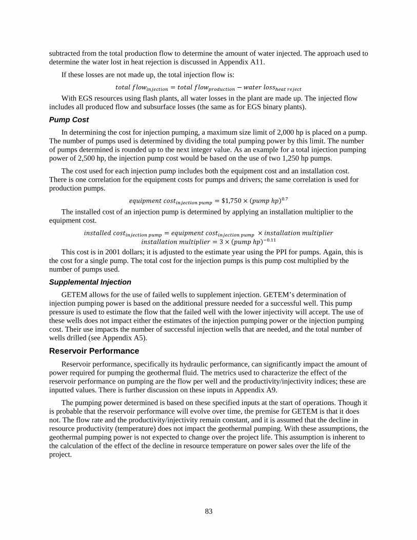
83

subtracted from the total production flow to determine the amount of water injected. The approach used to determine the water lost in heat rejection is discussed in Appendix A11.

If these losses are not made up, the total injection flow is: 𝑃𝑃𝑃𝑃𝑃𝑃𝑆𝑆𝑆𝑆 𝑓𝑓𝑆𝑆𝑃𝑃𝑃𝑃𝑓𝑓𝑛𝑛𝑝𝑝𝑛𝑛𝑎𝑎𝑛𝑛𝑓𝑓𝑔𝑔𝑛𝑛 = 𝑃𝑃𝑃𝑃𝑃𝑃𝑆𝑆𝑆𝑆 𝑓𝑓𝑆𝑆𝑃𝑃𝑃𝑃𝑝𝑝𝑝𝑝𝑔𝑔𝑓𝑓𝑓𝑓𝑎𝑎𝑛𝑛𝑓𝑓𝑔𝑔𝑛𝑛 − 𝑃𝑃𝑆𝑆𝑃𝑃𝑃𝑃𝑃𝑃 𝑆𝑆𝑃𝑃𝑆𝑆𝑆𝑆ℎ𝑛𝑛𝑝𝑝𝑛𝑛 𝑝𝑝𝑛𝑛𝑝𝑝𝑛𝑛𝑎𝑎𝑛𝑛

With EGS resources using flash plants, all water losses in the plant are made up. The injected flow includes all produced flow and subsurface losses (the same as for EGS binary plants).

Pump Cost In determining the cost for injection pumping, a maximum size limit of 2,000 hp is placed on a pump.

The number of pumps used is determined by dividing the total pumping power by this limit. The number of pumps determined is rounded up to the next integer value. As an example for a total injection pumping power of 2,500 hp, the injection pump cost would be based on the use of two 1,250 hp pumps.

The cost used for each injection pump includes both the equipment cost and an installation cost. There is one correlation for the equipment costs for pumps and drivers; the same correlation is used for production pumps.

𝑃𝑃𝑒𝑒𝑃𝑃𝑃𝑃𝑃𝑃𝑃𝑃𝑃𝑃𝑃𝑃𝑃𝑃 𝑃𝑃𝑃𝑃𝑆𝑆𝑃𝑃𝑓𝑓𝑛𝑛𝑝𝑝𝑛𝑛𝑎𝑎𝑛𝑛𝑓𝑓𝑔𝑔𝑛𝑛 𝑝𝑝𝑓𝑓𝑝𝑝𝑝𝑝 = $1,750 × (𝑃𝑃𝑃𝑃𝑃𝑃𝑃𝑃 ℎ𝑃𝑃)0.7

The installed cost of an injection pump is determined by applying an installation multiplier to the equipment cost.

𝑃𝑃𝑃𝑃𝑆𝑆𝑃𝑃𝑆𝑆𝑆𝑆𝑆𝑆𝑃𝑃𝑑𝑑 𝑃𝑃𝑃𝑃𝑆𝑆𝑃𝑃𝑓𝑓𝑛𝑛𝑝𝑝𝑛𝑛𝑎𝑎𝑛𝑛𝑓𝑓𝑔𝑔𝑛𝑛 𝑝𝑝𝑓𝑓𝑝𝑝𝑝𝑝 = 𝑃𝑃𝑒𝑒𝑃𝑃𝑃𝑃𝑃𝑃𝑃𝑃𝑃𝑃𝑃𝑃𝑃𝑃 𝑃𝑃𝑃𝑃𝑆𝑆𝑃𝑃𝑓𝑓𝑛𝑛𝑝𝑝𝑛𝑛𝑎𝑎𝑛𝑛𝑓𝑓𝑔𝑔𝑛𝑛 𝑝𝑝𝑓𝑓𝑝𝑝𝑝𝑝 × 𝑃𝑃𝑃𝑃𝑆𝑆𝑃𝑃𝑆𝑆𝑆𝑆𝑆𝑆𝑆𝑆𝑃𝑃𝑃𝑃𝑃𝑃𝑃𝑃 𝑃𝑃𝑃𝑃𝑆𝑆𝑃𝑃𝑃𝑃𝑃𝑃𝑆𝑆𝑃𝑃𝑃𝑃𝑃𝑃 𝑃𝑃𝑃𝑃𝑆𝑆𝑃𝑃𝑆𝑆𝑆𝑆𝑆𝑆𝑆𝑆𝑃𝑃𝑃𝑃𝑃𝑃𝑃𝑃 𝑃𝑃𝑃𝑃𝑆𝑆𝑃𝑃𝑃𝑃𝑃𝑃𝑆𝑆𝑃𝑃𝑃𝑃𝑃𝑃 = 3 × (𝑃𝑃𝑃𝑃𝑃𝑃𝑃𝑃 ℎ𝑃𝑃)−0.11

This cost is in 2001 dollars; it is adjusted to the estimate year using the PPI for pumps. Again, this is the cost for a single pump. The total cost for the injection pumps is this pump cost multiplied by the number of pumps used.

Supplemental Injection GETEM allows for the use of failed wells to supplement injection. GETEM’s determination of

injection pumping power is based on the additional pressure needed for a successful well. This pump pressure is used to estimate the flow that the failed well with the lower injectivity will accept. The use of these wells does not impact either the estimates of the injection pumping power or the injection pumping cost. Their use impacts the number of successful injection wells that are needed, and the total number of wells drilled (see Appendix A5).

Reservoir Performance Reservoir performance, specifically its hydraulic performance, can significantly impact the amount of

power required for pumping the geothermal fluid. The metrics used to characterize the effect of the reservoir performance on pumping are the flow per well and the productivity/injectivity indices; these are inputted values. There is further discussion on these inputs in Appendix A9.

The pumping power determined is based on these specified inputs at the start of operations. Though it is probable that the reservoir performance will evolve over time, the premise for GETEM is that it does not. The flow rate and the productivity/injectivity remain constant, and it is assumed that the decline in resource productivity (temperature) does not impact the geothermal pumping. With these assumptions, the geothermal pumping power is not expected to change over the project life. This assumption is inherent to the calculation of the effect of the decline in resource temperature on power sales over the life of the project.

84

Well Configuration An assumed configuration for both the production and injection wells is used in estimating both the

friction losses and temperature drop in a flowing well. The configuration is based upon the depth of the well, the production/injection interval size (smaller or larger diameter), and whether the production/injection interval is open or has a perforated/slotted liner.

The well configuration is based on the number of intervals (casing or liners) required in drilling the well. The possible configurations considered are shown below in Figure A-15. The designation of the number of intervals is based on the bottom injection/production interval plus the number of casing/liners installed above the bottom interval. (The conductor casing is not included in the interval count.)

3 Intervals 4 Intervals 5 Intervals

Figure A-15. Well configurations, with three, four, and five intervals, respectively.

The configuration on the left has three intervals—the surface casing, the upper casing and the production/injection interval. The configuration on the right has five intervals—the surface casing, the upper casing, the upper intermediate interval liner, the lower intermediate interval liner, and the production/injection interval. The differentiation in GETEM between a casing and a liner is that casing comes from depth back to the surface, while liners are “hung” within the well. (They are not run back to the surface.) All casing is cemented in place, as are all liners, except for that in the production/injection interval. When estimating friction losses, only intervals through which fluid flows are considered; hence, in the determination of the pumping power, the number of intervals is always the value shown in Figure A-15 less one.

The production pump is installed in the upper casing interval; to accommodate the pump, the minimum diameter in this interval is 13 5/8 inch when a pump is used.

The model defaults to a bottom hole configuration using the following logic:

• For both EGS and hydrothermal resources with binary plants, the model defaults to the larger-diameter well.

• For both EGS and hydrothermal resources with flash plants, the model defaults to the smaller-diameter well.

• Injection wells have the same diameter as production wells.

• EGS wells have perforated or slotted liners in the production/injection intervals; hydrothermal wells are open-hole in the bottom intervals.

85

Though EGS well flow rates are postulated to be less than flows from hydrothermal wells in the near term, the larger-diameter wells are used with production pumps in order to accommodate a production pump. Table A-5 below shows the defaults used by the model to define the well configuration.

Table A-5. Defaults used by GETEM to define well configuration. Depth <3 km 3-5 km >5km

# casing intervals 3 4 5

# intervals with flow 2 3 4

Bottom hole diameter larger well

Open 12.25-inch 12.25-inch 12.25-inch

Slotted liner 9.625-inch 9.625-inch 9.625-inch

Upper casing diameter larger well 13.625-inch 18.625-inch 24-inch

Bottom hole diameter smaller well

Open 8.5-inch 8.5-inch 8.5-inch

Slotted liner 7-inch 7-inch 7-inch

Upper casing diameter smaller well 9.625-inch 13.5-inch 20-inch

Length: Surface casing 800 ft 1,200 ft 1,200 ft

Length: Upper casing 80% of depth 40% of depth 30% of depth

Length: Upper liner NA 40% of depth 30% of depth

Length: Intermediate liner NA NA 30% of depth

Length: Production/injection interval 20% of depth 20% of depth 10% of depth

Again, the production pump is set in the upper casing; the maximum setting depth for an electric

submersible pump is established by the casing length for this interval. The maximum depth for a line-shaft pump is assumed to be 2,000 ft, or 610 m. (If this depth is exceeded, a warning should occur.)

Temperature Loss in Well Bore GETEM includes a simplified estimate of the temperature loss in the well bore as fluid flows up

the well. While the loss might be considered negligible in productive, shallow hydrothermal wells, it has the potential to be significant for the deep wells, especially if the wells are less productive (lower flow rates).

The method used is adapted from Ramey’s article in the Journal of Petroleum Technology (Ramey 1962); equations (1), (2), (3), and (5) in this paper are used. This methodology provides an estimated solution for the temperature loss, assuming the heat transfer from the well bore to the earth is

86

unsteady transient conduction. The calculation assumes that the sufficient time has occurred since beginning flow that the simple solution provided by Ramey can be applied. The paper suggests 1 week; GETEM uses 1 year. Each interval in the well is divided into three segments of equal length and the fluid temperature estimated at each point.

The temperature loss in the well is used in estimating the pumping power required. The production wellhead temperature determined is also used in estimating the power plant performance and cost.

An example of the estimated temperature loss in the production well is given in Figure A-16 below for two different resource temperatures, each at two different resource depths. This is indicative of how flow and depth impact the production temperature in GETEM.

Figure A-16. Estimated temperature loss in the production well.

The consequence of this temperature loss is a reduced potential to produce power. Below in Figure A-17 is the effect of a temperature loss on the ideal power at these two resource temperatures. This loss in available energy is indicative of the actual reduction in generation/sales that would occur. To offset the loss, more flow and wells would be needed.

87

Figure A-17. The effect of a well bore temperature loss on the idea power at 150 and 250°C.

A9: RESERVOIR Production Well Flow

The production well flow can have a significant influence on the LCOE determined. As shown in Figure A-18 below, this flow affects the sizes of both the plant and the well field.

Figure A-18. Production well flow rate as it affects plant size and well field size.

Though it may not be readily apparent, for a given scenario there is likely to be an optimal well flow rate. If the flow rate is too high, the effect of the increased pumping power negates the benefit of the higher flow rate per well. This is illustrated in Figure A-19 below, which shows the impact of flow on the size of the plant, the well count, and the LCOE determined for a DOE GTO–defined

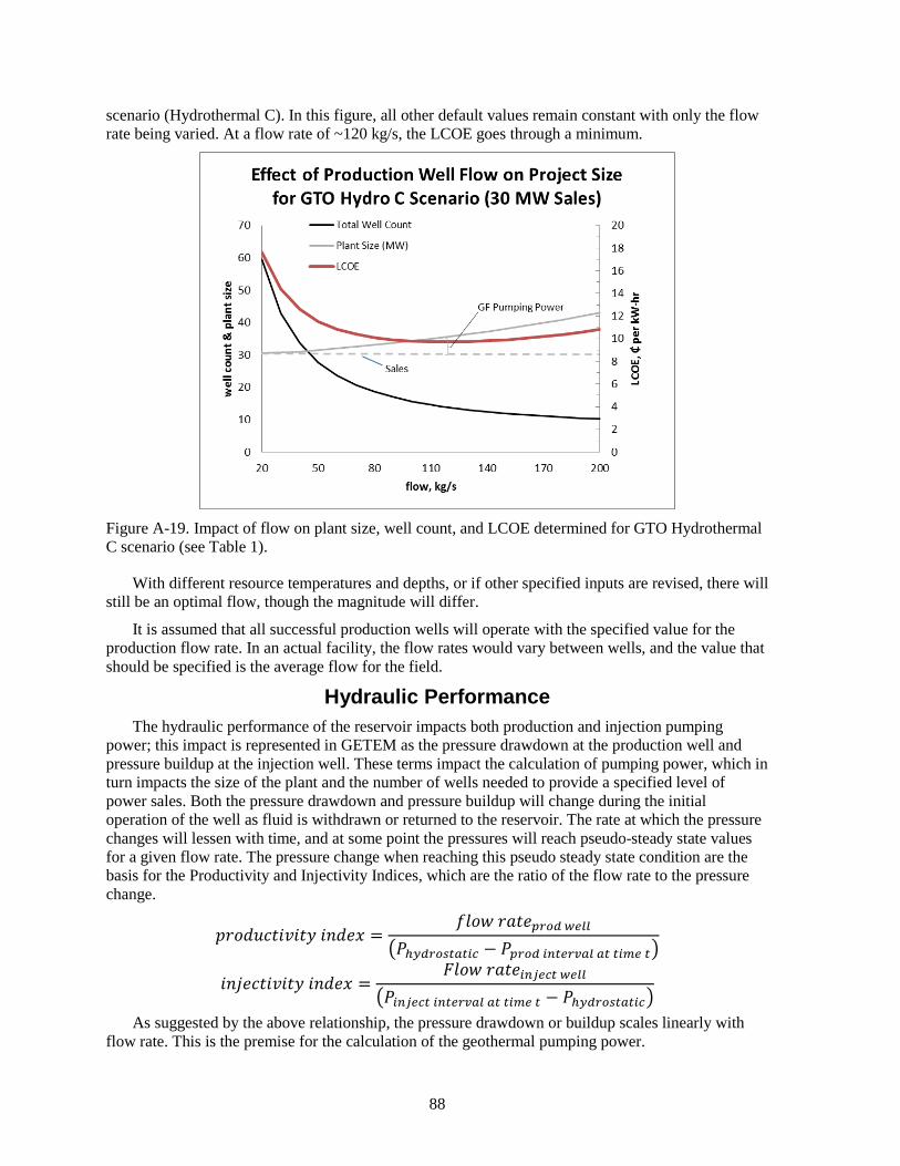
88

scenario (Hydrothermal C). In this figure, all other default values remain constant with only the flow rate being varied. At a flow rate of ~120 kg/s, the LCOE goes through a minimum.

Figure A-19. Impact of flow on plant size, well count, and LCOE determined for GTO Hydrothermal C scenario (see Table 1).

With different resource temperatures and depths, or if other specified inputs are revised, there will still be an optimal flow, though the magnitude will differ.

It is assumed that all successful production wells will operate with the specified value for the production flow rate. In an actual facility, the flow rates would vary between wells, and the value that should be specified is the average flow for the field.

Hydraulic Performance The hydraulic performance of the reservoir impacts both production and injection pumping

power; this impact is represented in GETEM as the pressure drawdown at the production well and pressure buildup at the injection well. These terms impact the calculation of pumping power, which in turn impacts the size of the plant and the number of wells needed to provide a specified level of power sales. Both the pressure drawdown and pressure buildup will change during the initial operation of the well as fluid is withdrawn or returned to the reservoir. The rate at which the pressure changes will lessen with time, and at some point the pressures will reach pseudo-steady state values for a given flow rate. The pressure change when reaching this pseudo steady state condition are the basis for the Productivity and Injectivity Indices, which are the ratio of the flow rate to the pressure change.

𝑃𝑃𝑃𝑃𝑃𝑃𝑑𝑑𝑃𝑃𝑃𝑃𝑃𝑃𝑃𝑃𝑙𝑙𝑃𝑃𝑃𝑃𝑐𝑐 𝑃𝑃𝑃𝑃𝑑𝑑𝑃𝑃𝐼𝐼 =𝑓𝑓𝑆𝑆𝑃𝑃𝑃𝑃 𝑃𝑃𝑆𝑆𝑃𝑃𝑃𝑃𝑝𝑝𝑝𝑝𝑔𝑔𝑓𝑓 𝑤𝑤𝑛𝑛𝑓𝑓𝑓𝑓

�𝑃𝑃ℎ𝑎𝑎𝑓𝑓𝑝𝑝𝑔𝑔𝑑𝑑𝑛𝑛𝑝𝑝𝑛𝑛𝑓𝑓𝑎𝑎 − 𝑃𝑃𝑝𝑝𝑝𝑝𝑔𝑔𝑓𝑓 𝑓𝑓𝑛𝑛𝑛𝑛𝑛𝑛𝑝𝑝𝑎𝑎𝑝𝑝𝑓𝑓 𝑝𝑝𝑛𝑛 𝑛𝑛𝑓𝑓𝑝𝑝𝑛𝑛 𝑛𝑛�

𝑃𝑃𝑃𝑃𝑝𝑝𝑃𝑃𝑃𝑃𝑃𝑃𝑃𝑃𝑙𝑙𝑃𝑃𝑃𝑃𝑐𝑐 𝑃𝑃𝑃𝑃𝑑𝑑𝑃𝑃𝐼𝐼 =𝐶𝐶𝑆𝑆𝑃𝑃𝑃𝑃 𝑃𝑃𝑆𝑆𝑃𝑃𝑃𝑃𝑓𝑓𝑛𝑛𝑝𝑝𝑛𝑛𝑎𝑎𝑛𝑛 𝑤𝑤𝑛𝑛𝑓𝑓𝑓𝑓

�𝑃𝑃𝑓𝑓𝑛𝑛𝑝𝑝𝑛𝑛𝑎𝑎𝑛𝑛 𝑓𝑓𝑛𝑛𝑛𝑛𝑛𝑛𝑝𝑝𝑎𝑎𝑝𝑝𝑓𝑓 𝑝𝑝𝑛𝑛 𝑛𝑛𝑓𝑓𝑝𝑝𝑛𝑛 𝑛𝑛 − 𝑃𝑃ℎ𝑎𝑎𝑓𝑓𝑝𝑝𝑔𝑔𝑑𝑑𝑛𝑛𝑝𝑝𝑛𝑛𝑓𝑓𝑎𝑎�

As suggested by the above relationship, the pressure drawdown or buildup scales linearly with flow rate. This is the premise for the calculation of the geothermal pumping power.

89

These indices are not calculated; they are specified inputs to the model. The values for these indices will vary between resources, as well as among wells at a given resource. GETEM cannot account for this variability; the values specified are to be representative of the scenario being defined and evaluated.

The default is to use equivalent productivity and injectivity indices for a given resource. The default value used in the model for hydrothermal resources is taken from the ERPI study (EPRI 1996; 2,500 lb/hr-psi). It is probable that in commercial plants, the magnitude of the PP’s and II’s vary inversely with the resource temperature; for power production from lower temperature resources to be economically viable, the resources must be more productive.

The impact of the productivity and injectivity index used is shown in Figure A-20. Again, this figure is based on the same DOE GTO scenario used in Figure A-19, “Hydro C.” The variation in the LCOE determined as a function of flow rate for three scenarios for the productivity and injectivity index is shown (including the default value, 50% of default, and 150% of default). For all three PI/II values considered, the LCOE goes through a minimum. That minimum value is identified with the vertical arrows.

Figure A-20. Effect of hydraulic performance and flow rate on LCOE for the “Hydrothermal C”.

Because there is minimal information that can be used to establish representative values for these inputs for EGS resources, it has been assumed that the EGS reservoir created with have both thermal and hydraulic performance equivalent to that of a hydrothermal resource, but at the lower specified EGS well flow rates.

Resource Productivity GETEM does not model the performance of the reservoir. Rather, it models the impact of

reservoir performance on the power sales and the required LCOE. Based on the historical operation of existing geothermal facilities, there is an expectation that, over time, the productivity of the reservoir will decline. This decline in productivity will manifest as a decreasing temperature, pressure, and/or flow rate. GETEM characterizes the decrease in productivity using a declining resource temperature.

Temperature was selected as the metric for assessing the effect of declining productivity because

• nearly all plants experience temperature decline over time

90

• plant performance is typically more sensitive to changes in temperature than changes in flow

• the effect of temperature on generation can be estimated in a straightforward manner

• in some instances, flow rates increase as operators attempt to offset temperature decline.

With the selection of temperature as the metric for depicting declining productivity, it is inherent to the calculations that the geothermal flow rate remains constant over the life of the project.

Temperature Decline The decline in the resource temperature with time is specified as an annual decline

𝑇𝑇𝑛𝑛 = 𝑇𝑇𝑓𝑓𝑛𝑛𝑓𝑓𝑛𝑛𝑓𝑓𝑝𝑝𝑓𝑓�1 − 𝜗𝜗𝑔𝑔𝑓𝑓�𝑛𝑛

, where

T is the temperature of the geothermal fluid

n is the point in time (in years)

𝜗𝜗𝑔𝑔𝑓𝑓 is the annual decline rate.

The effect of the decline rate on the produced temperature over time is shown in Figure A-21 below.

Figure A-21. The effect of the decline rate on the produced temperature over time.

The default values used for the decline rate are based on an evaluation of historical operating data reported to the Nevada Division of Minerals by the geothermal operators (Hanson 2014). The decline rates for the Nevada binary plants typically approach the 0.5% shown in Figure A-21. Similar decline rates were found for flash plants, though there are a limited number of these plants in Nevada. Some plants experienced rates approaching or exceeding the 1% shown. This was often for an abbreviated period, with the rate of decline being mitigated by changing the injection strategy.

Available Energy Available energy, or exergy, is a measure of the work that can be done in bringing a fluid into

equilibrium with a “dead-state” condition (taken to be the ambient) using ideal, reversible processes. This represents that maximum work that could be done by an ideal conversion system. The available energy is defined as

𝑆𝑆��𝑃 = (ℎ − ℎ𝑔𝑔) − 𝑇𝑇𝑔𝑔(𝑆𝑆 − 𝑆𝑆𝑔𝑔) , where 𝑆𝑆��𝑃 is the specific available energy of the geothermal fluid (per unit mass)

91

h is the enthalpy of the geothermal fluid

ho is the enthalpy of the geothermal fluid at the ambient conditions

To is the ambient temperature

s is the entropy of the geothermal fluid

so is the entropy of the geothermal fluid at the ambient conditions.

The dead-state condition is taken to be the ambient condition corresponding to a mean or average annual temperature. In GETEM, the ambient temperature for binary plants is 10°C; this value cannot be revised, as it is integral to GETEM’s determination of the air-cooled binary plant cost. (In the U.S., the average ambient temperature is ~11° to 12°C.) For flash steam plants, a design wet-bulb temperature is specified, which is used as the ambient condition when determining the available energy. Once ambient conditions are fixed, available energy is effectively a property of the geothermal fluid.

Second Law Efficiency The brine effectiveness and the second law efficiency are used as plant performance metrics. The

brine effectiveness is also referred to as the specific power output and the brine utilization factor. It is the net plant output per unit mass flow:

𝑏𝑏𝑃𝑃𝑃𝑃𝑃𝑃𝑃𝑃 𝑃𝑃𝑓𝑓𝑓𝑓𝑃𝑃𝑃𝑃𝑃𝑃𝑃𝑃𝑙𝑙𝑃𝑃𝑃𝑃𝑃𝑃𝑆𝑆𝑆𝑆 =(𝑃𝑃𝑃𝑃𝑃𝑃𝑃𝑃𝑃𝑃𝑆𝑆𝑃𝑃𝑃𝑃𝑃𝑃 𝑃𝑃𝑃𝑃𝑃𝑃𝑃𝑃𝑃𝑃𝑃𝑃 − 𝑃𝑃𝑆𝑆𝑆𝑆𝑃𝑃𝑃𝑃 𝑃𝑃𝑆𝑆𝑃𝑃𝑆𝑆𝑆𝑆𝑃𝑃𝑃𝑃𝑃𝑃𝑃𝑃 𝑆𝑆𝑃𝑃𝑆𝑆𝑑𝑑)

𝑃𝑃𝑔𝑔𝑓𝑓

In this definition, net plant output is exclusive of the geothermal pumping. This is a fundamental definition used throughout GETEM’s calculations. It is the basis for establishing both the plant cost and the size of the well field required.

Unlike the thermal efficiency, which is a measure of how efficiently the extracted heat is converted to power, the second law efficiency is a measure of how efficiently a plant uses a given mass flow of geothermal fluid to produce electrical power. The cost of the power plant varies directly with this efficiency, while the amount of geothermal fluid required to produce a given level of power sales varies indirectly. The second law efficiency is the ratio of brine effectiveness to the available energy:

2 𝑛𝑛𝑓𝑓𝑆𝑆𝑆𝑆𝑃𝑃 𝑃𝑃𝑓𝑓𝑓𝑓𝑃𝑃𝑃𝑃𝑃𝑃𝑃𝑃𝑃𝑃𝑃𝑃𝑐𝑐, 𝜂𝜂𝐼𝐼𝐼𝐼 =𝑏𝑏𝑃𝑃𝑃𝑃𝑃𝑃𝑃𝑃 𝑃𝑃𝑓𝑓𝑓𝑓𝑃𝑃𝑃𝑃𝑃𝑃𝑃𝑃𝑙𝑙𝑃𝑃𝑃𝑃𝑃𝑃𝑆𝑆𝑆𝑆

𝑆𝑆��𝑃

At a constant geothermal flow rate, a power plant typically achieves its maximum second law efficiency when operating at its design conditions (geothermal and air temperatures). Though this efficiency may initially increase slightly with increasing resource temperature, at some elevated temperature this conversion efficiency will decrease. The plant output will continue to increase with increasing temperature because the available energy is also increasing; however, the increase in plant output will lag behind the increase in available energy because of the second law efficiency decline. If the resource temperature decreases, both the second law efficiency and available energy decrease; the impact on power will be greater than would be expected by considering the change in available energy.

The second law efficiency is also impacted by changes in the ambient temperature. In GETEM’s calculations for binary plants, the ambient temperature is held constant. Its effect on performance, however, is captured in the net capacity factor that is used. This capacity factor accounts for both plant availability and the effect of the ambient temperature on power generation throughout the year (see Appendix A1).

92

GETEM determines the second law efficiency based on the geothermal conditions at the start of operation. In estimating power generation, this efficiency is corrected to account for changes in the geothermal temperature using a correlation that is based on changes in the Carnot efficiency. The Carnot efficiency is defined as:

𝐿𝐿𝑆𝑆𝑃𝑃𝑃𝑃𝑃𝑃𝑃𝑃 𝑃𝑃𝑓𝑓𝑓𝑓𝑃𝑃𝑃𝑃𝑃𝑃𝑃𝑃𝑃𝑃𝑃𝑃𝑐𝑐 = 1 −𝑇𝑇0𝑇𝑇

In this relationship, To is the assumed ambient temperature (kept fixed), and T is the geothermal temperature at a point in time; both are absolute temperatures in either °K or °R. The relationships between the second law efficiency and the Carnot efficiency that are used for both air-cooled binary and flash steam plants are based upon modeling that has been done of the performance of plants operating with fixed equipment (size and performance) at off-design conditions.

The following are the relationships used to determine how temperature decline (as represented by the Carnot efficiency) impacts the second law efficiency:

Binary Plants

𝑃𝑃𝑓𝑓𝑓𝑓𝑃𝑃𝑓𝑓𝑓𝑓𝑓𝑓𝑛𝑛𝑑𝑑𝑓𝑓𝑔𝑔𝑛𝑛

= −10.956 �𝐿𝐿𝑆𝑆𝑃𝑃𝑃𝑃𝑃𝑃𝑃𝑃 𝑃𝑃𝑓𝑓𝑓𝑓

𝐿𝐿𝑆𝑆𝑃𝑃𝑃𝑃𝑃𝑃𝑃𝑃 𝑃𝑃𝑓𝑓𝑓𝑓𝑓𝑓𝑛𝑛𝑓𝑓𝑛𝑛𝑓𝑓𝑝𝑝𝑓𝑓�2

+ 22.422 �𝐿𝐿𝑆𝑆𝑃𝑃𝑃𝑃𝑃𝑃𝑃𝑃 𝑃𝑃𝑓𝑓𝑓𝑓

𝐿𝐿𝑆𝑆𝑃𝑃𝑃𝑃𝑃𝑃𝑃𝑃 𝑃𝑃𝑓𝑓𝑓𝑓𝑓𝑓𝑛𝑛𝑓𝑓𝑛𝑛𝑓𝑓𝑝𝑝𝑓𝑓� − 10.466

Dual-Flash Steam Plants, T> 210°C

𝑃𝑃𝑓𝑓𝑓𝑓𝑃𝑃𝑓𝑓𝑓𝑓𝑓𝑓𝑛𝑛𝑑𝑑𝑓𝑓𝑔𝑔𝑛𝑛

= −9.5604 �𝐿𝐿𝑆𝑆𝑃𝑃𝑃𝑃𝑃𝑃𝑃𝑃 𝑃𝑃𝑓𝑓𝑓𝑓

𝐿𝐿𝑆𝑆𝑃𝑃𝑃𝑃𝑃𝑃𝑃𝑃 𝑃𝑃𝑓𝑓𝑓𝑓𝑓𝑓𝑛𝑛𝑓𝑓𝑛𝑛𝑓𝑓𝑝𝑝𝑓𝑓�2

+ 19.388 �𝐿𝐿𝑆𝑆𝑃𝑃𝑃𝑃𝑃𝑃𝑃𝑃 𝑃𝑃𝑓𝑓𝑓𝑓

𝐿𝐿𝑆𝑆𝑃𝑃𝑃𝑃𝑃𝑃𝑃𝑃 𝑃𝑃𝑓𝑓𝑓𝑓𝑓𝑓𝑛𝑛𝑓𝑓𝑛𝑛𝑓𝑓𝑝𝑝𝑓𝑓� − 8.8276

Dual-Flash Steam Plants, T< 210°C

𝑃𝑃𝑓𝑓𝑓𝑓𝑃𝑃𝑓𝑓𝑓𝑓𝑓𝑓𝑛𝑛𝑑𝑑𝑓𝑓𝑔𝑔𝑛𝑛

= −10.559 �𝐿𝐿𝑆𝑆𝑃𝑃𝑃𝑃𝑃𝑃𝑃𝑃 𝑃𝑃𝑓𝑓𝑓𝑓

𝐿𝐿𝑆𝑆𝑃𝑃𝑃𝑃𝑃𝑃𝑃𝑃 𝑃𝑃𝑓𝑓𝑓𝑓𝑓𝑓𝑛𝑛𝑓𝑓𝑛𝑛𝑓𝑓𝑝𝑝𝑓𝑓�2

+ 21.683 �𝐿𝐿𝑆𝑆𝑃𝑃𝑃𝑃𝑃𝑃𝑃𝑃 𝑃𝑃𝑓𝑓𝑓𝑓

𝐿𝐿𝑆𝑆𝑃𝑃𝑃𝑃𝑃𝑃𝑃𝑃 𝑃𝑃𝑓𝑓𝑓𝑓𝑓𝑓𝑛𝑛𝑓𝑓𝑛𝑛𝑓𝑓𝑝𝑝𝑓𝑓� − 10.124

Single-Flash Steam Plants, T> 240°C

𝑃𝑃𝑓𝑓𝑓𝑓𝑃𝑃𝑓𝑓𝑓𝑓𝑓𝑓𝑛𝑛𝑑𝑑𝑓𝑓𝑔𝑔𝑛𝑛

= −11.42747 �𝐿𝐿𝑆𝑆𝑃𝑃𝑃𝑃𝑃𝑃𝑃𝑃 𝑃𝑃𝑓𝑓𝑓𝑓

𝐿𝐿𝑆𝑆𝑃𝑃𝑃𝑃𝑃𝑃𝑃𝑃 𝑃𝑃𝑓𝑓𝑓𝑓𝑓𝑓𝑛𝑛𝑓𝑓𝑛𝑛𝑓𝑓𝑝𝑝𝑓𝑓�2

+ 22.89446 �𝐿𝐿𝑆𝑆𝑃𝑃𝑃𝑃𝑃𝑃𝑃𝑃 𝑃𝑃𝑓𝑓𝑓𝑓

𝐿𝐿𝑆𝑆𝑃𝑃𝑃𝑃𝑃𝑃𝑃𝑃 𝑃𝑃𝑓𝑓𝑓𝑓𝑓𝑓𝑛𝑛𝑓𝑓𝑛𝑛𝑓𝑓𝑝𝑝𝑓𝑓� − 10.467

Single-Flash Steam Plants, T< 240°C

𝑃𝑃𝑓𝑓𝑓𝑓𝑃𝑃𝑓𝑓𝑓𝑓𝑓𝑓𝑛𝑛𝑑𝑑𝑓𝑓𝑔𝑔𝑛𝑛

= −10.06859 �𝐿𝐿𝑆𝑆𝑃𝑃𝑃𝑃𝑃𝑃𝑃𝑃 𝑃𝑃𝑓𝑓𝑓𝑓

𝐿𝐿𝑆𝑆𝑃𝑃𝑃𝑃𝑃𝑃𝑃𝑃 𝑃𝑃𝑓𝑓𝑓𝑓𝑓𝑓𝑛𝑛𝑓𝑓𝑛𝑛𝑓𝑓𝑝𝑝𝑓𝑓�2

+ 20.13903 �𝐿𝐿𝑆𝑆𝑃𝑃𝑃𝑃𝑃𝑃𝑃𝑃 𝑃𝑃𝑓𝑓𝑓𝑓

𝐿𝐿𝑆𝑆𝑃𝑃𝑃𝑃𝑃𝑃𝑃𝑃 𝑃𝑃𝑓𝑓𝑓𝑓𝑓𝑓𝑛𝑛𝑓𝑓𝑛𝑛𝑓𝑓𝑝𝑝𝑓𝑓� − 9.07044

The flash steam plants have relationships that are functions of temperature because, as the resource temperature declines, at some point the lowest flash pressure can reach 1 atm. It is assumed that the operator will take steps to assure the plant does not operate with sub-atmospheric flash pressures.

The effect that the temperature decline has on conversion efficiency used is illustrated in Figure A-22.

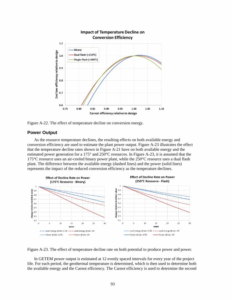
93

Figure A-22. The effect of temperature decline on conversion energy.

Power Output As the resource temperature declines, the resulting effects on both available energy and

conversion efficiency are used to estimate the plant power output. Figure A-23 illustrates the effect that the temperature decline rates shown in Figure A-21 have on both available energy and the estimated power generation for a 175° and 250°C resources. In Figure A-23, it is assumed that the 175°C resource uses an air-cooled binary power plant, while the 250°C resource uses a dual flash plant. The difference between the available energy (dashed lines) and the power (solid lines) represents the impact of the reduced conversion efficiency as the temperature declines.

Figure A-23. The effect of temperature decline rate on both potential to produce power and power.

In GETEM power output is estimated at 12 evenly spaced intervals for every year of the project life. For each period, the geothermal temperature is determined, which is then used to determine both the available energy and the Carnot efficiency. The Carnot efficiency is used to determine the second

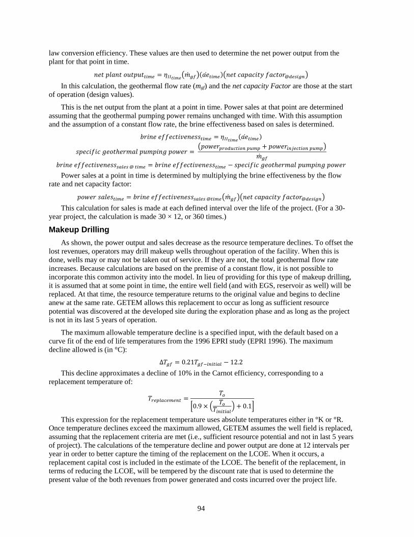
94

law conversion efficiency. These values are then used to determine the net power output from the plant for that point in time.

𝑃𝑃𝑃𝑃𝑃𝑃 𝑃𝑃𝑆𝑆𝑆𝑆𝑃𝑃𝑃𝑃 𝑃𝑃𝑃𝑃𝑃𝑃𝑃𝑃𝑃𝑃𝑃𝑃𝑛𝑛𝑓𝑓𝑝𝑝𝑛𝑛 = 𝜂𝜂𝐼𝐼𝐼𝐼𝑠𝑠𝑖𝑖𝑡𝑡𝑒𝑒���𝑃𝑔𝑔𝑓𝑓�(𝑆𝑆��𝑃𝑛𝑛𝑓𝑓𝑝𝑝𝑛𝑛)�𝑃𝑃𝑃𝑃𝑃𝑃 𝑃𝑃𝑆𝑆𝑃𝑃𝑆𝑆𝑃𝑃𝑃𝑃𝑃𝑃𝑐𝑐 𝑓𝑓𝑆𝑆𝑃𝑃𝑃𝑃𝑃𝑃𝑃𝑃@𝑓𝑓𝑛𝑛𝑑𝑑𝑓𝑓𝑔𝑔𝑛𝑛�

In this calculation, the geothermal flow rate (mgf) and the net capacity Factor are those at the start of operation (design values).

This is the net output from the plant at a point in time. Power sales at that point are determined assuming that the geothermal pumping power remains unchanged with time. With this assumption and the assumption of a constant flow rate, the brine effectiveness based on sales is determined.

𝑏𝑏𝑃𝑃𝑃𝑃𝑃𝑃𝑃𝑃 𝑃𝑃𝑓𝑓𝑓𝑓𝑃𝑃𝑃𝑃𝑃𝑃𝑃𝑃𝑙𝑙𝑃𝑃𝑃𝑃𝑃𝑃𝑆𝑆𝑆𝑆𝑛𝑛𝑓𝑓𝑝𝑝𝑛𝑛 = 𝜂𝜂𝐼𝐼𝐼𝐼𝑠𝑠𝑖𝑖𝑡𝑡𝑒𝑒(𝑆𝑆��𝑃𝑛𝑛𝑓𝑓𝑝𝑝𝑛𝑛)

𝑆𝑆𝑃𝑃𝑃𝑃𝑃𝑃𝑃𝑃𝑓𝑓𝑃𝑃𝑃𝑃 𝑃𝑃𝑃𝑃𝑃𝑃𝑃𝑃ℎ𝑃𝑃𝑃𝑃𝑃𝑃𝑆𝑆𝑆𝑆 𝑃𝑃𝑃𝑃𝑃𝑃𝑃𝑃𝑃𝑃𝑃𝑃𝑃𝑃 𝑃𝑃𝑃𝑃𝑃𝑃𝑃𝑃𝑃𝑃 = �𝑃𝑃𝑃𝑃𝑃𝑃𝑃𝑃𝑃𝑃𝑝𝑝𝑝𝑝𝑔𝑔𝑓𝑓𝑓𝑓𝑎𝑎𝑛𝑛𝑓𝑓𝑔𝑔𝑛𝑛 𝑝𝑝𝑓𝑓𝑝𝑝𝑝𝑝 + 𝑃𝑃𝑃𝑃𝑃𝑃𝑃𝑃𝑃𝑃𝑓𝑓𝑛𝑛𝑝𝑝𝑛𝑛𝑎𝑎𝑛𝑛𝑓𝑓𝑔𝑔𝑛𝑛 𝑝𝑝𝑓𝑓𝑝𝑝𝑝𝑝�

��𝑃𝑔𝑔𝑓𝑓

𝑏𝑏𝑃𝑃𝑃𝑃𝑃𝑃𝑃𝑃 𝑃𝑃𝑓𝑓𝑓𝑓𝑃𝑃𝑃𝑃𝑃𝑃𝑃𝑃𝑙𝑙𝑃𝑃𝑃𝑃𝑃𝑃𝑆𝑆𝑆𝑆𝑑𝑑𝑝𝑝𝑓𝑓𝑛𝑛𝑑𝑑 @ 𝑛𝑛𝑓𝑓𝑝𝑝𝑛𝑛 = 𝑏𝑏𝑃𝑃𝑃𝑃𝑃𝑃𝑃𝑃 𝑃𝑃𝑓𝑓𝑓𝑓𝑃𝑃𝑃𝑃𝑃𝑃𝑃𝑃𝑙𝑙𝑃𝑃𝑃𝑃𝑃𝑃𝑆𝑆𝑆𝑆𝑛𝑛𝑓𝑓𝑝𝑝𝑛𝑛 − 𝑆𝑆𝑃𝑃𝑃𝑃𝑃𝑃𝑃𝑃𝑓𝑓𝑃𝑃𝑃𝑃 𝑃𝑃𝑃𝑃𝑃𝑃𝑃𝑃ℎ𝑃𝑃𝑃𝑃𝑃𝑃𝑆𝑆𝑆𝑆 𝑃𝑃𝑃𝑃𝑃𝑃𝑃𝑃𝑃𝑃𝑃𝑃𝑃𝑃 𝑃𝑃𝑃𝑃𝑃𝑃𝑃𝑃𝑃𝑃 Power sales at a point in time is determined by multiplying the brine effectiveness by the flow

rate and net capacity factor:

𝑃𝑃𝑃𝑃𝑃𝑃𝑃𝑃𝑃𝑃 𝑆𝑆𝑆𝑆𝑆𝑆𝑃𝑃𝑆𝑆𝑛𝑛𝑓𝑓𝑝𝑝𝑛𝑛 = 𝑏𝑏𝑃𝑃𝑃𝑃𝑃𝑃𝑃𝑃 𝑃𝑃𝑓𝑓𝑓𝑓𝑃𝑃𝑃𝑃𝑃𝑃𝑃𝑃𝑙𝑙𝑃𝑃𝑃𝑃𝑃𝑃𝑆𝑆𝑆𝑆𝑑𝑑𝑝𝑝𝑓𝑓𝑛𝑛𝑑𝑑 @𝑛𝑛𝑓𝑓𝑝𝑝𝑛𝑛���𝑃𝑔𝑔𝑓𝑓��𝑃𝑃𝑃𝑃𝑃𝑃 𝑃𝑃𝑆𝑆𝑃𝑃𝑆𝑆𝑃𝑃𝑃𝑃𝑃𝑃𝑐𝑐 𝑓𝑓𝑆𝑆𝑃𝑃𝑃𝑃𝑃𝑃𝑃𝑃@𝑓𝑓𝑛𝑛𝑑𝑑𝑓𝑓𝑔𝑔𝑛𝑛� This calculation for sales is made at each defined interval over the life of the project. (For a 30-

year project, the calculation is made 30 × 12, or 360 times.)

Makeup Drilling As shown, the power output and sales decrease as the resource temperature declines. To offset the

lost revenues, operators may drill makeup wells throughout operation of the facility. When this is done, wells may or may not be taken out of service. If they are not, the total geothermal flow rate increases. Because calculations are based on the premise of a constant flow, it is not possible to incorporate this common activity into the model. In lieu of providing for this type of makeup drilling, it is assumed that at some point in time, the entire well field (and with EGS, reservoir as well) will be replaced. At that time, the resource temperature returns to the original value and begins to decline anew at the same rate. GETEM allows this replacement to occur as long as sufficient resource potential was discovered at the developed site during the exploration phase and as long as the project is not in its last 5 years of operation.

The maximum allowable temperature decline is a specified input, with the default based on a curve fit of the end of life temperatures from the 1996 EPRI study (EPRI 1996). The maximum decline allowed is (in °C):

∆𝑇𝑇𝑔𝑔𝑓𝑓 = 0.21𝑇𝑇𝑔𝑔𝑓𝑓−𝑓𝑓𝑛𝑛𝑓𝑓𝑛𝑛𝑓𝑓𝑝𝑝𝑓𝑓 − 12.2

This decline approximates a decline of 10% in the Carnot efficiency, corresponding to a replacement temperature of:

𝑇𝑇𝑝𝑝𝑛𝑛𝑝𝑝𝑓𝑓𝑝𝑝𝑎𝑎𝑛𝑛𝑝𝑝𝑛𝑛𝑛𝑛𝑛𝑛 =𝑇𝑇𝑔𝑔

�0.9 × � 𝑇𝑇𝑔𝑔𝑇𝑇𝑓𝑓𝑛𝑛𝑓𝑓𝑛𝑛𝑓𝑓𝑝𝑝𝑓𝑓

� + 0.1�

This expression for the replacement temperature uses absolute temperatures either in °K or °R. Once temperature declines exceed the maximum allowed, GETEM assumes the well field is replaced, assuming that the replacement criteria are met (i.e., sufficient resource potential and not in last 5 years of project). The calculations of the temperature decline and power output are done at 12 intervals per year in order to better capture the timing of the replacement on the LCOE. When it occurs, a replacement capital cost is included in the estimate of the LCOE. The benefit of the replacement, in terms of reducing the LCOE, will be tempered by the discount rate that is used to determine the present value of the both revenues from power generated and costs incurred over the project life.

95

The well field replacement costs include the following: 𝑃𝑃𝑃𝑃𝑃𝑃𝑆𝑆𝑆𝑆𝑃𝑃𝑃𝑃𝑃𝑃𝑃𝑃𝑃𝑃𝑃𝑃 𝑃𝑃𝑃𝑃𝑆𝑆𝑃𝑃

= (𝑃𝑃𝑃𝑃𝑃𝑃𝑑𝑑𝑃𝑃𝑃𝑃𝑃𝑃𝑃𝑃𝑃𝑃𝑃𝑃 𝑃𝑃𝑃𝑃𝑆𝑆𝑆𝑆𝑎𝑎𝑔𝑔𝑓𝑓𝑛𝑛𝑛𝑛 + 𝑆𝑆𝑃𝑃𝑆𝑆𝑃𝑃𝑃𝑃 𝑃𝑃𝑃𝑃𝑆𝑆𝑆𝑆𝑆𝑆)× (𝑑𝑑𝑃𝑃𝑃𝑃𝑆𝑆𝑆𝑆𝑃𝑃𝑃𝑃𝑃𝑃 𝑃𝑃𝑃𝑃𝑆𝑆𝑃𝑃 + 𝑆𝑆𝑃𝑃𝑃𝑃𝑃𝑃𝑃𝑃𝑆𝑆𝑆𝑆𝑃𝑃𝑃𝑃𝑃𝑃𝑃𝑃 𝑃𝑃𝑃𝑃𝑆𝑆𝑃𝑃)𝑝𝑝𝑝𝑝𝑔𝑔𝑓𝑓𝑓𝑓𝑎𝑎𝑛𝑛𝑓𝑓𝑔𝑔𝑛𝑛 𝑤𝑤𝑛𝑛𝑓𝑓𝑓𝑓 + 𝑃𝑃𝑃𝑃𝑝𝑝𝑃𝑃𝑃𝑃𝑃𝑃𝑃𝑃𝑃𝑃𝑃𝑃 𝑃𝑃𝑃𝑃𝑆𝑆𝑆𝑆𝑎𝑎𝑔𝑔𝑓𝑓𝑛𝑛𝑛𝑛× (𝑑𝑑𝑃𝑃𝑃𝑃𝑆𝑆𝑆𝑆𝑃𝑃𝑃𝑃𝑃𝑃 𝑃𝑃𝑃𝑃𝑆𝑆𝑃𝑃 + 𝑆𝑆𝑃𝑃𝑃𝑃𝑃𝑃𝑃𝑃𝑆𝑆𝑆𝑆𝑃𝑃𝑃𝑃𝑃𝑃𝑃𝑃 𝑃𝑃𝑃𝑃𝑆𝑆𝑃𝑃)𝑓𝑓𝑛𝑛𝑝𝑝𝑛𝑛𝑎𝑎𝑛𝑛𝑓𝑓𝑔𝑔𝑛𝑛 𝑤𝑤𝑛𝑛𝑓𝑓𝑓𝑓+ 𝑆𝑆𝑃𝑃𝑃𝑃𝑓𝑓𝑆𝑆𝑃𝑃𝑃𝑃 𝑃𝑃𝑒𝑒𝑃𝑃𝑃𝑃𝑃𝑃𝑃𝑃𝑃𝑃𝑃𝑃𝑃𝑃 𝑃𝑃𝑃𝑃𝑆𝑆𝑃𝑃𝑝𝑝𝑝𝑝𝑔𝑔𝑓𝑓𝑓𝑓𝑎𝑎𝑛𝑛𝑓𝑓𝑔𝑔𝑛𝑛 & 𝑓𝑓𝑛𝑛𝑝𝑝𝑛𝑛𝑎𝑎𝑛𝑛𝑓𝑓𝑔𝑔𝑛𝑛 𝑤𝑤𝑛𝑛𝑓𝑓𝑓𝑓 + 𝑃𝑃𝑃𝑃𝑃𝑃𝑃𝑃 𝑃𝑃𝑃𝑃𝑆𝑆𝑃𝑃𝑝𝑝𝑝𝑝𝑔𝑔𝑓𝑓𝑓𝑓𝑎𝑎𝑛𝑛𝑓𝑓𝑔𝑔𝑛𝑛 𝑤𝑤𝑛𝑛𝑓𝑓𝑓𝑓𝑑𝑑+ 𝑃𝑃𝑃𝑃𝑑𝑑𝑃𝑃𝑃𝑃𝑃𝑃𝑃𝑃𝑃𝑃 𝑃𝑃𝑃𝑃𝑆𝑆𝑃𝑃

The production well count is the number of successful production wells required; the injection well count is the number of wells used for injection. This count includes any failed wells that are used to supplement injection. If failed wells are not used to supplement injection, the injection well count is the number of successful injection wells required. Indirect costs are determined using the same approach used in determining pre-operation capital costs. Overnight capital cost estimates or inputs are used, with no inflation applied. Makeup drilling is considered a replacement capital cost with the 5-year MACRS depreciation schedule applied.

Injection pumps (if used) are not replaced; they are assumed to be located at the power plant. Leasing and permitting costs are also not included in the replacement costs; it is assumed those costs are incurred at the beginning of the project.

Application of Approach This approach for estimating power was applied to production data from operating facilities to

assess whether the estimates being provided could be considered reasonable.

Binary Facility The basic approach used to estimate the impact of resource temperature decline on power

production in GETETM was used to estimate the power production from an operating facility over an extended period of operation. The estimated output was based upon the flow rate, resource temperature, and power output taken early in the plant’s operation once flow rate had stabilized. For this calculation, the average ambient air temperature used was based on data from a nearby weather station. The geothermal temperature after a period of 13 years of operation was used to establish an annual decline rate of ~0.7%. This decline rate, the initial conditions, and a net capacity factor of 95% was used to estimate the power generation over the 13 years. That estimate is shown below in Figure A-24 along with the reported generation. The fluctuations in the reported power represent the changes in power generation occurring from summer to winter. The estimated value shown does not have those fluctuations because of the constant ambient temperature used when determining the available energy. (The variation in the estimated generation is due to the changes in the number of days in between months.)

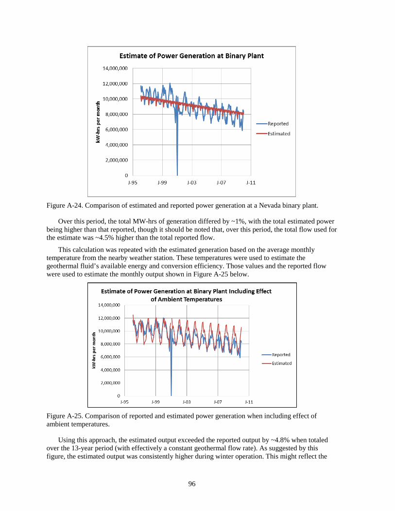
96

Figure A-24. Comparison of estimated and reported power generation at a Nevada binary plant.

Over this period, the total MW-hrs of generation differed by ~1%, with the total estimated power being higher than that reported, though it should be noted that, over this period, the total flow used for the estimate was ~4.5% higher than the total reported flow.

This calculation was repeated with the estimated generation based on the average monthly temperature from the nearby weather station. These temperatures were used to estimate the geothermal fluid’s available energy and conversion efficiency. Those values and the reported flow were used to estimate the monthly output shown in Figure A-25 below.

Figure A-25. Comparison of reported and estimated power generation when including effect of ambient temperatures.

Using this approach, the estimated output exceeded the reported output by ~4.8% when totaled over the 13-year period (with effectively a constant geothermal flow rate). As suggested by this figure, the estimated output was consistently higher during winter operation. This might reflect the

97

operator curtailing the winter operation, to keep from exceeding the maximum generator capacity or to maintain the condenser at a pressure above 1 atmosphere; it is suspected that the latter may have occurred.

The approach was applied to a second binary plant. At this plant, the annual decline rate was determined to be ~0.44%. Figure A-26 below shows the estimated output versus the reported output from the plant over a period of stable operation. At this facility, the operator began to increase flow early in the operation of the plant; over this period, the flow was increased by ~25%. This appears to have been done, at least in part, to offset the effect of the temperature decline. As shown with the assumption that the flow rate remained fixed (at initial conditions), the approach used in GETEM estimated a power output below that reported. A relationship was developed between change in flow and time, which was applied to the estimate. By including the increasing flow into the estimate, the agreement between the estimate and the reported output improved.

Figure A-26. The estimate output versus the reported output at second Nevada binary plant.

Generally increasing the geothermal flow rate will adversely impact the power cycle’s second law conversion efficiency. This effect is not included in the estimate shown. If it had been, it is believed that the agreement between the estimated power and reported power would have improved relative to what is shown.

Flash Plant A similar approach was applied to a flash steam power plant. At this facility, the annual

temperature decline rate was determined to be ~0.6%. With this decline rate and an average annual wet bulb temperature based on data from a nearby weather station, the output was estimated for an 8-year period using the initial geothermal conditions and plant performance at design conditions. Figure A-27 below shows both the estimated and reported output for this plant.

98

Figure A-27. Estimated and reported output for Nevada flash plant.

Over this period, the total estimated output was ~1% higher than the reported output. The total flow over this period used in the estimate was ~1.5% higher than the reported flow rate.

The comparison of the estimated generation with the actual generation at existing facilities indicates the approach used in GETEM provides a reasonable representation of the reported generation, especially if the geothermal flow rates from those facilities have little variation with time. Though this approach is based on a fixed flow rate and ambient temperature, it can depict both the effect of seasonal variations in power generation and the effect of a varying geothermal flow rate, providing reasonable approximations of the power produced from the operating plants.

Makeup Water Though the scenarios that are assumed to require makeup water are for EGS resources, GETEM

also allows for evaporative losses from hydrothermal flash plants to be made up. It is assumed that there is a cost for this makeup (whether EGS or hydrothermal) that is included as an O&M cost in the determination of the LCOE. There is also a cost in terms of the effect that this additional injectate has on geothermal pumping power, which in turn impacts the size of the power plant and well field needed for a specified level of power sales.

The subsurface water loss for EGS resources is a specified value. The default is 5% of the injection flow. Though the loss is a fraction of the injection flow, it is determined from the production flow using the following relationship:

𝑆𝑆𝑃𝑃𝑏𝑏𝑆𝑆𝑃𝑃𝑃𝑃𝑓𝑓𝑆𝑆𝑃𝑃𝑃𝑃 𝑆𝑆𝑃𝑃𝑆𝑆𝑆𝑆 = 𝑃𝑃𝑃𝑃𝑃𝑃𝑑𝑑𝑃𝑃𝑃𝑃𝑃𝑃𝑃𝑃𝑃𝑃𝑃𝑃 𝑓𝑓𝑆𝑆𝑃𝑃𝑃𝑃 × �1

(1 − 𝑆𝑆𝑃𝑃𝑆𝑆𝑆𝑆 𝑃𝑃𝑆𝑆𝑃𝑃𝑃𝑃) − 1�

𝑃𝑃𝑃𝑃𝑝𝑝𝑃𝑃𝑃𝑃𝑃𝑃𝑃𝑃𝑃𝑃𝑃𝑃 𝑓𝑓𝑆𝑆𝑃𝑃𝑃𝑃𝐸𝐸𝐸𝐸𝑆𝑆 = 𝑃𝑃𝑃𝑃𝑃𝑃𝑑𝑑𝑃𝑃𝑃𝑃𝑃𝑃𝑃𝑃𝑃𝑃𝑃𝑃 𝑓𝑓𝑆𝑆𝑃𝑃𝑃𝑃 + 𝑆𝑆𝑃𝑃𝑏𝑏𝑆𝑆𝑃𝑃𝑃𝑃𝑓𝑓𝑆𝑆𝑃𝑃𝑃𝑃 𝑆𝑆𝑃𝑃𝑆𝑆𝑆𝑆 As an example, if the production flow is 100 kg/s, for the default loss rate of 5%, the subsurface

water loss would be 5.26 kg/s. The total flow injected would be 105.26 kg/s. The injection pumping power for EGS resources is based on the flow rate that includes the subsurface losses.

99

It is assumed that flash steam plants utilize evaporative heat rejection systems where the steam condensate is utilized for cooling tower makeup. The estimated water loss in an evaporative heat rejection system is discussed in Appendix A11. With EGS resources using flash steam plants, this evaporative loss must be made up. As indicated, this makeup is an option for hydrothermal resources using flash plants. When this option is selected for hydrothermal resources, the injected flow is always equal to the produced flow. The O&M cost (see Appendix A10) is the product of the unit cost of the makeup water and the total makeup water required.

Flow in Production and Injection Intervals In determining the geothermal pumping power, the pressure change across the production or

injection interval is based on fluid flow and velocity being constant through the entire length of the interval (i.e., the total flow enters or leaves the well at a single point [the defined resource depth]). This results in a conservative definition of the pumping power; it is the default for hydrothermal resources. With the EGS resource default, fluid enters (or leaves) the production (or injection) interval along the entire length of the interval. The amount of fluid flow in the well bore decreases with depth and is defined at any point in the interval as:

𝑃𝑃𝑔𝑔𝑓𝑓 @𝐿𝐿 = 𝑃𝑃𝑛𝑛𝑔𝑔𝑝𝑝 𝑔𝑔𝑓𝑓 𝑓𝑓𝑛𝑛𝑛𝑛𝑝𝑝𝑎𝑎𝑝𝑝𝑓𝑓 ×𝐿𝐿

𝐿𝐿𝑓𝑓𝑛𝑛𝑛𝑛𝑛𝑛𝑝𝑝𝑎𝑎𝑝𝑝𝑓𝑓

In this relationship, the length (L) is measured from the bottom of the interval (well), with the flow at the top of the interval being the produced or injected well flow. If the interval has a constant diameter and the density does not change, this relationship can be expressed in terms of velocity.

𝑃𝑃 @𝐿𝐿 = 𝑃𝑃𝑛𝑛𝑔𝑔𝑝𝑝 𝑔𝑔𝑓𝑓 𝑓𝑓𝑛𝑛𝑛𝑛𝑛𝑛𝑝𝑝𝑎𝑎𝑝𝑝𝑓𝑓 ×𝐿𝐿

𝐿𝐿𝑓𝑓𝑛𝑛𝑛𝑛𝑛𝑛𝑝𝑝𝑎𝑎𝑝𝑝𝑓𝑓

The pressure or head loss due to friction is determined as:

ℎ𝑃𝑃𝑆𝑆𝑑𝑑 𝑆𝑆𝑃𝑃𝑆𝑆𝑆𝑆 =𝑓𝑓𝐷𝐷

× 𝐿𝐿 × 𝑃𝑃2

2 ∗ 𝑃𝑃= �

𝑓𝑓𝐷𝐷�𝑃𝑃2

2 ∗ 𝑃𝑃�

𝐿𝐿𝑖𝑖𝑖𝑖𝑠𝑠𝑒𝑒𝑟𝑟𝑒𝑒𝑠𝑠𝑖𝑖

0𝑑𝑑𝐿𝐿

Substituting the expression for velocity as a function of L and solving, the head loss is:

ℎ𝑃𝑃𝑆𝑆𝑑𝑑 𝑆𝑆𝑃𝑃𝑆𝑆𝑆𝑆 = 𝑓𝑓

𝐷𝐷 ∗ 2𝑃𝑃× 𝑃𝑃𝑛𝑛𝑔𝑔𝑝𝑝 𝑔𝑔𝑓𝑓 𝑓𝑓𝑛𝑛𝑛𝑛𝑛𝑛𝑝𝑝𝑎𝑎𝑝𝑝𝑓𝑓

2 ×𝑃𝑃𝑃𝑃𝑃𝑃𝑆𝑆𝑆𝑆 𝑆𝑆𝑃𝑃𝑃𝑃𝑃𝑃𝑃𝑃ℎ

3

This yields a pressure loss that is one-third of that obtained if the flow and velocity are constant along the entire length of the interval. This approach is intended for use when there are multiple fractures or points of fluid entry or exit in a well.

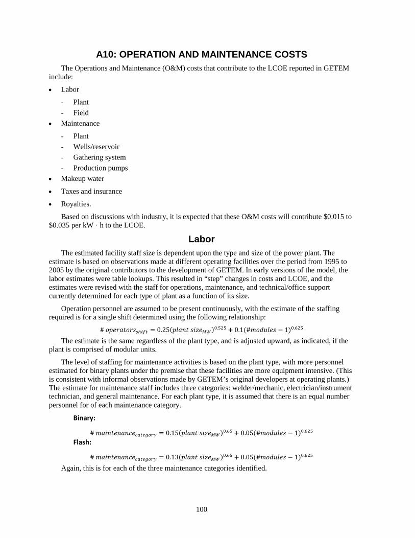
100

A10: OPERATION AND MAINTENANCE COSTS The Operations and Maintenance (O&M) costs that contribute to the LCOE reported in GETEM

include:

• Labor

- Plant - Field

• Maintenance

- Plant - Wells/reservoir - Gathering system - Production pumps

• Makeup water

• Taxes and insurance

• Royalties.

Based on discussions with industry, it is expected that these O&M costs will contribute $0.015 to $0.035 per kW · h to the LCOE.

Labor The estimated facility staff size is dependent upon the type and size of the power plant. The

estimate is based on observations made at different operating facilities over the period from 1995 to 2005 by the original contributors to the development of GETEM. In early versions of the model, the labor estimates were table lookups. This resulted in “step” changes in costs and LCOE, and the estimates were revised with the staff for operations, maintenance, and technical/office support currently determined for each type of plant as a function of its size.

Operation personnel are assumed to be present continuously, with the estimate of the staffing required is for a single shift determined using the following relationship:

# 𝑃𝑃𝑃𝑃𝑃𝑃𝑃𝑃𝑆𝑆𝑃𝑃𝑃𝑃𝑃𝑃𝑆𝑆𝑑𝑑ℎ𝑓𝑓𝑓𝑓𝑛𝑛 = 0.25(𝑃𝑃𝑆𝑆𝑆𝑆𝑃𝑃𝑃𝑃 𝑆𝑆𝑃𝑃𝑙𝑙𝑃𝑃𝑀𝑀𝑘𝑘)0.525 + 0.1(#𝑃𝑃𝑃𝑃𝑑𝑑𝑃𝑃𝑆𝑆𝑃𝑃𝑆𝑆 − 1)0.625

The estimate is the same regardless of the plant type, and is adjusted upward, as indicated, if the plant is comprised of modular units.

The level of staffing for maintenance activities is based on the plant type, with more personnel estimated for binary plants under the premise that these facilities are more equipment intensive. (This is consistent with informal observations made by GETEM’s original developers at operating plants.) The estimate for maintenance staff includes three categories: welder/mechanic, electrician/instrument technician, and general maintenance. For each plant type, it is assumed that there is an equal number personnel for of each maintenance category.

Binary:

# 𝑃𝑃𝑆𝑆𝑃𝑃𝑃𝑃𝑃𝑃𝑃𝑃𝑃𝑃𝑆𝑆𝑃𝑃𝑃𝑃𝑃𝑃𝑎𝑎𝑝𝑝𝑛𝑛𝑛𝑛𝑔𝑔𝑔𝑔𝑝𝑝𝑎𝑎 = 0.15(𝑃𝑃𝑆𝑆𝑆𝑆𝑃𝑃𝑃𝑃 𝑆𝑆𝑃𝑃𝑙𝑙𝑃𝑃𝑀𝑀𝑘𝑘)0.65 + 0.05(#𝑃𝑃𝑃𝑃𝑑𝑑𝑃𝑃𝑆𝑆𝑃𝑃𝑆𝑆 − 1)0.625 Flash:

# 𝑃𝑃𝑆𝑆𝑃𝑃𝑃𝑃𝑃𝑃𝑃𝑃𝑃𝑃𝑆𝑆𝑃𝑃𝑃𝑃𝑃𝑃𝑎𝑎𝑝𝑝𝑛𝑛𝑛𝑛𝑔𝑔𝑔𝑔𝑝𝑝𝑎𝑎 = 0.13(𝑃𝑃𝑆𝑆𝑆𝑆𝑃𝑃𝑃𝑃 𝑆𝑆𝑃𝑃𝑙𝑙𝑃𝑃𝑀𝑀𝑘𝑘)0.65 + 0.05(#𝑃𝑃𝑃𝑃𝑑𝑑𝑃𝑃𝑆𝑆𝑃𝑃𝑆𝑆 − 1)0.625

Again, this is for each of the three maintenance categories identified.

101

The staffing for technical support is the same for both plant types. It is a function only of the plant size. This support includes three categories: facility manager/engineer, operations management, and clerical/office. It is assumed that the level of support is equal for each of these three categories.

# 𝑃𝑃𝑃𝑃𝑃𝑃ℎ𝑃𝑃𝑃𝑃𝑃𝑃𝑆𝑆𝑆𝑆 𝑆𝑆𝑃𝑃𝑃𝑃𝑃𝑃𝑃𝑃𝑃𝑃𝑃𝑃𝑎𝑎𝑝𝑝𝑛𝑛𝑛𝑛𝑔𝑔𝑔𝑔𝑝𝑝𝑎𝑎 = 0.075(𝑃𝑃𝑆𝑆𝑆𝑆𝑃𝑃𝑃𝑃 𝑆𝑆𝑃𝑃𝑙𝑙𝑃𝑃𝑀𝑀𝑘𝑘)0.65

The annual man-hours for operations personnel is the product of number of operators per shift and the total hours in a year (8,760). The annual hours for each of the categories for both maintenance activities and technical support is the product of the number of staff for each category and an assumed 2,000 hrs for a year.

A direct labor rate is assumed for operators and each category for both maintenance and technical support. These values were defined in 2004, and are adjusted to the year for which the LCOE estimate is made using a producer price index for labor. A multiplier of 1.8 is applied to the labor cost to include indirect costs for benefits, overhead, home office, and similar costs. The rates used are summarized in Table A-6 below.

Table A-6. Hourly rates used to determine labor costs.

Staff Direct Labor Rate

(2004 Dollars) Operator $20/hr Welder/Mechanic $24/hr Electrician $24/hr General Maintenance $17.50/hr Facility Manager/Engineer $40/hr Operations Manager $30/hr Office/Clerical $12/hr

The labor rates and categories for O&M staffing are subjective. It is probable that operating

plants will have varying blends of staff capabilities, with some of the staff providing support in several areas. These estimates attempt to be representative of a typical staff composition.

GETEM does not provide an option to change the labor rates, the labor multiplier, or the type of personnel used; rather, the number of staff can be adjusted to revise the total labor cost.

In using the discounted cash flow method to determine the LCOE, the contribution of the O&M labor to the LCOE is reported as a single value. When the fixed charge rate method is used, a portion of the labor costs (25% of the operations labor) is attributed to the well field. The remaining labor costs are provided in the plant O&M contribution to the LCOE.

Maintenance Power Plant

The annual maintenance costs for the power plant are determined as a fraction of the total capital cost for the power plant. That default input for this value is 1.8% of the capital cost. The default is the same for both flash and binary plants.

Because the flash plants are assumed to utilize evaporative cooling systems, they are assumed to have an O&M cost associated with the treatment of the cooling water. There has been little information available upon which to estimate these costs. They are determined in GETEM using an approach based on information in a report prepared by Tetra Tech in 2008 that examined the modification of power plants in California from using cooling systems to using cooling towers. This

102

document indicated that costs for fouling and corrosion control would be $1.40 to $2.03 per gpm of cooling water flow (Table 5-2 from this document); a midpoint cost of $1.70/gpm is used as the default input (in 2007 dollars). This is the default used with GETEM’s estimate of cooling water flow rate to determine an annual chemical cost for the power plant.

𝑆𝑆𝑃𝑃𝑃𝑃𝑃𝑃𝑆𝑆𝑆𝑆 𝑃𝑃𝑆𝑆𝑆𝑆𝑃𝑃𝑃𝑃 𝑃𝑃ℎ𝑃𝑃𝑃𝑃𝑃𝑃𝑃𝑃𝑆𝑆𝑆𝑆 𝑃𝑃𝑃𝑃𝑆𝑆𝑃𝑃𝑆𝑆 = 𝑃𝑃𝑃𝑃𝑃𝑃𝑆𝑆𝑃𝑃𝑃𝑃𝑃𝑃 𝑃𝑃𝑆𝑆𝑃𝑃𝑃𝑃𝑃𝑃 𝑓𝑓𝑆𝑆𝑃𝑃𝑃𝑃 (𝑃𝑃𝑃𝑃𝑃𝑃) × 𝑃𝑃𝑃𝑃𝑃𝑃𝑆𝑆𝑃𝑃𝑃𝑃𝑃𝑃𝑃𝑃𝑃𝑃 𝑃𝑃𝑃𝑃𝑆𝑆𝑃𝑃 ($

𝑃𝑃𝑃𝑃𝑃𝑃)

A PPI for industrial chemicals is applied to bring costs to the year for which the LCOE is being estimated.

This is a recent change to GETEM, replacing previous placeholders for this cost. The values estimated with this methodology are lower than those previously estimated. This treatment cost is inherent to GETEM’s calculation and cannot be revised by anyone other than GTO.

Well Field and Gathering System The annual maintenance costs for the wells and surface piping are also determined as a fraction of

the capital cost for the well field and gathering system, including any well stimulation that is done. Only the costs of wells supporting the operation of the plant are used; costs of failed wells are not included unless used to supplement injection. The default for this inputted value is 1.5% of the capital cost, with the same default used for both flash and binary plants. These costs are for maintaining the surface equipment and injection pumps, and for work done on the wells and reservoir to maintain productivity. It does not include any makeup well drilling.

Because binary plants are assumed to have production pumps and to operate with minimum temperature constraints to prevent mineral precipitation, there are no brine chemical treatment costs included in the O&M costs for these plants. For flash plants, a treatment cost is included. There is minimal information available to estimate this cost, in part because of the variability in geothermal fluid chemistries. GETEM’s default for this cost is taken from Gallup’s 2005 Geothermics paper. The mean values to treat 1,000 tonnes of brine is $22.50 (Table 2 in this paper), in 2005 dollars. GETEM’s estimate of the flow required to produce a specified level of sales is used with this value to determine the default annual brine treatment cost.

𝑆𝑆𝑃𝑃𝑃𝑃𝑃𝑃𝑆𝑆𝑆𝑆 𝑏𝑏𝑃𝑃𝑃𝑃𝑃𝑃𝑃𝑃 𝑃𝑃ℎ𝑃𝑃𝑃𝑃𝑃𝑃𝑃𝑃𝑆𝑆𝑆𝑆 𝑃𝑃𝑃𝑃𝑆𝑆𝑃𝑃𝑆𝑆

= 𝑆𝑆𝑃𝑃𝑃𝑃𝑃𝑃𝑆𝑆𝑆𝑆 𝑃𝑃𝑃𝑃𝑃𝑃𝑃𝑃ℎ𝑃𝑃𝑃𝑃𝑃𝑃𝑆𝑆𝑆𝑆 𝑓𝑓𝑆𝑆𝑃𝑃𝑃𝑃 �𝑘𝑘𝑃𝑃𝑐𝑐𝑃𝑃� × 𝑃𝑃ℎ𝑃𝑃𝑃𝑃𝑃𝑃𝑃𝑃𝑆𝑆𝑆𝑆 𝑃𝑃𝑃𝑃𝑆𝑆𝑃𝑃(

$1,000 𝑃𝑃𝑃𝑃𝑃𝑃𝑃𝑃𝑃𝑃𝑆𝑆 𝑃𝑃𝑓𝑓 𝑃𝑃𝑃𝑃𝑃𝑃𝑃𝑃ℎ𝑃𝑃𝑃𝑃𝑃𝑃𝑆𝑆𝑆𝑆 𝑓𝑓𝑆𝑆𝑃𝑃𝑃𝑃𝑑𝑑)

This cost is adjusted to the year for which GETEM is estimating the LCOE using a PPI for industrial chemicals.

This is also a recent change, replacing the previous placeholders used to estimate this cost. The resulting annual cost is higher than obtained with the placeholders. This is not a GETEM default input that can be revised. If it needs to be changed, the maintenance cost multiplier for the well field can be used to adjust the total O&M cost for the well field.

Production Pumps The costs to maintain the production pumps is not included in the maintenance cost determined

for the well field and surface equipment. These pumps are periodically replaced or taken out of service and re-built. The default is the use of a line-shaft pump, which is assumed to have a longer operating life (3 years) than an electric submersible pump (2 years). At the end of the life, the pump is removed and replaced. There is no additional cost for the pump casing, but there are time and cost requirements for the removal and installation of the new pump.

𝑃𝑃𝑃𝑃𝑃𝑃𝑃𝑃 𝑃𝑃𝑃𝑃𝑆𝑆𝑃𝑃𝑝𝑝𝑛𝑛𝑝𝑝𝑓𝑓𝑝𝑝𝑎𝑎𝑛𝑛𝑝𝑝𝑛𝑛𝑛𝑛𝑛𝑛 = 𝑃𝑃𝑃𝑃𝑃𝑃𝑃𝑃 𝑃𝑃𝑃𝑃𝑆𝑆𝑃𝑃 + 𝑃𝑃𝑃𝑃𝑆𝑆𝑃𝑃𝑆𝑆𝑆𝑆𝑆𝑆𝑆𝑆𝑃𝑃𝑃𝑃𝑃𝑃𝑃𝑃 𝑃𝑃𝑃𝑃𝑆𝑆𝑃𝑃𝑝𝑝𝑛𝑛𝑝𝑝 𝑓𝑓𝑛𝑛�𝑑𝑑𝑃𝑃𝑃𝑃𝑃𝑃ℎ𝑑𝑑𝑛𝑛𝑛𝑛𝑛𝑛𝑓𝑓𝑛𝑛𝑔𝑔� + 𝑃𝑃𝑃𝑃𝑃𝑃𝑘𝑘𝑃𝑃𝑙𝑙𝑃𝑃𝑃𝑃 𝑃𝑃𝑃𝑃𝑃𝑃 𝑓𝑓𝑃𝑃𝑃𝑃 1 𝑑𝑑𝑆𝑆𝑐𝑐

103

There is no built-in schedule for pump replacement. Instead, it is assumed that a fraction of total pumps in service will be replaced each year as indicated in the relationship below for the annual maintenance costs.

𝑆𝑆𝑃𝑃𝑃𝑃𝑃𝑃𝑆𝑆𝑆𝑆 𝑃𝑃𝑃𝑃𝑃𝑃𝑃𝑃 𝑃𝑃𝑃𝑃𝑆𝑆𝑃𝑃𝑝𝑝𝑛𝑛𝑝𝑝𝑓𝑓𝑝𝑝𝑎𝑎𝑛𝑛𝑝𝑝𝑛𝑛𝑛𝑛𝑛𝑛 = 𝑃𝑃𝑃𝑃𝑃𝑃𝑃𝑃 𝑃𝑃𝑃𝑃𝑆𝑆𝑃𝑃𝑝𝑝𝑛𝑛𝑝𝑝𝑓𝑓𝑝𝑝𝑎𝑎𝑛𝑛𝑝𝑝𝑛𝑛𝑛𝑛𝑛𝑛 �#𝑃𝑃𝑃𝑃𝑃𝑃𝑃𝑃𝑆𝑆 𝑃𝑃𝑃𝑃 𝑆𝑆𝑃𝑃𝑃𝑃𝑙𝑙𝑃𝑃𝑃𝑃𝑃𝑃𝑃𝑃𝑃𝑃𝑃𝑃𝑃𝑃 𝑆𝑆𝑃𝑃𝑓𝑓𝑃𝑃 𝑃𝑃𝑃𝑃 𝑐𝑐𝑃𝑃𝑆𝑆

�

Line-shaft pumps will have an annual cost for the lubricant used for the shaft bearings. The placeholder values previously used to determine this cost have been revised. Little information has been published on the amount of oil needed to lubricate a pump. The placeholders related the consumption of oil to the brine flow rate. It is more probable that the consumption will be related to the pump setting depth. A GRC paper (Price and Burleigh 2001) provides a cost of $4,300 annually for a pump with a setting depth of 500 ft. This information was incorporated into the following relationship to estimate the annual oil cost per line-shaft production pump:

𝑆𝑆𝑃𝑃𝑃𝑃𝑃𝑃𝑆𝑆𝑆𝑆 𝑃𝑃𝑃𝑃𝑆𝑆𝑃𝑃𝑔𝑔𝑓𝑓𝑓𝑓 = 𝑆𝑆𝐶𝐶 × 𝑆𝑆𝑃𝑃𝑃𝑃𝑃𝑃𝑆𝑆𝑆𝑆 𝑃𝑃𝑃𝑃𝑆𝑆𝑃𝑃𝑝𝑝𝑛𝑛𝑓𝑓𝑛𝑛𝑝𝑝𝑛𝑛𝑛𝑛𝑎𝑎𝑛𝑛−𝑔𝑔𝑓𝑓𝑓𝑓 if pump setting depth =0, SF = 0

if pump setting depth <250 ft, SF = 0.5

if pump setting depth >250 ft, SF = pump setting depth/reference depth.

In these relationships, the reference setting depth is 500 ft and the reference annual cost is $4,300 (both values from Price’s paper). It is probable that some minimum amount of oil will be required regardless of the depth, and, though it is somewhat arbitrary, setting the scaling factor (SF) to 0.5 for depths less than 250 ft captures this minimum requirement. The reference annual oil cost of $4,300 per pump is in 2001 dollars. That value is adjusted using the PPI for refined petroleum products. These costs and reference depth are not default values that can be revised.

Makeup Water Discussion on the determination of the amount of water that must be made up annually is

provided in both Appendix A9 and Appendix A11. Costs for water are dependent upon both location and the quality of the water required. A report from Sandia National Laboratory (Tidwell 2013) used a cost of $0.35 per kW · h, which is the energy cost to lift, move, and treat water. If the makeup water has to be lifted 250 ft, then the energy cost for 1 acre-ft of water would be ~$146. In the western states (exclusive of California), the cost for appropriated and unappropriated ground water ranges from $16 to $250 per acre-ft. This cost and the energy cost to deliver the water are the basis of GETEM’s default of $300 per acre ft for makeup water for hydrothermal flash and EGS binary plants.

It is postulated that, when using flash plants with EGS resources, a higher-quality makeup water will be required. This is based on the premise that if flashed steam condensate is used as makeup for heat rejection, a similar-quality water will be needed to replace this fluid. If not, it is possible that the concentration of dissolved solids in fluid circulating through the EGS reservoir will increase with time, leading to potential operational problems both in the surface facilities and the subsurface reservoir. The Sandia report indicates that the cost of using brackish groundwater is in the range of $1,500 to $2,000+ per acre ft. This cost includes well drilling and RO treatment to provide the desired water quality. This is the basis for GETEM’s default of $2,000 per acre-ft for makeup water for EGS flash plant scenarios. There are no PPIs applied to water costs.

104

Taxes and Insurance Taxes refer to property taxes, not sales taxes on revenue. The annual taxes and insurance costs are

determined as a specified fraction or percentage of capital costs. The capital costs used are the plant cost and the cost of the wells and surface equipment that support plant operation. (Any stimulation costs associated with the wells are also included). Costs of failed wells, or costs at sites not developed, are not included.

The default for this annual tax and insurance rate is 0.75%. This value is based on the industry interviews by GTO’s LCOE analysis team.

Royalties GETEM assumes that royalties are paid per the BLM royalty schedule, in which the royalty

payments for the first 10 years of operation are 1.75% of revenues. After 10 years, royalties are 3.5% of revenues.

This rate schedule was taken from 2007 Federal Register 43 CFR, Part 3200.

105

A11: POWER PLANT Different methodologies are used in estimating the costs and performance of air-cooled binary

and flash steam power plants. The ability to select different working fluids and varying process conditions within the binary cycle provides an additional degree of freedom in designing air-cooled binary plants. This added degree of design flexibility requires an alternative approach in GETEM when determining plant cost and performance of projects using air-cooled binary plants.

The following discussions provide detail as to how plant performance and cost are determined for both types of power plants.

Flash Steam Plants Flash Conditions

Either single-flash or dual-flash power plants can be evaluated. While there has been a recent installation of a triple-flash plant, that configuration is not a current option in GETEM. Unlike the air-cooled binary plants, which are characterized in GETEM based on a fixed ambient temperature of 10°C, a design wet bulb (heat sink) temperature can be specified for the flash plant. Inherent to the flash plant calculations are default inputs for the cooling water temperature rise and approach temperatures in both the cooling tower and the condenser. The values used are representative of a limited number of plants for which information was available; they are default inputs that cannot be revised. The default values for the approach temperatures and cooling water temperature rise are used with the specified wet bulb temperature to determine a condensing temperature. The condensing temperature and the specified resource temperature are used in an approach described by DiPippo (2012) to find near optimal flash-separator temperatures. DiPippo refers to this approach as the “equal-temperature-split” rule, in which the temperature range between the resource temperature and condenser is divided into equal segments. The number of segments is equivalent to the number of flash plus one. These flash temperatures (defined below) represent the final temperature (and pressure) in the flashing process, in which the steam vapor is separated from the unflashed liquid.

𝑇𝑇𝑑𝑑𝑓𝑓𝑛𝑛𝑔𝑔𝑓𝑓𝑛𝑛 𝑓𝑓𝑓𝑓𝑝𝑝𝑑𝑑ℎ =(𝑇𝑇𝑝𝑝𝑛𝑛𝑑𝑑𝑔𝑔𝑓𝑓𝑝𝑝𝑎𝑎𝑛𝑛 − 𝑇𝑇𝑎𝑎𝑔𝑔𝑛𝑛𝑓𝑓𝑛𝑛𝑛𝑛𝑑𝑑𝑛𝑛𝑝𝑝)

2

𝑇𝑇𝐻𝐻𝑃𝑃−𝑓𝑓𝑓𝑓𝑝𝑝𝑓𝑓 𝑓𝑓𝑓𝑓𝑝𝑝𝑑𝑑ℎ = 𝑇𝑇𝑝𝑝𝑛𝑛𝑑𝑑𝑔𝑔𝑓𝑓𝑝𝑝𝑎𝑎𝑛𝑛 −(𝑇𝑇𝑝𝑝𝑛𝑛𝑑𝑑𝑔𝑔𝑓𝑓𝑝𝑝𝑎𝑎𝑛𝑛 − 𝑇𝑇𝑎𝑎𝑔𝑔𝑛𝑛𝑓𝑓𝑛𝑛𝑛𝑛𝑑𝑑𝑛𝑛𝑝𝑝)

3

𝑇𝑇𝐿𝐿𝑃𝑃−𝑓𝑓𝑓𝑓𝑝𝑝𝑓𝑓 𝑓𝑓𝑓𝑓𝑝𝑝𝑑𝑑ℎ = 𝑇𝑇𝑝𝑝𝑛𝑛𝑑𝑑𝑔𝑔𝑓𝑓𝑝𝑝𝑎𝑎𝑛𝑛 − 2 ×(𝑇𝑇𝑝𝑝𝑛𝑛𝑑𝑑𝑔𝑔𝑓𝑓𝑝𝑝𝑎𝑎𝑛𝑛 − 𝑇𝑇𝑎𝑎𝑔𝑔𝑛𝑛𝑓𝑓𝑛𝑛𝑛𝑛𝑑𝑑𝑛𝑛𝑝𝑝)

3

In these relationships, HP refers to the higher-pressure flash and LP to the lower-pressure flash. The condenser temperature is determined as:

𝑇𝑇𝑎𝑎𝑔𝑔𝑛𝑛𝑓𝑓𝑛𝑛𝑛𝑛𝑑𝑑𝑛𝑛𝑝𝑝 = 𝑇𝑇𝑤𝑤𝑛𝑛𝑛𝑛 𝑏𝑏𝑓𝑓𝑓𝑓𝑏𝑏 + ∆𝑇𝑇𝑎𝑎𝑔𝑔𝑔𝑔𝑓𝑓𝑓𝑓𝑛𝑛𝑔𝑔 𝑛𝑛𝑔𝑔𝑤𝑤𝑛𝑛𝑝𝑝 𝑝𝑝𝑝𝑝𝑝𝑝𝑝𝑝𝑔𝑔𝑝𝑝𝑎𝑎ℎ + ∆𝑇𝑇𝑎𝑎𝑔𝑔𝑔𝑔𝑓𝑓𝑓𝑓𝑛𝑛𝑔𝑔 𝑤𝑤𝑝𝑝𝑛𝑛𝑛𝑛𝑝𝑝 + ∆𝑇𝑇𝑎𝑎𝑔𝑔𝑛𝑛𝑓𝑓𝑛𝑛𝑛𝑛𝑑𝑑𝑛𝑛𝑝𝑝 𝑝𝑝𝑝𝑝𝑝𝑝𝑝𝑝𝑔𝑔𝑝𝑝𝑎𝑎ℎ

The flash temperatures determined represent the near optimal turbine inlet condition (saturated vapor at these temperatures). In the operation of a flash plant, constraints may be imposed that preclude operation at these conditions. One constraint on operation is that the steam pressures upstream of the turbine be greater than one atmosphere to prevent air leakage into the steam. (This leakage would add to the non-condensable gases that must be removed from the condenser.) This constraint is more likely to occur with dual-flash plants (which are the GETEM default). Using the approach described, this limit would be reached for the low-pressure flash at resource temperatures less than 230°C, assuming a condenser temperature of 35°C; with a 40°C condensing temperature, the limit would be reached for resource temperatures less than 220°C.

Another constraint placed on temperature would be to prevent mineral precipitation; in GETEM, a constraint is imposed to prevent precipitation of amorphous silica.

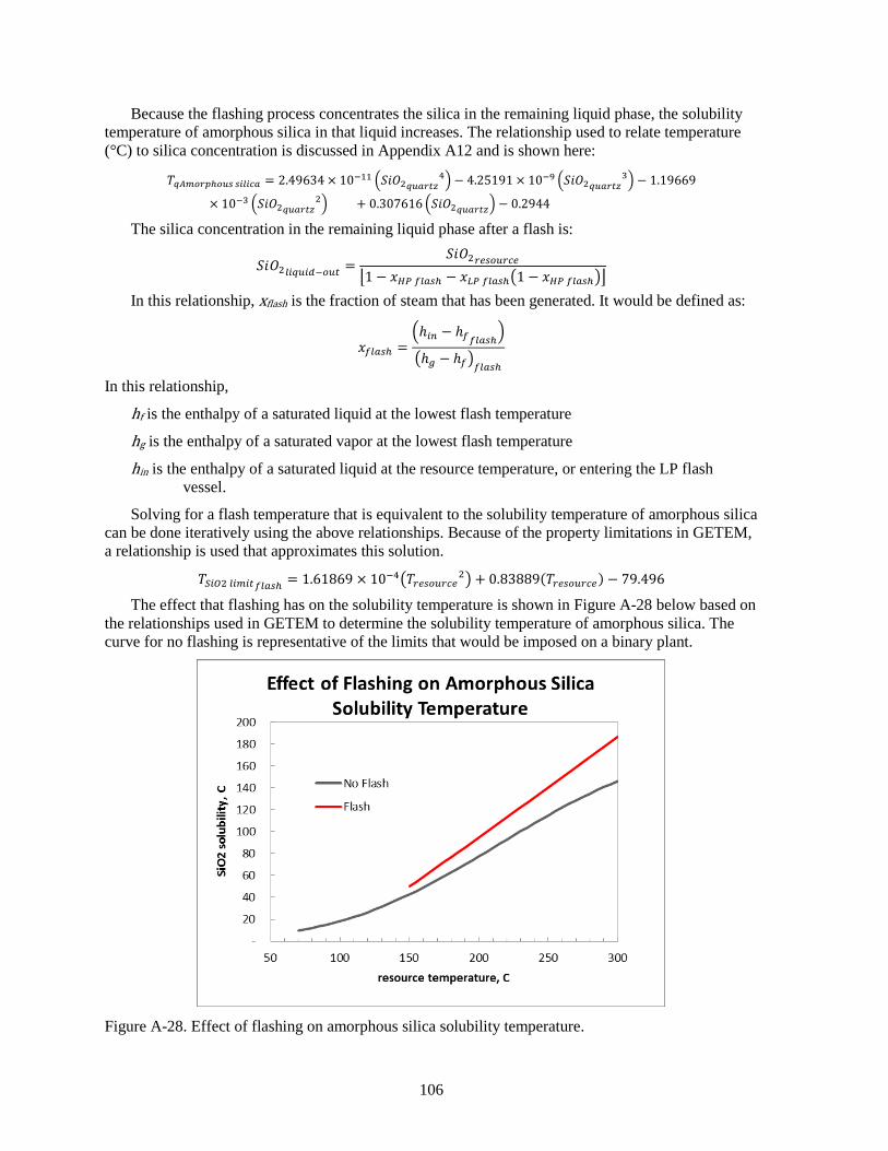
106

Because the flashing process concentrates the silica in the remaining liquid phase, the solubility temperature of amorphous silica in that liquid increases. The relationship used to relate temperature (°C) to silica concentration is discussed in Appendix A12 and is shown here:

𝑇𝑇𝑟𝑟𝑃𝑃𝑝𝑝𝑔𝑔𝑝𝑝𝑝𝑝ℎ𝑔𝑔𝑓𝑓𝑑𝑑 𝑑𝑑𝑓𝑓𝑓𝑓𝑓𝑓𝑎𝑎𝑝𝑝 = 2.49634 × 10−11 �𝑆𝑆𝑃𝑃𝑂𝑂2𝑟𝑟𝑓𝑓𝑝𝑝𝑝𝑝𝑛𝑛𝑞𝑞4� − 4.25191 × 10−9 �𝑆𝑆𝑃𝑃𝑂𝑂2𝑟𝑟𝑓𝑓𝑝𝑝𝑝𝑝𝑛𝑛𝑞𝑞

3� − 1.19669

× 10−3 �𝑆𝑆𝑃𝑃𝑂𝑂2𝑟𝑟𝑓𝑓𝑝𝑝𝑝𝑝𝑛𝑛𝑞𝑞2� + 0.307616 �𝑆𝑆𝑃𝑃𝑂𝑂2𝑟𝑟𝑓𝑓𝑝𝑝𝑝𝑝𝑛𝑛𝑞𝑞� − 0.2944

The silica concentration in the remaining liquid phase after a flash is:

𝑆𝑆𝑃𝑃𝑂𝑂2𝑓𝑓𝑓𝑓𝑟𝑟𝑓𝑓𝑓𝑓𝑓𝑓−𝑔𝑔𝑓𝑓𝑛𝑛 =𝑆𝑆𝑃𝑃𝑂𝑂2𝑝𝑝𝑛𝑛𝑑𝑑𝑔𝑔𝑓𝑓𝑝𝑝𝑎𝑎𝑛𝑛

�1 − 𝐼𝐼𝐻𝐻𝑃𝑃 𝑓𝑓𝑓𝑓𝑝𝑝𝑑𝑑ℎ − 𝐼𝐼𝐿𝐿𝑃𝑃 𝑓𝑓𝑓𝑓𝑝𝑝𝑑𝑑ℎ�1 − 𝐼𝐼𝐻𝐻𝑃𝑃 𝑓𝑓𝑓𝑓𝑝𝑝𝑑𝑑ℎ��

In this relationship, xflash is the fraction of steam that has been generated. It would be defined as:

𝐼𝐼𝑓𝑓𝑓𝑓𝑝𝑝𝑑𝑑ℎ =�ℎ𝑓𝑓𝑛𝑛 − ℎ𝑓𝑓𝑓𝑓𝑓𝑓𝑝𝑝𝑑𝑑ℎ�

�ℎ𝑔𝑔 − ℎ𝑓𝑓�𝑓𝑓𝑓𝑓𝑝𝑝𝑑𝑑ℎ

In this relationship,

hf is the enthalpy of a saturated liquid at the lowest flash temperature

hg is the enthalpy of a saturated vapor at the lowest flash temperature

hin is the enthalpy of a saturated liquid at the resource temperature, or entering the LP flash vessel.

Solving for a flash temperature that is equivalent to the solubility temperature of amorphous silica can be done iteratively using the above relationships. Because of the property limitations in GETEM, a relationship is used that approximates this solution.

𝑇𝑇𝑆𝑆𝑓𝑓𝑂𝑂2 𝑓𝑓𝑓𝑓𝑝𝑝𝑓𝑓𝑛𝑛𝑓𝑓𝑓𝑓𝑝𝑝𝑑𝑑ℎ = 1.61869 × 10−4�𝑇𝑇𝑝𝑝𝑛𝑛𝑑𝑑𝑔𝑔𝑓𝑓𝑝𝑝𝑎𝑎𝑛𝑛2� + 0.83889(𝑇𝑇𝑝𝑝𝑛𝑛𝑑𝑑𝑔𝑔𝑓𝑓𝑝𝑝𝑎𝑎𝑛𝑛) − 79.496

The effect that flashing has on the solubility temperature is shown in Figure A-28 below based on the relationships used in GETEM to determine the solubility temperature of amorphous silica. The curve for no flashing is representative of the limits that would be imposed on a binary plant.

Figure A-28. Effect of flashing on amorphous silica solubility temperature.

107

In establishing the flash temperatures used, the optimal flash temperature for the low-pressure flash (or the single-flash temperature) is compared to the temperature constraints imposed by a 1 atm minimum flash pressure and the amorphous silica solubility temperature determined for the unflashed brine. The highest of these temperatures is used as the flash temperature. The temperature for the high-pressure flash is halfway between this temperature and the temperature of the geothermal resource.

Note that it is assumed that the production wells that supply the flash plant are not pumped. If the estimated wellhead pressure is less than the flash pressure determined, a warning occurs. Regardless of the warning, the flash pressure determined by the approach described above is used to determine the plant performance and cost.

In an operating plant, there will be a frictional pressure drop between the separator vessel and the turbine. The optimal temperatures and a default pressure drop are used to determine the flash-separator pressures.

𝑃𝑃1𝑑𝑑𝑛𝑛 𝑓𝑓𝑓𝑓𝑝𝑝𝑑𝑑ℎ = 𝑃𝑃𝑑𝑑𝑝𝑝𝑛𝑛𝑓𝑓𝑝𝑝𝑝𝑝𝑛𝑛𝑓𝑓𝑔𝑔𝑛𝑛@𝑇𝑇1𝑠𝑠𝑠𝑠 𝑒𝑒𝑖𝑖𝑠𝑠𝑠𝑠ℎ 𝑜𝑜𝑝𝑝𝑠𝑠𝑖𝑖𝑡𝑡𝑜𝑜𝑡𝑡+ ∆𝑃𝑃𝑓𝑓𝑝𝑝𝑓𝑓𝑎𝑎𝑛𝑛𝑓𝑓𝑔𝑔𝑛𝑛

𝑃𝑃2𝑛𝑛𝑓𝑓 𝑓𝑓𝑓𝑓𝑝𝑝𝑑𝑑ℎ = 𝑃𝑃𝑑𝑑𝑝𝑝𝑛𝑛𝑓𝑓𝑝𝑝𝑝𝑝𝑛𝑛𝑓𝑓𝑔𝑔𝑛𝑛@𝑇𝑇2𝑖𝑖𝑛𝑛 𝑒𝑒𝑖𝑖𝑠𝑠𝑠𝑠ℎ 𝑜𝑜𝑝𝑝𝑠𝑠𝑖𝑖𝑡𝑡𝑜𝑜𝑡𝑡+ ∆𝑃𝑃𝑓𝑓𝑝𝑝𝑓𝑓𝑎𝑎𝑛𝑛𝑓𝑓𝑔𝑔𝑛𝑛

In these relationships, P1st flash is the pressure in a single-flash plant, or in a dual-flash plant, it is the higher flash pressure. P2nd flash is the lower pressure in a dual-flash plant. The default pressure drop is 1 psi; this is not a model input that can be revised.

Steam Flow With the determination of the flash-separator pressures, the fraction of steam produced by each

flash can be determined.

𝐼𝐼1𝑑𝑑𝑛𝑛 𝑓𝑓𝑓𝑓𝑝𝑝𝑑𝑑ℎ =�ℎ𝑝𝑝𝑛𝑛𝑑𝑑𝑔𝑔𝑓𝑓𝑝𝑝𝑎𝑎𝑛𝑛 − ℎ𝑓𝑓@𝑃𝑃1𝑠𝑠𝑠𝑠 𝑒𝑒𝑖𝑖𝑠𝑠𝑠𝑠ℎ

�

�ℎ𝑔𝑔 − ℎ𝑓𝑓�@𝑃𝑃1𝑠𝑠𝑠𝑠 𝑒𝑒𝑖𝑖𝑠𝑠𝑠𝑠ℎ

𝐼𝐼2𝑛𝑛𝑓𝑓 𝑓𝑓𝑓𝑓𝑝𝑝𝑑𝑑ℎ =�ℎ𝑓𝑓@𝑃𝑃1𝑠𝑠𝑠𝑠 𝑒𝑒𝑖𝑖𝑠𝑠𝑠𝑠ℎ

− ℎ𝑓𝑓@𝑃𝑃2𝑖𝑖𝑛𝑛 𝑒𝑒𝑖𝑖𝑠𝑠𝑠𝑠ℎ�

�ℎ𝑔𝑔 − ℎ𝑓𝑓�@𝑃𝑃2𝑖𝑖𝑛𝑛 𝑒𝑒𝑖𝑖𝑠𝑠𝑠𝑠ℎ

where

hf is the enthalpy of a saturated liquid at the indicated pressure

hg is the enthalpy of a saturated vapor at the indicated pressure

hresource is the enthalpy of a saturated liquid at the resource temperature.

The steam flow from each flash is determined as:

��𝑃𝑑𝑑𝑛𝑛𝑛𝑛𝑝𝑝𝑝𝑝1𝑠𝑠𝑠𝑠 𝑒𝑒𝑖𝑖𝑠𝑠𝑠𝑠ℎ = 𝐼𝐼1𝑑𝑑𝑛𝑛 𝑓𝑓𝑓𝑓𝑝𝑝𝑑𝑑ℎ���𝑃𝑔𝑔𝑓𝑓−𝑓𝑓𝑛𝑛� ��𝑃𝑑𝑑𝑛𝑛𝑛𝑛𝑝𝑝𝑝𝑝2𝑖𝑖𝑛𝑛 𝑒𝑒𝑖𝑖𝑠𝑠𝑠𝑠ℎ = 𝐼𝐼2𝑛𝑛𝑓𝑓 𝑓𝑓𝑓𝑓𝑝𝑝𝑑𝑑ℎ(1 − 𝐼𝐼1𝑑𝑑𝑛𝑛 𝑓𝑓𝑓𝑓𝑝𝑝𝑑𝑑ℎ)���𝑃𝑔𝑔𝑓𝑓−𝑓𝑓𝑛𝑛�

The determination of plant performance in GETEM is based on a fixed geothermal flow (mgf-in) of 1,000 lb/hr into the plant. This flow rate is arbitrary, but allows the plant performance to be determined on a per-unit-mass basis. Once this performance metric is known, the specified power sales can be used to determine the total geothermal flow required and the equipment sized.

108

Non-Condensable Gas Removal During the flashing process, dissolved gases will come out of the solution and expand with the

steam through the turbine. While the work done in expanding these gases is not estimated, the work required to remove the gases from the condenser is estimated. The removal system in GETEM is a hybrid system, with the first two stages using steam ejectors and final 3rd stage using a vacuum pump.

The amount of non-condensable gases in the geothermal fluid is specified as a fraction (ppm by mass).

mncg = xncg�mgf−in� While all of the non-condensable gases are removed from the condenser, they are allowed to

accumulate in the plant’s main steam condenser until their partial pressure reaches a limit defined as:

Pncg = 0.0000825�xncg� + 0.15 , where

Pncg is the partial pressure of the gases in inches Hg, and

xncg is the gas concentration in ppm by mass.

This relationship is representative of information from a limited number of operating plants. The turbine exhaust pressure (and condenser pressure) used is the sum of the saturation pressure of water at the condenser temperature determined and the partial pressure of the non-condensable gases:

𝑃𝑃𝑛𝑛𝑓𝑓𝑝𝑝𝑏𝑏𝑓𝑓𝑛𝑛𝑛𝑛 𝑛𝑛𝑒𝑒ℎ𝑝𝑝𝑓𝑓𝑑𝑑𝑛𝑛 = 𝑃𝑃𝑎𝑎𝑔𝑔𝑛𝑛𝑓𝑓𝑛𝑛𝑛𝑛𝑑𝑑𝑛𝑛𝑝𝑝 = 𝑃𝑃𝑑𝑑𝑝𝑝𝑛𝑛𝑓𝑓𝑝𝑝𝑝𝑝𝑛𝑛𝑓𝑓𝑔𝑔𝑛𝑛 @ 𝑇𝑇,𝑎𝑎𝑔𝑔𝑛𝑛𝑓𝑓𝑛𝑛𝑛𝑛𝑑𝑑𝑛𝑛𝑝𝑝 + 𝑃𝑃𝑛𝑛𝑎𝑎𝑔𝑔 This partial pressure is also used to determine the amount of water vapor removed with the

non-condensable gases:

mwaterremoved = mncg �Psaturation @ T,condenser

Pncg� �

Mol WtwaterMol Wtncg

�

It is assumed that the molecular weight (Mol Wt) of the non-condensable gases is that of carbon dioxide (44 g per mole).

The amount of vapor removed from the condenser is the sum of the water vapor and the non-condensable gas, or:

mremoved = mncg �1 + �Psaturation @ T,condenser

Pncg� �

Mol WtwaterMol Wtncg

��

A three-stage removal system is inherent to the calculations. It is assumed that the pressure ratios across each stage are equivalent, where

pressure ratiostage =PdischargePsuction

= eln�1 atm

Pcondenser� �#stages

A condenser at the exhaust of each stage is used to recover steam condensate from the vent stream and reduce the flow to the subsequent stage; by reducing flow, the energy requirements for the next stage are reduced. The condensers for each stage operate at the same temperature as the main plant steam condenser, allowing the partial pressure of the non-condensable gases in a given stage condenser to be determined.

Pncgstage = pressure ratiostage × (Psuction) − Psaturation @ T,condenser

The Psuction term in this relationship is the discharge pressure from the previous stage, or for the first stage of the removal system, it is the condenser (turbine exhaust) pressure.

109

The partial pressure for a stage is used to determine the amount of vapor that is removed by the subsequent stage.

mremovednext stage = mncg �1 + �Psaturation @ T,condenser

Pncgstage� �

Mol WtwaterMol Wtncg

��

Because the non-condensable partial pressure increases in each successive stage, the amount of water vapor in the vent stream is reduced, as is the energy required for that stage.

The steam ejectors used for the first two stages utilize the highest-pressure steam available. The methods used to establish the steam required were adapted from the performances curves for single stage ejectors in Perry’s Chemical Engineer’s Handbook (Green). Correlations developed from these performance curves are used to determine the mass ratio between the suction gas (condenser vent stream) and the motive gas (steam from the highest-pressure separator). The basic methodology is given below.

- Determine pressure ratio of vent gas to the motive steam (PRm) through the following:

PRm =Psaturation @ T,condenser + Pncg

PHP flash

- Determine the optimum area ratio (AR) for the nozzle using this motive pressure ratio and the stage pressure ratio:

AR = �3.5879�pressure ratiostage−2.1168� + 1�PRm�−1.155�pressure ratiostage

−0.0453�� - Determine the uncorrected entrainment ratio (ERu) using this area ratio and the motive

pressure ratio:

ERu = PRm�2.9594�AR−0.8458+0.99�� × [1.0035(AR) + 8.9374]

- This entrainment ratio is corrected to account for temperature and molecular weight differences (temperatures are in absolute units, in °R). The molecular weight of the vent stream is based on the composition of the stream at the ejector suction:

entrainment ratio = ERu �Tsteam(Mol Wtvent stream)Tcondenser(Mol Wtwater) �

0.5

- From this entrainment ratio, the steam flow for the stage is determined:

steam flowstage =mremovedstage

entrainment ratio

This calculation is made for each ejector stage, with the motive pressure ratio decreasing with each successive stage. The total steam required is the sum of that steam required for the first and second stages of the removal system. All steam required for NCG removal is provided by the highest-pressure flash/separator.

For the last (third) stage, a vacuum pump is utilized. The vent flow rate is that leaving the second stage condenser. The head is determined based on the pressure difference between 1 atm and the second stage pressure, and a density that is based on the pressure, temperature, and molecular weight of the vent stream at the pump suction. The default vacuum pump efficiency (η) is 70%.

powervacuum pump =mvent stream�∆P3rd stage�ηvacuum pump(ρvent stream)

There is also a power requirement to bring the liquid condensate from each stage condenser to 1 atmosphere. For the first and second stage, the liquid condensate includes the motive steam for the ejector and a portion of the water vapor that enters the ejector with the non-condensable. The default efficiency used for these condensate pumps is 75%.

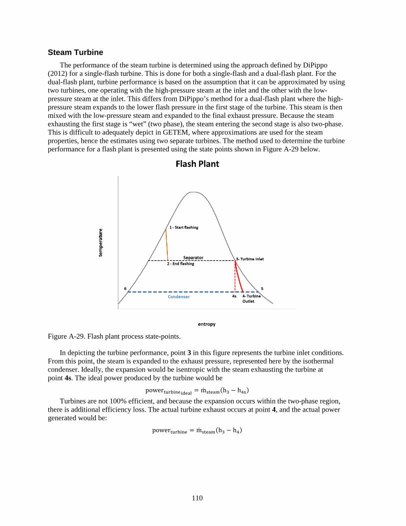
110

Steam Turbine The performance of the steam turbine is determined using the approach defined by DiPippo

(2012) for a single-flash turbine. This is done for both a single-flash and a dual-flash plant. For the dual-flash plant, turbine performance is based on the assumption that it can be approximated by using two turbines, one operating with the high-pressure steam at the inlet and the other with the low-pressure steam at the inlet. This differs from DiPippo’s method for a dual-flash plant where the high-pressure steam expands to the lower flash pressure in the first stage of the turbine. This steam is then mixed with the low-pressure steam and expanded to the final exhaust pressure. Because the steam exhausting the first stage is “wet” (two phase), the steam entering the second stage is also two-phase. This is difficult to adequately depict in GETEM, where approximations are used for the steam properties, hence the estimates using two separate turbines. The method used to determine the turbine performance for a flash plant is presented using the state points shown in Figure A-29 below.

Figure A-29. Flash plant process state-points.

In depicting the turbine performance, point 3 in this figure represents the turbine inlet conditions. From this point, the steam is expanded to the exhaust pressure, represented here by the isothermal condenser. Ideally, the expansion would be isentropic with the steam exhausting the turbine at point 4s. The ideal power produced by the turbine would be

powerturbineideal = msteam(h3 − h4s)

Turbines are not 100% efficient, and because the expansion occurs within the two-phase region, there is additional efficiency loss. The actual turbine exhaust occurs at point 4, and the actual power generated would be:

powerturbine = msteam(h3 − h4)

111

Using the approach given by DiPippo (2012), the enthalpy of the steam exhausting the turbine at point 4 can be determined as:

h4 =h3 − A �1 − h6

(h5 − h6)�

�1 + A(h5 − h6)�

where A is

A =ηturbine(h3 − h4s)

2

h6 is the saturation enthalpy of liquid water at the exhaust pressure

h5 is the saturation enthalpy of water vapor at the exhaust pressure

h3 is the turbine inlet enthalpy

h4s is the enthalpy with a constant entropy expansion to the exhaust pressure

ηturbine is the turbine efficiency (dry expansion) – GETEM default value is 80%.

As indicated, the turbine power is: powerturbine = msteam(h3 − h4)

The steam flow rate used for the higher-pressure turbine in a dual-flash plant, or the turbine in a single-flash plant, is the amount of steam generated during the flashing process less the portion of this higher-pressure steam used to operate the steam ejectors in the non-condensable gas removal system.

msteam = msteam1st flash −� Steam flowncg stage

With the dual-flash plants, the steam flow to the low-pressure turbine is equivalent to the amount of steam generated in the second or low-pressure flash.

The turbine power is determined for each turbine in a dual-flash system using the approach described. The total turbine output is the sum of the high- and low-pressure turbine outputs.

Heat Rejection The amount of heat that is rejected is the sum of the heat duty of the main steam condenser and

the heat duty of the condensers for each stage of the non-condensable gas removal system.

The heat duty (Q) for the main condenser is based on the enthalpy of the combined steam flow exiting the turbines, the total steam flow, and the saturated enthalpy of liquid water at the condensing temperature.

Qcondenser = [(mstmhturbine exhaust)HP + (mstmhturbine exhaust)LP] − �hf @Tcondenser�mstmHP + mstmLP��

In the non-condensable gas removal system, the heat load for each stage’s condenser is estimated as:

Qstaagencg removal= �mwater vaporin

+ mstmejector − mwater vaporout� �hg − hf�at T condenser

The total heat rejected is:

𝑄𝑄𝑎𝑎𝑔𝑔𝑔𝑔𝑓𝑓𝑓𝑓𝑛𝑛𝑔𝑔 𝑛𝑛𝑔𝑔𝑤𝑤𝑛𝑛𝑝𝑝 = 𝑄𝑄𝑝𝑝𝑓𝑓𝑝𝑝𝑛𝑛𝑛𝑛 𝑎𝑎𝑔𝑔𝑛𝑛𝑓𝑓𝑛𝑛𝑛𝑛𝑑𝑑𝑛𝑛𝑝𝑝 + �𝑄𝑄𝑛𝑛𝑎𝑎𝑔𝑔 𝑝𝑝𝑛𝑛𝑝𝑝𝑔𝑔𝑎𝑎𝑝𝑝𝑓𝑓𝑑𝑑𝑛𝑛𝑝𝑝𝑔𝑔𝑛𝑛

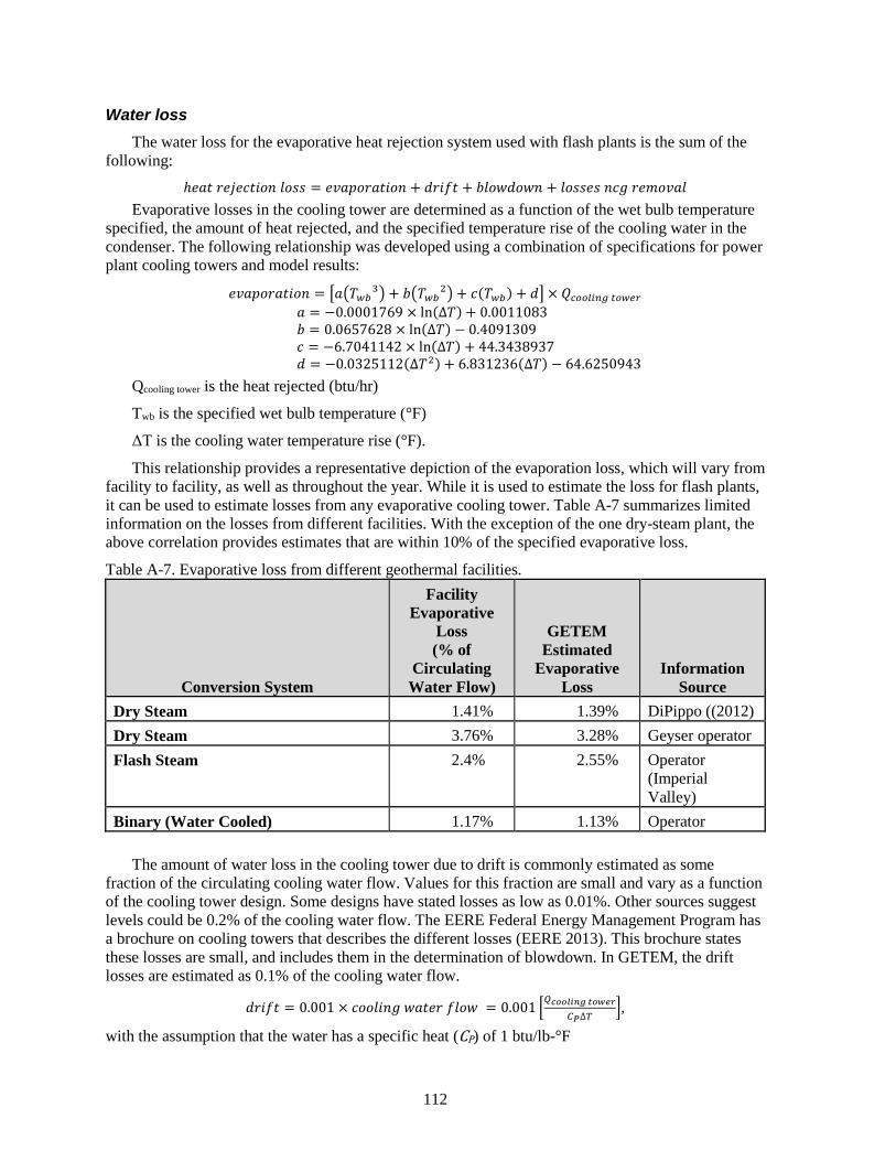
112

Water loss The water loss for the evaporative heat rejection system used with flash plants is the sum of the

following: ℎ𝑃𝑃𝑆𝑆𝑃𝑃 𝑃𝑃𝑃𝑃𝑝𝑝𝑃𝑃𝑃𝑃𝑃𝑃𝑃𝑃𝑃𝑃𝑃𝑃 𝑆𝑆𝑃𝑃𝑆𝑆𝑆𝑆 = 𝑃𝑃𝑙𝑙𝑆𝑆𝑃𝑃𝑃𝑃𝑃𝑃𝑆𝑆𝑃𝑃𝑃𝑃𝑃𝑃𝑃𝑃 + 𝑑𝑑𝑃𝑃𝑃𝑃𝑓𝑓𝑃𝑃 + 𝑏𝑏𝑆𝑆𝑃𝑃𝑃𝑃𝑑𝑑𝑃𝑃𝑃𝑃𝑃𝑃 + 𝑆𝑆𝑃𝑃𝑆𝑆𝑆𝑆𝑃𝑃𝑆𝑆 𝑃𝑃𝑃𝑃𝑃𝑃 𝑃𝑃𝑃𝑃𝑃𝑃𝑃𝑃𝑙𝑙𝑆𝑆𝑆𝑆

Evaporative losses in the cooling tower are determined as a function of the wet bulb temperature specified, the amount of heat rejected, and the specified temperature rise of the cooling water in the condenser. The following relationship was developed using a combination of specifications for power plant cooling towers and model results:

𝑃𝑃𝑙𝑙𝑆𝑆𝑃𝑃𝑃𝑃𝑃𝑃𝑆𝑆𝑃𝑃𝑃𝑃𝑃𝑃𝑃𝑃 = �𝑆𝑆�𝑇𝑇𝑤𝑤𝑏𝑏3� + 𝑏𝑏�𝑇𝑇𝑤𝑤𝑏𝑏2� + 𝑃𝑃(𝑇𝑇𝑤𝑤𝑏𝑏) + 𝑑𝑑� × 𝑄𝑄𝑎𝑎𝑔𝑔𝑔𝑔𝑓𝑓𝑓𝑓𝑛𝑛𝑔𝑔 𝑛𝑛𝑔𝑔𝑤𝑤𝑛𝑛𝑝𝑝 𝑆𝑆 = −0.0001769 × ln(∆𝑇𝑇) + 0.0011083 𝑏𝑏 = 0.0657628 × ln(∆𝑇𝑇) − 0.4091309 𝑃𝑃 = −6.7041142 × ln(∆𝑇𝑇) + 44.3438937 𝑑𝑑 = −0.0325112(∆𝑇𝑇2) + 6.831236(∆𝑇𝑇) − 64.6250943

Qcooling tower is the heat rejected (btu/hr)

Twb is the specified wet bulb temperature (°F)

ΔT is the cooling water temperature rise (°F).

This relationship provides a representative depiction of the evaporation loss, which will vary from facility to facility, as well as throughout the year. While it is used to estimate the loss for flash plants, it can be used to estimate losses from any evaporative cooling tower. Table A-7 summarizes limited information on the losses from different facilities. With the exception of the one dry-steam plant, the above correlation provides estimates that are within 10% of the specified evaporative loss.

Table A-7. Evaporative loss from different geothermal facilities.

Conversion System

Facility Evaporative

Loss (% of

Circulating Water Flow)

GETEM Estimated

Evaporative Loss

Information Source

Dry Steam 1.41% 1.39% DiPippo ((2012) Dry Steam 3.76% 3.28% Geyser operator Flash Steam 2.4% 2.55% Operator

(Imperial Valley)

Binary (Water Cooled) 1.17% 1.13% Operator

The amount of water loss in the cooling tower due to drift is commonly estimated as some fraction of the circulating cooling water flow. Values for this fraction are small and vary as a function of the cooling tower design. Some designs have stated losses as low as 0.01%. Other sources suggest levels could be 0.2% of the cooling water flow. The EERE Federal Energy Management Program has a brochure on cooling towers that describes the different losses (EERE 2013). This brochure states these losses are small, and includes them in the determination of blowdown. In GETEM, the drift losses are estimated as 0.1% of the cooling water flow.

𝑑𝑑𝑃𝑃𝑃𝑃𝑓𝑓𝑃𝑃 = 0.001 × 𝑃𝑃𝑃𝑃𝑃𝑃𝑆𝑆𝑃𝑃𝑃𝑃𝑃𝑃 𝑃𝑃𝑆𝑆𝑃𝑃𝑃𝑃𝑃𝑃 𝑓𝑓𝑆𝑆𝑃𝑃𝑃𝑃 = 0.001 �𝑄𝑄𝑒𝑒𝑜𝑜𝑜𝑜𝑖𝑖𝑖𝑖𝑖𝑖𝑔𝑔 𝑠𝑠𝑜𝑜𝑡𝑡𝑒𝑒𝑟𝑟

𝐿𝐿𝑃𝑃∆𝑇𝑇�,

with the assumption that the water has a specific heat (CP) of 1 btu/lb-°F

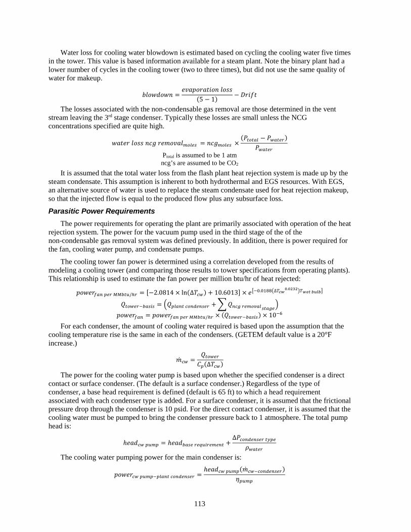
113

Water loss for cooling water blowdown is estimated based on cycling the cooling water five times in the tower. This value is based information available for a steam plant. Note the binary plant had a lower number of cycles in the cooling tower (two to three times), but did not use the same quality of water for makeup.

𝑏𝑏𝑆𝑆𝑃𝑃𝑃𝑃𝑑𝑑𝑃𝑃𝑃𝑃𝑃𝑃 =𝑃𝑃𝑙𝑙𝑆𝑆𝑃𝑃𝑃𝑃𝑃𝑃𝑆𝑆𝑃𝑃𝑃𝑃𝑃𝑃𝑃𝑃 𝑆𝑆𝑃𝑃𝑆𝑆𝑆𝑆

(5 − 1) − 𝐷𝐷𝑃𝑃𝑃𝑃𝑓𝑓𝑃𝑃

The losses associated with the non-condensable gas removal are those determined in the vent stream leaving the 3rd stage condenser. Typically these losses are small unless the NCG concentrations specified are quite high.

𝑃𝑃𝑆𝑆𝑃𝑃𝑃𝑃𝑃𝑃 𝑆𝑆𝑃𝑃𝑆𝑆𝑆𝑆 𝑃𝑃𝑃𝑃𝑃𝑃 𝑃𝑃𝑃𝑃𝑃𝑃𝑃𝑃𝑙𝑙𝑆𝑆𝑆𝑆𝑝𝑝𝑔𝑔𝑓𝑓𝑛𝑛𝑑𝑑 = 𝑃𝑃𝑃𝑃𝑃𝑃𝑝𝑝𝑔𝑔𝑓𝑓𝑛𝑛𝑑𝑑 ×(𝑃𝑃𝑛𝑛𝑔𝑔𝑛𝑛𝑝𝑝𝑓𝑓 − 𝑃𝑃𝑤𝑤𝑝𝑝𝑛𝑛𝑛𝑛𝑝𝑝)

𝑃𝑃𝑤𝑤𝑝𝑝𝑛𝑛𝑛𝑛𝑝𝑝

Ptotal is assumed to be 1 atm ncg’s are assumed to be CO2

It is assumed that the total water loss from the flash plant heat rejection system is made up by the steam condensate. This assumption is inherent to both hydrothermal and EGS resources. With EGS, an alternative source of water is used to replace the steam condensate used for heat rejection makeup, so that the injected flow is equal to the produced flow plus any subsurface loss.

Parasitic Power Requirements The power requirements for operating the plant are primarily associated with operation of the heat

rejection system. The power for the vacuum pump used in the third stage of the of the non-condensable gas removal system was defined previously. In addition, there is power required for the fan, cooling water pump, and condensate pumps.

The cooling tower fan power is determined using a correlation developed from the results of modeling a cooling tower (and comparing those results to tower specifications from operating plants). This relationship is used to estimate the fan power per million btu/hr of heat rejected:

𝑃𝑃𝑃𝑃𝑃𝑃𝑃𝑃𝑃𝑃𝑓𝑓𝑝𝑝𝑛𝑛 𝑝𝑝𝑛𝑛𝑝𝑝 𝑀𝑀𝑀𝑀𝑏𝑏𝑛𝑛𝑓𝑓/ℎ𝑝𝑝 = [−2.0814 × ln(∆𝑇𝑇𝑎𝑎𝑤𝑤) + 10.6013] × 𝑃𝑃�−0.0188�∆𝑇𝑇𝑒𝑒𝑡𝑡0.0232�𝑇𝑇𝑡𝑡𝑒𝑒𝑠𝑠 𝑏𝑏𝑜𝑜𝑖𝑖𝑏𝑏�

𝑄𝑄𝑛𝑛𝑔𝑔𝑤𝑤𝑛𝑛𝑝𝑝−𝑏𝑏𝑝𝑝𝑑𝑑𝑓𝑓𝑑𝑑 = �𝑄𝑄𝑝𝑝𝑓𝑓𝑝𝑝𝑛𝑛𝑛𝑛 𝑎𝑎𝑔𝑔𝑛𝑛𝑓𝑓𝑛𝑛𝑛𝑛𝑑𝑑𝑛𝑛𝑝𝑝 + �𝑄𝑄𝑛𝑛𝑎𝑎𝑔𝑔 𝑝𝑝𝑛𝑛𝑝𝑝𝑔𝑔𝑎𝑎𝑝𝑝𝑓𝑓𝑑𝑑𝑛𝑛𝑝𝑝𝑔𝑔𝑛𝑛�

𝑃𝑃𝑃𝑃𝑃𝑃𝑃𝑃𝑃𝑃𝑓𝑓𝑝𝑝𝑛𝑛 = 𝑃𝑃𝑃𝑃𝑃𝑃𝑃𝑃𝑃𝑃𝑓𝑓𝑝𝑝𝑛𝑛 𝑝𝑝𝑛𝑛𝑝𝑝 𝑀𝑀𝑀𝑀𝑏𝑏𝑛𝑛𝑓𝑓/ℎ𝑝𝑝 × (𝑄𝑄𝑛𝑛𝑔𝑔𝑤𝑤𝑛𝑛𝑝𝑝−𝑏𝑏𝑝𝑝𝑑𝑑𝑓𝑓𝑑𝑑) × 10−6

For each condenser, the amount of cooling water required is based upon the assumption that the cooling temperature rise is the same in each of the condensers. (GETEM default value is a 20°F increase.)

��𝑃𝑎𝑎𝑤𝑤 =𝑄𝑄𝑛𝑛𝑔𝑔𝑤𝑤𝑛𝑛𝑝𝑝𝐿𝐿𝑝𝑝(∆𝑇𝑇𝑎𝑎𝑤𝑤)

The power for the cooling water pump is based upon whether the specified condenser is a direct contact or surface condenser. (The default is a surface condenser.) Regardless of the type of condenser, a base head requirement is defined (default is 65 ft) to which a head requirement associated with each condenser type is added. For a surface condenser, it is assumed that the frictional pressure drop through the condenser is 10 psid. For the direct contact condenser, it is assumed that the cooling water must be pumped to bring the condenser pressure back to 1 atmosphere. The total pump head is:

ℎ𝑃𝑃𝑆𝑆𝑑𝑑𝑎𝑎𝑤𝑤 𝑝𝑝𝑓𝑓𝑝𝑝𝑝𝑝 = ℎ𝑃𝑃𝑆𝑆𝑑𝑑𝑏𝑏𝑝𝑝𝑑𝑑𝑛𝑛 𝑝𝑝𝑛𝑛𝑟𝑟𝑓𝑓𝑓𝑓𝑝𝑝𝑛𝑛𝑝𝑝𝑛𝑛𝑛𝑛𝑛𝑛 +∆𝑃𝑃𝑎𝑎𝑔𝑔𝑛𝑛𝑓𝑓𝑛𝑛𝑛𝑛𝑑𝑑𝑛𝑛𝑝𝑝 𝑛𝑛𝑎𝑎𝑝𝑝𝑛𝑛

𝜌𝜌𝑤𝑤𝑝𝑝𝑛𝑛𝑛𝑛𝑝𝑝

The cooling water pumping power for the main condenser is:

𝑃𝑃𝑃𝑃𝑃𝑃𝑃𝑃𝑃𝑃𝑎𝑎𝑤𝑤 𝑝𝑝𝑓𝑓𝑝𝑝𝑝𝑝−𝑝𝑝𝑓𝑓𝑝𝑝𝑛𝑛𝑛𝑛 𝑎𝑎𝑔𝑔𝑛𝑛𝑓𝑓𝑛𝑛𝑛𝑛𝑑𝑑𝑛𝑛𝑝𝑝 =ℎ𝑃𝑃𝑆𝑆𝑑𝑑𝑎𝑎𝑤𝑤 𝑝𝑝𝑓𝑓𝑝𝑝𝑝𝑝(��𝑃𝑎𝑎𝑤𝑤−𝑎𝑎𝑔𝑔𝑛𝑛𝑓𝑓𝑛𝑛𝑛𝑛𝑑𝑑𝑛𝑛𝑝𝑝)

𝜂𝜂𝑝𝑝𝑓𝑓𝑝𝑝𝑝𝑝

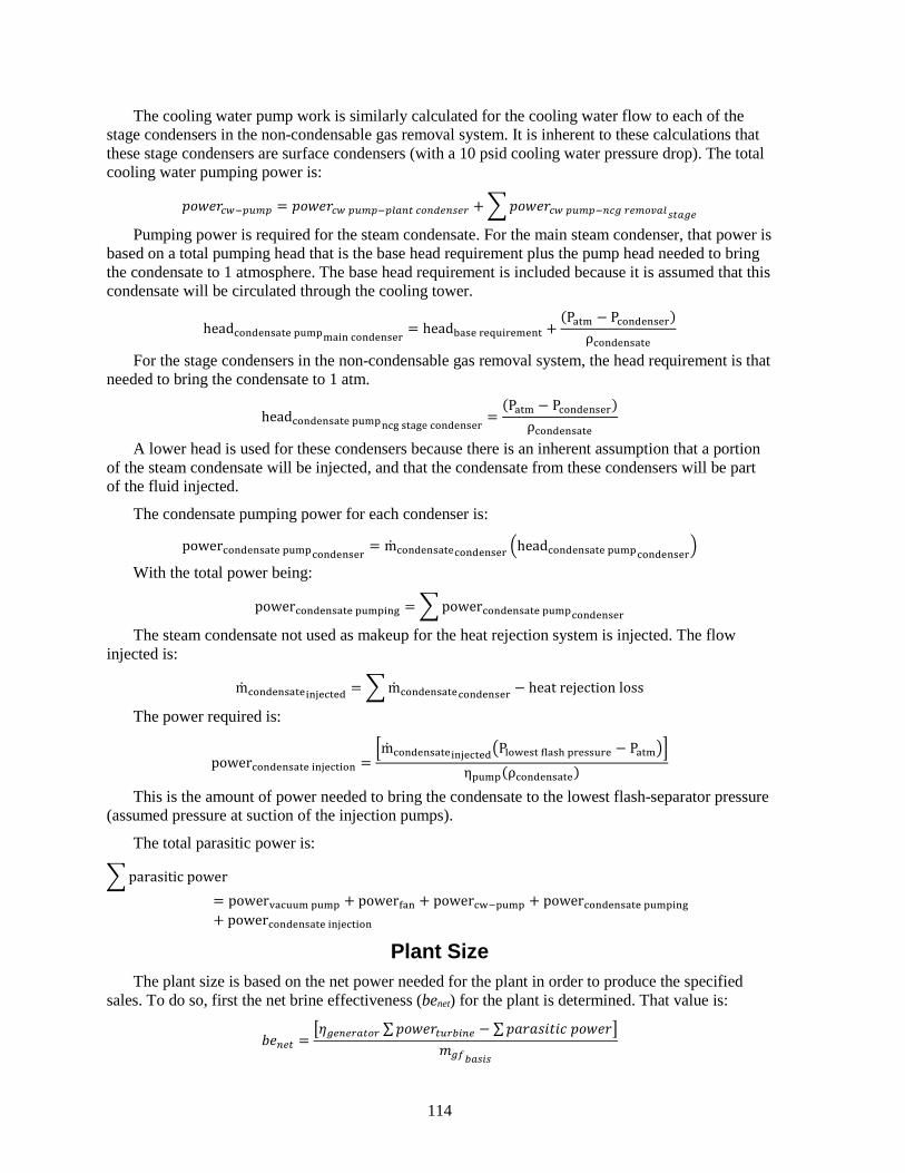
114

The cooling water pump work is similarly calculated for the cooling water flow to each of the stage condensers in the non-condensable gas removal system. It is inherent to these calculations that these stage condensers are surface condensers (with a 10 psid cooling water pressure drop). The total cooling water pumping power is:

𝑃𝑃𝑃𝑃𝑃𝑃𝑃𝑃𝑃𝑃𝑎𝑎𝑤𝑤−𝑝𝑝𝑓𝑓𝑝𝑝𝑝𝑝 = 𝑃𝑃𝑃𝑃𝑃𝑃𝑃𝑃𝑃𝑃𝑎𝑎𝑤𝑤 𝑝𝑝𝑓𝑓𝑝𝑝𝑝𝑝−𝑝𝑝𝑓𝑓𝑝𝑝𝑛𝑛𝑛𝑛 𝑎𝑎𝑔𝑔𝑛𝑛𝑓𝑓𝑛𝑛𝑛𝑛𝑑𝑑𝑛𝑛𝑝𝑝 + �𝑃𝑃𝑃𝑃𝑃𝑃𝑃𝑃𝑃𝑃𝑎𝑎𝑤𝑤 𝑝𝑝𝑓𝑓𝑝𝑝𝑝𝑝−𝑛𝑛𝑎𝑎𝑔𝑔 𝑝𝑝𝑛𝑛𝑝𝑝𝑔𝑔𝑎𝑎𝑝𝑝𝑓𝑓𝑑𝑑𝑛𝑛𝑝𝑝𝑔𝑔𝑛𝑛

Pumping power is required for the steam condensate. For the main steam condenser, that power is based on a total pumping head that is the base head requirement plus the pump head needed to bring the condensate to 1 atmosphere. The base head requirement is included because it is assumed that this condensate will be circulated through the cooling tower.

headcondensate pumpmain condenser= headbase requirement +

(Patm − Pcondenser)ρcondensate

For the stage condensers in the non-condensable gas removal system, the head requirement is that needed to bring the condensate to 1 atm.

headcondensate pumpncg stage condenser=

(Patm − Pcondenser)ρcondensate

A lower head is used for these condensers because there is an inherent assumption that a portion of the steam condensate will be injected, and that the condensate from these condensers will be part of the fluid injected.

The condensate pumping power for each condenser is:

powercondensate pumpcondenser= mcondensatecondenser �headcondensate pumpcondenser

�

With the total power being:

powercondensate pumping = � powercondensate pumpcondenser

The steam condensate not used as makeup for the heat rejection system is injected. The flow injected is:

mcondensateinjected = � mcondensatecondenser − heat rejection loss

The power required is:

powercondensate injection =�mcondensateinjected�Plowest flash pressure − Patm��

ηpump(ρcondensate)

This is the amount of power needed to bring the condensate to the lowest flash-separator pressure (assumed pressure at suction of the injection pumps).

The total parasitic power is:

� parasitic power= powervacuum pump + powerfan + powercw−pump + powercondensate pumping+ powercondensate injection

Plant Size The plant size is based on the net power needed for the plant in order to produce the specified

sales. To do so, first the net brine effectiveness (benet) for the plant is determined. That value is:

𝑏𝑏𝑃𝑃𝑛𝑛𝑛𝑛𝑛𝑛 =�𝜂𝜂𝑔𝑔𝑛𝑛𝑛𝑛𝑛𝑛𝑝𝑝𝑝𝑝𝑛𝑛𝑔𝑔𝑝𝑝 ∑ 𝑃𝑃𝑃𝑃𝑃𝑃𝑃𝑃𝑃𝑃𝑛𝑛𝑓𝑓𝑝𝑝𝑏𝑏𝑓𝑓𝑛𝑛𝑛𝑛 − ∑𝑃𝑃𝑆𝑆𝑃𝑃𝑆𝑆𝑆𝑆𝑃𝑃𝑃𝑃𝑃𝑃𝑃𝑃 𝑃𝑃𝑃𝑃𝑃𝑃𝑃𝑃𝑃𝑃�

𝑃𝑃𝑔𝑔𝑓𝑓𝑏𝑏𝑝𝑝𝑑𝑑𝑓𝑓𝑑𝑑

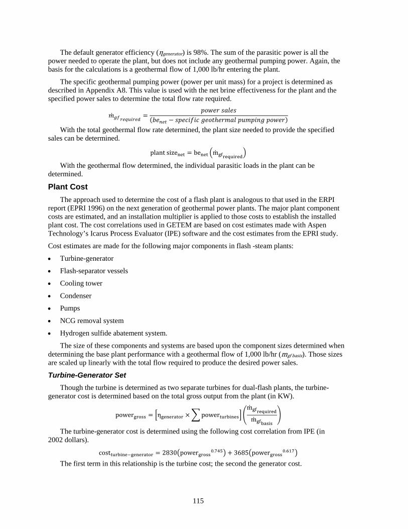
115

The default generator efficiency (ηgenerator) is 98%. The sum of the parasitic power is all the power needed to operate the plant, but does not include any geothermal pumping power. Again, the basis for the calculations is a geothermal flow of 1,000 lb/hr entering the plant.

The specific geothermal pumping power (power per unit mass) for a project is determined as described in Appendix A8. This value is used with the net brine effectiveness for the plant and the specified power sales to determine the total flow rate required.

��𝑃𝑔𝑔𝑓𝑓𝑝𝑝𝑛𝑛𝑟𝑟𝑓𝑓𝑓𝑓𝑝𝑝𝑛𝑛𝑓𝑓=

𝑃𝑃𝑃𝑃𝑃𝑃𝑃𝑃𝑃𝑃 𝑆𝑆𝑆𝑆𝑆𝑆𝑃𝑃𝑆𝑆(𝑏𝑏𝑃𝑃𝑛𝑛𝑛𝑛𝑛𝑛 − 𝑆𝑆𝑃𝑃𝑃𝑃𝑃𝑃𝑃𝑃𝑓𝑓𝑃𝑃𝑃𝑃 𝑃𝑃𝑃𝑃𝑃𝑃𝑃𝑃ℎ𝑃𝑃𝑃𝑃𝑃𝑃𝑆𝑆𝑆𝑆 𝑃𝑃𝑃𝑃𝑃𝑃𝑃𝑃𝑃𝑃𝑃𝑃𝑃𝑃 𝑃𝑃𝑃𝑃𝑃𝑃𝑃𝑃𝑃𝑃)

With the total geothermal flow rate determined, the plant size needed to provide the specified sales can be determined.

plant sizenet = benet �mgfrequired�

With the geothermal flow determined, the individual parasitic loads in the plant can be determined.

Plant Cost The approach used to determine the cost of a flash plant is analogous to that used in the ERPI

report (EPRI 1996) on the next generation of geothermal power plants. The major plant component costs are estimated, and an installation multiplier is applied to those costs to establish the installed plant cost. The cost correlations used in GETEM are based on cost estimates made with Aspen Technology’s Icarus Process Evaluator (IPE) software and the cost estimates from the EPRI study.

Cost estimates are made for the following major components in flash -steam plants:

• Turbine-generator

• Flash-separator vessels

• Cooling tower

• Condenser

• Pumps

• NCG removal system

• Hydrogen sulfide abatement system.

The size of these components and systems are based upon the component sizes determined when determining the base plant performance with a geothermal flow of 1,000 lb/hr (mgf basis). Those sizes are scaled up linearly with the total flow required to produce the desired power sales.

Turbine-Generator Set Though the turbine is determined as two separate turbines for dual-flash plants, the turbine-

generator cost is determined based on the total gross output from the plant (in KW).

powergross = �ηgenerator × � powerturbines� �mgfrequired

mgfbasis

�

The turbine-generator cost is determined using the following cost correlation from IPE (in 2002 dollars).

costturbine−generator = 2830�powergross0.745� + 3685�powergross0.617� The first term in this relationship is the turbine cost; the second the generator cost.

116

Cooling Tower The estimated cost (in 2002 dollars) of the cooling tower is based on the amount of heat that is

rejected (Qreject) from the tower. This value is determined by multiplying the value for the amount of heat rejected (that was determined when establishing the plant performance by the ratio of the geothermal fluid flow rate required) to that used when determining performance (1,000 lb/hr).

Qreject = Qtower−basis �mgfrequired

mgfbasis

�

costcooling tower = 7800�Qreject0.8�

Condenser The condenser cost is estimated (in 2002 dollars) for either a surface condenser or a direct contact

condenser. The surface condenser size is estimated based on the heat rejected in the main steam condenser and the defaults used for the cooling water temperature rise (20°F), the minimum approach temperature between the cooling water and the steam (7.5°F), and the overall heat transfer coefficient U (350 btu/hr-ft2-°F). (GTO can adjust these defaults on the DEFAUT Inputs worksheet.) The heat load in the condenser is determined in a similar manner to the cooling tower heat load; the heat load found when establishing plant performance is multiplied by the ratio of the geothermal flow required to that used when determining performance.

areasurface condenser =Qcondenser

U(LMTD)

The LMTD is the log mean temperature difference that is determined from the water temperature rise and the approach temperature (assuming no de-superheating or subcooling of the steam). The correlation used to estimate cost as a function of size was derived from IPE cost estimates of heat exchangers with stainless steel tubes.

costsurface condenser = 102(areasurface condenser0.85)

If a direct contact condenser is used, its cost is estimated using the correlation below, which was developed from estimates in the 1996 EPRI study (EPRI 1996) after bringing the EPRI estimates to 2002 using the Bureau of Labor Statistics Producer Price Index (United States Department of Labor) for process equipment.

costdirect contact condenser = Qcondenser × �1.25�Tgf� + 1480�

In this relationship, the geothermal temperature (Tgf) is in °C; it is the resource temperature less the temperature loss in the well (i.e., the temperature before flashing occurs in the well). The condenser heat load (Qcondenser) in this relationship is in millions of btu per hr.

Pump The pump cost used is the sum of the cooling water pump cost and the condensate pump costs.

The pumping power for both were estimated in determining the plant performance with the base geothermal flow (1,000 lb/hr). The actual power required for each is determined by multiplying the power determined in the performance calculations by the ratio of the required brine flow to that used in the performance calculations. The same cost correlation is used for each pump type.

costcw pump = 2.35 ∗ 1185�powercw pump0.767�

costcondensate pump = 2.35 ∗ 1185�powercondensate pump0.767�

This cost correlation is from IPE estimates of pump costs as a function of power, with power expressed as horsepower. The 2.35 multiplier used in both relationships is the added cost for a stainless steel pump.

costpump = costcw pump + costcondensate pump

117

This pump cost is in 2002 dollars.

Non-Condensable Gas Removal System The cost of the non-condensable gas removal system is based on the type of removal system

being used. (The default is a hybrid system.) Four component costs are determined: vacuum pump, condensers, condensate pumps, and steam ejectors. These components were sized for the geothermal flow rate used to determine the flash plant performance, with their final size varying directly with the ratio of the flow required to that used to determine performance.

Vacuum Pump

The vacuum pump cost for each stage having a vacuum pump is:

If vacuum pump power is less than 5,000 kW:

costvacuum pumpstage= 70000�powervacuum pump

0.34�

else costvacuum pumpstage

= 7400�powervacuum pump0.6�

In these relationships, the vacuum pump power is in kW. The costs are based on IPE estimates in 2002 dollars and include the cost of the motor. The total vacuum pump cost is:

costvacuum pump = � costvacuum pumpstage

The default is to use a vacuum pump for only the third stage. Though this is not a default that can be revised, GTO can revise inputs to use all vacuum pumps or to use all steam ejectors.

Condenser

The stage condenser costs are based on the heat load for that stage, and the U and LMTD used to determine the plant steam condenser cost. The relationship for the cost of each condenser is based on IPE costs that are in 2002 dollars, and assumes the use of stainless steel tubes.

costcondenserstage = 322(areacondenser0.6)

The total condenser cost is the sum of the costs determined for each stage:

costncg condensers = � costcondenserstage

Condensate Pumps

The same relationship used to estimate the costs for the cooling water and main condenser steam condensate pumps is also used to estimate costs of the steam condensate pumps used to bring the condensate from the non-condensable removal system to 1 atm. These pumps are used for the first and second stages, but not the third, during which condensation occurs at 1 atmosphere.

costcondensate pumpstage= 2.35 ∗ 1185�powercondensate pump

0.767�

Again, the pumps are stainless steel and the power used is the pump’s horsepower. The total cost for the condensate pumps is:

costncg condensate pumps = � costcondensate pumpstage

Steam Ejectors

The steam ejector costs are also based on correlations developed from IPE estimates in 2002 dollars. The costs are based on the ratio of the supply steam pressure to the suction pressure and the non-condensable gas flow (lb/hr). A relationship is developed for each of the three stages.

118

First stage:

costejector−stage 1 = mncg �76 �Psupply steam

Psuction−stage 1�−0.45

�

Second stage:

costejector−stage 2 = mncg �43 �Psupply steam

Psuction−stage 2�−0.63

�

Third stage (not default):

costejector−stage 3 = mncg �43 �Psupply steam

Psuction−stage 3�−0.63

�

The total cost for the steam ejectors is:

costncg ejectors = � costejectorstage

The total cost for the non-condensable gas removal system is: costncg removal = costvacuum pump + costncg condensers + costncg condensate pumps + 𝐿𝐿𝑃𝑃𝑆𝑆𝑃𝑃𝑃𝑃𝑃𝑃𝑃𝑃 𝑃𝑃𝑝𝑝𝑃𝑃𝑃𝑃𝑃𝑃𝑃𝑃𝑃𝑃𝑆𝑆

Hydrogen Sulfide Abatement Minimal information exists upon which to base the cost for abatement of hydrogen sulfide. The

estimate made is based on cost information in the 1995 ERPI Next Generation Geothermal Power Plant study after bringing those estimates to 2002 using the Bureau of Labor Statistics Producer Price Index for process equipment.

costH2S Abatement = 115000�mH2S0.58�

In this relationship, the H2S flow (mH2S) is the flow in lb/hr

Flash-Separator Vessels The flash-separator vessel cost is based on the steam flow and a specified maximum entrained

liquid water drop size. The flash–separator pressure and steam mass flow from that vessel determines the volumetric flow rate. For the specified droplet size (the default is a 200-micron diameter), the following relationship is used to determine its settling velocity. (This was derived from a curve fit of calculated velocities for a range of conditions.)

Vsettling = 0.009414�Ddrop2�[ln(Pflash)] + 0.1096�Ddrop

2� where

Vsettling is settling velocity in ft/s

Ddrop is drop diameter in inches

Pflash is flash pressure in psia.

The area of the flash vessel is

A =�msteam−flash ρsteam−flash

� �Vsettling

An arbitrary limit of 300 ft2 is placed on the separator cross-sectional area—if larger, two vessels are required. It is assumed that the vessel height is three times its diameter. The height and diameter are used to determine the volume of the vessel in gallons. This capacity is used to estimate cost (in 2002 dollars).

119

If Pflash <75 psia Costflash−separator = 166.5�Capacityvessel−gal0.625�

Else

Costflash−separator = 110�Capacityvessel−gal0.68� These costs were derived from IPE estimates of pressure vessels. These correlations are used for

both the high- and low-pressure flash-separator vessels. If multiple vessels are required at either flash level, the size of an individual vessel is determined and a cost estimated for that size. The cost of the flash-separator vessels at that flash level is this cost multiplied by the number of vessels needed.

Total Flash Plant Cost The cost estimates for the major plant components are in 2002 dollars. They are adjusted to the

year for which the GETEM estimate is being made using the PPIs from the Bureau of Labor Statistics. Once applied, a total cost is found for the major equipment items. Using an approach that is analogous to that in the EPRI report (EPRI 1996), a multiplier is applied to these costs to get a total installed cost at the start of operation.

installed plant cost = installation multiplier × � PPI�costmajor equipment�

The installation multiplier is determined as: installation multiplier = multiplierdirect construction(1 + indirect cost multiplier)

Both the direct construction multiplier and the indirect cost multiplier are specified inputs that can be revised. The default value for the direct construction multiplier is determined using an approach based on IPE estimates for flash steam power plants. The multiplier consists of:

− Other materials − Labor − Other construction (on-site construction management/supervision, construction expendables,

and rentals) − Tax − Freight

The other materials include the cost of steel, piping, concrete, electrical equipment, instrumentation, insulation, paint, buildings, and similar things needed during plant construction. The value used is derived from the IPE estimates as a function of the resource temperature (°C) less temperature loss in the well bore. The multiplier for the total material costs varies inversely with this temperature; the value used is:

total materials multiplier2002 = 8.65�Tgf−0.297� This value, multiplied by the major component costs, is the total materials costs for the project,

including the “other materials.” The contributors to the direct construction multiplier are based on the major component costs in 2002 dollars. Though the magnitude of all contributions to the construction multiplier are adjusted using PPIs, this multiplier is applied to equipment costs that have unique PPIs as well. To account for the effect that the equipment PPIs would otherwise have on the contribution of these other costs, an effective PPI is determined for the major component costs. This value is then used to adjust the effect of the PPIs applied to each of the contributors to direct the construction cost multiplier. This adjustment is determined as:

major component cost adjustment, or MCCA =∑�component cost2002�PPIcomponent��

∑ component cost2002

120

The PPI for process equipment is applied to the “other materials” contribution and corrected with the above adjustment to remove the effects of changes to the major equipment costs. The resulting total materials multiplier is:

total materials multiplier = 1 + (total materials multiplier2002 − 1) �PPIprocess equipment

MCCA�

This multiplier is used to determine the total material costs for the plant construction for the year of the estimate. This includes major component costs and the “other” materials.

total material costs = total materials multiplier × � component cost2002�PPIcomponent�

The labor cost multiplier component is also derived from IPE estimates as a function of the resource temperature (°C) less well bore losses:

labor multiplier2002 = 61.843�Tgf−0.923� In the year of interest, the multiplier is:

labor multiplier = labor multiplier2002 �PPIlaborMCCA

�

The contribution of construction supervision, expendables, and rentals to the installation multiplier is based on the IPE estimates as well, and is also determined as a function of the resource temperature (°C) less well bore losses.

other construction multiplier2002 = 16.177�Tgf−0.827� In the year of interest, the multiplier is:

other construction multiplier = other construction multiplier2002 �PPIprocess equipment

MCCA�

The taxes and freight rates are default inputs that cannot be revised. They are applied to the material costs and the other construction costs (not to labor).

The direct construction multiplier is: 𝑃𝑃𝑃𝑃𝑆𝑆𝑃𝑃𝑃𝑃𝑃𝑃𝑆𝑆𝑃𝑃𝑃𝑃𝑃𝑃𝑓𝑓𝑓𝑓𝑝𝑝𝑛𝑛𝑎𝑎𝑛𝑛 𝑎𝑎𝑔𝑔𝑛𝑛𝑑𝑑𝑛𝑛𝑝𝑝𝑓𝑓𝑎𝑎𝑛𝑛𝑓𝑓𝑔𝑔𝑛𝑛 = 𝑆𝑆𝑆𝑆𝑏𝑏𝑃𝑃𝑃𝑃 𝑃𝑃𝑃𝑃𝑆𝑆𝑃𝑃𝑃𝑃𝑃𝑃𝑆𝑆𝑃𝑃𝑃𝑃𝑃𝑃 + 𝑃𝑃𝑃𝑃𝑃𝑃𝑆𝑆𝑆𝑆 𝑃𝑃𝑆𝑆𝑃𝑃𝑃𝑃𝑃𝑃𝑃𝑃𝑆𝑆𝑆𝑆𝑆𝑆 𝑃𝑃𝑃𝑃𝑆𝑆𝑃𝑃𝑃𝑃𝑃𝑃𝑆𝑆𝑃𝑃𝑃𝑃𝑃𝑃(1 + 𝑃𝑃𝑆𝑆𝐼𝐼 + 𝑓𝑓𝑃𝑃𝑃𝑃𝑃𝑃𝑃𝑃ℎ𝑃𝑃)

+𝑃𝑃𝑃𝑃ℎ𝑃𝑃𝑃𝑃 𝑃𝑃𝑃𝑃𝑃𝑃𝑆𝑆𝑃𝑃𝑃𝑃𝑃𝑃𝑃𝑃𝑃𝑃𝑃𝑃𝑃𝑃𝑃𝑃 𝑃𝑃𝑃𝑃𝑆𝑆𝑃𝑃𝑃𝑃𝑃𝑃𝑆𝑆𝑃𝑃𝑃𝑃𝑃𝑃(1 + 𝑃𝑃𝑆𝑆𝐼𝐼 + 𝑓𝑓𝑃𝑃𝑃𝑃𝑃𝑃𝑃𝑃ℎ𝑃𝑃) The indirect costs for the plant construction include engineering, home office, startup, and other

activities not directly associated the plant construction. They are determined as a specified (input) fraction of the direct construction costs. (Note that engineering is assumed to be 50% of these indirect costs; in the project schedule, half of these engineering costs are incurred before obtaining the PPA.) The total installation multiplier is:

installation multiplier = multiplierdirect construction(1 + indirect cost multiplier) The total installed plant cost is:

installed plant cost = installation multiplier × � PPI�costmajor equipment�

The following shows values for an example scenario:

- Major component cost (in year of interest), or ∑PPI(costmajor equipment): $10,000,000 - Labor multiplier: 0.4 - Other construction multiplier: 0.2 - Total materials multiplier: 1.8 - Taxes: 0.06 - Freight: 0.05

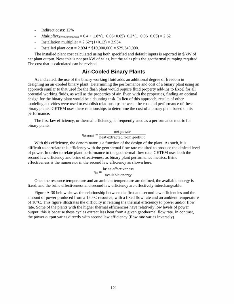
121

- Indirect costs: 12% - Multiplierdirect construction = 0.4 + 1.8*(1+0.06+0.05)+0.2*(1+0.06+0.05) = 2.62 - Installation multiplier = 2.62*(1+0.12) = 2.934 - Installed plant cost = 2.934 * $10,000,000 = $29,340,000. The installed plant cost calculated using both specified and default inputs is reported in $/kW of

net plant output. Note this is not per kW of sales, but the sales plus the geothermal pumping required. The cost that is calculated can be revised.

Air-Cooled Binary Plants As indicated, the use of the binary working fluid adds an additional degree of freedom in

designing an air-cooled binary plant. Determining the performance and cost of a binary plant using an approach similar to that used for the flash plant would require fluid property add-ins to Excel for all potential working fluids, as well as the properties of air. Even with the properties, finding an optimal design for the binary plant would be a daunting task. In lieu of this approach, results of other modeling activities were used to establish relationships between the cost and performance of these binary plants. GETEM uses these relationships to determine the cost of a binary plant based on its performance.

The first law efficiency, or thermal efficiency, is frequently used as a performance metric for binary plants.

ηthermal =net power

heat extracted from geofluid

With this efficiency, the denominator is a function of the design of the plant. As such, it is difficult to correlate this efficiency with the geothermal flow rate required to produce the desired level of power. In order to relate plant performance to the geothermal flow rate, GETEM uses both the second law efficiency and brine effectiveness as binary plant performance metrics. Brine effectiveness is the numerator in the second law efficiency as shown here:

ηII =brine effectivenessavaılable energy

Once the resource temperature and an ambient temperature are defined, the available energy is fixed, and the brine effectiveness and second law efficiency are effectively interchangeable.

Figure A-30 below shows the relationship between the first and second law efficiencies and the amount of power produced from a 150°C resource, with a fixed flow rate and an ambient temperature of 10°C. This figure illustrates the difficulty in relating the thermal efficiency to power and/or flow rate. Some of the plants with the higher thermal efficiencies have relatively low levels of power output; this is because these cycles extract less heat from a given geothermal flow rate. In contrast, the power output varies directly with second law efficiency (flow rate varies inversely).

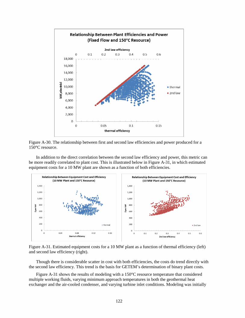
122

Figure A-30. The relationship between first and second law efficiencies and power produced for a 150°C resource.

In addition to the direct correlation between the second law efficiency and power, this metric can be more readily correlated to plant cost. This is illustrated below in Figure A-31, in which estimated equipment costs for a 10 MW plant are shown as a function of both efficiencies.

Figure A-31. Estimated equipment costs for a 10 MW plant as a function of thermal efficiency (left) and second law efficiency (right).

Though there is considerable scatter in cost with both efficiencies, the costs do trend directly with the second law efficiency. This trend is the basis for GETEM’s determination of binary plant costs.

Figure A-31 shows the results of modeling with a 150°C resource temperature that considered multiple working fluids, varying minimum approach temperatures in both the geothermal heat exchanger and the air-cooled condenser, and varying turbine inlet conditions. Modeling was initially

123

done at a fixed geothermal flow rate (5,000 gpm), and those results were used to scale equipment size to a 10 MW net plant output. Both resource and ambient temperatures were held constant, and the condensing temperature varied, given the maximum net output for the specific conditions being evaluated. (Net plant output is the generator output less the working fluid pumping power and fan power required.) Equipment costs were estimated for all modeled scenarios (for 10 MW plants) using correlations developed from Aspen’s IPE estimates.

Resource temperatures from 75°C to 200°C were modeled at increments of 25°C. The working fluids considered were propane, isobutane, normal butane, isopentane, R134a, and R245fa. All plants were modeled having a single vaporizer (dual boiling cycles were not evaluated), with a maximum working fluid turbine inlet pressure of 1,200 psia. Supercritical cycles were modeled; they have both higher levels of performance and higher costs.

Below in Figure A-22 are the equipment cost estimates for the 100°C and 200°C resources as functions of the second law efficiency for the 10 MW net plant. Similar estimates were made for the 75°, 125°, and 175°C resources as well.

Figure A-32. Equipment cost estimates for a 100°C (left) and a 200°C resource (right).

For each resource temperature, the cost estimates were sorted and only those that were approaching the minimum cost at a given level of performance were selected. That down select is shown below in Figure A-33 for the 150°C resource (again, for a 10 MW plant).

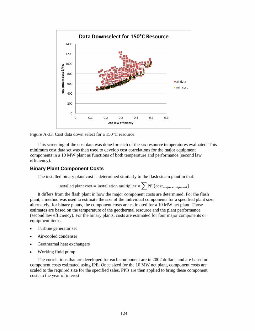
124

Figure A-33. Cost data down select for a 150°C resource.

This screening of the cost data was done for each of the six resource temperatures evaluated. This minimum cost data set was then used to develop cost correlations for the major equipment components in a 10 MW plant as functions of both temperature and performance (second law efficiency).

Binary Plant Component Costs The installed binary plant cost is determined similarly to the flash steam plant in that:

installed plant cost = installation multiplier × � PPI�costmajor equipment�

It differs from the flash plant in how the major component costs are determined. For the flash plant, a method was used to estimate the size of the individual components for a specified plant size; alternately, for binary plants, the component costs are estimated for a 10 MW net plant. Those estimates are based on the temperature of the geothermal resource and the plant performance (second law efficiency). For the binary plants, costs are estimated for four major components or equipment items.

• Turbine generator set

• Air-cooled condenser

• Geothermal heat exchangers

• Working fluid pump.

The correlations that are developed for each component are in 2002 dollars, and are based on component costs estimated using IPE. Once sized for the 10 MW net plant, component costs are scaled to the required size for the specified sales. PPIs are then applied to bring these component costs to the year of interest.

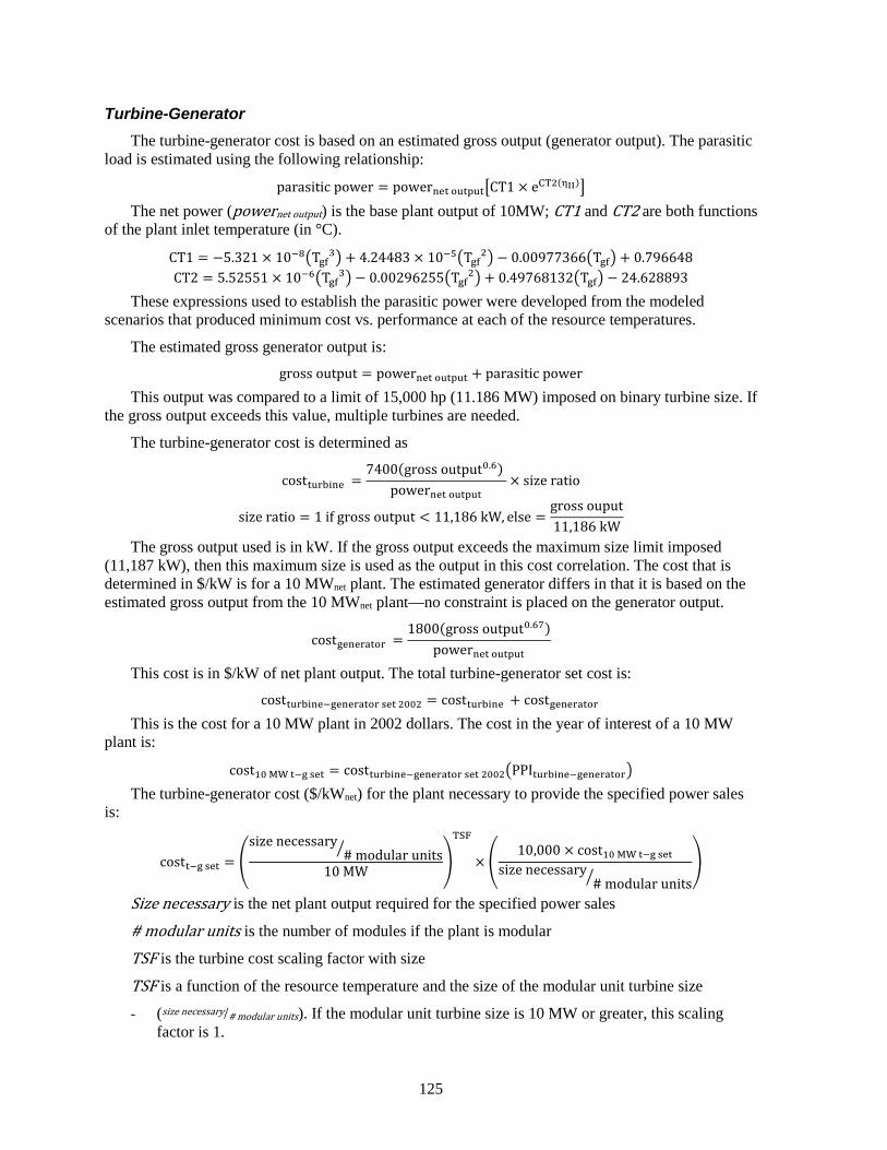
125

Turbine-Generator The turbine-generator cost is based on an estimated gross output (generator output). The parasitic

load is estimated using the following relationship:

parasitic power = powernet output�CT1 × eCT2(ηII)�

The net power (powernet output) is the base plant output of 10MW; CT1 and CT2 are both functions of the plant inlet temperature (in °C).

CT1 = −5.321 × 10−8�Tgf3� + 4.24483 × 10−5�Tgf2� − 0.00977366�Tgf� + 0.796648 CT2 = 5.52551 × 10−6�Tgf3� − 0.00296255�Tgf2� + 0.49768132�Tgf� − 24.628893

These expressions used to establish the parasitic power were developed from the modeled scenarios that produced minimum cost vs. performance at each of the resource temperatures.

The estimated gross generator output is: gross output = powernet output + parasitic power

This output was compared to a limit of 15,000 hp (11.186 MW) imposed on binary turbine size. If the gross output exceeds this value, multiple turbines are needed.

The turbine-generator cost is determined as

costturbine =7400(gross output0.6)

powernet output× size ratio

size ratio = 1 if gross output < 11,186 kW, else =gross ouput11,186 kW

The gross output used is in kW. If the gross output exceeds the maximum size limit imposed (11,187 kW), then this maximum size is used as the output in this cost correlation. The cost that is determined in $/kW is for a 10 MWnet plant. The estimated generator differs in that it is based on the estimated gross output from the 10 MWnet plant—no constraint is placed on the generator output.

costgenerator =1800(gross output0.67)

powernet output

This cost is in $/kW of net plant output. The total turbine-generator set cost is: costturbine−generator set 2002 = costturbine + costgenerator

This is the cost for a 10 MW plant in 2002 dollars. The cost in the year of interest of a 10 MW plant is:

cost10 MW t−g set = costturbine−generator set 2002�PPIturbine−generator� The turbine-generator cost ($/kWnet) for the plant necessary to provide the specified power sales

is:

costt−g set = �size necessary

# modular units�10 MW

�

TSF

× �10,000 × cost10 MW t−g set

size necessary# modular units�

�

Size necessary is the net plant output required for the specified power sales

# modular units is the number of modules if the plant is modular

TSF is the turbine cost scaling factor with size

TSF is a function of the resource temperature and the size of the modular unit turbine size

- (size necessary/# modular units). If the modular unit turbine size is 10 MW or greater, this scaling factor is 1.

126

- If <1, TSF is a function of the resource temperature. It is based on modeled results using the IPE software to estimate plant costs.

TSF = −2.0218 × 10−6�Tgf2� + 0.000358909�Tgf� + 0.6642

This cost (costt-g set) is the cost of the turbine generator for the plant in $/kW for the year of interest. It is adjusted to provide the specified sales and to reflect the use of modular units.

Air-Cooled Condenser The air-cooled condenser costs are also first determined for a 10 MWnet plant. The cost for this

air-cooled condenser is:

costAC condenser−2002 = AC1(ηIIAC2) + AC0 Where AC1, AC2, and AC0 are functions of the geothermal fluid temperature (°C).

𝑃𝑃𝐿𝐿0 = 11568490�𝑇𝑇𝑔𝑔𝑓𝑓−2.35092� + 47

𝑃𝑃𝐿𝐿1 = 𝑃𝑃�5.65748×10−6�𝑇𝑇𝑔𝑔𝑒𝑒3�−0.001200635�𝑇𝑇𝑔𝑔𝑒𝑒2�+0.005950211�𝑇𝑇𝑔𝑔𝑒𝑒�+15.52712�

𝑃𝑃𝐿𝐿2 = 𝑃𝑃�−2.54939×10−7�𝑇𝑇𝑔𝑔𝑒𝑒3�+0.000277465�𝑇𝑇𝑔𝑔𝑒𝑒2�−0.05107826�𝑇𝑇𝑔𝑔𝑒𝑒�+3.584261�

This cost for the air-cooled condenser is again for a 10 MW plant and is in $/kW (2002 dollars). To get this base 10 MW plant cost in the year of interest, a PPI is applied.

𝑃𝑃𝑃𝑃𝑆𝑆𝑃𝑃10 𝑀𝑀𝑘𝑘 𝑃𝑃𝐿𝐿 𝑎𝑎𝑔𝑔𝑛𝑛𝑓𝑓𝑛𝑛𝑛𝑛𝑑𝑑𝑛𝑛𝑝𝑝 = 𝑃𝑃𝑃𝑃𝑆𝑆𝑃𝑃𝑃𝑃𝐿𝐿 𝑎𝑎𝑔𝑔𝑛𝑛𝑓𝑓𝑛𝑛𝑛𝑛𝑑𝑑𝑛𝑛𝑝𝑝−2002�𝑃𝑃𝑃𝑃𝐼𝐼ℎ𝑛𝑛𝑝𝑝𝑛𝑛 𝑛𝑛𝑒𝑒𝑎𝑎ℎ𝑝𝑝𝑛𝑛𝑔𝑔𝑛𝑛𝑝𝑝𝑑𝑑�

A scaling factor is not applied to the cost of these condensers. Cost estimate modeling with IPE indicated that after ~three condenser bays were used, there was little scaling of cost with size. For plants of interest (>5 MW) more than three condenser bays would be required. The condenser cost is equivalent to the base 10 MW plant cost, in $/kW.

𝑃𝑃𝑃𝑃𝑆𝑆𝑃𝑃𝑃𝑃𝐿𝐿 𝑎𝑎𝑔𝑔𝑛𝑛𝑓𝑓𝑛𝑛𝑛𝑛𝑑𝑑𝑛𝑛𝑝𝑝 = 𝑃𝑃𝑃𝑃𝑆𝑆𝑃𝑃10 𝑀𝑀𝑘𝑘 𝑃𝑃𝐿𝐿 𝑎𝑎𝑔𝑔𝑛𝑛𝑓𝑓𝑛𝑛𝑛𝑛𝑑𝑑𝑛𝑛𝑝𝑝

Geothermal Heat Exchanger The geothermal heat exchanger costs are similarly determined. The cost in $/kW for the 10 MW

base plant is:

costGF exchangers−2002 = GHX1 × e[GHX2(ηII)] The values GHX1 and GHX2 are functions of the geothermal fluid temperature (°C).

GHX1 = 2163827753�Tgf−3.8105414� + 5.95 GHX2 = 4.24462 × 10−6�Tgf3� − 0.002356472�Tgf2� + 0.4275955�Tgf� − 22.09917

Again, this cost is in 2002 dollars. They are adjusted to the year of interest (the year for which the estimate is made).

cost10 MW GF exhcnagers = costGF exchangers−2002�PPIheat exchangers� The geothermal heat exchanger costs do scale with size:

costGF exhcnager = �size necessary

# modular units�10 MW

�

GHXSF

× �10,000 × cost10 MW GF exhcnagerssize necessary

# modular units��

The scaling factor for the geothermal heat exchangers (GHXSF) is a function of the resource temperature:

GHXSF = 2.0145 × 10−6�Tgf2� − 0.000760473�Tgf� + 1.01216

127

Working Fluid Pump The relationship used for the base 10 MW plant working fluid pump cost is:

costWF pump−2002 = WFP1 × e[WFP2(ηII)]

The values WFP1 and WFP2 are functions of the geothermal temperature (°C).

WFP1 = 0.0006714�Tgf2� − 0.25379�Tgf� + 32.06071 WFP2 = −0.0001977�Tgf2� + 0.0559291�Tgf� − 0.3329714

A PPI for pumps is applied to get the base plant pump cost in the year of interest.

cost10 MW WF pump = costWF pump−2002�PPIpump� The working fluid pump costs scale with size:

costWF pump = �size necessary

# modular units�10 MW

�

WFPSF

× �10,000 × cost10 MW WF pump

size necessary# modular units�

�

The scaling factor for the working fluid pumps (WFPSF) is given in terms of the resource temperature (°C).

WFPSF = 3.872 × 10−7�Tgf3� − 0.00019008�Tgf2� + 0.029802�Tgf� − 0.7779 The correlations used in GETEM to estimate the major equipment costs are based on those

equipment costs for the minimum cost scenarios for the resource temperatures evaluated. The correlations that were developed were used to estimate the equipment costs for a 10 MW plant at a specified resource temperature. Figure A-34 shows the effectiveness of using this method to approach those minimum costs for 100°, 150°, and 200°C resources.

128

(a)

(b) (c)

Figure A-34. GETEM’s minimum equipment cost estimates as functions of second law efficiency for a 150°C resource (a), a 100°C resource (b), and a 200°C resource (c).

Except at the higher levels of performance with the 200°C resource, the correlations that were developed to determine the major component costs provided estimates that, when summed, provided reasonable approximations of the minimum costs at a given level of performance.

With this approach, the major component costs are determined for the plant size needed for the power sales in the year for which the LCOE estimate is being made.

To get the installed plant cost, the installation multiplier is determined using an approach similar to that used for the flash steam power plant.

129

Total Air-Cooled Binary Plant Cost Using an approach that is analogous to that in the EPRI report (EPRI 1996), a multiplier is

applied to these costs to get a total installed cost at the start of operation.

installed plant cost = installation multiplier × ��costmajor equipment�

The installation multiplier is determined as: 𝑃𝑃𝑃𝑃𝑆𝑆𝑃𝑃𝑆𝑆𝑆𝑆𝑆𝑆𝑆𝑆𝑃𝑃𝑃𝑃𝑃𝑃𝑃𝑃 𝑃𝑃𝑃𝑃𝑆𝑆𝑃𝑃𝑃𝑃𝑃𝑃𝑆𝑆𝑃𝑃𝑃𝑃𝑃𝑃 = 𝑃𝑃𝑃𝑃𝑆𝑆𝑃𝑃𝑃𝑃𝑃𝑃𝑆𝑆𝑃𝑃𝑃𝑃𝑃𝑃𝑓𝑓𝑓𝑓𝑝𝑝𝑛𝑛𝑎𝑎𝑛𝑛 𝑎𝑎𝑔𝑔𝑛𝑛𝑑𝑑𝑛𝑛𝑝𝑝𝑓𝑓𝑎𝑎𝑛𝑛𝑓𝑓𝑔𝑔𝑛𝑛(1 + 𝑃𝑃𝑃𝑃𝑑𝑑𝑃𝑃𝑃𝑃𝑃𝑃𝑃𝑃𝑃𝑃 𝑃𝑃𝑃𝑃𝑆𝑆𝑃𝑃 𝑃𝑃𝑃𝑃𝑆𝑆𝑃𝑃𝑃𝑃𝑃𝑃𝑆𝑆𝑃𝑃𝑃𝑃𝑃𝑃)

Both the direct construction multiplier and the indirect cost multiplier are specified inputs. The default value for the direct construction multiplier is determined using an approach based on IPE estimates for air-cooled binary power plants. The multiplier consists of the following:

− Other materials − Labor − Other construction (on-site construction management/supervision, construction expendables,

and rentals) − Tax − Freight.

The other materials include the cost of steel, piping, concrete, electrical equipment, instrumentation, insulation, paint, buildings, and similar things needed for plant construction. The value used is derived from the IPE estimates. Those estimates indicated this multiplier was approximately 1.7 in the plant scenarios modeled.

total materials multiplier2002 = 1.7 This value is based on major equipment cost estimates in 2002 dollars. To account for the effect

of changes in these equipment costs over time, an effective PPI for the major components is determined and used to adjust for the impact that the individual contributors have to the direct construction cost multiplier.

𝑃𝑃𝑆𝑆𝑝𝑝𝑃𝑃𝑃𝑃 𝑃𝑃𝑃𝑃𝑃𝑃𝑃𝑃𝑃𝑃𝑃𝑃𝑃𝑃𝑃𝑃𝑃𝑃 𝑃𝑃𝑃𝑃𝑆𝑆𝑃𝑃 𝑆𝑆𝑑𝑑𝑝𝑝𝑃𝑃𝑆𝑆𝑃𝑃𝑃𝑃𝑃𝑃𝑃𝑃𝑃𝑃, 𝑃𝑃𝑃𝑃 𝑀𝑀𝐿𝐿𝐿𝐿𝑃𝑃 =∑𝑃𝑃𝑆𝑆𝑝𝑝𝑃𝑃𝑃𝑃 𝑃𝑃𝑃𝑃𝑃𝑃𝑃𝑃𝑃𝑃𝑃𝑃𝑃𝑃𝑃𝑃𝑃𝑃 𝑃𝑃𝑃𝑃𝑆𝑆𝑃𝑃

∑𝑃𝑃𝑆𝑆𝑝𝑝𝑃𝑃𝑃𝑃 𝑃𝑃𝑃𝑃𝑃𝑃𝑃𝑃𝑃𝑃𝑃𝑃𝑃𝑃𝑃𝑃𝑃𝑃 𝑃𝑃𝑃𝑃𝑆𝑆𝑃𝑃2002

This adjustment is applied to the 2002 total materials multiplier and the PPIs for steel and other materials to determine the multiplier to be applied to the major component costs in the year of interest to obtain the total material cost for the binary plant.

total materials multiplier = 1 + �steel multiplier2002(PPIsteel) + other multiplier2002�PPIprocess equipment�

MCCA �

In the 2002 estimates, the total materials multiplier was 1.7. The major equipment contribution was 1. The steel contribution was ~0.22. The “other” contribution was 1.7 −1 −0.22, or 0.48.

𝑃𝑃𝑃𝑃𝑃𝑃𝑆𝑆𝑆𝑆 𝑃𝑃𝑆𝑆𝑃𝑃𝑃𝑃𝑃𝑃𝑃𝑃𝑆𝑆𝑆𝑆 𝑃𝑃𝑃𝑃𝑆𝑆𝑃𝑃𝑆𝑆 = 𝑃𝑃𝑃𝑃𝑃𝑃𝑆𝑆𝑆𝑆 𝑃𝑃𝑆𝑆𝑃𝑃𝑃𝑃𝑃𝑃𝑃𝑃𝑆𝑆𝑆𝑆𝑆𝑆 𝑃𝑃𝑃𝑃𝑆𝑆𝑃𝑃𝑃𝑃𝑃𝑃𝑆𝑆𝑃𝑃𝑃𝑃𝑃𝑃 × �𝑃𝑃𝑆𝑆𝑝𝑝𝑃𝑃𝑃𝑃 𝑃𝑃𝑃𝑃𝑃𝑃𝑃𝑃𝑃𝑃𝑃𝑃𝑃𝑃𝑃𝑃𝑃𝑃 𝑃𝑃𝑃𝑃𝑆𝑆𝑃𝑃

In 2002, the direct labor contribution to the direct construction multiplier was 0.27, with fringe and benefits being 45% of the labor cost:

𝑑𝑑𝑃𝑃𝑃𝑃𝑃𝑃𝑃𝑃𝑃𝑃 𝑆𝑆𝑆𝑆𝑏𝑏𝑃𝑃𝑃𝑃 𝑃𝑃𝑃𝑃𝑆𝑆𝑃𝑃𝑃𝑃𝑃𝑃𝑆𝑆𝑃𝑃𝑃𝑃𝑃𝑃2002 = 0.27 In the year of interest, the multiplier is:

labor multiplier = direct labor multiplier2002 �PPIlaborMCCA

� × (1 + fringe multiplier)

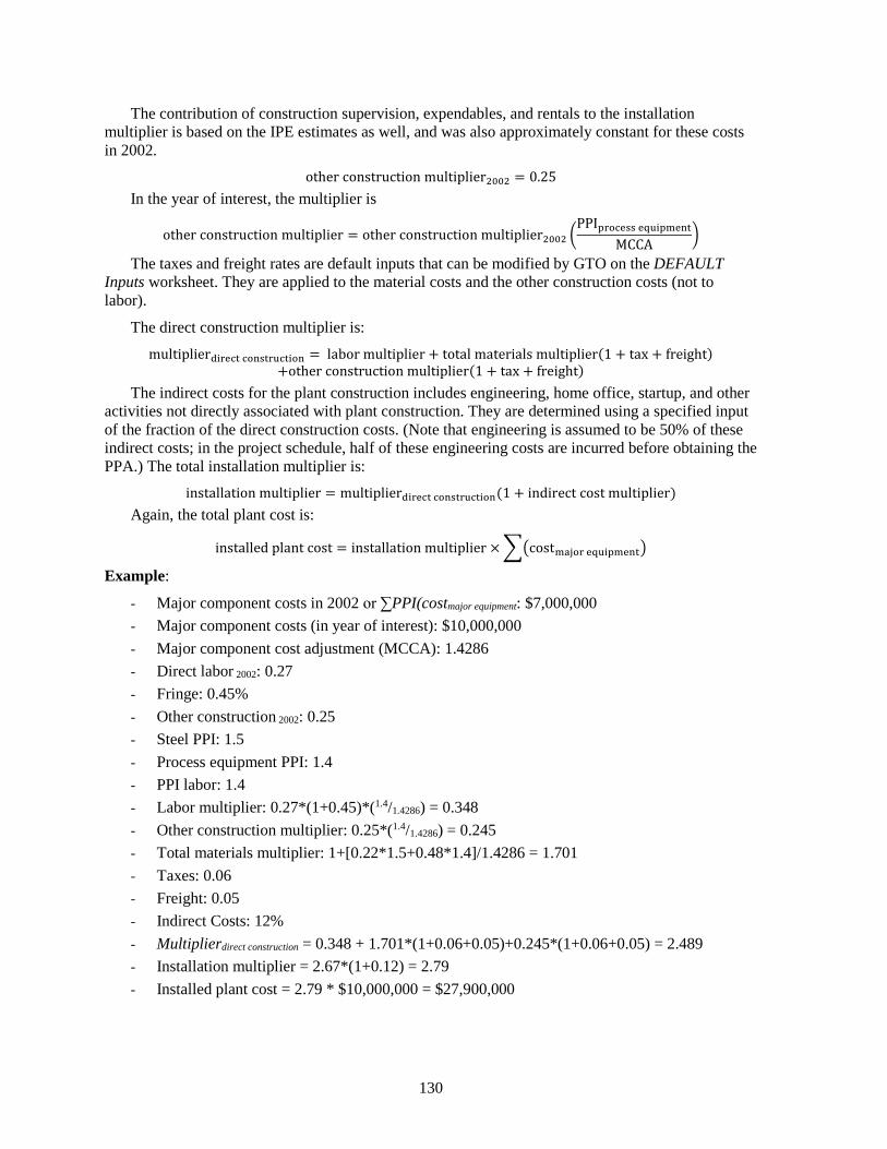
130

The contribution of construction supervision, expendables, and rentals to the installation multiplier is based on the IPE estimates as well, and was also approximately constant for these costs in 2002.

other construction multiplier2002 = 0.25 In the year of interest, the multiplier is

other construction multiplier = other construction multiplier2002 �PPIprocess equipment

MCCA�

The taxes and freight rates are default inputs that can be modified by GTO on the DEFAULT Inputs worksheet. They are applied to the material costs and the other construction costs (not to labor).

The direct construction multiplier is: multiplierdirect construction = labor multiplier + total materials multiplier(1 + tax + freight)

+other construction multiplier(1 + tax + freight) The indirect costs for the plant construction includes engineering, home office, startup, and other

activities not directly associated with plant construction. They are determined using a specified input of the fraction of the direct construction costs. (Note that engineering is assumed to be 50% of these indirect costs; in the project schedule, half of these engineering costs are incurred before obtaining the PPA.) The total installation multiplier is:

installation multiplier = multiplierdirect construction(1 + indirect cost multiplier) Again, the total plant cost is:

installed plant cost = installation multiplier × ��costmajor equipment�

Example:

- Major component costs in 2002 or ∑PPI(costmajor equipment: $7,000,000 - Major component costs (in year of interest): $10,000,000 - Major component cost adjustment (MCCA): 1.4286 - Direct labor 2002: 0.27 - Fringe: 0.45% - Other construction 2002: 0.25 - Steel PPI: 1.5 - Process equipment PPI: 1.4 - PPI labor: 1.4 - Labor multiplier: 0.27*(1+0.45)*(1.4/1.4286) = 0.348 - Other construction multiplier: 0.25*(1.4/1.4286) = 0.245 - Total materials multiplier: 1+[0.22*1.5+0.48*1.4]/1.4286 = 1.701 - Taxes: 0.06 - Freight: 0.05 - Indirect Costs: 12% - Multiplierdirect construction = 0.348 + 1.701*(1+0.06+0.05)+0.245*(1+0.06+0.05) = 2.489 - Installation multiplier = 2.67*(1+0.12) = 2.79 - Installed plant cost = 2.79 * $10,000,000 = $27,900,000

131

The installed plant cost is calculated using both specified and default inputs, reported in $/kW of net plant output. Note this is not per kW of sales, but kW of net plant output (sales plus the geothermal pumping required). The value that is calculated can be revised.

Determination of Binary Plant Cost and Performance As indicated, the component costs (and hence the installed plant cost) for the binary plants

increase as the performance metric second law efficiency (or brine effectiveness) increases. With this increase in performance, the amount of geothermal fluid needed to produce a specified level of sales decreases. This reduces the number of wells that must be drilled, as well as the geothermal pumping required. At some point, the increased plant costs offset the decrease in well costs and geothermal pumping. That is illustrated in Figure A-35 below for a plant with 30 MW of sales.

Figure A-35. Example of binary plant efficiency producing capital cost minimum for a scenario with fixed power sales (30 MW).

In GETEM, the exploration cost is effectively a fixed total cost that varies little with the plant performance. As indicated in Figure A-35, the well field costs decrease as the efficiency increases, and fewer wells are required. Though this figure shows power plant costs increasing at the higher efficiencies, the plant costs go through a minimum as well at low plant efficiencies where a larger plant is required to provide the pumping power necessary for the geothermal fluid. This optimal plant performance is less obvious with scenarios in which the number of production wells is fixed. Figure A-36 below shows the capital costs as a function of performance for the same resource conditions and four production wells.

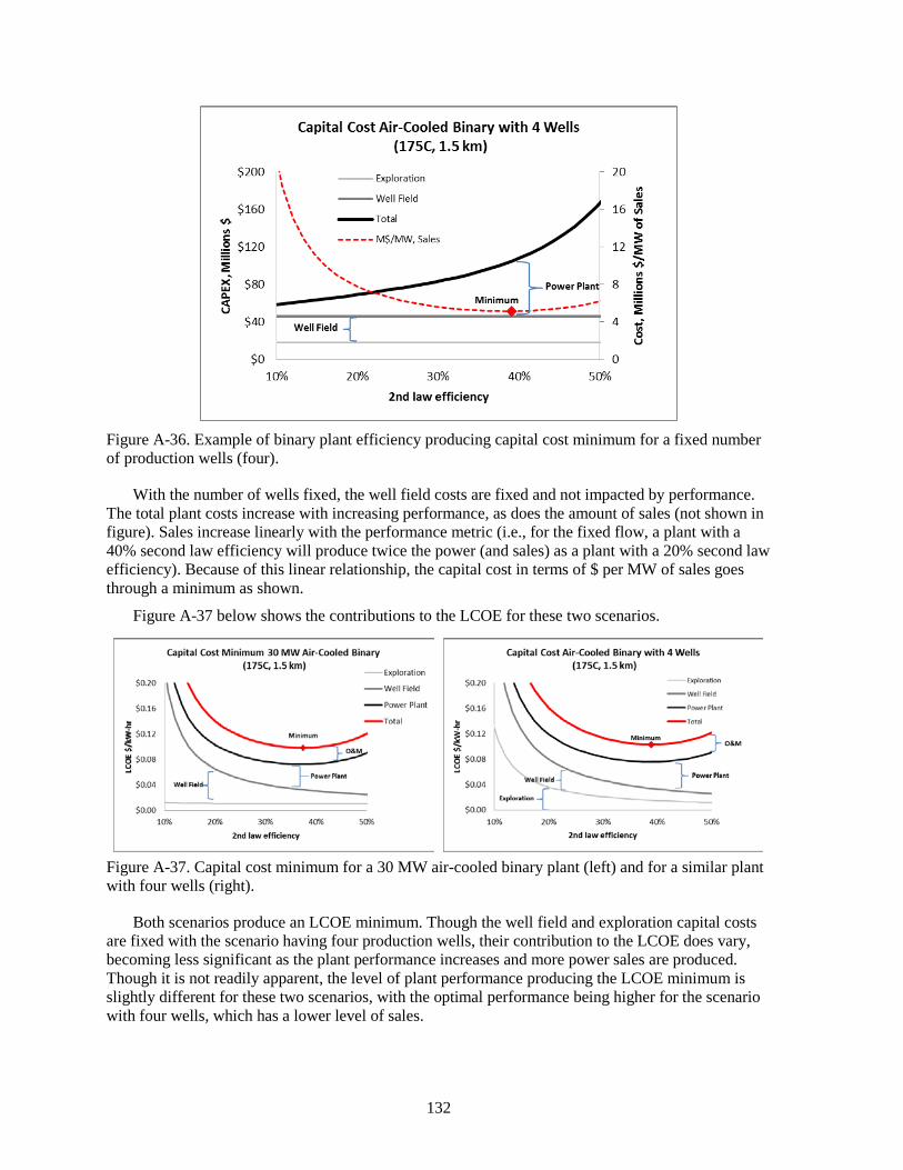
132

Figure A-36. Example of binary plant efficiency producing capital cost minimum for a fixed number of production wells (four).

With the number of wells fixed, the well field costs are fixed and not impacted by performance. The total plant costs increase with increasing performance, as does the amount of sales (not shown in figure). Sales increase linearly with the performance metric (i.e., for the fixed flow, a plant with a 40% second law efficiency will produce twice the power (and sales) as a plant with a 20% second law efficiency). Because of this linear relationship, the capital cost in terms of $ per MW of sales goes through a minimum as shown.

Figure A-37 below shows the contributions to the LCOE for these two scenarios.

Figure A-37. Capital cost minimum for a 30 MW air-cooled binary plant (left) and for a similar plant with four wells (right).

Both scenarios produce an LCOE minimum. Though the well field and exploration capital costs are fixed with the scenario having four production wells, their contribution to the LCOE does vary, becoming less significant as the plant performance increases and more power sales are produced. Though it is not readily apparent, the level of plant performance producing the LCOE minimum is slightly different for these two scenarios, with the optimal performance being higher for the scenario with four wells, which has a lower level of sales.

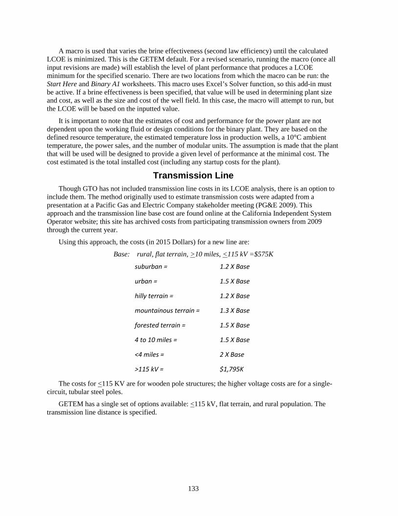
133

A macro is used that varies the brine effectiveness (second law efficiency) until the calculated LCOE is minimized. This is the GETEM default. For a revised scenario, running the macro (once all input revisions are made) will establish the level of plant performance that produces a LCOE minimum for the specified scenario. There are two locations from which the macro can be run: the Start Here and Binary A1 worksheets. This macro uses Excel’s Solver function, so this add-in must be active. If a brine effectiveness is been specified, that value will be used in determining plant size and cost, as well as the size and cost of the well field. In this case, the macro will attempt to run, but the LCOE will be based on the inputted value.

It is important to note that the estimates of cost and performance for the power plant are not dependent upon the working fluid or design conditions for the binary plant. They are based on the defined resource temperature, the estimated temperature loss in production wells, a 10°C ambient temperature, the power sales, and the number of modular units. The assumption is made that the plant that will be used will be designed to provide a given level of performance at the minimal cost. The cost estimated is the total installed cost (including any startup costs for the plant).

Transmission Line Though GTO has not included transmission line costs in its LCOE analysis, there is an option to

include them. The method originally used to estimate transmission costs were adapted from a presentation at a Pacific Gas and Electric Company stakeholder meeting (PG&E 2009). This approach and the transmission line base cost are found online at the California Independent System Operator website; this site has archived costs from participating transmission owners from 2009 through the current year.

Using this approach, the costs (in 2015 Dollars) for a new line are:

Base: rural, flat terrain, >10 miles, <115 kV = $575K

suburban = 1.2 X Base

urban = 1.5 X Base

hilly terrain = 1.2 X Base

mountainous terrain = 1.3 X Base

forested terrain = 1.5 X Base

4 to 10 miles = 1.5 X Base

<4 miles = 2 X Base

>115 kV = $1,795K

The costs for <115 KV are for wooden pole structures; the higher voltage costs are for a single-circuit, tubular steel poles.

GETEM has a single set of options available: <115 kV, flat terrain, and rural population. The transmission line distance is specified.

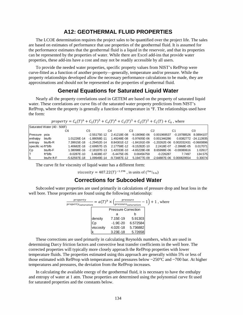
134

A12: GEOTHERMAL FLUID PROPERTIES The LCOE determination requires the project sales to be quantified over the project life. The sales

are based on estimates of performance that use properties of the geothermal fluid. It is assumed for the performance estimates that the geothermal fluid is a liquid in the reservoir, and that its properties can be represented by the properties of water. While there are Excel add-ins that provide water properties, these add-ins have a cost and may not be readily accessible by all users.

To provide the needed water properties, specific property values from NIST’s RefProp were curve-fitted as a function of another property—generally, temperature and/or pressure. While the property relationships developed allow the necessary performance calculations to be made, they are approximations and should not be represented as the properties of geothermal fluid.

General Equations for Saturated Liquid Water Nearly all the property correlations used in GETEM are based on the property of saturated liquid

water. These correlations are curve fits of the saturated water property predictions from NIST’s RefProp, where the property is generally a function of temperature in °F. The relationships used have the form:

𝑃𝑃𝑃𝑃𝑃𝑃𝑃𝑃𝑃𝑃𝑃𝑃𝑃𝑃𝑐𝑐 = 𝐿𝐿6(𝑇𝑇)6 + 𝐿𝐿5(𝑇𝑇)5 + 𝐿𝐿4(𝑇𝑇)4 + 𝐿𝐿3(𝑇𝑇)3 + 𝐿𝐿2(𝑇𝑇)2 + 𝐿𝐿1(𝑇𝑇) + 𝐿𝐿0 , where

The curve fit for viscosity of liquid water has a different form:

𝑙𝑙𝑃𝑃𝑆𝑆𝑃𝑃𝑃𝑃𝑆𝑆𝑃𝑃𝑃𝑃𝑐𝑐 = 407.22(𝑇𝑇)−1.194 , in units of (1bm/ft-hr)

Corrections for Subcooled Water Subcooled water properties are used primarily in calculations of pressure drop and heat loss in the

well bore. Those properties are found using the following relationship: 𝑝𝑝𝑝𝑝𝑔𝑔𝑝𝑝𝑛𝑛𝑝𝑝𝑛𝑛𝑎𝑎

𝑝𝑝𝑝𝑝𝑔𝑔𝑝𝑝𝑛𝑛𝑝𝑝𝑛𝑛𝑎𝑎𝑠𝑠𝑠𝑠𝑠𝑠𝑜𝑜𝑟𝑟𝑠𝑠𝑠𝑠𝑖𝑖𝑜𝑜𝑖𝑖= 𝑆𝑆(𝑇𝑇)𝑏𝑏 × � 𝑝𝑝𝑝𝑝𝑛𝑛𝑑𝑑𝑑𝑑𝑓𝑓𝑝𝑝𝑛𝑛

𝑝𝑝𝑝𝑝𝑛𝑛𝑑𝑑𝑑𝑑𝑓𝑓𝑝𝑝𝑛𝑛𝑠𝑠𝑠𝑠𝑠𝑠𝑜𝑜𝑟𝑟𝑠𝑠𝑠𝑠𝑖𝑖𝑜𝑜𝑖𝑖− 1� + 1 , where

These corrections are used primarily in calculating Reynolds numbers, which are used in

determining Darcy friction factors and convective heat transfer coefficients in the well bore. The corrected properties will typically more closely approach the RefProp properties with lower temperature fluids. The properties estimated using this approach are generally within 5% or less of those estimated with RefProp with temperatures and pressures below ~250°C and ~700 bar. At higher temperatures and pressures, the deviation from the RefProp increases.

In calculating the available energy of the geothermal fluid, it is necessary to have the enthalpy and entropy of water at 1 atm. Those properties are determined using the polynomial curve fit used for saturated properties and the constants below.

Saturated Water (40 - 500F)C6 C5 C4 C3 C2 C1 C0

Pressure psia -2.55175E-12 2.41218E-08 -9.19096E-06 0.001969537 -0.19788526 8.0894107enthalpy btu/lb 1.01226E-14 -1.88058E-11 1.49248E-08 -5.97605E-06 0.001346286 0.8382772 -24.113935entropy btu/lb-R 7.39915E-18 -1.29452E-14 8.84301E-12 -1.84191E-09 -1.20262E-06 0.002032431 -0.0600896specific vo ft 3/lb 1.40682E-18 -2.69957E-15 2.17758E-12 -9.15282E-10 2.2418E-07 -2.3968E-05 0.017071Cp btu/lb-F 1.38098E-16 -2.18187E-13 1.42033E-10 -4.65228E-08 8.65998E-06 -0.00080616 1.02617T ft 3/lb -9.0287E-10 3.4638E-07 -5.4475E-05 0.00456759 -0.226287 7.7497 134.575k btu/hr-ft-F -5.62597E-18 1.09949E-14 -9.73487E-12 5.19477E-09 -2.64887E-06 0.000829554 0.30074

Pressure Correctiona b

density 7.15E-19 5.91303Cp -1.9E-20 6.572584viscosity 4.02E-18 5.736882k 3.23E-18 5.72658

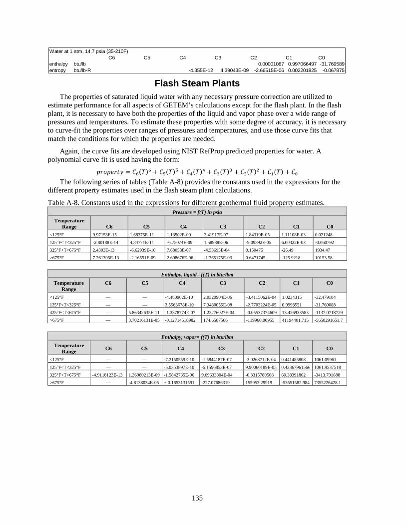
135

Flash Steam Plants The properties of saturated liquid water with any necessary pressure correction are utilized to

estimate performance for all aspects of GETEM’s calculations except for the flash plant. In the flash plant, it is necessary to have both the properties of the liquid and vapor phase over a wide range of pressures and temperatures. To estimate these properties with some degree of accuracy, it is necessary to curve-fit the properties over ranges of pressures and temperatures, and use those curve fits that match the conditions for which the properties are needed.

Again, the curve fits are developed using NIST RefProp predicted properties for water. A polynomial curve fit is used having the form:

𝑃𝑃𝑃𝑃𝑃𝑃𝑃𝑃𝑃𝑃𝑃𝑃𝑃𝑃𝑐𝑐 = 𝐿𝐿6(𝑇𝑇)6 + 𝐿𝐿5(𝑇𝑇)5 + 𝐿𝐿4(𝑇𝑇)4 + 𝐿𝐿3(𝑇𝑇)3 + 𝐿𝐿2(𝑇𝑇)2 + 𝐿𝐿1(𝑇𝑇) + 𝐿𝐿0 The following series of tables (Table A-8) provides the constants used in the expressions for the

different property estimates used in the flash steam plant calculations.

Table A-8. Constants used in the expressions for different geothermal fluid property estimates. Pressure = f(T) in psia

Temperature Range C6 C5 C4 C3 C2 C1 C0

<125°F 9.97153E-15 1.68375E-11 1.13502E-09 3.41917E-07 1.84319E-05 1.11108E-03 0.021248

125°F<T<325°F -2.80188E-14 4.34771E-11 -6.75074E-09 1.58988E-06 -9.09892E-05 6.00322E-03 -0.060792

325°F<T<675°F 2.4303E-13 -6.62939E-10 7.68058E-07 -4.53695E-04 0.150475 -26.49 1934.47

>675°F 7.261395E-13 -2.16551E-09 2.698676E-06 -1.765175E-03 0.6471745 -125.9218 10153.58

Enthalpy, liquid= f(T) in btu/lbm

Temperature Range

C6 C5 C4 C3 C2 C1 C0

<125°F — — -4.480902E-10 2.0320904E-06 -3.4115062E-04 1.0234315 -32.479184

125°F<T<325°F — — 2.5563678E-10 7.3480055E-08 -2.7703224E-05 0.9998551 -31.760088

325°F<T<675°F — 5.86342635E-11 -1.3378774E-07 1.22276027E-04 -0.05537374609 13.426933583 -1137.0718729

>675°F — 3.70216131E-05 -0.12714518982 174.6587566 -119960.00955 41194401.715 -5658291651.7

Enthalpy, vapor= f(T) in btu/lbm

Temperature Range C6 C5 C4 C3 C2 C1 C0

<125°F — — -7.2150559E-10 -1.5844187E-07 -3.0268712E-04 0.441485808 1061.09961

125°F<T<325°F — — -5.0353897E-10 -5.1596853E-07 9.90060189E-05 0.42367961566 1061.9537518

325°F<T<675°F -4.9118123E-13 1.36980213E-09 -1.5842735E-06 9.69633804E-04 -0.3315780568 60.38391862 -3413.791688

>675°F — -4.8138034E-05 + 0.1653131591 -227.07686319 155953.29919 -53551582.984 7355226428.1

Water at 1 atm, 14.7 psia (35-210F)C6 C5 C4 C3 C2 C1 C0

enthalpy btu/lb 0.00001087 0.997066497 -31.769589entropy btu/lb-R -4.355E-12 4.39043E-09 -2.66515E-06 0.002201825 -0.067875

136

Entropy, liquid= f(T) in btu/lbm-°R Temperature

Range C6 C5 C4 C3 C2 C1 C0 <125°F — — — 2.964634E-09 -2.499642E-06 0.002195168 -0.06778459

125°F<T<325°F — — -9.593628E-13 2.223552E-09 -2.16312E-06 0.00215356 -0.06615222

325°F<T<675°F 5.297508E-16 -1.495185E-12 1.739088E-09 -1.064881E-06 3.612208E-04 -0.06296176 4.729245

>675°F 1.100136E-10 -4.450574E-07 7.501037E-04 -0.674174 340.7939 -91866.44 10317090

Entropy, vapor= f(T) in btu/lbm-°R

Temperature Range C6 C5 C4 C3 C2 C1 C0

<125°F — — 2.38219E-11 -2.213415E-08 0.00001113945 -0.004205795 2.312154

125°F<T<325°F — — 8.392618E-12 -1.361597E-08 9.334758E-06 -0.004032959 2.305898

325°F<T<675°F -8.283605E-16 2.333203E-12 -2.708314E-09 1.65401E-06 -5.589582E-04 0.09784205 -5.19791

>675°F -1.41418E-10 5.720121E-07 -9.639254E-04 0.8662219 -437.8104 118002.2 -13250460

Specific volume, vapor= f(T) in ft3/lbm

Temperature Range C6 C5 C4 C3 C2 C1 C0

<125°F 4.5215227E-09 -2.7557218E-06 0.00071596466 - 0.1033793 8.9931223 -464.41472 11678.605

125°F<T<325°F 1.1909478E-11 -1.8270648E-08 1.1692082E-05 -4.0132715E-03 0.78482148 - 83.834081 3890.919

325°F<T<675°F 8.187709E-15 -2.7284644E-11 3.7948334E-08 -2.8277928E-05 0.011958041 -2.7389634 268.32894

>675°F — — -8.7731388E-09 2.3582903E-05 -0.023769687 10.645163 -1786.8983

Temperature= f(P,psia) in °F

Pressure Range C6 C5 C4 C3 C2 C1 C0 <2 psia -7.18640668 63.30476138 -222.3098297 400.5726943 -403.5629735 255.8563258 14.788

2<P<20 psia -1.2178122E-05 9.43580389E-04 -0.0297343763 0.4946879155 -4.801670172 31.49104908 78.872

20<P<200 psia -1.287831E-11 1.0530967E-08 -3.4988476E-06 6.12922921E-04 -0.062604067 4.368874775 161.409

200<P<1000 psia -4.3371352E-16 1.88671656E-12 -3.4275245E-09 3.40481648E-06 -2.0724713E-03 0.9305613192 256.297

>1000 psia -3.2288676E-19 4.5896969E-15 -2.7823504E-11 9.44074178E-08 -2.0256474E-04 0.333459111 342.906

In relating the specific volume of saturated water vapor to pressure, two different correlations are

used (dependent upon pressure). For higher-pressure vapors, the following is used:

specific volumevapor = C6(P)6 + C5(P)5 + C4(P)4 + C3(P)3 + C2(P)2 + C1(P) + C0 , where Specific volume, vapor= f(P,psia) in ft3/lbm

Pressure Range C6 C5 C4 C3 C2 C1 C0 200<P<1000 psia 4.07239263E-17 -1.7199693E-13 2.98853804E-10 -2.7579166E-07 1.45475053E-04 -0.0438346609 7.01332874

>1000 psia -8.2949288E-21 8.10943127E-17 -2.8059086E-13 3.05379716E-10 4.5750427E-07 -0.00155021959 1.44118272

At lower pressures, the following is used:

𝑆𝑆𝑃𝑃𝑃𝑃𝑃𝑃𝑃𝑃𝑓𝑓𝑃𝑃𝑃𝑃 𝑙𝑙𝑃𝑃𝑆𝑆𝑃𝑃𝑃𝑃𝑃𝑃𝑎𝑎𝑝𝑝𝑝𝑝𝑔𝑔𝑝𝑝 = 𝑆𝑆(𝑃𝑃)𝑏𝑏 , where Specific volume, vapor= f(P,psia) in ft3/lbm

Pressure Range a b <2 psia 333.81229512 -0.94402159016 2<P<20 psia 332.15976378 -0.93664745606 20<P<200 psia -1.287831E-11 -0.94294510344

137

These properties are the basis for determining the flash plant performance and equipment sizes used to determine the plant cost. The flash plant performance is the basis for sizing the well field, or for establishing the amount of power sales from a fixed number of wells for a defined resource scenario.

Impact of GETEM Properties on LCOE A recent version of GETEM was modified to determine all fluid properties using a RefProp

add-in to Excel instead of the different correlations described. Two hydrothermal resource scenarios were considered, one using a binary plant and the other a flash steam plant.

The resource defined that utilized the binary plant was at 175°C and a depth of 1.5 km. The resource using the flash steam plant was at 250°C and 2.5 km. The binary plant had sales of 30 MW; the flash plant had sales of 40 MW. The following summarizes the impact of using the correlations in GETEM to estimate water properties.

Table A-9. The impact of using GETEM’s correlations for water properties on important project metrics.

Parameter

BINARY FLASH STEAM GETEM

Properties RefProp GETEM

Properties RefProp Sales (MW) 30 30 40 40 Plant size (MW) 34.373 34.301 41.808 41.813 Number of successful production wells

6.19 6.17 4.80 4.80

Total GF flow (kg/s) 618.7 617.4 384.1 384.0 Temperature loss in well (°C)

1.35 1.35 3.37 3.37

Total overnight cost (million $)

$162.724 $162.373 $152.214 $152.245

PV of power over life (MW · hrs)

2,726,853 2,727,773 3,622,622 3,622,078

LCOE ($/kW · h) $0.0984 $0.0982 $0.0685 $0.0686

Comparing results for the two resource scenarios indicate that, while the GETEM properties are only approximations, their use did not substantially impact the performance or costs obtained.

Silica Temperature Limit It is assumed that a minimum temperature limit is placed on the geothermal fluid to prevent

mineral precipitation—specifically, the precipitation of amorphous silica. This temperature limit is used when setting operating constraints on flash pressures for steam plants, and, if imposed, can impact the calculation of the injection pumping power. Though it is not specifically applied in any of the binary plant calculations in GETEM, it was imposed during the Aspen modeling that is the basis for the cost and performance calculations in GETEM. With binary plants, it may be imposed when estimating the temperature of the injected brine.

138

In early versions of GETEM, the temperature constraint was determined using expressions for the solubility temperature of amorphous silica based on correlations reported by Fournier (1981). These relationships were used to relate the solubility temperature of amorphous silica to a resource temperature, assuming that the silica went into solution either as quartz or as chalcedony.

quartz: 𝑇𝑇𝑝𝑝𝑝𝑝𝑔𝑔𝑝𝑝𝑝𝑝ℎ𝑔𝑔𝑓𝑓𝑑𝑑 𝑑𝑑𝑓𝑓𝑓𝑓𝑓𝑓𝑎𝑎𝑝𝑝 = 0.000658�𝑇𝑇𝑝𝑝𝑛𝑛𝑑𝑑𝑔𝑔𝑓𝑓𝑝𝑝𝑎𝑎𝑛𝑛2� + 0.712233(𝑇𝑇𝑝𝑝𝑛𝑛𝑑𝑑𝑔𝑔𝑓𝑓𝑝𝑝𝑎𝑎𝑛𝑛) − 93.2874 chalcedony: 𝑇𝑇𝑝𝑝𝑝𝑝𝑔𝑔𝑝𝑝𝑝𝑝ℎ𝑔𝑔𝑓𝑓𝑑𝑑 𝑑𝑑𝑓𝑓𝑓𝑓𝑓𝑓𝑎𝑎𝑝𝑝 = 0.000148�𝑇𝑇𝑝𝑝𝑛𝑛𝑑𝑑𝑔𝑔𝑓𝑓𝑝𝑝𝑎𝑎𝑛𝑛2� + 0.774255(𝑇𝑇𝑝𝑝𝑛𝑛𝑑𝑑𝑔𝑔𝑓𝑓𝑝𝑝𝑎𝑎𝑛𝑛) − 70.4349

In both of these expressions, temperatures (T) are in °C. In GETEM, the correlation based on chalcedony solubility was used for resource temperatures below 180°C. The correlation based on quartz solubility was used for resource temperatures of 180°C and higher.

These expressions were used in the modeling of the binary plants, the results of which are the basis of GETEM’s estimates for these air-cooled plants. Their use produced a discontinuity in the limit as shown in Figure A-38 below.

Figure A-38. Amorphous silica solubility temperatures used in early versions of GETEM.

The discontinuity that occurs when switching between the two solubility curves produced similar discontinuities in GETEM’s calculations.

To resolve this, the approach for characterizing this temperature limit was revised. Correlations from Gunnarsson and Arnorsson (2000) were used to develop the following expressions for the solubility of quartz and amorphous silica. 𝑆𝑆𝑃𝑃𝑂𝑂2𝑟𝑟𝑓𝑓𝑝𝑝𝑝𝑝𝑛𝑛𝑞𝑞 = −1.334837 × 10−7�𝑇𝑇𝐹𝐹4� + 7.065845 × 10−5�𝑇𝑇𝐹𝐹3� + 3.62948 × 10−3�𝑇𝑇𝐹𝐹2� + 0.367242(𝑇𝑇𝐹𝐹) + 4.2059

𝑇𝑇𝑟𝑟𝑃𝑃𝑝𝑝𝑔𝑔𝑝𝑝𝑝𝑝ℎ𝑔𝑔𝑓𝑓𝑑𝑑 𝑑𝑑𝑓𝑓𝑓𝑓𝑓𝑓𝑎𝑎𝑝𝑝 = 2.49634 × 10−11 �𝑆𝑆𝑃𝑃𝑂𝑂2𝑟𝑟𝑓𝑓𝑝𝑝𝑝𝑝𝑛𝑛𝑞𝑞4� − 4.25191 × 10−9 �𝑆𝑆𝑃𝑃𝑂𝑂2𝑟𝑟𝑓𝑓𝑝𝑝𝑝𝑝𝑛𝑛𝑞𝑞

3� − 1.19669 × 10−3 �𝑆𝑆𝑃𝑃𝑂𝑂2𝑟𝑟𝑓𝑓𝑝𝑝𝑝𝑝𝑛𝑛𝑞𝑞2�

+ 0.307616 �𝑆𝑆𝑃𝑃𝑂𝑂2𝑟𝑟𝑓𝑓𝑝𝑝𝑝𝑝𝑛𝑛𝑞𝑞� − 0.2944

In these relationships, temperature (T) is in °C. The amount of silica (SiO2 quartz) is the silica concentration in solution (ppm). The correlations upon which these relationships were derived were determined for a temperature range from 8° to 310°C. Use of these relationships produce a single curve for the solubility of amorphous silica without discontinuity as shown in Figure A-39 below.

139

Figure A-39. Current and prior GETEM estimates of amorphous silica solubility temperatures.

The calculations that are made in GETEM are intended to be representative of geothermal power production. To do so, it is necessary to approximate the properties of the geothermal fluid. These methods do not produce results that deviate significantly from those obtained when using recognized software to generate the properties needed. Even though the results are favorable for the two resource scenarios considered, there will be instances in which these methods do no work. Those are likely to be higher-temperature resources, resources with higher reservoir pressures, and/or resources having high levels of dissolved solids.

140

A13: PRODUCER PRICE INDEXES The costs used to determine an LCOE are derived from several sources, each of which is based on

a specific year. In order to utilize these costs, as well as to allow GETEM to estimate costs for a specified year, a cost index is applied to GETEM’s base cost estimated. The cost indices used are the Producer Price Indexes (PPIs) obtained from the U.S. Bureau of Labor Statistics. In determining a cost in a specified year, a designated PPI is multiplied by the estimate developed in GETEM.

𝑆𝑆𝑃𝑃𝑃𝑃𝑃𝑃𝑃𝑃𝑓𝑓𝑃𝑃𝑃𝑃𝑑𝑑 𝑐𝑐𝑃𝑃 𝑃𝑃𝑃𝑃𝑆𝑆𝑃𝑃𝑛𝑛 = 𝑃𝑃𝑃𝑃𝐼𝐼𝑛𝑛 × 𝐺𝐺𝐿𝐿𝑇𝑇𝐿𝐿𝑀𝑀 𝑃𝑃𝑆𝑆𝑃𝑃𝑃𝑃𝑃𝑃𝑆𝑆𝑃𝑃𝑃𝑃𝑑𝑑 𝑃𝑃𝑃𝑃𝑆𝑆𝑃𝑃𝑏𝑏𝑝𝑝𝑑𝑑𝑛𝑛 The PPIs used are tabulated below in Table A-10, along with the GETEM estimates/default

inputs to which they are applied.

Table A-10. Producer Price Index categories with reference year and description of application to default costs.

PPI Category Applied to Default Costs Reference

Year Comment Manufacturing Labor

Applied to operation and maintenance labor; used in a discontinued method of estimating binary plant equipment costs. 2002

Construction Labor Applied to estimates of labor contribution to direct construction multiplier for both binary and flash steam power plants. 2002

Engineering Applied to default well testing costs; used in a discontinued approach for determining indirect costs for plant construction. 2002

Steel Applied to estimates of steel contribution to direct construction multiplier for both binary and flash steam power plants (includes piping).

2002

Pipe Applied to estimates for field gathering system and production pump casing; used as indicator for increases in casing cost in internal well cost model (not reported).

2002

Electrical (average used) PPI for process equipment used. 2002 No longer

used Turbine-Generator Applied to power plant turbine-generator cost estimate. 2002 Heat Exchangers Applied to all estimated heat exchanger costs. 2002

Pumps Applied to all power plant cost estimates; applied to injection pump and production pump estimates. 2002

Process Equipment (average used)

Binary plants: applied to estimates of both the “other” and construction materials contributions to direct construction multiplier. Flash plants: same as binary plus applied to flash vessels, cooling tower, NCG removal, and H2S abatement systems.

2002

Oil & Gas Well Adjust cost for small-diameter exploration drilling; adjust default costs for well drilling costs; applied to material elements of internal well cost model (not reported).

2010

Drilling Services Applied to estimates for pump installation and well stimulation default cost; applied to services in internal well cost model (not reported). 2010

Cement Applied to cement costs in internal well cost model (not reported). 2010 Legal Services Applied to permitting costs. 2012

Oil & Gas Support Applied to non-drilling exploration costs; applied to “other” costs determined in internal well cost model (not reported). 2010

Directional Drilling Applied to directional drilling costs determined in internal well cost model (not reported). 2010

Chemicals Applied to treatment costs for cooling tower and geothermal fluid. 2007 Petroleum Products Applied to lubrication oil used with line-shaft pumps. 2001

The PPIs are applied to the model default costs. If a cost input is revised, the PPI is not applied. It is assumed that the inputted value is current for the year being evaluated. If input is revised that is not a cost, the PPIs are applied to the cost estimated using the revised input.

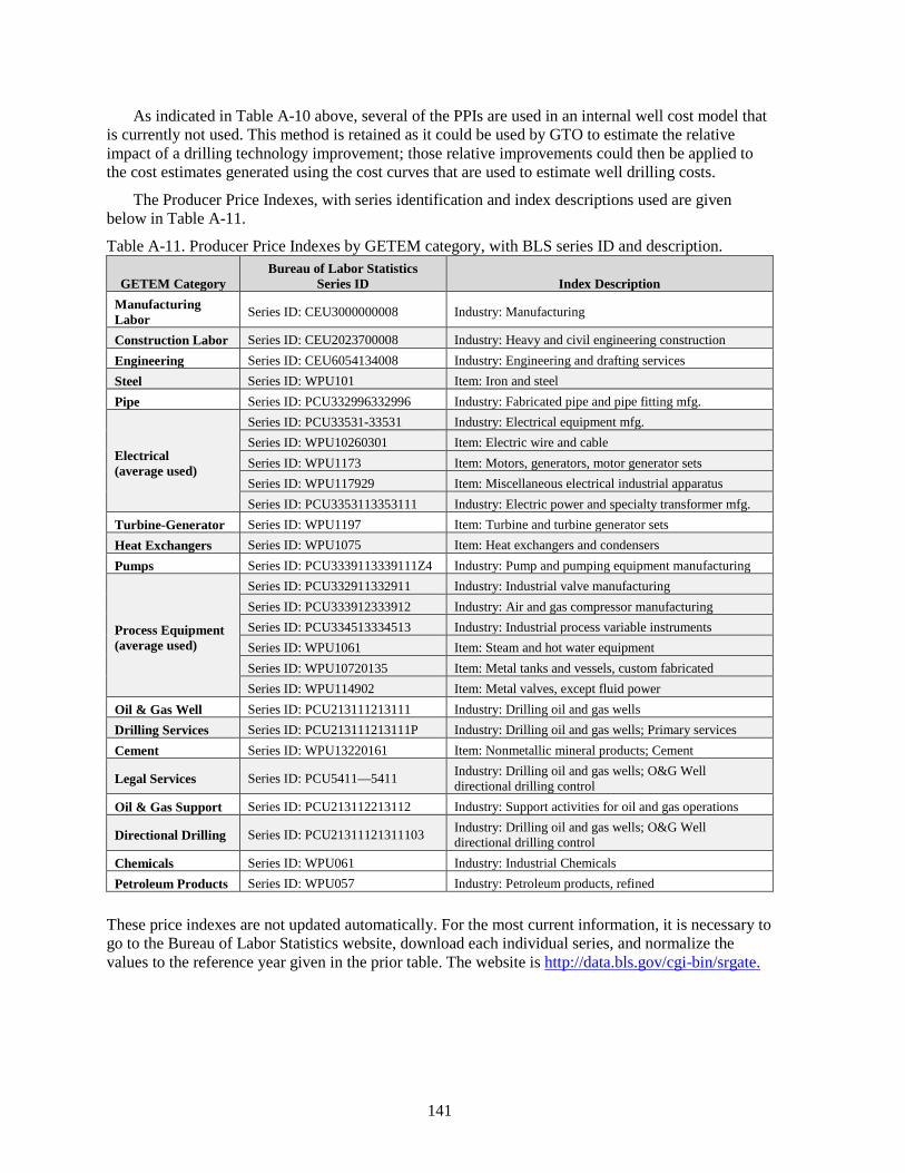
141

As indicated in Table A-10 above, several of the PPIs are used in an internal well cost model that is currently not used. This method is retained as it could be used by GTO to estimate the relative impact of a drilling technology improvement; those relative improvements could then be applied to the cost estimates generated using the cost curves that are used to estimate well drilling costs.

The Producer Price Indexes, with series identification and index descriptions used are given below in Table A-11.

Table A-11. Producer Price Indexes by GETEM category, with BLS series ID and description.

GETEM Category Bureau of Labor Statistics

Series ID Index Description Manufacturing Labor Series ID: CEU3000000008 Industry: Manufacturing

Construction Labor Series ID: CEU2023700008 Industry: Heavy and civil engineering construction Engineering Series ID: CEU6054134008 Industry: Engineering and drafting services Steel Series ID: WPU101 Item: Iron and steel Pipe Series ID: PCU332996332996 Industry: Fabricated pipe and pipe fitting mfg.

Electrical (average used)

Series ID: PCU33531-33531 Industry: Electrical equipment mfg. Series ID: WPU10260301 Item: Electric wire and cable Series ID: WPU1173 Item: Motors, generators, motor generator sets Series ID: WPU117929 Item: Miscellaneous electrical industrial apparatus Series ID: PCU3353113353111 Industry: Electric power and specialty transformer mfg.

Turbine-Generator Series ID: WPU1197 Item: Turbine and turbine generator sets Heat Exchangers Series ID: WPU1075 Item: Heat exchangers and condensers Pumps Series ID: PCU3339113339111Z4 Industry: Pump and pumping equipment manufacturing

Process Equipment (average used)

Series ID: PCU332911332911 Industry: Industrial valve manufacturing Series ID: PCU333912333912 Industry: Air and gas compressor manufacturing Series ID: PCU334513334513 Industry: Industrial process variable instruments Series ID: WPU1061 Item: Steam and hot water equipment Series ID: WPU10720135 Item: Metal tanks and vessels, custom fabricated Series ID: WPU114902 Item: Metal valves, except fluid power

Oil & Gas Well Series ID: PCU213111213111 Industry: Drilling oil and gas wells Drilling Services Series ID: PCU213111213111P Industry: Drilling oil and gas wells; Primary services Cement Series ID: WPU13220161 Item: Nonmetallic mineral products; Cement

Legal Services Series ID: PCU5411—5411 Industry: Drilling oil and gas wells; O&G Well directional drilling control

Oil & Gas Support Series ID: PCU213112213112 Industry: Support activities for oil and gas operations

Directional Drilling Series ID: PCU21311121311103 Industry: Drilling oil and gas wells; O&G Well directional drilling control

Chemicals Series ID: WPU061 Industry: Industrial Chemicals Petroleum Products Series ID: WPU057 Industry: Petroleum products, refined

These price indexes are not updated automatically. For the most current information, it is necessary to go to the Bureau of Labor Statistics website, download each individual series, and normalize the values to the reference year given in the prior table. The website is http://data.bls.gov/cgi-bin/srgate.

142

A14: ERROR AND WARNINGS The Error-Warnings worksheet lists potential issues with the input provided. When there is a

potential issue, “Error/Warnings” will appear at the top of the worksheets where input is provided. This is a link to the Error-Warnings worksheet. The number following this link is the count of the number of potential issues found. When there is an issue, a message will be displayed on the Error-Warnings worksheet describing the issue. Adjacent to the message is a link to the location where the input is being questioned.

The following is a list of the current messages followed by possible responses to resolve the issues:

The number of production wells inputted is less than the number of successful production wells drilled during Exploration.

This message occurs if the number of production wells specified is less than the number of successful production wells drilled during exploration. Correct this by changing the number of production wells that the project evaluation is being based upon, or by changing the number of successful wells drilled during exploration. It is also possible to clear the message by reducing the productivity of the production wells (flow rate and/or productivity index) or using a less efficient power plant.

The model cannot calculate using a defined Resource Temperature that exceeds the Critical Temperature of Water.

The properties used in GETEM to estimate performance are limited to temperatures below the critical temperature of water (374°C). The correlations used in GETEM provide reasonable approximations of water properties for temperatures up to ~300°C.

The resource depth exceeds the maximum for using the GETEM methodology for well cost.

GETEM’s cost correlations are developed from estimates for depths to 6 km.

The power sales specified requires fewer production wells than were successfully drilled during Exploration. Increase sales or reduce the number of successful Exploration wells, the flow per well or the plant performance.

Increase sales or reduce the number of successful exploration wells. It is also possible to clear this by decreasing the well flow and/or plant performance. This message may accompany other messages.

The duration of pre-startup activities exceeds that allowed in GETEM when using the EERE/DCF methodology.

Reduce the duration of one or more of the pre-operational activities. Up to 14 years total for these activities is allowed for the model.

Model cannot evaluate projects operating longer than 40 years.

This limitation on the project life is inherent to the model; it results from the method used to determine the power production as the resource temperature declines with time.

When using Fixed Charge Rate Method, project life for all cases = 30 yr

This limitation is based on the default fixed charge rate used, which is based on the assumption of a 30-year life.

For the scenario defined, the plant output will go to 0 before the end of project life. Clear the warning by either defining more resource potential

143

found during Exploration, reducing power sales, decreasing project life or decreasing temperature decline rate.

This message will occur when the specified annual temperature decline is sufficient that the predicted output goes to zero before the end of the stated project life. This can be cleared by reducing the temperature decline rate, the project life, or both. It can also be cleared by changing resource potential and power sales to allow for re-drilling the well field.

The plant net plant output exceeds the potential resource found.

This message is cleared by either reducing the level of sales or increasing the resource potential found at the developed site. When this message occurs, there will be no makeup drilling.

Recommend not Proportioning EGS Exploration Costs with Resource Potential Found.

This message is based on the premise that makeup drilling will be necessary with EGS.

No full-sized wells drilled during Exploration of Hydrothermal Greenfield Project.

To clear this message, either exploration drilling is included for the defined scenario, or the project type is changed to Field Expansion.

Exploration drilling is occurring at more sites than were examined during pre-drilling evaluation.

This message can appear when the down-select process for developing a project is used in the evaluation. Either increase the number of sites evaluated or reduce the number of sites with drilling.

Full-sized Exploration wells are drilled at more sites than have small-diameter well drilling.

This message can appear when the down-select process for developing a project is evaluated. Either increase the number of sites at which small-diameter wells are drilled or reduce the number of site where full-sized exploration wells are drilled.

No full-diameter wells are drilled during Exploration of ‘Greenfield’ project.

Exploration Wells for a Hydrothermal Resource are to be stimulated. If stimulation required, evaluate as EGS resource.

The successful Exploration wells for an EGS Resource are not being stimulated. If no Exploration stimulation is required, evaluate as a Hydrothermal Resource.

The default is that EGS resources are stimulated and that at least one well drilled during the exploration phase be successfully stimulated. If input for the hydrothermal resource indicates wells are stimulated during the exploration phase, the scenario should be defined as using an EGS resource.

Two successful full-size Exploration wells required for EGS.

This is based on the assumption that EGS requires demonstration of coupled production and injection wells to establish the commercial viability of the resource.

No stimulation failures for Exploration wells.

#Stimulations specified < #successful wells stimulated - Increase number of stimulations and/or revise well type stimulated.

144

These messages are may occur when evaluating EGS scenarios. The number of wells stimulated during exploration is based upon the number of successful wells drilled and the type of well stimulated. At least one well must be successfully stimulated.

The defined scenario has no injection wells being drilled.

Unless the project evaluated is for a Field Expansion, injection wells will be required.

Drilling Success Rate should be >0% and <=100%.

When wells are stimulated, unsuccessful wells are not used to supplement injection. This applied to Hydrothermal as well as EGS resources. If Hydrothermal resource, must indicate which well type is stimulated.

When wells are stimulated, failed wells are not used to supplement injection regardless of the resource type being evaluated. Because the default for hydrothermal resources is that no stimulation will occur, it is necessary to identify whether production wells, injection wells, or both well types are stimulated.

When failed wells are used to supplement injection, their relative productivity should be between 0 and 1.

If the productivity is one or greater, it is not likely the wells would be considered failures.

With pumping, the bottom hole pressure in the injection well is 50%+ higher than the estimated hydrostatic pressure. Consider reducing the flow rate per injection well, and/or increase the Injectivity Index.

The 50% value in this message is arbitrary, intended to provide warning that the pressures used may promote fracturing of the reservoir and/or seismic activity.

Need to use Larger Diameter production well size at the specified resource depth in order to allow for production pump with Binary plant. Minimum casing size 13-3/8 inch

This message occurs if a Smaller-Diameter well is specified with binary plant.

Stimulation has been specified with a Hydrothermal Resource scenario.

No stimulation specified with EGS Resource scenario.

These messages apply to the drilling phase. The default is that hydrothermal resources will not be stimulated, while EGS resources will be.

The stimulation success rates should be between 0 and 100%.

Pump efficiency should be >0% & <100%.

Specified success rates and efficiencies should be greater than zero. Specified efficiencies are less than 100 %. Specified success rates can be as high as, but should not exceed, 100%.

Cannot input pump depth with EGS resource - inputted value ignored & calculated pump depth is used if wells are pumped.

Inputting a pump depth with an EGS resource can produce circular reference.

The pump depth exceeds the depth of the resource/production well. The inputted depth needs to be reduced, if calculated, the well flow rate needs to be reduced, or productivity index increased.

145

When inputted pump depth less than calculated, it is probable that geofluid will flash before getting to binary plant heat exchangers. To decrease calculated depth, decrease well flow or increase Productivity Index.

The calculated pump depth is a function of a number of parameters; the well flow rate and productivity index that are specified are the major contributors to this depth. Decreasing flow rate or increasing reservoir hydraulic productivity will decrease the calculated pump depth.

Any input for water loss or water cost is ignored with Hydrothermal Resource scenarios using air-cooled binary plants.

Pump depth exceeds 2,000 ft limit for specified Lineshaft Pump. Change pump type, change inputted depth or reduce flow/increase productivity index.

Flashing may occur in Production Well or surface piping - OK with Flash Plant. If Binary, use pumped wells or revise inputted pump depth.

With inputted pump depth, flashing is predicted in Production Well or surface piping with a Binary Plant.

The geothermal pumping power exceeds the plant output – define a more efficient plant, decrease flow and/or increase Productivity/Injectivity Index.

If you input the O&M LCOE contribution, you must enter a value for the contributions from both the plant and well field.

Revised Binary Plant Performance exceeds that allowed in GETEM’s Cost Correlations.

GETEM’s correlations that relate binary cost to plant performance are based on estimated costs for a range of performance at each resource temperature evaluated. The value that is inputted is outside that performance range. GETEM will try to estimate a cost based on the value provided, but that estimate should be considered suspect.

The HP or Single Flash pressure is out of range - it exceeds the estimated wellhead pressure or is less than 1 atmosphere; production well needs to be pumped, the well flow rate reduced or flash pressure revised.

LP Flash pressure exceeds HP Flash Pressure - revise LP Flash pressure.

LP flash pressure is less than 1 atm - reduce well flow rate or use production pumps.

Pressure losses in the production well are only approximations once the geothermal fluid begins to flash. The warnings provided are to advise that there may be a problem with inputted values. GETEM uses the inputs provided for flash pressures (default or revised) and not estimated wellhead pressures.

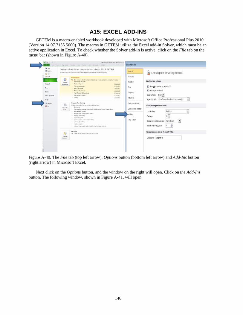
146

A15: EXCEL ADD-INS GETEM is a macro-enabled workbook developed with Microsoft Office Professional Plus 2010

(Version 14.07.7155.5000). The macros in GETEM utilize the Excel add-in Solver, which must be an active application in Excel. To check whether the Solver add-in is active, click on the File tab on the menu bar (shown in Figure A-40).

Figure A-40. The File tab (top left arrow), Options button (bottom left arrow) and Add-Ins button (right arrow) in Microsoft Excel.

Next click on the Options button, and the window on the right will open. Click on the Add-Ins button. The following window, shown in Figure A-41, will open.

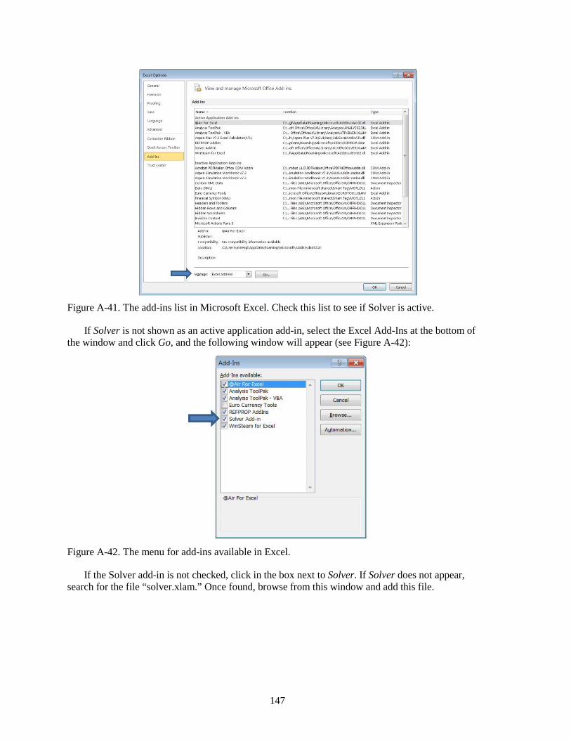
147

Figure A-41. The add-ins list in Microsoft Excel. Check this list to see if Solver is active.

If Solver is not shown as an active application add-in, select the Excel Add-Ins at the bottom of the window and click Go, and the following window will appear (see Figure A-42):

Figure A-42. The menu for add-ins available in Excel.

If the Solver add-in is not checked, click in the box next to Solver. If Solver does not appear, search for the file “solver.xlam.” Once found, browse from this window and add this file.

148

If Solver has been added and the macro works, click on the Developer tab on the menu bar, then on Visual Basic as shown in Figure A-43.

Figure A-43. The Developer tab (right arrow) and Visual Basic button (left arrow) in Microsoft Excel.

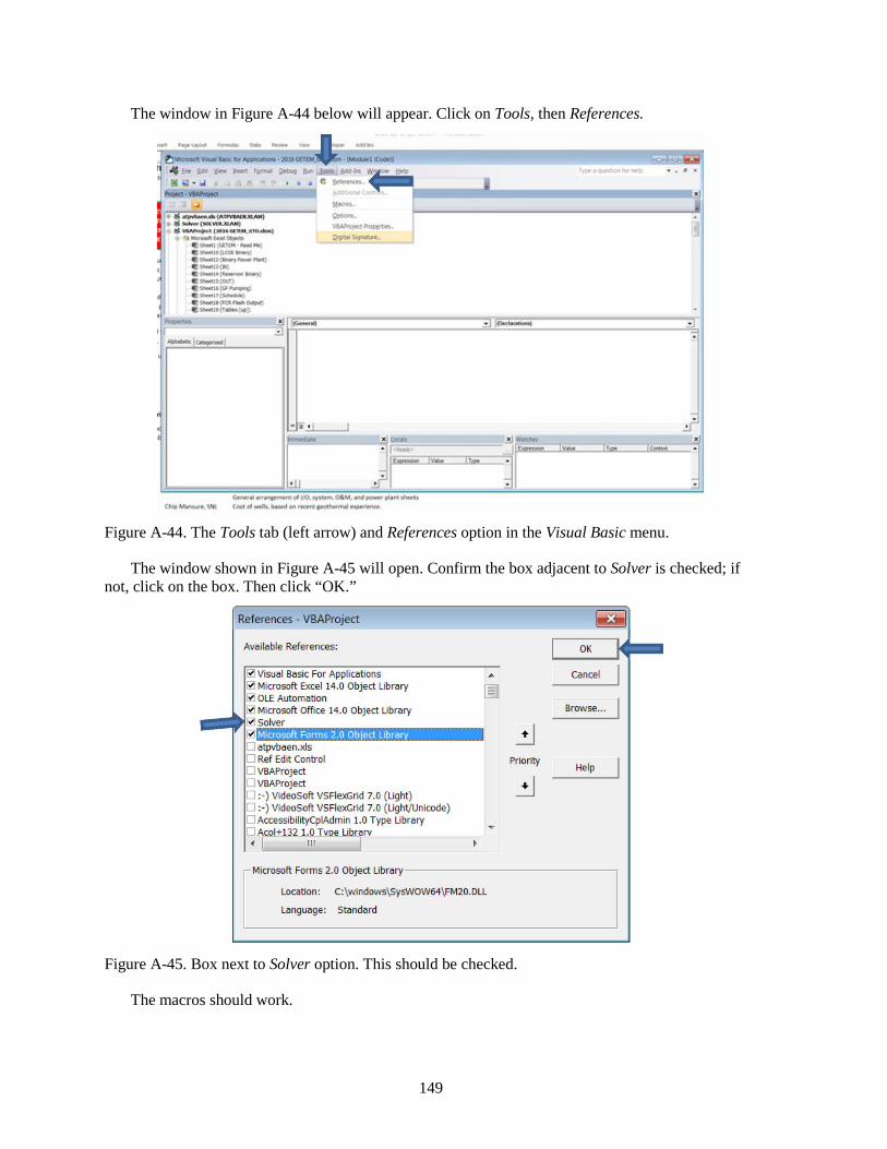
149

The window in Figure A-44 below will appear. Click on Tools, then References.

Figure A-44. The Tools tab (left arrow) and References option in the Visual Basic menu.

The window shown in Figure A-45 will open. Confirm the box adjacent to Solver is checked; if not, click on the box. Then click “OK.”

Figure A-45. Box next to Solver option. This should be checked.

The macros should work.

150

151

Appendix B

Information on GETEM’s Reservoir Inputs

152

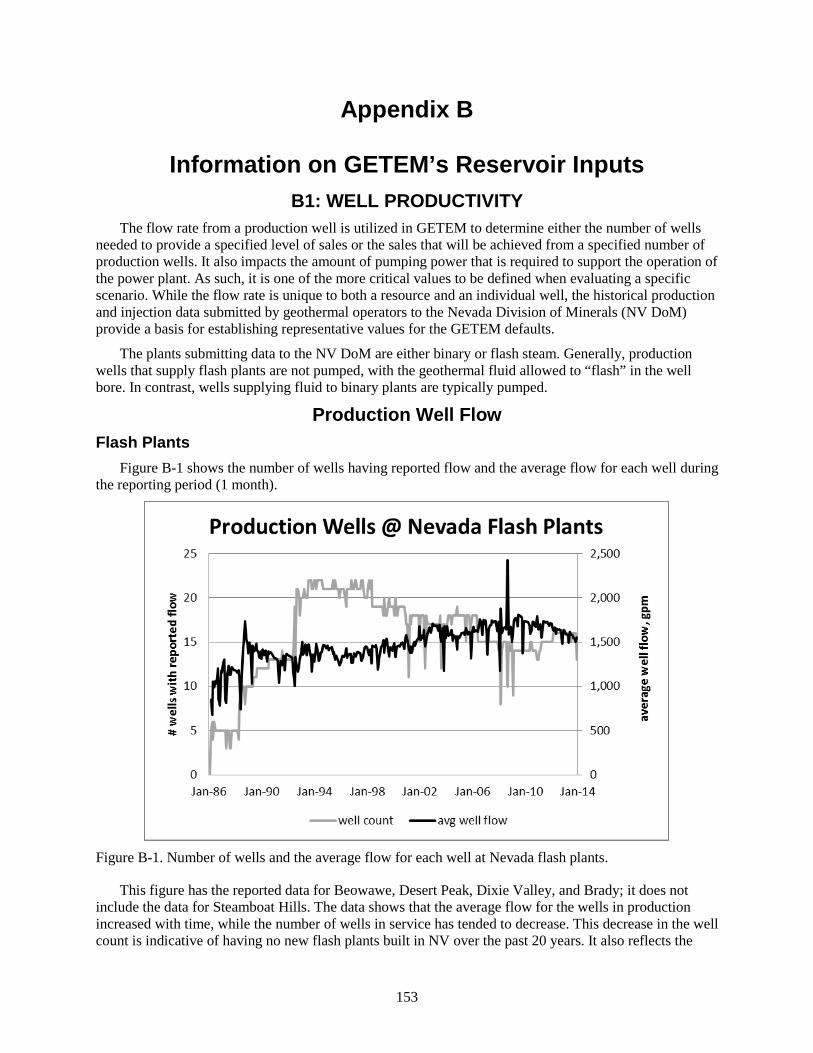
153

Appendix B

Information on GETEM’s Reservoir Inputs B1: WELL PRODUCTIVITY

The flow rate from a production well is utilized in GETEM to determine either the number of wells needed to provide a specified level of sales or the sales that will be achieved from a specified number of production wells. It also impacts the amount of pumping power that is required to support the operation of the power plant. As such, it is one of the more critical values to be defined when evaluating a specific scenario. While the flow rate is unique to both a resource and an individual well, the historical production and injection data submitted by geothermal operators to the Nevada Division of Minerals (NV DoM) provide a basis for establishing representative values for the GETEM defaults.

The plants submitting data to the NV DoM are either binary or flash steam. Generally, production wells that supply flash plants are not pumped, with the geothermal fluid allowed to “flash” in the well bore. In contrast, wells supplying fluid to binary plants are typically pumped.

Production Well Flow Flash Plants

Figure B-1 shows the number of wells having reported flow and the average flow for each well during the reporting period (1 month).

Figure B-1. Number of wells and the average flow for each well at Nevada flash plants.

This figure has the reported data for Beowawe, Desert Peak, Dixie Valley, and Brady; it does not include the data for Steamboat Hills. The data shows that the average flow for the wells in production increased with time, while the number of wells in service has tended to decrease. This decrease in the well count is indicative of having no new flash plants built in NV over the past 20 years. It also reflects the

154

exclusion of the production from Desert Peak after 2006 (when the binary plant came online). The increase in average flow is likely to have resulted from a combination of taking less productive wells out of service (as suggested by the decreased number of wells having reported flow) and increased flow from those wells in service. Increased flow from individual wells could be the result of improved reservoir management, or the consequence of reducing flash pressures to accommodate resource temperature decline.

The distribution of reported flows with time also suggests they have increased over time. Figure B-2 below shows the distribution of reported flow rates by decade. (After 2010 includes limited data from 2010 to 2014.) In the legend, the value in parentheses is the average flow over that period. Flows tend to be primarily in the range between 800 and 2,200 gpm, with the magnitude of the flows most often reported increasing with time. These distributions would suggest that the average flow rates would be representative of the production well flow for a binary plant.

Figure B-2. Distribution of reported flow of Nevada flash plants by decade.

GETEM’s default value for flash plant production well flow rates is 80 kg/s; for a 250°C resource, this would be ~ 1,590 gpm. Operators report a volumetric flow rate (gallons per month), and it is not known what fluid temperature provides the basis for this flow. Dick Benoit’s recent GRC papers (2014 and 2015) indicate there is some ambiguity in the reported flows because of this temperature uncertainty. If a flow of 80 kg/s is reported in terms of a wellhead temperature postulated to be between 140° and 200°C, the volumetric flow could be in the range of 1,370 to 1,465 gpm. If reported for a density corresponding to 15°C, 80 kg/s would correspond to 1,270 gpm. (It is common for correlations used to relate differential pressure to flow rate to be based on properties at standard conditions.) It is unlikely that the reported flows corresponds to the resource temperature, which would suggest that GETEM’s default flow rate is conservative. The most frequently reported flow rate since 2000 is ~1,600 gpm, which is approximately the average value over that period as well. Basing the water properties on the postulated wellhead temperatures, this would correspond to mass flow rates of 87 to 93 kg/s.

155

Binary Plants The reported production data for the binary plants can be similarly used to assess the typical well flow

rate. Figure B-3 shows the producing well count for binary plants and the average flow rate reported. This figure is based on reported data from binary plants at the Steamboat complex, Soda Lake, Stillwater, Empire, Wabuska, Blue Mountain, Salt Wells, Jersey Valley, McGinness Hills, and Tuscarora. Average flow rates have increased with time, as has the number of wells reporting production flow. The increase in the number of wells reporting is indicative of the startup of newer plants.

Figure B-3. Number of production wells and the average flow at Nevada binary plants.

Similar to what was done with the flash plants, the distribution of the reported flow rates were examined in consideration of a representative production well flow rate for the binary plants. Figure B-4 below shows those distributions.

156

Figure B-4. Distribution of reported flow of Nevada binary plants by decade.

As with the flash plants, there is considerable variation in reported flow rates for wells supplying binary plants. The most frequently reported flow rate increased after 1990 to approximately 2,000 gpm. This flow remained the most frequently reported through 2009. This is likely due to a significant portion of the binary generation capacity having been developed at Steamboat during this period. After 2009, the most frequently reported flow increased again. This likely reflects the new production for binary plants that have started up since 2009.

No specific technology advances have been identified that allowed the flow rates for the binary production wells to increase. These flows could be indicative of the increased use of electric submersibles that allow for increased setting depths and higher flows. They could also be the result of wells being completed with larger casing, or with wells being drilled with less formation damage. While these could certainly have contributed to the higher flows, it is doubtful that these increases can be attributed solely to these factors. If resource temperatures for these new projects are lower (which may generally be the case), the production well flow rates would have had to increase for the project to be economically viable. It is likely that these economic considerations have contributed to the recent increase in the reported flow rates.

The default flow rate used in GETEM for binary plant production wells is 110 kg/s. For a 175°C resource, this corresponds to a volumetric flow rate of ~1,950 gpm. In looking at Figure B-4 above, the most likely flow rate, when considering all years, is ~2,000 gpm, which is higher than the averages for any of the time periods shown. If one considers production that has occurred since the beginning of 2010, the most likely flow is ~2,500 gpm. A flow rate of 2,000 gpm corresponds to a mass flow of ~ 112 kg/s, while a flow rate of 2,500 gpm would correspond to ~140 kg/s (both flows for a 175°C fluid).

Injection Well Flow GETEM does not utilize a specific injection well flow; rather, it bases the flow rate to the injection

well on a ratio of production to injection well flow and the specified or default production well flow rate. The default flow ratio for the wells is 0.75 for hydrothermal resources and 0.5 for EGS.

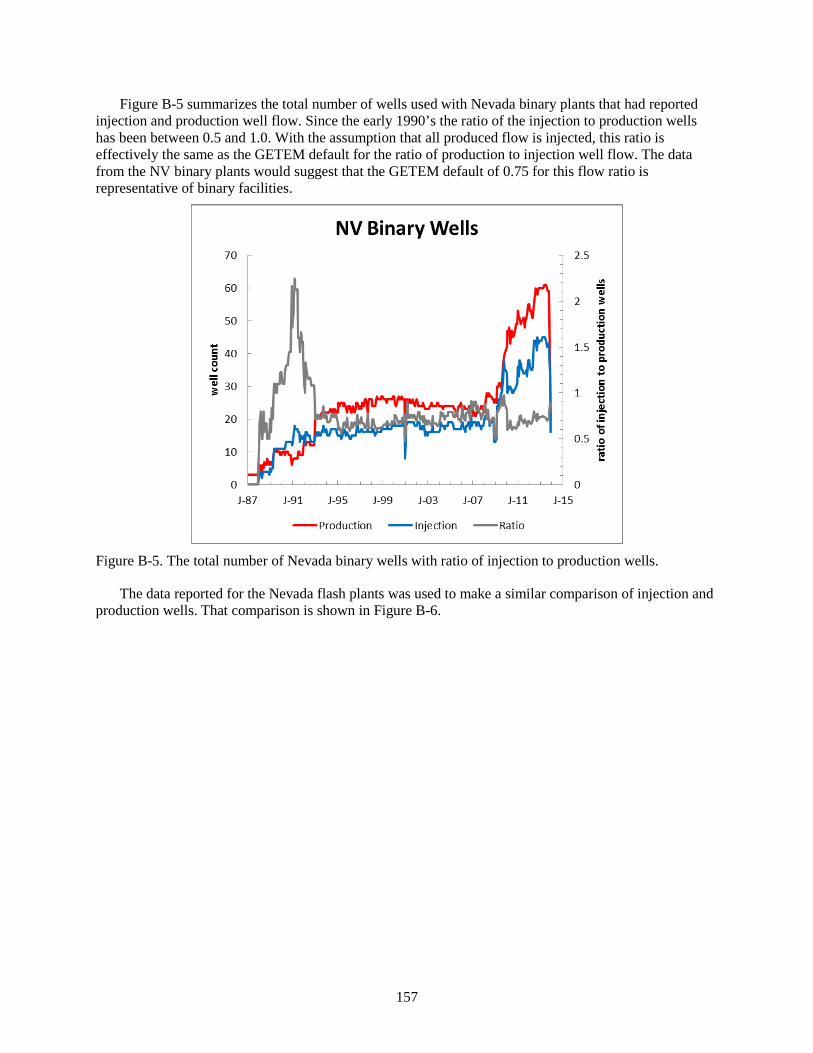
157

Figure B-5 summarizes the total number of wells used with Nevada binary plants that had reported injection and production well flow. Since the early 1990’s the ratio of the injection to production wells has been between 0.5 and 1.0. With the assumption that all produced flow is injected, this ratio is effectively the same as the GETEM default for the ratio of production to injection well flow. The data from the NV binary plants would suggest that the GETEM default of 0.75 for this flow ratio is representative of binary facilities.

Figure B-5. The total number of Nevada binary wells with ratio of injection to production wells.

The data reported for the Nevada flash plants was used to make a similar comparison of injection and production wells. That comparison is shown in Figure B-6.

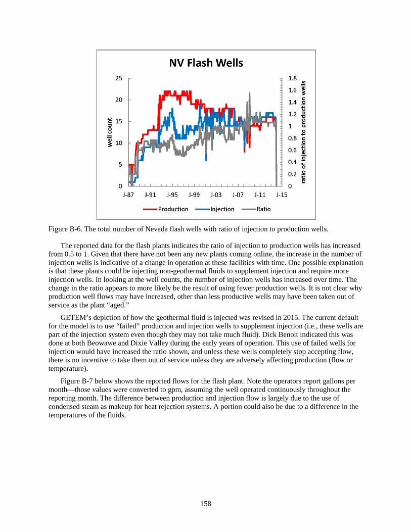
158

Figure B-6. The total number of Nevada flash wells with ratio of injection to production wells.

The reported data for the flash plants indicates the ratio of injection to production wells has increased from 0.5 to 1. Given that there have not been any new plants coming online, the increase in the number of injection wells is indicative of a change in operation at these facilities with time. One possible explanation is that these plants could be injecting non-geothermal fluids to supplement injection and require more injection wells. In looking at the well counts, the number of injection wells has increased over time. The change in the ratio appears to more likely be the result of using fewer production wells. It is not clear why production well flows may have increased, other than less productive wells may have been taken out of service as the plant “aged.”

GETEM’s depiction of how the geothermal fluid is injected was revised in 2015. The current default for the model is to use “failed” production and injection wells to supplement injection (i.e., these wells are part of the injection system even though they may not take much fluid). Dick Benoit indicated this was done at both Beowawe and Dixie Valley during the early years of operation. This use of failed wells for injection would have increased the ratio shown, and unless these wells completely stop accepting flow, there is no incentive to take them out of service unless they are adversely affecting production (flow or temperature).

Figure B-7 below shows the reported flows for the flash plant. Note the operators report gallons per month—those values were converted to gpm, assuming the well operated continuously throughout the reporting month. The difference between production and injection flow is largely due to the use of condensed steam as makeup for heat rejection systems. A portion could also be due to a difference in the temperatures of the fluids.

159

Figure B-7. Reported production and injection flows for Nevada flash wells.

The reported flows have decreased with time (as have the number of production wells). This would suggest:

1. the operator continues to use all available injection capacity, and/or

2. mineral precipitation has occurred in the well bore or formation that limits the ability of the injection wells to accept flow.

Supplemental Use of Failed Wells When drilling wells, presumably those considered “failures” lack fluid, temperature, and/or

permeability. Based upon discussions with industry, the use of “failed” wells to supplement injection appears to have been common, especially with the older plants in Nevada. Though this supplemental usage is likely to vary between projects, it is now the default for GETEM’s characterization of hydrothermal resources. In order to estimate the number of injection wells that are required, it is necessary that an assumption be made of the relative permeability of the “failed” wells that supplement injection. A relative flow was established for these supplemental wells using the data reported to the Division of Minerals by the geothermal operators in Nevada. The following assumptions were made:

• When flow is reported for a well, it is assumed that the well took flow continuously throughout the month at a constant rate.

• For a well to be considered used for supplemental injection, it had to have 12 months or more of reported flow, unless the well had been used continuously since it began operation (brought online during the last year of report data—2013).

• Wells having an average flow that was 90% or more of the average flow of all wells were considered “successful” injection wells. Though the 90% value is somewhat arbitrary, the basis for this criteria is that if wells are being used for supplemental injection, they will suppress the average injection well flow for the facility.

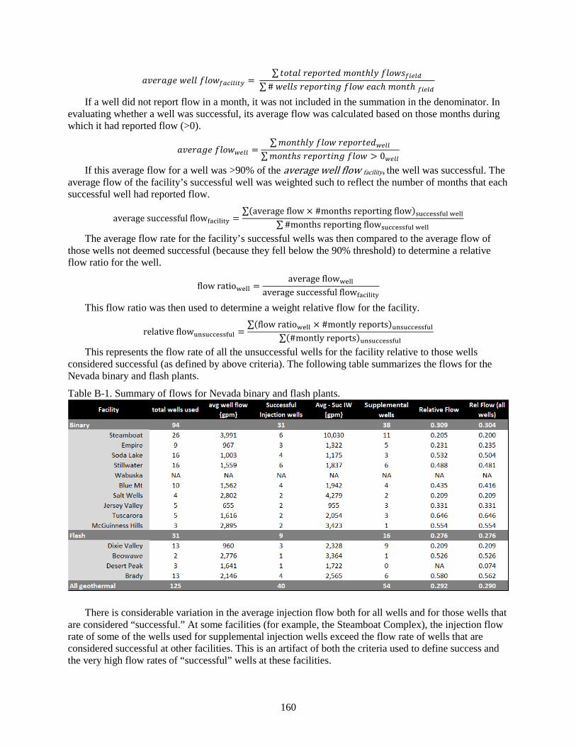
160

𝑆𝑆𝑙𝑙𝑃𝑃𝑃𝑃𝑆𝑆𝑃𝑃𝑃𝑃 𝑃𝑃𝑃𝑃𝑆𝑆𝑆𝑆 𝑓𝑓𝑆𝑆𝑃𝑃𝑃𝑃𝑓𝑓𝑝𝑝𝑎𝑎𝑓𝑓𝑓𝑓𝑓𝑓𝑛𝑛𝑎𝑎 = ∑𝑃𝑃𝑃𝑃𝑃𝑃𝑆𝑆𝑆𝑆 𝑃𝑃𝑃𝑃𝑃𝑃𝑃𝑃𝑃𝑃𝑃𝑃𝑃𝑃𝑑𝑑 𝑃𝑃𝑃𝑃𝑃𝑃𝑃𝑃ℎ𝑆𝑆𝑐𝑐 𝑓𝑓𝑆𝑆𝑃𝑃𝑃𝑃𝑆𝑆𝑓𝑓𝑓𝑓𝑛𝑛𝑓𝑓𝑓𝑓

∑# 𝑃𝑃𝑃𝑃𝑆𝑆𝑆𝑆𝑆𝑆 𝑃𝑃𝑃𝑃𝑃𝑃𝑃𝑃𝑃𝑃𝑃𝑃𝑃𝑃𝑃𝑃𝑃𝑃 𝑓𝑓𝑆𝑆𝑃𝑃𝑃𝑃 𝑃𝑃𝑆𝑆𝑃𝑃ℎ 𝑃𝑃𝑃𝑃𝑃𝑃𝑃𝑃ℎ 𝑓𝑓𝑓𝑓𝑛𝑛𝑓𝑓𝑓𝑓

If a well did not report flow in a month, it was not included in the summation in the denominator. In evaluating whether a well was successful, its average flow was calculated based on those months during which it had reported flow (>0).

𝑆𝑆𝑙𝑙𝑃𝑃𝑃𝑃𝑆𝑆𝑃𝑃𝑃𝑃 𝑓𝑓𝑆𝑆𝑃𝑃𝑃𝑃𝑤𝑤𝑛𝑛𝑓𝑓𝑓𝑓 =∑𝑃𝑃𝑃𝑃𝑃𝑃𝑃𝑃ℎ𝑆𝑆𝑐𝑐 𝑓𝑓𝑆𝑆𝑃𝑃𝑃𝑃 𝑃𝑃𝑃𝑃𝑃𝑃𝑃𝑃𝑃𝑃𝑃𝑃𝑃𝑃𝑑𝑑𝑤𝑤𝑛𝑛𝑓𝑓𝑓𝑓

∑𝑃𝑃𝑃𝑃𝑃𝑃𝑃𝑃ℎ𝑆𝑆 𝑃𝑃𝑃𝑃𝑃𝑃𝑃𝑃𝑃𝑃𝑃𝑃𝑃𝑃𝑃𝑃𝑃𝑃 𝑓𝑓𝑆𝑆𝑃𝑃𝑃𝑃 > 0𝑤𝑤𝑛𝑛𝑓𝑓𝑓𝑓

If this average flow for a well was >90% of the average well flow facility, the well was successful. The average flow of the facility’s successful well was weighted such to reflect the number of months that each successful well had reported flow.

average successful flowfacility =∑(average flow × #months reporting flow)successful well

∑#months reporting flowsuccessful well

The average flow rate for the facility’s successful wells was then compared to the average flow of those wells not deemed successful (because they fell below the 90% threshold) to determine a relative flow ratio for the well.

flow ratiowell =average flowwell

average successful flowfacility

This flow ratio was then used to determine a weight relative flow for the facility.

relative flowunsuccessful =∑(flow ratiowell × #montly reports)unsuccessful

∑(#montly reports)unsuccessful

This represents the flow rate of all the unsuccessful wells for the facility relative to those wells considered successful (as defined by above criteria). The following table summarizes the flows for the Nevada binary and flash plants.

Table B-1. Summary of flows for Nevada binary and flash plants.

There is considerable variation in the average injection flow both for all wells and for those wells that are considered “successful.” At some facilities (for example, the Steamboat Complex), the injection flow rate of some of the wells used for supplemental injection wells exceed the flow rate of wells that are considered successful at other facilities. This is an artifact of both the criteria used to define success and the very high flow rates of “successful” wells at these facilities.

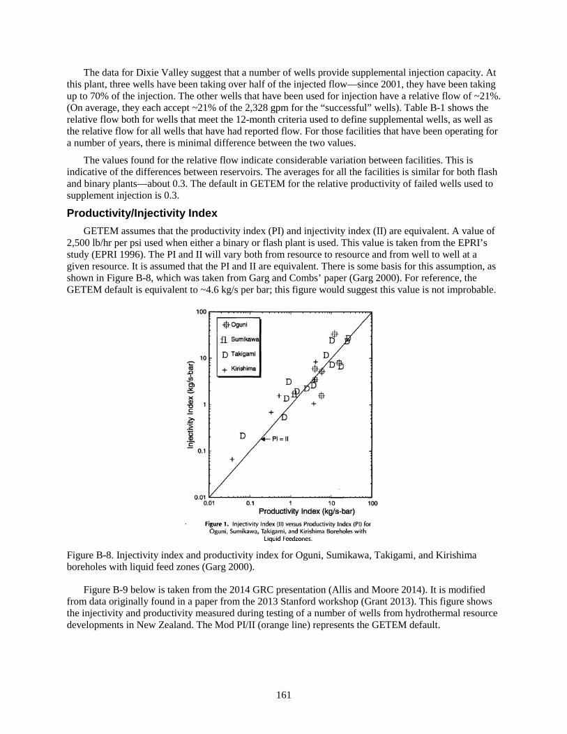
161

The data for Dixie Valley suggest that a number of wells provide supplemental injection capacity. At this plant, three wells have been taking over half of the injected flow—since 2001, they have been taking up to 70% of the injection. The other wells that have been used for injection have a relative flow of ~21%. (On average, they each accept ~21% of the 2,328 gpm for the “successful” wells). Table B-1 shows the relative flow both for wells that meet the 12-month criteria used to define supplemental wells, as well as the relative flow for all wells that have had reported flow. For those facilities that have been operating for a number of years, there is minimal difference between the two values.

The values found for the relative flow indicate considerable variation between facilities. This is indicative of the differences between reservoirs. The averages for all the facilities is similar for both flash and binary plants—about 0.3. The default in GETEM for the relative productivity of failed wells used to supplement injection is 0.3.

Productivity/Injectivity Index GETEM assumes that the productivity index (PI) and injectivity index (II) are equivalent. A value of

2,500 lb/hr per psi used when either a binary or flash plant is used. This value is taken from the EPRI’s study (EPRI 1996). The PI and II will vary both from resource to resource and from well to well at a given resource. It is assumed that the PI and II are equivalent. There is some basis for this assumption, as shown in Figure B-8, which was taken from Garg and Combs’ paper (Garg 2000). For reference, the GETEM default is equivalent to ~4.6 kg/s per bar; this figure would suggest this value is not improbable.

Figure B-8. Injectivity index and productivity index for Oguni, Sumikawa, Takigami, and Kirishima boreholes with liquid feed zones (Garg 2000).

Figure B-9 below is taken from the 2014 GRC presentation (Allis and Moore 2014). It is modified from data originally found in a paper from the 2013 Stanford workshop (Grant 2013). This figure shows the injectivity and productivity measured during testing of a number of wells from hydrothermal resource developments in New Zealand. The Mod PI/II (orange line) represents the GETEM default.

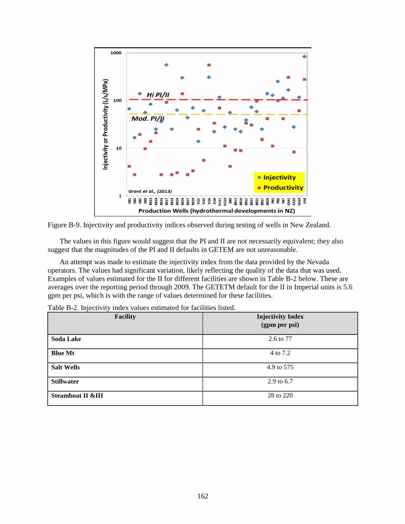
162

Figure B-9. Injectivity and productivity indices observed during testing of wells in New Zealand.

The values in this figure would suggest that the PI and II are not necessarily equivalent; they also suggest that the magnitudes of the PI and II defaults in GETEM are not unreasonable.

An attempt was made to estimate the injectivity index from the data provided by the Nevada operators. The values had significant variation, likely reflecting the quality of the data that was used. Examples of values estimated for the II for different facilities are shown in Table B-2 below. These are averages over the reporting period through 2009. The GETETM default for the II in Imperial units is 5.6 gpm per psi, which is with the range of values determined for these facilities.

Table B-2. Injectivity index values estimated for facilities listed. Facility Injectivity Index

(gpm per psi)

Soda Lake 2.6 to 77

Blue Mt 4 to 7.2

Salt Wells 4.9 to 575

Stillwater 2.9 to 6.7

Steamboat II &III 28 to 220

163

B2: RESERVOIR PRODUCTIVITY DECLINE: Nearly all geothermal resources experience some decline in productivity over time. This decline

could occur as reduced flow, temperature, and/or pressure of the produced geothermal fluid. Given that geothermal reservoirs have a finite size, a decline in productivity is not surprising. Conversion systems extract energy from the produced fluids and return it to the reservoir as a cooler fluid. The geothermal flow rates required to produce electrical power are relatively high. A 30 MW binary plant using a 175°C resource will produce just over 4 billion barrels of fluid over a 30-year life; this is over half the ~7 billion barrels of petroleum products consumed by the U.S. in 2015 (EIA). The 4 billion barrels used by the binary plant are equivalent to ~0.66 km3 of fluid, which would suggest that the produced fluid is cycled multiple times through the reservoir, mining the heat in place. The flash steam conversion system typically utilizes the steam condensate for makeup of the plant’s evaporative cooling system. As a consequence, less water is injected than is produced, potentially depleting the amount of fluid in the reservoir.

The liquid-dominated resources are more common and are the basis of GETEM’s depiction of a geothermal resource. This depiction assumes that the geothermal fluid entering the production zone in the well is a liquid, and remains a liquid at this point throughout the operating life of the well. GETEM characterizes the pressure decline that occurs using a productivity index (a model input) that is based upon the hydraulic pressure drawdown in the production well having reached a quasi-steady state value with time. With binary plants, the downhole production pumps offset the decline in reservoir pressure. Flash plants typically do not use production pumps, and the pressure drawdown impacts where flashing occurs in the production well.

The premise for GETEM’s estimates of how declining reservoir productivity impacts generation is based on the well flow rate remains constant with time and the pressure drawdown has reached its quasi steady state value. As such, neither flow nor pressure is included in GETEM’s characterization of declining resource productivity. This decrease in resource productivity is characterized as a declining resource temperature that is based on the following relationship:

𝑇𝑇𝑛𝑛 = 𝑇𝑇𝑓𝑓𝑛𝑛𝑓𝑓𝑛𝑛𝑓𝑓𝑝𝑝𝑓𝑓(1 − 𝑆𝑆𝑃𝑃𝑃𝑃𝑃𝑃𝑆𝑆𝑆𝑆 𝑑𝑑𝑃𝑃𝑃𝑃𝑆𝑆𝑃𝑃𝑃𝑃𝑃𝑃 𝑃𝑃𝑆𝑆𝑃𝑃𝑃𝑃)𝑛𝑛, where T is temperature, n is a point in time during the facility operation, and the annual decline rate % change in the temperature occurs annually (a GETEM input).

This relationship is used to determine the temperature of the produced fluid throughout the life of the project with GETEM’s assumption that all production wells are identical—that they have the same productivity index, and produce the same temperature and flow rate.

At a given point in time, the model uses this temperature and an ambient temperature to estimate the ideal work that could be accomplished by a power cycle. A second law efficiency is applied to this ideal work to calculate the actual work done, which is used as a net capacity factor to determine the plant’s net output at that point in time.

The declining resource temperature adversely impacts plant output and the power sales over the life of the project. This is illustrated in Figure B-10, which is GETEM’s estimate of the annual power generation for different rates of temperature decline.

164

Figure B-100. Effect of declining resource temperature on annual generation for sale.

As the resource productivity decreases, it is common for geothermal operators to increase the production flow to offset any significant impact on power generation. They will accomplish this by drilling additional wells and/or installing larger production pumps are greater depths. GETEM does not attempt to account for changes in production flow, as it is a site-specific activity and difficult to characterize for a “representative” plant. Instead, GETEM accounts for the impact of excessive temperature decline by replacing the entire well field once the decline reaches a maximum threshold value. In the model, this replacement occurs unless the project is in the last 5 years of its indicated life or insufficient resource potential was discovered to allow for replacement of the field (this resource potential is a model input). GETEM allows for multiple replacements as long as these two criteria are satisfied.

The default for the maximum temperature decline allowed is based on the end-of-project temperatures given in EPRI’s study (EPRI 1996). These values approximate a decline of ~10% in the Carnot efficiency as depicted here:

𝑇𝑇𝑝𝑝𝑛𝑛𝑝𝑝𝑓𝑓𝑝𝑝𝑎𝑎𝑛𝑛𝑝𝑝𝑛𝑛𝑛𝑛𝑛𝑛 =𝑇𝑇𝑔𝑔

�0.9 × � 𝑇𝑇𝑔𝑔𝑇𝑇𝑓𝑓𝑛𝑛𝑓𝑓𝑛𝑛𝑓𝑓𝑝𝑝𝑓𝑓

� + 0.1�

In this equation, all temperatures are absolute (either °K or °R), and To is the temperature to which heat is rejected (ambient). The current model default assumes that sufficient potential was discovered to allow for one well field replacement. In the scenario depicted in the above figure, GETEM would have replaced the well field once each for both the 0.8% and 1% decline rates.

With replacement, it is assumed that the produced fluid returns to the initial temperature, and that the power production returns to the original (design) output. The costs for the wells, pumps, and other components are included in the replacement costs and are discounted to determine their present value at startup (as are the revenues from the power sales) when determining the LCOE.

Though GETEM handles the effect of resource decline similarly for both flash steam and air-cooled binary plants, both have different default values for the temperature decline rate.

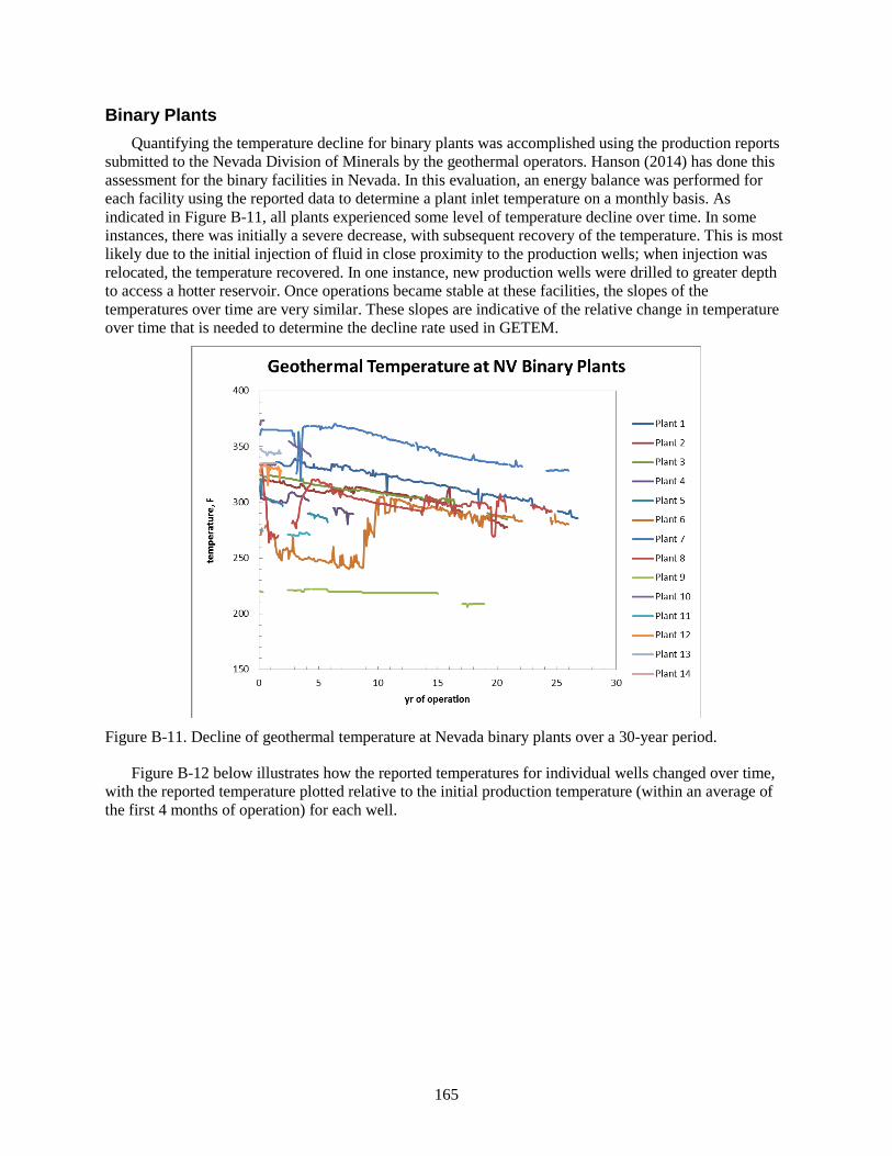
165

Binary Plants Quantifying the temperature decline for binary plants was accomplished using the production reports

submitted to the Nevada Division of Minerals by the geothermal operators. Hanson (2014) has done this assessment for the binary facilities in Nevada. In this evaluation, an energy balance was performed for each facility using the reported data to determine a plant inlet temperature on a monthly basis. As indicated in Figure B-11, all plants experienced some level of temperature decline over time. In some instances, there was initially a severe decrease, with subsequent recovery of the temperature. This is most likely due to the initial injection of fluid in close proximity to the production wells; when injection was relocated, the temperature recovered. In one instance, new production wells were drilled to greater depth to access a hotter reservoir. Once operations became stable at these facilities, the slopes of the temperatures over time are very similar. These slopes are indicative of the relative change in temperature over time that is needed to determine the decline rate used in GETEM.

Figure B-11. Decline of geothermal temperature at Nevada binary plants over a 30-year period.

Figure B-12 below illustrates how the reported temperatures for individual wells changed over time, with the reported temperature plotted relative to the initial production temperature (within an average of the first 4 months of operation) for each well.

166

Figure B-12. Reported wellhead temperature decline over time at Nevada binary facilities.

Except for a few wells that have only been in operation for a short time, these wells experienced a decline in temperature. Some experienced a rapid decline; if this decline was not mitigated by moving injection, these wells were typically taken out of service and not used. For some months, the reported temperatures were abnormally high or low. The higher values are likely errors in the reporting. The low values are either errors or reflect intermittent production from the well. Shown in Figure B-13 is a linear fit of all the data with the intercept at time 0 forced to be equal to 1. The slope of this line reflects the annual decline of the temperature for all wells relative to their initial operation. The decline of individual wells shown in this figure is of interest because if the rates differed significantly from that determined for the fluid entering the plants, it would suggest that there is significant post-startup replacement of wells.

In Figure B-13, the production temperatures determined for the Steamboat Complex facilities are shown as a function of time and total production flow. The solid black line in the figure on the left is a linear curve fit of data for all of the facilities. The slope of this line approximates the decline rate needed in GETEM. The figure on the right shows the temperature that is determined from the total enthalpy and total flow of the fluid entering all the producing binary facilities. This “weighted” temperature is plotted as a function of the cumulative flow of all facilities, beginning with the SBI plant. The colored symbols depict when the other facilities began operation. Steamboat Hills is a flash plant, and though its reported temperatures were not used in determining the temperatures shown, its reported flow was included in the running total flow produced. The value in parentheses after each plant’s name shown is the year it began reporting flow to the NV DoM.

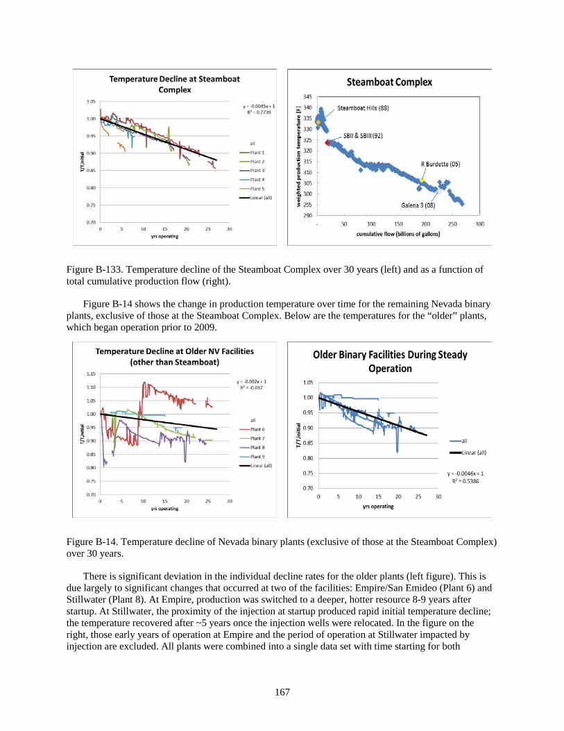
167

Figure B-133. Temperature decline of the Steamboat Complex over 30 years (left) and as a function of total cumulative production flow (right).

Figure B-14 shows the change in production temperature over time for the remaining Nevada binary plants, exclusive of those at the Steamboat Complex. Below are the temperatures for the “older” plants, which began operation prior to 2009.

Figure B-14. Temperature decline of Nevada binary plants (exclusive of those at the Steamboat Complex) over 30 years.

There is significant deviation in the individual decline rates for the older plants (left figure). This is due largely to significant changes that occurred at two of the facilities: Empire/San Emideo (Plant 6) and Stillwater (Plant 8). At Empire, production was switched to a deeper, hotter resource 8-9 years after startup. At Stillwater, the proximity of the injection at startup produced rapid initial temperature decline; the temperature recovered after ~5 years once the injection wells were relocated. In the figure on the right, those early years of operation at Empire and the period of operation at Stillwater impacted by injection are excluded. All plants were combined into a single data set with time starting for both

168

Stillwater and Empire once their operation had stabilized. With this adjustment to this data, the overall decline for these older facilities is similar to that determined for the Steamboat Complex.

Figure B-15 below shows the changes in production temperature for the newer binary facilities in Nevada. The gap in the temperatures represents a 2-year period during which they were not available in information provided by the NV DoM.

Figure B-15 Temperature decline for newer binary facilities in Nevada.

The decline rate found for the newer facilities was significantly higher than that for the older facilities. This is largely because of the temperature decline at Blue Mt. (Plant 10). With this facility removed from the data set, the slope of the linear fit is −0.004, which is similar to the older binary plants.

A fit of all the Nevada binary plant data, yields a slope of ~−0.003. This value is low primarily because of the impact of the Empire data. If the Empire data is excluded, the slope increases to −0.0042.

This assessment indicates that the slope of the relative decline is between −0.004 and −0.0046. Using these slopes, the annual temperature decline rate can be determined; that rate would vary from 0.42% to 0.48%. The relative change in the temperatures entering the plant are slightly lower than the overall relative change in the temperatures from all production wells. This would suggest that some re-drilling has occurred, with new wells being used to supplement initial production. If one were to use the slope of the decline for the production wells, the annual decline rate would be 0.56%. This rate does include wells that were taken out of service because they experienced a rapid initial decline in temperature. It is believed that the decline rates based on the temperature of the fluid entering the plants is more representative of the reservoirs.

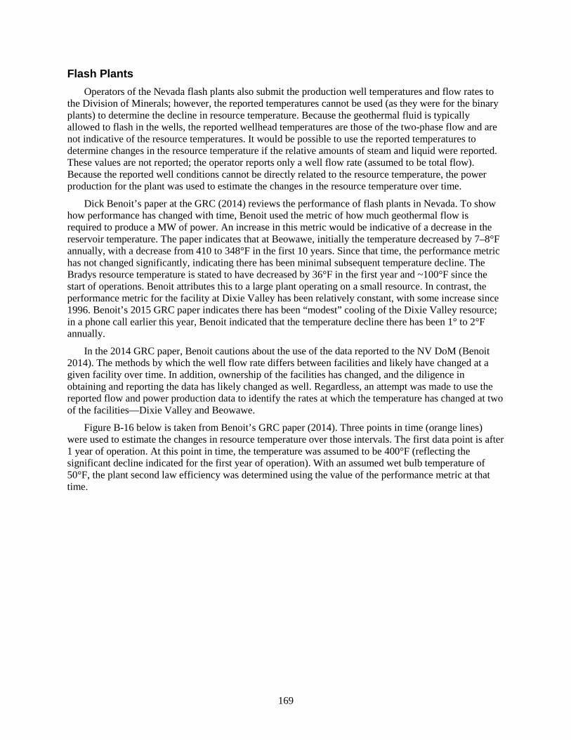
169

Flash Plants Operators of the Nevada flash plants also submit the production well temperatures and flow rates to

the Division of Minerals; however, the reported temperatures cannot be used (as they were for the binary plants) to determine the decline in resource temperature. Because the geothermal fluid is typically allowed to flash in the wells, the reported wellhead temperatures are those of the two-phase flow and are not indicative of the resource temperatures. It would be possible to use the reported temperatures to determine changes in the resource temperature if the relative amounts of steam and liquid were reported. These values are not reported; the operator reports only a well flow rate (assumed to be total flow). Because the reported well conditions cannot be directly related to the resource temperature, the power production for the plant was used to estimate the changes in the resource temperature over time.

Dick Benoit’s paper at the GRC (2014) reviews the performance of flash plants in Nevada. To show how performance has changed with time, Benoit used the metric of how much geothermal flow is required to produce a MW of power. An increase in this metric would be indicative of a decrease in the reservoir temperature. The paper indicates that at Beowawe, initially the temperature decreased by 7–8°F annually, with a decrease from 410 to 348°F in the first 10 years. Since that time, the performance metric has not changed significantly, indicating there has been minimal subsequent temperature decline. The Bradys resource temperature is stated to have decreased by 36°F in the first year and ~100°F since the start of operations. Benoit attributes this to a large plant operating on a small resource. In contrast, the performance metric for the facility at Dixie Valley has been relatively constant, with some increase since 1996. Benoit’s 2015 GRC paper indicates there has been “modest” cooling of the Dixie Valley resource; in a phone call earlier this year, Benoit indicated that the temperature decline there has been 1° to 2°F annually.

In the 2014 GRC paper, Benoit cautions about the use of the data reported to the NV DoM (Benoit 2014). The methods by which the well flow rate differs between facilities and likely have changed at a given facility over time. In addition, ownership of the facilities has changed, and the diligence in obtaining and reporting the data has likely changed as well. Regardless, an attempt was made to use the reported flow and power production data to identify the rates at which the temperature has changed at two of the facilities—Dixie Valley and Beowawe.

Figure B-16 below is taken from Benoit’s GRC paper (2014). Three points in time (orange lines) were used to estimate the changes in resource temperature over those intervals. The first data point is after 1 year of operation. At this point in time, the temperature was assumed to be 400°F (reflecting the significant decline indicated for the first year of operation). With an assumed wet bulb temperature of 50°F, the plant second law efficiency was determined using the value of the performance metric at that time.

170

Figure B-146. Monthly fluid production and conversion factor between 1986 and 2013 at Beowawe.

Assuming this efficiency remains constant, and using the 50°F wet bulb temperature, a resource temperature can be determined that produces the indicated performance metric in 1994 and again in 2005. With this approach, the resource temperature is estimated to be 320°F in 1994 and 306°F in 2005. Though the magnitude of these values change if different second law efficiency or wet bulb temperature are used, the magnitude of the estimated decline between 1994 and 2005 would not change that much. This approach indicates that over this 11-year period, the temperature decreased by ~14°F.

A similar approach was used for Dixie Valley based on Figure B-17 below (from Benoit’s 2014 paper). The time period of interest was from 1996 to 2012 when a binary bottoming unit began operating at the facility. To produce the change in the performance metric, the temperature decreased by ~30°F over this 16-year period. This value is consistent with anecdotal value that Benoit provided.

171

Figure B-17. Monthly fluid production and conversion factor between 1988 and 2013 at Dixie Valley.

There are issues with this approach, one of which is that the plant conversion efficiency does not remain constant. Invariably, when either the brine flow or temperature deviates from the design value, the second law efficiency changes (likely decreases). A decreased efficiency would increase the temperatures needed to produce indicated levels of performance.

To account for the impact of the efficiency, the design information for each plant was taken from Benoit’s 2014 GRC paper (geothermal temperature and flow rate, as well as net power). Using the assumed wet bulb temperature of 50°F, a model of a “pseudo” dual-flash plant was developed and used to estimate the impact of varying geothermal temperatures and flow rates on the plant output. These results were used to develop a correlation for each plant that estimated the impact of changes to both flow and temperature on the second law conversion efficiency. The correlations were then applied to the monthly data reported to the NV DoM for each plant. To account for changing ambient conditions, an average monthly wet bulb temperature for Winnemucca, Nevada was applied (NOAA). This ambient data set was used for both the Beowawe and Dixie Valley facilities. With the geothermal flow rate and the wet bulb temperature, the resource temperature needed to produce the reported power output to the NV DoM could be determined.

Figure B-18 has the temperatures determined for Dixie Valley. The initial resource temperature was ~480°F (Benoit, 2015).

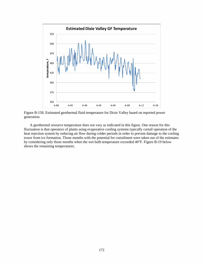
172

Figure B-158. Estimated geothermal fluid temperature for Dixie Valley based on reported power generation.

A geothermal resource temperature does not vary as indicated in this figure. One reason for this fluctuation is that operators of plants using evaporative cooling systems typically curtail operation of the heat rejection system by reducing air flow during colder periods in order to prevent damage to the cooling tower from ice formation. Those months with the potential for curtailment were taken out of the estimates by considering only those months when the wet bulb temperature exceeded 40°F. Figure B-19 below shows the remaining temperatures.

173

Figure B-19. Estimated geothermal fluid temperature for Dixie Valley based on reported power generation when wet bulb temperature exceeded 40°F.

The absolute magnitude of the estimated temperatures is not of importance other than they should approach the value expected at the beginning of operation. What is of interest is the change that occurs in the estimates over time. The estimates shown indicate that the temperature has declined beginning in about 1996. Benoit’s GRC papers (2014 & 2015) indicate that from startup through 1997, production and injection capacity were changing, with new wells being brought into service; this likely contributes to the apparent increase in temperature occurring after operation began in 1988. The estimates suggest there was an apparent slight temperature recovery in 2004, after which it again declined. This recovery is likely the effect of a modification to the turbine to lower operating pressures and improve its efficiency (Benoit 2015).

Using this data, and considering the period from 1996 through 2010, the temperature decreased ~40°F which is more than the decrease that was estimated using the plots in Benoit’s paper (2015). Data was not considered for 2011 because, during that year, the reported flow rate was ~10–13% higher than the design value that was used. While the approach used to estimate the temperatures included the effect of varying flow, excluding that year was believed to improve the estimate of the decline rate. Excluding all calculated temperatures above 500°F, an annual decline rate of 0.58% was determined for this period (including the higher temperature estimates, increased the decline rate to ~0.64%).

The similar approach was used to estimate the change in the geothermal fluid temperature over time at Beowawe. The estimated temperatures are shown in Figure B-20 below. The temperature of this resource was ~410°−420°F at startup.

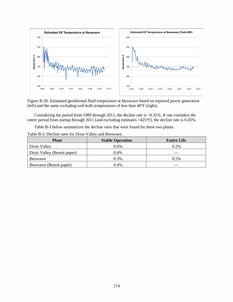
174

Figure B-20. Estimated geothermal fluid temperature at Beowawe based on reported power generation (left) and the same excluding web bulb temperatures of less than 40°F (right).

Considering the period from 1989 through 2011, the decline rate is ~0.31%. If one considers the entire period from startup through 2011 (and excluding estimates >425°F), the decline rate is 0.45%.

Table B-3 below summarizes the decline rates that were found for these two plants.

Table B-3. Decline rates for Dixie Valley and Beowawe. Plant Stable Operation Entire Life

Dixie Valley 0.6% 0.2% Dixie Valley (Benoit paper) 0.4% — Beowawe 0.3% 0.5% Beowawe (Benoit paper) 0.4% —

175

176

REFERENCES Allis, R. and J. Moore, 2014, “Can Deep Stratigraphic Reservoirs Sustain 100 MW Power Plants?”

Geothermal Resources Council Transactions, Vol. 38, pp. 1009–1016.

Benoit, D., 2014, “The Long Term Performance of Nevada Geothermal Fields Utilizing Flash Plant Technology,” Geothermal Resources Council Transactions, Vol 38, pp. 997–984.

Benoit, D., 2015, “A Case History of the Dixie Valley Geothermal Field,” Geothermal Resources Council Transactions, Vol. 39.

California Independent System Operator, Pacific Gas and Electric Company, https://www.caiso.com/informed/Pages/StakeholderProcesses/ParticipatingTransmissionOwnerPerUnitCosts.aspx.

Clemo, T., 2006, “Flow in Perforated Pipes: A Comparison of Models and Experiments,” Society of Petroleum Engineers Production and Operations, May 2006, pp. 302–311.

Crane, 1942, Technical Paper 410, TP-410.

DiPippo, R., 2012, Geothermal Power Plants: Principles, Applications, Case Studies and Environmental Impact, Waltham, Massachusetts: Elsevier.

EERE, 2013, “Cooling Towers: Understanding Key Components of Cooling Towers and How to Improve Water Efficiency,” http://energy.gov/sites/prod/files/2013/10/f3/waterfs_coolingtowers.pdf.

EIA, 2015, U.S. Energy Information Administration Frequently Asked Questions, “How much oil is consumed in the United States?” http://www.eia.gov/tools/faqs/faq.cfm?id=33&t=6.

EPRI, 1996, Next Generation Geothermal Power Plants, TR-106223, April 5, 1996.

ESMAP, 2012, Geothermal Handbook: Planning and Financing Power Generation, 72828, September 24, 2012.

Fournier, R. 1981, “Application of water geochemistry to geothermal exploration and reservoir engineering,” Geothermal Systems: Principles and Case Histories, Edited by Rybach and L. Muffler, Eds, Wiley, New York.

Gallup, D and E. Barcelon, 2005, “Investigations of Organic Inhibitors for Silica Scale Control from Geothermal Brines – II,” Geothermics, Vol. 34, pp. 756–771.

Garg, S.K. and J. Combs, 2000, “Geothermal Reservoir Assessment Using Data from Slim Holes,” Geothermal Resources Council Transactions, Vol. 24, pp. 581–587.

Grant, M., J. Clearwater, J. Quinao, P. Bixley, and M. LeBrun, 2013, “Thermal Stimulation of Geothermal Wells: A Review of Field Data,” Proceedings of Thirty-Eight Workshop on Geothermal Reservoir Engineering, Stanford University, Stanford, California, February 11–13, 2013..

Green, D.W. and R.H. Perry, Perry’s Chemical Engineers’ Handbook, New York: McGraw-Hill.

Gunnarsson, I. and Arnorsson, S., 2000, “Amorphous silica solubility and the thermodynamic properties of H4SiO°4 in the range of 0° to 350°C at Psat,” Geochimica et Cosmochimica Acta, Vol. 64, No. 13, pp. 2295–2307.

Hagerty, S., 2014, “Geothermal Energy Leasing on BLM Managed Lands,” Geothermal Research Council Pre-Meeting Workshop, Portland, Oregon, September 26, 2014.

177

Hanson, H. and G. Mines, 2014, “Summary of Historical Production for Nevada Binary Facilities,” Proceedings of the Thirty-Eighth Geothermal Resources Council Annual Meeting and GEA Geothermal Energy Expo, Portland, Oregon, September 28–October 1, INL/CON-14-31966.

Internal Revenue Service, 2015, How to Depreciate Property, Publication 946.

NOAA, Climate Data Online, https://www.ncdc.noaa.gov/cdo-web/.

PG&E, 2009, Pacific Gas and Electric Company Stakeholder Meeting, Folsom, California, February 26, 2009, http://www.caiso.com/2360/23609c2864470.pdf.

Price, W.G. and L. Burleigh, 2001, “Electric Submersible Pumps for Geothermal Resources,” GRC Transactions, Vol. 25, pp. 27–31.

Public Law 103-62, 1993, “Government Performance Results Act of 1993,” United States Congress, August 3, 1993.

Ramey, H.J. Jr., 1962, “Wellbore Heat Transmission,” Journal of Petroleum Technology, Vol. 14. No. 4, pp. 427–435.

Sanyal, S.K. and J.W. Morrow, 2012, “Success and the Learning Curve Effect in Geothermal Well Drilling—A Worldwide Survey,” Proceedings of the Thirty-Seventh Workshop on Geothermal Reservoir Engineering, Stanford University, Stanford, California, January 30–February 1, 2012, SGP-TR-194.

Tetra Tech, 2008, California’s Costal Power Plants: Alternative Cooling System Analysis, prepared for California Ocean Protection Council, February 2008

Tidwell, V.C., K. Zemlick, and G. Klise, 2013, “Nationwide Water Availability Data for Energy-Water Modeling,” SAND2013-9968, November 2013.

United States Department of Labor, Bureau of Labor Statistics, Producer Price Indexes, http://www.bls.gov/ppi/, February 2016.

Xie, X., K. Bloomfield, G. Mines, and M. Shook, 2005, “Design Considerations for Artificial Lifting of EGS Fluids,” Proceedings of the Geothermal Resources Council, Reno, Nevada, September 25–28, Vol. 29, pp. 801–806.