getting back to full employment - a better bargain for working people - by dean baker
DESCRIPTION
Getting Back to Full Employment - A Better Bargain for Working People - By Dean BakerTRANSCRIPT


Getting Back to Full Employment
A Better Bargain for Working People
By Dean Baker
and
Jared Bernstein
Published by the Center for Economic and Policy Research
Washington, DC

Published by the Center for Economic and Policy Research
1611 Connecticut Ave. NW, Suite 400
Washington, DC 20009
www.cepr.net
Cover design by Justin Lancaster
Creative Commons (cc) 2013 by Dean Baker and Jared Bernstein
Notice of rights: This book has been published under a Creative
Commons license. This work may be copied, redistributed, or displayed
by anyone, provided that proper attribution is given.
ISBN: 978-0-615-91835-8


Getting Back to Full Employment: A Better Bargain for Working People i
Contents
Contents ........................................................................................................ i
Acknowledgements ..................................................................................... iii
1 Introduction ............................................................................................. 1
2 Evidence of the Benefits of Full Employment .......................................... 7
Data Appendix ...................................................................................... 19
3 Structural Unemployment ..................................................................... 21
4 Full Employment and the Budget .......................................................... 46
5 Policies for Full Employment I ................................................................ 56
6 Policies for Full Employment II ............................................................... 72
7 Full Employment Now ............................................................................ 94
References ................................................................................................ 97


Getting Back to Full Employment: A Better Bargain for Working People iii
Acknowledgements
This book might not exist were it not for the help we got from many
others.
John Schmitt’s input—including number crunching and advice—was
indispensable. His fingerprints are all over the book, but especially on Chapter 2.
Pat Watson, editor extraordinaire, has been turning “economese” into
English for decades and we know of no one who does it better. His value added is
obvious on every page.
The data resources of the Economic Policy Institute, where we met years
ago, were also essential. EPI has become a “Bureau of Labor Statistics” for tracking
the economy faced by working families. The rigor and depth of their data
resources have made a huge contribution to the most critical economic debates of
our time, including inequality and full employment.
We also thank Arloc Sherman and William Chen from the Center On
Budget and Policy Priorities for helping with data collection. Bernstein thanks the
CBPP for their support, encouragement, and the tolerance of a lot of badgering of
busy people about stuff they’re not doing at the moment. Dean Baker thanks his
colleagues at the Center for Economic and Policy Research for their support and
assistance, especially Alan Barber, Nicole Woo, Milla Sanes, and Matthew Sedlar
who did so much to keep this book moving forward as we missed deadline after
deadline.
Finally Dean would like to thank Biscuit, Riley, Olive and especially
Helene for their endless patience and unconditional love. Jared Bernstein thanks
his family – Kay, Kate, Ellie, Sarah, Gary, Stripey, and Blackness--for all their
unending support.


Getting Back to Full Employment: A Better Bargain for Working People 1
Chapter 1
Introduction
What a difference a decade makes.
In the year 2000, when today’s 30-year olds were about 17, wrapping
up high school and on the cusp of looking for work or heading to college, the
unemployment rate in the United States averaged 4.0 percent. The last time it
was that low was during the “Age of Aquarius,” in 1969. Since 2000, it has
never been that low again. When we wrote an earlier version of this book in
2003, the sun had set on the age of full unemployment. As we revisit this
critical issue, the jobless rate has ranged from 7 percent to 10 percent for over
four years, and it’s not expected to come down much anytime soon.
A strong labor market with full employment need not be a rare
economic anomaly that returns roughly twice for every one appearance of
Halley’s Comet. Full employment can be a regular feature of the policy
landscape, with tremendous benefits for rising living standards, poverty
reduction, the federal budget, and equitable economic growth. In this book we
present the benefits and importance of full employment in ways that are
particularly germane to the economy today, and we offer policies to begin
moving to full employment now.
Full employment can be defined as the level of employment at which
additional demand in the economy will not create more employment. All
workers who seek a job have one, they are working for as many hours as they
want to or can, and they are receiving a wage that is broadly consistent with
their productivity. The only people in the labor market not working are the

2 Dean Baker and Jared Bernstein
ones who do not have the skill or ability to work (the structurally
unemployed) and those who are between jobs (the frictionally unemployed). It
is reasonable to argue that we were approaching this level in 2000.
When demand in the economy can no longer create more
employment, where does the pressure find an outlet? The obvious answer is
higher prices, as purchasers bid up the price of goods and employers bid up the
price of workers. To acknowledge this relationship between low
unemployment and price pressure is common sense. But there is a huge
difference between acknowledging the relationship and believing that public
policy must avoid full employment because it will cause inflation, or that it
must tolerate a cruelly high level of unemployment simply to avoid a slight risk
of inflation.
In the conventional view, the unemployment rate associated with full
employment and stable inflation is called the non-accelerating inflation rate of
unemployment, or NAIRU. Hiring when the unemployment rate is below the
NAIRU, the story goes, will lead to unsustainable price pressures: Workers
will come to be in such short supply that the growth rate in their wages will
rise above the growth rate of their productivity, forcing employers to raise
prices in order to maintain profit margins. When workers see that prices have
risen, they will seek even higher wages, pushing costs higher still for
employers. This wage–price spiral eventually spins out of control. As we said,
this is the conventional view, but the actual story in the real world is not likely
to be this simple, and we have less to fear from a wage–price spiral than many
economists insist we do. (We discuss this issue in Chapter 3.)
The relatively straight line in Figure 2-1 in Chapter 2 shows the
Congressional Budget Office (CBO) estimates of the NAIRU; the more erratic
line is the actual unemployment rate.1 The comparison enables a few pertinent
1 While we believe it is not possible to be this precise about the level of the NAIRU at a point in time, there are good reasons to use CBO’s series. First, it represents the industry standard for the unemployment rate associated with full employment; second, the values CBO derives are generally going to be close to the actual full employment rate (with the exception of the mid-1990s, when CBO’s estimate turned out to be well above the rate consistent with full employment); and third, though we can argue about the precise number, the nation would be well-served today were we to shoot for CBO’s current NAIRU of 5.5 percent.
Getting Back to Full Employment: A Better Bargain for Working People 3
observations about full employment, regardless of your thoughts about the
NAIRU:
Since the 1980s, the job market has spent a lot more time above than
below the NAIRU, i.e., it has had a lot of slack. Not coincidentally,
over those years wages have stagnated and income inequality has
grown.
The NAIRU is not constant. It slowly drifts up and down based on the
changing relationships between unemployment and inflation, as well
as changes in the characteristics of the workforce. This makes it tricky,
and less useful from a policy perspective, to pin the NAIRU down to a
precise percentage-point estimate.
During much of the 1990s the unemployment rate was below the
CBO’s NAIRU. In those years, not only did compensation rise across
the workforce, but low-wage workers made particularly strong gains,
poverty rates fell sharply, and, for the first time in years, middle-class
incomes rose in tandem with productivity growth. Yet, inflation
actually grew more slowly.
Since the Great Recession, the job market has been exceedingly slack,
and virtually all the progress noted above has unwound.
Why another look at full employment?
Since our last book in 2003, a number of developments have led us
back to this research.
First, many analysts and policymakers wrongly believe that one reason
unemployment remains elevated is because of a pervasive mismatch between
the skills that employers demand and those that workers are bringing to the
table. These analysts, who range from former President Clinton to industry
titans like General Electric’s Jeff Immelt, believe that too many in the
workforce lack the skills they need to get a job in today’s labor market, no

4 Dean Baker and Jared Bernstein
matter how hard they look. 2 Their unemployment, in other words, is
structural. It would persist even if the economy were humming along.
As we emphasize in Chapter 3, we’re sure this is not the case. In fact,
pundits were making the same argument in the early 1990s, only to find that as
the economy approached full employment, these workers found jobs and
contributed handily to the economy’s growth. There is copious evidence that
we’re in a cyclical, not a structural, slump. That’s not to say everyone is
adequately skilled or that lower-skilled workers couldn’t benefit from more
training. But the U.S. economy is capable of producing many millions more
jobs for workers at all skill levels and, were it to do so, workers who appear to
the punditry to be unfit for work would be miraculously on the job.
A second new development that brings us back to this research is
inflation targeting by the Federal Reserve Board. Fed Chairman Ben Bernanke
has publicly committed the central bank to a policy of targeting a 2.0 percent
inflation rate. While there are different ways in which this target can be
interpreted, one way that other central banks have interpreted it is to focus on
the target as their only policy goal. But the Fed has a mandate from Congress
to pursue full employment, and departing from this mandate could mean
keeping the unemployment rate unnecessarily high for long periods.
Finally, unemployment remains historically and stubbornly high, and
policymakers need to take action now to bring down the unemployment rate.
We put forth here a number of ideas that would put people back to work and
boost our anemic growth rates, even though it’s clear that the failure of the
political system to respond to our current jobs crisis is not due to a lack of
good ideas. Instead, policymakers’ intransigence has been a function of
partisan politics and two fundamental errors in judgment:
Misplaced concerns about the budget deficit – the failure to recognize
that temporarily larger budget deficits are necessary for growth and
jobs right now, and will not drive future deficits. To the contrary, as
we emphasize in Chapter 4, full employment should be considered an
ally of those who seek a more balanced budget.
2 See Immelt and Chenault (2011).

Getting Back to Full Employment: A Better Bargain for Working People 5
Misunderstanding the impact of the American Recovery and
Reinvestment Act (ARRA) – the 2009 stimulus was an effective job
creator, though not all of its programs were as effective as others.
Research has given us a good idea as to which measures had the biggest
bang-for-the-buck on job creation, and instead of caterwauling about
the “failed stimulus” we should take advantage of this information to
bring down the unemployment rate.3
Yet, it will likely take more than short-term stimulus measures to
maintain full employment in the future. While there is no evidence that the
structural problem of a pervasive skills mismatch is holding us back on the
supply side of the labor market, we are facing structural deficiencies on the
demand side. That is, the market is not providing enough gainful employment
opportunities for all comers into the workforce.
It just so happens that at the same time we have a crisis of deficient
structural demand, we also have a crisis of crumbling infrastructure. America’s
once-world-class systems of transportation (roads, bridges, rail beds, airports),
the power grid, the water supply, public buildings and spaces (schools, parks,
offices, and sidewalks), and research and development are deteriorating, and it
is hurting our productivity and our living standards.
Addressing the poor state of our infrastructure in a period of high
unemployment would be a perfect marriage of demand and supply. But we can
also be more forward looking. Our per capita energy use is about twice as high
as energy use in European countries that have comparable living standards.
Much of our excess use is simply due to waste, and we can create well-paying
jobs by resolving to make our homes, cars, offices, and other buildings more
efficient (Pollin 2012).
We can also look at changing the structure of work as a way to
generate jobs. A full-time job in the United States typically means working
many more hours a year than it does in Germany, the United Kingdom, or
other wealthy countries. In those countries, four to six weeks a year of paid
3 Michael Grunwald’s book, The New New Deal, provides an extensive analysis of the effectiveness of the Recovery Act.

6 Dean Baker and Jared Bernstein
vacation is the norm, and nearly everyone can count on paid sick days and paid
parental leaves. As a simple arithmetic proposition, if everyone worked 20
percent fewer hours and cut back their work accordingly, then employers
would have to create roughly 20 percent more jobs. The real world is more
complicated, but the basic logic holds, other things being equal: If the typical
worker puts in less time on the job, more people will have jobs.
We should also recognize that some people will find it almost
impossible to find jobs given the current state of the economy. In particular, in
many areas the teen unemployment rate exceeds 50 percent. In effect, there
are no jobs for teens. It is not fair to ask them to wait until the policymakers
can figure out how to fix the economy. We should be looking to give young
people jobs now, even if that means the direct creation of jobs by the
government. Conservatives can disparage these as “make-work jobs,” but there
is solid, conventional economics behind this: If the market fails to provide
those willing to work a chance to contribute to national output, then policy
must intervene to fix that market failure, and in this case there is the added
benefit of giving people an opportunity in life. It’s not the fault of the typical
unemployed teenager that virtually all of the economic authorities failed to
recognize an $8 trillion housing bubble.
We believe there are few if any economic policy issues as important as
full employment. It is essential for reducing the income stagnation that has
beset the middle class, reducing poverty rates among working-age families,
pushing back against economic inequality, and improving our fiscal outlook.
Today’s dysfunctional politics are doing nothing helpful to get us there. To the
contrary, policymakers in advanced economies are embracing “austerity”
measure that push the other way.
That is why it is important to lay out the case for full employment and
the path for getting there. The logic and evidence for full employment are
strong, and someday, hopefully soon, logic and evidence will matter again.

Getting Back to Full Employment: A Better Bargain for Working People 7
Chapter 2
Evidence of the Benefits of Full Employment
The historical record in the United States supports the notion that,
when labor markets are tight, the benefits of growth are more likely to flow to
the majority of working people. Conversely, when there’s slack in the job
market, as has been the case more often than not in recent years, working
families fall behind.
Job markets operating below full employment are not confined to
recessions. Business cycle expansions over the past 30 years have featured
labor markets with too much slack to provide workers with the bargaining
clout they need to claim their share of the growth they’re helping to produce
(the later 1990s were an important exception). Moreover, the last three
recessions have been followed by initially weak “jobless” and “wageless”
recoveries, implying that, in recent years, incomes and wages have failed to
get much of a lift in bad times or good ones.
Indeed, the post-1970s period of slack job markets has also been a
period of low- and middle-wage stagnation and rising wage and income (and
wealth) inequality. The absence of full employment in most years since the
1970s was not the only factor in play; the reasons for the rise in inequality
include globalization, technological change, a bubble-driven finance sector
claiming disproportionate profit shares, declining unions, a falling value of the
minimum wage, and more.

8 Dean Baker and Jared Bernstein
But slack employment and its corollary – diminished bargaining power
– get overlooked, in no small part because policymakers assume full
employment is out of their control, though it is decidedly not. To give up on
full employment is a mistake, because in an economy in which collective
bargaining is minimal in the private sector and under siege in the public sector,
full employment is the only route for working Americans can get ahead. Rising
living standards for the majority require a labor market that is tight enough to
force employers to raise compensation to the level where they can attract and
keep the workers they need. Whenever that force has been in place, working
people have done much better than when it’s been absent.
Growing together or growing apart,
and the role of full employment
As discussed in Chapter 1, economists don’t have a good track record
in terms of quantifying a reliable definition of full employment or the costs of
setting the NAIRU – the unemployment rate generally associated with non-
inflationary full employment – so high that it sacrifices growth and jobs,
particularly for less-advantaged persons whose incomes are closely tied to the
unemployment rate.
We employ two methods to estimate where “inflationary” full
employment might kick in. In this section we compare the Congressional
Budget Office’s NAIRU measure, plotted in Figure 2-1, to the actual
unemployment rate. We do not claim that CBO’s (or anyone else’s) NAIRU is
the correct measure of full employment, but we’re letting it stand in for this
concept for comparative purposes. In the next section we use changes in the
actual unemployment rate to explore the relationship between movements in
the unemployment rate and wage trends for different groups of workers.

Getting Back to Full Employment: A Better Bargain for Working People 9
FIGURE 2-1 Unemployment and the NAIRU
Source: Congressional Budget Office and Bureau of Labor Statistics.
Figure 2-1 shows that unemployment was generally lower before
1980 than it has been since. Why is that? Demographics don’t explain this
trend, because the workforce has in general gotten older and better educated
over these years, and older people and those with higher education levels have
lower-than-average unemployment rates. Globalization, which leads to the
loss of factory jobs, and immigration of less-skilled workers may have played a
role, but the larger story has to do with booms, busts, and macroeconomic
policy mistakes.
The post-1979 period includes the two worst recessions that occurred
over the time depicted in this figure (the Great Recession and the early 1980s
"double dip" recession). It also captures the so-called “jobless recoveries”
coming out of the early 1990s recession, the early 2000s recession, and the
most recent one. The current, large gap between actual unemployment and
the rate associated with full employment is clear at the right-hand side of the
figure.
One way to quantify the differences between the pre- and post-1979
periods is to count the number of percentage points that actual unemployment
was above or below the estimate of full employment in each period. As
Unemployment Rate
NAIRU
0
2
4
6
8
10
12
19
49Q
1
19
51Q
3
19
54Q
11
956
Q3
19
59Q
1
19
61Q
3
19
64Q
1
19
66Q
3
19
69Q
1
19
71Q
3
19
74Q
1
19
76Q
3
19
79Q
1
19
81Q
3
19
84Q
1
19
86Q
3
19
89Q
1
19
91Q
31
994
Q1
19
96Q
3
19
99Q
1
20
01Q
3
20
04Q
1
20
06Q
3
20
09Q
1
20
11Q
3
10 Dean Baker and Jared Bernstein
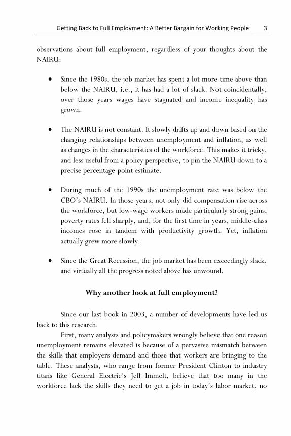
Figure 2-2 shows, between 1949 and 1979 the unemployment rate was
below the NAIRU more than it was above it, to the tune of 15 percentage
points. This implies tight labor markets. A different pattern prevailed post-
1979: Unemployment was 31 percentage points above the NAIRU from 1980
to 2012, though about half of those points are due to the Great Recession. In
the pre-1980 period, the unemployment rate was below the full-employment
benchmark in 84 out of 124 quarters; in the latter period, the unemployment
rate was lower in just 39 out of 132 quarters.
FIGURE 2-2 Cumulative Percentage Points Above or Below NAIRU
Source: Congressional Budget Office and Bureau of Labor Statistics.
What was the impact of those very different labor market regimes on wages
and incomes of working families? Figure 2-3 plots low, middle, and high
incomes, with its 1947 value set to 100. The trends reveal differences in the
nature of income growth over the two periods. When labor markets were
tighter, incomes for these different income classes grew together; when job
markets were slack, incomes grew apart.
-15
31
16
-20
-10
0
10
20
30
40
1949-79 1980-2012 1980-2007

Getting Back to Full Employment: A Better Bargain for Working People 11
FIGURE 2-3 Low, Middle, and High Incomes, 1947-2011
Source: Congressional Budget Office and Bureau of Labor Statistics.
Again, other factors are at play besides the unemployment rate. But
the correlations clearly show income growth, especially middle- and lower-
income growth, is associated with tight labor markets.
Trends in the later 1990s illustrate this point. Figure 2-1 shows that
unemployment stayed below the CBO NAIRU for a number of years during
this period, meaning job markets were tight. This dynamic led to real family-
income growth for all families at all income levels (though the top grew
fastest, meaning inequality continued to increase in these years). Certainly the
factors that economists argue are holding back the income growth of middle-
and low-wage workers, such as globalization and technology, were in play in
those years. Yet strong labor demand created enough pressure to ensure that
low- and middle-wage workers were able to get ahead.
Figure 2-4 shows the results of a statistical exercise to test the
correlation between full employment and trends in real income for different
groups of families. Specifically, the exercise examines the relationship between
changes in real income by income group and the “deviation from full
employment” – movements of the unemployment rate above or below the
full-employment benchmark (see data appendix for more details).4
4 Since the CBOs NAIRU, as shown in Figure 2-1, is fairly constant, this exercise is similar to using the actual unemployment rate rescaled by a constant.
Low
Middle
High
0
50
100
150
200
250
300
3501
947
19
50
19
53
19
56
19
59
19
62
19
65
19
68
19
71
19
74
19
77
19
80
19
83
19
86
19
89
19
92
19
95
19
98
20
01
20
04
20
07
20
10
19
47
=10
0
12 Dean Baker and Jared Bernstein
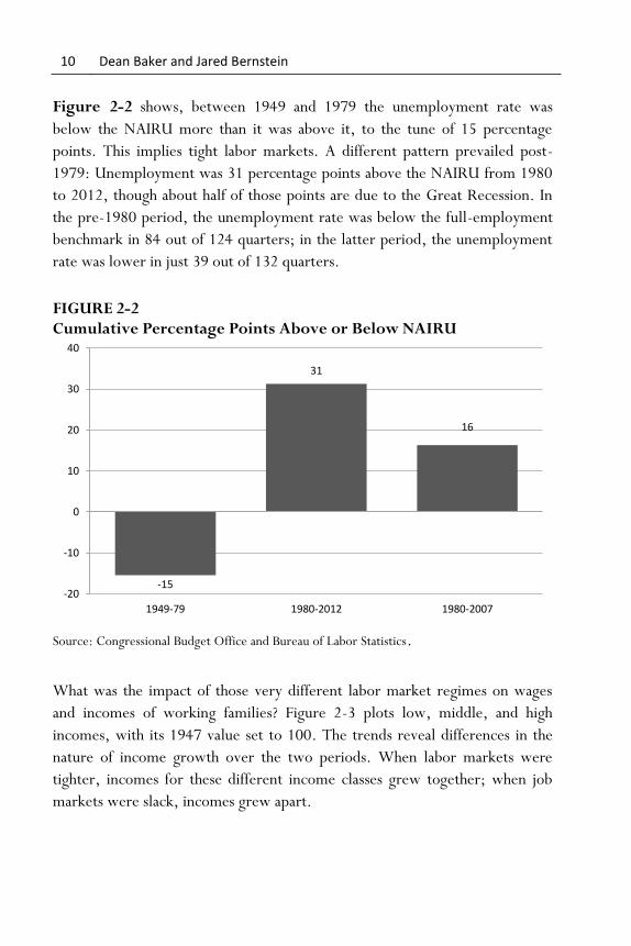
FIGURE 2-4 Impact of Higher Unemployment on Family Income and Inequality
Source: Authors’ analysis of Census, BLS, and CBO data. See appendix for more info.
The pattern of the bars shows that the lower your family income, the
more you lose in slack labor markets. For families in the 20th percentile, for
each percentage point that the unemployment rate was closer to full
employment, incomes grew 2.2 percent.
The correlation was strongest for these families; at the median income
growth was about a third less; and for high-income families (the 95th
percentile) growth was two-thirds less. For African American families the
impact was similar to that for low-income families, and white families saw
gains equivalent to gains at the median.
The last bar is particularly important as it explicitly measures
correlation between slack labor markets and the growth of income inequality,
measured here as the ratio of high to low incomes. One extra point of labor
market slack is associated with a 1.6 percent increase in the ratio of high to
low incomes. Below, we see this same type of relationship in data on earnings,
suggesting an important linkage between slack job markets, uneven wage
gains, and income inequality.
At least for working families, the mechanism upon which these
correlations rest is the paycheck, and that in turn is a result of two important
-2.2%
-1.4%
-0.7%
-1.9%
-1.5%
1.6%
-2.5%
-2.0%
-1.5%
-1.0%
-0.5%
0.0%
0.5%
1.0%
1.5%
2.0%
20thPercentile
Median 95thPercentile
African-American
White 95th/20th

Getting Back to Full Employment: A Better Bargain for Working People 13
factors associated with tighter job markets: more hours of work, and higher
hourly wages. Both are especially important for less-well-off households.
FIGURE 2-5 Annual Hours Worked: Response to 10% Lower Unemployment
Source: Authors’ analysis of U.S. Census Bureau microdata (Annual Social and Economic Supplement) provided by Economic Policy Institute.
Figure 2-5 focuses on annual hours of work among low-, middle-,
and high-income households (summing hours of work across households).
Each bar represents the percent change in annual hours given a 10 percent
change in the unemployment rate.5 The average jobless rate over the period
(1975-2011) was 6.5 percent, so a drop in the unemployment rate to slightly
below 6 percent would raise annual hours for low-income workers by around
2.5 percent. The impact for middle-income workers is about half that, and for
high-income workers about half that again. In other words, the benefits of a
drop in unemployment accrue disproportionately to lower-income families.
This result is an average over the full period. Further analysis looking
specifically at the full-employment years of the late 1990s reveals a particularly
large impact on hours worked by families below the 20th percentile (Figure
2-6). Hours worked were up 17 percent, representing over 100 more hours of
work in 2000 compared to 1996. At high-income levels, hours were virtually
unchanged.
5 The bars in the figures are regression coefficients from regressing the log change in annual hours for each fifth and the log change in the unemployment rate. Each coefficient shown was statistically significant beyond the 0.01 level.
2.4%
1.2%
0.5%
0.0%
0.5%
1.0%
1.5%
2.0%
2.5%
3.0%
Lowest Fifth Middle Fifth Top Fifth

14 Dean Baker and Jared Bernstein
FIGURE 2-6 Change in Annual Hours Worked, 1996-2000, by Income Fifth
Source: Authors’ analysis of U.S. Census Bureau microdata (Annual Social and Economic Supplement) provided by Economic Policy Institute.
Over the comparable period in the 1980s (1985-89), hours for the
bottom group were up only 8 percent, and in the 2000s they were essentially
flat, even as the economy expanded. In other words, full employment
provides the opportunity for the lowest-income workers to expand their labor
supply. Contrary to conservative stories about how low-income people don’t
want to work, these dynamics suggest that given the opportunity, they are the
most eager.
As we undertake this analysis, about 12 million are unemployed and 8
million are working part time but would prefer to be full time. The trends in
these figures underscore how much pent-up labor supply there is in the
country when the economy is poorly managed and the unemployment rate is
high.
We now turn to the impact of unemployment on hourly wages. The
national data used so far are limited both by few observations and the inability
to capture geographical variation. The national unemployment rate is, of
course, an average of jobless rates from across the country, weighted by the
relative size of the local workforce. It is useful to tap that variation across place
and time, as we do here to examine the correlation between unemployment
and real wage growth.
The next set of figures show the results of analyses of the
relationship between the real wages of workers at the 20th, 50th, and 90th
17%
5%
2% 1% 1%
0%
5%
10%
15%
20%
First Quintile Second Quintile Third Quintile Fourth Quintile Fifth Quintile

Getting Back to Full Employment: A Better Bargain for Working People 15
percentiles and the unemployment rates in the state where they live, over the
period from 1979 to 2011. We provide more detail in the technical appendix
to this chapter but for now, the numbers on top of the bars represent the
percent change in real wages with the unemployment rate falls one point.
Across many countries and many time periods, these analyses have shown the
same consistent relationship: Higher unemployment rates mean lower real
wages.6
The patterns here are consistently similar: the less you earn, the more
you need a tight labor market to get ahead. Figure 2-7 shows that a 10
percent decline in unemployment, say from 5 percent to 4.5 percent, is
associated with a 10 percent increase in the real 20th percentile wage, say
from $10 to $11.
FIGURE 2-7 Coefficients on Hourly Wage Variables, Low, Middle and High Wage Workers
Source: Authors’ analysis.
Similar to the relationship we saw in Table 2-1, the wage level’s
responsiveness to unemployment falls as wages get higher, with the effect for
mid-wage workers half that for 10th percentile workers. For wage earners at
the high end of the pay scale, there’s virtually no impact of unemployment on
wage levels.
6 Our regressions follow the recent work of Manchin and Gregg (2012). For a thorough discussion of the theory and extensive empirical research on wage curves, see Blanchflower and Oswald (1995), the canonical reference.
0.098
0.042
0.000 0.000
0.020
0.040
0.060
0.080
0.100
0.120
20th 50th 90th

16 Dean Baker and Jared Bernstein
FIGURE 2-8 Response of Real Wages to Unemployment, by Wage Level and Gender
Source: Authors’ analysis.
Figure 2-8 shows this same relationship by gender. The wages of
low-wage men seem to be more responsive to low unemployment than those
of low-wage women: a 10 percent decline in unemployment is associated with
about a 12 percent increase in men’s real wages and 9 percent for women. The
slightly lower response for women may have something to do with the
minimum wage: The pay of more low-wage women than men is tied to the
minimum wage, and thus the wage floor may be competing with the
unemployment rate as a determinant of the wage level for low-wage women.
Still, the impact of low unemployment is relatively large for low-wage women
workers as well.
Appendix table 2 tests the robustness of these relationships by
examining two other indicators of labor market tightness: the employment
rate and the underemployment rate. These measures both have certain
advantages over the unemployment rate and are thus useful tests of our theory
about the responsiveness of wages to labor market slack. Unlike the
unemployment rate, the employment rate – the share of the 16-year-old and
older population at work – captures the effect of people giving up looking for
work and dropping out of the labor force. Such movements, which have been
0.124
0.038
0.025
0.089
0.042
-0.010 -0.020
0.000
0.020
0.040
0.060
0.080
0.100
0.120
0.140
20th 50th 90th
Men Women

Getting Back to Full Employment: A Better Bargain for Working People 17
common of late, artificially lower the unemployment rate even though they
reflect labor market slack.
The underemployment rate includes various group of underutilized
workers or job seekers who are left out of the official rate (data are only
available since 1994). The largest difference is that the underemployment rate
includes part-time workers who would rather have full-time jobs. Most
recently, there were about 8 million such workers, elevating this measure of
underutilization to around 14 percent compared to about 8 percent for
unemployment (as of the first quarter of 2013). Other components of this rate
include discouraged workers who’ve recently looked for work but given up,
and some other smaller groups that are neither working nor looking for work
but remain marginally attached to the job market.
Both of these alternative measures reveal real wage movements in
response to changing labor market conditions and greater responsiveness
among lower- relative to higher-paid workers. The relationship for lowest-
wage workers suggests that a 10 percent increase in employment rates, say
from 50 to 55 percent, would lead to about a 7 percent increase in the real
wage level of low-wage workers. That impact is five times the magnitude of
that of the highest-paid workers.
The relationship between underemployment and wages follows the
same pattern, but compared with unemployment, the impact is 20-30 percent
greater. This finding suggests that it’s important to look beyond the
unemployment rate to more fully capture the broad dynamics of labor market
slack that are either weighing on or supporting wage growth, particularly as
regards less-advantaged workers.
We can draw two important conclusions from this income, hours, and
wages analysis. First, when the economy operated more frequently at or near
full employment, incomes grew faster and more equally. Other factors were
surely in play, like globalization, that influenced both labor market slack and
wage growth. But the historical record clearly shows two distinct time periods
in which incomes grew together and then apart, and full employment
predominated in only the first period.
Second, the less well-off you are, the more full employment helps
you. Our analysis of hours growth by income class and of high, middle, and

18 Dean Baker and Jared Bernstein
low state-level wages over time finds that low wages and hours worked were
especially responsive to tight labor markets, while the results for high earners
were relatively small and often statistically insignificant. Finally, we found that
underemployment, a more comprehensive measure of slack that includes
persons employed but for fewer hours than they want, is even more highly
correlated with wage levels than is unemployment. This makes it an important
policy target.
A large literature shows other beneficial side effects of tight job
markets. The economist Till von Wachter’s, for example, has focused on
impacts beyond wages, incomes, and hours worked.7
He finds, for example, that long-term unemployment can leave
particularly long-lasting scars, especially for young workers unlucky enough to
begin their careers in a downturn. For these workers, it’s not just that an
initial spell of recession-induced unemployment delays their entry into the job
market. It’s that this delay lowers their “age-wage trajectory” – the extent to
which earnings grow with age – for years to come. Wachter finds that older
workers who lose a stable job can experience earnings declines of 20 percent
lasting 15-20 years.
Moreover, the damage of job loss extends beyond earnings and hours
worked, as job losers have been found more likely to experience a number of
noneconomic negative impacts, including increased rates of stroke and heart
attack, higher rates of divorce, lower rates of home ownership, and even
lower life expectancy. Generational effects have also been found as the
children of parents facing long-term unemployment are more likely to have
lower test scores and reduced earnings as adults than similarly placed children
whose parents avoid long jobless spells.
However one approaches it, when it comes to slack versus tight job
markets, the stakes are high. For that reason, we believe it is essential for
policy makers to chart a course for full employment. The data reveal that the
costs of not doing so are high, especially for those who can least afford them.
Chapters 4-6 suggest a good route.
7 See various publication by von Wachter listed in the references at the end of the book.
Getting Back to Full Employment: A Better Bargain for Working People 19
Chapter 2: Data Appendix
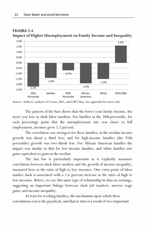
The first table below shows the results plotted in Figure 2.3 in the
chapter. The results are from a time-series regression of the log change in real
family income on the deviation of unemployment from the CBO’s NAIRU
(unemployment-NAIRU for each year), and a trend variable. The table shows
the coefficient on the “deviation from full employment” variable.
TABLE A2-1
Real Income Growth and Full Employment: Coefficients and Related Statistics
Income Group
Coeff t-stat R-sq
20th Percentile -0.022 -8.552 0.632
Median
-0.014 -6.996 0.589
95th Percentile -0.007 -2.402 0.191
African-American
-0.019 -4.622 0.348
White -0.015 -7.839 0.641
95th/20th Percentile
0.016 4.680 0.296
Notes: Coefficients are from regressions of unemployment minus CBO's NAIRU on log real income for the each group. Both variables are entered as first differences and a trend variable is included. The data run from 1949-2011.
Source: Census, BLS, CBO, authors’ analysis.
The rest of the figures and the next table show the results of various
equations which regress workers' real wages on the unemployment rates in the
state where they live, over the period from 1979 to 2011. Economists call
these equations "wage curves" and across many countries and many time
periods, these curves have shown the same consistent relationship: higher
unemployment rates lower wages. The standard wage curves look at the effect
of unemployment on the average wage in the economy. Since we are
interested primarily in the distributional effects of unemployment, we look
instead at the separate effect of the unemployment rate on low-wage workers
(at the 20th percentile of the wage distribution), middle-wage workers (at the
50th percentile), and high-wage workers (the 90th percentile).

20 Dean Baker and Jared Bernstein
We thus have a panel data set of real wages at various deciles along
with state unemployment, underemployment (for a subsample of years), and
employment rates. We regress log wages on the labor market variable, logged
and lagged one period, a specification similar to that of Machin and Greg (see
footnote #7).
TABLE A2-2
Real hourly wages and alternative measures of labor-market slack, 51 States
Employment rate, 1979-2011
Underemployment rate, 1994-2011
20th 50th 90th
20th 50th 90th
Ln(x,t-1) 0.737 0.435 0.144 -0.101 -0.076 -0.044
(s.e.)
0.043 0.048 0.052 0.008 0.008 0.009
Time dummies - - - Not shown - - - - - - Not shown - - -
N
1632 1632 1632 867 867 867
Groups 51 51 51 51 51 51
Notes: Dependent variable is the natural log of the corresponding percentile of the national wage distribution. Ln(x,t-1) is the lagged value of natural log of the employment rate or the underemployment rate. Robust standard errors.

Getting Back to Full Employment: A Better Bargain for Working People 21
Chapter 3
Structural Unemployment: What It Is, Why It Matters, and
Why It’s Not Our Biggest Problem
From the macroeconomic perspective there are three kinds of unemployment – cyclical, frictional, and structural. Economic policy is primarily concerned with cyclical unemployment, which is joblessness due to inadequate demand. Anything that provides a boost to demand, whether it’s more stimulatory fiscal or monetary policy, or increased net exports, should lead to increased employment, so long as workers have the necessary skills and are in the right location for the jobs that are available.
Frictional unemployment is the amount of joblessness due to those who are between jobs. People who are unhappy with their current employers may quit before they have another job lined up, with the expectation that they will be able to find a new job in a relatively short period. This sort of unemployment is not necessarily bad and can even be good, in terms of better, more productive matches between workers and jobs and improved chances of moving up the pay and experience ladder. Frictional unemployment is likely to increase in a healthy labor market, since workers will be more likely to leave a job without having another one arranged if they think it will be easy to find a new job.
Younger workers are more likely than older, experienced workers to be frictionally unemployed. People in their teens and twenties are unlikely to have lengthy experience with a single employer, which means that they give up less in terms of seniority and earned benefits if they quit their jobs. They are also less likely to be tied down with family obligations and mortgage payments, and thus freer to go a period of time without a paycheck or to move across town or across country. For these reasons, frictional unemployment was likely to be much larger in the 1970s and 1980s, when the huge baby boom cohorts made the labor force relatively young, than it would be today, when the baby boomers are in their 50s and 60s. A lower level of frictional

22 Dean Baker and Jared Bernstein
unemployment might be a good reason to expect lower overall unemployment today, if the economy were not in a slump.
Frictional unemployment can be loosely measured by the percentage of unemployment that is due to “job leavers,” or people who are unemployed after voluntarily quitting their jobs. The match is not precise, because frictional unemployment includes other categories of unemployed workers as well, such as people just entering the labor force after leaving school or re-entering the labor force after caring for a child or relative. But the number of unemployed job leavers should give a reasonable approximation. In periods when the labor market was relatively healthy, as in 2007 and 2000, job leavers accounted for 11 and 13 percent of total unemployment, respectively. This share fell sharply in the downturn, to a low of 5.6 percent in June 2009.8
As a practical matter it would be desirable to minimize the time that workers have to spend looking for jobs, since it is a loss to both the unemployed worker and the economy as a whole.
Finally, structural unemployment is joblessness that results from a mismatch between the skills employers demand and the skills that workers have to offer. It cannot be eliminated through increased demand. It is crucial to understand and estimate structural unemployment, because (in combination with frictional unemployment) it represents the floor in our pursuit of full employment.
It is not easy to determine where cyclical unemployment ends and structural unemployment begins, but there are features of the labor market that indicate which type of unemployment is afflicting the economy. First of all, if most unemployment is structural, then you would expect to see a significant and persistent gap between the type of workers that employers need and the type of workers that are unemployed. Unlike in the cyclical case, in the structural case there is plenty of demand, but the unemployed don’t have the right skill sets to meet employers’ needs.
It may seem intuitive that one way to learn about the extent of structural unemployment is to just listen to employers when they say they can’t find enough workers with the skills required by their job openings. But employers often make this complaint, even when unemployment is high for
8 Since unemployment was more than twice as high in 2009 as in 2000 or 2007, the percentage of the labor force who were unemployed as a result of quitting their jobs changed much less dramatically.

Getting Back to Full Employment: A Better Bargain for Working People 23
highly educated workers, so we need more reliable signals by which to gauge structural unemployment. Fortunately, there are three.
The first is rising pay. When shortages exist in occupations or areas, wages should rise rapidly as firms bid up the price of available labor. To provide a good measure of whether such shortages are afflicting the economy generally, the sectors have to be large in order to have a substantial impact on employment. There will always be narrow areas involving highly specialized skills in which workers are in high demand. For example, some types of computer scientists will likely be in high demand even in the steepest downturns, but a tiny sector that currently employs 10,000-20,000 people will not make much of a dent in re-employing the millions laid off in manufacturing or construction. Establishing a problem of structural unemployment means finding large areas in which workers with the necessary skills are in short supply and wages are being bid up rapidly.
The same challenge applies when examining compensation and locational mismatches. It is always possible to identify labor markets of limited size where there may be shortages of labor. For example, North Dakota maintained an unemployment rate of 4.0 percent even in the worst years of the Great Recession. Workers in the state experienced substantial pay increases – the average weekly wage rose 16 percentage points more than the national average from 2007 to 2011.9 Clearly more workers could have been employed if they had opted to move from areas of high unemployment to North Dakota. However, the economy-wide impact of a mass migration to North Dakota would have been minimal. In 2011 there were 380,000 people employed in North Dakota. Boosting that number by a massive 25 percent would reduce the national unemployment rate by less than 0.1 percentage point. To make a serious case that a mismatch between the location of unemployed workers and the location of the available jobs is a major cause of unemployment would require identifying dozens of North Dakotas.
A second way to gauge whether we are dealing with structural unemployment is to determine whether the average workweek is getting longer. If a company has job openings for which it is unable to find qualified workers, yet customers are clamoring for its products, then the company’s
9 Data on wage growth for North Dakota are taken from the Bureau of Labor Statistics Quarterly Census of Employment and Wages. The national wage data are taken from the Current Employment Statistics Survey.
24 Dean Baker and Jared Bernstein
natural response would be to work the existing workforce more hours. If structural unemployment is explaining a substantial portion of the unemployment in the economy, then we should see a rise in hours in large sectors of the economy, not just in a few narrow industries and occupations.
A third feature of an economy that is experiencing structural unemployment should be a rise in the ratio of job openings to unemployed workers. This would suggest that firms are finding it difficult to get workers with the necessary skills.
Looking at these three criteria, it seems clear that the United States in 2011-12 was suffering overwhelmingly from cyclical, not structural, unemployment. Overall wage growth over this period was at best keeping pace with inflation, and one would look in vain for any major occupation or industry group in which wages were rising rapidly. The length of the average workweek was approaching pre-recession levels in many sectors, but there were no major sectors where the workweek appeared to be rising much above that.
The ratio of job openings to unemployed workers ticked up slightly in 2011-12, but there are explanations for this trend unrelated to structural unemployment. A paper by the Boston Federal Reserve Bank (Ghayad and Dickens 2012) found that the rise in the ratio of job openings to unemployed was entirely due to a rise in the ratio of job openings to long-term unemployed. The paper found that the ratio of job openings to short-term unemployed (less than six months) continued to follow its usual pattern. This means that any mismatch suggested by the rise in this ratio is occurring only among the long-term unemployed. There are several possible explanations for this pattern.10 It could be the case that employers are discriminating against workers who have been unemployed for long periods (Kroft, Lange, and Notowidigdo 2012).11 In a period of lower unemployment this may not be an option, but in a
10 The temptation to say that the long-term unemployed are the ones who lack skills doesn’t fit the data. The long-term unemployed had at one time been among the short-term unemployed. If this group is especially ill-fitted to the current job market, then they should have also been driving up the ratio of short-term unemployment to vacancies.
11 In a subsequent paper Ghayad (2013) examined this issue. He sent out resumes showing workers who had been unemployed for different periods of time but were otherwise identical. The resumes showing short periods of unemployment often received invitations for interviews, but employers almost never arranged for interviews with the long-term unemployed.

Getting Back to Full Employment: A Better Bargain for Working People 25
prolonged period of high unemployment, employers can afford to be selective about whom they hire. There is also likely to be less urgency about hiring in a downturn, since the company is probably not fully utilizing its existing workforce (Davis, Faberman, and Haltiwanger 2013).
It could also be the case that workers are being more selective about the jobs they are willing to accept. Due to the severity of the downturn, the duration of unemployment benefits has been considerably longer in this downturn than in prior postwar recessions. As a result, the long-term unemployed are far more likely to still be collecting benefits than would otherwise be the case, taking advantage of the opportunity to wait longer to find a job that fully utilizes their skills. Recent research has found a limited amount of evidence that the increased duration of benefits has caused people to be unemployed somewhat longer, although this effect does not appear to be large (see Rothstein 2011; Daly et al. 2011). At the point where unemployed workers are no longer eligible for benefits, most give up looking for work and drop out of the labor force; they do not suddenly find jobs. Given this pattern, the main way in which longer benefits lead to a higher unemployment rate is by keeping people in the labor force looking for jobs and therefore counted as unemployed (you must be looking for work to be counted as unemployed and to qualify for benefits). It does not appear that the longer period of benefit duration has caused large numbers of workers to turn down jobs they would have otherwise accepted.
Presumably the cause of the rise in the ratio of job openings to the number of long-term unemployed is some mix between changes in employer behavior and workers’ behavior. However, the fact that the rise in the ratio does not appear among the short-term unemployed suggests that the problem is not one of a general skills mismatch.
It’s also a mistake to jump from the observation of job openings to the assumption that employer labor demands are not being met. Posted job openings do not always signal actual labor demand; they may represent employers “testing the waters” by offering below-market wages (Rothstein 2012). 12 One therefore needs to see whether industries with lots of job openings are actually growing and/or offering higher wages. If this correlation is close to zero (which Rothstein finds to be the case in recent years), then there is probably little connection between increased openings and actual job creation.
12 See discussion regarding Figure 10 on page 15.
26 Dean Baker and Jared Bernstein
There is one other point worth making on the concept of structural unemployment: As Mark Thoma has frequently pointed out in his blog, Economist’s View, unemployment that appears to be structural in the context of a depressed economy may prove to be cyclical if the economy were to return to full employment (Thoma 2011). For example, the wages being offered during the downturn in a relatively prosperous area may not be sufficient to induce workers to move from areas of higher unemployment. However, when the economy gets closer to full employment, employers in prosperous areas might be willing to offer higher pay, thereby providing the incentive necessary to get workers to move from pockets of high unemployment. The same could be said of skills acquisition, where workers may need a slightly higher wage in order for them to have the incentive necessary to develop skills for specific jobs. During a downturn employers may not offer a high enough wage for workers to spend the time and money necessary to acquire these skills, but in a stronger economy wages may rise to the point where either workers or employers make the necessary investment.
The boom of the late 1990s provided examples of both developments. Businesses located in suburban areas reportedly chartered buses to make it easier for workers from the inner cities to work at jobs in hotels, restaurants, and other relatively low-paying sectors, and employers found ways to hire workers with various types of disabilities for these jobs (Uchitelle 2000). The Atlanta Federal Reserve Bank reported in December 1999 that firms were hiring less-experienced workers than they would typically and training them for open jobs (Federal Reserve Board 1999). Firms in Omaha, Neb. offered in-house child care and even elder care in order to attract and retain workers (Omaha World-Herald 1999).
In a weaker labor market, it would not have been profitable to incur these additional expenses. However, the strength of the late 1990s economy made it profitable for firms to take unusual steps to get additional labor. As a result, the unemployment rate fell to a year-round average of 4.0 percent in 2000, a level far lower than what almost all economists had considered possible just five years earlier.
These anecdotes actually amount to a powerful insight regarding social policy. The government spends considerable resources to train and employ disadvantaged workers, with middling success. 13 Full employment
13 For a useful review, see Harry Holzer, Workforce Development Programs, 2013.

Getting Back to Full Employment: A Better Bargain for Working People 27
accomplishes this same goal organically through the private market and at no cost to government coffers. In fact, as we note in Chapter 4, full employment is a strong revenue-positive fiscal policy.
The rise in the estimated structural-unemployment rate
The view of policymakers, and in particular the Federal Reserve, on
the level of structural unemployment in the economy is important, since this measure provides an implicit policy target. The Fed would not be interested in trying to further stimulate the economy if it viewed the remaining unemployment as structural. The level of structural unemployment is also important for budgetary purposes. Long-term budget projections from the Congressional Budget Office, the Office of Management and Budget, and other official forecasters typically assume that the unemployment rate will hover near the level of structural unemployment. The estimate provides the basis for revenue and spending projections. (This issue is examined in more detail in Chapter 4.)
In principle, if the unemployment rate has fallen to the level where the remaining unemployment is primarily frictional and structural, then it makes little sense to try to boost demand to further reduce the unemployment rate. In this view, any additional boost to demand may temporarily lower unemployment, but only at the cost of raising inflation. Since in this scenario those who are unemployed are not willing to work at a wage that is consistent with their level of productivity, they can only be persuaded to work if inflation deceives them about the value of their wage. If they are offered a higher nominal wage, but fail to recognize that prices are rising more rapidly, then workers can be tricked into working for a lower real wage.
However, this policy would be of limited value in lowering the unemployment rate. First, it can only work as long as workers can be deceived about the real value of their wage. If they anticipate 2.0 percent inflation and then realize the inflation rate is actually 3.0 percent (i.e., they find their paycheck doesn’t go as far as they expected in the “real” world), then it will take a 4 percent or even 5 percent inflation rate to trick these workers into accepting a lower real wage. In this story, inflation would have to be continually accelerating to maintain an unemployment rate below the structural rate of unemployment.
The other problem of pursuing an unemployment rate that is below the structural rate in this context is that it is not clear that it actually is doing

28 Dean Baker and Jared Bernstein
anyone a favor. In this story, workers always had the opportunity to work if they were willing to accept a lower real wage that reflected their actual productivity. They opted instead not to work at this wage, effectively making their unemployment voluntary. The unexpected rise in the inflation rate persuades them to work for a real wage that is so low that they would rather not be working. In this case, the low unemployment policy simply tricked people into working for a lower real wage than they considered acceptable.
For these reasons, if we can accurately identify structural (and frictional) unemployment, it does not make sense to pursue macroeconomic policies that push the unemployment rate lower. Any effort to do so will result in higher inflation and will not really benefit the workers who were employed as a result. This is the concept of the non-accelerating inflation rate of unemployment, or NAIRU, which is supposed to be the rate of unemployment that is consistent with a stable rate of inflation.
As a practical matter, economists have not been very successful in their efforts to determine the NAIRU. In the early and mid-1990s the economics profession was nearly unanimous in its view that the structural rate of unemployment was close to 6.0 percent (Krugman 1995; Weiner 1993; Gordon 1988; Brauer 2007), and the Federal Reserve began raising interest rates in the winter of 1994 based on that estimate. The unemployment rate was falling rapidly toward 6.0 percent, which was in the middle of the range of estimates of the NAIRU. In order to limit the economy’s growth and to prevent the unemployment rate from continuing to drop, the Fed raised the interest rate on overnight money from 3.0 percent in February 1994 to 6.0 percent by February 1995. The rate hikes had the intended effect of slowing the economy and limiting the decline in the unemployment rate.
However, in the summer of 1995 then-Federal Reserve Board Chairman Alan Greenspan made a remarkable break with the orthodoxy within the profession. He insisted that he saw no evidence of inflation in spite of the fact that the unemployment rate, at 5.7 percent, was below the conventional range of estimates for the structural rate of unemployment. As a result, he pushed through a cut in interest rates that opened the door for a speedup of the economy and further declines in the unemployment rate. By the summer of 1997 the unemployment rate had fallen below 5.0 percent. It fell below 4.5 percent the following summer and finally stabilized near 4.0 percent, the year-round average for 2000.
Through most of this period there was no evidence of any substantial uptick in the rate of inflation, but in 2000 it began to increase, rising at a 3.0

Getting Back to Full Employment: A Better Bargain for Working People 29
to 3.5 percent annual rate for much of the year, compared to under 2.0 percent in 1998. However, even this increase was largely the result of an uptick in world energy prices that could not be attributed to the low unemployment rate in the United States. The core inflation rate in 2000 was 2.4 percent, essentially the same as the 2.3 percent rate in 1998 and only slightly higher than the 2.1 percent rate in 1999. While it can be argued that the 4.0 percent unemployment rate was in fact below the economy’s structural unemployment rate, and therefore leading to limited inflationary pressure, the evidence from this period suggests that the true structural rate of unemployment was well below the range of estimates that were widely accepted in the economics profession in the middle of the decade.
Had Alan Greenspan not been an eclectic economist who was willing to challenge economic orthodoxy, we might never have had the 1990s experiment with low unemployment. If he followed the script as his colleagues urged, he would have raised interest rates enough in 1995 and 1996 to keep the unemployment rate from dropping below the range of estimates for the structural rate of unemployment. This policy would have denied millions of people the opportunity to work in these years, and prevented the widely shared wage gains that were made possible by the strength of the labor market. And it would have prevented the world from recognizing that the economics profession was wrong, since its estimate of the structural rate of unemployment would otherwise never have been tested.14
As the unemployment rate falls in the years ahead we will face similar controversies. Indeed, prominent voices in the profession claim that the unemployment rates we are now seeing are consistent with the structural rate of unemployment in the economy.15 From this perspective, efforts by the Fed
14 There is a peculiar asymmetry in testing economic policies. If believers in a high NAIRU control policy, then we will never be able to directly test if they are wrong because they will not allow the unemployment rate to fall below their estimate of the NAIRU. On the other hand, if believers in a lower NAIRU control policy, then they will allow the unemployment rate to fall, providing a direct test of whether their view of the NAIRU was correct.
15 Minneapolis Fed President Narayana Kocherlakota has perhaps been the most prominent proponent of the view that the high unemployment seen in the downturn is primarily structural (see, e.g., his “Inside the FOMC” speech from summer 2010), but many other economists have made this case, as have Richard Fisher, the former president of the Dallas Fed, and Charles Plosser, the president of the Philadelphia Fed. To Kocherlakota’s credit, he reversed his position in the summer of 2012 when the course of the recovery did not
30 Dean Baker and Jared Bernstein
to boost the economy with low interest rates and quantitative easing, or by Congress to use spending and tax cuts to increase demand, are foolhardy, since they will primarily have the effect of raising the inflation rate while having little impact on output and employment.
Their argument is that the downturn represents a fundamental shift in the economy. In their view, the bursting of the housing bubble left a huge pool of workers with capabilities in construction and manufacturing; when the economy recovers we are not likely to see as much employment in these sectors as before, and so millions of former construction and manufacturing workers will be structurally unemployed.16
While this is a minority view in the profession, as evidenced in part by the fact that the Fed’s Open Market Committee has overwhelmingly supported expansionary policy, more moderate voices have argued that the NAIRU is considerably higher than it was before the downturn. For example, CBO has raised its estimate of the NAIRU for the later years in this decade by 0.7 percentage points, from an estimate of 4.8 percent in January 2008 (CBO 2008) at the beginning of the downturn to 5.5 percent in its latest economic projections (CBO 2012). After a meeting of the Fed’s Open Market Committee In June 2013, Fed Chairman Ben Bernanke indicated that he considers full employment to be in the range of 5.5 to 6.0 percent.
This increase in the estimate of the NAIRU will have substantial consequences if it becomes the basis for policy. Just as the Fed would have placed a floor on the unemployment rate of close to 6.0 percent in the mid-1990s if it had followed the orthodoxy within the profession at the time, it could also put a floor on the unemployment rate of 5.2 percent or higher later
appear consistent with his view that unemployment was structural rather than cyclical (Hilsenrath 2012).
16 A strong argument against this view is that the unemployment rate for workers in the manufacturing sector was actually lower than the overall unemployment rate in 2012 – 7. 3 percent for workers in manufacturing compared to 8.1 percent overall. At 13.9 percent, the unemployment rate for workers in the construction industry was still higher than the overall average, but this was the case before the downturn – the unemployment rate for construction workers in the three years preceding the downturn had been on average more than 2.0 percentage points higher than the overall unemployment rate. This means that the gap between the unemployment rate of construction workers and the overall unemployment rate grew by less than 4.0 percentage points during the downturn, an amount that would explain a rise in the overall unemployment rate of less than 0.2 percentage points.
Getting Back to Full Employment: A Better Bargain for Working People 31
in the decade when the economy may finally have recovered from the effects of the recession. If the unemployment rate could in fact fall to 4.0 percent, and possibly lower, without leading to accelerating inflation, then the result of a policy that kept it higher would be the needless unemployment of millions of workers and lower wages for tens of millions. The rise from a target unemployment rate of 4.8 percent to just 5.2 percent would mean the loss of more than 1 million jobs.
Unemployment targets through 2020
Because the track records of the Federal Reserve and the economics
profession in identifying the NAIRU have been consistently poor, monetary and fiscal policy should err on the side of low unemployment and aim to push the unemployment rate as low as possible. The reason for this is simple: The costs of pushing too far – allowing the unemployment rate to fall so low that it leads to a rise in the rate of inflation – are much smaller than the costs of erring on the other side, which include denying employment to people who would otherwise have jobs in a fully employed economy. Erring on the side of excessive unemployment also means denying wage growth to tens of millions of workers in the bottom half of the wage distribution, thereby continuing the upward redistribution of income we have seen over the last three decades.
We are not making an argument about an actual tradeoff between rates of inflation and unemployment, a case that was sometimes made in the 1960s. The issue is one of relative risks. We understand that as the unemployment rate falls to lower levels, the risk of accelerating inflation increases. But if the rate of inflation is not accelerating, there is the risk that people are being needlessly denied the chance to work and wages for those at the bottom are being held down by bad government policy. Based on the relative costs, it seems far better to take the risk of a short period with rising inflation than maintaining a higher-than-necessary level of unemployment.17
While it has arguably always been the case that it is better policy to err on the side of less unemployment, new research suggests that the cost
17 In the language of the Federal Reserve, the target on the price side of the unemployment/inflation tradeoff is not just the rate of inflation, but inflation expectations: the rate at which people expect inflation to increase or fall in the future. This is important because, if people and businesses expect inflation to remain stable, they’re less likely to react to a temporary up-or-down spike.
32 Dean Baker and Jared Bernstein
asymmetry is even greater today. A recent study by the Congressional Budget Office (Arnold 2008) found that in the last decade the relationship between increases in inflation and unemployment have become weaker statistically, and the terms of the tradeoff have become more favorable. The first point means that we have less reason than we had in the past to believe that low rates of unemployment will necessarily lead to higher rates of inflation.18
The second point is that the cost in terms of higher inflation of being below the NAIRU is less than was previously the case. Prior research has suggested a tradeoff of roughly a 0.5 percentage-point increase in the rate of inflation with an unemployment rate that was a full percentage point below the NAIRU for an entire year. So if the NAIRU was in fact 5.0 percent, but we pursued an expansionary policy that allowed the rate of unemployment to fall to 4.0 percent, then the rate of inflation, had it been, say, 2.0 percent, after a year would be 2.5 percent. The new research suggests a tradeoff of just 0.3 percentage points after a year. Of course, the theory still implies that inflation will continue to rise as we sustain the unemployment rate a full point below the NAIRU, but, if we take steps to slow the economy and raise the unemployment rate back to the NAIRU, we could prevent any further rise and allow the inflation rate to stabilize at 2.3 percent instead of the prior 2.0 percent.
If 2.0 percent is indeed the optimal rate of inflation, there will be some economic consequences of living with a 2.3 percent rate. But they have to be weighed against the benefits of giving another 2 million people jobs and allowing for considerably more rapid real wage growth for the bottom half of the labor market. Given the large degree of uncertainty in the estimation of the NAIRU, there seems no justification for not trying to push down the unemployment rate as low as possible until there is clear evidence that labor market tightness is causing inflation.
18 Interestingly, the Chow tests in this paper to determine whether there was a break in the relationship between inflation and the unemployment rate find the strongest evidence for a break at the end of the 1980s. If this result accurately reflects the actual relationship between inflation and unemployment, then the economy already had the potential to have a lower unemployment rate without accelerating inflation by the early 1990s, several years before the productivity pickup in the middle of the decade and other changes that were at the time dubbed the “new economy.” If such was the case, then the Fed needlessly kept the unemployment rate high with its hesitance to lower interest rates following the 1990-91 recession and then by raising rates in 1993-94 to keep the unemployment rate from falling below the level it perceived as the NAIRU.
Getting Back to Full Employment: A Better Bargain for Working People 33
The logic of the 2.0 percent inflation target
The central banks that control monetary policy in most wealthy
countries have adopted a 2.0 percent inflation target as their main or only goal in the conduct of monetary policy. If a central bank fervently sticks to this goal, it will ignore all other considerations, such as the rate of growth of the economy, the level of unemployment, or even the prospective collapse of the financial system, to focus on maintaining the 2.0 percent inflation target.
As a practical matter, there is probably no central bank that would place a greater priority on its 2.0 percent inflation target than on preventing the collapse of the financial system, but the stated and often legal commitment of central banks across the globe is to this 2.0 percent target. The European Central Bank has this commitment in its charter, and it is the official target for policy of the Bank of England. The Federal Reserve under Ben Bernanke is ostensibly committed to a 2.0 percent inflation target, even though its mandate from Congress requires it to pursue both price stability and high employment.19 Given the rapid spread of inflation targeting as the basis for central bank policy, it is worth asking where this urge originated.
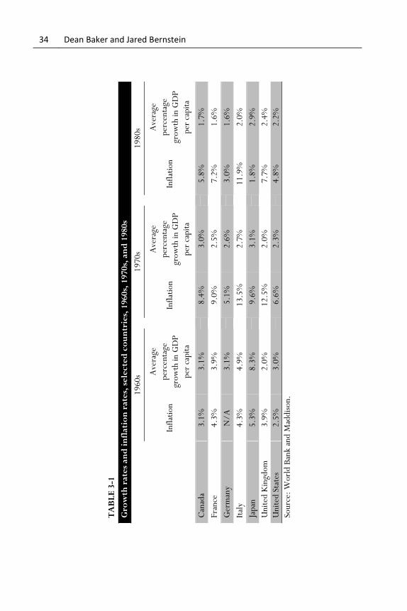
First, note that wealthy countries have generally had inflation rates well above 2.0 percent and still managed to maintain healthy growth rates. Table 3-1 shows the average inflation rate and the average growth rate for the 1960s, 1970s, and 1980s for seven developed countries, including the United States. Most of these countries had inflation rates that averaged well above 2.0 percent in each of these decades yet still maintained strong real growth. Clearly the 2.0 percent inflation target is not essential for maintaining growth.
There are two lines of argument for the 2.0 percent inflation target. The first has to do with distortions, many of them due to the tax code, that result from inflation. The logic is fairly straightforward: If there is inflation, then what may appear to be profits or income are really the result of prices keeping pace with inflation. If a company sells its output at the end of the year for prices that are 5 percent higher than what it received the prior year, and there is 5 percent inflation, then the company made zero real profit.
19 In response to the downturn, the Fed has also set unemployment targets for the timing of reversing its expansionary policies. It is not clear whether explicit unemployment targets will play a role in Fed policy if the unemployment rate returns to more normal levels.
34 Dean Baker and Jared Bernstein
TA
BL
E 3
-1
Gro
wth
rat
es
and
in
flat
ion
rat
es,
se
lec
ted
co
un
trie
s, 1
960
s, 1
970s
, an
d 1
980s
1980
s Ave
rage
perc
enta
ge
grow
th in
GD
P
per
capi
ta
1.7%
1.6%
1.6%
2.0%
2.9%
2.4%
2.2%
Sour
ce:
Wor
ld B
ank
and
Mad
diso
n.
Infl
atio
n
5.8%
7.2%
3.0%
11.9
%
1.8%
7.7%
4.8%
1970
s Ave
rage
perc
enta
ge
grow
th in
GD
P
per
capi
ta
3.0%
2.5%
2.6%
2.7%
3.1%
2.0%
2.3%
Infl
atio
n
8.4%
9.0%
5.1%
13.5
%
9.6%
12.5
%
6.6%
1960
s Ave
rage
perc
enta
ge
grow
th in
GD
P
per
capi
ta
3.1%
3.9%
3.1%
4.9%
8.3%
2.0%
3.0%
Infl
atio
n
3.1%
4.3%
N/
A
4.3%
5.3%
3.9%
2.5%
Can
ada
Fran
ce
Ger
man
y
Ital
y
Japa
n
Uni
ted
Kin
gdom
Uni
ted
Stat
es

Getting Back to Full Employment: A Better Bargain for Working People 35
But if we don’t recognize the effect of inflation in the tax code, we tax companies on profits that do not exist.20 The same applies to the treatment of capital gains. Numerous studies have sought to measure the size of the distortions that result from even modest rates of inflation. Many have found these costs to be substantial, on the order of 1.0 percent of GDP for an inflation rate of just 1.0 percent (see e.g. Feldstein 1997; Fisher 1981).21
While these studies present static costs – such as costs that are due to an ongoing distortion in the tax system – there are also studies that purport to show dynamic costs, meaning that the rate of growth will be slower as a result of higher rates of inflation. In principle dynamic costs are likely to be of more consequence than static costs because they grow over time. For example, if a higher inflation rate slows growth by 0.1 percentage point annually, then after 10 years GDP will be 1.0 percent less than it would have been with a lower rate of inflation. After 20 years it would be 2.0 percent less. These costs will continue to rise over time, so that even a relatively small difference in growth rates will eventually produce a large loss of GDP. As a result, economists view the potential impact of inflation on growth as enormously important.
Numerous studies have examined the link between inflation and growth. Many have found that the link is weak or nonexistent (e.g. Bruno and Easterly 1998; Grier and Tullock 1989; and Levine and Zervos 1993), but a number have found a significant negative relationship between even modest rates of inflation and GDP growth.22 For example, Grimes (1991) looked at 21
20 It is in principle possible to adjust the tax system to reduce the distortionary impact of inflation – for example, by adjusting the cost basis for sales from inventories to their replacement cost. However, this adjustment can never be made perfectly.
21 It is worth noting that distortions from the effect of inflation on tax liability can be reduced through changes to the tax code. If capital gains are indexed in some way to inflation, then the deadweight loss from the effect of inflation on taxes can be substantially reduced, as would be the case with interest or dividend payments. Indexation raises complications, but it is an option if the distortions from inflation are felt to be sufficiently serious.
22 It is important to emphasize that the debate is over the relationship between growth and low to moderate rates of inflation, in the neighborhood of 3-6 percent, not rates of 30 or 40 percent. While there are plenty of examples of countries that have maintained healthy growth rates even with double-digit inflation rates, it is fair to say that such rates raise a qualitatively different set of questions than the inflation rates that may arise from having an unemployment rate that is 0.5 to 1.0 percentage points below the level that is consistent with stable inflation for a period of time.

36 Dean Baker and Jared Bernstein
countries in the Organization for Economic Cooperation and Development over the period from 1961 to 1988 and found that a 1.0 percentage-point increase in inflation was associated with a 0.11 percentage-point drop in the growth rate. Fischer (1993) had comparable results examining a group of non-oil-exporting countries over the same period. Looking at a sample of more than 80 countries over the years 1960 to 1990, Barro (1995) found that a 1.0 percentage-point rise in the inflation rate was associated with just a 0.02 percentage-point decline in the growth rate.
Proponents of a 2.0 percent inflation target argue that the studies showing even modest rates of inflation reducing growth are sufficiently conclusive that central banks should adopt their inflation target as the basis of policy.23 For example, Anderson and Gruen (1995) reviewed 15 studies of the relationship between inflation and growth, and nine of them found a relationship (significance level of at least 10 percent) between inflation and slower growth. Based on this evidence, and the fact that none of the studies found a significant positive relationship between inflation and growth, the paper concludes that even modest rates of inflation will slow growth.
But skeptics have raised two important points about this literature on the link between inflation and growth. The first is that we essentially have a mixed set of findings. Why is it clearly possible to structure studies in ways that find a negative relationship and to structure others that find no relationship? Looking at the mixed track record it is far from obvious that the weight of evidence is strongly in a negative direction.24 Usually when there is a strong relationship between two variables – such as that claimed to be the case between inflation and growth – it is difficult to structure a test that does not find a link.
23 In fairness to advocates of inflation targeting, there is a wide range of views as to how strictly we should hold to the target as the primary or only goal of monetary policy.
24 There is also the possibility of publication bias. Given the strong belief by many economists that inflation reduces growth, there may be a reluctance to publish articles that find either insignificant results or even a positive relationship. This sort of publication bias was noted in the case of the minimum wage, where the distribution of published results has an otherwise inexplicable break at zero. If we assume that study results are normally distributed, there should be some number of studies that find a significant positive relationship between higher minimum wages and employment even if the true coefficient for an employment variable is zero (Doucouliagos and Stanley 2009).

Getting Back to Full Employment: A Better Bargain for Working People 37
Even if the weight of the evidence from published studies can be viewed as supporting the case that there is a relationship between moderate rates of inflation and slower growth, there are still grounds for questioning the findings. For example, it will in general be the case that supply shocks will push inflation and growth in opposite directions. If a crop failure pushes up the price of a major food product, or a cutoff in energy supplies leads to higher gas and electricity prices, then we would expect to see both slower growth and higher inflation. The same is true in the opposite direction. If a huge new energy source comes on line, or a major innovation raises productivity growth and reduces the cost of production, we would expect to see both lower inflation and an increase in output. For these reasons, any sort of simple look at the correlation between inflation and growth rates would likely find that higher inflation is associated with slower growth.
Of course, the studies that attempt to measure the relationship between inflation and growth are carefully done and try to control for these sorts of supply shocks, thereby removing their impact. However, it is never possible to perfectly control for all the shocks that may affect an economy. It might be relatively easy to identify surges in food or oil prices, but other factors may be harder to identify. For example, a labor disruption that slows production and raises costs may not be picked up in these sorts of studies, since doing so requires an intimate knowledge of the history of the country included in the analysis. Insofar as the analysis misses the impact of supply shocks in either direction, there will be a bias toward finding that higher inflation slows growth even if there is in fact no relationship. For this reason, some view this literature as being less conclusive than the proponents of inflation targeting believe.
Skeptics also question the rationale for a 2.0 percent inflation target as opposed to a 0.0 percent target. Advocates of the 2.0 percent target generally take the view that 2.0 percent measured inflation corresponds to 0.0 percent actual inflation, based on their belief that inflation is measured with a high-side bias. They argue that official measures of inflation like the consumer price index fail to pick up the benefits of new products and various quality improvements; they adjust for this by assuming that an official inflation rate of 2.0 percent means that actual inflation is close to zero (see e.g. Feldstein 1997).
However, this assumption raises a fundamental problem with the sort of studies that the proponents of inflation targeting use as evidence to support this policy. If there is a large error in the measure of inflation, then this

38 Dean Baker and Jared Bernstein
measurement error is likely to cause these studies to find a negative relationship between inflation and growth even if there is no such relationship.
To see this point, it is important to remember that real GDP growth is equal to nominal GDP growth minus the rate of inflation:
Real GDP growth = nominal GDP growth – inflation
So if nominal GDP grows by 5.0 percent and the inflation rate is 2.0
percent, then real GDP growth is 3.0 percent. But proponents of inflation targeting argue that the measured rate of inflation is subject to a large amount of error, so that 2.0 percent measured inflation may actually correspond to zero inflation. This means that measured GDP growth will be equal to nominal GDP growth minus the true rate of inflation and the error in the measured rate of inflation:
Measured real GDP growth = nominal GDP growth – (true inflation + error in measure of inflation)
This creates a serious problem for economists trying to measure the
relationship between inflation and GDP growth. Any upward bias in the measured rate of inflation will lead to both higher measured inflation and lower measured growth. This would mean that even if there is no relationship whatsoever between inflation and GDP growth, regression analysis would likely find a negative relationship (higher inflation, slower growth) for the simple reason that countries that have less error in their measure of inflation would also show stronger growth.
To take a simple example, suppose two countries both actually have 5.0 percent real GDP growth and 0.0 percent inflation. In other words, if we could look at these countries from the standpoint of an all-knowing observer who always got prices and quantities right, we would be able to see that GDP was growing at a 5.0 percent rate in both countries and there was no inflation. Now suppose that country A has a somewhat more accurate price index than country B (although both are slightly off). The index in country A shows an inflation rate of 1.5 percent, while the index in country B shows an inflation rate of 2.0 percent. In this scenario, the measured growth rate for country A would be 3.5 percent, and the measured growth rate for country B would be just 3.0 percent. So if we were looking at these two countries from the standpoint of the measured data, as opposed to the all-knowing observer, we

Getting Back to Full Employment: A Better Bargain for Working People 39
would think that country A had both lower inflation and higher growth than country B. It is difficult to see a way around this sort of problem in measurement.25 If it is the case that our inflation data contain substantial error, as proponents of a 2.0 percent inflation target argue, then it means that differences in the amount of measurement error across countries could drive the result that many studies find. Unless we make the assumption that the error in the measurement of inflation is constant across countries and through time, then there seems no way to avoid the conclusion that measurement error could explain the results of analyses tying higher inflation to lower growth. Given the large differences in the methodology used to measure inflation across countries (even taking into account efforts to harmonize price indices in recent years), the assumption that the measurement error is the same across countries and through time is not plausible.
The size of the estimated impact of inflation on growth in the studies that found an effect is certainly well within the range that could be explained by measurement error. The range of significant coefficients in the collection of studies by Anderson and Gruen ranges from 0.024 percent to 0.2 percent. Even the higher end of this range is well within the plausible differences in the measurement of the rate of inflation across countries and through time. For example, the Council of Economic Advisers estimated in 1999 that changes in methodology used to construct the consumer price index in the years from 1995 to 2000 would lower the measured rate of annual inflation by 0.68 percentage points (CEA 1999, 94). This means that if a country had an identical rate of inflation and growth as the United States, but had a measure of inflation that was closer to the one used by the Bureau of Labor Statistics in the early 1990s, it would report a rate of inflation that was 0.68 percentage points higher than the United States and a rate of growth that was 0.68 percentage points lower. 26 This measurement issue can easily explain a tendency for studies to find a small negative relationship between inflation and growth even if no actual relationship exists. If this is the explanation for the results found in
25 Contrary to what some economists believe, using an inflation measure other than the GDP deflator does not get around this problem. There is substantial overlap in the price measurement methodology used in consumer or producer price indices and the GDP deflator. If a country’s CPI substantially overstates the true rate of inflation, it is virtually certain that its GDP deflator does as well and vice versa.
26 For simplicity this example applies the CPI to the measure of output. The actual bias on an output measure would almost certainly be less.

40 Dean Baker and Jared Bernstein
these studies, then there would be no reason to abandon efforts to boost growth and lower the rate of unemployment because of fears that such a move could result in a modest uptick in the rate of inflation.
Inflation and protection from economic collapse
Some economists, most notably Olivier Blanchard, the chief
economist at the International Monetary Fund, and Lawrence Ball, professor at Johns Hopkins University, have recently argued that central banks should try to target an inflation rate of 3-4 percent rather than 2.0 percent (Blanchard 2010; Ball 2013). While there are different reasons for arguing for this higher inflation target, the most important one is the protection that it gives against an economic downturn of the sort that the United States and the world saw in 2008.
The logic here is simple. In a normal downturn the interest rate plays an important role in restoring full employment. When the economy weakens, the central bank will typically lower the short-term interest rate that is directly under its control (in the case of the United States, the federal funds rate) to provide a boost to the economy. Long-term rates typically follow short-term rates downward, providing a boost to housing and investment, which are affected much more by long-term than short-term interest rates. The extent to which the central bank can provide this sort of boost depends on its ability to push down real interest rates in the economy (the real rate of interest is the nominal rate minus the inflation rate). In a normal downturn, a sharp reduction in real interest rates is not required, since there is not much ground that needs to be made up – the unemployment rate does not rise very much, and the level of output does not fall too far below its pre-recession level. In this situation modest declines will generally suffice.
However, the economic collapse of 2008 called for a sharp reduction in the real interest rate. How much of a reduction might it have required? Harvard economist Gregory Mankiw, who served as chairman of the Council of Economic Advisers under President George W. Bush, developed a variation of the Taylor Rule (a standard rule of thumb for monetary policy) that set a target for the federal funds rate (Mankiw 2001). His equation was:
Federal funds rate = 8.5 percent – 1.4 * (core inflation rate – unemployment rate)

Getting Back to Full Employment: A Better Bargain for Working People 41
At the trough of the downturn the unemployment rate hit 10.0 percent, and the core inflation rate was around 1.5 percent, suggesting, by Mankiw’s formula, that the optimal federal funds rate at that point would have been -3.4 percent. (There are many different formulations of the Taylor Rule, but most would have led to a similar prediction.) Of course, the nominal interest rate can never go below zero, which means that it was impossible for the Fed to set the federal funds rate at a level that many economists would have considered optimal.
This dilemma suggests a fundamental problem with low rates of inflation. They do not provide the space that a central bank may need using conventional monetary policy to combat a serious downturn of the sort that we saw following the collapse of the housing bubble. As a result of the low inflation rate in the economy going into the downturn, the Fed lacked the tools necessary to bring the economy back to full employment. The Fed can get around this limitation with unconventional monetary policy, which is why it has been buying up large amounts of long-term bonds in its policy of “quantitative easing,” hoping to directly lower long-term interest rates.
This is a second-best solution. The effects of buying up large amounts of government bonds and mortgage-backed securities are not well understood or predictable. The process of unwinding this policy as the Fed sells off these assets is also not entirely predictable or without risk. Given the costs of a sustained period of unemployment, the Fed’s policy is certainly worth the risk, but it would be better if conventional monetary policy could be more effective. (Conventional monetary policy would also raise fewer political objections of the sort that have limited the use of quantitative easing).
The obvious way to give monetary policy more power would be to have a higher initial inflation rate. If the inflation rate had been 4.0 percent going into the downturn, then the Fed could have sustained a real interest rate of -4.0 percent by pushing the federal funds rate to zero. This would have been a large enough negative interest rate to provide the boost implied by Mankiw’s version of the Taylor Rule. While other versions of the Taylor Rule would imply an even larger negative interest rate would be needed, certainly a -4.0 percent rate provides a substantially larger boost to the economy than a real interest rate of -1.5 percent, the lowest rate that is achievable when the inflation rate is just 1.5 percent.
This situation can also be made worse by the effects of the downturn itself on the inflation rate. If the downturn dampens the inflation rate, or even turns it negative, then the ability of the Fed to provide a boost with traditional

42 Dean Baker and Jared Bernstein
monetary policy is further eroded. In a worst-case scenario this process could even become self-reinforcing, as declines in the inflation rate lead to higher real interest rates. Higher real interest rates reduce demand and raise unemployment, putting more downward pressure on the inflation rate and raising real interest rates still further.27
While it is not clear that any modern economies have been subjected to a downward spiral of this sort (Japan in the last two decades would be the leading candidate), it would be an enormous benefit to the economy if the Fed were better positioned to respond to a severe downturn. This would mean having a higher rate of inflation in normal times that allows more leeway to respond to an economic slowdown with substantial negative real interest rates. In essence, the higher rate becomes insurance against a tough and intractable problem in modern, advanced economies: the zero lower bound. The 2008 downturn has been enormously costly to the economy simply in terms of lost GDP. If we compare the actual GDP with the projections made by the Congressional Budget Office at the beginning of 2007, before the downturn began, by mid-2013 the economy had lost more than $6 trillion (in 2005 dollars) in output, and it is projected to lose at least another $17 trillion in output compared to its trend path, as shown in Figure 3-1. If the economy sustains a permanently higher level of unemployment because so many workers have lost skills and are unable to re-enter the workforce (or because the Fed believes this to be the case and adjusts its monetary policy accordingly), then the loss over subsequent decades will raise this figure even further.
This loss doesn’t even include the human costs associated with a long period of high unemployment:28 families losing their homes, couples breaking up, children undergoing frequent moves and having their education disrupted,
27 It is worth noting that there is no special importance in the inflation rate turning negative. In a context in which a higher inflation rate is desirable, a -0.5 percent inflation rate (i.e., a rate of deflation of 0.5 percent) is worse than an inflation rate of 0.5 percent in the same way that a 0.5 percent inflation rate is worse than 1.5 percent inflation rate. In both cases the drop in the inflation rate has the effect of raising a real short-term interest rate pegged at zero by 1.0 percentage point.
28 A recent study using subjective assessments of well-being found nonmonetary costs of unemployment that were more than five time as large as the loss of income (Helliwell and Hang 2011).

Getting Back to Full Employment: A Better Bargain for Working People 43
and parents lacking the resources to properly care for their kids. The fallout from this sort of social disruption may be felt for decades to come.
FIGURE 3-1 2007 and 2013 actual and projected GDP (2005 dollars, in billions)
Source: CBO 2007 and 2013.
Downturns like the 2008 crisis are relatively rare events. But even if they occur only every 70 years, the ability to respond effectively would carry enormous value. Averaging the gap between the output originally projected by CBO and the output projected in 2013 over 70 years equals more than $300 billion a year, or roughly 2 percent of GDP, not counting the human toll and the long-term detachment of capable people from the labor market. This is a large cost that dwarfs the estimates of the losses associated with modestly higher rates of inflation. For these reasons, there is a strong argument to have an inflation rate in the 3-5 percent range, as opposed to the 2.0 percent rate that the Fed and other central banks have set as a target. This higher rate of inflation is a form of insurance. Even if the cost of the inflation proved higher than the gains from preventing or alleviating rare but severe downturns, it would be a wise tradeoff.
Inflation as a tool to grease the wheels
While the 2008 collapse was a rare event, there is another reason why
modest rates of inflation – possibly in excess of 2.0 percent – may be desirable: Inflation can be used to bring about adjustments in real wages. Economists dating back at least as far as Keynes have argued that workers tend to resist declines in nominal wages. The argument is that within certain bounds, workers are more concerned about their relative wage than their real
8000
10000
12000
14000
16000
18000
2008 2009 2010 2011 2012 2013 2014 2015 2016 2017
2007 Projection 2013 Projection and Actual

44 Dean Baker and Jared Bernstein
wage. In this view it is much easier to bring about reductions in real wages through inflation’s erosion of purchasing power than by directly cutting wages.
In an economy where relative productivity continually shifts due to unanticipated shocks, there will often be a need to adjust by reducing workers’ real wages. For example, if the price of alternative energy plunges, leading people to buy much less fossil fuel, then the productivity of workers (measured in dollar terms) in the oil and coal industry will fall as a result of the lower price for these products. If the real wages of workers in these industries could not be reduced, then fewer workers would be employed. On the other hand, if real wages could be reduced in accordance with the drop in productivity, then workers could keep working.
If employers cannot push through cuts in nominal wages, the result will be higher unemployment in a context in which there is little or no inflation. However, if there is a modest amount of inflation, then the necessary decline in real wages can be accomplished by pay increases that lag the rate of inflation. When inflation “greases the wheels” of wages, modest rates of inflation can be associated with higher rates of employment.29 There could be an ongoing tradeoff in which 2.0 to 3.0 percent inflation rates are associated with a lower level of unemployment and higher level of output than are inflation rates of 2.0 percent or less.
Conclusion
Good macroeconomic policy is essential to the nation’s well-being.
Bad policies, like the ones that brought us the housing bubble and the lackluster recovery from its collapse, can leave millions of people needlessly unemployed and create hardship for unemployed and underemployed workers and their families. The legacy of long periods of excessive unemployment endures for decades.
But excess unemployment can be a problem even in relatively good times. Federal Reserve policy that focuses excessively on combatting inflation may prevent the economy from attaining the lowest possible level of unemployment. As pointed out in Chapter 2, the victims of high unemployment are disproportionately African American, the poor and the less educated. They are not only more likely to be unemployed; they are also the
29 This sort of effect is described in Akerlof, Dickens, and Perry 1996. See also Palley 2003.

Getting Back to Full Employment: A Better Bargain for Working People 45
most likely to see their wages depressed as a result of higher-than-necessary unemployment.
This chapter has questioned the need for the Federal Reserve and other central banks to target very low rates of inflation. While the Fed has played a positive role in the downturn, focusing intensely on lowering the unemployment rate in setting its monetary targets, what will happen when the unemployment rate falls back to more average levels? Will the Fed focus on an inflation target that is too low, and tolerate a high level of unemployment to maintain this target? The evidence used to support inflation-targeting policy is dubious. If the general public and even most politicians fully understood the costs and risks associated with the inflation policy pursued by central banks, few would agree that it is appropriate to keep millions out of work and deny wage growth to tens of millions simply to reduce the risk of modestly higher inflation. It would be a great step forward for democracy if monetary policy could be a more prominent topic in political debates. There are few areas with a greater impact on people’s lives.
46 Dean Baker and Jared Bernstein
Chapter 4
Full Employment and the Budget
The history of the 1990s has been rewritten in the collective mind of
the Washington policy community. In the revised version, when President
Clinton came into office in 1993 he faced large budget deficits that were
pushing up interest rates, crowding out private investment, and slowing the
long-term growth of the economy. He then made the tough choices to raise
taxes and cut spending. Deficits declined, and then interest rates fell and
investment rose. The story ends with budget surpluses and renewed
prosperity.
But the story doesn’t fit the facts. While there is a case to be made
that the high deficits of the early 1990s were raising interest rates and reducing
investment, the budget did not get to a surplus because of spending cuts or
higher taxes. It got to a surplus as a result of economic growth and low
unemployment, delivered, as it happens, by an unsustainable and unpredicted
stock bubble. This latter point is important since it shows that, though there
may both be wise and foolish ways to get there, growth and low
unemployment are good for the federal budget.
Deficit reduction during the Clinton years
When Bill Clinton took office, the U.S. government was coming off a
year in which the deficit was 4.7 percent of GDP and working through a year

Getting Back to Full Employment: A Better Bargain for Working People 47
in which it was 3.9 percent of GDP. These levels were higher than the post-
World War II average, but the country was coming out of a recession, and
even then the levels were still well below the 1980s’ peaks that had prompted
the Reagan and George H.W. Bush administrations to raise taxes and cut
spending. In short, the deficit was hardly exploding in 1993.
This impact of federal deficits on the economy during the 1990s is
reflected in the interest rate on 10-year treasury notes. However what matters
for investment, housing, and other borrowing is the real interest rate, not the
nominal interest rate. This basic economic fact is often left out of discussions
of economic policy during the Clinton years. Yields on these notes, the
standard measure for interest rates, fell from an average close to 7.0 percent in
the year before President Clinton took office to less than 5.0 percent in 1998,
but most of this decline followed a drop in the inflation rate (Figure 4-1); the
real interest rate changed little over this period.30 The bulk of the decline in
interest rates was simply a reduction in the inflation premium as investors
began to anticipate lower rates of inflation.
FIGURE 4-1 Inflation and 10-Year T-Bill Yields, 1992-2000
Source: Bureau of Labor Statistics and Federal Reserve Board.
30 The nominal and real interest rates both fell at the end of 2000, but this was a period in which growth was slowing and the economy was about to enter a recession.
10-Year Treasury Billl Yield Rate
Year-Over-Year Monthly Inflation
(CPI-U-RS)
Real Interest Rate
0
1
2
3
4
5
6
7
8
9
19
92-0
11
992
-05
19
92-0
91
993
-01
19
93-0
51
993
-09
19
94-0
11
994
-05
19
94-0
91
995
-01
19
95-0
51
995
-09
19
96-0
11
996
-05
19
96-0
91
997
-01
19
97-0
51
997
-09
19
98-0
11
998
-05
19
98-0
91
999
-01
19
99-0
51
999
-09
20
00-0
12
000
-05
20
00-0
9

48 Dean Baker and Jared Bernstein
This doesn’t mean that the deficit reduction of the Clinton era wasn’t
helpful. In a fully employed economy deficits can lead to excess demand,
leading to inflation and higher interest rates (both nominal and real). Clinton’s
deficit reduction package, which significantly raised revenues and cut
spending, almost certainly helped to lower interest rates, since it substantially
reduced the size of the deficit in his first term in office. But it was not
legislative changes that did the heavy lifting in terms of moving our fiscal
accounts from deficit to surplus. The 1993 Clinton budget helped nudge the
deficit onto a declining path, but so did the economic expansion, and by the
end of Clinton’s first term the deficit was 1.4% of GDP.
The stock bubble and the budget surplus
In 1996, the Congressional Budget Office (CBO) projected a large
deficit for the year 2000 of $244 billion, or 2.7 percent of GDP (CBO 1996).
It turned out that we actually ran a surplus in 2000 of $232 billion, or roughly
2.4 percent of GDP, amounting to a shift from deficit to surplus of $476
billion, or 5.1 percentage points of GDP. It would be as if the annual deficit
fell by $820 billion in 2013.
What explains this swing from deficit to surplus? While Clinton’s
1993 budget helped lower the deficit in his first term, it cannot be credited
with the post-1996 swing, because those revenue increases and spending cuts
were already law when the CBO made its projections. The same is true of
most of the spending cuts demanded by the Gingrich Congress.
Figure 4-2 shows CBO's assessment of the changes that moved us
from large projected deficits to a large budget surplus. It shows that all of the
improvement in the budget between 1996 and 2000 was due to the economy
performing much better than expected at the time the 1996 projections were
made. (Technical changes include items like lower-than-expected health care
cost growth and higher-than-expected revenue as a share of GDP.) CBO had
been overly pessimistic about trends in government spending and tax
collections, primarily because it had been overly pessimistic about the
economy’s prospects: Instead of growing 2.0 percent a year over the next four

Getting Back to Full Employment: A Better Bargain for Working People 49
years, as CBO had expected, the economy grew 4.5 percent a year. CBO also
projected that the unemployment rate would inch up from its 5.6 percent
level at the time of the projections to 6.0 percent in 2000. Instead, the
unemployment rate continued to fall over the rest of the decade, settling down
to a year-round average rate of 4.0 percent in 2000.
FIGURE 4-2 The Source of Changes in CBO Projections for Fiscal Year 2000, (projections from 1996-2000)
Source: Congressional Budget Office, Baker and Husain (2011), and authors’ calculations.
The legislative changes added by Congress between 1996 and 2000 – a
series of small tax cuts and spending increases – went the other way. So, we
did not actually move from large deficits to surpluses by enacting tax increases
and spending cuts. Those pushed through by President Clinton did bring the
projected deficits down considerably from the 1993 baseline, but there still
would have been a substantial deficit rather than a large surplus in 2000 if
growth had been in line with the projections from CBO and others in the
middle of the decade.
The United States had experienced plenty of years of economic
growth in the postwar decades through the 1990s, and yet deficits rose. Why
were the late 1990s different? The answer is that in the late 1990s, in addition
to growth, we also had full employment. If the Federal Reserve had raised
interest rates to slow the economy and prevent the unemployment rate from
falling below the accepted range for the NAIRU – the “noninflationary”
-6
486
-100
0
100
200
300
400
500
600
Legislative Changes Economic and Technical Changes
Bill
ion
s o
f D
olla
rs

50 Dean Baker and Jared Bernstein
unemployment rate – the deficit in 2000 would likely have been close to the
level predicted by CBO, and we would not have seen budget surpluses.
Instead, the Fed allowed the unemployment rate to fall below generally
accepted estimates of the NAIRU.
Low unemployment will tend be associated with lower budget deficits
or surpluses primarily for two reasons. First, ordinarily in expansions tax
collections rise proportionately with growth, but as unemployment falls tax
revenue can rise faster than growth because, as workers receive higher pay,
many rise into higher tax brackets and pay a higher share of their income in
taxes. At the same time, spending in many areas, like defense, does not
typically rise in step with economic growth, at least in the short term. So,
when we get a drop in unemployment from a surge in economic growth, we
can expect revenue to rise relative to spending and produce a smaller deficit.
The other reason that deficits are likely to fall when the economy gets
closer to full employment is that there is less need for spending on a range of
social benefits. Outlays for safety net programs like unemployment insurance
and food stamps fall as people find work. But payments are also likely to fall in
a range of other programs, like disability insurance and Social Security. Such
was the case during the full-employment years of the late 1990s, as discussed
below.
Table 4-1 compares actual federal spending in the year 2000 with the amount CBO projected in 1996 would be needed.31 Spending fell as a share of GDP in every major category with the exception of domestic discretionary, where it was essentially unchanged. In the broad category of mandatory spending, actual spending in 2000 was 5.2 percent lower than had been projected in 1996, even though the economy was 12.7 percent larger than projected. This difference goes far toward explaining the 2000 surplus.
31 The 1996 projections were adjusted for the error in the inflation projection. The original projections were multiplied by the ratio of the actual growth in the GDP deflator to the projected growth in the deflator.

Getting Back to Full Employment: A Better Bargain for Working People 51
Table 4-1
Fiscal Year 2000 Federal Spending: Projected and Actual
1996 Projection
2000 Actual
Dollar Amount
Share of GDP
Dollar Amount
Share of GDP
Domestic Discretionary 279 3.2
322 3.3
Defense 283 3.3 295 3.0
Mandatory 1086 12.6
1030 10.5
Social Security 402 4.7 406 4.1
Medicare 266 3.1
216 2.2
Medicaid 131 1.5 117 1.2
Other retirement 88 1.0
88 0.9
Food Stamps 30 0.4 18 0.2
SSI 36 0.4
31 0.3
Family Support 20 0.2 21 0.2
EITC 22 0.3
27 0.3
Net Interest 269 3.1 223 2.3
Notes: Amounts are in 2000 dollars, with 1996 projection adjusted for error in inflation projection by taking the ratio of the GDP deflator to the predicted deflator. Source: Table 2-6 CBO, 1996. Budget and Economic Outlook, Fiscal Years 1997-2006. Table 2-6 CBO, 2001. Budget and Economic Outlook, Fiscal Years 2002-2011.
Starting with the biggest items in this category, Social Security
spending was just 1.0 percent higher in 2000 than had been projected in 1996, and its spending as a share of GDP fell by 0.5 percentage points. Social Security spending falls as a share of GDP when economic growth picks up, for three reasons. First, wages are rising more rapidly. While initial benefits rise in step with wages, after retirement benefits move in step with the rate of inflation. As a result, as wages grow more rapidly they outpace the growth of benefits. This effect is compounded by the fact that more people were working in 2000 than projected.
The second reason that Social Security benefits fall relative to the size of the economy in a growth period is that many older workers put off retirement when the economy is healthy. While the age for receiving full benefits in 2000 was 65 (it is scheduled to rise to 67), workers could receive reduced benefits beginning at age 62. In a weak economy as opposed to a
52 Dean Baker and Jared Bernstein
strong one, older workers have greater difficulty finding jobs, and so are more likely to collect early benefits. The low unemployment rate at the end of the 1990s allowed many older workers to get in some additional years of work before retirement.
The third reason that Social Security payments can fall relative to GDP during a strong growth period is that disability take-up rates decline. In a weak economy firms lay off their least-productive workers, and these will often be people who work in spite of some form of disability. If these workers end up unemployed and are unable to find other jobs, they will apply for disability benefits. The 1996 Social Security Trustees Report projected that 5,391,000 workers would be receiving disability benefits in 2000. The actual number was 5,036,000, a difference of 6.6 percent (Social Security Trustees Report 1996, 2000).
Medicare spending came in almost 20 percent less in nominal dollars in 2000 than had been projected in 1996, and it represented just 2.2 percent of GDP versus a projected 3.0 percent. 32 The main reason for the sharp decline was a slowdown in health care cost growth associated with the shift from pure fee for service, which was the standard form of insurance in the early to mid-1990s, to health maintenance organizations and preferred provider organizations. This shift reduced spending on health care generally, including in government programs.
However, the more rapid growth of the economy also played a role both in slowing the cost of Medicare measured relative to the size of the economy and also in reducing the absolute cost of the program. The reduction in cost relative to the size of the economy is the result of increasing the denominator (the size of the economy). However, the stronger-than-projected economy also reduced the cost of Medicare by reducing the number of people receiving disability. Workers receiving disability benefits generally qualify for Medicare benefits after two years in the program. By keeping people employed and off of disability, the strong economy reduced the number of people receiving Medicare.
The story would be similar with regard to Medicaid. As with Medicare, the main reason that it cost $117 billion in 2000 rather than the $131 billion projected in 1996 was the slower-than-projected increase in health care costs. However, the stronger-than-projected economy likely
32 These numbers are for gross Medicare spending. They do not net out the premium paid by beneficiaries under Part B of the program.

Getting Back to Full Employment: A Better Bargain for Working People 53
reduced the number of people qualifying for benefits. The percentage of people living below the poverty line fell from 13.7 percent in 1996 to 11.3 percent in 2000, a decline of almost 20 percent (U.S. Census Bureau 2012a). Medicaid spending actually fell less than otherwise would have been the case because of expanded coverage.
The cost of other government retirement programs, primarily civil service and military programs, was unchanged from its projected level in 1996, but the cost fell by 0.1 percentage point, or 10 percent, measured as a share of GDP. The cost of these pensions is largely fixed for workers already retired, and so as the economy grows more rapidly the expense falls relative to the economy’s size.
The cost of two other means-tested programs, Supplemental Security Income and food stamps, fell sharply in both absolute dollars and relative to the size of the economy. Because so many more workers than before were able to find jobs, and those who had jobs saw rising real wages, fewer people qualified for these benefits. These two programs together cost 0.5 percent of GDP in 2000 more than one-third less than the 0.8 percent that had been projected in 1996.
There was little change in the share of GDP going to the two remaining programs on the list, family support (primarily Temporary Assistance to Needy Families, or TANF) and the Earned Income Tax Credit (EITC). One issue with TANF was the changes put in place in the 1996 welfare reform legislation, which meant that the program in 2000 was qualitatively different from the program in 1996. The effect of increased employment and higher wages on the EITC will always be ambiguous, since the size of the credit is tied to wages. At higher wage levels the benefit is phased out and hits zero, but as more people become employed at lower wages the cost of the benefit will increase. This means that the high levels of employment in 2000 may have increased the cost of the EITC. Even if this were the case, the impact on the budget was trivial – the program cost just 0.3 percent of GDP in 2000.
One last item worth noting on the spending side is the sharp fall in the interest burden. The deficits in the years 1996 through 2000 were all considerably lower than had been projected, which meant that the debt in 2000 was smaller than had been projected, both in absolute terms and relative to the size of the economy. (Interest rates were also lower than had been projected.) The result was that interest payments on the debt in 2000 were 17.1 percent less than had been projected in 1996. Measured as a share of

54 Dean Baker and Jared Bernstein
GDP, the interest burden was just 2.3 percent, rather than the projected 3.1 percent.33
While this period of lower-than-projected deficits was in part the result of a confluence of events that are not likely to be repeated – a speedup in productivity growth, lower-than-expected health care cost growth, and slowing inflation – it is nevertheless the case that more rapid growth reduces the burden of the debt. Other things equal, as the economy grows more rapidly and the unemployment rate falls, the burden of fixed interest costs diminishes.
Lessons from the 1990s boom The strong growth of the late 1990s was driven by an unsustainable
stock bubble. When it burst in 2000, recession followed. The economy only recovered from that downturn on the back of the housing bubble, the collapse of which gave us an even more severe downturn. A bubble is not a very solid foundation for economic growth, even if it can generate full employment for a while. Still, there are a few points about the impact of strong growth and low unemployment that we can take away from the experience of the late 1990s boom.
First, strong growth will tend to boost government revenues. This is especially true during asset bubbles, because they lead to a rise in the ratio of capital gains income to GDP. When individuals cash out capital gains in a bubble, the resulting tax revenue is a bonus to the government. But strong growth also drives up wages and lifts some workers into higher tax brackets – another bonus to the government.
On the spending side, a range of programs, both means tested and universal, will have lower costs in a period of high employment.
In the case of universal programs like Social Security, a stronger economy will mean that fewer workers turn to disability for support, and fewer older workers will opt to collect early-retirement benefits. In the case of means-tested programs like Supplemental Security Income and TANF, the rapid wage growth associated with low rates of unemployment for low-wage workers, discussed in Chapter 2, means that an ever-growing share will earn enough money to be above the thresholds for means-tested programs.
33 The story of real interest would be slightly worse, since part of the reason that interest rates fell was the drop in the inflation rate. This meant that the real value of the debt was being eroded less rapidly than the 1996 projections implied.

Getting Back to Full Employment: A Better Bargain for Working People 55
The prospect of more low-wage earners receiving raises sufficient to put them above the thresholds for various means-tested programs raises four possibilities. First, we could do nothing and let the market deliver its rewards. The safety net is supposed to catch people when the economy stumbles; when the job market is operating at full employment, there should be less need for supplements like food stamps.
A second option is to set the cutoff thresholds higher so that the target level of living standards for people in these programs rises – or perhaps is merely maintained, since a stronger economy may raise the prices they have to pay for services like child care.
A third option is to increase the level of support for those who still fall below the thresholds.34 In other words, as fewer people qualify for means-tested safety-net programs, we could devote more resources to each person receiving benefits.
A fourth possibility, one that is arguably more consistent with the emphasis on work in today’s anti-poverty policies, is to create or expand existing work supports. These are programs designed to boost the after-tax earnings and income mobility of those making an effort to pull themselves and their families out of poverty. Work supports include the EITC and subsidies for child care, transportation, and health care.
Regardless of the route taken in the structuring of means-tested programs, a period of full employment makes it feasible to achieve the goal of a society in which everyone can have a decent standard of living. By increasing the resources available to the government and reducing the need for government assistance, high levels of employment can allow for more limited programs to have a large impact on the well-being of those who still fall behind.
If the United States is serious about ending poverty, it is difficult to see how we can achieve that goal absent full employment. A substantial period of low unemployment would allow a large percentage of those currently suffering from poverty to experience wage gains large enough to lift them above the poverty cutoff. It would also allow the government to focus its resources on those most in need.
34 A substantial portion of people in this group are likely to be suffering from some type of disability. In 2011, the Census Bureau found that 28.8 percent of people age 18-64 under the poverty line suffered from some form of disability (U.S. Census Bureau 2012b).

56 Dean Baker and Jared Bernstein
Chapter 5
Policies for Full Employment I: Improving the Trade Balance
Unemployment is not just a problem that affects those unable to find
jobs; it hurts the entire labor force. Unemployment reduces the bargaining
power of all job holders. This impact is largest for those at the bottom of the
wage scale who are disproportionately African American and Hispanic. This
means that high rates of unemployment have a large impact on the distribution
of income, hurting the groups that are already most disadvantaged in society. It
also reduces the economy’s productive capacity and causes the skills of the
workforce to wither.
Pursuing full employment is not only good social policy; it is smart
fiscal policy. Austerity measures that would cut spending in order to generate
growth have the counterproductive effect of hurting growth, and they typically
fail to reduce deficits because slower growth lowers tax revenues and requires
more spending on economic stabilizers. When the economy is at full
employment, higher wages and incomes and the diminished need for public
assistance and unemployment benefits lead to more robust revenue flows and
lower deficits.
Thus, it is important that the government pursue policies to promote
full employment. But what are those policies?
Getting Back to Full Employment: A Better Bargain for Working People 57
This chapter and the next present ideas for achieving and sustaining
full employment that go beyond Federal Reserve action (Chapter 3) and do
not rely on asset bubbles to promote demand. Two unsustainable asset bubbles
– the stock bubble of the late 1990s and the housing bubble of the 2000s –
fueled much of the demand growth of the last two decades and had positive
impacts on employment. The stock bubble gave the country the first period of
sustained real wage growth in more than a quarter century, and the
unemployment rate bottomed out at a year-round average of 4.0 percent in
2000. The housing bubble allowed the economy to recover from the recession
following the collapse of the stock bubble, but the unemployment rate, which
averaged 4.6 percent in both 2006 and 2007, never got down to the lows
reached during the late 1990s boom. Perhaps more importantly, the
employment-to-population ratio in these peak years of the 2000s was more
than a full percentage point below the levels hit in 1999 and 2000, implying
that many of the people who might have been working in a stronger economy
opted not to look for work given the state of the labor market, even at the
peak of the housing boom.
Nonetheless, the fall in unemployment in the 2000s eventually had the
expected result. Wages grew modestly at all points along the wage distribution
in 2006 and 2007, and, were it not for the recession caused by the collapse of
the housing bubble, workers likely would have continued to see real wage
gains as their wages grew more or less in step with aggregate productivity
growth. When the housing bubble burst, demand plummeted and
unemployment soared.
Washington has yet to comprehend the deep, pervasive damage
brought about by the collapse of the housing bubble. It created a huge hole in
demand that could not be easily filled (and still hasn’t been), because little if
anything was driving the economy besides that bubble. It did so in two ways.
First, the extraordinary run-up in house prices led to a record building boom
at a time when demographic factors – in particular a huge baby boom cohort
reaching ages suggestive of downsizing – might have led one to expect a
slower rate of growth. Residential construction, which averaged 3.0 to 4.0
percent of GDP during the 1980s and 1990s, grew to more than 6.0 percent
of GDP at the height of the bubble (Figure 5-1). Its drop to just over 2.0

58 Dean Baker and Jared Bernstein
percent of GDP after the bubble collapsed brought the pace of new housing
construction to levels not seen since the early 1960s and removed more than
$600 billion in annual demand from the U.S. economy. Construction started
to recover by 2012, but this will be a slow process as the vacancy rate remains
near record highs (Figure 5-2).
FIGURE 5-1 Residential Construction, (percent of GDP)
Source: Bureau of Economic Analysis.
FIGURE 5-2 Year-round Vacancies as Percentage of All Housing Units
Source: U.S. Census Bureau, Housing Vacancies and Homeownership. 2010 data is for the first quarter only.
The other way in which the bubble drove the economy was through its
effect on consumption. There is a well-known housing wealth effect, which
predicts that for every additional dollar of housing wealth homeowners will
increase their annual consumption by 4-6 cents. By this measure the $8 trillion
0
1
2
3
4
5
6
7
1970 1976 1982 1988 1994 2000 2006 2012
0
2
4
6
8
10
12
1965 1971 1977 1983 1989 1995 2001 2007 2013
Pe
rce
nt

Getting Back to Full Employment: A Better Bargain for Working People 59
in housing wealth created by the bubble boosted annual consumption by $320
billion to $480 billion above normal levels. In fact, we saw a boom in
consumption that fits this story fairly well. In the decades from the 1950s
through the 1980s, before the stock and housing bubbles, the saving rate
averaged more than 10 percent of disposable income. The wealth effect
associated with the stock bubble pushed the rate down to 4.0 percent at the
bubble’s peak in 2000. The rate went back up but then fell again during the
housing bubble, to less than 3.0 percent in 2006 (Rosnick and Baker
2012).With the loss of $8 trillion in housing wealth the saving rate rose back
to more normal levels – between 4.0 and 5.0 percent (Figure 5-3) 35 –
implying a loss in annual consumption of close to $500 billion in 2013. Even
with this drop in consumption or rise in the saving rate (one implies the
other), consumption is still high by historic standards. If the saving rate rose to
its pre-bubble average, the economy would lose another $400-500 billion in
annual consumption.
FIGURE 5-3 Saving Rate as a Percent of Disposable Income
Source: Bureau of Economic Analysis.
35 The “adjusted saving rate” in Figure 5-3 shows the saving rate under the assumption that the negative statistical discrepancy in the national income accounts in the peak bubble years is the due to capital gains in stock or housing showing up as normal income (Rosnick and Baker 2012). The adjusted saving rate subtracts the statistical discrepancy from disposable income. (Actually it adds an amount that is negative at the peaks of the bubbles.)
0
2
4
6
8
10
12
14
16
1960 1964 1968 1972 1976 1980 1984 1988 1992 1996 2000 2004 2008 2012
Pe
rce
nt
Saving Rate Adjusted Saving Rate
60 Dean Baker and Jared Bernstein
This loss of residential construction and consumption demand are the
main reasons for the downturn, but two other areas of spending were also hit
in the recession. The first was nonresidential construction. A bubble in that
sector, which followed closely the bubble in residential construction, peaked
in the fourth quarter of 2007 at almost 4.0 percent of GDP; at the trough of
the recession in 2010, nonresidential construction fell to just 2.5 percent of
GDP. It since has recovered to more normal levels, but large amounts of
vacant space in office buildings, retail malls, and other categories of
nonresidential real estate suggest there will not be a surge in growth in this
sector anytime soon.
The other area that took a major hit as a result of the downturn was
state and local government spending. When the housing market plummeted
and took the economy down with it, tax collections at all levels of government
plunged. Losses in property tax revenue made up a portion of this decline, as
homes were suddenly worth less and many people could not pay what they
owed. But revenue from sales and income taxes also fell as the economy
faltered, and state and local governments were forced to cut spending and/or
increase tax revenue (all states other than Vermont must balance their budgets
on a yearly basis). In the fourth quarter of 2012 state and local government
spending was almost 5 percent lower (adjusted for inflation) than it had been
in 2007, before the downturn began. Ordinarily, state and local government
spending is an important source of growth in recoveries, but in this one it is
dragging down growth.
Adding it all up, the collapse of the housing bubble left the economy
with a shortfall in annual demand of more than $1 trillion. While the financial
crisis of 2008 captured the headlines and the public’s attention, the real story
of the downturn and continued weakness of the economy is simply that a
bubble that had been driving demand is now gone.
What can replace this lost demand? Some economists, policymakers,
and commentators seem to hold out a hope that consumption will jump back
to its pace of the bubble years, when consumers spent pretty much all of their
income. That may have been reasonable behavior when the housing bubble
created massive amounts of new housing equity every year, but in a world
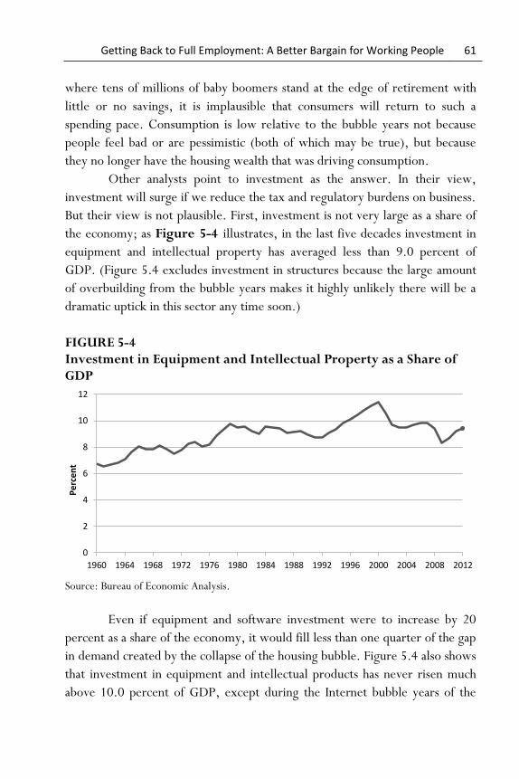
Getting Back to Full Employment: A Better Bargain for Working People 61
where tens of millions of baby boomers stand at the edge of retirement with
little or no savings, it is implausible that consumers will return to such a
spending pace. Consumption is low relative to the bubble years not because
people feel bad or are pessimistic (both of which may be true), but because
they no longer have the housing wealth that was driving consumption.
Other analysts point to investment as the answer. In their view,
investment will surge if we reduce the tax and regulatory burdens on business.
But their view is not plausible. First, investment is not very large as a share of
the economy; as Figure 5-4 illustrates, in the last five decades investment in
equipment and intellectual property has averaged less than 9.0 percent of
GDP. (Figure 5.4 excludes investment in structures because the large amount
of overbuilding from the bubble years makes it highly unlikely there will be a
dramatic uptick in this sector any time soon.)
FIGURE 5-4 Investment in Equipment and Intellectual Property as a Share of GDP
Source: Bureau of Economic Analysis.
Even if equipment and software investment were to increase by 20
percent as a share of the economy, it would fill less than one quarter of the gap
in demand created by the collapse of the housing bubble. Figure 5.4 also shows
that investment in equipment and intellectual products has never risen much
above 10.0 percent of GDP, except during the Internet bubble years of the
0
2
4
6
8
10
12
1960 1964 1968 1972 1976 1980 1984 1988 1992 1996 2000 2004 2008 2012
Pe
rce
nt

62 Dean Baker and Jared Bernstein
late 1990s. (Adding investment in structures would bring this line to 12.0
percent of GDP.) During this time, firms were able to raise billions of dollars
through issuing stock on the NASDAQ for companies that did not even have a
plan to make a profit. Yet even under those circumstances investment in
equipment and intellectual products peaked at 11.4 percent of GDP, just 2
percentage points above the 2012 level. Figure 5-5 shows the shares of all
categories of investment over the last five decades, including structures.
FIGURE 5-5 Investment as a Share of GDP
Source: Bureau of Economic Analysis.
Given the weakness of the economy and the excess capacity currently
residing in many sectors, investment now is surprisingly strong. Many firms,
most notably in the technology sector, are moving ahead with new
investments in spite of the weakness of the economy.
If we can’t expect consumption or investment to fill the hole in
demand created by the collapse of the housing bubble, we’re left with just two
0
2
4
6
8
10
12
14
16
1960 1964 1968 1972 1976 1980 1984 1988 1992 1996 2000 2004 2008 2012
Pe
rce
nt
Equipment Structures Intellectual Products

Getting Back to Full Employment: A Better Bargain for Working People 63
other candidates: net exports and government spending.36 A sound long-term
strategy would focus on increasing net exports, which means reducing the
trade deficit.
Trade and full employment
There is a great deal of confusion in policy circles, some of it
deliberate, regarding trade. When it comes to creating demand in the
economy it is net exports (exports minus imports) that matter, not just
exports. Suppose that GM decided to assemble its cars in Mexico instead of
Ohio. The company would ship all the parts that went into the car to Mexico,
and we might celebrate this surge in exports. But no additional jobs will have
been created in the United States – we had already been making the parts and
shipping them to Ohio. In terms of net exports, GM’s decision to assemble
cars in Mexico will be a loser for our economy. Exports will increase by the
value of the car parts, but imports will increase by the full value of the
assembled car, which has to be larger than just the value of its parts. Net
exports in this story fall, GDP is lower, and U.S jobs are fewer.
One can make a sophisticated argument that a higher volume of trade
alone – without a reduction in the trade deficit – can boost growth, though the
impact on employment would still be trivial. In this story, sending the car
parts for assembly in Mexico may reduce the cost of producing the car and
therefore allow it to be sold at a lower price, freeing up money for consumers
to buy other products and thereby creating jobs in other sectors of the
economy. But this is not an argument that exports directly create jobs. Rather,
it is an argument that the economy as a whole may benefit through trade by
becoming more efficient (and more efficiency lowers prices). The employment
impact, if there is one, will be on the supply side, and it will be rather limited.
As an illustration, suppose exports increased by 2 percentage points of
GDP through this sort of reshuffling of production (2 percentage points would
be a huge increase, amounting to 20 percent of current exports). If these
36 Those who have suffered through an intro economics class may recall that GDP = C + I + G +(X-M), or GDP is equal to consumption, plus investment, plus government spending, plus net exports.

64 Dean Baker and Jared Bernstein
exports allowed for an average net cost saving after transportation costs of 20
percent on the affected items, the savings would equal 0.4 percent of GDP,
the same impact as an uptick in productivity growth of 0.4 percentage points,
roughly equal to two months of productivity growth. As is the case with
productivity growth, the immediate effect is to reduce rather than increase
employment; the ultimate effect depends on how the benefits are realized
across the economy.
The immediate beneficiaries in this trade scenario would be the
companies who experience lower costs. If competition forces the companies to
pass on the lower prices to consumers, then consumers may spend on other
products and create enough jobs to offset the jobs lost to increased imports.
But if companies hold onto the gains in the form of higher profit margins, then
the result is likely to be higher unemployment, particularly if the job market is
already soft.
The jobs impact would be different in a full employment economy,
but overall not very significant. In this case, the lower price of goods
effectively raises the wages of workers by 0.4 percent, and the higher wage
will draw more people into the job market – a wage of $20.08 is a little bit
more attractive than a wage of $20. But this is a small change, and remember
that our scenario is based on a huge 20 percent boost in exports. And it is a
supply-side effect, increasing the supply of workers but not the demand for
them.37
In sum, a policy intended to substantially reduce unemployment
through trade has to be focused on reducing the trade deficit, not simply on
increasing the volume of trade. But a reduction in the trade deficit will not be
easy to accomplish in the short term. Increasing our net exports means
reducing someone else’s. In a prosperous world economy a reduction in other
countries’ net exports might be brought about without too much difficulty,
but at a time when most of our major trading partners are, like us, still feeling
the effects of the recession, it will not be easy to achieve growth at their
expense.
37 If we assume a labor supply elasticity of 0.3, then a 0.4 percent increase in the real wage would increase the number of people willing to work at the prevailing wage by 0.12 percent or roughly 180,000 workers. And this assumes a large increase in trade.

Getting Back to Full Employment: A Better Bargain for Working People 65
Still, there are areas where we can make progress. The United States
has been running large trade deficits with China and other fast-growing
developing economies, precisely the opposite of what textbook economics
predicts. We would expect rich countries like the United States to be
exporting capital and running a trade surplus with poorer countries in the
developing world because, in theory, capital can be better used and draw a
higher rate of return in the developing world, where it is scarce, than in the
United States, where it is plentiful. The developing world uses capital from
rich countries to sustain the consumption of its population while it builds up its
capital stock.
The world economy has never fit this textbook story very well, but
there were periods, such as the early and mid-1990s, when capital flowed
from rich countries to developing countries. The United States in these years
ran a trade deficit, but a relatively modest one. This situation changed with the
onset of the East Asian financial crisis of 1997, when investors pulled money
not only out of East Asia but from the developing world as a whole. The dollar
soared in value against the currencies of the countries in the region, partly
because the countries needed to export more to repay money borrowed to get
through the crisis, but partly because they wanted to accumulate massive
amounts of foreign exchange to protect themselves against future crises. The
pattern repeated throughout the developing world, as South Asian and Latin
American countries also sought to accumulate reserves to ensure that they
would not face the same sort of difficulties as the countries of East Asia did in
1997.
The cumulative effect was an explosion in the U.S. trade deficit, from
just over 1.0 percent of GDP in 1996 to more than 4.0 percent in 2000. It fell
back somewhat in the 2001 recession, but began rising again in the recovery,
eventually peaking at 6.0 percent of GDP in 2006. While the trade deficit has
declined since 2006, partly due to a decline in the value of the dollar and
partly due to the weakness of the economy slowing imports, it continues to be
a huge drain on demand. The $560 billion trade deficit (3.6 percent of GDP)
of 2012 was money that was generating demand abroad rather than in the

66 Dean Baker and Jared Bernstein
United States. In a depressed economy, that amount implies the loss of
millions of jobs.38
The key to moving from a trade deficit to a trade surplus, or at least
something closer to balanced trade, is to reduce the value of the dollar against
other currencies. If the dollar falls in value, then imports become relatively
more expensive for people in the United States, leading us to buy fewer
imports and more domestically produced goods and services. At the same
time, our exports become cheaper, and people in other countries buy more of
our products. Importing less and exporting more generates additional demand
in the U.S. economy; actually having balanced trade (there is no magic to
balanced trade, just like there is no magic to a balanced budget) would take us
far toward full employment. Moreover, we can expect a multiplier effect on
GDP as a result of the “re-spending” by people employed (largely in
manufacturing) as a result of the elimination of the trade deficit. People who
are newly employed in export industries, or in industries producing goods that
replace imports, will spend much of their pay, and this will lead to additional
consumption demand. If this re-spending effect is half the size of the change in
the trade balance (this is in keeping with most estimates of the size of the
multiplier), then the move to balanced trade would increase GDP by $840
billion, or close to 5.4 percent. A proportionate increase in employment
would imply an additional 7.5 million jobs in the economy. Put another way,
if Okun’s law is correct – that a 2.0 percentage-point rise in GDP is associated
with 1.0 percentage-point drop in the unemployment rate – then a 5.4
percentage-point rise in GDP would be sufficient to lower the unemployment
rate by 2.7 percentage points, which would have gotten us under 5.0 percent
in the summer of 2013.
While balanced trade might be too ambitious a goal given the
persistence of trade deficits over the past 15 years, the rise in the number of
jobs associated with moving to balanced trade would get the U.S. economy
38 There are many excellent papers that document the impact of this rise in imports on jobs and wages. For example, Autor, Dorn, and Hansen (2011) show a strong link in local labor markets between imports from China and manufacturing jobs and wages. Krugman (2008) shows that the rapid growth in imports from China over the prior decade was large enough to have a substantial impact on the U.S. labor market.

Getting Back to Full Employment: A Better Bargain for Working People 67
close to full employment. A lower-valued dollar rests at the center of this
effort. Trade agreements, insofar as they lower barriers to trade between the
United States and one or more trading partners, may boost trade, and they
may produce gains in efficiency, but there is no theoretical reason or empirical
evidence to suggest that they will help to lower the trade deficit. Some aspects
of recent and pending trade deals may actually impede growth. A central
feature of nearly all trade deals is the strengthening of patent and copyright
protection. These rules have the effect of raising the prices of the protected
products, like drugs or computer software, and the higher prices pull money
out of the economy and cause it to be less efficient, at least in the short term.
While the net impact on jobs may be small, it is nevertheless negative.
Another approach that has been suggested for reducing our trade
deficit is to make U.S. producers more competitive by improving the
education of workers and upgrading our infrastructure. Some important points
about this agenda need to be taken into account.
First, reducing the trade deficit by better educating our workforce and
improving our infrastructure is at best a long-term strategy. In the next five or
even 10 years, only a small fraction of our workforce will benefit from
whatever educational upgrading we hope to bring about. Moreover, we have
little empirical support for such a claim. The United States began running
persistent trade deficits starting in the latter 1970s, but since then the share of
workers with college degrees has about doubled, from around 15 percent to
30 percent. The same hurdles apply to infrastructure. Small projects can be
accomplished quickly, but almost by definition these will have a limited impact
on the cost of goods production. Bigger infrastructure projects, like high-speed
rail, will take years and possibly decades to put into place.
The second qualification about educational and infrastructure
improvements is that there are no guarantees with these investments. Based on
past experience we can expect that on average public investment will add at
least as much to productivity as private investment, but this doesn’t mean that
some investments will not turn out poorly.39 This is crucial to keep in mind,
39 For discussions of the productivity of public investment, see Aschauer (1989); Munnell (1990); Heintz et al. (2009); Heintz (2010); and Holtz-Eakin (1992).

68 Dean Baker and Jared Bernstein
since if the public is not prepared to see some initiatives fail, we can expect to
see a backlash against a public investment agenda.
Finally, even in the best case the benefits of an aggressive public
investment agenda will be limited. For example, a $3 trillion increase in public
investment over the next decade (an unlikely possibility in this political
climate) that yielded an annual return of 15 percent (a high rate) would boost
GDP 10 years from now by $450 billion, or a bit less than 2.5 percent. This
would mean that the same number of workers could produce 2.5 percent
more output. If wages did not rise in step with this increase in productivity
then our goods would sell for roughly 2.5 percent less relative to those of our
competitors as a result of this massive investment. This is far from trivial, but
it does not represent the sort of gain in efficiency that could substantially
reduce a trade deficit of 3-4 percent of GDP.
Instead of negotiating unpopular trade agreements, educating a
workforce, much of which is already academically well-equipped, or waiting
for public investment to yield its dividends, we can confront the trade deficit
directly and immediately by reducing the value of the dollar. A drop in the
dollar by 10 percent against other currencies is equivalent to a 10 percent
increase in the productivity of the U.S. economy, assuming no offsetting
increase in wages. This swamps any plausible increase in productivity even
with a very effective program of improved education and infrastructure.
The drop in the dollar from its peak in the last decade has brought the
non-oil trade deficit almost down to where it was before the run-up in the
dollar in the late 1990s.40 In 1996, before the East Asian financial crisis sent the
dollar soaring, the non-oil deficit was less than 0.3 percent of GDP. It peaked
at 3.7 percent of GDP in 2004, three years after the peak of the dollar, and
40 It is often claimed that a lower dollar will be inflationary. While a lower-valued dollar will have some inflationary impact, the size is likely to be small. The dollar has lost more than 20 percent of its value against a trade-weighted basket of currencies since its peak in 2002, yet we have been more concerned about deflation over this period than inflation. The arithmetic works like this. Our imports are roughly 16 percent of GDP. An increase in the price of all imports of 10 percent (a very large increase) would effectively raise prices in the United States by 1.6 percentage points. If this took place over three to four years, it would effectively add 0.4 to 0.5 percentage points to the annual inflation rate each year. This rise could be easily absorbed in an economy with productivity growth averaging close to 2.5 percent (at least prior to the downturn.)
Getting Back to Full Employment: A Better Bargain for Working People 69
had fallen back to 0.8 percent of GDP in 2012, following the dollar back to its
former level.
But counting oil, for which the United States paid far more in 2012
than it did in 1997, the trade deficit is still large. In textbook economics the
higher price of oil imports should lead to a further decline in the value of the
dollar, as increased exports and reduced imports of non-oil products offset the
impact of higher oil prices. (The logic is that paying more money for imported
oil increases the supply of dollars and thereby reduces the price of the dollar
relative to other currencies.) Recent experience suggests that the decline in
the value of the dollar has had pretty much the predicted effect on the trade
balance, but it is necessary for the dollar to fall further to offset the impact of
higher world oil prices.
The value of the dollar is not the only thing that determines the trade
balance. A second factor is relative growth rates. If the U.S. economy grows
rapidly and the economies of our major trading partners grow slowly, then our
trade deficit will tend to rise (vice-versa if the opposite is the case), because a
country with a booming economy will generally have more rapid import
growth, worsening its trade deficit. A third factor is history. If the United
States starts buying more steel from abroad when the dollar is overvalued, the
steel industry may not come back when the dollar later falls. Once production
is shipped overseas, domestic factories close and workers go elsewhere.
Bringing back plants and workers is a high hurdle.
However, the idea that a lower dollar will improve the trade balance
is well supported by the evidence. If the dollar were to decline further we can
be fairly certain that the trade deficit will move closer to balance, helping to
fill a large part of the hole in demand created by the collapse of the housing
bubble.
Contrary to what we often hear, the United States is not helpless in
determining the value of the dollar. In principle all the steps that other
countries have taken to keep down the value of their currencies, such as
buying up large amounts of dollars, the United States could take as well. Some

70 Dean Baker and Jared Bernstein
currencies, like the Chinese yuan, are not freely traded, but there are
measures that could be taken even in these cases.41
Negotiation will be key. If the United States is going to persuade
countries to raise their currencies relative to the dollar, then it will have to be
prepared to make offsetting concessions, at least with more powerful countries
like China. These could include, for example, placing a lower priority on
getting China to respect U.S. patents and copyrights, or providing better
access to China’s domestic market to U.S. financial firms or other sectors.
Surely there are some concessions that the United States could make to China
that would persuade it to raise the value of its currency. That negotiations to
date have not led China to do so is likely due to the fact that the United States
has not placed a lower-valued dollar at the top of its agenda.
The obstacle to a lower-valued dollar is neither the architecture of the
international financial system nor the intransigence of our trading partners.
Rather, it is a lack of political will on the part of U.S. administrations. A
lower-valued dollar is far from the only concern raised in negotiations, but it is
not clear that it is even a high priority. Of course, powerful interests benefit
from an overvalued dollar. For example, Walmart and other large retailers
have established low-cost supply chains in China and other developing
countries, and these are an important advantage these companies hold over
smaller competitors. They will lose this advantage if the dollar declines
sharply. Similarly, most large U.S. manufacturing corporations have set up
operations in the developing world, where lower labor costs allow them to
undercut domestically based manufacturers. These companies are also not
41 For example, Joe Gagnon has suggested that the government could impose high taxes on the earnings of the dollar assets of foreign central banks (Gagnon and Hufbauer 2011). It is also possible to try to push up the value of other currencies against the dollar by buying up futures on those currencies. The idea would be that a sharp rise in the value of the futures would lead to a rise in the current market price as traders tried to acquire the currency now in order to take advantage of the higher future price. Finally, the government could encourage holders of a currency to violate their government’s laws against trading simply by offering them a good price. If the official price of the Chinese yuan is 20 cents, the U.S. government could offer to buy yuan for 25 cents; the opportunity for substantial guaranteed gains is likely to lead many holders of yuan to sell them to the U.S. Treasury. If this were to happen on a large enough scale, then the effective exchange rate for purposes of trade would be the rate set by the Treasury.

Getting Back to Full Employment: A Better Bargain for Working People 71
anxious to see the dollar fall and thereby reduce their competitive advantage.
It is likely that these domestic interests are a bigger obstacle to achieving a
lower-valued dollar than foreign governments are.
For these reasons, there is hardly unanimity among constituencies in
the United States for a lower-valued dollar, even if it will get us to full
employment without large budget deficits. The issue has, however, gotten
some attention in Congress. Representative Sander Levin and Senator Sherrod
Brown have proposed legislation that would retaliate against China for its
currency policy. This bill has received considerable support in both houses,
but most observers consider the support to be primarily for show. It is unlikely
that the bill will ever pass Congress, and President Obama would almost
certainly veto it if did.
Conclusion
The large trade deficit that the United States has been running over
the last 15 years has created a substantial gap in demand. In the late 1990s the
gap was filled by demand generated by the stock bubble, and in the last decade
the housing bubble stood in. But we should not look to asset bubbles to sustain
high levels of unemployment. Instead, we should have a policy focused on
getting the trade deficit closer to balance.
While there are many policies, such as improving education and
infrastructure, that will increase the economy’s productivity, even in a best-
case scenario these strategies can have only a marginal impact on the trade
balance in the near term. The trade deficit was relatively modest until the late
1990s, when the East Asian financial crisis led to a run-up in the value of the
dollar. While the dollar has since reversed much of this gain, it needs to fall
still further. Lowering the value of the dollar is not a difficult task
economically; the problem is political. Powerful domestic interest groups
benefit from an overvalued dollar, and getting it down to a level consistent
with more balanced trade will mean overcoming the opposition of these
special interests.

72 Dean Baker and Jared Bernstein
Chapter 6
Policies for Full Employment II: Public Investment, Public Jobs, and Work Sharing
The collapse of the housing bubble in 2007 left the economy with a
shortfall in annual demand of more than $1 trillion. Since then, Washington’s
most significant responses have been the American Recovery and
Reinvestment Act of 2009 and efforts by the Federal Reserve to keep interest
rates low and supply liquidity. Though these have been positive steps, they
clearly haven’t gone far enough to lastingly offset the magnitude of the
downturn. In Chapter 4 we argued that the Fed should go further, by raising
(or eliminating) its inflation target, and in Chapter 5 we urged the
administration to take steps to lower the value of the dollar and thereby the
trade deficit. Those are two prongs, and this chapter offers three more.
The first is public investment. Downturns are characterized by a drop-
off in demand that the private sector is unable to fill. The government, with its
capacity to borrow on favorable terms, can afford to spend when everyone else
is hunkered down. Some forms of spending are better than others in terms of
reinvigorating demand, and one of the best forms is public infrastructure
investment, which can employ hundreds of thousands of workers in projects
that yield long-term, continuing returns on the dollar.
The second policy idea is to launch a system of publicly funded jobs
that can ramp up and down, expand and contract, as needed, in tandem with
the business cycle. Under such a system the federal government, working
Getting Back to Full Employment: A Better Bargain for Working People 73
through local intermediaries, would supply funds to subsidize hiring in the
private sector as well as in important community services like education, child
care, and recreation.
Finally, we can take steps to ameliorate the disemployment effects of a
downturn by sharing work, and we can counteract productivity-driven drops
in demand for labor by restructuring work. Under work sharing, employers
would address drops in demand by reducing hours across their workforces
instead by laying off an unfortunate few; the government funds that would
otherwise have gone to unemployment benefits could be used to partially
make up everyone’s lowered wages that result from working shorter hours.
On the other side of the coin, what happens when gains in worker productivity
lessens the demand for workers? If the gains are shared with workers (a big
assumption, but once typically the case), then either fewer will work, but for
more money, or as many will work, but for fewer hours. The former rewards
some but risks unemployment; the latter spreads the benefits, maintains
workers’ attachment to the labor market, and gives the gift of time – for
family life, education, child care, or just plain leisure. Guaranteed vacation
days, sick time, and family leave, taken for granted among our international
competitors but virtually nonexistent in the United States, can help to
restructure work so that gains from productivity to broader gains than simply
than a higher GDP.
The budget deficit, low-cost borrowing, and full employment
If a nation that is running a large trade deficit wants to achieve full
employment, it will probably have to run a budget deficit. The existence of a
trade deficit means that there is a gap in demand, created in and unmet by the
private sector. To restore demand and create jobs, the public sector has to fill
the gap, and this means running budget deficits. When a trade deficit is
compounded by a contraction in private demand during a downturn, a budget
deficit is an essential part of the cure.
Most people are adverse to budget deficits not only because politicians
constantly harp on them but also because we know in our personal lives that
continually borrowing money leads to trouble. But there are a couple of
important points that we need to recognize about deficits, especially in the

74 Dean Baker and Jared Bernstein
context of a shortfall in private-sector demand like the one our economy now
faces.
First, government is fundamentally different from an individual
person. None of us can expect to continually run up ever more debt through
our lifetimes, because at some point creditors, knowing that they will never be
paid back since we can’t work forever, will stop lending us money. This is not
an issue for governments since, barring an extraordinary disaster, we expect
them to survive indefinitely. (Of course even with individuals we all recognize
that some borrowing, like student loans or a home mortgage, make good
sense.) It is the same with corporations – large profitable companies like
AT&T and General Electric can and do, as long as their borrowing costs are
reasonable compared to profits, borrow forever. In fact, borrowing may be
the best route for them to reach their productive potential and generate high
returns to shareholders.
But governments have a duty that corporations don’t. While
corporations are responsible only for returns to their stakeholders,
governments are responsible for the health of the economy, which means that
they have the responsibility to sustain demand during a downturn by taking on
more debt. In this context borrowing is the only responsible path for policy.
The alternative is to allow for the economy to operate below its capacity
indefinitely and keep millions of workers needlessly unemployed.
This would be a foolish and wasteful policy even if the costs of
recession were equally shared, but they’re not. They fall disproportionately on
the most economically vulnerable, and so living with depressed labor demand
distributes income upward from the bottom and the middle of the income
distribution to the very top. This is not just theory: After four years of weak
recovery in the labor market – and declining deficits – the stock market is up
66 percent and GDP is up 9 percent, but weekly paychecks are up just 2
percent and median household income is down 4 percent.42
42 All values adjusted for inflation. The stock market figure is from the S&P 500 index, real GDP is from the Bureau of Economic Analysis, weekly earnings of nonmanagerial or production workers are from the Bureau of Labor Statistics, and median household income is from Sentier Research.

Getting Back to Full Employment: A Better Bargain for Working People 75
The second point that we need to consider about indebtedness is that
the burden on the government is best measured by the interest paid, not the
total value of the debt. The latter changes in response to changes in interest
rates. A 30-year bond that pays 3 percent interest will sell for its face value if
the current interest rate on 30-year bonds is 3 percent. But if the interest rate
on newly issued 30-year bonds is 6.0 percent, then anyone looking to sell the
older bonds will have to offer them at a discount.43
Focusing on the interest burden rather than the value of the
outstanding debt yields a very different picture of the country’s indebtedness
than we might have expected given the drumbeat on the deficit. Instead of
rising to extraordinarily high levels, our interest burden sits near postwar
lows, as shown in Figure 6-1, even as the debt burden has risen sharply.44 The
bottom line is that the government is nowhere near the limit of its ability to
take on additional debt. Even if we go out 10 years and assume no further
deficit reduction, the interest burden that the government would face in 2023
is projected to be only as large as the burden faced in the early 1990s; while
not a trivial amount, it did not prevent the 1990s from being the second-
43 The relationship between interest rates and bond prices can be illustrated with a simple bond calculator such as the one at Smart Money (http://www.smartmoney.com/calculator/bonds/bonds-calculator--bonds--bond-funds-1309988621833/). Since the market value of the bonds issued during the period of low interest rates will fall when interest rates rise, the market value of that portion of the government’s debt will fall, even though the interest burden will be unchanged. If it wanted the government could buy back those bonds, reducing the value of its debt. There would be no real reason to carry through this sort of bond flipping, but if we felt that the value of our debt was an important factor affecting the health of the economy, then buying back bonds at sharp discounts would be a nearly costless way to shave hundreds of billions of dollars off of the national debt.
44 The interest burden would be even lower than implied by Figure 6-1 if we factored in the interest payments refunded by the Fed. The Federal Reserve Board held more than $3 trillion in government bonds and other assets at the end of 2012. The earnings from these assets are paid back to the Treasury at the end of the year; in 2012 the Fed refunded more than $80 billion to the Treasury. If this money is subtracted from interest, the burden in 2012 was less than 0.6 percent of GDP, lower than at any point in the post-World War II era. While the Congressional Budget Office projects that the Fed will sell off most of its assets in the next few years, it could in principle hold the assets indefinitely. While doing so would raise issues for the conduct of monetary policy, it could substantially reduce the interest burden of the debt in the decades ahead.

76 Dean Baker and Jared Bernstein
strongest decade of growth in the post-World War II era, after the 1960s.
Clearly, we are not facing unmanageable debt anytime in the near future.
FIGURE 6-1 Net Interest as a Percent of GDP
Source: Congressional Budget Office.
It is of course possible for a government to face runaway debt that is
not tenable in the long run. For example, long-term projections for the U.S.
budget show ever-expanding deficits driven primarily by an explosion in health
care costs. If per-person health care costs outpace the growth of GDP going
forward, government health care programs like Medicare and Medicaid will
eventually impose an unbearable burden on the Treasury. In the absence of tax
increases or cuts in health benefits, these deficits would almost certainly lead
to sky-high interest rates and/or inflation.
But there are two points that are important to consider about these
projections. First, the assumption behind them is that health care costs outpace
the rate of growth of the economy for long periods. Yet in recent years health
care costs have slowed considerably, and at least for now, the gap between
economic growth and health care cost growth is much smaller. In any case,
rising health care costs are not a problem of extravagant government spending.
The United States spends more than twice as much per person on health care
than do other wealthy countries, with too little to show for it in the way of
outcomes relative to these other advanced economies. Out-of-control health
care spending is a burden on the economy whether or not the government is
picking up the tab.
0.0
0.5
1.0
1.5
2.0
2.5
3.0
3.5
19
73
19
75
19
77
19
79
19
81
19
83
19
85
19
87
19
89
19
91
19
93
19
95
19
97
19
99
20
01
20
03
20
05
20
07
20
09
20
11

Getting Back to Full Employment: A Better Bargain for Working People 77
In other words, the long-term projection of spiraling spending is a
health care cost problem, not a budget problem. If the recent slowdown in
cost growth continues, and the cost control measures in the Affordable Care
Act prove effective, then our longer-term budget problems are likely to be
manageable. If health care costs again start to grow rapidly, then we will have
to revisit the issue and figure out a more effective way to control costs.
The second point about long-term projections is that they are long-
term projections, and as such they must be kept in perspective. We have an
immediate problem --millions cannot find any or enough work—and we can
address this problem with measures that will lead to higher deficits. If in 10-15
years these large deficits are a problem, we can deal with them.
History is a guide here. The first President Bush secured a substantial
deficit reduction agreement in 1990, and President Clinton did so in 1993.
Under President Obama, spending cuts and tax increases have lowered
projected 10-year deficits by almost $3 trillion, and the deficit-to-GDP ratio is
down from 10 percent in 2009 to 4 percent in 2013 (Kogan and Van de Water
2013). If we’ve done it before we can certainly do it again, though the current
dysfunctional Congress does give sensible people cause for worry.
One of the most peculiar arguments about deficits is that we must save
our children from the phantom menace of future debt tomorrow by severely
underinvesting in them today. We must defund Head Start, public schools,
universities, libraries – not to mention our own employment opportunities.
This absurdity is accepted wisdom in today’s fiscal debates, even though the
extraordinarily low interest rates at which the government can borrow money
would be taken as a signal by any private investor that now is a good time to
borrow. If government were run like a business, it would be taking advantage
of low interest rates to finance a wide variety of public investments. Franklin
Roosevelt did that during the New Deal, undertaking infrastructure projects
that still support the economy today.
What kinds of work does the federal government need to get done
today? The list of projects that could be usefully undertaken is lengthy. Some,
such as road and bridge repair, are simple and obvious. The Recovery Act
funded a number of improvements in road and bridge infrastructure. A more
ambitious but productive undertaking would be high-speed rail. The United

78 Dean Baker and Jared Bernstein
States lags badly behind other wealthy countries in its regional and long-range
rail system. Japan and Western Europe have had trains that can travel more
than 170 miles per hour for four decades. While trains will likely never be
competitive with airlines for coast-to-coast travel, they can be competitive for
trips of 300-700 miles, which comprise a large portion of trips in the United
States.
A major area for investment is our building stock – homes, businesses,
and government buildings – which is far less energy efficient than the building
stock in Europe or Japan. In many cases, modest spending on insulation and
other improvements will produce sharp reductions in energy use. Some
funding in the ARRA was devoted to this purpose, but there are undoubtedly
millions of structures that would benefit from energy-efficiency retrofits.
Infrastructure also includes communications. Historically, the United
States has been at the forefront in communications, building out its phone
system and then its Internet system, but now we lag many other countries in
extending access to high-speed Internet. Building up broadband networks so
that everyone has low-cost access to high-speed connections should be a
priority not only for economic but also for equitable reasons. Children in
homes with slow or no Internet access will be at a serious disadvantage against
their better-connected peers. We structured telephone regulation with
universal access as an explicit goal, and we should take the same approach with
broadband.
The country can also take advantage of low-cost borrowing to build up
its human capital. A period in which the private sector is not creating many
jobs is a great time for people to gain additional skills. This is an argument for
a more-generous-than-normal student loan or grant policy to encourage
people to go to school.
A large-scale youth employment program could give disadvantaged
young people valuable work experience. The unemployment rate for teens
overall was 24.0 percent in 2012; for African American teens it was 38.2
percent, and in many depressed urban areas it was likely over 50 percent. The
private sector clearly is not offering enough jobs for teens, and unemployment
can hardly be seen as an acceptable start to a young person’s work career. A
youth jobs program would require relatively little money or advanced planning

Getting Back to Full Employment: A Better Bargain for Working People 79
to hire young people to clean up streets and parks, board up abandoned
buildings, and perform other relatively simple tasks that could improve the
quality of life in urban areas. While these jobs might be derided as “make
work,” it is not clear what the downside is. The vast majority of these workers
would not have otherwise been employed, and it seems like common sense to
offer young people, who otherwise would have almost no job prospects, the
opportunity to earn a modest wage improving conditions in their
neighborhoods.
The need for a national jobs program
We widely accept the role of the Federal Reserve as the “lender of last
resort” during financial panics, when credit is in short supply. The failure of
the market to hire capable and willing workers is no less serious than the
failure of banks to lend. If our central bank, a government institution, can be a
lender of last resort, then the federal government can also be the employer of
last resort. This conclusion is particularly germane as we think about how our
safety-net programs have evolved to become increasingly dependent on work.
If our policy is to make employment a requirement for receiving public
assistance, then we have an obligation to offer a job if the marketplace isn’t
doing so.
For example, consider a national program to modernize the nation’s
public schools. The average public school building is 40 years old, and many
lack adequate insulation, windows, and heating and cooling systems, even
though research shows that upgrading school environments is associated with
better student outcomes. Legislation to fund the upgrading of schools has been
introduced in both chambers of Congress, but it languishes there.
The nation needs a flexible program of publicly funded jobs that can
ramp up and down as needed. A model for such a program is the ARRA-
funded Temporary Assistance to Needy Families (TANF) Emergency Fund.
During 2009 and 2010, before its funding expired, the program spent $1.3
billion to place about 260,000 low-income parents into jobs, for which it
typically paid 80% of the wages (the program also included a summer jobs
component of the type discussed in the previous section). Many were skeptical
80 Dean Baker and Jared Bernstein
that such a program could be up and running quickly and efficiently, but in less
than six months Illinois alone had placed 30,000 low-income workers in
subsidized jobs.
How do such subsidized jobs programs work? Typically, the federal
government supplies funds to a local intermediary, including local
governments, nongovernmental organizations, workforce investment boards,
and low-wage worker advocacy groups, to work with private and public
employers to create jobs. The subsidized jobs through the TANF fund were
mostly in the private sector, in administration, sales, customer service,
construction, food service, and health care (Pavetti et al. 2011). Researchers
have suggested that employment in these programs can provide important
community services, like the maintenance of schools, libraries, and community
centers; cleanup of abandoned and vacant properties; and support to the staffs
of overburdened programs like Head Start, child care, and school-based
literacy initiatives (Johnson et al. 2010).
The program demonstrated that there’s a lot of work to be done, and
a lot of unemployed and underemployed people to do it. Yet political barriers
exist to ideas like these, for a variety of reasons. The TANF jobs program was
allowed to end in 2010, well before labor market conditions warranted its
demise. Cliff Johnson, an analyst who has extensively studied the history of
public jobs programs, summarizes the problem:
“In many respects, the reluctance of key policymakers to launch a new
[public jobs] program this past year was rooted in a fundamental misreading of
past research. Past experience provides ample evidence that public job
creation can be undertaken quickly and effectively, with acceptable costs,
manageable levels of substitution or displacement, and clear benefits to
participants and their communities.” (Johnson et al. 2010)
The displacement point is important, because incentives exist in these
programs for an employer to replace unsubsidized workers with subsidized
ones, resulting in no net impact on employment and a wasteful transfer from
taxpayers to employers. Thus, oversight should be built into the programs,
penalties levied against employers found violating the displacement rules,
hotlines established for laid-off employees who suspect they’ve been displaced,
and protections offered to those on leave or on strike.

Getting Back to Full Employment: A Better Bargain for Working People 81
Programs like the TANF Emergency Fund have shown that they can
ramp up quickly in recessions, and that employers will respond to the offer of
subsidized employment. This function could be implemented even more
efficiently if we planned for the bad times during the good times. Building up
an infrastructure of intermediaries to help match subsidized workers with jobs,
without displacement, would facilitate a smoother, quicker implementation
next time.
But such programs are likely to be needed in expansions as well as
downturns. In the current expansion, not only has job growth been weak, but
the number of long-term unemployed (jobless for at least six months) has been
historically high. Research has shown that, even when their skills remain
relevant, the long-term unemployed have a harder time getting re-employed
based simply on the stigma of joblessness attached to them. Thus, a transitional
jobs program, which could offer extra services to hard-to-employ populations
or simply provide a temporary public or subsidized private job to a long-term
unemployed person, would be a useful component of a strategy of publicly
funded jobs. For the long-term unemployed, it will be easier to find a
permanent job if they’ve already got a temporary one.
Work sharing and restructuring work
The last two sections focused on increasing employment by raising
output: If we produce more, we will need more workers. But there is another
way to employ more workers, and that is by dividing the existing work among
more of us by having the average worker put in fewer hours.
The math works like this. If we require 200 billion hours of work at
the current level of output, and the average worker puts in 2,000 hours, we
need to employ 100 million workers. But if the average worker put in 10
percent fewer hours (1,800), then we would need to employ 111 million
workers to get 200 billion hours of work. By reducing the average number of
hours per worker, we hire more workers at the same level of output.
In the real world things will never be as simple as this arithmetic
implies, but the basic principle, that we will have more workers employed if
the typical worker puts in fewer hours, holds true. In fact, several countries,

82 Dean Baker and Jared Bernstein
most notably Germany, have successfully implemented policies to shorten
average work hours as a way to keep workers employed through the
downturn. In the case of Germany, its unemployment rate has actually fallen
by more than 2.0 percentage points from its pre-crisis level, in spite of the fact
that its economic growth has been no better than that of the United States.45
The difference is even more striking on the employment side of the equation.
Germany’s employment-to-population ratio for workers age 16-64 rose by 3.8
percentage points from 2007 to 2012. Over the same years the ratio fell by
4.7 percentage points in the United States.
A big part of Germany’s success has been its policy of Kurzarbeit, or
short-work, under which the government makes up a portion of the wages that
workers lose as a result of the shortening of the workweek. The logic is
straightforward. Under a traditional system of unemployment insurance the
government makes up a fraction (say 50 percent) of the wages of workers who
are completely unemployed. Under Kurzarbeit the government makes up the
same fraction of the pay of workers who are partially unemployed.
In the case where the government covered 50 percent of wages, a
cutback in hours of 20 percent would mean that a worker would end up
working 80 percent as many hours as he or she had previously (possibly in a
four-day workweek) for 90 percent as much pay. While the loss of pay would
likely still involve some hardship for workers, it is certainly less than if they
were unemployed. In addition, because workers stay on the job, they do not
have the same risk of falling into a period of long-term unemployment and
losing their attachment to the workforce. Instead, they will be having their
skills continually upgraded, as will their colleagues at work, as companies
adjust their production in response to changes in demand and technology.
This system has worked well in Germany in part because it has a long
tradition of labor–management cooperation. About 20 percent of Germany’s
workforce is unionized, but collective bargaining covers a much larger share,
about 60 percent (in the United States only about 11 percent of the workforce
45 The underlying size of Germany’s labor force is growing more slowly than the United States’, so the country would need less rapid growth to keep its unemployment rate from rising. However, the difference in demographics would explain only a small part of the difference in labor market outcomes since the onset of the recession.

Getting Back to Full Employment: A Better Bargain for Working People 83
are union members and 12.5 percent are covered by agreements).46 Under
German law, all large companies have workers’ councils that provide a formal
opportunity for worker input regardless of whether or not the workers are
unionized. In this environment it is easier to arrange for reductions in hours,
since there is more of an atmosphere of trust between workers and
management. The United States does not have the same tradition, and workers
will inevitably be more suspicious of management efforts to adjust work hours
to deal with a falloff in demand.
Nonetheless, there have been some efforts at work sharing in the
United States. Twenty-five states, including California and New York, have
incorporated short-work programs into their state unemployment insurance
systems. Most of the programs were implemented in the late 1970s or early
1980s and have not been updated. They are often overly bureaucratic, and few
employers even know about their existence. For these and other reasons, take-
up rates have been low.
The Obama administration has made a modest effort to promote short
work as an alternative to layoffs. The law extending the payroll tax cut into
2012 also called for the federal government to pick up the full cost of these
short-work programs in the states that already had them in place and to
provide money for other states to establish the programs. In principle, the law
gives states substantial incentive to promote their short-work programs, since
it means they can save money that they otherwise would have spent on
unemployment insurance. But the response has been limited, and short-work
programs continue to be little known, even in the states that offer them, and
governments have done little to publicize their existence.
Remember that these work-sharing programs are intended to be an
alternative to layoffs. Under the system of unemployment insurance, if a
company were to lay off 20 percent of its workers, the government would
effectively be paying these workers half of their pay to be unemployed. There
is no reason as a matter of public policy for the government to encourage firms
46 See Figure 1 in Nicola Düll, “Collective Wage Agreement and Minimum Wage in Germany,” European Employment Observatory, available at http://www.eu-employment-observatory.net/resources/reports/1-Germany-NationalAdHocResponseMinimumWage-final.pdf.
84 Dean Baker and Jared Bernstein
to lay people off rather than reduce work hours across the firm. Work sharing
is a way of leveling the playing field, with the government making up half of
the lost pay for workers who are forced to work fewer hours.
As noted above, there are good reasons why shorter hours rather than
layoffs would be the preferred policy from a social standpoint: workers
maintain their attachment to the labor force, continue to use and sharpen their
skills, and avoid the trauma of job loss and perhaps long-term unemployment.
Short work is also likely to help support the labor market more generally. The
unemployed would be desperate for work in a way that people working short
hours would not be, and there is likely to be more downward pressure on
wages when 8 percent of the workforce is unemployed than when 20 percent
of the workforce is working shorter hours.
In Germany the short-work policy has near universal support. It was
originally implemented by a Social Democratic minister in a left-right unity
government, but it has been enthusiastically embraced by the Christian
Democrats in the years that they have held power on their own. While unions
have mostly been pleased with keeping their members employed, businesses
also value the flexibility that the policy provides. By retaining skilled workers
on the payroll, work sharing leaves firms well-situated to deal with any upturn
in demand. Rather than finding and training new workers, companies can
simply increase hours for their existing workforce.
On the other hand, work-sharing programs have and will continue to
be used less to promote full employment than to accommodate its absence.
That is, when output gaps arise because the economy is operating below full
potential, work sharing spreads the pain of inadequate demand. Instead of the
unemployed bearing the entire burden of labor slack, the labor market shares
it more broadly, meaning that we trade off less unemployment for more
involuntary underemployment. The optimal public policy is still full
employment, which provides workers the hours of work they seek.
The use of short work to sustain employment raises a more general
issue of how we think about work time and full employment. The business
pages are full of stories warning that robots and other new technologies will
diminish the need for human labor in the years ahead, and the result will be
massive unemployment as labor-replacing technology eliminates work for
Getting Back to Full Employment: A Better Bargain for Working People 85
large numbers of people.47 History is littered with such predictions, and there
are many aspects to today’s version that don’t hold up to scrutiny. For
example, they imply an acceleration of productivity growth in recent years,
but that has not occurred. Still, recent advances in computerization, artificial
intelligence, and robotics may yet show up in the productivity accounts and in
higher unemployment. But this raises a fundamental question: Why should a
reduced need for labor be a cause for concern?
Let us be careful to distinguish between too little demand for labor – a
problem that motivates this book – and reduced need for labor. Imagine that
the economy at full capacity would create $20 trillion in output. In the case of
insufficient demand, output is notably below $20 trillion, meaning output,
jobs, and incomes are left on the table because of a shortfall in demand. In the
reduced need case, however, technology enables us to generate the $20
trillion with less work.
In this scenario, the reduced need for labor allows us all to be richer,
as it in fact did in the three decades immediately following World War II. In
those years productivity increased at almost a 3.0 percent annual rate, and the
gains from this growth were broadly shared, with workers up and down the
income ladder seeing rapid rises in living standards.
In the years after 1980 the gains from productivity growth have gone
increasingly to those at the top of the earnings scale. There are a variety of
reasons for this, with less-than-full employment being one of them.
Historically, one way in which workers have taken the benefits of productivity
growth has been through shorter workweeks and/or work years. The eight-
hour day/40-hour workweek was one of the major demands of the labor
movement in the United States dating from the late 19th century. It was
eventually put into law with the Fair Labor Standards Act in 1938.
Workers have also sought to reduce the duration of the work year
with paid holidays, paid vacations, sick days, and family leave. In the United
47 Remarkably, many of the same news outlets, and sometimes even the same reporters, also have reported stories about how the rising ratio of retirees to workers threatens to impoverish the current generation of young people. Somehow we are supposed to believe in a future with both an enormous glut of workers due to the progress of technology and a dire shortage of workers due to changing demographics. This future does indeed look bleak.

86 Dean Baker and Jared Bernstein
States, these reductions in the duration of the work year have largely been at
the level of the individual employer or negotiated as part of a union contract.
There are no national guarantees of paid time off.48 As a result, the length of
the average work year for full-time workers has remained about the same for
the last three decades.
The stagnation in the length of the workweek/work year has led some
people to view the 40-hour workweek and skimpy vacation time as somehow
natural. It is not – this just happened to be the point where we largely stopped
our reduction in work hours. It makes as much sense to view the current
workweek or work year as natural as it does to view a particular median
hourly wage as natural, and the latter has also changed little over the last three
decades.
In contrast to the United States, all countries in Western Europe
mandate considerable amounts of paid leave (Figure 6-2). For example, as a
condition of joining the European Union a country must guarantee its workers
at least four weeks of paid vacation each year. The United States stands out as
the only country that does not guarantee its workers some amount of paid
vacation or holidays.
In addition to paid vacation, all other wealthy countries guarantee
their workers some amount of paid sick time and paid family leave (Ray et al.
2008; Heymann et al. 2009). Also, in many European countries, most notably
France, the standard workweek is considerably less than 40 hours.
The net effect of these various forms of paid leave and reductions in the length of the standard workweek has been a sharp reduction in the length of the average work year in these countries. While the average work year in the United States is still almost 1,800 hours, it is just over 1,700 in Canada and 1,625 in the United Kingdom. The average work year is less than 1,500 hours in France, and just over 1,400 hours in Germany (Figure 6-3).
48 The Family and Medical Leave Act, passed in 1993, guaranteed workers at firms employing more than 50 workers at least three months of unpaid leave to attend to newborn children or sick family members and to meet other medical needs. California and New Jersey require most employers to provide up to six weeks of paid family leave to most workers to care for young children or sick family members. Several cities have laws that provide some guarantee of paid time off, but the vast majority of workers in the country have no government guarantee of paid time off.

Getting Back to Full Employment: A Better Bargain for Working People 87
FIGURE 6-2 Paid Vacation Days and Paid Holidays In OECD Countries (including United States)
Source: Ray, Sanes, and Schmitt 2013.
FIGURE 6-3 Average Annual Hours Worked OECD
Source: OECD 2011.
30 28
25 25 25 25 22 22 22
20 20 20 20 20 20 20 20 20
10 10
0
1 2 13 13 12
11 10 10 10 9 8 6
9
0
5
10
15
20
25
30
35
40
45
Wo
rkin
g D
ays
Paid Holidays
Paid Vacation
0
0
500
1000
1500
2000
2500
Au
stra
liaA
ust
ria
Bel
giu
mC
anad
aC
hile
Cze
ch R
epu
blic
Den
mar
kEs
ton
iaFi
nla
nd
Fran
ceG
erm
any
Gre
ece
Hu
nga
ryIc
elan
dIr
elan
dIs
rael
Ital
yJa
pan
Ko
rea
Luxe
mb
ou
rgM
exic
oN
eth
erla
nd
sN
ew Z
eala
nd
No
rway
Po
lan
dP
ort
uga
lR
uss
iaSl
ova
k R
epu
blic
Slo
ven
iaSp
ain
Swed
enTu
rkey
Un
ite
d K
ingd
om
Un
ite
d S
tate
sW
est
Ger
man
yO
ECD
co
un
trie
s
88 Dean Baker and Jared Bernstein
This difference in hours worked is striking since it implies an enormous difference in the need for workers. While we cannot simply assume that the increased demand for workers is exactly proportional to the reduction in work hours, the calculation should give a useful first approximation. According to these OECD data, the average work year in the United States is 3.6 percent longer than the average work year in Canada; reducing the work year in the United States by this amount would imply the need for 5 million additional workers. Using France as a comparison would imply the need for 29 million additional workers, and using Germany implies another 37 million workers. That sort of additional need for labor would offset the hit from even the worst recession.
The point here is simple: We need never worry that a reduced need for labor will lead to massive unemployment. If workers are sharing in the gains of productivity growth, and they take a portion of these gains in the form of more leisure time, then the supply of labor will to some extent adjust to any reduction in need due to improved productivity. When productivity growth is translated directly into shorter work years, the sense in which these gains are a source of wealth rather than impoverishment is more clearly visible. If workers can have the same living standard by working fewer hours, then they are obviously better off.
The link between hours reductions and productivity can be self-reinforcing, since it helps to maintain a tight labor market that protects the bargaining power of workers. Imagine what Germany’s unemployment situation would look like if the average work year suddenly increased by 25 percent to match the U.S. level. In a labor market with such widespread unemployment, workers would have little bargaining power and would therefore be unlikely to be able to secure themselves a share of future productivity gains. In this situation, most of the benefits of productivity growth would go to corporations and possibly to a narrow group of workers whose skills are in short supply.
In addition to the effect on labor markets, there are other reasons for prioritizing leisure time as a route for garnering the benefits of productivity growth. For families with children, and especially single parents, having a shorter workweek with guaranteed paid leaves is likely to substantially ease the burdens of child rearing. Workers would be better able to make child care arrangements for the periods that they are at work and be better able to spend time with their children. Paid leaves also make it easier for workers to care for ill family members. Workers generally seem to value the opportunity to take

Getting Back to Full Employment: A Better Bargain for Working People 89
productivity gains in the form of leisure time rather than income, as demonstrated by the fact that there are few instances in which countries have gone in the opposite direction, cutting back the amount of paid leave guaranteed to workers or increasing the length of the standard workweek.
Taking the benefits of productivity in the form of reduced work hours rather than income is also likely to have environmental benefits. The correlation between income and greenhouse gas emissions is strong (Rosnick 2013), probably for two reasons. First, when people have more money to spend, other things equal, they are likely to spend money on items that burn fossil fuels, like cars and plane travel. Second, when people have greater demands on their time because of work, they are likely to trade energy use for time. For example, they may drive to work rather than take public transportation if driving saves time, or there are many other cases where individuals may engage in more energy intensive forms of consumption if they are pressed for time. They may be more likely to buy prepared food or go out for meals rather than cook meals at home. With more income and less time workers may be more likely to take their clothes to professional cleaners. There is a whole range of ways in which people can adopt patterns of consumption that save time. Most of them will involve more energy consumption. If workers have more time and less money they will likely pursue a consumption path that involves less energy use.
You may wonder whether a more-leisure/less-income path means a lower standard of living (or more accurately, a less rapid increase in living standards), but that does not necessarily follow. First, we have lots of expenses precisely because we work so much. If we go to work four times a week rather than five, we will spend 20 percent less time and close to 20 percent less money commuting, and possible save the same amount on child care. The convenience foods we buy because we’re pressed for time are costly, but we can spare this expense if we have more time to cook.
Moreover, to a large extent consumption standards are relative. This is not just a question of feeling wealthy or poor based on our income relative to our neighbor’s, but rather a question of how society is organized. If it is the norm for people to take public transportation, then work, school, and shopping patterns will not require the use of cars. On the other hand, if most people always use their cars to get somewhere, then society will be structured around car use. Those without cars will feel seriously deprived because in fact they are; they are only able to carry through life’s normal tasks with great difficulty.
90 Dean Baker and Jared Bernstein
While an abrupt shift to an economy in which people had much more leisure but considerably less income would be difficult for most people, an adjustment over time can be quite manageable as incentives are put in place to split a portion of future gains in productivity more evenly between leisure and income. However, in the United States there are important incentives in the opposite direction – for employers to increase pay rather than reduce hours. The most obvious example is health insurance. Historically, insurance has been a discrete expense, with employers who provide insurance buying policies for full-time workers and often their families. In these situations, the expense of an insurance policy is independent of the number of hours worked, and so an employer might naturally prefer to work its existing workforce more hours, often paying an overtime premium, rather than hire additional workers and have to buy additional health insurance policies. The result is a reluctance to reduce the standard workweek or work year.
But the health care cost environment is changing rapidly, and, with the implementation of the Affordable Care Act (ACA), more changes are coming. Many employers now prorate the cost of a policy so that workers who work less than full time get only a portion of the cost of their policy covered. Family coverage is becoming rarer, as is employer-provided coverage more generally. However, even if the importance of employer-provided insurance is reduced as a force for pushing employers and workers to take productivity gains as income rather leisure, its influence will not go away overnight. Government tax policy, primarily through the exemption granted to employer payments for health insurance, has been an important factor promoting the current system. Government could try to tilt the scales in the opposite direction – to get a better balance between income and leisure – by mandating paid sick leave, family leave, or paid vacation.
Reductions in the length of the work year can play an important role in maintaining a virtuous circle whereby workers are better positioned to secure a portion of the gains from productivity growth through time. If we take the extreme case in which productivity growth is passed on one-to-one in reduced hours, then reduced need for labor from productivity gains will be directly matched by the reduction in work time. In this story, productivity growth will never directly lead to unemployment.
By contrast, if productivity growth is met with higher wages and no reduction in hours, then maintaining employment will depend on workers spending their pay increases on domestically produced goods and services. Insofar as they save their money or spend it on imported items, demand will
Getting Back to Full Employment: A Better Bargain for Working People 91
not increase enough to keep employment levels constant. Macroeconomic policy, typically through the Fed lowering interest rates, can counteract shortfalls in demand and bring the economy back to full employment. However, there is no guarantee that the Fed will follow this path, especially if the United States develops a large trade deficit as a result of deliberate interventions by foreign central banks. In such situations, like the one we have faced in the wake of the collapse of the housing bubble, it may be difficult to get sufficient agreement on the right policies to restore the economy to full employment. And, of course, it can prove difficult to get the necessary political momentum to push through full-employment policies.
As we have seen in the years since the collapse of the housing bubble, macroeconomic policy can fail badly in sustaining full employment. The best way to keep a tight labor market is to have a tight labor market. If workers are in a position to secure their share of the gains of economic growth, whether it be in the form of more leisure time or higher income, then we will be best situated to ensure that the economy remains near full employment.
One other point is worth making about the drive for full employment. Ideally we want people not to just have jobs, but jobs they find rewarding, that utilize and enhance their skills, and that allow them a degree of dignity. The government cannot mandate that every boss is a good boss, but it can try to tilt the playing field to help reach those goals.
One way to ensure that workers have a voice on the job is through unionization. Whether to unionize is the choice of workers at the workplace, but the government should try to ensure that workers can make this choice in atmosphere free of coercion. In the current labor–management environment workers often fear losing their jobs if their bosses know they support a union. While firing workers for union-related activity is a violation of federal labor law, the penalty is minor, and it often takes years to settle a case. As a result, employers frequently fire workers who engage in organizing efforts (Schmitt and Zipperer 2009).
Progress in the near future on protecting the right of workers to organize seems unlikely at the national level. The Employee Free Choice Act, which would have made it considerably easier for workers to form a union, could not get the votes to overcome a Senate filibuster in 2009-10. But there are measures states can take to enhance workers’ ability to organize. One is rules requiring just-cause dismissal, which have been in place in Montana for 30 years (Roseman 2008). With just-cause dismissal protections, an employer would find it more difficult to fire a worker for union activity. The penalties
92 Dean Baker and Jared Bernstein
are potentially larger under such statutes, and the employer may have to present its case in an actual court as opposed to a hearing before the National Labor Relations Board.
But even if we could effect tougher federal labor laws and secure stronger protections at the state level, increasing unionization rates will be a slow path even under the best of circumstances. For the foreseeable future the vast majority of the workforce is unlikely to be organized. In the meantime, are there policies that can push employers to take a more high-road employment path that seeks to improve workers’ skill levels and productivity?
The routes taken by Walmart and Costco provide examples of two distinct approaches. Costco pays its workers well above the minimum wage and provides benefits like health insurance and paid sick days to most of its workers. By contrast, Walmart has worked to minimize its wage bill, even to the point of trying to force older and more highly paid workers to quit (Greenhouse and Barbaro 2005). In principle, we should want to see more Costcos and fewer Walmarts (Appelbaum et al. 2000).
One way to make the Costco route more attractive would be to require severance payments to longer-serving employees. While the obligation to make high payments could be a disincentive to hiring, considerable research shows that modest levels of employment protection do not lead to higher rates of unemployment (see e.g. Glyn, Howell, and Schmitt 2006; Baker et al. 2004). There are, however, substantial costs to laying off a worker, both to the worker and the community as a whole. The most obvious of these is unemployment benefits, but many towns and cities have been devastated by plant closings.
It would be ridiculous, and certainly not desirable, to have laws that force inefficient plants to keep operating. But providing workers some moderate level of employment protection will change the equation on the part of companies. If they know that closing a facility and laying off workers will incur significant severance costs, they will have more incentive to upgrade facilities and continually retrain workers and keep them using the most advanced technologies available. Such incentives have been the key to the relative success of the German economy, which has one of the most highly skilled workforces in the world. Knowing that there are costs to laying off workers will give companies more incentive to go the Costco route and less reason to follow the Walmart path.

Getting Back to Full Employment: A Better Bargain for Working People 93
Conclusion In a recession, the government has an important role to play in getting
the economy back to full employment. This is not an issue of preferring the government to the private sector, but simply an acknowledgment that in a downturn, especially one as deep as the one from which we are still recovering, the private sector cannot fill the gap. Even if the cost of expanding is cheap because the cost of borrowing is so low, no CEO worth his or her pay (a high bar) is going to add new capacity when no one is buying what the company has to sell. So the government has to step in.
This will mean running deficits. By doing so, the government is using savings that the private sector is not to build up infrastructure and address other needs that might not be addressed at other times. The government should also look to employ people, like inner-city youth and the long-term unemployed, who might otherwise have difficulty finding employment. In the last case, a temporary government-subsidized job may provide the opportunity that these workers need to get back in the labor market.
The government can also reduce the pain of unemployment by promoting work sharing. A period of underemployment can be difficult for workers, but it is not nearly as devastating as a lengthy period of unemployment. If employers could be persuaded to meet a reduced demand for labor by shortening work hours rather than by laying off workers, and if the government made up a portion of the lost wages (using money it would otherwise spend on unemployment benefits), then virtually all workers could continue working, even during a slowdown, maintain their attachment to the labor market, and continue to practice their skills.
Finally, insofar as we get back on a track of healthy gains in productivity – which are shared with workers – we could use our extra efficiency to reward ourselves with the gift we most desire: time. Taking these gains in the form of paid vacations and paid family and sick leave would put us more in line with other wealthy countries, help ensure that labor-saving technologies do not lead to mass unemployment, and create more family-friendly workplaces and more environmentally friendly patterns of consumption.

94 Dean Baker and Jared Bernstein
Chapter 7
Full Employment Now
The argument for full employment is obvious, noncontroversial, and
even nonpartisan: People need jobs to support themselves, and a shortage of
jobs hurts them and the nation.
It is a waste from a social standpoint to have an economy that is not
fully employed. When we have a willing and able worker who cannot find a
job because of weakness of the economy, we are denying that person’s desire
to realize his or her potential and losing a contribution to the economy and
society. And when that number grows into the millions, we are looking at a
calamitous loss that hurts us today and is spread out for generations.
The calamity matters most to those who can’t find jobs and to those
who can’t find enough hours of work to meet their needs. But based on our
analysis of wage growth over the last two decades (Chapter 2), there’s a much
larger group of middle- and low-wage workers receiving lower wages when
demand is slack for their labor. The lower one is in the wage distribution, the
more it matters.
Most economists argue that it is workers’ skill or education levels that
determine their pay. These are part of the mix, but even more important is
bargaining power. When the labor market is tight, even less-educated workers
have a greater ability to bargain for a higher wage. They can ask for pay
increases and find new jobs if their bosses are unwilling to grant them. In this
way, full employment is an important factor determining the distribution of

Getting Back to Full Employment: A Better Bargain for Working People 95
income. The lowest-paid jobs will receive higher wages and share in more of
the economy’s growth if government policies are committed to sustaining full
employment.
Most will agree that it’s better to have full employment than not, but
how you get there is up for grabs. For some it’s a market problem – if global
markets decide that U.S. workers should be fully employed, then they will be;
if not, too bad, and there’s nothing policymakers or central banks can do about
it. Besides, in this view, if we try to eradicate labor market slack with
government action, we’ll just mess it up and cause more inflation or some
other bad outcome.
We solidly reject such defeatism. The market is just a metaphor, an
academic creation, and there is no world that is only markets. Government
policies are always at play, even if sometimes hidden, and the only question is
which policies to pursue. We offer a detailed map showing many routes back
to full employment, including familiar routes such as monetary and fiscal
policy, but also less-traveled options like work sharing, direct job creation,
reduction of trade deficits, and infrastructure investment. All of these are
viable routes, but the key is the willingness to get there. If the history of full
employment of the last 30 years has taught us anything, it is that leaving full
employment to the whims of the “market” is a certain path to weak labor
demand, reduced bargaining power, and skewed distribution of growth.
As we discussed in Chapter 3, back in the 1990s there was near
unanimity in the economics profession that the unemployment rate could not
fall much below 6.0 percent without triggering a dangerous acceleration of
inflation. This concern proved to be wrong, as the unemployment rate fell first
to 5.0 percent and then to 4.0 percent as a year-round average in 2000.
During this prolonged period of low unemployment the core rate of inflation
ticked up only slightly; it certainly did not accelerate. Given the enormous
potential benefits from getting back to these low levels of unemployment, we
should place a priority on pushing policy in this direction, and policy makers,
think tanks, philanthropic foundations, the voting public, fiscal hawks (recall
that full employment has deficit-reducing properties), and the economics
profession should forge the agenda.

96 Dean Baker and Jared Bernstein
Washington DC is clearly a place that can drain one of any hope that
our national institutions have the capacity, the will, or the intelligence to meet
critical challenges in the economic sphere, or any sphere. And though full
employment should be a bipartisan goal, it is far from center stage in today’s
policy debates.
But history has shown that political fashions in Washington cannot
change what is true about the world. We can get to much lower levels of
unemployment, and there will be enormous benefits from doing so. But it will
take pressure to move the politics in that direction and away from supply-side
tax cuts, deregulation of financial markets, hair-on-fire deficit reduction, and
all the other issues that distract us from the full-employment agenda.
Our hope is that such pressure will derive from an informed public
that recognizes not only the high stakes of the debate but also grasps who loses
when we pursue tax cuts and degrade social insurance programs, and who
wins when we pursue full employment. If the arguments set forth in this book
help move the debate in that direction, we will consider it a success. If they
don’t, we’ll just have to try harder. But we will not stop pulling for full
employment until we get there and stay there.

Getting Back to Full Employment: A Better Bargain for Working People 97
References Akerlof, George, William Dickens, and William Perry. 1996. “The Macroeconomics of Low Inflation.” Brookings Papers on Economic Activity, Vol. 1996, No. 1, pp. 1-76. http://www.jstor.org/discover/10.2307/2534646?uid=3739584&uid=2&uid=4&uid=3739256&sid=21101919624531
American Society of Civil Engineers (ASCE). 2013. “2013 Report Card for America’s Infrastructure.” http://www.infrastructurereportcard.org/a/#p/home
Anderson, Palle and David Gruen. 1995. “Macroeconomic Policies and Growth.” Research Discussion Paper 9507. Sydney: Reserve Bank of Australia. http://citeseerx.ist.psu.edu/viewdoc/download?doi=10.1.1.200.1174&rep=rep1&type=pdf
Appelbaum, Eileen, Thomas Bailey, Peter Berg, and Arne Kalleberg. 2000. Manufacturing Advantage: Why High-Performance Work Systems Pay Off. Ithaca, NY: Cornell University Press.
Arnold, Robert. 2008. “Reestimating the Phillips Curve and the NAIRU.” Working Paper No. 2008-06. Washington, DC: Congressional Budget Office. http://www.cbo.gov/sites/default/files/cbofiles/ftpdocs/95xx/doc9515/2008-06.pdf
Aschauer, David A. 1989. “Is Public Expenditure Productive?” Journal of Monetary Economics, Vol. 23, No. 2, pp. 177-200.
Aschauer, David A. 2000. “Public Capital and Economic Growth: Issues of Quantity, Finance, and Efficiency.” Economic Development and Cultural Change, Vol. 48, No. 2, pp. 391-406.
Autor, David, David Dorn, and Gordon Hansen. 2012. “The China Syndrome: Local Labor Market Effects of Import Competition in the United States.” Working Paper #18054. Cambridge, MA: National Bureau of Economic Research. http://www.nber.org/papers/w18054
98 Dean Baker and Jared Bernstein
Baker, Dean, Andrew Glyn, David Howell, and John Schmitt. 2004. “Unemployment and Labor Market Institutions: The Failure of the Empirical Case for Deregulation.” Washington, DC: Center for Economic and Policy Research. http://www.cepr.net/index.php/publications/reports/unemployment-and-labor-market-institutions-the-failure-of-the-empirical-case-for-deregulation/
Baker, Dean and Sairah Husain. 2011. “Getting Rid of the Budget Deficit the Clinton/Gingrich Way.” CEPR Blog. Center for Economic and Policy Research. April 29. http://www.cepr.net/index.php/blogs/cepr-blog/getting-rid-of-the-budget-deficit-the-clintongingrich-way
Ball, Laurence. 2013. “The Case for 4% Inflation.” Voxeu.org, May 24. http://www.voxeu.org/article/case-4-inflation
Barro, Robert. 1991. “Economic Growth in a Cross-Section of Countries.” Quarterly Journal of Economics, Vol. 106, No. 2, pp. 407-443.
Blanchard, Oliver, Giovanni Dell’ Ariccio, and Paulo Mauro. 2010. “Rethinking Macroeconomic Policy.” International Monetary Fund, Staff Position Note. http://www.imf.org/external/pubs/ft/spn/2010/spn1003.pdf
Blanchflower, David G., and Andrew J. Oswald. 1995. “An Introduction to the Wage Curve.” Journal of Economic Perspectives, Vol. 9, No. 3, pp. 153-67. http://www.jstor.org/discover/10.2307/2138431
Brauer, David. 2007. “The Natural Rate of Unemployment.” Working Paper No. 2007-06. Washington, DC: Congressional Budget Office. http://www.cbo.gov/sites/default/files/cbofiles/ftpdocs/80xx/doc8008/2007-06.pdf
Bruno, Michael, and William Easterly. 1998. “Inflation Crises and Long-Run Growth.” Journal of Monetary Economics, Vol. 41, No. 1, pp. 3-26. http://www.sciencedirect.com/science/article/pii/S0304393297000639
Bureau of Economic Analysis (BEA). 2013. National Income and Product Accounts Tables.
Getting Back to Full Employment: A Better Bargain for Working People 99
http://www.bea.gov/iTable/iTable.cfm?ReqID=9&step=1#reqid=9&step=3&isuri=1&910=X&911=0&903=58&904=1950&905=2010&906=A
Congressional Budget Office (CBO). 1996. “Budget and Economic Outlook, Fiscal Years 1996-2000.” Washington, DC: CBO. http://www.cbo.gov/publication/15689
Congressional Budget Office (CBO). 2008. “Budget and Economic Outlook Fiscal Years 2008-2018.” Washington, DC: CBO. http://www.cbo.gov/sites/default/files/cbofiles/ftpdocs/89xx/doc8917/01-23-2008_budgetoutlook.pdf
Congressional Budget Office (CBO). 2012. “Key Assumption in Projection Potential GDP – August 2012 Baseline.” Washington, DC: CBO. http://www.cbo.gov/sites/default/files/cbofiles/attachments/43541-AugustUpdate-Key_Assumptions_Potential_GDP.xls
Congressional Budget Office (CBO). 2013. “Budget and Economic Outlook Fiscal Years 2013-2023.” Washington, DC: CBO. http://www.cbo.gov/sites/default/files/cbofiles/attachments/43907-BudgetOutlook.pdf
Council of Economic Advisers (CEA). 1999. “Economic Report of the President: Transmitted to the Congress February 1999.” Washington, DC: U.S. Government Printing Office. http://www.gpo.gov/fdsys/pkg/ERP-1999/pdf/ERP-1999.pdf
Daly, Mary, Bart Hobijn, Aysegul Sahin, and Rob Valleta. 2011. “A Rising Natural Rate of Unemployment: Transitory or Permanent.” Working Paper No. 2011-05. San Francisco: Federal Reserve Bank of San Francisco. http://www.frbsf.org/economic-research/files/wp11-05bk.pdf
Davis, Steven J., R. Jason Faberman, and John C. Haltiwanger. 2013. “The Establishment-Level Behavior of Vacancies and Hiring.” Quarterly Journal of Economics, Vol. 128, No. 2, pp. 581-622.
Doucouliagos, Hristos, and T. D. Stanley. 2009. “Publication Selection Bias in Minimum-Wage Research? A Meta-Regression Analysis.” British Journal of Industrial Relations, Vol. 47, No 2, pp. 406-28.

100 Dean Baker and Jared Bernstein
Feldstein, Martin. 1997. “The Costs and Benefits of Going From Low Inflation to Price Stability.” In Christina D. Romer and David H. Romer, eds., Reducing Inflation: Motivation and Strategy (Chicago: University of Chicago Press). http://www.nber.org/chapters/c8883.pdf
Fischer, Stanley. 1981. “Towards an Understanding of the Costs of Inflation, 2.” In K. Brunner and A. Meltzer, eds. “The Costs and Consequences of Inflation,” Camegie-Rochester Conference Series on Public Policy, Vol. 15 (Amsterdam: North Holland).
Fischer, Stanley. 1993. “The Role of Macroeconomic Factors in Growth.” Journal of Monetary Economics, Vol. 32, No. 3, pp. 485-512.
Federal Reserve Board. 1999. “Federal Reserve Districts: Sixth District – Atlanta.” Federal Reserve Board: Beige Book. December 8. http://www.federalreserve.gov/fomc/beigebook/1999/19991208/6.htm
Gagnon, Joseph, and Gary Hufbauer. 2011. “Taxing China’s Assets: How to Increase U.S. Employment Without Launching a Trade War.” Foreign Affairs, April 25.
Galbraith, James. 1998. Created Unequal: The Crisis in American Pay. New York: Free Press.
Ghayad, Rand, 2013. “A Decomposition of Shifts in the Beveridge Curve.” Policy Brief 13-1. Boston: Federal Reserve Bank of Boston http://www.bostonfed.org/economic/ppb/2013/ppb131.htm
Ghayad, Rand, and William Dickens. 2012. “What Can We Learn by Disaggregating the Unemployment-Vacancy Relationship?” Report No. 12-3. Boston: Federal Reserve Bank of Boston. http://www.bos.frb.org/economic/ppb/2012/ppb123.pdf
Glyn, Andrew, David Howell, and John Schmitt. 2006. “Labor Market Reforms: The Evidence Does Not Tell the Orthodox Tale." Challenge, Vol. 49, No. 2, pp. 5-22.
Gordon, Robert. 1988. “U.S. Inflation, Labor Share, and the Natural Rate of Unemployment.” Working Paper No. 2585. Cambridge, MA: National

Getting Back to Full Employment: A Better Bargain for Working People 101
Bureau of Economic Research. http://www.nber.org/papers/w2585.pdf?new_window=1
Greenhouse, Steven, and Michael Barbaro. 2005. "Wal-Mart Memo Suggests Ways to Cut Employee Benefit Costs." New York Times, October 26. http://www.nytimes.com/2005/10/26/business/26walmart.ready.html
Gregg, Paul, and Stephen Manchin. 2012. “What a Drag: The Chilling Effect of Unemployment on Real Wages.” London: Resolution Foundation. http://www.resolutionfoundation.org/media/media/downloads/What_a_drag_1.pdf
Grier, K.B., and G. Tullock. 1989. “An Empirical Analysis of Cross-National Economic Growth.” Journal of Monetary Economics, Vol. 24, No. 2, pp. 259-76.
Grimes, A. 1991. “The Effects of Inflation on Growth: Some International Evidence.” Weltwirtschaftliches Archiv, Vol.127, No. 4, pp. 631-644.
Grunwald, Michael. 2012. The New New Deal: The Hidden Story of Change in the Obama Era. New York, NY: Simon and Schuster.
Heintz, James. 2010. “The Impact of Public Capital on the U.S. Private Economy: New Evidence and Analysis.” International Review of Applied Economics, Vol. 24, No. 5, pp. 619-32.
Heintz, James, Robert Pollin, and Heidi Garrett-Peltier. 2009. “How Infrastructure Investments Support the U.S. Economy: Employment, Productivity, and Growth.” Amherst, MA: Political Economy Research Institute (PERI), University of Massachusetts-Amherst.
Helliwell, John, and Haifang Hang. 2011. “New Measures of the Costs of Unemployment: Evidence From the Subjective Well-Being of 2.3 Million Americans.” Working Paper No. 16829. Cambridge, MA: National Bureau of Economic Research.
Heymann, Jody, Hye Jin Rho, John Schmitt, and Alison Earle. 2009. “Contagion Nation: A Comparison of Paid Sick Day Policies in 22 Countries.” Washington, DC: Center for Economic and Policy Research. http://www.cepr.net/index.php/publications/reports/contagion-nation

102 Dean Baker and Jared Bernstein
Hilsenrath, Jon. 2012. “Fed's Kocherlakota Shifts on Unemployment.” Wall Street Journal, September 20. http://online.wsj.com/article/SB10000872396390443890304578008713419920352.html
Hobijn, Bart, Ayşegül Şahin, and Robert Valletta. 2011. “A Rising Natural Rate of Unemployment: Transitory or Permanent?” Report No. 11-160/3. The Netherlands: Tinbergen Institute.
Holtz-Eakin, Douglas. 1992. “Public-Sector Capital and the Productivity Puzzle.” Working Paper No. 4122. Cambridge, MA: National Bureau of Economic Research.
Holzer, Harry. 2013. “Workforce Development Programs.” In Legacies of the War on Poverty, ed. Martha J. Bailey and Sheldon Danziger, 121-151.New York, NY: Russell Sage Foundation.
Johnson, Clifford M., Amy Rynell, and Melissa Young. 2010. “Publicly Funded Jobs: An Essential Strategy for Reducing Poverty and Economic Distress Throughout the Business Cycle.” Paper prepared for the Georgetown University and Urban Institute Conference on Reducing Poverty and Economic Distress after ARRA, January 15. Washington, DC: The Urban Institute. http://www.urban.org/uploadedpdf/412070_publicly_funded_jobs.pdf
Kocherlakota, Narayana. 2010. “Inside the FOMC.” Speech at Northern Michigan University, Marquette, August 17. http://www.minneapolisfed.org/news_events/pres/speech_display.cfm?id=4525
Kogan, Richard, and Paul Van de Water. 2013. “How Much Deficit Reduction Is Needed Over the Coming Decade?” Washington, DC: Center on Budget and Policy Priorities. http://www.cbpp.org/cms/index.cfm?fa=view&id=3989
Kroft, Kory, Fabian Lange, and Matthew Notowidigdo. 2012. “Duration Dependence and Labor Market Conditions: Theory and Evidence from a Field Experiment.” Working Paper No. 18387. Cambridge, MA: National Bureau

Getting Back to Full Employment: A Better Bargain for Working People 103
of Economic Research. http://www.nber.org/papers/w18387?utm_campaign=ntw
Krugman, Paul. 1995. “Voodoo Revisited,” International Economy, November-December, pp. 14-19.
Krugman, Paul. 2008. “Trade and Wages, Reconsidered.” Brookings Papers on Economic Activity, Spring, pp. 103-154. http://muse.jhu.edu/journals/brookings_papers_on_economic_activity/v2008/2008.1.krugman.pdf
Levine, R., and S. Zervos. 1993. “Looking at the Facts: What We Know About Policy and Growth From Cross-Country Analysis.” Washington, DC: The World Bank.
Maddison, Angus, 2013. Maddison Historical GDP Data. http://www.worldeconomics.com/Data/MadisonHistoricalGDP/Madison%20Historical%20GDP%20Data.efp
Mankiw, Gregory. 2001. “U.S. Monetary Policy During the 1990s.” Working Paper No. 8471. Cambridge, MA: National Bureau of Economic Research. http://www.nber.org/papers/w8471
Mosle, Sara. 2013. “Schools Are Not Cool.” Opinionator Blog, New York Times, June 1. http://opinionator.blogs.nytimes.com/2013/06/01/schools-are-not-cool/?ref=opinion
Munnell, Alicia H. 1990. “Why Has Productivity Growth Declined? Productivity and Public Investment." New England Economic Review, pp. 3-22.
Omaha World-Herald.1999. “Creative Recruitment Employers Breaking Mold With Incentives for Hiring,” October 5.
Organization for Economic Cooperation and Development (OECD). 2000. “OECD Economic Outlook, Vol. 2000/1.” OECD. http://www.oecd-ilibrary.org/economics/oecd-economic-outlook-volume-2000-issue-1_eco_outlook-v2000-1-en

104 Dean Baker and Jared Bernstein
Palley, Thomas. 2003. “The Backward–Bending Phillips Curve and The Minimum Unemployment Rate of Inflation: Wage Adjustment With Opportunistic Firms.” The Manchester School, Vol. 71, No. 1, pp. 35-50. http://onlinelibrary.wiley.com/doi/10.1111/1467-9957.00333/abstract
Pavetti, LaDonna, Liz Schott, and Elizabeth Lower-Basch. 2011. “Creating Subsidized Employment Opportunities for Low-Income Parents: The Legacy of the TANF Emergency Fund.” Washington, DC: Center on Budget and Policy Priorities and CLASP. http://www.cbpp.org/files/2-16-11tanf.pdf
Pollin, Robert. 2012. Back to Full Employment. Cambridge, MA: M.I.T. Press.
Ray, Rebecca, Janet Gornick, and John Schmitt. 2008. “Parental Leave Policies in 21 Countries: Assessing Generosity and Gender Equality.” Washington, DC: Center for Economic and Policy Research. http://www.cepr.net/index.php/publications/reports/plp
Roseman, Barry. 2008. “Just Cause in Montana: Did the Big Sky Fall?” Washington, DC: American Constitution Society for Law and Policy. http://www.acslaw.org/publications/issue-briefs/just-cause-in-montana-did-the-big-sky-fall-0
Rosnick, David, and Dean Baker. 2012. “When Numbers Don't Add Up: The Statistical Discrepancy in GDP Accounts.” Washington, DC: Center for Economic and Policy Research. http://www.cepr.net/documents/publications/gdp-2011-08.pdf
Rosnick, David. 2013. “Reduced Work Hours as a Means of Slowing Climate Change.” Washington, DC: Center for Economic and Policy Research. http://www.cepr.net/documents/publications/climate-change-workshare-2013-02.pdf
Rothstein, Jesse. 2011. “Unemployment Insurance and Job Search in the Great Recession.” Working Paper No. w17534. Cambridge, MA: National Bureau of Economic Research. http://www.nber.org/papers/w17534
Rothstein, Jesse. 2012. “The Labor Market Four Years Into the Crisis: Assessing Structural Explanations.” Berkeley: University of California-Berkeley. http://ceg.berkeley.edu/research_28_1662147840.pdf.

Getting Back to Full Employment: A Better Bargain for Working People 105
Schmitt, John, and Ben Zipperer. 2009. “Dropping the Ax: Illegal Firings During Union Election Campaigns.” Washington, DC: Center for Economic and Policy Research. http://www.cepr.net/documents/publications/dropping-the-ax-update-2009-03.pdf
Social Security Trustees Report. 1996. “Trustees Reports- 1996.” Table II.H3. http://www.ssa.gov/history/reports/trust/1996/tbiih3.html
Social Security Trustees Report. 2001. “2001 OASDI Trustees Report.” Table V.C6. http://www.ssa.gov/oact/tr/TR01/V_programatic.html#89122
Thoma, Mark. 2011. “The Unemployment Problem Is Mainly Cyclical, Not Structural.” Economist's View, Match 21. http://economistsview.typepad.com/economistsview/2011/03/the-unemployment-problem-is-mainly-cyclical-not-structural.html
Uchitelle, Louis. 2000. “Companies Try Digging Deeper Into Labor Pool.” New York Times, March 26. http://www.nytimes.com/2000/03/26/business/companies-try-dipping-deeper-into-labor-pool.html
U.S. Census Bureau. 2012a. Historical Poverty Tables, Table 5. http://www.census.gov/hhes/www/poverty/data/historical/hstpov5.xls
U.S. Census Bureau. 2012b. “People in Poverty by Selected Characteristics: 2010 and 2011.” http://www.census.gov/hhes/www/poverty/data/incpovhlth/2011/table3.pdf
von Wachter, Till. 2010a. "Long-Term Unemployment: Causes, Consequences and Solutions." Testimony before the Joint Economic Committee of U.S. Congress. April 29. http://www.columbia.edu/~vw2112/testimony_JEC_vonWachter_29April2010.pdf
von Wachter, Till. 2010b. "Avoiding a Lost Generation: How to Minimize the Impact of the Great Recession on Young Workers." Testimony before the Joint Economic Committee of U.S. Congress. May 26.
106 Dean Baker and Jared Bernstein
http://www.columbia.edu/~vw2112/testimony_JEC_Till_von_Wachter_26May2010_final.pdf
von Wachter, Till. 2010c. "Responding to Long-Term Unemployment." Testimony before the Subcommittee on Income Security and Family Support of the Committee on Ways and Means. June 10. http://www.columbia.edu/~vw2112/testimony_waysandmeans_Till_von_Wachter_10June2010_final.pdf
Weiner, Stuart. 1993. “New Estimates of the Natural Rate of Unemployment.” Kansas City: Federal Reserve Bank of Kansas City. http://www.kansascityfed.org/PUBLICAT/ECONREV/EconRevArchive/1993/4q93.pdf#page=55
World Bank, 2013. World DataBank http://databank.worldbank.org/data/home.aspx

Getting Back to Full Employment: A Better Bargain for Working People 107