GETTING BASIC STATISTICS

rng(‘shuffle’)

sum

mean

median

std

var

min

max

corrcoef

Not a Number: NaN

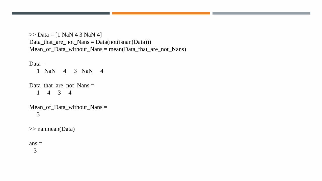
>> Data = [1 NaN 4 3 NaN 4]

Data_that_are_not_Nans = Data(not(isnan(Data)))

Mean_of_Data_without_Nans = mean(Data_that_are_not_Nans)

Data =

1 NaN 4 3 NaN 4

Data_that_are_not_Nans =

1 4 3 4

Mean_of_Data_without_Nans =

3

>> nanmean(Data)

ans =

3

Calculating with matrices

Rounding values

>> A = [1 2.6 2.4 1.3 5.0;4.8 2.2 3.6 1.4 2]

A =

1.0000 2.6000 2.4000 1.3000 5.0000

4.8000 2.2000 3.6000 1.4000 2.0000

>> round(A)

ans =

1 3 2 1 5

5 2 4 1 2

>> floor(A)

ans =

1 2 2 1 5

4 2 3 1 2

>> ceil(A)

ans =

1 3 3 2 5

5 3 4 2 2

>> fix(A)

ans =

1 2 2 1 5

4 2 3 1 2

Difference between floor, ceil, and fix??

Generate a set of 1000 scores (satscores) in a 100×10 table that are normally distributed as ideal SAT scores

(mean 500, sd = 100). Verify that the mean and standard deviation of each column are near 500 and 100,

respectively. Draw the histogram of the satscores.

Make a random integer vector M that follows a uniform distribution. M should have 100 members (1 row and 100

columns or 1 column and 100 rows). Minimum value should be 1 and maximum value should be 100. Draw 20

values randomly from the M, and obtain mean and standard deviation of the 20 values. Also get mean and standard

deviation of the vector M.

Create SATs, a 1400 ×2 matrix of normally distributed random multiples of 10 (i.e. 200, 210, 220, etc.) with a

mean of 500 and a standard deviation of 100, using randn, round, and other operations. Find the mean and standard

deviation of each column (use round or ceil or floor function).

EXERCISE, ASSIGNMENTS FOR THE NEXT CLASS

EXERCISE

Type load(‘mathScores.mat’): please download ‘mathScores.mat’ file from the course website. The file has math scores of three classes. Size of each class is 100. Some people did not take the exam, and those missing values were replaced by NaNs.

1) Get mean and standard deviation of each class’s math score. Also get grand mean and standard deviation of all the math scores.

2) Find how many people did not take exam.

3) The instructor decided to give -10 point to the people who did not take exam. Replace all the NaNs with -10 and make a new matrix called ‘newScores’. What is mean and standard deviation of the ‘newScores’?

4) Draw histograms of math scores (old and new). Distinguish each class data with different colors.

You should use ‘bar’ function for drawing histogram and changing colors. [n, x] = hist(newScores(:,1), 10); h = bar(x, n);set(h, ‘facecolor’, [1 0 0]);

SOME BUILT-IN FUNCTIONS FOR

CALCULATIONS

Built in functions>> m = 64

m =

64

>> q = sqrt(m)

q =

8

>> pi

ans =

3.1416

>> remPiOver3 = rem(pi,3)

remPiOver3 =

0.1416

>> rem(7,2)

ans =

1

>> rem(8,3)

ans =

2

>> abs([-1 2 -3 4])

ans =

1 2 3 4

>> exp(1)

ans =

2.7183

>> exp(2)

ans =

7.3891

What about log5??

>> log5(625)

Undefined function 'log5' for input

arguments of type

'double'.

Did you mean:

>> log(625)/log(5)

ans =

4

Built in functions

>> log(1)

ans =

0

>> log(2)

ans =

0.6931

>> log2of_128 = log2(128)

log2of_128 =

7

>> two_tothe_7 = 2^7

two_tothe_7 =

128

>> log10of_1000 = log10(1000)

log10of_1000 =

3

>> ten_tothe_3 = 10^3

ten_tothe_3 =

1000

>> ten_tothe_3 = 1000

ten_tothe_3 =

1000

Imaginary number

Built in functions

ROTATION MATRIX

%rotateScript1.m

R = [cos(pi/6) -sin(pi/6);sin(pi/6) cos(pi/6)];

originalradiuspoint = [1;0];

radiusrotatedOnce = R*originalradiuspoint;

radiusrotatedFourMoreTimes = R^4 * radiusrotatedOnce;

figure(1)

plot([0 originalradiuspoint(1)], [0 originalradiuspoint(2)], 'k');

hold on

plot([0 radiusrotatedOnce(1)], [0 radiusrotatedOnce(2)], 'b');

plot([0 radiusrotatedFourMoreTimes(1)], [0 radiusrotatedFourMoreTimes(2)], 'r');

axis square;

grid on;

set(gca, 'xlim', [-1 1], 'ylim', [-1 1], 'tickdir', 'out')

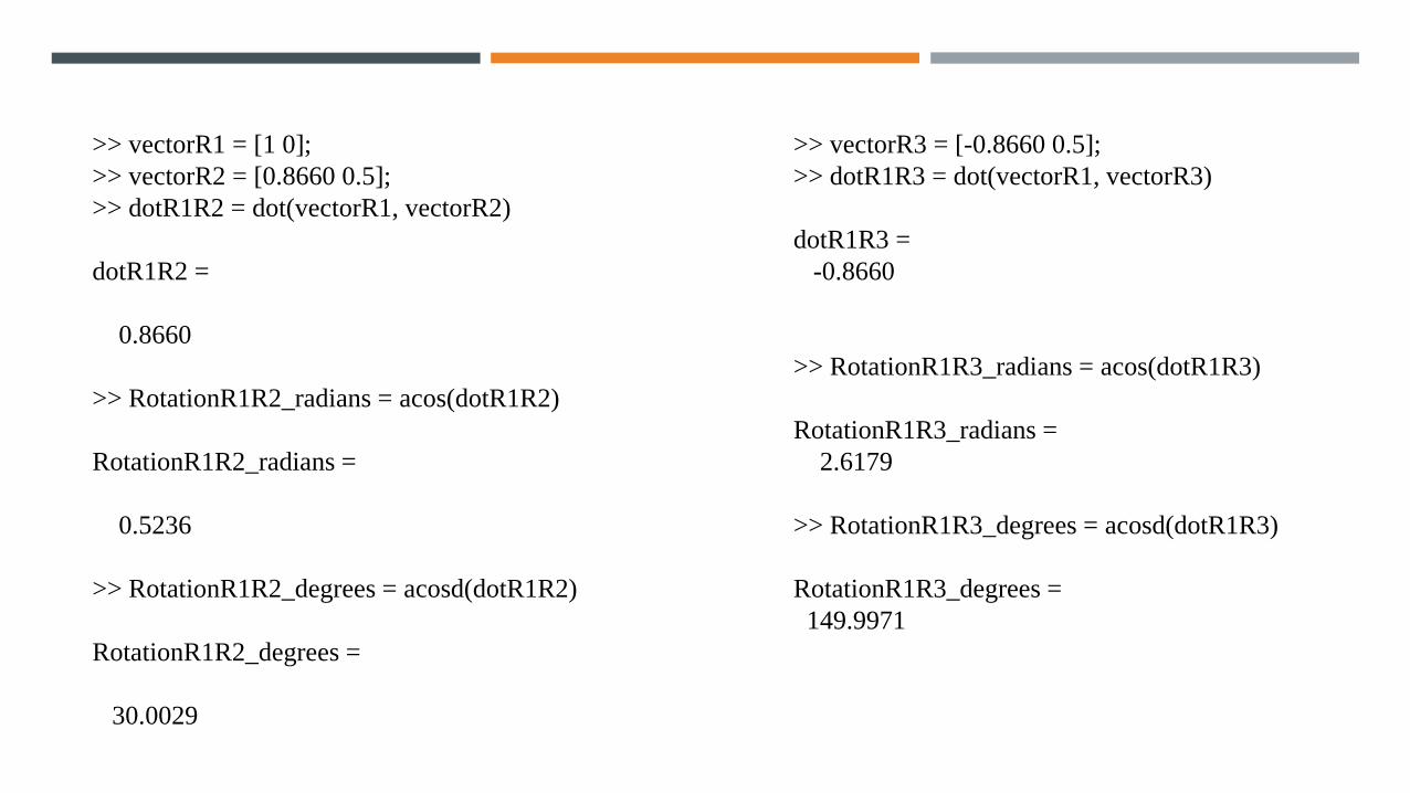
>> vectorR1 = [1 0];

>> vectorR2 = [0.8660 0.5];

>> dotR1R2 = dot(vectorR1, vectorR2)

dotR1R2 =

0.8660

>> RotationR1R2_radians = acos(dotR1R2)

RotationR1R2_radians =

0.5236

>> RotationR1R2_degrees = acosd(dotR1R2)

RotationR1R2_degrees =

30.0029

>> vectorR3 = [-0.8660 0.5];

>> dotR1R3 = dot(vectorR1, vectorR3)

dotR1R3 =

-0.8660

>> RotationR1R3_radians = acos(dotR1R3)

RotationR1R3_radians =

2.6179

>> RotationR1R3_degrees = acosd(dotR1R3)

RotationR1R3_degrees =

149.9971

load('eyeData.mat');

R = [cos(pi/4) -sin(pi/4);sin(pi/4) cos(pi/4)];

newEyeH = [];

newEyeV = [];

for i = 1:size(hComp, 1)

currEye = [hComp(i,:);vComp(i,:)];

rotEye = R*currEye;

newEyeH = [newEyeH;rotEye(1,:)];

newEyeV = [newEyeV;rotEye(2,:)];

end

plot(transpose(hComp), transpose(vComp), 'k') ;

hold on

set(gca, 'xlim', [-12 12], 'ylim', [-12 12], 'tickdir', 'out');

plot([-12 12], [0 0], 'k:');

plot([0 0], [-12 12], 'k:');

plot(transpose(newEyeH), transpose(newEyeV), 'r');

axis square;

ROTATING EYE VELOCITY

EXERCISE

▪ Rotate the ‘hComp, vComp’ 90 degrees counter-clockwise and plot them in blue color.

▪ Rotate the ‘hComp, vComp’ 180 degrees clockwise and plot them in green color.

▪ Make two subplots (subplot(2,1,1) and subplot(2,1,2)). Plot the rotated horizontal components in the

first subplot, and the rotated vertical components in the second subplot. Make the ‘ylim’ of the two

plots the same ([0 10]). Put labels in x and y axis (‘time (ms)’, and ‘velocity (deg/s)’). Put title of the

figure (title should be ‘Rotated eye velocity components’).