Getting Maps and Plotting Data on a MapJuly 30, 2007

Sections with asterisks (*) are optional and only covered if time allows.

In this tutorial we will learn several things. By the end of this tutorial you should be able to

• Find and download a map from the ESRI site.

• Identify which layers are appropriate for use in your analysis.

• Look at a ArcGIS shapefile without having to import it into GRASS.

• Import a shapefile into GRASS.

• Perform maintenance on an image so that GRASS can use it correctly.

• Save your work for future use.

• Plot data points onto the downloaded map.

• Vary attributes of the points based on the data.

Using Maps from ESRI*

The company that markets ArcGIS has a very large site containing maps and shapefiles that canbe included in your GRASS maps. For this tutorial we will use Census 2000 TIGER/Line Datawhich can be found at

http://www.esri.com/data/download/census2000 tigerline/index.html

There are many other datasets on this site that you should explore at some point. The free datasetscan be found at the Geography Portal at

http://www.esri.com/data/resources/geographic-data.html

To get started, click on the Preview and Download link in left hand side of the page.

In the next step, you will select a state for which you want data. Select California and hitnext.

Then select the California county that you want data for. Select Santa Barbara and click theSubmit Selection button below the Select by County drop down menu. Note that if you want

1

data for all of California and not just a particular county, you can select a data layer from theSelect by Layer menu.

You are now taken to a long list of available data layers available as shapefiles. For this tutorialcheck off the following boxes:

• County 2000 contains the boundaries of the county we have selected. It is important tonote that the boundaries denote all area owned by the county including coastline and oceanout to a certain depth or distance.

• Line Features - Roads contains all roads and highways in the queried county. We alsohave access to the attribute table that lists the road names.

• Urban Areas 2000 contains the locations of the areas in the queried county designated asurban areas according to the 2000 US Census. An attribute table includes the names of theseareas. As an exercise, we will plot the names of these cities.

• Water Polygons contain the area in the queried county that are designated as bodies ofwater. These include not only rivers, streams and lakes, but also the section of the oceanthat belongs to the county.

Once you have selected these layers, click on Proceed to Download then click on Download Fileon the resulting screen. This will download a ZIP file to your default downloads location. On Mac,locate the file and double-click it to extract its contents to the same directory. On Windows XPand Vista you can double click the zip file but you will need to extract the contents manually. Onprevious versions of Windows you will need a zip client such as WinZip or WinRAR to extract thecontents of the file.

NOTE: The filename of the zip archive and the extracted directory may differ from what ispictured in this document. That is no problem.

2

Notice that the names of the directories are rather cryptic. There is a system for how ESRI namesits TIGER files, and it can be found in the readme.html file. For brevity, the table below mapsthe directory name with the list of layers on the previous page.

Directory Name Format Description of Contentscty00xxxxx County 2000IkAxxxxx Line Features - Roadsurb00ccccc Urban Areas 2000watxxxxx Water Polygons

xxxxx represents the unique code used to identify the particular county we queried. This code forSanta Barbara County is 06083.

Within each of these directories, one will find several files. We will only deal with the files with.shp extension.

3

Looking at the Shapefiles*

Using an application called QGIS, we can look at what each shapefile contains and how severallayers look when plotted together. QGIS is a great tool for exploring data within shapefiles withouthaving to import them into GRASS first. You can download QGIS at http://www.qgis.org.QGIS is not necessary to follow along in this section. We can also use QGIS to rearrangeand modify layers, but I will not discuss that.

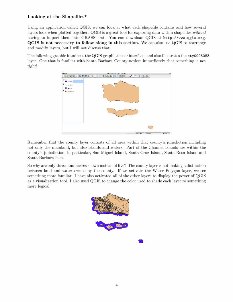
The following graphic intoduces the QGIS graphical user interface, and also illustrates the cty0006083layer. One that is familiar with Santa Barbara County notices immediately that something is notright!

Remember that the county layer consists of all area within that county’s jurisdiction includingnot only the mainland, but also islands and waters. Part of the Channel Islands are within thecounty’s jurisdiction, in particular, San Miguel Island, Santa Cruz Island, Santa Rosa Island andSanta Barbara Islet.

So why are only three landmasses shown instead of five? The county layer is not making a distinctionbetween land and water owned by the county. If we activate the Water Polygon layer, we seesomething more familiar. I have also activated all of the other layers to display the power of QGISas a visualization tool. I also used QGIS to change the color used to shade each layer to somethingmore logical.

4

We can now see each of the distinct islands as well as the water features in Santa Barbara Countyincluding a lake and a river. The urban areas are shaded in lavender and the network of roads arelight grey.

Preparing to Import a Shapefile

First we need to create a new location and mapset. Refer to previous tutorials for instructions onhow to do this. Below I provide the parameters I use for the location using the command g.region-p. Note that it is incredibly easy to get these parameters using QGIS.

Important! The output below displays the fractional part of latitude and longitude using minutes.To convert back to decimals, divide the number after the colon (:) by 60. Add a negative sign infront of the west and east benchmarks since this data is in the western hemisphere.

projection: 3 (Latitude-Longitude)zone: 0datum: nad83ellipsoid: grs80north: 35:12N (35.2)south: 33:18N (33.3)west: 120:48W (-120.8)east: 119:24W (-119.4)nsres: 0:00:06.84 (.0019)ewres: 0:00:05.04 (.0014)rows: 1000cols: 1000cells: 1000000

When asked if you wish to enter a specific datum, answer y and enter nad83. Whenasked to enter a transformation, enter 1. These parameters are specific to the filesthat you are using and may not translate to your particular situation.

For the default region, enter the values in parentheses above, then create a new mapset.

5

Importing the Shapefiles into GRASS

In the newly created location and mapset, type v.in.ogr. The following screen displays.

In OGR datasource name enter the path to the shapefile you wish to import. You can browse tothe file by clicking on the file folder icon. In the Name for output vector map enter a name forthe vector map.

Try running this. If you get an error about projections not matching and you are sure the projectionsdo in fact match, select Override dataset projection (use location’s projection). In myparticular case, I do get this error, but I know that the projections do match.

Now let’s do the same for the Roads and Cities layers.

Next, activate the GIS manager and click on the button circled in red to Add a Vector Layer.If the GIS manager is not displaying, type gis.m in the GRASS shell.

6

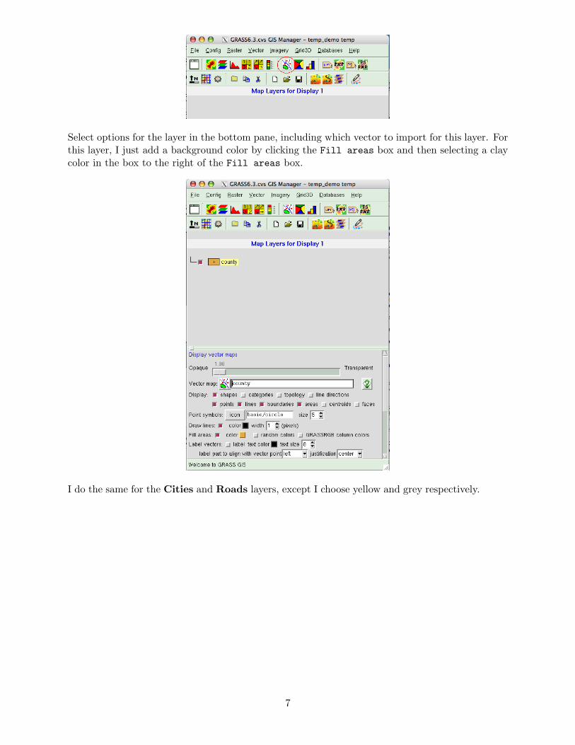
Select options for the layer in the bottom pane, including which vector to import for this layer. Forthis layer, I just add a background color by clicking the Fill areas box and then selecting a claycolor in the box to the right of the Fill areas box.

I do the same for the Cities and Roads layers, except I choose yellow and grey respectively.

7

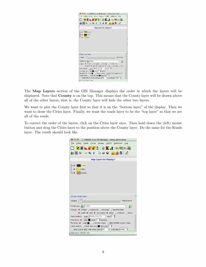
The Map Layers section of the GIS Manager displays the order in which the layers will bedisplayed. Note that County is on the top. This means that the County layer will be drawn aboveall of the other layers, that is, the County layer will hide the other two layers.

We want to plot the County layer first so that it is on the “bottom layer” of the display. Then wewant to draw the Cities layer. Finally, we want the roads layer to be the “top layer” so that we seeall of the roads.

To correct the order of the layers, click on the Cities layer once. Then hold down the (left) mousebutton and drag the Cities layer to the position above the County layer. Do the same for the Roadslayer. The result should look like

8

Now click over to the Map Display window and click on icon circled in red. You can hide layersin this map by clicking on the red box next to the layer you want to hide in the GIS Manager.Each time you make a change though, you must refresh the map display window by clicking onthat icon circled in red.

And VOILA! The following map should appear.

Saving your Work

Up to this point we have done a lot of work. In subsequent GRASS sessions we are going to wantto start from where we left off. We can save our work in GIS Manager.

To save your work, activate the GIS Manager and click on the File menu. Click on Workspaceand then slide over to Save.

During the next GRASS session, we can reload our work by bringing down the File menu. Clickon Workspace and then slide over and click on Open.

9

Plotting Data on the Map

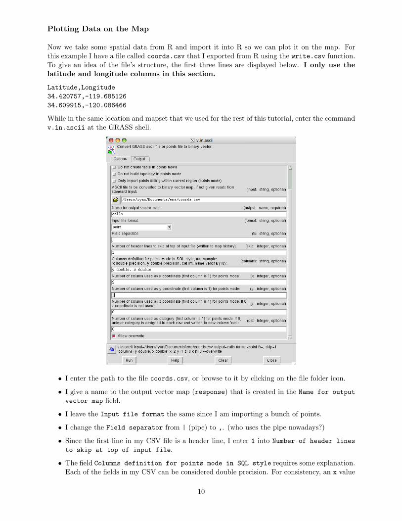
Now we take some spatial data from R and import it into R so we can plot it on the map. Forthis example I have a file called coords.csv that I exported from R using the write.csv function.To give an idea of the file’s structure, the first three lines are displayed below. I only use thelatitude and longitude columns in this section.

Latitude,Longitude34.420757,-119.68512634.609915,-120.086466

While in the same location and mapset that we used for the rest of this tutorial, enter the commandv.in.ascii at the GRASS shell.

• I enter the path to the file coords.csv, or browse to it by clicking on the file folder icon.

• I give a name to the output vector map (response) that is created in the Name for outputvector map field.

• I leave the Input file format the same since I am importing a bunch of points.

• I change the Field separator from | (pipe) to ,. (who uses the pipe nowadays?)

• Since the first line in my CSV file is a header line, I enter 1 into Number of header linesto skip at top of input file.

• The field Columns definition for points mode in SQL style requires some explanation.Each of the fields in my CSV can be considered double precision. For consistency, an x value

10

is a longitude value and a y value is a latitude value. The first field in my file is latitude(y) and the second is longitude (x). I tell GRASS this by entering the following: y doubleprecision, x double precision.

• I enter 2 for Number of column used as x coordinate since the second field is longitudewhich is an x value.

• Similarly, I enter 1 for Number of column used as y coordinate.

• Since my data is only two-dimensional (there is no elevation component), I enter 0 for Numberof column used as z coordinate because there is no z coordinate.

• I also do not have a category column, so I enter 0 there as well.

Now move back to the GIS Manager and add a new vector layer for the vector calls. Move thecalls layer to the top so it will be displayed above all other layers. It is also wise to disable theroads layer so we can see the points more clearly.

Let’s customize the points a bit. Select a fill color for the points in Fill area. I have selected red.Let’s also change the Point symbols marker to something else by clicking on the icon button. Ichose basic/triangle. Let’s also change the size field to 5.

11

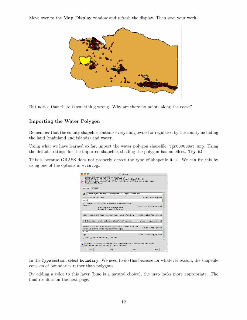
Move over to the Map Display window and refresh the display. Then save your work.

But notice that there is something wrong. Why are there no points along the coast?

Importing the Water Polygon

Remember that the county shapefile contains everything owned or regulated by the county includingthe land (mainland and islands) and water.

Using what we have learned so far, import the water polygon shapefile, tgr06083wat.shp. Usingthe default settings for the imported shapefile, shading the polygon has no effect. Try it!

This is because GRASS does not properly detect the type of shapefile it is. We can fix this byusing one of the options in v.in.ogr.

In the Type section, select boundary. We need to do this because for whatever reason, the shapefileconsists of boundaries rather than polygons.

By adding a color to this layer (blue is a natural choice), the map looks more appropriate. Thefinal result is on the next page.

12

13