getting started with simulink: an introductory tutorial · an introductory tutorial: ... es205...

ES205 Getting started with Simulink of 16

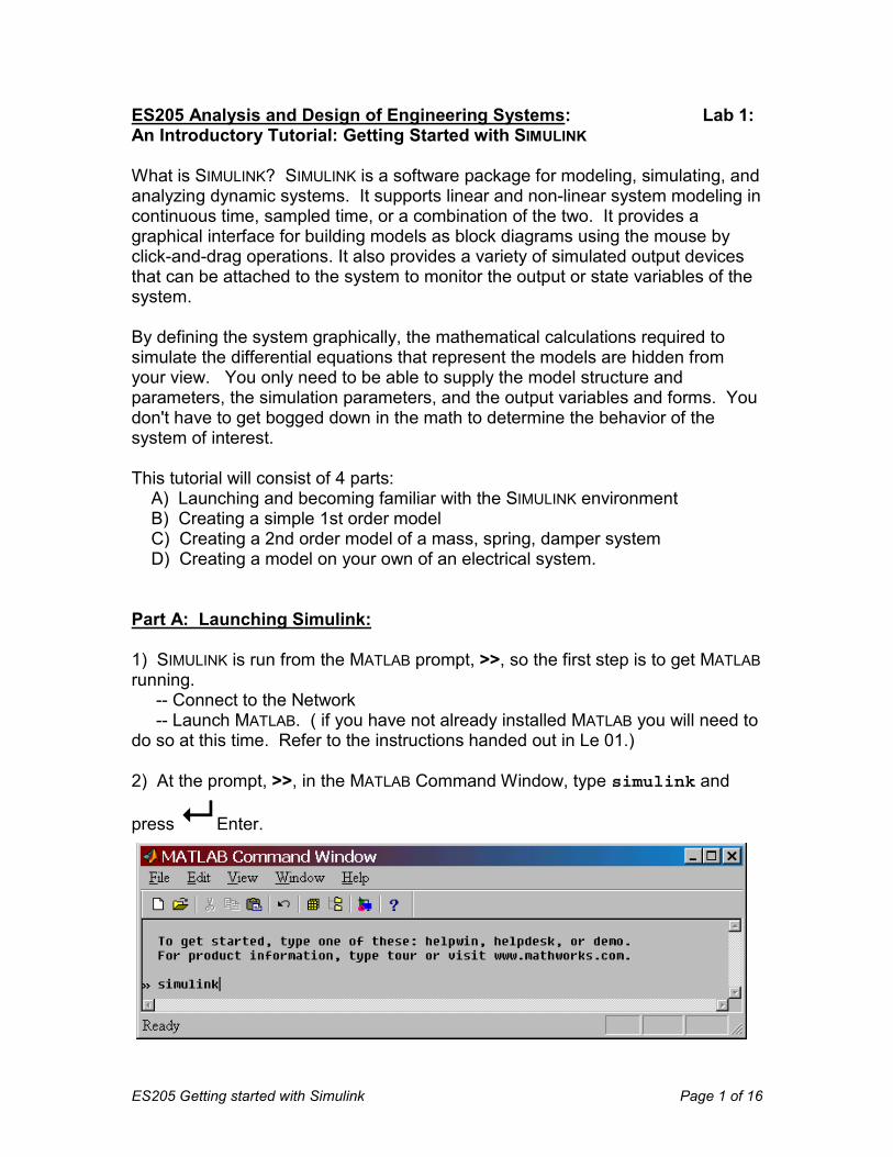
ES205 Analysis and Design of Engineering Systems: Lab 1: An Introductory Tutorial: Getting Started with SIMULINK What is SIMULINK? SIMULINK is a software package for modeling, simulating, and analyzing dynamic systems. It supports linear and non-linear system modeling in continuous time, sampled time, or a combination of the two. It provides a graphical interface for building models as block diagrams using the mouse by click-and-drag operations. It also provides a variety of simulated output devices that can be attached to the system to monitor the output or state variables of the system. By defining the system graphically, the mathematical calculations required to simulate the differential equations that represent the models are hidden from your view. You only need to be able to supply the model structure and parameters, the simulation parameters, and the output variables and forms. You don't have to get bogged down in the math to determine the behavior of the system of interest. This tutorial will consist of 4 parts: A) Launching and becoming familiar with the SIMULINK environment B) Creating a simple 1st order model C) Creating a 2nd order model of a mass, spring, damper system D) Creating a model on your own of an electrical system. Part A: Launching Simulink: 1) SIMULINK is run from the MATLAB prompt, >>, so the first step is to get MATLAB running. -- Connect to the Network -- Launch MATLAB. ( if you have not already installed MATLAB you will need to do so at this time. Refer to the instructions handed out in Le 01.) 2) At the prompt, >>, in the MATLAB Command Window, type simulink and

press ! Enter.

ES205 Getting started with Simulink

3) When SIMULINK opens you will see the box called the SIMULINK Library Browser. The Library consist of a number of different SIMULINK blocks with which a system model may be built. To build a model, you first need to create a space to make the model. Click the new model icon in the upper left corner to open a new SIMULINK file workspace. Next, select the SIMULINK icon to expand the list of the available elements that are used to create a system model. 4) After making the selections in Step 3, the SIMULINK Library Browser will show folders that contain the most commonly used elements you will be using for model creation. Click on each of the following folders and quickly note the elements that are contained in each. -- Continuous -- Discrete -- Functions & Tables -- Math -- Nonlinear -- Signals & Systems -- Sinks -- Sources When needed, these elements may simply be clicked, dragged, and dropped into the model workspace.

of 16

ES205 Gettin

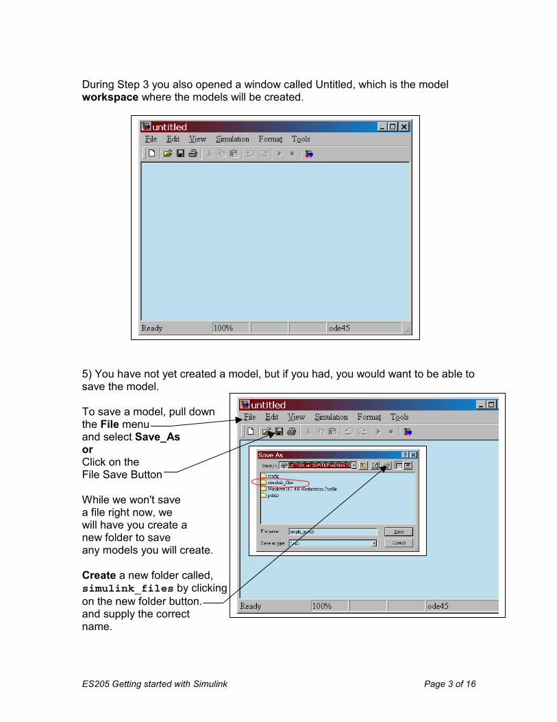
During Step 3 you also opened a window called Untitled, which is the model workspace where the models will be created. 5) You havsave the m To save a the File meand select or Click on thFile Save B While we wa file right will have ynew folderany model Create a nsimulinkon the newand supplyname.

g started with Simulink

e not yet created a model, but if you had, you would want to be able to odel.

model, pull down nu Save_As

e utton

on't save now, we ou create a to save s you will create.

ew folder called, _files by clicking o folder button. the correct

n

of 16

ES20

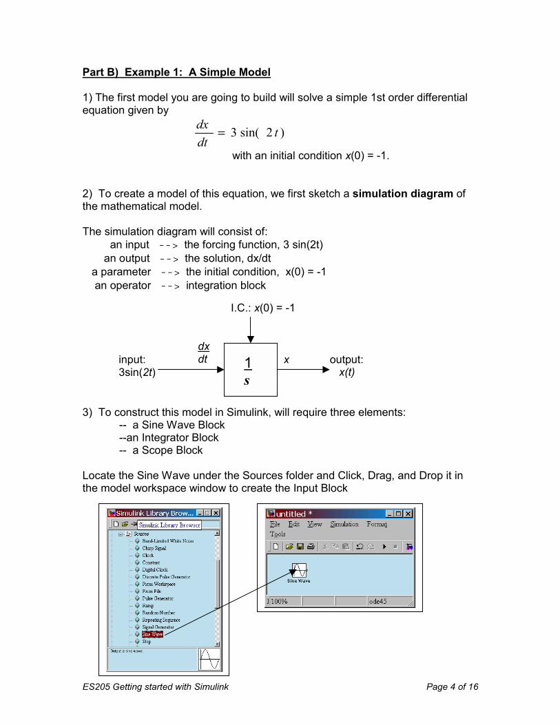
Part B) Example 1: A Simple Model 1) The first model you are going to build will solve a simple 1st order differential equation given by

)2sin(3 tdtdx =

with an initial condition x(0) = -1. 2) To create a model of this equation, we first sketch a simulation diagram of the mathematical model. The simulation diagram will consist of: an input --> the forcing function, 3 sin(2t) an output --> the solution, dx/dt a parameter --> the initial condition, x(0) = -1 an operator --> integration block 3) To construct this model in Simulink, will require three elements: -- a Sine Wave Block --an Integrator Block -- a Scope Block Locate the Sine Wave under the Sources folder and Click, Drag, and Drop it in the model workspace window to create the Input Block

output: x(t)

x dx dt input:

3sin(2t)

I.C.: x(0) = -1

1 s

5 Getting started with Simulink
of 16

ES

4) Locate the Integrator under the Continuous folder and Click, Drag, and Drop it in the model workspace window to create the Operator Block. 5) mo

205 Getting started with Simulink

Locate the Scope under the Sinks folddel workspace window to create the O

er and Click, Drag, and Drop it in the utput Block

of 16

ES205 G

6) Connecting the blocks. Blocks can be connected by dragging a line from the output of one block to the input of another block. Make the following connections: Output of the Sine Wave --> Input of the Integrator Output of the Integrator --> Input of the Scope The ar 7) Sel Most bthe pardialog Doubleand se Am Fre

etting started with Simulink

rows indicate the direction of the signal flow.

ecting Simulation Parameters.

locks have different parameters that are associated with them. To access ameters, simply double-click on the block of interest. This will bring up a box which allows the parameters to be changed.

click on the Sine Wave t the following parameters:

plitude = 3 quency = 2

of 16


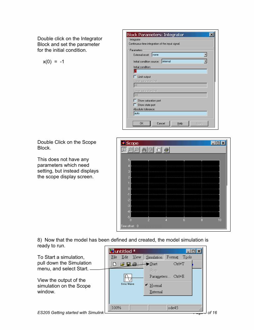
Double click on the Integrator Block and set the parameter for the initial condition. x(0) = -1 Double Click on the Scope Block. This does not have any parameters which need setting, but instead displays the scope display screen. 8) Now that the model has been defineready to run. To Start a simulation, pull down the Simulation menu, and select Start. View the output of the simulation on the Scope window.

of 16

d and created, the model simulation is


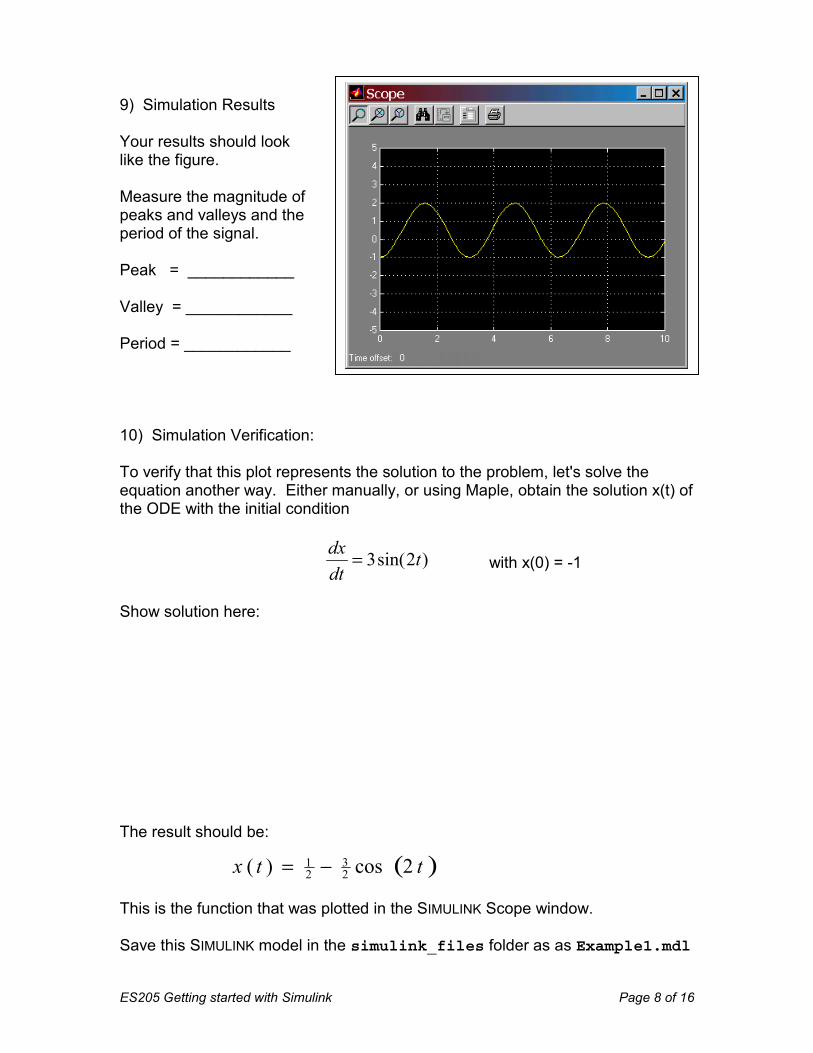
9) Simulation Results Your results should look like the figure. Measure the magnitude of peaks and valleys and the period of the signal. Peak = ____________ Valley = ____________ Period = ____________ 10) Simulation Verification: To verify that this plot represenequation another way. Either mthe ODE with the initial conditio

dd

Show solution here: The result should be:

This is the function that was plo Save this SIMULINK model in th

tx )( 21 −=

of 16

ts the solution to the problem, let's solve the anually, or using Maple, obtain the solution x(t) of n

)2sin(3 ttx = with x(0) = -1

tted in the SIMULINK Scope window.

e simulink_files folder as as Example1.mdl

( )t2cos23


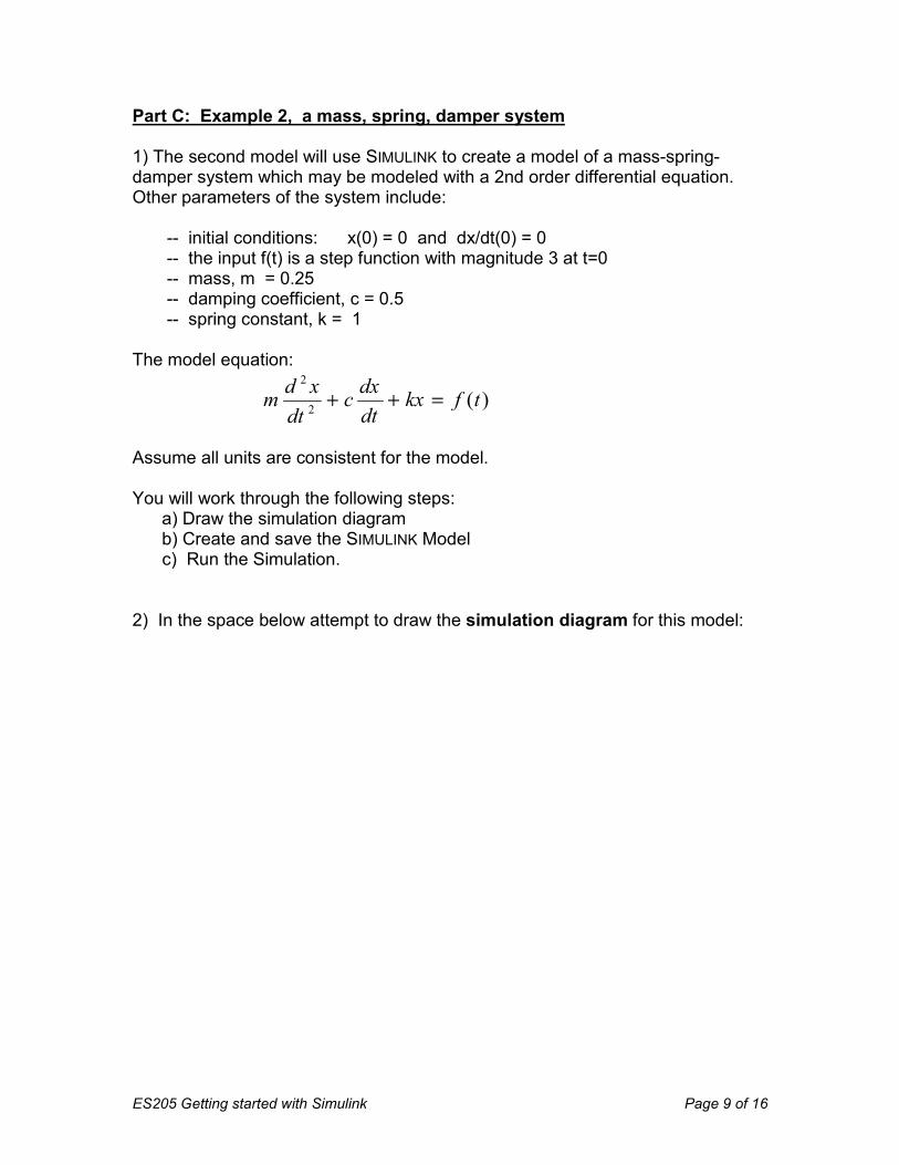
Part C: Example 2, a mass, spring, damper system 1) The second model will use SIMULINK to create a model of a mass-spring-damper system which may be modeled with a 2nd order differential equation. Other parameters of the system include: -- initial conditions: x(0) = 0 and dx/dt(0) = 0 -- the input f(t) is a step function with magnitude 3 at t=0 -- mass, m = 0.25 -- damping coefficient, c = 0.5 -- spring constant, k = 1 The model equation:

)(2

2

tfkxdtdxc

dtxdm =++

Assume all units are consistent for the model. You will work through the following steps: a) Draw the simulation diagram b) Create and save the SIMULINK Model c) Run the Simulation. 2) In the space below attempt to draw the simulation diagram for this model:

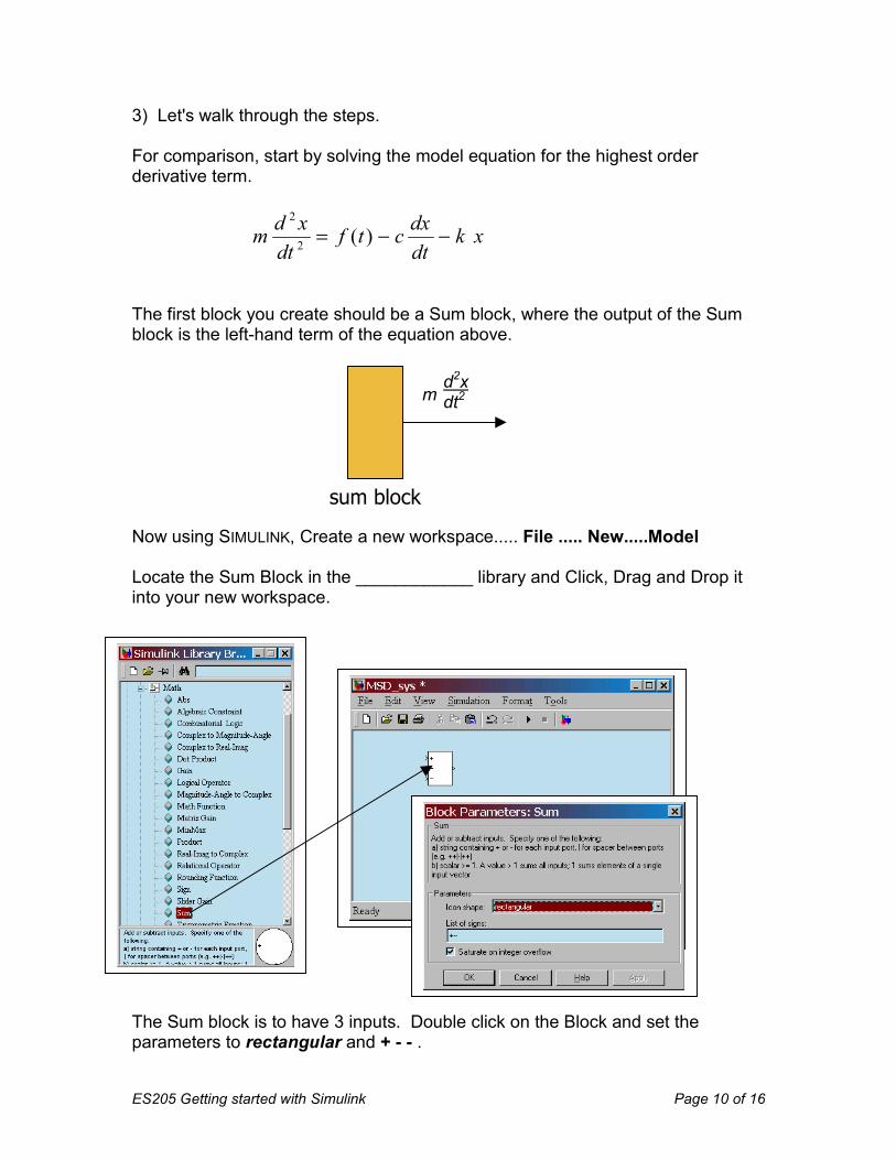
3) Let's walk through the steps. For comparison, start by solving the model equation for the highest order derivative term.

xkdtdxctf

dtxdm −−= )(2

2

The first block you create should be a Sum block, where the output of the Sum block is the left-hand term of the equation above. Now using SIMULINK, Create a new workspace..... File ..... New.....Model Locate the Sum Block in the ____________ library and Click, Drag and Drop it into your new workspace.

sum block

m d2x dt2

ES205 Getting started with Simu

The Sum block is to have 3parameters to rectangular

link

inputs. D and + - -

of 16

ouble click on the Block and set the .

4) Gain Block. Add a gain (multiplier) block to normalize the coefficient, m, to modify the signal so it is equal to the highest order derivative term alone. Click, Drag, and Drop a Gain Block from the _____________ library into the SIMULINK workspace.

m d2x

dt2 1 m

d2x dt2

sum block gain


Double-click on the Gain block to Use a Gain of _______________ Add a title to the Gain Block.

change

____

of 16

the block parameters.


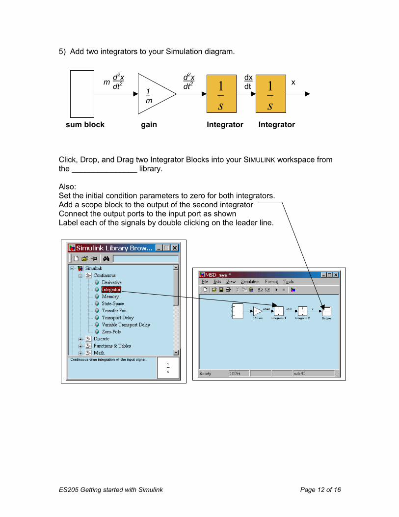
5) Add two integrators to your Simulation diagram. Click, Drop, and Drag two Integrator Blocks into your SIMULINK workspace from the _______________ library. Also: Set the initial condition parameters to zero for both integrators. Add a scope block to the output of the second integrator Connect the output ports to the input port as shown Label each of the signals by double clicking on the leader line.

m d2x

dt2 1 m

d2x dt2

sum block gain

s1

s1

dx dt x

Integrator Integrator

of 16

6) Return Branch Gain Blocks In the Simulation Diagram, connect the integrated signals with gain blocks to create the terms on the right-hand side of the model equation. In SIMULINK, Drag in two additional Gain blocks from the Math library to the workspace. --Flip these blocks by selecting each block and using...... Format.......Flip Block --Double click on each of the blocks and set the appropriate parameters c = 0.5 k = 1.0 --Connect the signal lines: Either Click the gain block input and drag to each of the branch points. or Ctrl-Click to select the branch point first and drag to the gain inputs. --Add appropriate titles to the gain blocks

m d2x

dt2 1 m

d2x dt2

sum block

s1

s1

k

c dx dt

k x

c

dx dt x


5

0
k = 1.
c = 0.

of 16

7) Connect all Input Signals. In the Simulation Diagram, connect all the input signals to the appropriate inputs of the Sum Block. In the SIMULINK workspace: -- Add a Step Block from the Source library and set its parameters. Step time = 0 Initial value = 0 Final value = 3 -- Connect the signal lines to the sum Block, paying attention to the signs of the inputs.

m d2x

dt2 1 m

d2x dt2

s1

s1

k

c dx dt

k x

c

dx dt x

+ - -

Input: f(t) Output:

x(t)

of 16


8) Your completed SIMULINK model should look like the following. Complete any missing titles or labels. Save your model as Example2.mdl 9) Running your simulation Double click on the Scope to make its output visible. Run your simulation. What is it maximum value of x reached?______________ What is its final value of x reached?__________________ Is this behavior underdamped, overdamped, or critically damped?


This concludes the SIMULINK Tutorial Module. You are now to complete Part D: Lab 1 Worksheet. To complete the worksheet you are expected to understand and use the terms below. Terms used on the worksheet: Steady State Value is the final value of the system settles at after transient behavior has dissipated. Overshoot is characterized as the maximum response swing past the steady state value. Rise time is time required for the system to rise from ten to ninety percent of the steady state value. Settling time is the amount of time the system takes to value settle close to the steady state condition (to within approximately 2% of the step size).

.

Rise Time

+/- 2% of step

Settling Time

Overshoot

Steady State Value

ES205 Lab 1 Worksheet Page 1 of 6

Name __________________________Section _______ C M _____________ Lab Partners: ________________ __________________ _______________ Part D: Lab 1 Worksheet ES205 Analysis and Design of Engineering Systems 1) Mass-Spring-Damper Model: Below you will explore how changing each of the three parameters, m, c, and k , affect the system response of the spring-mass-damper model created in Part C. Varying the mass, m: In the space below, make a prediction. How do you think changing the mass, m, of the system will affect its dynamic behavior? Now using your SIMULINK model, vary the value of the mass, m, using the multipliers given below, while keeping k and c constant. Then on the graph below sketch and label each response. Use Mass values: m/5 m/2 1.0*m 2.0*m and 5*m

Summary: Give a short summary which qualitatively describes how changing the mass affected the system response. Include qualitative reference to the overshoot, settling time, and steady state value.


Varying the damping constant, c: Make another prediction. How will changing the damping constant, c, of the system affect its dynamic behavior? Now using your SIMULINK model, vary the value of the mass, c, using the multipliers given below, while keeping k and m constant. Then on the graph below sketch and label each response. Use Damping Constants: c/5 c/2 1.0*c 2.0*c and 5*c

Summary: Give a short summary which qualitatively describes how changing the damping constant affects the system response. Include qualitative reference to the overshoot, settling time, and steady state value.


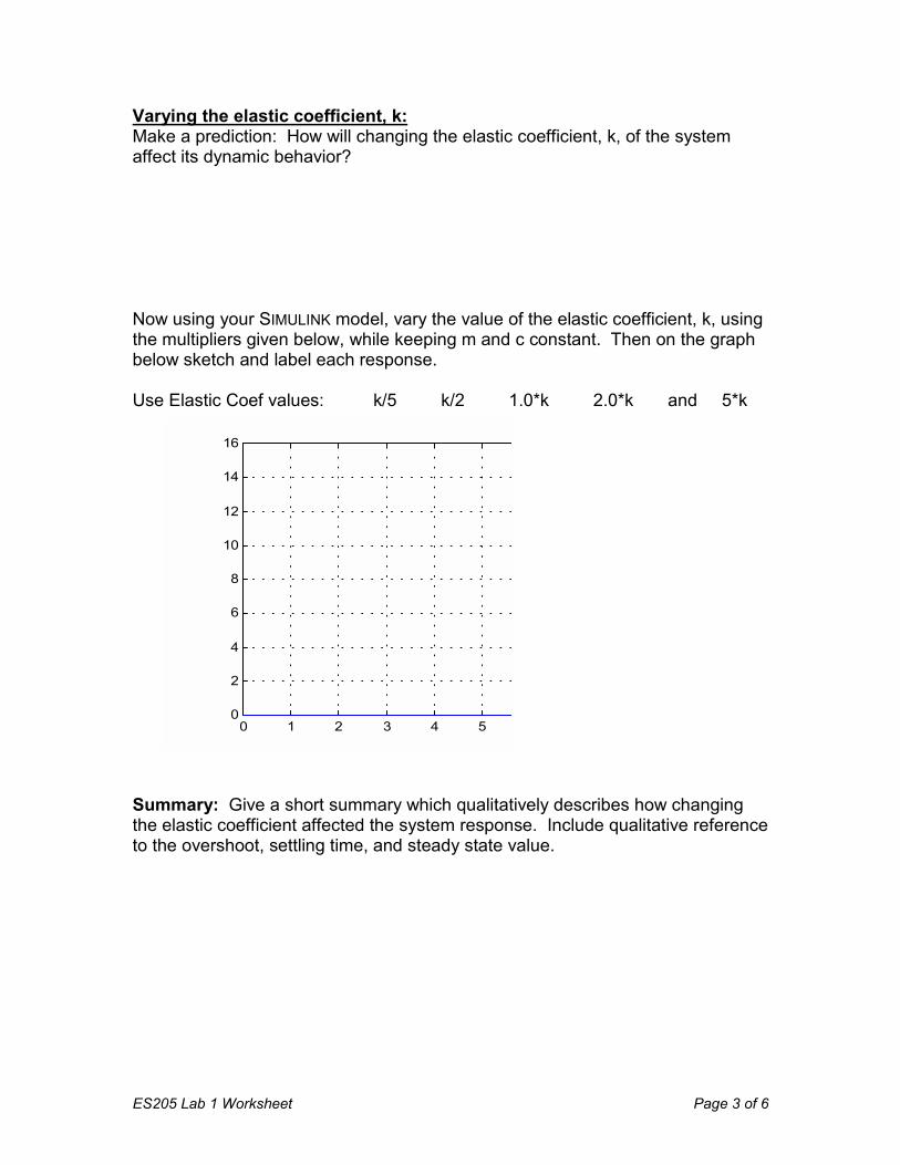
Varying the elastic coefficient, k: Make a prediction: How will changing the elastic coefficient, k, of the system affect its dynamic behavior? Now using your SIMULINK model, vary the value of the elastic coefficient, k, using the multipliers given below, while keeping m and c constant. Then on the graph below sketch and label each response. Use Elastic Coef values: k/5 k/2 1.0*k 2.0*k and 5*k

Summary: Give a short summary which qualitatively describes how changing the elastic coefficient affected the system response. Include qualitative reference to the overshoot, settling time, and steady state value.

0 1 2 3 4 50

2

4

6

8

10

12

14

16

ES205 Lab 1 Worksheet

2) Modeling a Simple Electrical RLC Circuit. A simple electrical circuit consists of a Resistor, Coil, and Capacitor in series with a variable voltage source, E(t). The circuit may be modeled using tw

1 1 ( )di R i e E t

dt L L L+ + =

with i(0) = 0 where i is the current in the circuit anbetween the coil and capacitor. Draw the Simulation Diagram that re

R L

E(t)

-

e

i

C
+
Page 4 of 6

o 1st order DE's given as

and 1 0de i

dt C− =

with e(0) = 0

d e is the electric potential at the node

presents these DEs below.


Now using your Simulation diagram, create the SIMULINK model for this electrical system using the values: R = 3 L = 1 C =0.5 and E(t), which is a pulse defined as Add Scope Blocks to display both outputs, i and e, as well as the input voltage, E(t). Make sure you include appropriate labeling of the blocks, signals, and I/O. Run the simulation for 0< t < 10 Sketch the shape of the output signals below: Now experiment with your model by varying each of the component parameters, R, L, and C. Describe the effect each has on the system response. Effect of Varying R: Effect of Varying L: Effect of Varying C:

E(t) 2

t 1 5

e

t t

i


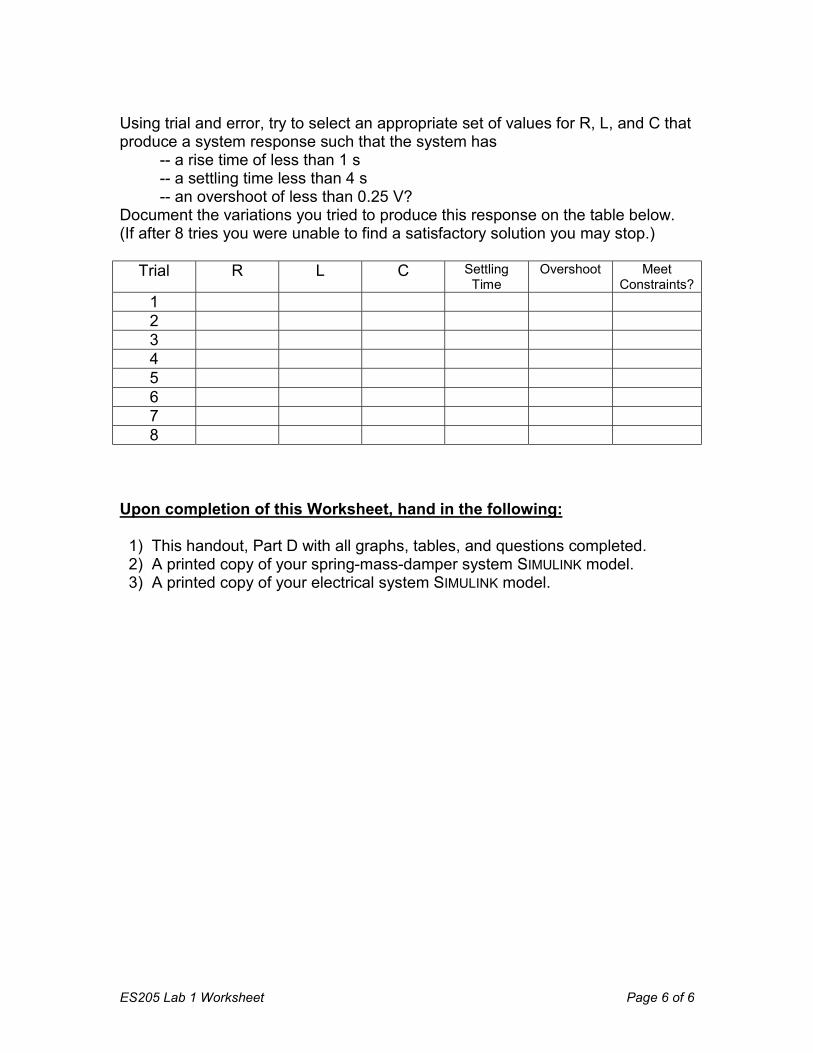
Using trial and error, try to select an appropriate set of values for R, L, and C that produce a system response such that the system has -- a rise time of less than 1 s -- a settling time less than 4 s -- an overshoot of less than 0.25 V? Document the variations you tried to produce this response on the table below. (If after 8 tries you were unable to find a satisfactory solution you may stop.)

Trial R L C Settling Time

Overshoot Meet Constraints?

1 2 3 4 5 6 7 8

Upon completion of this Worksheet, hand in the following: 1) This handout, Part D with all graphs, tables, and questions completed. 2) A printed copy of your spring-mass-damper system SIMULINK model. 3) A printed copy of your electrical system SIMULINK model.

getting started with simulink: an introductory tutorial · an introductory tutorial: ... es205...

Documents