CS-TR-4956UMIACS-TR-2010-04LAMP-TR-153

June 2010

GIBBS SAMPLING FOR THE UNINITIATED

Philip Resnik Eric Hardisty

Department of LinguisticsInstitute for Advanced Computer Studies

University of MarylandCollege Park, MD 20742-3275

resnik AT umd.edu

Department of Computer ScienceInstitute for Advanced Computer Studies

University of MarylandCollege Park, MD 20742-3275

hardisty AT cs.umd.edu

Abstract

This document is intended for computer scientists who would like to try out a Markov Chain MonteCarlo (MCMC) technique, particularly in order to do inference with Bayesian models on problems relatedto text processing. We try to keep theory to the absolute minimum needed, though we work through thedetails much more explicitly than you usually see even in “introductory” explanations. That means we’veattempted to be ridiculously explicit in our exposition and notation.

After providing the reasons and reasoning behind Gibbs sampling (and at least nodding our heads in thedirection of theory), we work through an example application in detail—the derivation of a Gibbs sampler fora Naıve Bayes model. Along with the example, we discuss some practical implementation issues, includingthe integrating out of continuous parameters when possible. We conclude with some pointers to literaturethat we’ve found to be somewhat more friendly to uninitiated readers.

Note: as of June 3, 2010 we have corrected some small errors in the original April 2010 report.

Keywords: Gibbs sampling, Markov Chain Monte Carlo, naıve Bayes, Bayesian inference,tutorial

Gibbs Sampling for the Uninitiated

Philip ResnikDepartment of Linguistics and

Institute for Advanced Computer StudiesUniversity of Maryland

College Park, MD 20742 USAresnik AT umd.edu

Eric HardistyDepartment of Computer Science and

Institute for Advanced Computer StudiesUniversity of Maryland

College Park, MD 20742 USAhardisty AT cs.umd.edu

Abstract

This document is intended for computer scientists who would like to try out a Markov Chain Monte Carlo(MCMC) technique, particularly in order to do inference with Bayesian models on problems related to textprocessing. We try to keep theory to the absolute minimum needed, though we work through the detailsmuch more explicitly than you usually see even in “introductory” explanations. That means we’ve attemptedto be ridiculously explicit in our exposition and notation.

After providing the reasons and reasoning behind Gibbs sampling (and at least nodding our heads in thedirection of theory), we work through an example application in detail—the derivation of a Gibbs sampler fora Naıve Bayes model. Along with the example, we discuss some practical implementation issues, includingthe integrating out of continuous parameters when possible. We conclude with some pointers to literaturethat we’ve found to be somewhat more friendly to uninitiated readers.

1 Introduction

Markov Chain Monte Carlo (MCMC) techniques like Gibbs sampling provide a principled way to approximatethe value of an integral.

1.1 Why integrals?

Ok, stop right there. Many computer scientists, including a lot of us who focus in natural language processing,don’t spend a lot of time with integrals. We spend most of our time and energy in a world of discrete events.(The word bank can mean (1) a financial institution, (2) the side of a river, or (3) tilting an airplane. Whichmeaning was intended, based on the words that appear nearby?) Take a look at Manning and Schuetze[14], and you’ll see that the probabilistic models we use tend to involve sums, not integrals (the Baum-Welchalgorithm for HMMs, for example). So we have to start by asking: why and when do we care about integrals?

One good answer has to do with probability estimation.1 Numerous computational methods involveestimating the probabilities of alternative discrete choices, often in order to pick the single most probablechoice. As one example, the language model in an automatic speech recognition (ASR) system estimatesthe probability of the next word given the previous context. As another example, many spam blockers usefeatures of the e-mail message (like the word Viagra, or the phrase send this message to all your friends) topredict the probability that the message is spam.

Sometimes we estimate probabilities by using maximimum likelihood estimation (MLE). To use a standardexample, if we are told a coin may be unfair, and we flip it 10 times and see HHHHTTTTTT (H=heads,T=tails), it’s conventional to estimate the probability of heads for the next flip as 0.4. In practical terms,MLE amounts to counting and then normalizing so that the probabilities sum to 1.

1This subsection is built around the very nice explication of Bayesian probability estimation by Heinrich [7].

1

Plot!p^4"1 ! p#^6, $p,0,1%&Input interpretation:

plot p4 "1! p#6 p ! 0 to 1

Plot:

0.2 0.4 0.6 0.8 1.0

0.0002

0.0004

0.0006

0.0008

0.0010

0.0012

Generated by Wolfram|Alpha (www.wolframalpha.com) on September 24, 2009 from Champaign, IL.© Wolfram Alpha LLC—A Wolfram Research Company

1

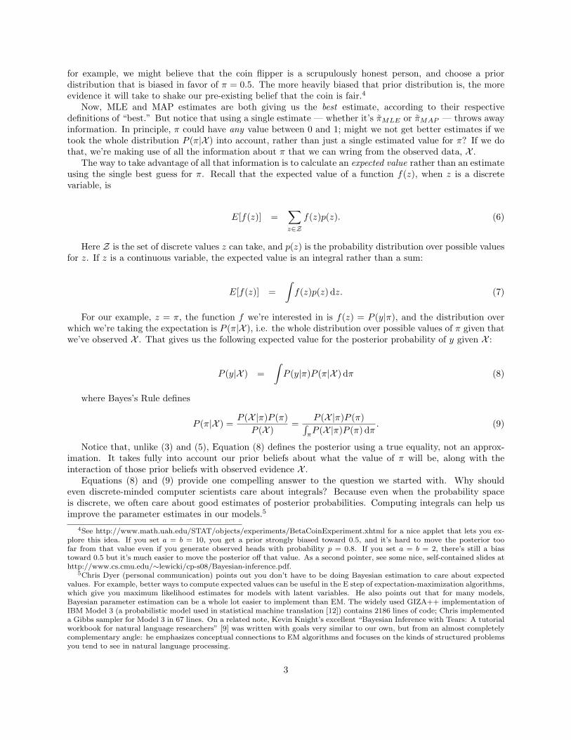
Figure 1: Probability of generating the coin-flip sequence HHHHTTTTTT, using different values forP (heads) on the x-axis. The value that maximizes the probability of the observed sequence, 0.4, is themaximum likelihood estimate (MLE).

count(H)count(H) + count(T)

=410

= 0.4 (1)

Formally, MLE produces the choice most likely to have generated the observed data.In this case, the most natural model µ has just a single parameter, π, namely the probability of heads

(see Figure 1).2 Letting X = HHHHTTTTTT represent the observed data, and y the outcome of the nextcoin flip, we estimate

πMLE = argmaxπ

P (X|π) (2)

P (y|X ) ≈ P (y|πMLE) (3)

On the other hand, sometimes we estimate probabilities using maximum a posteriori (MAP) estimation.A MAP estimate is the choice that is most likely given the observed data. In this case,

πMAP = argmaxπ

P (π|X )

= argmaxπ

P (X|π)P (π)P (X )

= argmaxπ

P (X|π)P (π) (4)

P (y|X ) ≈ P (y|πMAP ) (5)

In contrast to MLE, MAP estimation applies Bayes’s Rule, so that our estimate (4) can take into accountprior knowledge about what we expect π to be in the form of a prior probability distribution P (π).3 So,

2Specifically, µ models each choice as a Bernoulli trial, and the probability of generating exactly this heads-tails sequence fora given π is π4(1−π)6. If you type Plot[p^4(1-p)^6,{p,0,1}] into Wolfram Alpha, you get Figure 1, and you can immediatelysee that the curve tops out, i.e. the probability of generating the sequence is highest, exactly when p = 0.4. Confirm this byentering derivative of p^4(1-p)^6 and you’ll get 2

5= 0.4 as the maximum. Thanks to Kevin Knight for pointing out how

easy all this is using Wolfram Alpha. Also see discussion in Heinrich [7], Section 2.1.3We got to (4) from the desired posterior probability by applying Bayes’s Rule and then ignoring the denominator since the

argmax doesn’t depend on it.

2

for example, we might believe that the coin flipper is a scrupulously honest person, and choose a priordistribution that is biased in favor of π = 0.5. The more heavily biased that prior distribution is, the moreevidence it will take to shake our pre-existing belief that the coin is fair.4

Now, MLE and MAP estimates are both giving us the best estimate, according to their respectivedefinitions of “best.” But notice that using a single estimate — whether it’s πMLE or πMAP — throws awayinformation. In principle, π could have any value between 0 and 1; might we not get better estimates if wetook the whole distribution P (π|X ) into account, rather than just a single estimated value for π? If we dothat, we’re making use of all the information about π that we can wring from the observed data, X .

The way to take advantage of all that information is to calculate an expected value rather than an estimateusing the single best guess for π. Recall that the expected value of a function f(z), when z is a discretevariable, is

E[f(z)] =∑z∈Z

f(z)p(z). (6)

Here Z is the set of discrete values z can take, and p(z) is the probability distribution over possible valuesfor z. If z is a continuous variable, the expected value is an integral rather than a sum:

E[f(z)] =∫f(z)p(z) dz. (7)

For our example, z = π, the function f we’re interested in is f(z) = P (y|π), and the distribution overwhich we’re taking the expectation is P (π|X ), i.e. the whole distribution over possible values of π given thatwe’ve observed X . That gives us the following expected value for the posterior probability of y given X :

P (y|X ) =∫P (y|π)P (π|X ) dπ (8)

where Bayes’s Rule defines

P (π|X ) =P (X|π)P (π)

P (X )=

P (X|π)P (π)∫πP (X|π)P (π) dπ

. (9)

Notice that, unlike (3) and (5), Equation (8) defines the posterior using a true equality, not an approx-imation. It takes fully into account our prior beliefs about what the value of π will be, along with theinteraction of those prior beliefs with observed evidence X .

Equations (8) and (9) provide one compelling answer to the question we started with. Why shouldeven discrete-minded computer scientists care about integrals? Because even when the probability spaceis discrete, we often care about good estimates of posterior probabilities. Computing integrals can help usimprove the parameter estimates in our models.5

4See http://www.math.uah.edu/STAT/objects/experiments/BetaCoinExperiment.xhtml for a nice applet that lets you ex-plore this idea. If you set a = b = 10, you get a prior strongly biased toward 0.5, and it’s hard to move the posterior toofar from that value even if you generate observed heads with probability p = 0.8. If you set a = b = 2, there’s still a biastoward 0.5 but it’s much easier to move the posterior off that value. As a second pointer, see some nice, self-contained slides athttp://www.cs.cmu.edu/∼lewicki/cp-s08/Bayesian-inference.pdf.

5Chris Dyer (personal communication) points out you don’t have to be doing Bayesian estimation to care about expectedvalues. For example, better ways to compute expected values can be useful in the E step of expectation-maximization algorithms,which give you maximum likelihood estimates for models with latent variables. He also points out that for many models,Bayesian parameter estimation can be a whole lot easier to implement than EM. The widely used GIZA++ implementation ofIBM Model 3 (a probabilistic model used in statistical machine translation [12]) contains 2186 lines of code; Chris implementeda Gibbs sampler for Model 3 in 67 lines. On a related note, Kevin Knight’s excellent “Bayesian Inference with Tears: A tutorialworkbook for natural language researchers” [9] was written with goals very similar to our own, but from an almost completelycomplementary angle: he emphasizes conceptual connections to EM algorithms and focuses on the kinds of structured problemsyou tend to see in natural language processing.

3

1.2 Why sampling?

The trouble with integrals, of course, is that they can be very difficult to calculate. The methods we learnedin calculus class are fine for classroom exercises, but often cannot be applied to interesting problems in thereal world. Indeed, analytical solutions to (8) and the denominator of (9) might be impossible to obtain, sowe might not be able to determine the exact form of P (π|X ). Gibbs sampling allows us to sample from adistribution that asymptotically follows P (π|X ) without having to explicitly calculate the integrals.

1.2.1 Monte Carlo: a circle, a square, and a bag of rice

Gibbs Sampling is an instance of a Markov Chain Monte Carlo technique. Let’s start with the “MonteCarlo” part. You can think of Monte Carlo methods as algorithms that help you obtain a desired value byperforming simulations involving probabilistic choices. As a simple example, here’s a cute, low-tech MonteCarlo technique for estimating the value of π (the ratio of a circle’s circumference to its diameter).6

Draw a perfect square on the ground. Inscribe a circle in it — i.e. the circle and the square are centeredin exactly the same place, and the circle’s diameter has length identical to the side of the square. Now takea bag of rice, and scatter the grains uniformly at random inside the square. Finally, count the total numberof grains of rice inside the circle (call that C), and inside the square (call that S).

You scattered rice at random. Assuming you managed to do this pretty uniformly, the ratio between thecircle’s grains and the square’s grains (which include the circle’s) should approximate the ratio between thearea of the circle and the area of the square, so

C

S≈π(d2 )2

d2. (10)

Solving for π, we get π ≈ 4CS .

You may not have realized it, but we just solved a problem by approximating the values of integrals. Thetrue area of the circle, π(d2 )2, is the result of summing up an infinite number of infinitessimally small points;similarly for the the true area d2 of the square. The more grains of rice we use, the better our approximationwill be.

1.2.2 Markov Chains: walking the right walk

In the circle-and-square example, we saw the value of sampling involving a uniform distribution, since thegrains of rice were distributed uniformly within the square. Returning to the problem of computing expectedvalues, recall that we’re interested in Ep(x)[f(x)] (equation 7), where we’ll assume that the distribution p(x)is not uniform and, in fact, not easy to work with analytically.

Figure 2 provides an example f(z) and p(z) for illustration. Conceptually, the integral in equation (7)sums up f(z)p(z) over infinitely many values of z. But rather than touching each point in the sum exactlyonce, here’s another way to think about it: if you sample N points z(0), z(1), z(2), . . . , z(N) at random fromthe probability density p(z), then

Ep(z)[f(z)] = limN→∞

1N

N∑t=1

f(z(t)). (11)

That looks a lot like a kind of averaged value for f , which makes a lot of sense since in the discrete case(equation 6) the expected value is nothing but a weighted average, where the weight for each value of z isits probability.

Notice, though, that the value in the sum is just f(z(t)), not f(z(t))p(z(t)) as in the integral in equation (7).Where did the p(z) part go? Intuitively, if we’re sampling according to p(z), and count(z) is the number of

6We’re elaborating on the introductory example at http://en.wikipedia.org/wiki/Monte Carlo method.

4

p(z)

z1 z2 z3 z4

f(z)

Z

Figure 2: Example of computing expectation Ep(z)[f(z)]. (This figure was adapted from page 7 of thehandouts for Chris Bishop’s presentation “NATO ASI: Learning Theory and Practice”, Leuven, July 2002,http://research.microsoft.com/en-us/um/people/cmbishop/downloads/bishop-nato-2.pdf )

times we observe z in the sample, then 1N count(z) approaches p(z) as N →∞. So the p(z) is implicit in the

way the samples are drawn.7

Looking at equation (11), it’s clear that we can get an approximate value by sampling only a finite numberof times, T :

Ep(z)[f(z)] ≈ 1T

T∑t=1

f(z(t)). (12)

Progress! Now we have a way to approximate the integral. The remaining problem is this: how do wesample z(0), z(1), z(2), . . . , z(T ) according to p(z)?

There are a whole variety of ways to go about this; e.g., see Bishop [2] Chapter 11 for discussion of rejec-tion sampling, adaptive rejection sampling, adaptive rejection Metropolis sampling, importance sampling,sampling-importance-sampling,... For our purposes, though, the key idea is to think of z’s as points in astate space, and find ways to “walk around” the space — going from z(0) to z(1) to z(2) and so forth — sothat the likelihood of visiting any point z is proportional to p(z). Figure 2 illustrates the reasoning visually:walking around values for Z, we want to spend our time adding values f(z) to the sum when p(z) is large,e.g. devoting more attention to the space between z1 and z2, as opposed to spending time in less probableportions of the space like the part between z2 and z3.

A walk of this kind can be characterized abstractly as follows:

1: z(0) := a random initial point2: for t = 1 to T do3: z(t+1) := g(z(t))4: end for

7Okay — we’re playing a little fast and loose here by talking about counts: with Z continuous, we’re not going to see twoidentical samples z(i) = z(j), so it doesn’t really make sense to talk about counting how many times a value was seen. But wedid say “intuitively”, right?

5

Here g is a function that makes a probabilistic choice about what state to go to next according to anexplicit or implicit transition probability Ptrans(z(t+1)|z(0), z(1), . . . , z(t)).8

The part about probabilistic choices makes this a Monte Carlo technique. What will make it a MarkovChain Monte Carlo technique is defining things so that the next state you visit, z(t+1), depends only on thecurrent state z(t). That is,

Ptrans(z(t+1)|z(0), z(1), . . . , z(t)) = Ptrans(z(t+1)|z(t)). (13)

For you language folks, this is precisely the same idea as modeling word sequences using a bigram model,where here we have states z instead of having words w.

We included the subscript trans in our notation, so that Ptrans can be read as “transition probability”,in order to emphasize that these are state-to-state transition probabilities in a (first-order) Markov model.The heart of Markov Chain Monte Carlo methods is designing g so that the probability of visiting a state zwill turn out to be p(z), as desired. This can be accomplished by guaranteeing that the chain, as defined bythe transition probabilities Ptrans, meets certain conditions. Gibbs sampling is one algorithm that meetsthose conditions.9

1.2.3 The Gibbs sampling algorithm

Gibbs sampling is applicable in situations where Z has at least two dimensions, i.e. each point z is reallyz = 〈z1, . . . , zk〉, with k > 1. The basic idea in Gibbs sampling is that, rather than probabilistically pickingthe next state all at once, you make a separate probabilistic choice for each of the k dimensions, where eachchoice depends on the other k − 1 dimensions.10 That is, the probabilistic walk through the space proceedsas follows:

1: z(0) := 〈z(0)1 , . . . , z

(0)k 〉

2: for t = 1 to T do3: for i = 1 to k do4: z

(t+1)i ∼ P (Zi|z(t+1)

1 , . . . , z(t+1)i−1 , z

(t)i+1, . . . , z

(t)k )

5: end for6: end for

Note that we can obtain the distribution we are sampling from by using the definition of conditionalprobability:

P (Zi|z(t+1)1 , . . . , z

(t+1)i−1 , z

(t)i+1, . . . , z

(t)k ) =

P (z(t+1)1 , . . . , z

(t+1)i−1 , z

(t)i , z

(t)i+1, . . . , z

(t)k )

P (z(t+1)1 , . . . , z

(t+1)i−1 , z

(t)i+1, . . . , z

(t)k )

. (14)

Notice that the only difference between the numerator and the denominator is that the numerator is the fulljoint probability, including z(t)

i , whereas z(t)i is missing in the denominator. This will be important later.

One full execution of the inner loop and you’ve just computed your new point z(t+1) = g(z(t)) =〈z(t+1)

1 , . . . , z(t+1)k 〉.

You can think of each dimension zi as corresponding to a parameter or variable in your model. Usingequation (14), we sample the new value for each variable according to its distribution based on the valuesof all the other variables. During this process, new values for the variables are used as soon as you obtainthem. For the case of three variables:

• The new value of z1 is sampled conditioning on the old values of z2 and z3.8We’re deliberately staying at a high level here. In the bigger picture, g might consider and reject one or more states before

finally deciding to accept one and return it as the value for z(t+1). See discussions of the Metropolis-Hastings algorithm, e.g.Bishop [2], Section 11.2.

9We told you we were going to keep theory to a minimum, didn’t we?10There are, of course, variations on this basic scheme. For example, “blocked sampling” groups the variables into b < k

blocks and the variables in each block are sampled together based on the other b− 1 blocks.

6

• The new value of z2 is sampled conditioning on the new value of z1 and the old value of z3.

• The new value of z3 is sampled conditioning on the new values of z1 and z2.

1.3 The remainder of this document

So, there you have it. Gibbs sampling makes it possible to obtain samples from probability distributionswithout having to explicitly calculate the values for their marginalizing integrals, e.g. computing expectedvalues, by defining a conceptually straightforward approximation. This approximation is based on the ideaof a probabilistic walk through a state space whose dimensions correspond to the variables or parameters inyour model.

Trouble is, from what we can tell, most descriptions of Gibbs sampling pretty much stop there (if they’veeven gone into that much detail). To someone relatively new to this territory, though, that’s not nearly farenough to figure out how to do Gibbs sampling. How exactly do you implement the “sampling from thefollowing distribution” part at the heart of the algorithm (equation 14) for your particular model? How doyou deal with continuous parameters in your model? How do you actually generate the expected values you’reultimately interested in (e.g. equation 8), as opposed to just doing the probabilistic walk for T iterations?

Just as the first part of this document aimed at explaining why, the remainder aims to explain how.In Section 2, we take a very simple probabilistic model — Naıve Bayes — and describe in considerable(painful?) detail how to construct a Gibbs sampler for it. This includes two crucial things, namely how toemploy conjugate priors and how to actually sample from conditional distributions per equation (14).

In Section 3 we discuss how to actually obtain values from a Gibbs sampler, as opposed to merely watchingit walk around the state space. (Which might be entertaining, but wasn’t really the point.) Our discussionincludes convergence and burn-in, auto-correlation and lag, and other practical issues.

In Section 4 we conclude with pointers to other things you might find it useful to read, as well as aninvitation to tell us how we could make this document more accurate or more useful.

2 Deriving a Gibbs Sampler for a Naıve Bayes Model

In this section we consider Naive Bayes models.11 Let’s assume that items of interest are documents, thatthe features under consideration are the words in the document, and that the document-level class variablewe’re trying to predict is a sentiment label whose value is either 0 or 1. For ease of reference, we presentour notation in Figure 3. Figure 4 describes the model as a “plate diagram”, to which we will refer whendescribing the model.

2.1 Modeling How Documents are Generated

We represent each document as a bag of words. Given an unlabeled document Wj , our goal is to pickthe best label Lj = 0 or Lj = 1. Sometimes we will refer to 0 and 1 as classes instead of labels. Infurther discussion it will be convenient for us to refer to the sets of documents sharing the same label, so fornotational convenience we define the sets C0 = {Wj |Lj = 0} and C1 = {Wj |Lj = 1}. The usual treatmentof these models is to equate “best” with “most probable”, and therefore our goal is to choose the label Ljfor Wj that maximizes P (Lj |Wj). Applying Bayes’s Rule,

Lj = argmaxL

P (L|Wj) = argmaxL

P (Wj |L)P (L)P (Wj)

= argmaxL

P (Wj |L)P (L),

where the denominator P (Wj) is omitted because it does not depend on L.This application of Bayes’s rule (the “Bayes” part of “Naıve Bayes”) allows us to think of the model in

terms of a “generative story” that accounts for how documents are created. According to that story, we11We assume the reader is familiar with Naive Bayes. For a refresher, see [14].

7

V number of words in the vocabulary.N number of documents in the corpus.γπ1, γπ0 hyperparameters of the Beta distribution.γθ hyperparameter vector for the multinomial prior.γθi pseudocount for word i.Cx set of documents labeled x.C the set of all documents.C0 (C1) number of documents labeled 0 (1).Wj document j’s frequency distribution.Wji frequency of word i in document j.L vector of document labels.Lj label for document j.Rj number of words in document j.θi probability of word i.θx,i probability of word i from the distribution of class x.NCx(i) number of times word i occurs in the set of all documents labeled x.C(−j) set of all documents except Wj

L(−j) vector of all document labels except LjC

(−j)0 (C(−j)

1 ) number of documents labeled 0 (1) except for Wj

µ set of hyperparameters 〈γπ1, γπ0,γθ〉

Figure 3: Notation.

2

Nγπ Lj

RjWjk

γθ

π

θ

Figure 4: Naive Bayes plate diagram

8

first pick the class label of the document, Lj ; our model will assume that’s done by flipping a coin whoseprobability of heads is some value π = P (Lj = 1). We can express this a little more formally as

Lj ∼ Bernoulli(π).

Then, for every one of the Rj word positions in the document, we pick a word wi independently bysampling randomly according to a probability distribution over words. Which probability distribution weuse is based on the label Lj of the document, so we’ll write them as θ0 and θ1. Formally one would describethe creation of document j’s bag of words as

Wj ∼ Multinomial(Rj ,θ). (15)

The assumption that the words are chosen independently is the reason we call the model “naıve”.Notice that logically speaking, it made sense to describe the model in terms of two separate probability

distributions, θ0 and θ1, each one being a simple unigram distribution. The notation in (15) doesn’t explicitlyshow that what happens in generating Wj depends on whether Lj was 0 or 1. Unfortunately, that notationalchoice seems to be standard, even though it’s less transparent.12 We indicate the existence of two θs byincluding the 2 in the lower rectangle of Figure 4, but many plate diagrams in the literature would not.Another, perhaps clearer way to describe the process would be

Wj ∼ Multinomial(Rj ,θLj ). (16)

And that’s it: our “generative story” for the creation of a whole set of labeled documents 〈Wn,Ln〉,according to the Naıve Bayes model, is that this simple document-level generative story gets repeated Ntimes, as indicated by the N in the upper rectangle in Figure 4.

2.2 Priors

Well, ok, that’s not completely it. Where did π come from? Our generative story is going to assume thatbefore this whole process began, we also picked π randomly. Specifically we’ll assume that π is sampled froma Beta distribution with parameters γπ1 and γπ0. These are referred to as hyperparameters because they areparameters of a prior, which is itself used to pick parameters of the model. In Figure 4 we represent these twohyperparameters as a single two-dimensional vector γπ = 〈γπ1, γπ0〉. When γπ1 = γπ0 = 1, Beta(γπ1, γπ0)is just a uniform distribution, which means that any value for π is equally likely. For this reason we callBeta(1, 1) an “uninformed prior”.

Similarly, where do θ0 and θ1 come from? Just as the Beta distribution can provide an uninformed priorfor a distribution making a two-way choice, the Dirichlet distribution can provide an uninformed prior forV -way choices, where V is the number of words in the vocabulary. Let γθ be a V -dimensional vector wherethe value of every dimension equals 1. If θ0 is sampled from Dirichlet(γθ), every probability distributionover words will be equally likely. Similarly, we’ll assume θ1 is sampled from Dirichlet(γθ).13 Formally

π ∼ Beta(γπ)

θ ∼ Dirichlet(γθ)

Choosing the Beta and Dirichlet distributions as priors for binomial and multinomial distributions, re-spectively, helps the math work out cleanly. We’ll discuss this in more detail in Section 2.4.2.

12The actual basis for removing the subscripts on the parameters θ is that we assume the data from one class is independentof the parameter estimation of all the other classes, so essentially when we derive the probability expressions for one class theothers look the same [19].

13Note that θ0 and θ1 are sampled separately. There’s no assumption that they are related to each other at all. Also, it’sworth noting that a Dirichlet distribution is a Beta distribution if the dimension V = 2. Dirichlet generalizes Beta in the sameway that multinomial generalizes binomial. Now you see why we took the trouble to represent γπ1 and γπ0 as a 2-dimensionalvector γπ .

9

2.3 State space and initialization

Following Pedersen [17, 18], we’re going to describe the Gibbs sampler in a completely unsupervised settingwhere no labels at all are provided as training data. We’ll then briefly explain how to take advantage oflabeled data.

State space. Recall that the job of a Gibbs sampler is to walk through an k-dimensional state space definedby the random variables 〈Z1, Z2, . . . Zk〉 in the model. Every point in that walk is a collection 〈z1, z2, . . . zk〉of values for those variables.

In the Naıve Bayes model we’ve just described, here are the variables that define the state space.

• one scalar-valued variable π

• two vector-valued variables, θ0 and θ1

• binary label variables L, one for each of the N documents

We also have one vector variable Wj for each of the N documents, but these are observed variables, i.e.their values are already known (and which is why Wjk is shaded in Figure 4).

Initialization. The initialization of our sampler is going to be very easy. Pick a value π by sampling fromthe Beta(γπ1, γπ0) distribution. Then, for each j, flip a coin with success probability π, and assign label L(0)

j

— that is, the label of document j at the 0th iteration – based on the outcome of the coin flip. Similarly,you also need to initialize θ0 and θ1 by sampling from Dirichlet(γθ).

2.4 Deriving the Joint Distribution

Recall that for each iteration t = 1 . . . T of sampling, we update every variable defining the state space bysampling from its conditional distribution given the other variables, as described in equation (14).

Here’s how we’re going to proceed:

• We will define the joint distribution of all the variables, corresponding to the numerator in (14).

• We simplify our expression for the joint distribution.

• We use our final expression of the joint distribution to define how to sample from the conditionaldistribution in (14).

• We give the final form of the sampler as pseudocode.

2.4.1 Expressing and simplifying the joint distribution

According to our model, the joint distribution for the entire document collection is P (C,L, π,θ0,θ1; γπ1, γπ0,γθ).The semicolon indicates that the values to its right are parameters for this joint distribution. Another wayto say this is that the variables to the left of the semicolon are conditioned on the hyperparameters given tothe right of the semicolon. Using the model’s generative story, and, crucially, the independence assumptionsthat are a part of that story, the joint distribution can decomposed into a product of several factors:14

P (π|γπ1, γπ0)P (L|π)P (θ0|γθ)P (θ1|γθ)P (C0|θ0,L)P (C1|θ1,L)

Let’s look at each of these in turn.14Note that we can also obtain the products of the joint distribution directly from our graphical model, Figure 4 by multiplying

together each latent variable conditioned on its parents.

10

• P (π|γπ1, γπ0). The first factor is the probability of choosing this particular value of π given that γπ1

and γπ0 are being used as the hyperparameters of the Beta distribution. By definition of the Betadistribution, that probability is:

P (π|γπ1, γπ0) =Γ(γπ1 + γπ0)Γ(γπ1)Γ(γπ0)

πγπ1−1(1− π)γπ0−1 (17)

And because

Γ(γπ1 + γπ0)Γ(γπ1)Γ(γπ0)

is a constant that doesn’t depend on π, we can rewrite this as:

P (π|γπ1, γπ0) = c πγπ1−1(1− π)γπ0−1. (18)

The constant c is a normalizing constant that makes sure P (π|γπ1, γπ0) sums to 1 over all π. Γ(x)is the gamma function, a continuous-valued generalization of the factorial function. We could alsoexpress (18) as

P (π|γπ1, γπ0) ∝ πγπ1−1(1− π)γπ0−1. (19)

• P (L|π). The second factor is the probability of obtaining this specific sequence L of N binary labels,given that the probability of choosing label = 1 is π. That’s

P (L|π) =N∏n=1

πLn(1− π)(1−Ln) (20)

= πC1(1− π)C0 (21)

Recall from Figure 3 that C0 and C1 are nothing more than the number of documents labeled 1 and0 respectively.15

• P (θ0|γθ) and P (θ1|γθ). The third factors are the probability of having sampled these particular choicesof word distributions, given that γθ was used as the hyperparameter of the Dirichlet distribution.

Since the θ distributions are independent of each other, let’s make the notation a bit easier to read hereand consider each of them in isolation, allowing us to momentarily elide the subscript saying which oneis which. By the definition of the Dirichlet distribution, the probability of each word distribution is

P (θ|γθ) =Γ(∑Vi=1γθi)∏V

i=1 Γ(γθi)

V∏i=1

θγθi−1i (22)

= c′V∏i=1

θγθi−1i (23)

∝V∏i=1

θγθi−1i (24)

Recall that γθi denotes the value of vector γθ’s ith dimension, and similarly, θi is the value for theith dimension of vector θ, i.e. the probability assigned by this distribution to the ith word in thevocabulary. c′ is another normalization constant that we can discard by changing the equality to aproportionality.

15Of course we can represent these quantities given the variables we already have, but we define these in the interests ofsimplifying the equations somewhat.

11

• P (C0|θ0,L) and P (C1|θ1,L). These are the probabilities of generating the contents of the bags ofwords in each of the two document classes.

Generating the bag of words Wn for document n depends on that document’s label, Ln and the wordprobability distribution associated with that label, θLn (so θLn is either θ0 or θ1). For notationalsimplicity, let’s let θ = θLn :

P (Wn|L,θLn) =V∏i=1

θWnii (25)

Here θi is the probability of word i in distribution θ, and the exponent Wni is the frequency of word iin Wn.

Now, since the documents are generated independently of each other, we can multiply the value in (25)for each of the documents in each class to get the combined probability of all the observed bags ofwords within a class:

P (Cx|L,θx) =∏n∈Cx

V∏i=1

θWnix,i (26)

=V∏i=1

θNCx (i)x,i (27)

Where NCx(i) gives the count of word i in documents with class label x.

2.4.2 Choice of Priors and Simplifying the Joint Probability Expression

So why did we pick the Dirichlet distribution as our prior for θ0 and θ1 and the Beta distribution as ourprior for π? Let’s look at what happens in the process of simplifying the joint distribution and see whathappens to our estimates of θ (where this can be either θ0 or θ1) and π once we observe some evidence (i.e.the words from a single document). Using (19) and (21) from above:

P (π|L; γπ1, γπ0) = P (L|π)P (π|γπ1, γπ0) (28)∝

[πC1(1− π)C0

] [πγπ1−1(1− π)γπ0−1

](29)

∝ πC1+γπ1−1(1− π)C0+γπ0−1 (30)

Likewise, for θ using (24) and (25) from above:

P (θ|Wn; γθ) = P (Wn|θ)P (θ|γθ)

∝V∏i=1

θWnii

V∏i=1

θγθi−1i

∝V∏i=1

θWni+γθi−1i (31)

If we use the words in all of the documents of a given class, then we have:

P (θx|Cx; γθ) ∝V∏i=1

θNCx (i)+γθi−1x,i (32)

12

Notice that (30) is an unnormalized Beta distribution, with parameters C1 + γπ1 and C0 + γπ0, and (32)is an unnormalized Dirichlet distribution, with parameter vector 〈NCx(i) + γθi〉 for 1 ≤ i ≤ V . When theposterior probability distribution is of the same family as the likelihood probability distribution — that is, thesame functional form, just with different arguments — it is said to be the conjugate prior of the posterior.The Beta distribution is the conjugate prior for binomial (and Bernoulli) distributions and the Dirichletdistribution is the conjugate prior for multinomial distributions. Also notice what role the hyperparametersplayed—they are added just like observed evidence. It is for this reason that the hyperparameters aresometimes referred to as pseudocounts.

Okay, so if we multiply together the individual factors from Section 2.4.1 as simplified above (in Section2.4.2) and let µ = 〈γπ1, γπ0,γθ〉 we can express the full joint distribution as:

P (C,L, π,θ0,θ1; µ) ∝ πC1+γπ1−1(1− π)C0+γπ0−1V∏i=1

θNC0 (i)+γθi−1

0,i θNC1 (i)+γθi−1

1,i (33)

2.4.3 Integrating out π

Having illustrated how to derive the joint distribution for a model, as in (33), it turns out that, for thisparticular model, we can make our lives a little bit simpler: we can reduce the effective number of parametersin the model by integrating our joint distribution with respect to π. This has the effect of taking all possiblevalues of π into account in our sampler, without representing it as a variable explicitly and having to sampleit at every iteration. Intuitively, “integrating out” a variable is an application of precisely the same principleas computing the marginal probability for a discrete distribution. For example, if we have an expression forP (a, b, c), we can compute P (a, b) by summing over all possible values of c, i.e. P (a, b) =

∑c P (a, b, c). As

a result, c is “there” conceptually, in terms of our understanding of the model, but we don’t need to dealwith manipulating it explicitly as a parameter. With a continuous variable, the principle is the same, butwe integrate over all possible values of the variable rather than summing.

So, we have

P (L,C,θ0,θ1; µ) =∫π

P (L,C,θ0,θ1, π; µ) dπ (34)

=∫π

P (π|γπ1, γπ0)P (L|π)P (θ0|γθ)P (θ1|γθ)P (C0|θ0,L)P (C1|θ1,L) dπ (35)

= P (θ0|γθ)P (θ1|γθ)P (C0|θ0,L)P (C1|θ1,L)∫π

P (π|γπ1, γπ0)P (L|π) dπ (36)

At this point let’s focus our attention on the integrand only and substitute the true distributions from(17) and (21).

∫π

P (π|γπ1, γπ0)P (L|π) dπ =∫π

Γ(γπ1 + γπ0)Γ(γπ1)Γ(γπ0)

πγπ1−1(1− π)γπ0−1πC1(1− π)C0 dπ (37)

=Γ(γπ1 + γπ0)Γ(γπ1)Γ(γπ0)

∫π

πC1+γπ1−1(1− π)C0+γπ0−1 dπ (38)

Here’s where our use of conjugate priors pays off. Notice that the integrand in (38) is a Beta distribution withparameters C1 +γπ1 and C0 +γπ0. This means that the value of the integral is just the normalizing constantfor that distribution, which is easy to look up (e.g. in the entry for the Beta distribution in Wikipedia): thenormalizing constant for distribution Beta(C1 + γπ1, C0 + γπ0) is

Γ(C1 + γπ1)Γ(C0 + γπ0)Γ(C0 + C1 + γπ1 + γπ0)

13

Making that substitution in (38), and also substituting N = C0 + C1, we arrive at∫π

P (π|γπ1, γπ0)P (L|π) dπ =Γ(γπ1 + γπ0)Γ(γπ1)Γ(γπ0)

Γ(C1 + γπ1)Γ(C0 + γπ0)Γ(N + γπ1 + γπ0)

(39)

Substituting (39) and the definitions of the probability distributions from Section 2.4.1 back into (36)gives us

P (L,C,θ0,θ1; µ) ∝ Γ(γπ1 + γπ0)Γ(γπ1)Γ(γπ0)

Γ(C1 + γπ1)Γ(C0 + γπ0)Γ(N + γπ1 + γπ0)

V∏i=1

θNC0 (i)+γθi−1

0,i θNC1 (i)+γθi−1

1,i (40)

Okay, so it would be reasonable at this point to ask, “I thought the point of integrating out π was tosimplify things, so why did we just ’simplify’ the joint expression by adding in a bunch of these Gammafunctions everywhere?” Good question–hold that thought until we derive the sampler.

2.5 Building the Gibbs Sampler

The definition of a Gibbs sampler specifies that in each iteration we assign a new value to variable Zi bysampling from the conditional distribution

P (Zi|z(t+1)1 , . . . , z

(t+1)i−1 , z

(t)i+1, . . . , z

(t)r ).

So, for example, to assign the value of L(t+1)1 , we need to compute this conditional distribution:16

P (L1|L(t)2 , . . . ,L(t)

N ,C,θ(t)0 ,θ

(t)1 ; µ),

To assign the value of L(t+1)2 , we need to compute

P (L2|L(t+1)1 ,L(t)

3 , . . . ,L(t)N ,C,θ(t)

0 ,θ(t)1 ; µ),

and so forth for L(t+1)3 through L(t+1)

N . To assign the value of θ0 we need to computeSimilarly, to assign the value of θ0 we need to sample from the conditional distribution

P (θ(t+1)0 |L(t+1)

1 ,L(t+1)2 , . . . ,L(t+1)

N ,C,θ(t)1 ; µ),

and, for θ1,

P (θ(t+1)1 |L(t+1)

1 ,L(t+1)2 , . . . ,L(t+1)

N ,C,θ(t+1)0 ; µ),

Intuitively, at the start of an iteration t, we have a collection of all our current information at thispoint in the sampling process. That information includes the word count for each document, the number ofdocuments labeled 0, the number of documents labeled 1, the word counts for all documents labeled 0, theword counts for all documents labeled 1, the current label for each document, the current values of θ0 and θ1,etc. When we want to sample the new label for document j, we temporarily remove all information (i.e. wordcounts and label information) about this document from that collection of information. Then we look at theconditional probability that Lj = 0 given all the remaining information, and the conditional probability thatLj = 1 given the same information, and we sample the new label L(t+1)

j by choosing randomly according to

the relative weight of those two conditional probabilities. Sampling to get the new values θ(t+1)0 and θ

(t+1)1

operates according to the same principal.16There’s no superscript on the bags of words C because they’re fully observed and don’t change from iteration to iteration.

14

2.5.1 Sampling for Document Labels

Okay, so how do we actually do the sampling? We’re almost there. As the final step in our journey, we showhow to select all of the new document labels Lj and the new distributions θ0 and θ1 during each iterationof the sampler. By definition of conditional probability,

P (Lj |L(−j),C(−j),θ0,θ1; µ) =P (Lj ,Wj ,L(−j),C(−j),θ0,θ1; µ)

P (L(−j),C(−j),θ0,θ1; µ)(41)

=P (L,C,θ0,θ1; µ)

P (L(−j),C(−j),θ0,θ1; µ)(42)

where L(−j) are all the document labels except Lj , and C(−j) is the set of all documents except Wj . Thedistribution is over two possible outcomes, Lj = 0 and Lj = 1.

Notice that the numerator is just the complete joint probability described in (40). In the denominator,we have the same expression, minus all the information about document Wj . Therefore we can work outwhat (42) should look like by considering the three factors in (40), one at a time. For each factor, we willremind ourselves of what it looks like in the numerator (which includes Wj), and work out what it shouldlook like in the denominator (excluding Wj), for each of the two outcomes.

The first factor in (40),

Γ(γπ1 + γπ0)Γ(γπ1)Γ(γπ0)

, (43)

is very easy. It depends only on the hyperparameters, so removing information about Wj has no impacton its value. Since it will be the same in both the numerator and denominator of (42), it will cancel out.Excellent! Two factors to go.

Let’s look at the second factor of (40). Taking all documents into account including Wj , this is

Γ(C1 + γπ1)Γ(C0 + γπ0)Γ(N + γπ1 + γπ0)

. (44)

Now, in order to compute the denominator of (42), we remove document Wj from consideration. How doesthat change things? It depends on what Lj was during the previous iteration. Whether Lj = 0 or Lj = 1during the previous iteration, the corpus size is effectively reduced from N to N − 1, and the size of one ofthe document classes is smaller by one compared to its value in the numerator. If Lj = 0 when we removeit, then we will have C(−j)

0 = C0 − 1 and C(−j)1 = C1. If Lj = 1 during the previous iteration, then we will

have C0 = C(−j)0 and C

(−j)1 = C1 − 1. In each case, removing Wj only changes the information we know

about one class, which means that of the two terms in the numerator of this factor, one of them is going tobe the same in the numerator and the denominator of (42). That’s going to cause the terms from one of theclasses (the one Wj did not belong to after the previous iteration) to cancel out.

Let x ∈ {0, 1} be the outcome we’re considering, i.e. the one for which C(−j)x = Cx − 1.17 If we use x

and reorganize the expression a bit, the second factor of (42) can be rewritten from

Γ(C1+γπ1)Γ(C0+γπ0)Γ(N+γπ1+γπ0)

Γ(C(−j)0 +γπ0)Γ(C

(−j)1 +γπ1)

Γ(N+γπ1+γπ0−1)

to

Γ(Cx + γπx)Γ(N + γπ1 + γπ0 − 1)Γ(N + γπ1 + γπ0)Γ(Cx + γπx − 1)

(45)

17Crucially, note that x here is not L(t)j , the label of document j at the previous iteration. We are pulling document j out

of the collection, effectively obviating our knowledge of its current label, and then constructing a distribution over the twopossibilities, Lj = 0 and Lj = 1. So we need for our expression to take x as a parameter, allowing us to build a probabilitydistribution by asking “what if x = 0?” and “what if x = 1?”.

15

Using the fact that Γ(a+ 1) = aΓ(a) for all a, we can simplify further to get

Cx + γπx − 1N + γπ1 + γπ0 − 1

(46)

Look, no more pesky Gammas!Finally, the third factor in (40) is

V∏i=1

θNC0 (i)+γθi−1

0,i θNC1 (i)+γθi−1

1,i . (47)

When we look at what changes when we remove Wj from consideration, in order to write the correspondingexpression in the denominator of (42), we see that it will behave in the same way as the second factor. Oneof the classes remains unchanged, so one of the terms, either the θ0 or θ1, will cancel out when we do thedivision. If, similar to above, we let x be the class for which C

(−j)x = Cx − 1, then we can again capture

both cases in one expression:

V∏i=1

θNCx (i)+γθi−1x,i

θN

C(−j)x

(i)+γθi−1

x,i

=V∏i=1

θWji

x,i (48)

With that, we have finished working through the three factors in (40), which means we have worked outhow to express the numerator and denominator of (42), factor by factor. Recombining the factors, we getthe following expression for the conditional distribution in (42): for x ∈ {0, 1},

Pr(Lj = x|L(−j),C(−j),θ0,θ1; µ) =Cx + γπx − 1

N + γπ1 + γπ0 − 1

V∏i=1

θWji

x,i (49)

Let’s take a step back and take a look at what this equation is telling us about how a label is chosen. Itsfirst factor gives us an indication of how likely it is that Lj = x considering only the distribution of the otherlabels. So, for example, if the corpus had more class 0 documents than class 1 documents, this factor wouldtend to push the label toward class 0. Its second factor is like a word distribution “fitting room.” We get anindication of how well the words in Wj “fit” with each of the two distributions. If, for example, the wordsfrom Wj “fit” better with distribution θ0 (by having a larger value for the document probability using θ0)then this factor will push the label toward class 0 as well.

So (finally!) here’s the actual procedure to sample from the conditional distribution in (42):

1. Let value0 = expression (49) with x = 0

2. Let value1 = expression (49) with x = 1

3. Let the distribution be 〈 value0value0+value1 ,

value1value0+value1 〉

4. Select the value of L(t+1)j as the result of a Bernoulli trial (weighted coin flip) according to this distri-

bution.

2.5.2 Sampling for θ

We’ll follow a similar procedure to determine how to sample for new values of θ0 and θ1. Since the estimationof the two distributions is independent of one another, we’re going to omit the subscripts on θ to make thenotation a bit easier to digest. Just like above, we’ll need to derive an expression for the probability of θgiven all other variables, but our work is a bit simpler in this case. Observe,

P (θ|C,L; µ) ∝ P (C,L|θ)P (θ|µ) (50)

16

Furthermore, recall that, since we used conjugate priors, this posterior, like the prior, works out to be aDirichlet distribution. We actually derived the full expression in Section 2.4.2, but we don’t need the fullexpression here. All we need to do to sample a new distribution is to make another draw from a Dirichletdistribution, but this time with parameters NCx(i) + γθi for each i in V . For notational convenience, let’sdefine the V dimensional vector t such that each ti = NCx(i) + γθi, where x is again either 0 or 1 dependingon which θ we are resampling. We then sample a new θ as:

θ ∼ Dirichlet(t) (51)

How do you actually implement sampling from a new Dirichlet distribution? To sample a random vectora = 〈a1, . . . , aV 〉 from the V -dimensional Dirichlet distribution with parameters 〈α1, . . . , αV 〉, one fast wayis to draw V independent samples y1, . . . , yV from gamma distributions, each with density

Gamma(αi, 1) =yαi−1i e−yi

Γ(αi), (52)

and then set ai = yi/∑Vj=1 yj (i.e., just normalize each of the gamma distribution draws).18

2.5.3 Taking advantage of documents with labels

Using labeled documents is relatively painless: just don’t sample Lj for those documents! Always keepLj equal to the observed label. The documents will effectively serve as “ground truth” evidence for thedistributions that created them. Since we never sample for their labels, they will always contribute to thecounts in (49) and (51) and will never be subtracted out.

2.5.4 Putting it all together

Initialization. Define the priors as in Section 2.2 and initialize them as described in Section 2.3.

1: for t := 1 to T do2: for j := 1 to N do3: if j is not a training document then4: Subtract j’s word counts from the total word counts of whatever class it’s currently a member of5: Subtract 1 from the count of documents with label Lj6: Assign a new label L(t+1)

j to document j as described at the end of Section 2.5.1

7: Add 1 to the count of documents with label L(t+1)j

8: Add j’s word counts to the total word counts for class L(t+1)j

9: end if10: end for11: t0 := vector of total word counts from class 0, including pseudocounts12: θ0 ∼ Dirichlet(t0), as described in Section 2.5.213: t1 := vector of total word counts from class 1, including pseudocounts14: θ1 ∼ Dirichlet(t1), as described in Section 2.5.215: end for

Sampling iterations. Notice that as soon as a new label for Lj is assigned, this changes the counts thatwill affect the labeling of the subsequent documents. This is, in fact, the whole principle behind a Gibbssampler!

That concludes the discussion of how sampling is done. We’ll see how to get from the output of thesampler to estimated values for the variables in Section 3.

18For details, see http://en.wikipedia.org/wiki/Dirichlet distribution (version of April 12, 2010).

17

2.6 Optional: A Note on Integrating out Continuous Parameters

At this point you might be asking yourself why we were able to integrate out the continuous parameter πfrom our model, but did not do something similar with the two word distributions θ0 and θ1. The idea ofdoing this even looks promising, but there’s a subtle problem that will get us into trouble and end up leavingus with an expression filled with Γ functions that will not cancel out. Let us go through the derivations andsee where it leads us. If you follow this piece of the discussion, then you really understand the details!19

Our goal here would be to obtain the probability that a document was generated from the same dis-tribution that generated the words of a particular class of documents, Cx. We would then use this as areplacement for the product in (48). We start first by calculating the probability of making a single worddraw given the other words in the class, subtracting out the information about Wj . In the equations thatfollow there’s an implicit (−j) superscript on all of the counts. If we let wk denote the word at some positionk in Wj then,

Pr(wk = y|C(−j)x ; γθ) =

∫∆

Pr(wk = y|θ)P (θ|C(−j)x ; γθ)dθ (53)

=∫

∆

θx,yΓ(∑Vi=1NCx(i) + γθi)∏V

i=1 Γ(NCx(i) + γθi)

V∏i=1

θNCx (i)+γθi−1x,i dθ (54)

=Γ(∑Vi=1NCx(i) + γθi)∏V

i=1 Γ(NCx(i) + γθi)

∫∆

θx,y

V∏i=1

θNCx (i)+γθi−1x,i dθ (55)

=Γ(∑Vi=1NCx(i) + γθi)∏V

i=1 Γ(NCx(i) + γθi)

∫∆

θNCx (y)+γθyx,y

V∏i=1∧i6=y

θNCx (i)+γθi−1x,i dθ (56)

=Γ(∑Vi=1NCx(i) + γθi)∏V

i=1 Γ(NCx(i) + γθi)

Γ(NCx(y) + γθy + 1)∏Vi=1∧i 6=y Γ(NCx(i) + γθi)

Γ(1 +∑Vi=1NCx(i) + γθi)

(57)

=NCx(y) + γθy∑Vi=1NCx(i) + γθi

(58)

The process we use is actually the same as the process used to integrate π, just in the multidimensionalcase. The set ∆ is the probability simplex of θ, namely the set of all θ such that

∑i θi = 1. We get to (54)

by substitution from the formulas we derived in Section 2.4.2, then (55) by factoring out the normalizationconstant for the Dirichlet distribution, since it is constant with respect to θ. Note that the integrand of(56) is actually another Dirichlet distribution, so its integral is its normalization constant (same reasoningas before). We substitute this in to obtain (57). Using the property of Γ that Γ(x+ 1) = xΓ(x) for all x, wecan again cancel all of the Γ terms.

At this point, even though we have a simple and intuitive result for the probability of drawing a singleword from a Dirichlet, we actually need the probability of drawing all words in Wj from the Dirichletdistribution. What we’d really like to do is assume that the words within a particular document are drawnfrom the same distribution, and just calculate the probability of Wj by multiplying (58) over all words in thevocabulary. But we cannot do that, since, without the values of θ being known, we cannot make independentdraws from a Dirichlet distribution since our draws have an effect on what our estimate of θ is!

We can see this two different ways. First, instead of drawing one word in equation (53), do the derivationby drawing two words at a time.20 You’ll find that once you hit (57), you’ll have an extra set of Gammafunctions that won’t cancel out nicely. The second way to see it is actually by looking at the plate diagramfor the model, Figure 4. Each θ effectively has Rj arrows coming out of it for each document j to individual

19The authors thank Wu Ke, who really understood the details, for pointing out our error in an earlier version of this documentand providing the illustrating example we go through next.

20This is what Wu Ke did to demonstrate his point to us.

18

words, so every word within a document is in the Markov blanket 21 of the others; therefore we can’t assumethat the words are independent without a fixed θ. At issue here isn’t just that there are multiple instancesof words coming out of each theta, but crucially that those instances are sampled at the same time.

The lesson here is to be careful when you integrate out parameters. If you’re doing a single draw from amultinomial, then integrating out a continuous parameter can make the sampler simpler, since you won’t haveto sample for it at every iteration. If, on the other hand, you do multiple draws from the same multinomial,integration (although possible) will result in an expression that involves Gamma functions. CalculatingGamma functions is undesirable since they are computationally expensive, so they can slow down a samplersignificantly.

3 Producing values from the output of a Gibbs sampler

The initialization and sampling iterations in the Gibbs sampling algorithm will produce values for each ofthe variables, for iterations t = 1, 2, . . . , T . In theory, the approximated value for any variable Zi can simplybe obtained by calculating:

1T

T∑t=1

z(t)i , (59)

as discussed in equation (12). However, expression (59) is not always used directly. There are severaladditional details to note that are a part of typical sampling practice.22

Convergence and burn-in iterations. Depending on the values chosen during the initialization step,it may take some time for the Gibbs sampler to reach a point where the points 〈z(t)

1 , z(t)2 , . . . z

(t)r 〉 are all

coming from the stationary distribution of the Markov chain, which is an assumption of the approximationin (59). In order to avoid the estimates being contaminated by the values at iterations before that point,some practitioners generally discard the values at iterations t < B, which are referred to as the “burn-in”iterations, so that the average in (59) is taken only over iterations B + 1 through T .23

Autocorrelation and lag. The approximation in (59) assumes the samples for Zi are independent, butwe know they’re not, because they were produced by a process that conditions on the previous point in thechain to generate the next point. This is referred to as autocorrelation (sometimes serial autocorrelation),i.e. correlation between successive values in the data.24 In order to avoid autocorrelation problems (so thatthe chain “mixes well”), many implementations of Gibbs sampling average only every Lth value, where L isreferred to as the lag.25 In this context, Jordan Boyd-Graber (personal communication) also recommendslooking at Neal’s [15] discussion of likelihood as a metric of convergence.

21The Markov blanket of a node in a graphical model consists of that node’s parents, its children, and the coparents of itschildren. [16].

22Jason Eisner (personal communication) argues, with some support from the literature, that burn-in, lag, and multiplechains are in fact unnecessary and it is perfectly correct to do a single long sampling run and keep all samples. See [4, 5],MacKay ([13], end of section 29.9, page 381) and Koller and Friedman ([10], end of section 12.3.5.2, page 522).

23As far as we can tell, there is no principled way to choose the “right” value for B in advance. There are a variety ofways to test for convergence, and to measure autocorrelation; see, e.g., Brian J. Smith, “boa: An R Package for MCMCOutput Convergence Assessment and Posterior Inference”, Journal of Statistical Software, November 2007, Volume 21, Issue11, http://www.jstatsoft.org/ for practical discussion. However, from what we can tell, many people just choose a really bigvalue for T , pick B to be large also, and assume that their samples are coming from a chain that has converged.

24Lohninger [11] observes that “most inferential tests and modeling techniques fail if data is autocorrelated”.25Again, the choice of L seems to be more a matter of art than science: people seem to look at plots of the autocorrelation

for different values of L and use a value for which the autocorrelation drops off quickly. The autocorrelation for variable Zi

with lag L is simply the correlation between the sequence Z(t)i and the sequence Z

(t−L)i . Which correlation function is used

seems to vary.

19

Multiple chains. As is the case for many other stochastic algorithms (e.g. expectation maximization asused in the forward-backward algorithm for HMMs), people often try to avoid sensitivity to the startingpoint chosen at initialization time by doing multiple runs from different starting points. For Gibbs samplingand other Markov Chain Monte Carlo methods, these are referred to as “multiple chains”.26

Hyperparameter sampling. Rather than simply picking hyperparameters, it is possible, and in factoften critical, to assign their values via sampling (Boyd-Graber, personal communication). See, e.g., Wallachet al. [20] and Escobar and West [3].

4 Conclusions

The main point of this document has been to take some of the mystery out of Gibbs sampling for computerscientists who want to get their hands dirty and try it out. Like any other technique, however, caveat lector:using a tool with only limited understanding of its theoretical foundations can produce undetected mistakes,misleading results, or frustration.

As a first step toward getting further up to speed on the relevant background, Ted Pedersen’s [18]doctoral dissertation has a very nice discussion of parameter estimation in Chapter 4, including a detailedexposition of an EM algorithm for Naıve Bayes and his own derivation of a Naıve Bayes Gibbs sampler thathighlights the relationship to EM. (He works through several iterations of each algorithm explicitly, whichin our opinion merits a standing ovation.) The ideas introduced in Chapter 4 are applied in Pedersen andBruce [17]; note that the brief description of the Gibbs sampler there makes an awful lot more sense afteryou’ve read Pedersen’s dissertation chapter.

We also recommend Gregor Heinrich’s [7] “Parameter estimation for text analysis.” Heinrich presentsfundamentals of Bayesian inference starting with a nice discussion of basics like maximum likelihood es-timation (MLE) and maximum a posteriori (MAP) estimation, all with an eye toward dealing with text.(We followed his discussion closely above in Section 1.1.) Also, his is one of the few papers we’ve beenable to find that actually provides pseudo-code for a Gibbs sampler. Heinrich discusses in detail Gibbssampling for the widely discussed Latent Dirichlet Allocation (LDA) model, and his corresponding code isat http://www.arbylon.net/projects/LdaGibbsSampler.java.

For a textbook-style exposition, see Bishop [2]. The relevant pieces of the book are a little less stand-alone than we’d like (which makes sense for a course on machine learning, as opposed to just trying to divestraight into a specific topic); Chapter 11 (Sampling Methods) is most relevant, though you may also findyourself referring back to Chapter 8 (Graphical Models).

Those ready to dive into the topic of Markov Chain Monte Carlo in more depth might want to startwith Andrieu et al. [1]. We and Andrieu et al. appear to differ somewhat on the semantics of the word“introduction,” which is one of the reasons the document you’re reading exists.

Finally, for people interested in the use of Gibbs sampling for structured models in NLP (e.g. parsing),the right place to start is undoubtedly Kevin Knight’s excellent “Bayesian Inference with Tears: A tutorialworkbook for natural language researchers” [9], after which you’ll be equipped to look at Johnson, Griffiths,and Goldwater [8].27 The leap from the models discussed here to those kinds of models actually turns outto be a lot less scary than it appears at first. The main thing to observe is that in the crucial samplingstep (equation (14) of Section 1.2.3), the denominator is just the numerator without z(t)

i , the variable whosenew value you’re choosing. So when you’re sampling conditional distributions (e.g. Sections 2.5.1–2.5.4)in more complex models, the basic idea will be the same: you subtract out counts related to the variableyou’re interested in based on its current value, compute proportions based on the remaining counts, then

26Again, there seems to be as much art as science in whether to use multiple chains, how many, and how to combine them toget a single output. Chris Dyer (personal communication) reports that it is not uncommon simply to concatenate the chainstogether after removing the burn-in iterations.

27As an aside, our travels through the literature in writing this document led to an interesting early use of Gibbs samplingwith CFGs: Grate et al. [6]. Johnson et al. had not come across this when they wrote their seminal paper introducing Gibbssampling for PCFGs to the NLP community (and in fact a search on scholar.google.com turned up no citations in the NLPliterature). Mark Johnson (personal communication) observes that the “local move” Gibbs sampler Grate et al. describe isspecialized to a particular PCFG, and it’s not clear how to generalize it to arbitrary PCFGs.

20

pick probabilistically based on the result, and finally add counts back in according to the probabilistic choiceyou just made.

Acknowledgments

The creation of this document has been supported in part by the National Science Foundation (award IIS-0838801), the GALE program of the Defense Advanced Research Projects Agency (Contract No. HR0011-06-2-001), and the Office of the Director of National Intelligence (ODNI), Intelligence Advanced ResearchProjects Activity (IARPA), through the Army Research Laboratory. All statements of fact, opinion, orconclusions contained herein are those of the authors and should not be construed as representing the officialviews or policies of NSF, DARPA, IARPA, the ODNI, the U.S. Government, the University of Maryland,nor of the Resnik or Hardisty families or any of their close relations, friends, or family pets.

The authors are grateful to Jordan Boyd-Graber, Bob Carpenter, Chris Dyer, Jason Eisner, John Gold-smith, Kevin Knight, Mark Johnson, Nitin Madnani, Neil Parikh, Sasa Petrovic, William Schuler, PrithviSen, Wu Ke and Matt Pico (so far!) for helpful comments and/or catching glitches in the manuscript. Extrathanks to Jordan Boyd-Graber for many helpful discussions and extra assistance with plate diagrams, andto Jay Resnik for his help debugging the LATEX document.

References

[1] Andrieu, Freitas, Doucet, and Jordan. An introduction to MCMC for machine learning. MachineLearning, 50:5–43, 2003.

[2] C. Bishop. Pattern Recognition and Machine Learning. Springer, 2006.

[3] M. D. Escobar and M. West. Bayesian density estimation and inference using mixtures. Journal of theAmerican Statistical Association, 90:577–588, June 1995.

[4] C. Geyer. Burn-in is unnecessary, 2009. http://www.stat.umn.edu/∼charlie/mcmc/burn.html, Down-loaded October 18, 2009.

[5] C. Geyer. One long run, 2009. http://www.stat.umn.edu/∼charlie/mcmc/one.html.

[6] L. Grate, M. Herbster, R. Hughey, D. Haussler, I. S. Mian, and H. Noller. Rna modeling using gibbssampling and stochastic context free grammars. In ISMB, pages 138–146, 1994.

[7] G. Heinrich. Parameter estimation for text analysis. Technical Note Version 2.4, vsonix GmbH andUniversity of Leipzig, August 2008. http://www.arbylon.net/publications/text-est.pdf.

[8] M. Johnson, T. Griffiths, and S. Goldwater. Bayesian inference for PCFGs via Markov chain MonteCarlo. In Human Language Technologies 2007: The Conference of the North American Chapter ofthe Association for Computational Linguistics; Proceedings of the Main Conference, pages 139–146,Rochester, New York, April 2007. Association for Computational Linguistics.

[9] K. Knight. Bayesian inference with tears: A tutorial workbook for natural language researchers, 2009.http://www.isi.edu/natural-language/people/bayes-with-tears.pdf.

[10] D. Koller and N. Friedman. Probabilistic Graphical Models: Principles and Techniques. MIT Press,2009.

[11] H. Lohninger. Teach/Me Data Analysis. Springer-Verlag, 1999.http://www.vias.org/tmdatanaleng/cc corr auto 1.html.

[12] A. Lopez. Statistical machine translation. ACM Computing Surveys, 40(3):1–49, August 2008.

[13] D. Mackay. Information Theory, Inference, and Learning Algorithms. Cambridge University Press,2003.

21

[14] C. Manning and H. Schuetze. Foundations of Statistical Natural Language Processing. MIT Press, 1999.

[15] R. M. Neal. Probabilistic inference using markov chain monte carlo methods. Technical Report CRG-TR-93-1, University of Toronto, 1993. http://www.cs.toronto.edu/∼radford/ftp/review.pdf.

[16] J. Pearl. Probabilistic reasoning in intelligent systems: networks of plausible inference. Morgan Kauf-mann Publishers Inc., San Francisco, CA, USA, 1988.

[17] T. Pedersen. Knowledge lean word sense disambiguation. In AAAI/IAAI, page 814, 1997.

[18] T. Pedersen. Learning Probabilistic Models of Word Sense Disambiguation. PhD thesis, SouthernMethodist University, 1998. http://arxiv.org/abs/0707.3972.

[19] S. Theodoridis and K. Koutroumbas. Pattern Recognition, 4th Ed. Academic Press, 2009.

[20] H. Wallach, C. Sutton, and A. McCallum. Bayesian modeling of dependency trees using hierarchicalPitman-Yor priors. In ICML Workshop on Prior Knowledge for Text and Language Processing, 2008.

22