gIceberg: Towards Iceberg Analysis in Large GraphsNan Li†, Ziyu Guan†, Lijie Ren†, Jian Wu§, Jiawei Han‡, Xifeng Yan†

†Department of Computer Science, University of California at Santa BarbaraSanta Barbara, CA 93106, USA

†{nanli, ziyuguan, lijie, xyan}@cs.ucsb.edu§College of Computer Science & Technology, Zhejiang University

Hangzhou, Zhejiang 310027, China§wujian2000@zju.edu.cn

‡Department of Computer Science, University of Illinois at Urbana-ChampaignUrbana, IL 61801, USA‡hanj@cs.uiuc.edu

Abstract—Traditional multi-dimensional data analysis tech-niques such as iceberg cube cannot be directly applied to graphsfor finding interesting or anomalous vertices due to the lack ofdimensionality in graphs. In this paper, we introduce the conceptof graph icebergs that refer to vertices for which the concentration(aggregation) of an attribute in their vicinities is abnormallyhigh. Intuitively, these vertices shall be “close” to the attributeof interest in the graph space. Based on this intuition, we proposea novel framework, called gIceberg, which performs aggregationusing random walks, rather than traditional SUM and AVGaggregate functions. This proposed framework scores vertices bytheir different levels of interestingness and finds important ver-tices that meet a user-specified threshold. To improve scalability,two aggregation strategies, forward and backward aggregation,are proposed with corresponding optimization techniques andbounds. Experiments on both real-world and synthetic largegraphs demonstrate that gIceberg is effective and scalable.

I. INTRODUCTION

The ubiquity of large-scale graphs has motivated researchin graph mining and analysis, such as frequent graph patternmining [1], graph summarization/compression [2], and graphanomaly detection [3]. An important feature of real-worldgraphs is that they often contain attributes on their vertices.For instance, in an academic collaboration network, a vertex isan author and the vertex attributes can be their research topics.In a customer social network, the vertex attributes can be theproducts the customers purchased. Various studies have beendedicated to mining attributed graphs [4], [5], [6].

Given a large vertex attributed graph, how can we findinteresting vertices or anomalies? Certainly, the interestingnesscriteria vary among different applications [7], [3], [8]. In thispaper, we introduce a generic concept of graph icebergs thatrefer to vertices for which the concentration (aggregation)of an attribute in their vicinities is abnormally high. Thename, “iceberg”, is borrowed from the concept of icebergqueries proposed in [9]. When querying traditional relationaldatabases, many applications entail computing aggregate func-tions over an attribute (or a set of attributes) to find aggregatevalues above some specified threshold. Such queries are callediceberg queries, because the number of above-threshold resultsis often small (the tip of an iceberg), compared to the largeamount of input data [9]. Analogously, an aggregate function,

such as the percentage of neighboring vertices containing theattribute, can be applied to each vertex in the graph, to assessthe concentration of a certain attribute within the vertex’svicinity. An aggregate score is computed for each vertex’svicinity. Graph iceberg vertices are retrieved as those whoseaggregate score is above a given threshold.

Applications of graph iceberg mining abound, includingtarget marketing, recommendation systems, social influenceanalysis, intrusion detection, and so on. In a social network, ifmany of John Doe’s friends bought an iPhone but he has not,he would be a good target for iPhone promotion, since he couldbe influenced by his friends. In a geographic network, we canfind sub-networks where crimes occur more often than therest of the network. The detection of such sub-networks couldhelp law enforcement officers better allocate their resources.In addition, if the detected iceberg vertices form sparse sub-graphs, social influence analysis can be applied, since sparseedge connections among iceberg vertices often indicate socialinfluence, rather than homophily [10].

s

k

Threshold_1

Threshold_2

mb

e

h s

qk

(a) Original Graph (b) Ve rtices Arranged by A ggregate Scores

A ggregate Score

g

f

t u

vyx

l

on

b

f

hg

o

e

nm

l

q t

x

y v

u

Iceberg 1

Iceberg 2

Fig. 1. Graph Iceberg

Figure 1(a) shows a vertex-attributed graph, where blackvertices are those containing the attribute of interest, whichcould be a product purchase, a network attack, a reportedcrime, etc. An aggregate score is computed for each vertex,indicating the concentration level of the attribute in its vicinity.Figure 1(b) shows that the vertices can be rearranged accordingto their aggregate scores. Vertices with higher scores arepositioned higher. By inserting cutting thresholds with differ-ent values, we can retrieve different sets of iceberg vertices.

x y

(a) x’s 2-hop neighborhood (b) y’s 2-hop neighborhoo d

Fig. 2. PPV Aggregation vs. Other Aggregation Measures

These retrieved icebergs can be further processed to formconnected subgraphs. Those subgraphs contain only verticeswhose local neighborhoods exhibit high concentration of anattribute of interest. Such analysis will be very convenient forusers to explore large graphs since they can focus on justa few, important vertices and by varying the thresholds andthe attributes of interest, they can change their focus. Notethat this differs from dense subgraph mining and clustering,since connected subgraphs formed by iceberg vertices do notnecessarily have high edge connectivity.

Now the question is what kind of aggregate functions oneshall use to find iceberg vertices? There are many possiblemeasures to describe a vertex’s local vicinity. Yan et al.proposed two aggregate functions over a vertex’s h-hop neigh-borhood, SUM and AVG [5]. In our scenario, for a vertex v,SUM and AVG compute the number and percentage of blackvertices in v’s h-hop neighborhood, respectively. However, weargue that SUM and AVG fail to effectively evaluate howclose a vertex is to an attribute. Figure 2 shows the 2-hopneighborhoods of vertices x and y. Both x and y have 18neighbors that are within 2-hop distance away. For both x andy, 8 out of the 18 2-hop neighbors are black; namely, 8 out of18 2-hop neighbors contain the attribute of interest. Therefore,both SUM and AVG will return the same value on x and y.However, x is clearly “closer” to the attribute than y, becauseall of x’s adjacent neighbors are black, whereas most of y’sblack 2-hop neighbors are located on the second hop. Thuswe need a different aggregate function to better evaluate theproximity between a vertex and an attribute.

In this paper, we use the random walk with restartmodel [11] to weigh the vertices in one vertex’s vicinity. Arandom walk is started from a vertex v; at each step the walkerhas a chance to be reset to v. This results in a stationaryprobability distribution over all the vertices, denoted by thepersonalized PageRank vector (PPV) of v [11]. The probabilityof reaching another vertex u reflects how close v is to uwith respect to the graph structure. The concentration of anattribute q in v’s local neighborhood is then defined as theaggregation of the entries in v’s PPV corresponding to thosevertices containing the attribute q, namely the total probabilityto reach a node containing q from v. This definition reflectsthe affinity, or proximity, between vertex v and attribute q inthe graph. In Figure 2, by aggregating over x and y’s PPVs,we can capture the fact that x is in a position more abnormalthan y, since x has a higher aggregate score than y.

As an alternative, we can use the shortest distance from

vertex v to attribute q to measure v’s affinity to q. However,shortest distance does not reflect the overall distribution ofq in v’s local neighborhood. It is possible that the shortestdistance is small, but there are only few occurrences of q inv’s local neighborhood. In the customer network example, ifJohn has a close friend who purchased an iPhone, and thisfriend is the only person John knows that did, John might notbe a promising candidate for iPhone promotion.

With such PPV-based definition of graph icebergs, wedesign a scalable framework, called gIceberg, to computethe proposed aggregate measure. Vertices whose measure isabove a threshold are retrieved as graph iceberg vertices.These iceberg vertices can be further processed (e.g. graphclustering) to discover graph iceberg regions. Section VIdiscusses an interesting clustering property of iceberg vertices,which facilitates the discovery of those regions. We will alsoshow in our experiments that gIceberg discovers interestingauthor groups from the DBLP network.

Our Contributions. (1) A novel concept, graph iceberg, isintroduced. (2) gIceberg finds iceberg vertices in a scalablemanner, which can be leveraged to further discover icebergregions. (3) Two aggregation methods are designed to quicklyidentify iceberg vertices, which hold their own stand-alonetechnical values. (4) Experiments on real-world and syntheticgraphs show the effectiveness and scalability of gIceberg.

II. PRELIMINARIES

Previous studies [12] showed that personalized PageRank(PPR) measures the proximity of two vertices. If the aggre-gation is done on a PPV with respect to an attribute, theaggregate score naturally reflects the concentration of thatattribute within a vertex’s vicinity. Given an undirected graphG = (V,E,L), where V is the set of vertices, E is the setof edges, and L = {q1, . . . , ql} is the set of attributes, letL(v) ! L be the set of attributes v contains. This paperfocuses on boolean attributes, which means for an attributeq, a vertex either contains it or not. A query is an attribute inL. Our framework can be extended to queries with multipleattributes, scalar attributes and edge-weighted graphs.

Let M be the transition matrix. Mij = 1/dvj if there is anedge between vertices vi and vj ; and 0 otherwise. dvj is thevertex degree of vj . c is the restart probability in the randomwalk model. A preference vector s, where |s|1 = 1, encodesthe amount of preference for each vertex. PageRank vector pis defined as the solution of Equation (1) [11]:

p = (1" c)Mp + cs. (1)

If s is uniform over all vertices, p is the global PageRankvector. For nonuniform s, p is the personalized PageRankvector of s. When s = 1v , where 1v is the unit vector withvalue 1 at entry v and 0 elsewhere, p is the personalizedPageRank vector of vertex v, also denoted as pv. The xthentry in pv , pv(x), reflects the importance of x in the view ofv. In this paper, we typeset vectors in boldface (e.g., pv) anduse parentheses to denote an entry in the vector (e.g., pv(x)).

Definition 1 (Black Vertex): For an attribute q, a vertex thatcontains the attribute q is called a black vertex.

We propose to aggregate over the PPV to define the close-ness of a vertex to an attribute q.

Definition 2 (q-Score): For an attribute q, the q-score of vis defined as the aggregation over v’s PPV:

Pq(v) = !x|x!V,q!L(x)pv(x), (2)

where pv is the PPV of v.The q-score is the sum of the black vertices’ entries in

a vertex’s PPV. Calculating q-scores for a query is calledpersonalized aggregation. A vertex with a high q-score has alarge number of black vertices within its local neighborhood.Intuitively, q-score measures the probability for a vertex v toreach a black vertex, in a random walk starting from v afterthe walk converges.

Definition 3 (Iceberg Vertex): For a vertex v, if its q-scoreis above a certain threshold, v is called an iceberg vertex;otherwise it is called a non-iceberg vertex.

Problem 1 (Graph Iceberg Problem): For an undirectedvertex-attributed graph G = (V,E,L) and a query attribute q,the graph iceberg problem finds all the iceberg vertices givena user-specified threshold !.

The power method computes the PageRank vectors itera-tively as in Equation (1) until convergence [13], which isexpensive for large graphs. Random walks were used toapproximate both global and personalized PageRank [14],[15], [16]. The PPV of vertex v, pv, can be approximatedusing a series of random walks starting from v, each ofwhich continues until its first restart. The length of eachwalk follows a geometric distribution. [16] discovered thefollowing theory: Consider a random walk starting from vand taking L steps, where L follows a geometric distributionPr[L = i] = c(1 " c)i, i = {0, 1, 2, . . .} with c as the restartprobability, then the PPR of vertex x in the view of v is theprobability that the random walk ends at x. Combining thiswith the Hoeffding Inequality [17], we establish probabilisticbounds on approximating PPRs using random walks.

Theorem 1 (PPV Approximation): Suppose R randomwalks are used starting from vertex v to approximate v’s PPV,pv. Let pv(x) be the percentage of those R walks ending atx, then we have Pr[pv(x) " pv(x) # "] $ exp{"2R"2} andPr[|pv(x) " pv(x)| # "] $ 2 exp{"2R"2}, for any " > 0.

The proof is in the appendix. Theorem 1 states that ifenough random walks are used, the error between approximateand actual PPR is limited probabilistically. For example, if" = 0.05 and R = 500, Pr[pv(x) " " $ pv(x) $ pv(x) +"] # 83.58%. We use such random walks in gIceberg toapproximate PPVs on large graphs.

III. FRAMEWORK OVERVIEW

We propose the gIceberg framework to discover graphiceberg vertices. It takes two steps: (1) user specifies a queryattribute q and a q-score cut-off threshold !; and (2) gIcebergidentifies vertices whose q-score is above !. Vertices whoseq-score is below ! are pruned. For better efficiency, random

Algorithm 1: The gIceberg FrameworkInput: G, query q, threshold !, approximate error "Output: Graph iceberg vertices1 Apply random walks to get approximate PPVs;2 Perform aggregation over approximate PPVs to compute

approximate q-scores;3 Return vertices whose approximate q-score is above ! ! ";

x v

y

v

x

y

pv px

py

q-s core of v: pv(x)+pv(y) q-scor e of v: fx,v(px(v))+fy,v(py(v))(a) FA (b) BA

Fig. 3. Forward & Backward Aggregation

walks are used to approximate PPVs and the aggregation isdone on approximate PPVs. Algorithm 1 gives an overviewof gIceberg. Due to the error introduced by approximation,gIceberg returns vertices whose approximate q-score is abovethe threshold minus an error tolerance, !" ". The accuracy ofsuch process will be analyzed later.

One way to properly set the threshold ! is to consider ! asthe significance level of q-scores. Namely, ! can be chosen viaassessing the distribution of vertex q-scores in random cases.We can randomly permute the attribute q among the verticesin the graph and calculate the empirical distribution of vertexq-scores; then we choose a point in the distribution to be !so that only a small percentage (e.g., 5%) of vertices in thedistribution have q-scores higher than !.

The core of gIceberg is the aggregation over PPVs. Twoefficient aggregation schemes, forward aggregation (FA) andbackward aggregation (BA), are proposed with respectiveoptimization techniques. FA computes the q-score by addingthe PPR scores of all the black vertices for the current vertex;BA starts from the black vertices and back-propagates theirPPR scores to other vertices. In Figure 3(a), v’s q-score is thesum of the PPR scores of x and y in v’s PPV: pv(x) + pv(y).In Figure 3(b), the bold black arrows indicate the directionof PageRank aggregation, which starts from black vertices,and propagates backward to other vertices. For black vertexx, its contribution to v’s q-score can be written as a functionof v’s PPR with respect to x: fx,v(px(v)). v’s q-score is thesum of the contributions of all the black vertices. Approximateaggregation will also be introduced and analyzed later.

IV. FORWARD AGGREGATION

Basic FA uses random walks to approximate the PPVs.Aggregation is subsequently conducted over the approximatePPVs. We then propose optimization techniques for FA, in-cluding Pivot vertex-based FA (PFA) that is designed to avoida linear scan of all vertices. PFA incorporates various q-scorebounds for efficient vertex pruning.

vy

x

...

...

z

...

. . .. . .

. . .W1

W2

WR

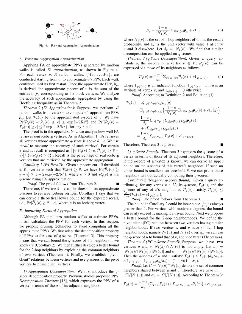
Fig. 4. Forward Aggregation Approximation

A. Forward Aggregation ApproximationApplying FA on approximate PPVs generated by random

walks is called FA approximation, as shown in Figure 4.For each vertex v, R random walks, {W1, . . . ,WR}, areconducted starting from v, to approximate v’s PPV. Each walkcontinues until its first restart. Once the approximate PPV, pv,is derived, the approximate q-score of v is the sum of theentries in pv corresponding to the black vertices. We analyzethe accuracy of such approximate aggregation by using theHoeffding Inequality as in Theorem 2.

Theorem 2 (FA Approximation): Suppose we perform Rrandom walks from vertex v to compute v’s approximate PPV,pv. Let Pq(v) be the approximated q-score of v. We havePr[Pq(v) " Pq(v) # "] $ exp{"2R"2} and Pr[|Pq(v) "Pq(v)| # "] $ 2 exp{"2R"2}, for any " > 0.

The proof is in the appendix. Now we analyze how well FAretrieves real iceberg vertices. As in Algorithm 1, FA retrievesall vertices whose approximate q-score is above !" ". We userecall to measure the accuracy of such retrieval. For certain! and ", recall is computed as

!!{v|Pq(v) # !, Pq(v) # ! ""}!!/!!{v|Pq(v) # !}

!!. Recall is the percentage of real icebergvertices that are retrieved by the approximate aggregation.

Corollary 1 (FA Recall): Given a q-score cut-off threshold!, for vertex v such that Pq(v) # !, we have Pr[Pq(v) #! " "] # 1 " 2 exp{"2R"2}, where " > 0 and Pq(v) is v’sq-score using FA approximation.

Proof: The proof follows from Theorem 2.Therefore, if we use !" " as the threshold on approximate

q-scores to retrieve iceberg vertices, Corollary 1 says that wecan derive a theoretical lower bound for the expected recall,i.e., Pr[Pq(v) # ! " "], where v is an iceberg vertex.

B. Improving Forward AggregationAlthough FA simulates random walks to estimate PPVs,

it still calculates the PPV for each vertex. In this section,we propose pruning techniques to avoid computing all theapproximate PPVs. We first adapt the decomposition propertyof PPVs to the case of q-scores (Theorem 3). This propertymeans that we can bound the q-scores of v’s neighbors if weknow v’s (Corollary 2). We then further develop a better boundfor the 2-hop neighbors by exploiting the common neighborsof two vertices (Theorem 4). Finally, we establish “pivot-client” relations between vertices and use q-scores of the pivotvertices to prune client vertices.

1) Aggregation Decomposition: We first introduce the q-score decomposition property. Previous studies proposed PPVDecomposition Theorem [18], which expresses the PPV of avertex in terms of those of its adjacent neighbors.

pv =1" c

|N1(v)|!x!N1(v)px + c1v, (3)

where N1(v) is the set of 1-hop neighbors of v, c is the restartprobability, and 1v is the unit vector with value 1 at entryv and 0 elsewhere. Let dv = |N1(v)|. We find that similardecomposition can be applied on q-scores.

Theorem 3 (q-Score Decomposition): Given a query at-tribute q, the q-score of a vertex v % V , Pq(v), can beexpressed via those of its neighbors as follows,

Pq(v) =1" c

dv!x!N1(v)Pq(x) + c1q!L(v), (4)

where 1q!L(v) is an indicator function: 1q!L(v) = 1 if q is anattribute of vertex v, and 1q!L(v) = 0 otherwise.

Proof: According to Definition 2 and Equation (3):

Pq(v) = !y|y!V,q!L(y)pv(y)

=!y|y!V,q!L(y)

" 1" c

|N1(v)|!x!N1(v)px(y) + c1v(y)

#

=1" c

dv!x!N1(v)!y|y!V,q!L(y)px(y)

+ c!y|y!V,q!L(y)1v(y)

=1" c

dv!x!N1(v)Pq(x) + c1q!L(v).

Therefore, Theorem 3 is proven.

2) q-Score Bounds: Theorem 3 expresses the q-score of avertex in terms of those of its adjacent neighbors. Therefore,if the q-score of a vertex is known, we can derive an upperbound on the q-scores of this vertex’s neighbors. If such anupper bound is smaller than threshold !, we can prune thoseneighbors without actually computing their q-scores.

Corollary 2 (Neighbor q-Score Bound): Given a query at-tribute q, for any vertex v % V , its q-score, Pq(v), and theq-score of any of v’s neighbor x, Pq(x), satisfy Pq(x) $dv1"c(Pq(v)" c1q!L(v)).

Proof: The proof follows from Theorem 3.The bound in Corollary 2 could be loose since dv

1"c is alwaysgreater than 1. For vertices with moderate degrees, the boundcan easily exceed 1, making it a trivial bound. Next we proposea better bound for the 2-hop neighborhoods. We define thepivot-client (PC) relation between two vertices having similarneighborhoods. If two vertices u and v have similar 1-hopneighborhoods, namely N1(u) and N1(v) overlap, we can usethe q-score of u to bound that of v, and vice versa (Theorem 4).

Theorem 4 (PC q-Score Bound): Suppose we have twovertices u and v. N1(u) & N1(v) is not empty. Let #u =|N1(u)&N1(v)|/|N1(u)| and #v = |N1(u)&N1(v)|/|N1(v)|.Then the q-scores of u and v satisfy: Pq(v) $ Pq(u)du/dv +c(1q!L(v) " 1q!L(u)du/dv) + (1 " c)(1" #v).

Proof: Let C = N1(u)&N1(v) denote the set of commonneighbors shared between u and v. Therefore, we have #u =|C|/|N1(u)| and #v = |C|/|N1(v)|. According to Theorem 3:

Pq(u) =1" c

du

$!x!CPq(x)+!x!N1(u)\CPq(x)

%+c1q!L(u),

v

u

dc

b

e

ga

Fig. 5. Pivot-Client Relation

Likewise, we have

Pq(v) =1" c

dv

$!x!CPq(x)+!x!N1(v)\CPq(x)

%+ c1q!L(v).

Combining the above two equations, we have:

Pq(v) =1" c

dv

$ du1" c

(Pq(u)" c1q!L(u))

" !x!N1(u)\CPq(x) + !x!N1(v)\CPq(x)%+ c1q!L(v)

=dudv

Pq(u) + c$1q!L(v) "

dudv

1q!L(u)

%

+1" c

dv

$!x!N1(v)\CPq(x)" !x!N1(u)\CPq(x)

%

$dudv

Pq(u) + c$1q!L(v) "

dudv

1q!L(u)

%

+1" c

dv!x!N1(v)\CPq(x). (5)

Since all entries of a PPV add up to 1, the aggregate valuefor any vertex v, Pq(v) $ 1. Therefore, we have:

1" c

dv!x!N1(v)\CPq(x) $

1" c

dv(|N1(v)|" |C|)

=(1" c)(1" #v). (6)

Applying Equation (6) to Equation (5), we have: Pq(v) $dudvPq(u) + c(1q!L(v) " du

dv1q!L(u)) + (1" c)(1 " #v).

If we choose u as the pivot and v as one of its clients, wecan use u’s q-score to bound v’s. If a pivot has a low q-score,likely some of its clients can be quickly pruned. Theorem 4shows that larger #v and #u lead to better bounds. Pivot-clientrelations are established as follows: for vertices u and v, ifthe common 1-hop neighbors take at least # fraction of eachvertex’s neighborhood, i.e., #u # # and #v # #, we designateeither of them as the pivot and the other as the client. Clearly,u and v are within 2-hop of each other. Theorem 4 bounds theq-scores for some of a pivot’s 2-hop neighbors. Figure 5 showsthat vertices u and v share four 1-hop neighbors in common:{a, b, c, d}. If # = 0.5, either of them can be the pivot of theother. Algorithm 2 shows how to find pivots and their clients.

3) Approximate q-Score Bounding and Pruning: The pro-posed q-score bounds express the relation between the real q-scores of vertices. However, computing real q-scores is costlyfor large graphs. Since random walks are used in gIceberg toapproximate PPVs and approximate q-scores are subsequentlycomputed, will those bounds still be effective for pruning? Inthis section, we analyze the effectiveness of using approximateq-scores to derive approximate q-score bounds. Our findings

Algorithm 2: Pivot Vertex SelectionInput: G, neighborhood similarity threshold #Output: Pivot vertices VP and their clients1 for Each unchecked v in V do2 Grow v’s 2-hop neighborhood N2(v) using BFS;3 For each unchecked u in N2(v), check if N1(u) and

N1(v) satisfy similarity threshold #; if so, insert u intov’s client set, insert v to VP and mark both v and u aschecked;

4 Return all pivot vertices VP and their clients;

are: given a q-score cut-off threshold !, if approximate q-scores are used to derive approximate q-score bounds as inCorollary 2 and Theorem 4, with some adjustment to !, thebounds can still be leveraged to prune vertices with a certainaccuracy. Specifically, those vertices pruned by those boundsare very likely to be real non-iceberg vertices. The details arein Theorems 5 and 6 and the proofs are in the appendix.

Theorem 5 (Approximate Neighbor Bound): Let x be anadjacent vertex of vertex v. For a given pruning cut-off thresh-old !, let !1 = !"dv"/(1"c)+". If dv

1"c (Pq(v)"c1q!L(v)) <

!1" ", where Pq(v) is the approximate q-score of v using FAapproximation with R random walks, then x can be prunedand we have Pr[Pq(x) < !] # 1" 2 exp{"2R"2}.

Theorem 6 (Approximate PC Bound): Suppose we havevertices u and v and N1(u) &N1(v) is not empty. Let #u =|N1(u)&N1(v)|/|N1(u)| and #v = |N1(u)&N1(v)|/|N1(v)|.For a given pruning cut-off threshold !, let !2 = !"du"/dv+".If Pq(u)du/dv+c(1q!L(v)"1q!L(u)du/dv)+(1"c)(1"#v) <!2" ", where Pq(u) is the approximate q-score of u using FAapproximation with R random walks, then v can be prunedand we have Pr[Pq(v) < !] # 1" 2 exp{"2R"2}.

To summarize, this section shows: (1) Two types of q-scorebounds can be used to prune non-iceberg verticess. (2) Whenrandom walks are used to approximate q-scores, the boundsbecome approximate too. However, with certain adjustment tothe thresholds and pruning rules, the likelihood for a prunedvertex to be a real non-iceberg vertex can be bounded. We willshow later in our experiments that PFA yields good recall inpractice. Algorithm 3 shows the workflow of PFA.

Algorithm 3: Pivot Vertex-Based Forward AggregationInput: G, query q, threshold !, neighborhood similarity

threshold #, approximation error "Output: Graph iceberg vertices1 Index all the pivot vertices VP using # as in Alg. 2;2 for Each v in VP do3 Use random walks to get v’s approximate PPV, pv;4 Get v’s approximate q-score using pv;5 Use approximate q-score bounds to prune vertices using

adjusted thresholds based on !;6 for Each v that is not pruned do7 Use random walks to get v’s approximate PPV, pv;8 Get v’s approximate q-score using pv;9 Return vertices with approximate q-score above ! ! ";

v

y

x

. . .

. . .

z

.. .

.... . .

.. .

W1

W 2

WRW 1

W 2

W2

W1W R WR

. . .

Fig. 6. Backward Aggregation Approximation

V. BACKWARD AGGREGATION

In this section, we introduce a different aggregation schemecalled backward aggregation (BA). Instead of aggregatingPageRank in a forward manner (adding up the entries ofblack vertices in a PPV), BA starts from black vertices, andpropagates values in their PPVs to other vertices in a backwardmanner. Specifically, based on the reversibility of randomwalks, the symmetric property of degree-normalized PPV [19]states that: in an undirected graph G, for any two vertices uand v, the PPVs of u and v satisfy:

pu(v) =dvdu

pv(u), (7)

where du and dv are the degrees of u and v, respectively.If we know v’s PageRank with respect to u, pu(v), we canquickly compute the value for its reverse, pv(u), withoutactually computing v’s PPV. For a given query attribute q,the PageRank values of black vertices in any vertex v’s PPVare the key to computing v’s q-score. In Figure 3(b), BA startsfrom black vertices, computes their PPVs, and propagates theircontributions to the other vertices’ q-scores backward (blackarrow) according to Equation (7). BA provides a possibilityto quickly compute q-scores for the entire vertex set, bystarting from only those black vertices. Given that blackvertices usually occupy a small portion of V , BA reduces theaggregation time significantly.

A. Backward Aggregation Approximation

Applying BA on approximate PPVs generated by randomwalks is called BA approximation. In Figure 6, for eachblack vertex x we perform R random walks, {W1, . . . ,WR},from x to approximate x’s PPV. Each walk continues untilits first restart. Once such process is done on all the blackvertices, for any vertex v in G, v’s approximate q-score isthe sum of the reverse PageRank scores of the vth entriesin the approximate PPVs of the black vertices, computedaccording to Equation (7). We now analyze the accuracy ofsuch approximate aggregation.

Theorem 7 (BA Approximation): Let Vq ! V be the set ofblack vertices. Suppose we perform R random walks fromeach black vertex, x, to approximate its PPV, px. For anyvertex v % V , let Pq(v) = !x!Vq

dxdv

px(v) be the approximateq-score of v using BA. We have Pr[Pq(v) " Pq(v) # "] $exp{"2Rd2v"

2/!x!Vqd2x} and Pr[|Pq(v) " Pq(v)]| # "] $

2 exp{"2Rd2v"2/!x!Vqd

2x}, where " > 0.

The proof is in the appendix. Now we analyze how wellBA retrieves iceberg vertices. As in Algorithm 4, BA retrieves

Algorithm 4: Backward AggregationInput: G, query q, threshold !, approximation error "Output: Graph iceberg vertices1 for Each black vertex x do2 Use random walks to get x’s approximate PPV, px;3 for Each entry px(v) do4 Compute the reverse entry pv(x) =

dxdv

px(v);

5 Add pv(x) to v’s q-score: Pq(v);6 Return vertices with approximate q-score above ! ! ";

all the vertices whose approximate q-score is above ! " "as iceberg vertices. Again we use recall as the measure,which evaluates the percentage of real iceberg vertices thatare captured by the BA approximation.

Corollary 3 (BA Recall): Given a q-score cut-off threshold!, for vertex v such that Pq(v) # !, we have Pr[Pq(v) #! " "] # 1 " 2 exp{"2Rd2v"

2/!x!Vqd2x}, where " > 0 and

Pq(v) is v’s q-score using BA approximation.Proof: The proof follows from Theorem 7.

Therefore the likelihood for a real iceberg vertex v to beretrieved by BA can be bounded. This bound is not as tightas the one for FA. We later show in our experiments that BAachieves good recall in practice, given a reasonable number ofrandom walks. Algorithm 4 describes the BA workflow.

VI. CLUSTERING PROPERTY OF ICEBERG VERTICES

Graph iceberg vertices can further be used to discover graphiceberg regions. We achieve this by methods ranging fromgraph clustering to simple connected component finding. Inthis section, we describe some interesting properties of howiceberg vertices are distributed in the graph. We discoveredthat iceberg vertices naturally form connected componentssurrounding the black vertices in the graph.

A. Active BoundaryDefine a region R = {VR, ER} to be a connected subgraph

of G, and the boundary of R, N(R), to be the set of verticessuch that N(R)&VR = ' and each vertex in N(R) is directlyconnected to at least one vertex in VR. In Figure 7(a), the darkarea surrounding region R forms R’s boundary. Theorem 3shows that the q-score of a non-black vertex is exactly (1" c)times the average q-score of all its neighbors.

Theorem 8 (Boundary): Given a region R in G which doesnot contain any black vertex, if the q-scores of all vertices inN(R) are below the q-score threshold !, then no vertex in VR

has q-score above !.Proof: Equation (4) shows that the q-score of a non-black

vertex is lower than the maximum q-score of its neighbors.Suppose there is a vertex v0 % VR such that Pq(v0) > !. SinceR does not contain black vertices, v0 is non-black, thus at leastone of v0’s neighbors has q-score higher than Pq(v0). Let itbe v1. The same argument holds for v1. A path is thereforeformed with a strictly increasing sequence of q-scores, and allthe q-scores in this sequence are > !. Since |VR| is finite,eventually the path goes through R’s boundary, N(R). Since

Active Bo undary

. . .

. . .

. . .. . .R

Gr aph G(a) Boundary (b) A ctive Boundary

Fig. 7. Boundary and Active Boundary

all vertices in N(R) have a q-score below !, a contradictionis reached. Therefore no such vertex v0 exists and all verticesin VR have q-scores below !.

Corollary 4 (Active Path): If vertex v is an iceberg vertex,there exists a path, called an “active path”, from v to a blackvertex, that all vertices on that path are iceberg vertices.

Proof: Assume there is an iceberg vertex v0 (non-black)that can not be linked to a black vertex via such a path. Againwe can follow a path starting from v0 to one of its neighbors,v1, an iceberg vertex, then to another such neighbor of v1,and so on. Such a path contains only iceberg vertices. A setof such paths form a region surrounding v0, containing onlyiceberg vertices. The boundary of this region only containsvertices with q-scores below !. The assumption dictates thereis no black vertex in this region. This contradicts Theorem 8.So no such vertex v0 exists.

Corollary 5 (Active Region & Active Boundary): Given aquery attribute q and q-score threshold !, all iceberg vertices inG concentrate surrounding black vertices. Each black vertexis surrounded by a region containing only iceberg vertices,which is called “active region”. The boundary of such a regionis called “active boundary”. The q-scores of the vertices in theactive boundary are all below !.

Proof: The proof follows from Corollary 4.Corollary 5 suggests that in order to retrieve all iceberg

vertices, we only need to start from black vertices and growtheir active regions. The key to grow an active region of ablack vertex is to find the active boundary of this region. It ispossible that several active regions merge into one if the blackvertices are close to each other. Figure 7(b) shows examplesof active regions and boundaries. Black vertices contain thequery attribute and gray vertices are iceberg vertices. Eachblack vertex is embedded in an active region containing onlyiceberg vertices, which is encompassed by a solid black line.All the white vertices between the solid black line and the reddashed line form the active boundaries of those regions. Allvertices with grid pattern which are not in any active regionhave a q-score below the threshold.

Therefore, we have discovered this interesting “clustering”property of iceberg vertices. All iceberg vertices tend to clusteraround the black vertices in the graph, which automaticallyform several interesting iceberg regions in the graph. Thesize of an iceberg region can be controlled by varying theq-score threshold.

VII. EXPERIMENTS

gIceberg is evaluated using both real-world and syntheticdata. We first conduct motivational case studies on the DBLPnetwork to show that gIceberg is able to find interestingauthor groups. The remaining experiments focus on: (i) ag-gregation accuracy; (ii) forward aggregation (FA) and back-ward aggregation (BA) comparison; (iii) impact of attributedistributions; and (iv) scalability. We observe that: (1) Randomwalk approximation achieves good accuracy. (2) FA is slightlybetter than BA in recall and precision, while BA is generallymuch faster. (3) Pivot vertex selection and q-score boundingeffectively reduce runtime. (4) gIceberg is robust to variousattribute distributions, and BA is efficient even for denseattribute distribution; (5) BA scales well on large graphs. Allthe experiments are conducted on a machine that has a 2.5GHzIntel Xeon processor, 32G RAM, and runs 64-bit Fedora 8with LEDA 6.0 [20]. Figures are best viewed in color.

A. Data SetsCustomer Network (Customer). This is a proprietary data

set provided by an e-commerce corporation offering onlineauction and shopping services. The vertices are customers andthe edges are their social interactions. The attributes of a vertexare the products that the customer has purchased. This graphhas 794,001 vertices, 1,370,284 edges, and 85 product names.

DBLP Network (DBLP). This is built from the DBLP1

repository. Each vertex is an author and each edge represents aco-authorship. The keywords in paper titles are used as vertexattributes. We use a subset of DBLP containing 130 importantkeywords extracted by Khan et al. [21]. This graph contains387,547 vertices and 1,443,873 edges.

R-MAT Synthetic Graphs (R-MAT). A set of syntheticgraphs with power-law degree distributions and small-worldcharacteristics are generated by the GTgraph toolkit2 usingthe Recursive Matrix (R-MAT) graph model [22]. The vertexnumber spans across 500K , 2M , 4M , 6M , 8M , 10M . Theedge number spans across 3M , 8M , 16M , 24M , 32M , 40M .

TABLE IQUERY ATTRIBUTE EXAMPLES

Data Sets Query Attribute Examples

Customer “Estee Lauder Eye Cream”, “Ray-Ban Sunglasses”“Gucci Glasses”, “A&F Women Sweatshirts”

DBLP“Database”, “Mining”, “Computation”“Graph”, “Classification”, “Geometry”

50 queries are used for each graph. Table I shows somequery examples for Customer and DBLP. The attribute gen-erator for R-MAT will be introduced in Section VII-E. Theq-score threshold is ! = 0.5, if not otherwise specified.

B. Case StudyTo show that gIceberg finds interesting vertices in a real

graph, we conduct a case study on DBLP: (1) given a user

1www.informatik.uni-trier.de/!ley/db/2http://www.cse.psu.edu/!madduri/software/GTgraph/

I. Manolescu ( 43)T. Milo (30) A. Boni fati ( 26)

D. Florescu (22)

S. Ab iteboul ( 55)

V. Vianu (20)

A. Pug liese ( 18)D. Suci u ( 29)

M. J. Ca rey (16)

. . .

. . .

. . .

Threshold = 0.33Threshold = 0.3

S. Par abos chi (15) L. T anca (17)

“XML”

(a) Keyword: “XML”

S. Madden (8)

U. Çe tintemel ( 20) S. B. Z donik (20)

Y. Xing (9)

N. Tat bul (14)

M. Ch erniack (9)

M. Bala zinska (9) M. St onebraker ( 11)

. . .. . .

Threshold = 0.2 7Threshold = 0.24

“S tream”

J. H. Hwang (13)

(b) Keyword: “Stream”

Fig. 8. Case Studies on DBLP

0.5

0.6

0.7

0.8

0.9

1

10 100 500 2000

Acc

urac

y

Number of Random Walks

FABA

(a) Customer Subgraph

0.5

0.6

0.7

0.8

0.9

1

10 100 500 2000

Acc

urac

y

Number of Random Walks

FABA

(b) DBLP 2010

0.5

0.6

0.7

0.8

0.9

1

10 100 500 2000

Acc

urac

y

Number of Random Walks

FABA

(c) R-MAT 3K

Fig. 9. Random Walk-Based Aggregation Accuracy

specified research topic and an iceberg threshold, we findthe iceberg vertices and remove the rest; (2) these verticesform several connected components in the remaining graph.The iceberg vertices imply that many of their neighbors havepublished in the user specified topic. Therefore, the compo-nents shall represent collaboration groups in that area. We willdemonstrate that gIceberg can indeed discover interesting andimportant author groups.

Figure 8 shows the top author groups found by gIcebergfor two query keywords: “XML” and “Stream”. The numbernext to each author’s name is the number of his/her publi-cations in that keyword field. All the vertices who have 7+papers containing the query keyword are retained. There is anedge between two authors if they have collaborated at least7 times. In gIceberg, we set the threshold at a small valueand increase it until the author groups become small enough.Take “Stream” for example: the author group size decreasesfrom 9 to 6, as threshold increases from 0.24 to 0.27. For0.27, the current author group contains 6 authors (in blue).It seems the author groups that gIceberg discovers are ofhigh-quality. They are specialized and well-known in the fieldof “XML” and “Stream”. In addition, by varying the q-scorethreshold, users can easily zoom in and zoom out the authorgroups and exploit the hierarchical structure with views ofmultiple granularities. Such zoom in/out effect is not availableif we simply use the number of papers as a filter, which willgenerate many small disconnected components. For example,in Figure 8(b), likely only U. Cetintemel and S. Zdonik willbe ranked high, and the others will not show up at all.

C. Aggregation AccuracyWe now evaluate the accuracy of random walk approxi-

mation. We compare random walk-based FA and BA, with

the power method-based aggregation, which aggregates overPPVs generated by the power method. We conduct the poweriteration until the maximum difference between any entries oftwo successive vectors is within 10"6. Since the power methodis time consuming, this test is done on three small graphs:Customer Subgraph is a subgraph of Customer with 5,000vertices and 14,735 edges; DBLP 2010 is the DBLP networkthat spans from January 2010 to March 2010, with 12,506vertices and 19,935 edges; RMAT 3K is a synthetic graphgenerated by the GTgraph toolkit, with 3,697 vertices and7,965 edges. All three small graphs are treated as independentgraphs. Accuracy is defined as the number of vertices, whoseFA (or BA) approximate q-score falls in between ["",+"] ofits q-score computed by the power method, divided by the totalnumber of vertices. We then compute the average accuracyover all the queries. The mean accuracy with standard errorbars is shown in Figure 9 (" = 0.03). We vary the number ofrandom walks performed on each vertex. Both FA and BA areshown to empirically produce good accuracy with high meanand low standard error. Since the power method is very slow,hereinafter we apply FA with 2K random walks per vertex onlarger graphs to provide “ground truth” q-scores.

D. Forward vs. Backward AggregationWe now compare forward and backward aggregation using

recall, precision and runtime.1) Recall and Runtime: Recall is defined as the number of

iceberg vertices retrieved by gIceberg, divided by the totalnumber of iceberg vertices, i.e.,

!!{v|Pq(v) # !, Pq(v) #!""}

!!/!!{v|Pq(v) # !}

!!, where Pq(v) and Pq(v) are true andapproximate q-scores, respectively. The effectiveness of pivotvertex, approximate q-score bounding and pruning in pivotvertex-based FA (PFA) is also evaluated. In PFA, 150 random

0.5

0.6

0.7

0.8

0.9

1

0.01 0.02 0.03 0.04 0.05

Rec

all

Error Tolerance,

FAPFABA

(a) Customer, R = 500

0.5

0.6

0.7

0.8

0.9

1

10 100 500 2000

Rec

all

Number of Random Walks

FAPFABA

(b) Customer, " = 0.03

138

2050

1203008002K5K

15K

10 100 500 2000

Avg

. Run

time

in S

econ

ds

Number of Random Walks

FA PFA BA

(c) Customer, Runtime

0.5

0.6

0.7

0.8

0.9

1

0.01 0.02 0.03 0.04 0.05

Rec

all

Error Tolerance,

FAPFABA

(d) DBLP, R = 500

0.5

0.6

0.7

0.8

0.9

1

10 100 500 2000

Rec

all

Number of Random Walks

FAPFABA

(e) DBLP, " = 0.03

138

2050

1203008002K6K

10 100 500 2000

Avg

. Run

time

in S

econ

ds

Number of Random Walks

FA PFA BA

(f) DBLP, Runtime

Fig. 10. Forward Aggregation vs. Backward Aggregation: Recall and Runtime Comparison

0

0.2

0.4

0.6

0.8

1

0.01 0.02 0.03 0.04 0.05

Prec

isio

n

Error Tolerance,

FAPFABA

(a) Customer, R = 2000

0

0.2

0.4

0.6

0.8

1

10 100 500 2000

Prec

isio

n

Number of Random Walks

FAPFABA

(b) Customer, " = 0.01

0

0.2

0.4

0.6

0.8

1

0.01 0.02 0.03 0.04 0.05

Prec

isio

n

Error Tolerance,

FAPFABA

(c) DBLP, R = 2000

0

0.2

0.4

0.6

0.8

1

10 100 500 2000

Prec

isio

n

Number of Random Walks

FAPFABA

(d) DBLP, " = 0.01

Fig. 11. Forward Aggregation vs. Backward Aggregation: Precision Comparison

walks are applied on each pivot vertex, while R randomwalks are applied on the rest. Figure 10 shows the recalland runtime for Customer and DBLP. We plot the averagerecall over all queries with error bars on each point. Thefirst column shows how recall changes with ", for R = 500;the second column shows how recall changes with R, for" = 0.03. We can observe that: (1) Both FA and PFA yieldhigh recall and BA yields satisfying recall when R is # 500.The approximation captures most of the real iceberg vertices.(2) The standard error across various queries is small for allthe methods, showing the performance is consistent and robustto various queries. (3) Recall increases with " and R, which isas expected. (4) It is reasonable that PFA produces better recallthan FA when R $ 150, even though PFA uses approximate q-score bounding. This is because for all R values, 150 randomwalks are always applied on pivot vertices in PFA. Thus whenR $ 150, more random walks are used in PFA than in FA.

Runtime comparison in Figure 10 shows that BA signifi-cantly reduces the runtime. When R is large, PFA reduces theruntime of FA via pivot vertex and q-score bounding. Since thepivot vertices use 150 random walks, it is expected for PFAto cost more time than FA when R is small. When R = 100,

TABLE IIPIVOT VERTEX INDEXING COST

Data Sets Customer DBLP RMAT 500KTime (Hours) 0.176 0.162 1.230

Index/Graph Size (MB) 8.48/46.53 4.75/91.68 9.24/53.99

PFA is still faster than FA, due to effective pruning. Table IIshows that it takes a reasonable amount of offline computationto select pivot vertices. To sum up, BA still yields good recallwhile reducing the runtime. FA is preferred over BA whenhigher recall is desired.

2) Precision: Precision is defined as the number of icebergvertices retrieved by gIceberg, divided by the total numberof retrieved vertices, i.e.,

!!{v|Pq(v) # !, Pq(v) # ! ""}!!/!!{v|Pq(v) # ! " "}

!!. Figure 11 shows the curves ofthe average precision over all queries with error bars forCustomer and DBLP. We can see that: (1) FA and PFA yieldbetter precision than BA. When R = 2000, all the methodsyield decent precision. (2) The standard error is small for allthe methods, showing the performance is consistent acrossqueries. (3) Precision decreases with " and increases with R

00.10.20.30.40.50.60.70.80.9

1

0.1% 1% 10%

Rec

all

Percentage of Black Vertices

FA PFA BA

(a) Recall vs. Percentage

138

2050

120300800

0.1% 1% 10%

Avg

. Run

time

in S

econ

ds

Percentage of Black Vertices

FA (R=300)PFA (R=300)BA (R=1200)

(b) Runtime vs. Percentage

00.10.20.30.40.50.60.70.80.9

1

10 20 100

Rec

all

# of Black Vertices Concentrated Locally,

FA PFA BA

(c) Recall vs. Skewness

138

2050

120250600

10 20 100

Avg

. Run

time

in S

econ

ds

# of Black Vertices Concentrated Locally,

FA (R=300)PFA (R=300)BA (R=1200)

(d) Runtime vs. Skewness

Fig. 12. Attribute Distribution Test

as expected. (4) As previously analyzed, it is reasonable forPFA to produce better precision than FA when R $ 150.

We can see that BA is much faster than FA and BA yieldsgood recall when R # 500. However, the precision of BAis not satisfactory unless R # 2000. FA overall yields betterprecision than BA. Therefore a fast alternative to achieve bothgood recall and precision would be: (1) apply BA to retrievemost real iceberg vertices with good recall; and then (2) applyFA on those retrieved vertices to prune out the “false positives”to further achieve good precision.

E. Attribute Distribution

We now test the impact of attribute distribution on theaggregation performance. To customize the attribute distri-bution, a synthetic R-MAT graph with 514,632 vertices and2,998,960 edges is used (R-MAT 500K). Two tests are done:(1) We customize the percentage of the black vertices, which iscomputed as |Vq|/|V |. Given a query attribute q, we randomlydistribute it into the graph. The set of black vertices is Vq . (2)We customize the skewness of the black vertex distribution.The attribute q can be randomly dispersed without any specificpatterns, or concentrated in certain regions. To instantiate thisidea, we randomly select a set of root vertices, and randomlyassign q to a certain number, $, of vertices within each root’sclose neighborhood. Let |Vr| be the total number of roots. Wehave $ ( |Vr| = |Vq|. If |Vq| is fixed, by tuning $ and |Vr|, wecan control the skewness of the attribute distribution. A higher$ indicates a higher skewness. We set " = 0.05, R = 300 forFA and PFA, and R = 1200 for BA.

For percentage test, 50 queries are randomly generatedfor each percentage. Figure 12(a) plots the mean recall withstandard error. The percentage varies from 0.1% to 10%. Allthree methods yield good recall with small standard errors.The recall slightly decreases when the percentage increases.Figure 12(b) shows that the runtime of BA increases with|Vq|/|V |, which is as expected. BA is much faster, even whenits random walk number is four times that of FA and PFA.

For skewness test, 50 queries are randomly generated foreach $. Figure 12(c) plots the mean recall with standard error.The number of black vertices concentrated locally surroundingeach root vertex, $, changes from 10 to 100. The black vertexnumber is |Vq| = 50K . All the methods yield good recall withsmall standard errors. PFA yields slightly worse recall, dueto approximate q-score bounding and pruning. Figure 12(d)

shows the BA runtime is almost constant because |Vq| isconstant and BA is significantly faster.

These figures show that FA/BA are not sensitive to theskewness in terms of recall and runtime. BA is sensitive tothe percentage of black vertices in terms of runtime, but notsensitive in terms of recall.

F. Scalability TestAs shown in previous experiments, BA is much more effi-

cient than FA and PFA. We further demonstrate how scalableBA is on large graphs. A set of R-MAT synthetic graphswith |V | ={2M , 4M , 6M , 8M , 10M} and |E| ={8M ,16M , 24M , 32M , 40M} are generated. The percentage ofblack vertices is 0.5% for all. The skewness of the attributedistribution, $, changes from 10 to 100. We set " = 0.05 andR = 250 for BA. Figure 13(a) plots the mean recall of BA withstandard errors across all the queries. BA yields good recallon all the graphs and the recall is not sensitive to attributedistribution skewness. Figure 13(b) shows that the runtime ofBA is approximately linear to the graph size. In conclusion,BA exhibits good scalability over large graphs. FA and PFA donot scale as well as BA. It takes them a few hours to return onlarge graphs. Therefore, we consider BA as a scalable solutionfor large graphs with decent recall. If higher recall is desired,users can choose FA instead of BA.

0.5

0.6

0.7

0.8

0.9

1

2M 4M 6M 8M 10M

Rec

all

Graph Size, |V|

=10=20

=100

(a) Recall

02468

1012

2M 4M 6M 8M 10M

Run

time

in M

inut

es

Graph Size, |V|

BA (R=250)

(b) Runtime

Fig. 13. BA Scalability Test

VIII. RELATED WORK

Graph iceberg analysis is related to the following areas.Iceberg cube and graph OLAP. In multidimensional

OLAP [23], an iceberg cube contains cells whose measuresatisfies a threshold [4], [23]. Existing iceberg cubing methodsinclude top-down methods, bottom-up methods, integrationmethods [23], [24], etc. Iceberg analysis on graphs has

been under-explored due to the absence of dimensionality ingraph data. The first work to place graphs in a rigid multi-dimensional and multi-level framework is [4]. The objectiveand results in [4] are substantially different from those in thispaper. With a distinct focus on iceberg analysis, we define theconcept of graph icebergs and propose scalable solutions.

Graph aggregation. Graph aggregation is to summarizeor aggregate networks to form a hierarchy. SNAP operationswere introduced in [2] to consistently merge nodes and edgeswith respect to a predefined hierarchy. When such hierarchyis unknown, graph summarization can be achieved via graphclustering [25]. A local neighborhood aggregation frameworkwas proposed in [5], which finds the top-k vertices with thehighest aggregation values over their neighbors. Our workextends [5] by incorporating local proximities to the targetattribute, into the aggregation.

Graph anomaly detection. Anomaly detection has beenstudied in graph-based data [3], [26], [27]. [26] proposed bothanomalous substructure detection and anomalous subgraphdetection. [3] discovered several new rules in density, weights,ranks and eigenvalues that govern local neighborhoods andused these rules for anomaly detection. gIceberg insteadfocuses on retrieving graph vertices interesting to a certainquery via aggregation. There is a distinct difference betweengraph anomaly and graph iceberg. However, the anomaly scoreof a vertex can be treated as its attribute value. Thus, graphanomaly detection can be used in gIceberg to find icebergswith many abnormal close neighbors.

Densest subgraph finding. In traditional densest subgraphstudies, the subgraph density is defined as the average vertexdegree of the subgraph [28], [29]. The densest k-subgraph(DkS) problem finds the densest subgraph of k vertices,which is NP-hard [30]. Most of these studies only considergraph connectivity. [6] introduces the novel problem of findingcohesive patterns. A cohesive pattern is a connected subgraphwhose density exceeds a given threshold and has homogeneousfeature values. What makes gIceberg different from [6] is thatthe iceberg regions discovered via clustering iceberg verticesinclude, but not limited to, dense regions. If an edge-sparseregion contains a high percentage of black vertices, it willlikely form an iceberg region as well, since the vertices withinwill have high q-scores.

Local clustering. Local clustering finds a cluster containinga given vertex without looking at the whole graph [12], [31]. Acore method called Nibble was proposed in [31]. By usingthe personalized PageRank [11] to define the nearness, [12]introduced an improved version, PageRank-Nibble. gIce-berg can be combined with standard graph clustering tech-niques to find iceberg regions. By aggregating over PPVs todefine the nearness between a vertex and an attribute, gIce-berg considers both vertex attributes and edge connectivities.

IX. CONCLUSIONS

This paper introduces a novel concept, graph iceberg, whichextends iceberg queries to vertex-attributed graphs and identi-fies interesting vertices that are close to an attribute using an

aggregate score. A scalable framework, gIceberg, is proposedwith two aggregation schemes: forward and backward aggrega-tion. Optimization techniques are designed to prune unpromis-ing vertices and reduce aggregation cost. Experiments on real-world and synthetic large graphs show the effectiveness andscalability of gIceberg. Future work includes finding icebergsincrementally on time-evolving graphs, and discovering othertypes of icebergs such as paths, trees, and subgraph patterns.

ACKNOWLEDGMENT

This research was sponsored in part by NSF IIS-0905084and by the Army Research Laboratory under cooperativeagreements W911NF-09-2-0053 and W911NF-11-2-0086. Theviews and conclusions contained herein are those of the au-thors and should not be interpreted as representing the officialpolicies, either expressed or implied, of the Army ResearchLaboratory or the U.S. Government. The U.S. Government isauthorized to reproduce and distribute reprints for Governmentpurposes notwithstanding any copyright notice herein.

REFERENCES

[1] X. Yan and J. Han, “gspan: Graph-based substructure pattern mining,”in ICDM, 2002, pp. 721–724.

[2] Y. Tian, R. A. Hankins, and J. M. Patel, “Efficient aggregation for graphsummarization,” in SIGMOD, 2008, pp. 567–580.

[3] L. Akoglu, M. McGlohon, and C. Faloutsos, “oddball: Spotting anoma-lies in weighted graphs,” in PAKDD, 2010, pp. 410–421.

[4] C. Chen, X. Yan, F. Zhu, J. Han, and P. S. Yu, “Graph OLAP: amulti-dimensional framework for graph data analysis,” Knowl. Inf. Syst.,vol. 21, no. 1, pp. 41–63, 2009.

[5] X. Yan, B. He, F. Zhu, and J. Han, “Top-k aggregation queries overlarge networks,” in ICDE, 2010, pp. 377–380.

[6] F. Moser, R. Colak, A. Rafiey, and M. Ester, “Mining cohesive patternsfrom graphs with feature vectors,” in SDM, 2009, pp. 593–604.

[7] A. Prakash, N. Valler, D. Andersen, M. Faloutsos, and C. Faloutsos,“Bgp-lens: patterns and anomalies in internet routing updates,” in KDD,2009, pp. 1315–1324.

[8] P. Bogdanov, M. Mongiov, and A. Singh, “Mining heavy subgraphs intime-evolving networks,” in ICDM, 2011, pp. 81–90.

[9] M. Fang, N. Shivakumar, H. Garcia-Molina, R. Motwani, and J. D.Ullman, “Computing iceberg queries efficiently,” in VLDB, 1998, pp.299–310.

[10] T. L. Fond and J. Neville, “Randomization tests for distinguishing socialinfluence and homophily effects,” in WWW, 2010, pp. 601–610.

[11] L. Page, S. Brin, R. Motwani, and T. Winograd, “The PageRank citationranking: Bringing order to the web,” Stanford InfoLab, Technical Report,1999.

[12] R. Andersen, F. R. K. Chung, and K. J. Lang, “Local partitioning fordirected graphs using PageRank,” Internet Mathematics, vol. 5, no. 1,pp. 3–22, 2008.

[13] M. Franceschet, “PageRank: Standing on the shoulders of giants,”Commun. ACM, vol. 54, no. 6, pp. 92–101, 2011.

[14] B. Bahmani, A. Chowdhury, and A. Goel, “Fast incremental andpersonalized PageRank,” PVLDB, vol. 4, no. 3, pp. 173–184, 2010.

[15] P. Berkhin, “Bookmark-coloring approach to personalized PageRankcomputing,” Internet Mathematics, vol. 3, no. 1, 2006.

[16] D. Fogaras, B. Racz, K. Csalogany, and T. Sarlos, “Towards scaling fullypersonalized PageRank: Algorithms, lower bounds, and experiments,”Internet Mathematics, vol. 2, no. 3, 2005.

[17] W. Hoeffding, “Probability inequalities for sums of bounded randomvariables,” J. Amer. Statistical Assoc., vol. 58, no. 301, pp. 13–30, 1963.

[18] G. Jeh and J. Widom, “Scaling personalized web search,” in WWW,2003, pp. 271–279.

[19] P. Sarkar and A. W. Moore, “Fast nearest-neighbor search in disk-resident graphs,” in KDD, 2010, pp. 513–522.

[20] K. Mehlhorn and S. Naher, LEDA: A Platform for Combinatorial andGeometric Computing. Cambridge University Press, 1999.

[21] A. Khan, X. Yan, and K.-L. Wu, “Towards proximity pattern mining inlarge graphs,” in SIGMOD, 2010, pp. 867–878.

[22] D. Chakrabarti, Y. Zhan, and C. Faloutsos, “R-MAT: A recursive modelfor graph mining,” in SDM, 2004.

[23] K. S. Beyer and R. Ramakrishnan, “Bottom-up computation of sparseand iceberg cubes,” in SIGMOD, 1999, pp. 359–370.

[24] D. Xin, J. Han, X. Li, and B. W. Wah, “Star-cubing: Computing icebergcubes by top-down and bottom-up integration,” in VLDB, 2003, pp. 476–487.

[25] A. Y. Wu, M. Garland, and J. Han, “Mining scale-free networks usinggeodesic clustering,” in KDD, 2004, pp. 719–724.

[26] C. C. Noble and D. J. Cook, “Graph-based anomaly detection,” in KDD,2003, pp. 631–636.

[27] J. Sun, H. Qu, D. Chakrabarti, and C. Faloutsos, “Neighborhoodformation and anomaly detection in bipartite graphs,” in ICDM, 2005,pp. 418–425.

[28] M. Charikar, “Greedy approximation algorithms for finding dense com-ponents in a graph,” in APPROX, 2000, pp. 84–95.

[29] S. Khuller and B. Saha, “On finding dense subgraphs,” in ICALP (1),2009, pp. 597–608.

[30] A. Bhaskara, M. Charikar, E. Chlamtac, U. Feige, and A. Vijayaragha-van, “Detecting high log-densities: An O(n1/4) approximation for dens-est k-subgraph,” in STOC, 2010, pp. 201–210.

[31] D. A. Spielman and S.-H. Teng, “A local clustering algorithm for mas-sive graphs and its application to nearly-linear time graph partitioning,”CoRR, vol. abs/0809.3232, 2008.

APPENDIX

Proof of Theorem 1:Proof: For each random walk Wi(i = {1, . . . , R}), let

Xi be a random variable such that

Xi =

&1, if random walk Wi ends at vertex x,0, otherwise.

Thus we have pv(x) = ( !iXi)/R. According to the findingsin [16], pv(x) = E[pv(x)]. From the definition of Xi, we havePr[Xi % [0, 1]] = 1, and Xi(i = {1, . . . , R}) are independentvariables, therefore according to Hoeffding Inequality, we canderive

Pr[!iXi

R" E[

!iXi

R] # "] $ exp{" 2(R")2

!i=Ri=1 (1 " 0)2

}

$ exp{"2R"2}.Therefore, we have Pr[pv(x) " pv(x) # "] $ exp{"2R"2}and Pr[|pv(x) " pv(x)| # "] $ 2 exp{"2R"2}.

Proof of Theorem 2:Proof: Recall that a vertex which contains attribute q

is called a black vertex. For each random walk Wi(i ={1, . . . , R}), let Yi be a random variable such that

Yi =

&1, if random walk Wi ends at a black vertex,0, otherwise.

Thus we have Pq(v) = ( !iYi)/R and Pq(v) = E[(!iYi)/R].According to the definition of Yi, Pr[Yi % [0, 1]] = 1, andYi(i = {1, . . . , R}) are independent variables. Therefore,according to Hoeffding Inequality, we can derive

Pr[!iYi

R" E[

!iYi

R] # "] $ exp{" 2(R")2

!i=Ri=1 (1" 0)2

}

$ exp{"2R"2}.

Similarly, we have Pr[|Pq(v)"Pq(v)| # "] $ 2 exp{"2R"2}.

Proof of Theorem 5:Proof: Since dv

1"c (Pq(v) " c1q!L(v)) < !1 " ", we havePq(v) <

(1"c)(!1"")dv

+ c1q!L(v). From Theorem 2, we knowPr[Pq(v) " " $ Pq(v) $ Pq(v) + "] # 1 " 2 exp{"2R"2}.Thus Pr[Pq(v) $ Pq(v) + " < (1"c)(!1"")

dv+ c1q!L(v) + "] #

1"2 exp{"2R"2}. Based on !1 = !"dv"/(1"c)+", we canderive Pr[ dv

1"c(Pq(v)" c1q!L(v)) < !] # 1" 2 exp{"2R"2}.So from Corollary 2, Pr[Pq(x) < !] # 1"2 exp{"2R"2}.

Proof of Theorem 6:Proof: Let B = c(1q!L(v)"1q!L(u)du/dv)+(1" c)(1"

#v). Since Pq(u)du/dv + c(1q!L(v) " 1q!L(u)du/dv) + (1"c)(1 " #v) < !2 " ", we have Pq(u) < dv(!2"""B)

du. From

Theorem 2, we know Pr[Pq(u) " " $ Pq(u) $ Pq(u) +"] # 1 " 2 exp{"2R"2}. Thus Pr[Pq(u) $ Pq(u) + " <dv(!2"""B)

du+ "] # 1 " 2 exp{"2R"2}. Based on !2 = ! "

du"/dv + ", we can derive Pr[Pq(u)du/dv + B < !] # 1 "2 exp{"2R"2}. So from Theorem 4, Pr[Pq(v) < !] # 1 "2 exp{"2R"2}.

Proof of Theorem 7:Proof: For any vertex v, for each random walk W x

i (i ={1, . . . , R}, x % Vq) starting from black vertex x, let Zx

i be arandom variable such that

Zxi =

&1, if random walk W x

i ends at a v,0, otherwise.

Thus we have px(v) = ( !iZxi )/R. px(v) = E[(!iZx

i )/R].By Equation (7), we have pv(x) = dx

dv(!iZx

i )/R and pv(x) =

E[dxdv(!iZx

i )/R]. We therefore can further derive

Pq(v) = !x!Vq pv(x) = !x!Vq

$dxdv

(!iZxi )/R

%

= !x!Vq!idxZx

i

dvR,

Pq(v) = E[!x!Vqpv(x)] = E[!x!Vq!idxZx

i

dvR].

Let Axi = dxZ

xi

dvR. Ax

i is a random variable such that Pr[Axi %

[0, dxdvR

]] = 1 and Axi (i = {1, . . . , R}, x % Vq) are inde-

pendent from each other. We have Pq(v) = !x!iAxi and

Pq(v) = E[!x!iAxi ]. According to Hoeffding Inequality,

Pr[Pq(v)" Pq(v) # "] = Pr[!x!iAxi " E[!x!iA

xi ] # "]

$ exp{" 2"2

!x!Vq!i=Ri=1

d2x

d2vR

2

} $ exp{" 2Rd2v"2

!x!Vqd2x}.

Similarly Pr[|Pq(v) " Pq(v)]| # "] $ 2 exp{" 2Rd2v"

2

!x!Vq d2x}.